


Abstract
Free-floating space manipulators are strongly coupled systems in which manipulator motion affects spacecraft base motion through momentum exchange, making simultaneous end-effector control and disturbance suppression challenging. This work investigates how an additional actuated prismatic degree of freedom influences whole-arm coordination in a 6R1P free-floating space manipulator. Compared with a fixed-length 6R configuration, the prismatic joint enlarges the feasible motion space and introduces an additional motion-allocation direction for full-pose tasks under generalized-Jacobian constraints. A proximal policy optimization (PPO)-based controller is developed for full-pose reaching with spacecraft-motion-aware objectives. Simulation results show that the 6R1P configuration improves reaching performance and reduces spacecraft reaction compared with the locked-prismatic 6R baseline. Trajectory-level dynamic reconstruction further reveals that the disturbance reduction is not caused by direct cancellation from the prismatic joint itself, but mainly by configuration-dependent redistribution of revolute-joint motions and enhanced mutual cancellation among their reaction contributions. These results demonstrate that telescopic redundancy provides a mechanism for coordinated motion allocation in free-floating manipulation, enabling learned policies to exploit additional degrees of freedom for improved task execution and reduced spacecraft disturbance.
1. Introduction
As the demand for on-orbit servicing, assembly, inspection and maintenance, refueling, active debris removal, and in-space manufacturing continues to increase, robotic manipulation is becoming an important enabling technology for future space infrastructure. Space manipulators can extend spacecraft service life, support the construction and maintenance of large orbital structures, and interact physically with both cooperative and noncooperative targets. In many of these tasks, the manipulator may operate in a free-floating mode, where thrusters or other active position- and attitude-control actuators are not used continuously to stabilize the spacecraft base during arm motion. This operating mode reduces propellant consumption and avoids plume effects on nearby targets. Its main difficulty, however, is the dynamic interaction between the manipulator and the spacecraft. Reaction forces and torques generated by joint motion cause translation and rotation of the base, while the resulting base motion alters the actual motion of the end effector. End-effector task execution and spacecraft disturbance are therefore coupled objectives in a free-floating system and cannot be treated independently [1,2,3,4,5,6].
The dynamic coupling of free-floating manipulators has been studied since the early development of space robotics. Umetani and Yoshida introduced the Generalized Jacobian Matrix (GJM), incorporating momentum conservation into the relationship between manipulator joint motion and end-effector motion [7]. Papadopoulos and Dubowsky subsequently examined the structure of control algorithms for free-floating manipulators [8]. Later theoretical and experimental studies established a broader framework covering kinematics, dynamics, nonholonomic constraints, momentum coupling, and on-orbit validation. These studies show that spacecraft motion results from momentum-constrained inertial coupling between the base and the manipulator. The effect of a given joint motion depends on the instantaneous arm configuration, link geometry, and mass distribution of the complete multibody system. The GJM provides a convenient description of end-effector motion while accounting for this base response. Consequently, a joint motion that produces a favorable response in one configuration may not do so in another, making free-floating coupling strongly configuration-dependent [7,8,9,10,11,12,13,14,15,16,17,18,19].
A variety of methods have been developed to reduce the spacecraft reaction caused by manipulator motion. Reactionless-motion and reaction-null-space methods exploit redundant degrees of freedom or particular coupling structures to construct joint motions with reduced base reaction [10,11]. Related work has extended this idea to point-to-point planning, constrained optimization, direct trajectory optimization, model predictive control, and task-priority control, allowing end-effector tracking, base disturbance, joint limits, collision avoidance, singularity avoidance, and computational cost to be considered simultaneously [13,20,21,22]. These model-based approaches have clear physical interpretations and, in some cases, provide strong theoretical guarantees. Their implementation, however, often requires explicit kinematic or dynamic models together with repeated evaluation of configuration-dependent matrices, matrix inversion, or online numerical optimization. Moreover, redundancy alone does not guarantee lower spacecraft disturbance. Whether an additional degree of freedom is useful depends on the rank and structure of both the task mapping and the dynamic coupling [10]. Its value therefore lies in the additional possibilities it provides for coordinating motion and redistributing momentum.
This point is particularly relevant to space manipulators equipped with controllable prismatic or telescopic joints. Unlike conventional serial manipulators composed entirely of revolute joints, a telescopic joint changes not only the reachable range of the end effector but also the manipulator configuration, mass distribution, and system inertia. Previous studies have considered space manipulators with prismatic joints, compliant telescopic mechanisms, deployable manipulators, reconfigurable systems with extendable links, singularity analysis, and manipulability-based telescopic-motion planning [23,24,25,26,27,28]. These studies demonstrate the usefulness of telescopic mechanisms for reachability, dexterity, compact deployment, and kinematic flexibility. Their influence on free-floating dynamics is less straightforward. Increasing or decreasing the telescopic length may strengthen coupling in one configuration and weaken it in another. The main dynamic value of the prismatic joint may therefore be its ability to enlarge the set of whole-arm motions available for accomplishing the same end-effector task.
The generalized-Jacobian formulation provides a useful way to interpret this additional freedom for a general six-dimensional full-pose task. When the task mapping is full rank, a nonredundant 6R manipulator generally uses all six instantaneous motion degrees of freedom to satisfy the six-dimensional end-effector constraint, leaving no independent internal motion direction. A 6R1P manipulator, in contrast, normally retains one additional degree of freedom while producing the same instantaneous end-effector motion. This freedom can be used to modify configuration evolution and redistribute joint motion, providing an additional coordination direction through which the reaction transmitted to the spacecraft base can be influenced.
In parallel with model-based planning and control, reinforcement learning (RL) has increasingly been applied to free-floating space robots. RL offers a different approach to complex nonlinear control by learning policies directly through interaction with the environment. Applications reported in the literature include free-floating control, dual-arm trajectory planning, constrained motion planning, multi-target reaching, active target tracking, vision-based capture, collision avoidance, and path planning under observation noise [29,30,31,32,33,34,35,36,37,38,39,40,41,42]. More recent studies have considered continuous full-pose representations, PPO-based autonomous guidance for redundant space manipulators, capture of noncooperative rotating targets, and learning-based compensation for uncertain free-floating dynamics [37,40,41,42]. These results indicate that deep reinforcement learning is suitable for high-dimensional continuous-control problems in which task objectives, safety constraints, and base–manipulator coupling must be handled together. PPO and related actor–critic methods provide established optimization frameworks for continuous robot control [43,44,45,46], while GPU-accelerated simulation and parallel robot-learning platforms have substantially improved training efficiency [47,48,49,50]. A comparison of representative reinforcement-learning studies on space manipulators and the present work is provided in Table 1.
Table 1.
Comparison of representative reinforcement-learning studies on space manipulators and the present work.
Despite these developments, the relationship between learning-based performance and the physical role of manipulator configuration remains insufficiently understood. Much of the existing learning-based work on space manipulators evaluates whether a task can be completed, whether pose or collision constraints are satisfied, or whether planning efficiency and robustness are improved [29,30,31,32,33,34,35,36,37,38,39,40,41,42]. Less attention has been given to how an intentionally introduced prismatic degree of freedom changes both the task-relevant workspace and the free-floating coupling structure, whether a learned policy actually makes use of this redundancy, and how the resulting reduction in spacecraft disturbance is produced at the joint level. The added degree of freedom may alter the whole-arm configuration trajectory and redistribute motion among the original revolute joints, thereby changing the directions and magnitudes of their individual reactions and the extent to which these reactions cancel one another. Task success rate or average disturbance metrics alone are therefore not sufficient to reveal this mechanism. Configuration-level comparison, matched-target evaluation, coupling analysis, and trajectory-level dynamic decomposition are also needed.
Motivated by these issues, this paper considers a 6R1P free-floating space manipulator consisting of six revolute joints and one controllable prismatic joint, with the objective of achieving full-pose end-effector reaching while limiting spacecraft base disturbance. A PPO policy is trained to coordinate whole-arm motion within the enlarged motion-solution space. The observation vector includes directly measurable base-motion states, and the reward function penalizes base angular velocity, linear velocity, and attitude deviation together with the task-related objectives. An analytical free-floating dynamic model is used first to examine the additional motion-allocation capability introduced by the redundant configuration and later to interpret the trajectories produced by the trained policy.
The present work focuses on how an actuated prismatic joint changes reachability, learned motion allocation, and spacecraft reactions under free-floating conditions. Its contribution lies in combining a matched active-versus-locked prismatic comparison with workspace analysis, instantaneous motion-allocation analysis under joint-velocity limits, and joint-level reconstruction of base angular-velocity contributions. This combination distinguishes the direct reaction associated with prismatic motion from changes in the reactions generated by the revolute joints. PPO serves as the common learning framework, and no new PPO algorithm is claimed.
This study examines how active telescopic redundancy affects reachability, motion coordination, and spacecraft disturbance in a free-floating manipulator. PPO is used as an established continuous-control method. The contributions are threefold.
First, a matched-model comparison between an active 6R1P manipulator and a locked-prismatic 6R baseline quantifies the changes in position workspace, fixed-orientation reachability, and instantaneous motion-allocation capability. The momentum-based analysis evaluates the potential for reducing base angular motion while preserving the same end-effector twist under joint-velocity limits.
Second, reward ablation and configuration comparisons examine the effects of base-motion penalties and active prismatic motion separately. Evaluation across three training seeds and matched targets assesses the resulting trade-offs among reaching time, pose accuracy, base motion, and actuator work.
Third, trajectory-level reconstruction separates the base angular-velocity contributions of the revolute and prismatic joints and quantifies their mutual cancellation. The results show that the prismatic joint’s direct contribution is not consistently disturbance-reducing. Instead, the observed transient reduction is associated with configuration-dependent redistribution of revolute-joint reactions. This provides a physical interpretation of the learned motion, while retaining the limitation that comparisons between independently trained trajectories do not establish strict causality.
2. System Configuration, Workspace, and Free-Floating Dynamics
2.1. System Configuration and Task Definition
The simulation system consists of a free-floating spacecraft platform and a serial manipulator. The manipulator kinematic chain is based on a UR10-class six-revolute-joint configuration, and an active telescopic prismatic joint is added between revolute joints 2 and 3, with a motion range of 0–0.30 m. The coordinate frame of the floating spacecraft body is denoted as satellite_bus; the manipulator base frame is base_link, translated by 0.5 m along the z-axis relative to the body frame, with no attitude offset; the end-effector frame is denoted as ee_link. Gravity is disabled in the simulation. All base motion observed during the task is caused by internal manipulator motion under multibody dynamics. Models used during environment development are shown in Figure 1.
Figure 1.
Models used during environment development: (a) combined manipulator and spacecraft model; (b) joint description of the 6R1P manipulator.
The task assigned to the manipulator is to reach a specified position and orientation, and the target pose remains unchanged within each evaluation episode. The target pose is expressed relative to the spacecraft body frame and remains fixed in that frame during each episode. Consequently, spacecraft translation or rotation does not itself change the commanded relative target pose. This formulation represents a body-relative pre-contact reaching task rather than tracking of a target fixed in inertial space. In addition, the fixed-length 6R baseline uses the same physical mechanism and inertia model, with only the telescopic displacement locked at 0.15 m. Main physical and actuator parameters are summarized in Table 2.
Table 2.
Main physical and actuator parameters of the simulated free-floating manipulator system.
2.2. Kinematic Workspace Analysis of the 6R1P Manipulator
Introducing the prismatic joint not only changes the number of controllable degrees of freedom of the manipulator, but also changes the kinematic reachability of the space manipulator. Therefore, before studying dynamic coupling and learning-based coordinated control, it is necessary to first quantify the workspace change caused by the additional prismatic degree of freedom. This paper analyzes the geometric position workspaces of the traditional 6R configuration and the proposed 6R1P configuration. Two types of workspace analysis are conducted: the unconstrained geometric position workspace and the fixed-orientation pose-reachable workspace consistent with the learning task.
2.2.1. Unconstrained Geometric Position Workspace Analysis
Workspace analysis selects base_link in the robot model as the reference frame, and the workspace obtained in this section describes the inherent kinematic reachability of the manipulator relative to its mounting interface. Let the six revolute-joint variables form the vector , and let d7 denote the displacement of the added prismatic joint. Then the complete joint configuration of the 6R1P manipulator can be written as . For the 6R configuration, the prismatic joint is locked at its nominal middle position, d7 = 0.15 m, while for the 6R1P configuration, the prismatic-joint displacement varies over its full allowable range, 0 ≤ d7 ≤ 0.30 m. The revolute-joint range is consistent with the subsequent simulation state, namely ±π rad, to ensure that the workspace analysis is consistent with the robot model used in the subsequent reinforcement-learning simulation. Therefore, the geometric workspace of the fixed-length 6R manipulator is defined as
where pE represents the position of the end-effector frame relative to the manipulator base frame, and Qr represents the set of allowable revolute-joint configurations. Similarly, the workspace of the 6R1P manipulator is defined as
W6R = {pE(qr, 0.15)∣qr ∈ Qr},
W6R1P = {pE(qr, d7)∣qr ∈ Qr, d7 ∈ [0, 0.30]}.
The fixed-length 6R configuration constitutes a subset of the 6R1P configuration in the kinematic sense. Therefore, in the absence of other constraints,
W6R ⊆ W6R1P.
The sampled Cartesian-space distribution shows that the outer boundary of the reachable region is significantly extended after introducing the prismatic joint. The maximum reachable boundary of the variable-length configuration in the main radial direction is extended by approximately 0.14–0.15 m, which is consistent with the physical characteristics of the adopted telescopic mechanism. Then, equal numbers of Monte Carlo samples for 6R and 6R1P are used to calculate the final volume to reduce voxel-occupancy bias caused by the additional configuration dimension. The voxel side length is 0.05 m. The estimates of both models converge at approximately five million samples, yielding a 6R workspace volume of 14.3449 m3 and a 6R1P workspace volume of 17.5065 m3, a relative improvement of 22.04%. A comparison of the geometric position workspaces in the manipulator base frame is shown in Figure 2. The convergence process of the voxel-estimated geometric workspace volume as the number of Monte Carlo samples increases is shown in Figure 3. The comparison of voxel-estimated geometric position workspaces is summarized in Table 3.
Figure 2.
Comparison of the geometric position workspaces of the fixed-length 6R and variable-length 6R1P manipulators in the manipulator mounting frame.
Figure 3.
Convergence process of the voxel-estimated geometric workspace volume: (a) actual convergence process; (b) convergence process of the relative gain in the geometric workspace volume of 6R1P relative to 6R.
Table 3.
Comparison of voxel-estimated geometric position workspaces under equal-sample convergence conditions.
2.2.2. Fixed-Orientation Pose-Reachable Workspace Analysis
The learning task considered in this paper is a full-pose reaching problem. Therefore, a second task-oriented workspace analysis is further introduced to determine whether the same Cartesian position is still reachable when the end effector must maintain the fixed target orientation adopted in the reinforcement-learning environment.
The fixed target orientation adopted in the final reinforcement-learning configuration is RPY = (0∘, 180∘, −90∘). For a given orientation Rd, the fixed-orientation pose-reachable workspace is defined as
Wpose = {pE∣∃q: pE = pE(q), RE(q) = Rd}.
Fixed-orientation configurations are generated by uniformly sampling the first three revolute-joint angles, q1, q2, q3, within their joint limits and analytically determining the remaining three angles. For the kinematic model used here, the end-effector orientation is expressed as
where Ry and Rz denote rotations about the Y and Z axes, respectively. To enforce RE = Rd, the residual rotation matrix M = Rz(−q1)RdRz(−π/2) is decomposed as M = Ry(a)Rz(b)Ry(c), giving q4 = a − q2 − q3 − π, q5 = b, q6 = c.
RE = Rz(q1)Ry(q2 + q3 + q4 + π)Rz(q5)Ry(q6)Rz(π/2),
Both regular solution branches are retained, with the resulting angles wrapped to [−π, π), within the model’s joint limits.
The prismatic displacement does not affect orientation; it is fixed at 0.15 m for the 6R model and uniformly sampled over [0, 0.30] m for the 6R1P model. Both models use the same revolute-joint configurations, and end-effector positions are obtained by forward kinematics. During initialization, the analytical orientation-generation procedure is verified using 256 sampled angle triplets and both solution branches. The orientation error, measured as the rotation angle of , must not exceed 10−6°. Subsequent samples are generated using the same analytical procedure. Each solution branch is counted as one pose sample, yielding 7.2 million pose samples per model from 3.6 million sampled triplets.
The sampled Cartesian-space distribution shows that, consistent with the unconstrained geometric position workspace, the outer boundary of the reachable region is significantly extended. The equal-sample convergence analysis is extended to 7.2 million fixed-orientation pose samples for each model. Finally, a 6R pose-reachable volume of 12.1284 m3 and a 6R1P pose-reachable volume of 15.7014 m3 are obtained, a relative improvement of 29.46%. This increase is specific to the task orientation RPY = (0°, 180°, −90°) and should not be interpreted as an orientation-independent improvement in general six-dimensional pose reachability. Under the specified approach orientation, the prismatic degree of freedom can adjust end-effector translation without violating the analytically satisfied orientation constraint; therefore, the relative advantage of the added coordinate is greater than that in the unconstrained pure-position workspace. Comparison of fixed-orientation pose-reachable workspaces is summarized in Table 4. Comparison of the fixed-orientation pose-reachable workspaces is shown in Figure 4. Convergence process of the voxel-estimated geometric workspace volume is shown in Figure 5.
Table 4.
Comparison of fixed-orientation pose-reachable workspaces under task orientation RPY = (0°, 180°, −90°).
Figure 4.
Comparison of the fixed-orientation pose-reachable workspaces of the 6R and 6R1P configurations under the task-related end-effector orientation constraint.
Figure 5.
Convergence process of the voxel-estimated geometric workspace volume under a fixed-orientation constraint: (a) actual convergence process; (b) convergence process of the relative gain in the geometric workspace volume of 6R1P relative to 6R.
2.2.3. Sampling and Voxel-Resolution Sensitivity
The reported increases of 22.04% and 29.46% are voxel-based estimates under the sampling settings described above. Additional sampling and voxel-resolution checks are provided in Table 5. Sampling was extended in increments of 300,000 samples per model until, for two consecutive increments, the relative change in each estimated volume was below 0.1% and the change in the relative volume increase was below 0.1 percentage point for all three resolutions. With extended sampling, the estimated increases at the reference voxel size of 0.05 m were 24.48% and 29.92%, respectively. Across voxel sizes of 0.04–0.06 m, the corresponding increases ranged from 23.45% to 24.94% and from 29.42% to 29.97%. These checks support workspace enlargement while showing that its estimated magnitude remains dependent on sampling and voxel resolution.
Table 5.
Sampling and voxel-resolution sensitivity.
2.3. Free-Floating Coupled Dynamics of the 6R1P Manipulator
The coupling analysis adopts the following assumptions: the spacecraft–manipulator system is in a free-floating state; gravity is disabled; no contact force/torque is applied; thrusters, reaction wheels, or other active attitude-control actuators are not considered in the momentum balance. Internal joint forces and torques only redistribute momentum within the system and do not change the total momentum of the system. All instantaneous coupling quantities are expressed in the spacecraft base frame satellite_bus. These assumptions are introduced to isolate the internal momentum exchange between the manipulator and spacecraft. Disabling gravity represents an idealized local free-fall condition; orbital and gravity-gradient effects are not modeled. If external forces, contact loads, or attitude-control torques are present, additional momentum terms must be included, and the resulting base motion is no longer determined by manipulator motion alone. Therefore, the subsequent momentum-based analysis describes the internally generated base reaction under pre-contact free-floating conditions.
The floating spacecraft platform can be instantaneously described by the six-dimensional velocity twist , where vb and ωb respectively denote the base linear velocity and angular velocity. Therefore, the complete generalized velocity of the 6R1P system is
The kinetic energy of the complete multibody system can be written as the following quadratic form:
Partitioning the generalized mass matrix according to the base velocity and manipulator velocity yields
where Hb ∈ ℝ6×6 is the composite inertia block on the floating-base side, Hm ∈ ℝ7×7 is the manipulator joint-space inertia block, and Hbm ∈ ℝ6×7 describes the inertial coupling between base motion and manipulator motion. M represents the composite inertia of the complete system on the base side under the current configuration.
For a free-floating system without external forces/torques, the system’s generalized momentum corresponding to the floating base remains conserved. The instantaneous momentum balance can be written as
Because the simulation episode starts from a stationary state, h0 = 0. The base velocity twist induced by joint motion is
Equation (9) is the core free-floating reaction relationship used in the subsequent analysis. It shows that base motion is not an independent disturbance additionally superimposed after joint motion, but is an inherent result of the same set of joint velocities that produces end-effector motion.
For concise representation, define the joint–base coupling mapping as follows:
The upper three rows and lower three rows of matrix C map joint velocities to base linear velocity and angular velocity, respectively:
For the 6R1P manipulator, Cω contains seven columns. Writing these columns explicitly gives
Each term represents the instantaneous base-angular-velocity contribution generated by the motion of one joint. Even if the individual contributions themselves are not small, the final net reaction may still be small because the seven vector contributions may partially cancel each other. Therefore, low base disturbance does not necessarily require each joint to move slowly; it may also result from coordinated motion in which the reactions induced by multiple joints partially cancel each other.
The end-effector velocity in inertial space contains both the contribution of floating-base motion and the contribution of manipulator motion relative to the base. Let Jb denote the Jacobian matrix from the base velocity to the end-effector velocity, and let Jm denote the conventional manipulator Jacobian calculated relative to the moving base. Then
Substituting the base-reaction relationship under the zero-momentum condition gives
Matrix Jg is the generalized Jacobian matrix of the free-floating manipulator. Unlike the fixed-base Jacobian, it considers the fact that the base produces a reaction during joint motion. Therefore, a joint velocity that appears favorable under a fixed-base assumption may produce a different end-effector velocity in the inertial frame once the spacecraft base reaction is taken into account.
The telescopic mechanism affects free-floating dynamics in two different ways. First, displacement d7 changes the center-of-mass positions of the links; therefore, even when an instantaneous = 0, it changes Hb(q), Hbm(q), C(q), and Jg(q). This is the configuration effect. Second, when ≠ 0, the seventh column of matrix C directly generates base linear-motion and angular-motion reactions through and , respectively. This is the active-motion effect. The above distinction avoids oversimplifying the prismatic joint as a dedicated disturbance-cancellation actuator; its value lies in expanding the available set of coordinated motions.
For a six-dimensional end-effector velocity-twist task, a nonsingular 6R free-floating manipulator has a square generalized Jacobian Jg,6R ∈ ℝ6×6. Away from singular configurations, once the complete end-effector velocity twist is specified, all six joint-velocity degrees of freedom are occupied by the task; therefore, the instantaneous joint velocity is basically uniquely determined by the task:
In contrast, the 6R1P system has Jg,6R1P ∈ ℝ6×7. When rank (Jg,6R1P) = 6, its null-space dimension is 1. The set of joint velocities that realizes the same target end-effector velocity twist can be written as
The null-space term Nα does not change the instantaneous end-effector velocity twist, but it usually changes the free-floating base reaction because CNα is generally nonzero. Therefore, scalar α can be selected to reduce a certain base disturbance objective while keeping the task-space velocity twist unchanged. When only rotational disturbance is considered, the objective function can be defined as
The inequalities apply componentwise, with velocity limits of 0.2 rad/s for the revolute joints and 0.05 m/s for the prismatic joint. The optimization is implemented using the normalized joint velocities. To account for this difference in revolute and prismatic-joint physical scales, we define the dimensionless joint-rate vector u through , where .
The above analysis establishes the instantaneous feasibility and theoretical disturbance-reduction potential provided by the additional prismatic degree of freedom. It does not imply that the PPO policy attains the instantaneous optimum defined by Equation (17). The PPO controller does not solve this optimization online; instead, it learns a finite-horizon control policy under task, actuator, smoothness, and reward constraints and may exploit the additional motion-allocation freedom implicitly.
2.4. Numerical Verification of Coupling Dynamics and Instantaneous Redundancy Potential
2.4.1. Configuration-Dependent Coupling Modulation
The rotational-coupling sensitivity metric is then defined as
Each column of CωD represents the base-angular-velocity response to a unit normalized rate of the corresponding joint. Thus, Kω has units of rad/s and depends on the selected actuator velocity scales. It characterizes configuration-dependent coupling sensitivity rather than the disturbance generated by a particular trajectory.
At the nominal revolute-joint configuration qr = [0, −1.712, 1.712, 0, 0, 0]ᵀ unchanged, d7 is varied from 0 to 0.30 m. Kω(q) increases from 0.01807 to 0.02754, with an endpoint change of 52.41%.
To determine whether this effect exists only at one pose, 2000 revolute-joint configurations are randomly sampled and calculations are performed at d7 = 0, 0.15, and 0.30 m, respectively, with the results shown in Figure 6. The mean endpoint change in the same sensitivity metric is 62.58%, and the median is 59.19%. In 96.45% of the sampled configurations, the metric at d7 = 0.30 m is greater than that at d7 = 0 m; a small number of configurations show the opposite trend, with the minimum endpoint change reaching −30.21%. The data reflect that coupling is modulated with configuration.
Figure 6.
Distribution of relative changes in the rotational-coupling sensitivity metric between d7 = 0 and d7 = 0.30 m under 2000 random revolute configurations.
2.4.2. Instantaneous Redundancy Potential Under the Same Geometric State
The structural advantage brought by the added degree of freedom is then examined separately under completely identical physical geometric states. Both models use d7 = 0.15 m. For each sampled configuration, the 6R model uses only the six revolute-joint velocity coordinates, while the 6R1P model maintains the same physical configuration but allows the prismatic-joint velocity to participate in motion allocation. Given a small pure-translational end-effector velocity twist with zero angular velocity and a linear-velocity magnitude of 0.01 m/s, the joint velocities are normalized according to their respective actuator velocity limits.
For the 6R manipulator, when the generalized Jacobian matrix is nonsingular, the complete six-dimensional velocity-twist task corresponds to a unique joint-velocity solution. For the 6R1P manipulator, the one-dimensional null-space component is optimized while strictly maintaining the same end-effector velocity twist, so as to minimize the instantaneous base-angular-velocity norm. Samples were rejected if the velocity-scaled 6R Jacobian had a minimum singular value ≤10−8 or a condition number >104, or if the 6R solution exceeded the joint-velocity limits. The 6R1P solution additionally required a full-row-rank velocity-scaled Jacobian (rank tolerance: 10−8), a nonempty feasible null-space interval, and a task residual ≤10−8, evaluated using m/s and rad/s. These criteria retained 4439 of 5000 sampled configurations. A comparison of the two optimization results is shown in Figure 7 and Table 6.
Figure 7.
Instantaneous 6R/6R1P comparison under the same geometric state and the same desired end-effector velocity twist. The 6R1P null-space coordinate is optimized in this theoretical instantaneous study.
Table 6.
Instantaneous disturbance-allocation potential of the added 6R1P null-space coordinate under the same physical geometric state.
The median theoretical reduction is 28.90%, and the mean is 35.78%. These indicate that, under the given task and velocity constraints, an optimization algorithm can be used for the 6R1P system with a null space to achieve the best instantaneous angular-disturbance allocation. This result demonstrates the structural potential: activating the seventh degree of freedom expands the set of task-equivalent joint motions and can reduce the theoretically attainable minimum instantaneous base reaction.
The above analysis provides a basis for adopting a learning-based coordination policy. A policy that can observe joint states and base motion can learn the correlations among system configuration, joint motion, and the final base reaction without explicitly using the dynamic-calculation results as policy inputs. Therefore, the theoretical analysis supports using base angular velocity and base attitude feedback as signals with clear physical meaning.
3. Reinforcement-Learning Design for Joint Control of End-Effector Full-Pose Reaching and Base Disturbance
The preceding kinematic and free-floating dynamic analyses show that the controller needs to simultaneously solve two mutually coupled objectives. The first is the task objective: the end effector should reach the given position and orientation with high accuracy within a short transient time. The second is the platform objective: the same set of joint motions that realizes the above task should avoid causing unnecessary spacecraft base translational and rotational reactions as much as possible. This paper adopts PPO to learn a state-dependent coordinated control policy.
3.1. Markov Decision Process and Control Hierarchy
The control problem is modeled as a Markov decision process with continuous states and continuous actions. The reinforcement-learning policy runs at 30 Hz, while rigid-body dynamics are integrated at 60 Hz; therefore, each policy action is held for two physics-simulation steps. A 20 s evaluation episode contains 600 policy steps. The target pose remains unchanged within a single episode; therefore, the policy needs to complete the full reaching transient and continuously maintain the given target during the subsequent time without an instruction switch midway through the episode.
The learning policy outputs normalized joint-position commands. These commands are converted into position targets and tracked by PD actuators in the simulator. The 6R comparison model removes the prismatic-joint action and fixes the telescopic displacement at 0.15 m while maintaining the same physical geometry under this extension state.
3.2. Task Commands and Observation Space
The given end-effector position is sampled in the spacecraft body-frame ranges x ∈ [0.35, 0.65] m, y ∈ [−0.20, 0.20] m, and z ∈ [0.65, 1.00] m. The final experiment adopts a fixed end-effector orientation corresponding to roll = 0, pitch = π, and yaw = −π/2.
For the 6R1P policy, the final observation vector contains 37 scalars: seven relative joint positions, seven joint velocities, a seven-dimensional pose command composed of three position components and four quaternion components, seven previous-time-step actions, base linear velocity, base angular velocity, and a three-dimensional rotation-vector representation of the base attitude error relative to the initial base attitude of the episode. The corresponding 6R policy has an observation dimension of 34 because it does not include the position, velocity, and action of the prismatic joint.
The base-velocity terms can immediately reflect the reaction caused by current joint motion, while the attitude-error vector describes accumulated rotational drift in a low-dimensional form. The policy does not explicitly obtain the results of dynamic calculations; the controller must infer effective coordination modes by itself according to measured state transitions and reward signals.
3.3. Action Space and Low-Level Execution
3.4. Reward-Function Design
The reward function comprehensively considers end-effector pose tracking, action regularization, joint-motion regularization, and base disturbance suppression. All comparisons in this paper use metrics with clear physical meaning, such as position error, orientation error, base angular velocity, attitude deviation, reaching time, and actuator-work proxy.
The final reward structure and the corresponding reward-ablation variants are summarized in Table 7.
Table 7.
Final reward structure and reward-ablation variants. All base-related reward terms are disabled in NoBase.
The base-related reward quantities were normalized before weighting so that their numerical scales were comparable. The final weights were selected through preliminary trial-and-error experiments rather than formal global optimization, with the objective of maintaining reliable reaching while reducing spacecraft motion. The selected values therefore represent a practical trade-off rather than a theoretically optimal solution. The normalized angular-velocity term targets instantaneous rotational motion, while the attitude term penalizes accumulated attitude drift. Because even small manipulator motion generates unavoidable reactions in a free-floating system, an excessively strong attitude weight may overwhelm the reaching task itself. Therefore, the Strong variant is set as an over-regularized baseline, while the Proposed variant only reduces the attitude-penalty weight from −0.01 to −0.003 and retains the angular-velocity and linear-velocity penalty terms. The NoBase–Proposed–Strong comparison also serves as a limited sensitivity analysis of the base-related reward strength. It is intended to illustrate the trade-off between task performance and base disturbance suppression rather than to establish an optimal reward configuration.
3.5. PPO and Network Configuration
The policy is trained using the clipped PPO objective. Using the standard PPO probability ratio between the current policy and the behavior policy, the Actor update is realized by maximizing the smaller value between the unclipped surrogate term and the clipped surrogate term:
The parameters used for PPO training are shown in the Table 8.
Table 8.
Final PPO runtime configuration adopted in the complete experiment.
Each policy was trained for 1000 PPO iterations, with each iteration collecting 24 control steps from each of 4096 parallel environments, yielding 98,304,000 environment transitions per run.
The saved training configurations, robot descriptions, reward functions, evaluation scripts, and evaluation target list are provided in the Supplementary Materials to support reproducibility.
4. Evaluation Scheme
4.1. Evaluation Environment and Success Criterion
Each policy is evaluated on the same ordered set of 50 target poses using evaluation seed 42. Target positions are sampled independently and uniformly within x ∈ [0.35, 0.65] m, y ∈ [−0.20, 0.20] m, and z ∈ [0.65, 1.00] m, expressed in the spacecraft body frame. All targets share the fixed desired end-effector orientation specified in Section 2.2.2. The target set is generated without configuration-specific filtering and is reused across reward variants, manipulator configurations, training seeds, and robustness conditions. A subsequent reachability check classified all 50 targets as lying within the sampled fixed-orientation workspace of the locked-6R baseline under the 0.05 m voxel criterion. Thus, none of the evaluation targets relies on the additional reachable region identified for 6R1P.
Task success is defined only according to the end-effector target: the position error must not exceed 0.03 m, the orientation error must not exceed 5°, and both must be maintained continuously for at least 1 s.
The main steady-state pose metrics are calculated over the final 20% time window of each episode. Base disturbance is mainly characterized using the per-episode angular-velocity RMS, maximum angular velocity, and the attitude-deviation RMS, maximum value, and final-window value. The actuator-work proxy is defined as the time integral of the sum of the absolute mechanical power at all joints. It is used here only as a relative indicator of actuator effort. It may approximate mechanical energy expenditure when actuator and transmission efficiencies are assumed constant and regenerative effects are neglected. However, it should not be interpreted as actual electrical energy consumption, because motor efficiency, regenerative braking, transmission losses, drive electronics, and other electrical losses are not modeled.
4.2. Comparison Methods and Ablation Experiments
The main policy variants used in the experimental study are summarized in Table 9.
Table 9.
Main policy variants used in the experimental study.
4.3. Multi-Random-Seed Training Scheme
Training randomness and target randomness are evaluated separately. The main 6R1P method, the 6R configuration baseline, and the NoBase 6R1P baseline are independently trained using random seeds 42, 123, and 456. Subsequently, all trained policies are tested using the same evaluation random seed 42 and the same set of 50 targets. Seed-level summary metrics are first calculated separately for each trained policy, and then the mean ± sample standard deviation is reported across the three training random seeds.
4.4. Frozen-Policy Robustness Scheme
Model-parameter robustness is evaluated without retraining. The final checkpoint of frozen Proposed-6R1P, seed-42, is tested under conditions in which the spacecraft base mass and inertia are respectively scaled overall by factors of 0.9, 1.0, and 1.1. The nominal condition reuses the standard seed-42 evaluation results, and the perturbed conditions change only the spacecraft base inertia parameters. All conditions adopt exactly the same 50 targets and success thresholds. This experiment aims to separately examine sensitivity to moderate spacecraft inertia-model uncertainty.
5. Results
5.1. Reward Ablation: Task–Disturbance Tradeoff
All experiments in this group are completed under seed 42, and the corresponding reward-ablation results are summarized in Table 10. When no base-related reward is added, the policy can complete the end-effector task with high accuracy but allows a larger spacecraft reaction. After adding the base-related terms proposed in this paper, the success rate remains 100%, while the base angular-velocity RMS decreases by 20.3%. For the paired comparison of 50 points shown in Figure 8, the attitude RMS decreases by 18.7%, the maximum attitude deviation decreases by 14.1%, and the final-window attitude deviation decreases by 23.9%; the absolute actuator-work proxy also decreases by 8.5%. These improvements indicate that the reward function changes the way the policy coordinates the joints when completing the same reaching task.
Table 10.
Reward-ablation results on the same 50 targets under seed-42. Strong reaches the success tolerance in 38 of 50 episodes, and its reaching time is averaged only over successful episodes.
Figure 8.
Paired comparison of base angular-velocity RMS on the same 50 seed-42 targets. All points are below the equality line, indicating that for every target, the rotational base disturbance of Proposed is lower than that of NoBase.
The cost of adding the base objective is a slight decrease in the final end-effector accuracy. The final-window position error increases from approximately 0.186 cm to 0.234 cm, and the orientation error increases from 0.607° to 1.148°, but both remain far below the success thresholds of 3 cm and 5°. Therefore, while maintaining complete task success, the proposed reward function sacrifices a small amount of redundant accuracy in exchange for a significantly lower base reaction.
The Strong variant shows that a larger attitude penalty is not necessarily better. Strong obtains a base angular-velocity RMS almost the same as Proposed, but the success rate decreases to 76%, the final position and orientation errors increase significantly, and the actuator-work proxy is approximately 147.7 J. Therefore, a stronger base-stability objective does not monotonically improve overall system performance. Once the penalty terms dominate, the policy can reduce accumulated spacecraft rotation only by sacrificing the manipulator reaching motion necessary to satisfy the end-effector task. The effects of the three conditions are compared in Figure 9.
Figure 9.
Policy-reward ablation results. Proposed and Strong obtain similar rotational base disturbance, but the Strong reward significantly reduces the task success rate and end-effector accuracy. (a) Base angular-velocity RMS; error bars indicate the range of 50 targets. (b) Reward-design tradeoff in the final-position-error–base-angular-velocity-RMS plane. Proposed lies between the high-accuracy/high-disturbance NoBase solution and the over-regularized Strong solution.
5.2. Configuration Effect: Proposed 6R1P Versus Fixed-Length 6R
All experiments in this group are completed under seed 42, and the corresponding quantitative comparison is summarized in Table 11. Both configurations achieve a 100% task success rate, but they complete the task in different ways. The time for the 6R1P policy to reach the tolerance is shortened by 17.5%, and the final-window orientation error is reduced by 25.7%; its base angular-velocity RMS is reduced by 4.3%, and the attitude RMS and maximum attitude deviation are reduced by 7.3% and 12.5%, respectively. However, the final-window base attitudes of the two models are almost the same. This indicates that the configuration advantage is mainly concentrated in the reaching process.
Table 11.
Comparison under seed-42 between the proposed 6R1P configuration and the 6R model adopting the same control design with d7 fixed at 0.15 m.
The 6R1P policy produced lower base angular-velocity RMS in 31 of the 50 matched targets (Figure 10 and Figure 11). Using one full-episode RMS value per target and configuration, a two-sided exact Wilcoxon signed-rank test yielded W = 441 and p = 0.058. The matched-pairs rank-biserial correlation was 0.308 (95% CI: −0.002 to 0.594), with positive values favoring 6R1P. The mean paired difference, defined as 6R1P minus 6R, was −0.000324 rad/s (95% CI: −0.000656 to 0.000020 rad/s), as illustrated in Figure 10. Confidence intervals were obtained from 50,000 paired percentile-bootstrap resamples of the target pairs. These results indicate a numerical tendency toward lower disturbance for the evaluated policy pair, but the difference did not reach statistical significance at the 0.05 level.
Figure 10.
Measured base angular-velocity RMS across 50 matched targets: (a) paired comparison; (b) target-wise differences (6R1P − 6R) and their mean with a 95% paired bootstrap confidence interval (50,000 resamples). The vertical dashed line indicates zero difference, and the blue diamond and horizontal error bar represent the mean paired difference and its 95% confidence interval, respectively.
Figure 11.
Distribution of the 6R1P base disturbance benefit in the target space. Solid markers denote targets for which the 6R1P base angular-velocity RMS is lower, and hollow markers denote the opposite cases; marker size denotes the magnitude of the relative difference.
All 50 evaluation targets were classified as reachable within the sampled fixed-orientation workspace of the 6R baseline using the 0.05 m voxel criterion in Section 2.2.2. Thus, none of the evaluated targets occupied the additional reachable region identified for 6R1P. Their estimated distances to the boundary of the voxelized 6R workspace ranged from 0.150 to 0.458 m, with a median of 0.324 m. The Spearman correlations between boundary distance and the relative reductions in reaching time and base angular-velocity RMS were −0.092 (p = 0.524) and 0.155 (p = 0.283), respectively. No statistically significant monotonic association was detected for either metric within the evaluated target set. The reported workspace enlargement therefore describes an increase in geometric reachability, whereas the control comparison evaluates performance on targets classified as reachable by both configurations. Performance in the additional reachable region and closer to the workspace boundary remains to be evaluated.
The 6R baseline remains competitive in several respects. Its final position error is slightly smaller, its action-change-rate RMS is lower, and its actuator-work proxy is approximately 7.6% lower than that of 6R1P. The added degree of freedom provides the controller with a larger motion-allocation space, which can be used to realize faster reaching, better orientation tracking, and a lower transient rotational reaction, at the cost of higher motion complexity and actuator action.
The learning policy actively uses the translational degree of freedom. In the current task, the mean accumulated telescopic travel per episode is 0.346 m, and the mean peak velocity is 0.05008 m/s, close to the configured velocity limit. Therefore, the 6R1P policy does not degenerate into fixed-length 6R behavior.
5.3. Multi-Random-Seed Consistency
The training effects of the three independent training random seeds remain basically consistent with those of the single seed. Typical base angular-velocity RMS and reaching time are shown in Figure 12, while the corresponding quantitative results across the three training seeds are summarized in Table 12. The detailed results for each individual training seed are provided in Appendix A, Table A1.
Figure 12.
Training-random-seed consistency. Small markers denote the three seed-level means, and large markers and error bars denote the mean ± sample standard deviation across random seeds. (a) Training-random-seed consistency of rotational base disturbance. (b) Training-random-seed consistency of reaching time.
Table 12.
Mean ± sample standard deviation under three independent training random seeds (42, 123, and 456). Each seed-level metric is itself the mean over the same 50 evaluation targets.
The reward effect is reproduced across all three independent training random seeds. Relative to NoBase, Proposed reduces the seed-level mean base angular-velocity RMS by 20.49 ± 1.44%, and the individual reductions for the three random seeds are 20.33%, 22.00%, and 19.14%, respectively. In a total of 150 comparisons from three random seeds with 50 paired targets per seed, the base angular-velocity RMS of Proposed is lower in all 150 cases, as shown in Figure 13. The reduction in attitude RMS is more sensitive to target and random seed, but the seed-level means of all three Proposed policies remain lower than those of the corresponding baselines.
Figure 13.
Comparison of base angular-velocity RMS for Proposed relative to NoBase. (a) Distribution of the per-target base-angular-velocity-RMS reduction in 150 paired evaluations. (b) Base-angular-velocity-RMS reduction corresponding to each training random seed.
The trend in control effort also has repeatability: under all three random seeds, the actuator-work proxy of Proposed is lower, with a seed-level mean reduction of 7.81 ± 1.91%. In contrast, NoBase maintains higher final pose accuracy. This repeatable tradeoff further supports the following explanation: the base-aware reward does change the learned coordination objective and achieves similar performance under different seeds.
The configuration conclusion can likewise be reproduced across random seeds. Relative to 6R, 6R1P shortens the seed-level mean reaching time by 16.63 ± 1.42%, reduces the base angular-velocity RMS by 6.16 ± 1.74%, and reduces the attitude RMS by 5.65 ± 2.09%. The seed-level data are compared in Figure 14. The orientation error improves under all three random seeds, but the magnitude of change is larger, reflecting that the use of the redundant degree of freedom depends on both the target and the training result. Among 150 paired-target evaluations, 6R1P has a shorter reaching time in approximately 80.7% of valid comparisons, a lower base angular-velocity RMS in 66.7% of comparisons, and a lower final-window orientation error in 76.7% of comparisons.
Figure 14.
Improvement of 6R1P under each training random seed relative to the fixed-length 6R configuration. (a) Reduction in stable reaching time. (b) Reduction in base angular-velocity RMS.
In addition, Figure 15 presents the training returns and logged end-effector position errors for seeds 42, 123, and 456. After substantial early fluctuations, the returns broadly stabilize and the position errors decrease to low levels, indicating broadly stable late-training behavior across the three runs. Training was stopped at the prescribed budget rather than according to an explicit convergence criterion.
Figure 15.
Training returns and end-effector position errors for seeds 42, 123, and 456. Faint lines show the original logged values, and solid lines show moving averages over 20 iterations. (a) Training returns. (b) End-effector position errors.
5.4. Sensitivity of the Frozen Policy to Spacecraft Inertia-Parameter Uncertainty
The frozen Proposed-6R1P seed-42 policy maintains a 100% task success rate under all three spacecraft mass–inertia scaling conditions, as summarized in Table 13. The stable reaching time remains basically unchanged at 3.180–3.185 s. The final pose accuracy is likewise insensitive. Therefore, we conclude that, within this uncertainty range, the frozen policy does not strictly rely on exact nominal spacecraft inertia to complete the given pose-reaching task.
Table 13.
Frozen-policy robustness of the Proposed-6R1P seed-42 checkpoint under simultaneous ±10% scaling of spacecraft base mass and inertia.
The base response changes regularly with inertia, which is consistent with the inverse dependence of the zero-momentum base reaction on the composite system inertia. When the base mass and inertia are reduced by 10%, the base angular-velocity RMS increases by 7.90% and the attitude RMS increases by 7.83%; when the base inertia is increased by 10%, the two decrease by 6.88% and 6.75%, respectively. For all 50 paired targets, the direction of this trend remains consistent: the base angular-velocity RMS under all 0.9× conditions is higher than the nominal value, and that under all 1.1× conditions is lower than the nominal value. The base disturbance, reaching time, and final reaching error of the three groups of experiments are shown in Figure 16. The error bars denote target differences among 50 evaluation episodes. The response directions of the base angular-velocity RMS and base attitude RMS are consistent with the free-floating momentum-coupling law; the stable reaching time remains almost unchanged, the final pose error changes very little relative to the nominal value, and the success rate under all conditions remains 100%.
Figure 16.
Robustness data under inertia-parameter perturbation; error bars denote target differences among 50 evaluation episodes. (a) Base angular-velocity RMS. (b) Base attitude RMS. (c) Stable reaching time. (d) Final pose error normalized by the nominal condition.
The following conclusion can be obtained from the robustness experiment: as the base reaction changes smoothly according to the underlying momentum physics, the policy can still maintain successful reaching, and the reaching time and pose accuracy are almost unaffected. The actuator-work proxy changes by less than approximately 0.4%, indicating that the controller does not compensate for model uncertainty by substantially increasing actuator action.
5.5. Trajectory-Level Momentum Reconstruction and Mechanism Analysis
All data analyzed in this section use the Proposed-6R1P and Proposed-6R conditions under seed-42.
5.5.1. Base-Reaction Reconstruction
The time-series trajectories generated by the trained policy are substituted into Equation (10) calculated above, and the theoretically calculated base-velocity vector is compared with the base-velocity vector measured in the actual simulation. For the 6R1P policy, 30,000 samples are obtained from 50 episodes. For each sample, the coupling matrix is calculated according to the URDF parameters and multiplied by the measured joint-velocity vector to predict the corresponding free-floating base-velocity vector. The correlation coefficient between the predicted base-angular-velocity magnitude and the measured value in the Isaac Sim simulation is 0.9935, the angular-velocity-vector RMSE is approximately 1.08 × 10⁻³ rad/s, and the normalized RMSE is 14.25%. The correlation plot is shown in Figure 17; the correlation coefficient for the base-linear-velocity magnitude is 0.9924. The high correlations indicate close agreement in temporal variation, but do not imply negligible prediction error. The magnitude correlations and the vector RMSE also measure different aspects of agreement. Here, the angular-velocity-vector RMSE is normalized by the measured vector RMS of 0.007562 rad/s, giving an NRMSE of 14.25%. As shown in Table 14, all angular-velocity components have correlations above 0.993, while nonzero mean errors remain, particularly in the y component. The sum of the squared component-wise mean errors accounts for approximately 57.1% of the total angular-velocity-vector mean squared error. This explains part of the discrepancy between the high correlations and the normalized error. The model therefore captures the dominant variation in base reaction while retaining a non-negligible quantitative mismatch. Subsequent coupling decompositions are interpreted as model-based estimates rather than exact reconstructions of the simulator response.
Figure 17.
Full-trajectory validation of the URDF-based momentum-coupling model under the 6R1P policy. Over the complete trajectory set of 30,000 samples, the model can reproduce the base reaction in the simulator with very high correlation.
Table 14.
Component-wise errors of the reconstructed base velocity.
5.5.2. Direct Reaction of the Prismatic Joint and Indirect Whole-Body Motion Redistribution
The predicted 6R1P angular-motion reaction is decomposed according to Equation (12) into the combined contribution of the six revolute joints and the direct contribution of the prismatic joint. We find that the learning policy actively uses the prismatic joint: its absolute velocity exceeds 0.005 m/s in approximately 83.4% of the samples, and the median absolute velocity is approximately 0.0201 m/s. Among samples with significant prismatic-joint motion, in approximately 51.7% of cases the prismatic-joint reaction is opposite in direction, in the dot-product sense, to the combined reaction of the six revolute joints, while the proportion that truly reduces the instantaneous angular-velocity magnitude is approximately 46.6%.
After aggregating all 30,000 trajectory points, the predicted base angular-velocity RMS when considering only the six revolute joints is approximately 0.007405 rad/s; after adding the actual direct prismatic-joint term, the predicted RMS instead increases to approximately 0.007740 rad/s. The direct prismatic-joint reaction increases the RMS by approximately 4.5%. This result shows that the prismatic joint does not suppress base disturbance through direct cancellation; instead, the PPO algorithm is needed to change the combined motion among the joints, so that the overall trajectory lies on one that is more favorable to both the task and base disturbance. We find a representative direct prismatic-joint cancellation event in the data, as shown in Figure 18.
Figure 18.
A representative direct prismatic-joint cancellation event. At this instant, the P-joint reaction is almost opposite to the combined reaction of the six revolute joints, indicating that direct cancellation is physically possible.
In the first three seconds of data from episode 26, we find a direct cancellation process of base disturbance by the linear joint. At 0.333 s, ‖ωR‖ = 0.014337 rad/s and ‖ωP‖ = 0.001763 rad/s, and the angle between them is 165°, already close to completely opposite. The accumulated ‖ωR + ωP‖ = 0.012635 rad/s; therefore, the direct contribution of the linear joint at this instant alone reduces it by 11.87%. In addition, the base angular-velocity RMS measured in the Isaac Sim simulation at this time is 0.012493 rad/s, close to the dynamic prediction. It can also be seen from the curves in Figure 18 that the green curve is the projection of ‖ωP‖ onto ‖ωR‖. When it is less than zero, it indicates that the linear joint is directly canceling the revolute-joint reaction. It can be seen that it is always in a state of switching between positive and negative, which is consistent with the characteristic of PPO performing overall coordination at different task stages.
To compare the disturbance effects of 6R1P and 6R, we first analyze the base angular velocities of all 30,000 points in the time-series trajectories generated by their respective trained policies. The calculation results are as follows: the measured base disturbance angular-velocity RMS of 6R is approximately 0.007900 rad/s, and that of 6R1P is approximately 0.007562 rad/s. Overall, 6R1P reduces it by 4.29%. In addition, we use all 30,000 points in the time-series trajectories generated by their respective trained policies for coupling-model prediction. The calculation results are as follows: the predicted base disturbance angular-velocity RMS of 6R is approximately 0.00814 rad/s, and that of 6R1P is approximately 0.00774 rad/s. After decomposing the 6R1P results according to the revolute and prismatic joints, the combined contribution of the six revolute joints is approximately 0.00740 rad/s, approximately 9% lower than the separately predicted 6R trajectory. In the current experiment, considering only the six revolute joints, the trajectory produced by the 6R1P policy already generates approximately 9% less net rotational reaction than the 6R policy.
5.5.3. Internal Reaction Cancellation and Distribution of the Disturbance-Suppression Advantage
To quantitatively describe the mutual cancellation among base reactions caused by the joints, this paper introduces a descriptive reaction-cancellation index:
κ being closer to 1 in the calculation result indicates stronger internal cancellation among the reactions generated by the joints. According to the calculation, taking the median over all 30,000 data points gives a reaction-cancellation index of approximately 0.489 for the 6R trajectory; for the 6R1P trajectory, it increases to 0.532 when only the contributions of the six revolute joints are considered, and further increases to 0.554 after the contributions of all seven 6R1P joints are included. The corresponding quantitative results are summarized in Table 15. This result shows that the entire joint-motion combination learned by 6R1P has stronger reaction-cancellation capability.
Table 15.
Quantitative summary of the disturbance-redistribution mechanism.
To understand the reshaping of the configuration-dependent coupling relationship and whole-body motion allocation by the additional degree of freedom, we plot Figure 19, which characterizes the base-angular-velocity disturbance components of each joint under the 6R1P and 6R conditions, with data from the RMS over all 30,000 points. The results show that the reduction in total system disturbance mainly comes from the coordination and mutual cancellation of configuration-dependent joint-reaction vectors; for a certain joint, its reaction contribution does not necessarily decrease.
Figure 19.
Comparison of joint-reaction-vector coordination results caused by configuration changes. J denotes a revolute joint.
Further analysis of the data finds that the base disturbance-reduction advantage is mainly concentrated in the reaching-process stage. Within 0–4 s, which includes the manipulator approach process under the two conditions, the measured angular-velocity-vector RMS of 6R is approximately 0.01678 rad/s, and that of 6R1P is approximately 0.01606 rad/s, a reduction of approximately 4.29%. However, during the 16–20 s stage, which is the final holding stage of the manipulator, this metric of 6R1P is instead approximately 8.5% higher than that of 6R, as shown in Figure 20. Therefore, the disturbance advantage of the 6R1P configuration should be interpreted primarily as transient suppression during reaching rather than as a steady-state improvement during target holding.
Figure 20.
Base angular-velocity RMS during the reaching transient and the later steady state. The disturbance-reduction advantage of 6R1P is concentrated in the reaching-transient stage.
5.5.4. Decomposition of Coupling-Map and Joint-Velocity Effects
To further examine the differences between the two learned trajectories, the reconstructed base angular velocity is decomposed into coupling-map and joint-velocity effects. Samples are paired by target and elapsed time across 50 episodes, using all 30,000 recorded samples per model.
Let C0 and C1 denote the rotational coupling matrices along the locked-6R and active-6R1P trajectories, respectively, and let v0 and v1 denote their joint-velocity vectors. The reconstructed base angular velocities are ω0 = C0v0 and ω1 = C1v1. All quantities are expressed in the respective base coordinate systems, with corresponding body-axis components compared between the two models. The difference can be separated exactly using the following symmetric decomposition:
The first term represents changes in the configuration-dependent coupling map, while the second represents changes in joint-velocity allocation. Their signed contributions to the difference in mean squared base angular velocity are defined as
Here, angle brackets denote averaging over the selected interval and all paired episodes. Negative contributions indicate a reduction in reconstructed mean squared angular velocity, whereas positive contributions indicate an increase. The symmetric formulation assigns the interaction between coupling-map and velocity changes equally to the two terms.
As shown in Table 16, the coupling-map contribution is negative during reaching, while the joint-velocity contribution is positive and offsets part of the reduction. During holding, the positive joint-velocity contribution exceeds the negative coupling-map contribution, producing a net increase. The same decomposition over the complete episode yields a negative total change. Under the specified symmetric decomposition, the negative contribution comes from coupling-map differences along the active trajectory, while the joint-velocity term offsets part of this reduction.
Table 16.
Signed contributions to the change in reconstructed mean squared base angular velocity.
This decomposition does not isolate the causal effect of the prismatic joint. The coupling-map term includes changes in all joint coordinates, and the first recorded joint configurations differ between the two datasets. Moreover, cross-evaluating a coupling matrix with the other trajectory’s joint velocities does not guarantee a dynamically feasible motion or preservation of the end-effector task. The results therefore provide a quantitative characterization of the recorded trajectory differences rather than a task-preserving causal intervention. This attribution depends on the selected coordinate representation, time pairing, and symmetric allocation of the interaction term.
5.5.5. Mechanism Summary
The theoretical analysis is consistent with the trajectory-level results and helps explain the role of the additional translational degree of freedom. From a structural perspective, activating the prismatic joint changes the configuration-dependent inertia properties and the generalized Jacobian, introducing an additional null-space direction for the six-dimensional task. As a result, the joint-velocity solution is no longer restricted to the generally unique 6R solution but becomes a family of feasible 6R1P joint motions.
The active 6R1P policy follows a different configuration trajectory and redistributes motion among the joints. The joint-level reconstruction shows stronger mutual cancellation of reaction contributions along this trajectory. The additional symmetric decomposition associates the lower reconstructed angular disturbance during reaching with changes in the coupling map, while joint-velocity changes offset part of that reduction. Together, these results support a configuration-dependent coordination interpretation, but do not establish that the additional prismatic DOF alone causes the observed improvement.
6. Discussion
6.1. Interpretation of the Role of the Telescopic Degree of Freedom
The results suggest that the observed performance gains come from two different sources: reward design and manipulator configuration. Within the fixed 6R1P morphology, the reward function changes how the policy balances end-effector accuracy against spacecraft motion. The proposed reward accepts a small loss in final pose accuracy in exchange for lower base disturbance and lower control work, and this trend is reproduced across the three independently trained random seeds. A systematic Pareto search over a denser set of reward weights was not performed; therefore, the selected reward should be interpreted as one practical trade-off within the tested range rather than as a Pareto-optimal solution. The role of the prismatic joint is different. By adding one controllable degree of freedom, it changes the set of feasible joint motions available for completing the same task. Compared with the fixed-length 6R case, the 6R1P manipulator reaches the target faster, achieves better orientation accuracy, and produces lower rotational disturbance during the reaching transient, although this is accompanied by somewhat greater motion complexity and slightly higher actuator-work proxy.
The locked-prismatic baseline preserves the same mechanical model and mass properties, but enabling prismatic motion also changes the accessible configurations, action space, and policy optimization problem. The comparison therefore evaluates the combined effect of active telescopic motion and the resulting learned coordination, rather than isolating an effect attributable solely to the additional DOF. The instantaneous analysis at matched physical configurations separately demonstrates the motion-allocation potential of the additional velocity coordinate, but does not establish the cause of the trajectory-level performance improvement. Further evaluation with progressively restricted prismatic travel would help characterize the dependence of performance on the available telescopic motion.
The difference between the theoretical instantaneous result and the improvement obtained by PPO is also expected. In the null-space analysis, the optimization is performed at a single configuration and for a prescribed end-effector velocity twist, with the sole objective of minimizing instantaneous base angular motion. The learned controller faces a more complicated problem. Over an entire episode, it must simultaneously drive the end effector toward the target, maintain orientation accuracy, avoid excessive joint motion, satisfy actuator limits, keep the action sufficiently smooth, and reduce accumulated base motion while maximizing long-term return. The policy is therefore not expected to reproduce the instantaneous theoretical optimum at every time step.
The workspace and dynamic analyses describe two related but different effects of the prismatic degree of freedom. The workspace results show that the added joint increases the reachable region, and the larger gain obtained under the fixed-orientation constraint indicates that it also provides useful configuration flexibility when the task becomes more restrictive. The coupling analysis shows that this flexibility is not purely kinematic, because changing the configuration also changes the available momentum-allocation possibilities. The policy results indicate that this additional freedom is actually used during motion.
The 16.6% reduction in reaching time and the 6.2% reduction in full-episode mean base angular-velocity RMS should be weighed against the hardware costs of the active prismatic joint. The stage-resolved analysis shows that this rotational-disturbance advantage is concentrated in the reaching transient and does not represent improved steady-state holding behavior. Its actuator, transmission, guides, sensors, and cabling require additional mass and installation volume, which must be accommodated within the spacecraft mass and packaging budgets and may reduce the mass available for other subsystems or payloads. The mechanism also adds integration complexity and introduces additional stiffness and reliability considerations. In this study, the 6R baseline is obtained by locking the prismatic joint at 0.15 m while retaining the same mass and inertia parameters. The comparison therefore isolates the benefit of active prismatic motion but does not quantify the additional hardware mass relative to a separately designed 6R manipulator. Whether the demonstrated gains justify these costs requires a mission-specific assessment based on a detailed mechanical design.
6.2. Relation to Existing Approaches
Classical reaction-null-space and zero-reaction approaches reduce spacecraft disturbance by explicitly exploiting analytical models of the dynamic coupling between the manipulator and the base. In these methods, joint motions are constructed so that the reaction transmitted to the spacecraft is eliminated or reduced. The controller considered in this study does not perform such a calculation online. The PPO policy neither evaluates a reaction null space nor solves a null-space optimization problem during execution. Instead, the additional prismatic degree of freedom enlarges the set of joint motions that can realize the same end-effector task, and the policy selects a motion according to the task state and the observed spacecraft response. Thus, the learned behavior and analytical null-space methods exploit a related physical property—kinematic redundancy under dynamic coupling—but do so in different ways.
Previous DRL studies on free-floating manipulators have mainly investigated whether learning-based controllers can accomplish trajectory planning, tracking, target capture, collision avoidance, or robust motion control. In this study, PPO is used as a standard continuous-control algorithm rather than as an algorithmic contribution. The main question is whether the improvement comes from the reward design alone or from the additional degree of freedom provided by the 6R1P configuration. For this reason, the reward ablation and the 6R/6R1P comparison are treated separately. The matched-target tests, multi-seed evaluation, workspace analysis, and trajectory-level momentum reconstruction are then used to examine how the learned motion is related to the underlying free-floating dynamics.
Research on telescopic and prismatic space manipulators has often focused on workspace enlargement, inverse kinematics, manipulability, deployment, reconfiguration, and compliant interaction. The results obtained here indicate that the prismatic coordinate can also affect disturbance behavior in a free-floating system. This does not mean that prismatic motion itself produces less disturbance. The trajectory decomposition shows that its direct reaction can even increase the predicted angular-velocity RMS. Its main effect is instead to change the configuration trajectory and the distribution of motion among the joints. The resulting redistribution of joint reactions can produce stronger mutual cancellation and thereby reduce the overall spacecraft response during part of the reaching process.
6.3. Scope of Application, Generalizability, and Limitations
Several limitations of the present study should be kept in mind. The target pose is defined relative to the spacecraft body frame rather than as the pose of an independent target fixed in inertial space. This removes an additional source of tracking error because spacecraft motion does not change the commanded body-relative target pose. For an inertially fixed target, both spacecraft translation and rotation would instead change the target pose observed in the body frame, thereby coupling base disturbance more directly to end-effector tracking. The magnitude of this effect is not negligible for the present task. The target distance from the spacecraft reference point is approximately 0.74–1.21 m. For the Proposed-6R1P controller under seed 42, the base attitude RMS is 2.074° and the maximum attitude deviation is 2.579°. Under a small-angle approximation, an inertially fixed target would therefore exhibit a characteristic rotationally induced body-frame position variation of approximately 2.7–4.4 cm at the RMS level and 3.3–5.4 cm at the maximum-deviation level, depending on the relative direction of the target and the rotation axis. The associated orientation variation would also be on the order of 2–3°. These values are comparable to the position and orientation success tolerances used in this study. Therefore, the current formulation represents a less demanding body-relative reaching problem, and the reported disturbance–tracking trade-off should not be interpreted as directly representative of inertially fixed target tracking. Evaluation with inertially fixed targets is left for future work. The current simulation is also limited to free-floating motion before contact. Target rigid-body dynamics, contact forces, capture impact, structural or joint compliance and post-contact stabilization are not included. The kinematic workspace enlargement and the additional motion-allocation freedom of the 6R1P configuration do not depend on the zero-external-force assumption. However, the quantitative base disturbance results are specific to the modeled free-floating condition. With external disturbances or active spacecraft attitude control, the observed base motion would reflect the combined effects of manipulator reactions and external/control torques. In practical on-orbit servicing, reducing manipulator-induced reaction can still be useful because it may reduce the disturbance that must be rejected by reaction wheels or thrusters, but this system-level benefit is not quantified here. Contact and capture introduce additional momentum exchange and therefore require a separate coupled contact-dynamics analysis. The fixed-orientation workspace analysis is restricted to the single end-effector orientation used in the RL task. Therefore, the reported 29.46% increase does not establish that the same workspace advantage holds for arbitrary end-effector orientations. Future work will evaluate several representative orientations to characterize the orientation dependence of the pose-reachable workspace.
The present sensitivity study is limited to simultaneous ±10% variations in spacecraft base mass and inertia. The results therefore indicate that the frozen policy retains task performance under moderate uncertainty in these inertial parameters, but they should not be interpreted as evidence of general robustness, domain-randomization performance, or arbitrary-model generalization. Uncertainties in joint friction, actuator gains, joint damping, link masses, sensor noise, control delay, and target-pose estimation are not included in the present evaluation and may affect both joint tracking and base-motion feedback. A broader multi-parameter sensitivity analysis is therefore required before stronger robustness claims can be made. The PPO algorithm itself is also standard and is not presented as an algorithmic contribution. Only three independent training seeds were considered in this study. Therefore, the multi-seed results should be interpreted as showing consistency within the tested runs rather than as establishing general RL training reproducibility. A larger number of independent training runs will be considered in future work.
All control-policy evaluations are conducted in Isaac Sim 5.2, and the tested inertial-parameter variations cover only a limited part of the sim-to-real gap. Unmodeled joint friction, backlash, sensor noise, and measurement delays may alter joint tracking and the base-motion feedback used by the policy. In a space environment, temperature variations may also change friction and produce structural deformations, affecting end-effector accuracy and the dynamic coupling between the arm and spacecraft. These effects are not assessed in the present study, so the simulation results do not establish flight readiness. Further validation should incorporate experimentally identified actuator and sensor models, training under a broader range of model uncertainties, and hardware-in-the-loop and ground-based free-floating tests.
The main contribution of the study is the combination of the 6R1P configuration, a free-floating coupling interpretation, physics-informed observation and reward design, and a mechanism-oriented evaluation framework. The trajectory-level decomposition provides evidence that is consistent with the proposed explanation of disturbance reduction, but it remains a descriptive comparison. Because the independently trained 6R and 6R1P policies pass through different configurations and follow different trajectories, the decomposition cannot by itself establish a strict causal relationship between every trajectory difference and the observed reduction in base disturbance.
7. Conclusions
This study investigated how an active prismatic degree of freedom affects full-pose reaching and spacecraft base disturbance in a free-floating 6R1P manipulator. The main contribution is an integrated evaluation combining workspace analysis, momentum-based coupling analysis, PPO-based control, and trajectory-level reaction decomposition. The novelty lies in examining how telescopic redundancy supports whole-arm motion coordination under free-floating dynamic coupling, rather than in developing a new reinforcement-learning algorithm.
The additional prismatic degree of freedom increased the orientation-unconstrained position-workspace volume by 22.04% and the fixed-orientation reachable-position workspace volume by 29.46% for the prescribed task orientation. At matched physical configurations, the instantaneous analysis demonstrated that the additional null-space direction can potentially reduce base angular motion while preserving the prescribed end-effector twist and satisfying joint-velocity limits. Across the three training seeds, the active 6R1P configuration achieved a 16.6% shorter reaching time and a 6.2% lower mean full-episode base angular-velocity RMS than the locked-prismatic 6R baseline. All proposed 6R1P policies achieved full task success over the evaluated target set.
The stage-resolved analysis further showed that the disturbance advantage was concentrated in the reaching transient. During 0–4 s, the base angular-velocity RMS of the 6R1P configuration was approximately 4.29% lower than that of the 6R baseline, whereas during the 16–20 s holding stage it was approximately 8.5% higher. The observed benefit should therefore be interpreted as transient disturbance suppression during reaching rather than improved steady-state suppression. In addition, the proposed reward reduced the mean base angular-velocity RMS by approximately 20.5% relative to the NoBase condition. These improvements were accompanied by slightly greater actuator effort and a small reduction in position accuracy relative to the 6R baseline.
The trajectory-level reaction analysis suggests that the disturbance reduction arises mainly from changes in manipulator configuration and the redistribution of reactions among the revolute joints. The direct reaction associated with the prismatic joint was not consistently disturbance-reducing and, when included in the reconstruction, could increase the angular-velocity RMS. The results therefore support interpreting the prismatic joint as an additional coordination variable rather than as an inherently low-disturbance actuator. Because the independently trained policies followed different trajectories, this mechanism-level interpretation remains descriptive rather than strictly causal.
These findings may inform the design and control of free-floating manipulators during the pre-contact reaching phase of on-orbit servicing and assembly. Their practical value will depend on whether the demonstrated motion benefits justify the additional mass, volume, power demand, and integration complexity of the telescopic mechanism. Future work will quantify these hardware trade-offs, extend validation to friction, backlash, sensor errors, communication and control delays, and thermally induced effects, and evaluate the controller through hardware-in-the-loop and ground-based free-floating experiments. Tasks involving targets fixed in the inertial frame and contact interactions also remain to be investigated.
Supplementary Materials
The following supporting information can be downloaded at: https://www.mdpi.com/article/10.3390/machines14101120/s1, training configuration files, robot description files, reward-function definitions, evaluation scripts, and the evaluation target list.
Author Contributions
Conceptualization, J.Z.; methodology, J.Z. and T.L.; software, J.Z. and T.L.; validation, J.Z., Z.Y. and S.Q.; formal analysis, Z.Y. and S.Q.; investigation, J.Z. and J.D.; resources, H.Z.; data curation, J.Z. and S.Q.; writing—original draft preparation, J.Z. and T.L.; writing—review and editing, J.Z. and H.Z.; visualization, T.L. and J.D.; supervision, Y.W.; project administration, Y.W. All authors have read and agreed to the published version of the manuscript.
Funding
This research received no external funding.
Data Availability Statement
The saved training configurations, robot descriptions, reward functions, evaluation scripts, and evaluation target list are provided in the Supplementary Materials. Additional data supporting the findings of this study are available from the corresponding author upon reasonable request.
Conflicts of Interest
The authors declare no conflicts of interest.
Abbreviations
The following abbreviations are used in this manuscript:
| 6R1P | six revolute joints and one prismatic |
| 6R | six revolute joints |
| PPO | proximal policy optimization |
Appendix A. Detailed Random-Seed-Level Results
For completeness, Table A1 gives the summary data for each random seed used in the main text to calculate the multi-random-seed mean ± sample standard deviation results. All entries use exactly the same evaluation-target set.
Table A1.
Seed-level evaluation summary of three independent training random seeds.
References
- Flores-Abad, A.; Ma, O.; Pham, K.; Ulrich, S. A review of space robotics technologies for on-orbit servicing. Prog. Aerosp. Sci. 2014, 68, 1–26. [Google Scholar] [CrossRef] [Scilit]
- Ma, B.; Jiang, Z.; Liu, Y.; Xie, Z. Advances in space robots for on-orbit servicing: A comprehensive review. Adv. Intell. Syst. 2023, 5, 2200397. [Google Scholar] [CrossRef] [Scilit]
- Alizadeh, M.; Zhu, Z.H. A comprehensive survey of space robotic manipulators for on-orbit servicing. Front. Robot. AI 2024, 11, 1470950. [Google Scholar] [CrossRef] [Scilit] [PubMed]
- Rybus, T. Robotic manipulators for in-orbit servicing and active debris removal: Review and comparison. Prog. Aerosp. Sci. 2024, 151, 101055. [Google Scholar] [CrossRef] [Scilit]
- Li, D.; Zhong, L.; Zhu, W.; Xu, Z.; Tang, Q.; Zhan, W. A survey of space robotic technologies for on-orbit assembly. Space Sci. Technol. 2022, 2022, 9849170. [Google Scholar] [CrossRef] [Scilit]
- Fallahiarezoodar, N.; Zhu, Z.H. Review of autonomous space robotic manipulators for on-orbit servicing and active debris removal. Space Sci. Technol. 2025, 5, 0291. [Google Scholar] [CrossRef] [Scilit]
- Umetani, Y.; Yoshida, K. Resolved motion rate control of space manipulators with generalized Jacobian matrix. IEEE Trans. Robot. Autom. 1989, 5, 303–314. [Google Scholar] [CrossRef] [Scilit]
- Papadopoulos, E.; Dubowsky, S. On the nature of control algorithms for free-floating space manipulators. IEEE Trans. Robot. Autom. 1991, 7, 750–758. [Google Scholar] [CrossRef] [Scilit]
- Yoshida, K. Experimental study on the dynamics and control of a space robot with experimental free-floating robot satellite. Adv. Robot. 1994, 9, 583–602. [Google Scholar] [CrossRef] [Scilit]
- Nenchev, D.N.; Yoshida, K.; Vichitkulsawat, P.; Uchiyama, M. Reaction null-space control of flexible structure mounted manipulator systems. IEEE Trans. Robot. Autom. 1999, 15, 1011–1023. [Google Scholar] [CrossRef] [Scilit]
- Yoshida, K.; Hashizume, K.; Abiko, S. Zero reaction maneuver: Flight validation with ETS-VII space robot and extension to kinematically redundant arm. In Proceedings of the 2001 IEEE International Conference on Robotics and Automation (ICRA 2001), Seoul, Republic of Korea, 21–26 May 2001; Volume 1, pp. 441–446. [Google Scholar] [CrossRef] [Scilit]
- Yoshida, K. Engineering Test Satellite VII flight experiments for space robot dynamics and control: Theories on laboratory test beds ten years ago, now in orbit. Int. J. Robot. Res. 2003, 22, 321–335. [Google Scholar] [CrossRef]
- Tortopidis, I.; Papadopoulos, E. On point-to-point motion planning for underactuated space manipulator systems. Robot. Auton. Syst. 2007, 55, 122–131. [Google Scholar] [CrossRef] [Scilit]
- Giordano, A.M.; Garofalo, G.; De Stefano, M.; Ott, C.; Albu-Schäffer, A. Dynamics and control of a free-floating space robot in presence of nonzero linear and angular momenta. In Proceedings of the 2016 IEEE 55th Conference on Decision and Control (CDC), Las Vegas, NV, USA, 12–14 December 2016; pp. 7527–7534. [Google Scholar] [CrossRef] [Scilit]
- Nanos, K.; Papadopoulos, E.G. On the dynamics and control of free-floating space manipulator systems in the presence of angular momentum. Front. Robot. AI 2017, 4, 26. [Google Scholar] [CrossRef] [Scilit]
- Dubowsky, S.; Papadopoulos, E. The kinematics, dynamics, and control of free-flying and free-floating space robotic systems. IEEE Trans. Robot. Autom. 1993, 9, 531–543. [Google Scholar] [CrossRef] [Scilit]
- Wilde, M.; Kwok Choon, S.; Grompone, A.; Romano, M. Equations of motion of free-floating spacecraft-manipulator systems: An engineer’s tutorial. Front. Robot. AI 2018, 5, 41. [Google Scholar] [CrossRef] [Scilit] [PubMed]
- Papadopoulos, E.; Aghili, F.; Ma, O.; Lampariello, R. Robotic manipulation and capture in space: A survey. Front. Robot. AI 2021, 8, 686723. [Google Scholar] [CrossRef] [Scilit] [PubMed]
- Chen, X.; Qin, S. Kinematic modeling for a class of free-floating space robots. IEEE Access 2017, 5, 12389–12403. [Google Scholar] [CrossRef] [Scilit]
- Shao, X.; Yao, W.; Li, X.; Sun, G.; Wu, L. Direct trajectory optimization of free-floating space manipulator for reducing spacecraft variation. IEEE Robot. Autom. Lett. 2022, 7, 2795–2802. [Google Scholar] [CrossRef] [Scilit]
- Wang, M.; Luo, J.; Fang, J.; Yuan, J. Optimal trajectory planning of free-floating space manipulator using differential evolution algorithm. Adv. Space Res. 2018, 61, 1525–1536. [Google Scholar] [CrossRef] [Scilit]
- Zhang, H.; Zhu, Z. Sampling-based motion planning for free-floating space robot without inverse kinematics. Appl. Sci. 2020, 10, 9137. [Google Scholar] [CrossRef] [Scilit]
- Chen, L. Composite adaptive control of space manipulator system with prismatic joint. Chin. J. Space Sci. 2003, 23, 60–67. [Google Scholar] [CrossRef] [Scilit]
- Palma, P.; Seweryn, K.; Rybus, T. Impedance control using selected compliant prismatic joint in a free-floating space manipulator. Aerospace 2022, 9, 406. [Google Scholar] [CrossRef] [Scilit]
- Liu, J.; Zhao, P.; Chen, K.; Zhang, X.; Zhang, X. 1U-sized deployable space manipulator for future on-orbit servicing, assembly, and manufacturing. Space Sci. Technol. 2022, 2022, 9894604. [Google Scholar] [CrossRef] [Scilit]
- Zhao, J.; Zhao, Z.; Yang, X.; Zhao, L.; Yang, G.; Liu, H. Inverse kinematics and workspace analysis of a novel SSRMS-type reconfigurable space manipulator with two lockable passive telescopic links. Mech. Mach. Theory 2023, 180, 105152. [Google Scholar] [CrossRef] [Scilit]
- Zhao, Z.; Yang, X.; Li, Y.; Xu, Z.; Zhao, J.; Liu, H. Singularity analysis and avoidance for an SSRMS-type reconfigurable space manipulator with a non-spherical wrist and two lockable passive telescopic links. Chin. J. Aeronaut. 2024, 37, 435–459. [Google Scholar] [CrossRef] [Scilit]
- Qin, S.; Lu, W.; Yang, T.; Zhao, S.; Li, X.; Yang, Z.; Yu, G. A manipulability-driven method for efficient telescopic motion computation of controllable space manipulator. Aerospace 2025, 12, 129. [Google Scholar] [CrossRef] [Scilit]
- Wu, Y.-H.; Yu, Z.-C.; Li, C.-Y.; He, M.-J.; Hua, B.; Chen, Z. Reinforcement learning in dual-arm trajectory planning for a free-floating space robot. Aerosp. Sci. Technol. 2020, 98, 105657. [Google Scholar] [CrossRef] [Scilit]
- Li, Y.; Hao, X.; She, Y.; Li, S.; Yu, M. Constrained motion planning of free-float dual-arm space manipulator via deep reinforcement learning. Aerosp. Sci. Technol. 2021, 109, 106446. [Google Scholar] [CrossRef] [Scilit]
- Wang, S.; Cao, Y.; Zheng, X.; Zhang, T. A learning system for motion planning of free-float dual-arm space manipulator towards non-cooperative object. Aerosp. Sci. Technol. 2022, 131, 107980. [Google Scholar] [CrossRef] [Scilit]
- Zhao, Y.; Guan, G.; Guo, J.; Yu, X.; Yan, P. Trajectory planning of space manipulator based on multi-agent reinforcement learning. Acta Aeronaut. Astronaut. Sin. 2021, 42, 524151. [Google Scholar] [CrossRef]
- Lei, W.; Fu, H.; Sun, G. Active object tracking of free floating space manipulators based on deep reinforcement learning. Adv. Space Res. 2022, 70, 3506–3519. [Google Scholar] [CrossRef] [Scilit]
- Lei, W.; Zhao, T.; Sun, G. Image based target capture of free floating space manipulator under unknown dynamics. Adv. Space Res. 2023, 72, 4923–4933. [Google Scholar] [CrossRef] [Scilit]
- Lei, W.; Sun, G. End-to-end active non-cooperative target tracking of free-floating space manipulators. Trans. Inst. Meas. Control 2024, 46, 379–394. [Google Scholar] [CrossRef] [Scilit]
- Al Ali, A.; Zhu, Z.H. Reinforcement learning for path planning of free-floating space robotic manipulator with collision avoidance and observation noise. Front. Control Eng. 2024, 5, 1394668. [Google Scholar] [CrossRef] [Scilit]
- Hu, Y.; Zhou, D.; Yao, W.; Shao, X.; Sun, G. Deep reinforcement learning-based trajectory planning with continuous pose representation for 6-DoF free-floating space robot. Aerosp. Sci. Technol. 2025, 166, 110540. [Google Scholar] [CrossRef] [Scilit]
- Yang, H.; Yang, X.; Li, J.; Hu, M. Reinforcement learning control for free-floating space manipulator: Truncated quantiles critics. IFAC-PapersOnLine 2025, 59, 1255–1260. [Google Scholar] [CrossRef] [Scilit]
- Blaise, J.; Bazzocchi, M.C.F. Space manipulator collision avoidance using a deep reinforcement learning control. Aerospace 2023, 10, 778. [Google Scholar] [CrossRef] [Scilit]
- D’Ambrosio, M.; Capra, L.; Brandonisio, A.; Silvestrini, S.; Lavagna, M. Redundant space manipulator autonomous guidance for in-orbit servicing via deep reinforcement learning. Aerospace 2024, 11, 341. [Google Scholar] [CrossRef] [Scilit]
- Wei, Y.; Bai, X.; Lu, H. Trajectory planning of free-floating space robot for non-cooperative tumbling target capture based on deep reinforcement learning. Robotica 2025, 43, 2674–2692. [Google Scholar] [CrossRef] [Scilit]
- Zhang, O.; Liu, Z.; Shao, X.; Yao, W.; Wu, L.; Liu, J. Learning-based task space trajectory planning framework with preplanning and postprocessing for uncertain free-floating space robots. IEEE Trans. Aerosp. Electron. Syst. 2025, 61, 6325–6338. [Google Scholar] [CrossRef] [Scilit]
- Schulman, J.; Wolski, F.; Dhariwal, P.; Radford, A.; Klimov, O. Proximal policy optimization algorithms. arXiv 2017, arXiv:1707.06347. [Google Scholar] [CrossRef] [Scilit]
- Lillicrap, T.P.; Hunt, J.J.; Pritzel, A.; Heess, N.; Erez, T.; Tassa, Y.; Silver, D.; Wierstra, D. Continuous control with deep reinforcement learning. In Proceedings of the 4th International Conference on Learning Representations (ICLR 2016), San Juan, Puerto Rico, 2–4 May 2016. [Google Scholar] [CrossRef] [Scilit]
- Haarnoja, T.; Zhou, A.; Abbeel, P.; Levine, S. Soft actor-critic: Off-policy maximum entropy deep reinforcement learning with a stochastic actor. In Proceedings of the 35th International Conference on Machine Learning (ICML 2018), Stockholm, Sweden, 10–15 July 2018; Proceedings of Machine Learning Research (PMLR): Cambridge, MA, USA, 2018; Volume 80, pp. 1861–1870. [Google Scholar]
- Sutton, R.S.; Barto, A.G. Reinforcement Learning: An Introduction, 2nd ed.; MIT Press: Cambridge, MA, USA, 2018. [Google Scholar]
- Makoviychuk, V.; Wawrzyniak, L.; Guo, Y.; Lu, M.; Storey, K.; Macklin, M.; Hoeller, D.; Rudin, N.; Allshire, A.; Handa, A.; et al. Isaac Gym: High performance GPU-based physics simulation for robot learning. In Proceedings of the NeurIPS 2021 Datasets and Benchmarks Track, Virtual, 6–14 December 2021. [Google Scholar] [CrossRef] [Scilit]
- Mittal, M.; Yu, C.; Yu, Q.; Liu, J.; Rudin, N.; Hoeller, D.; Yuan, J.L.; Singh, R.; Guo, Y.; Mazhar, H.; et al. Orbit: A unified simulation framework for interactive robot learning environments. IEEE Robot. Autom. Lett. 2023, 8, 3740–3747. [Google Scholar] [CrossRef] [Scilit]
- Rudin, N.; Hoeller, D.; Reist, P.; Hutter, M. Learning to walk in minutes using massively parallel deep reinforcement learning. In Proceedings of the 5th Conference on Robot Learning (CoRL 2021), London, UK, 8–11 November 2021; Proceedings of Machine Learning Research (PMLR): Cambridge, MA, USA, 2022; Volume 164, pp. 91–100. [Google Scholar]
- Mittal, M.; Roth, P.; Tigue, J.; Richard, A.; Zhang, O.; Du, P.; Serrano-Muñoz, A.; Yao, X.; Zurbrügg, R.; Rudin, N.; et al. Isaac Lab: A GPU-accelerated simulation framework for multi-modal robot learning. arXiv 2025, arXiv:2511.04831. [Google Scholar] [CrossRef] [Scilit]
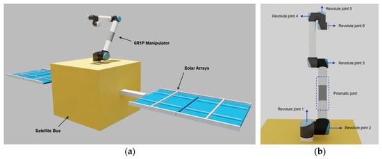
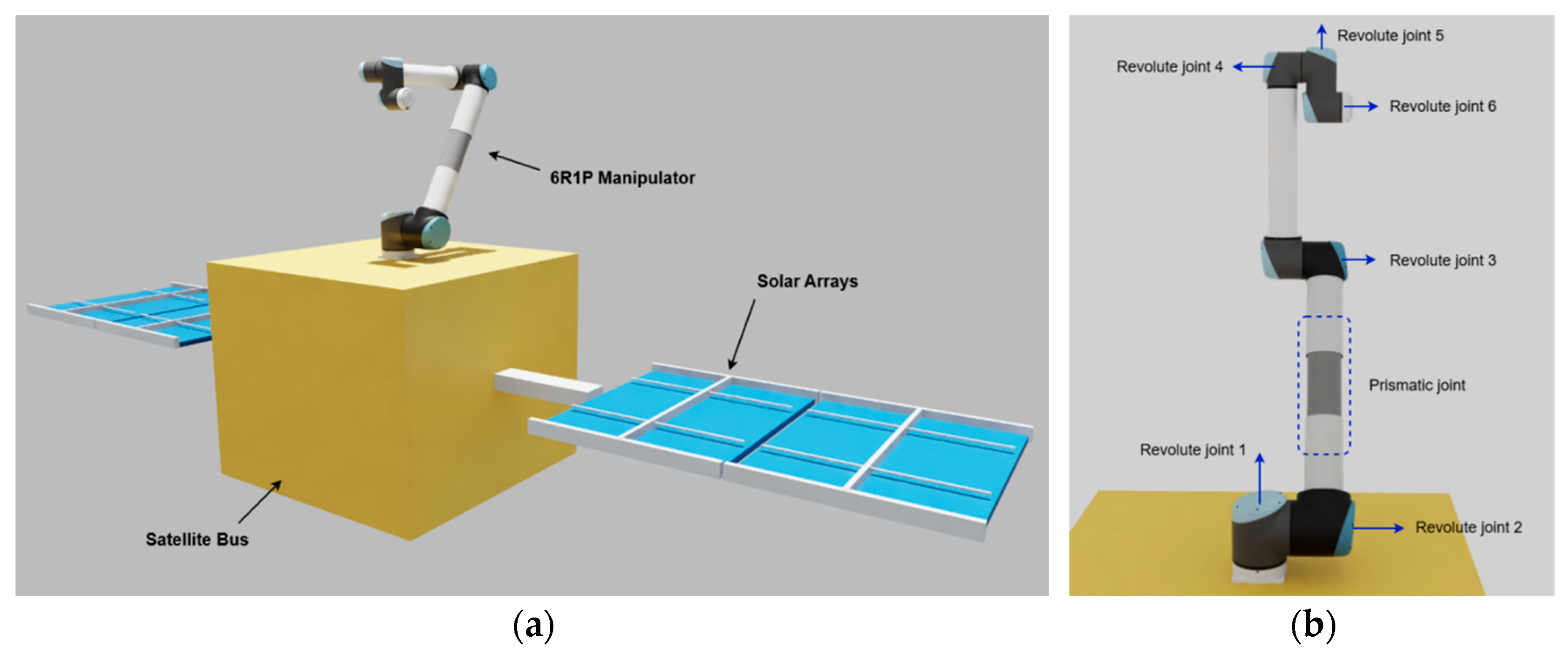
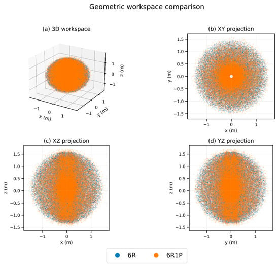
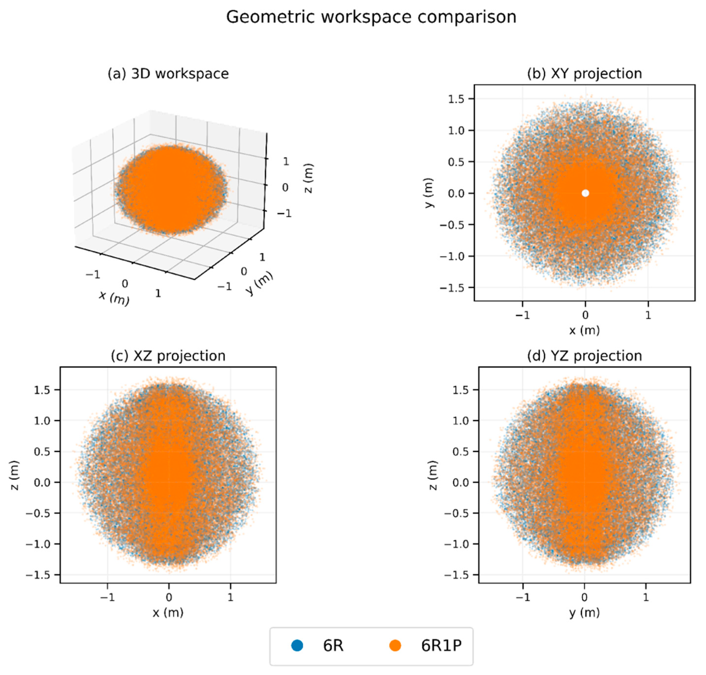
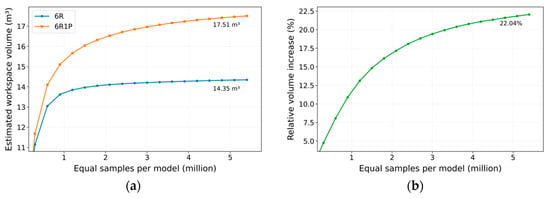
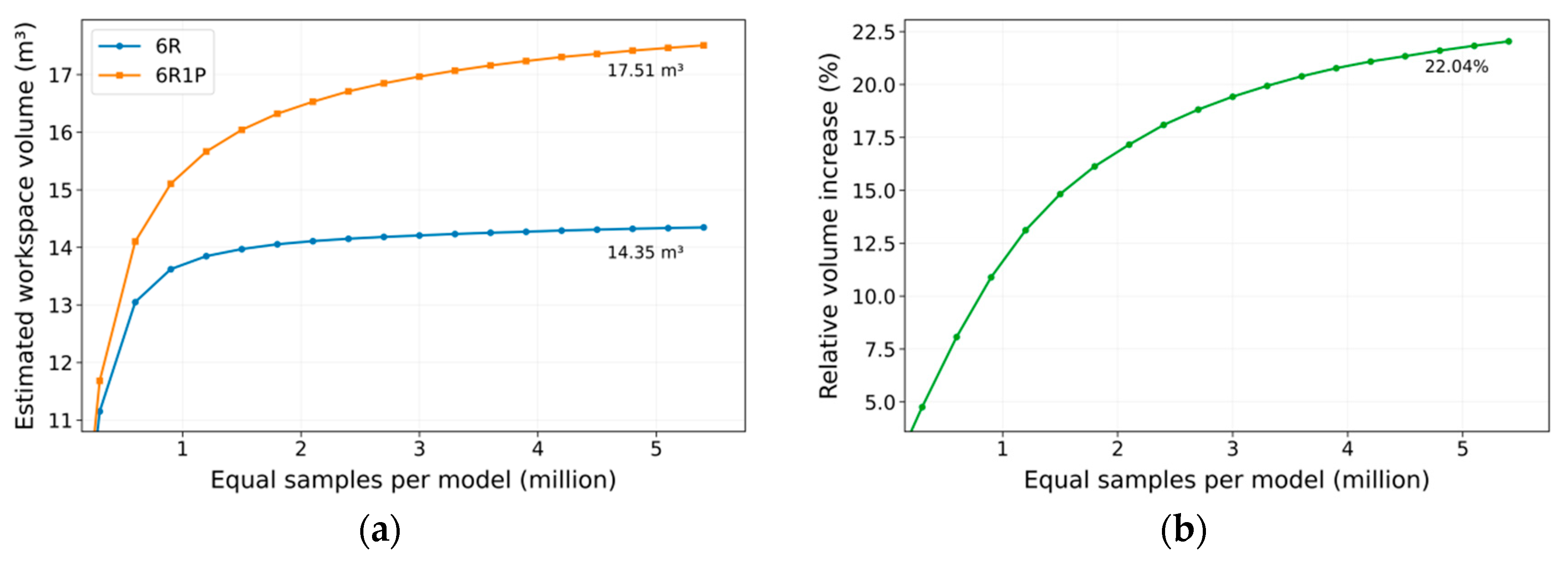
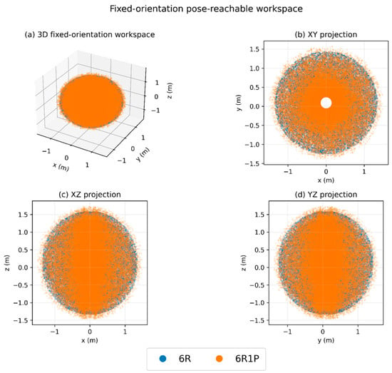
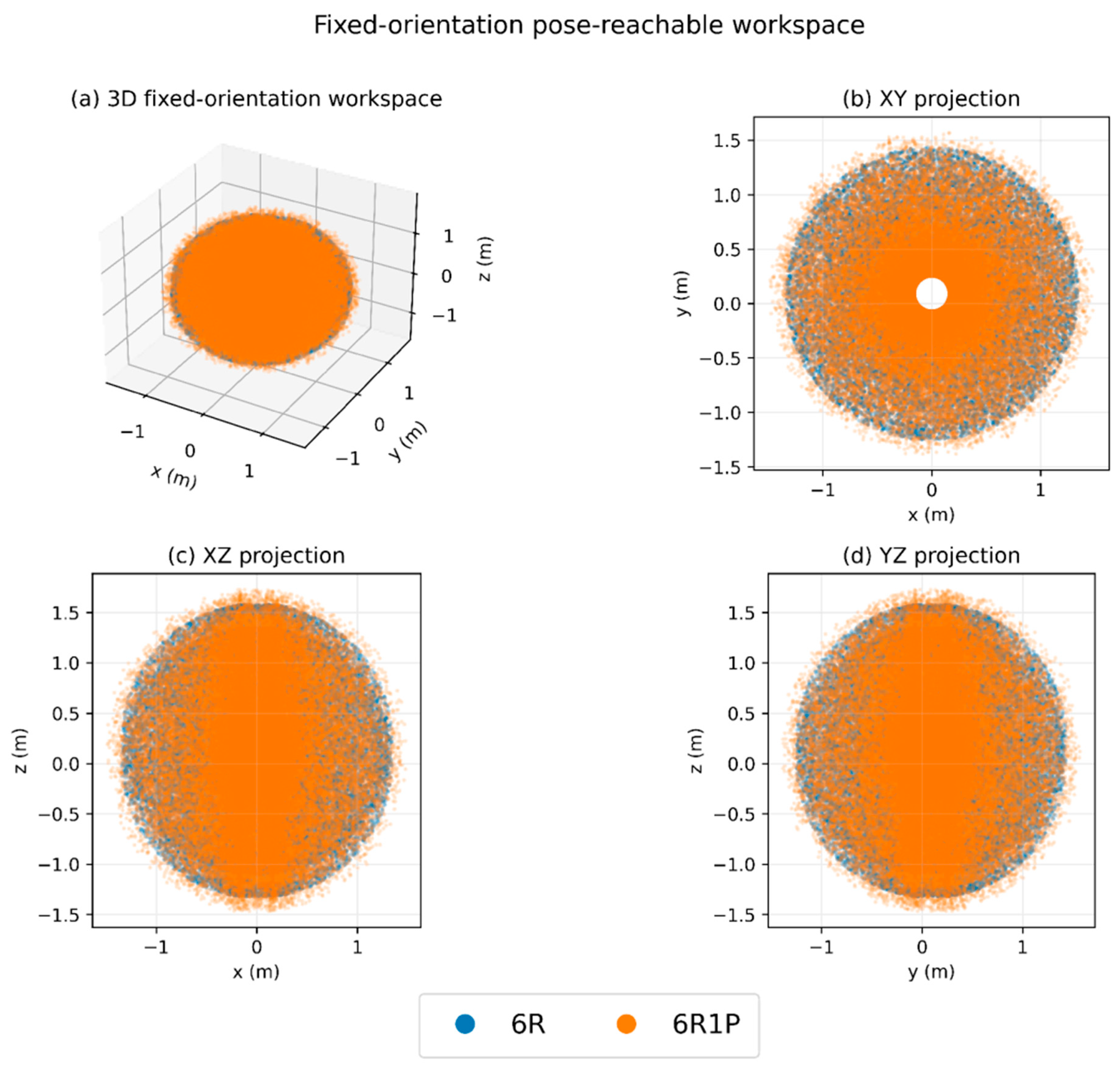
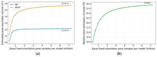
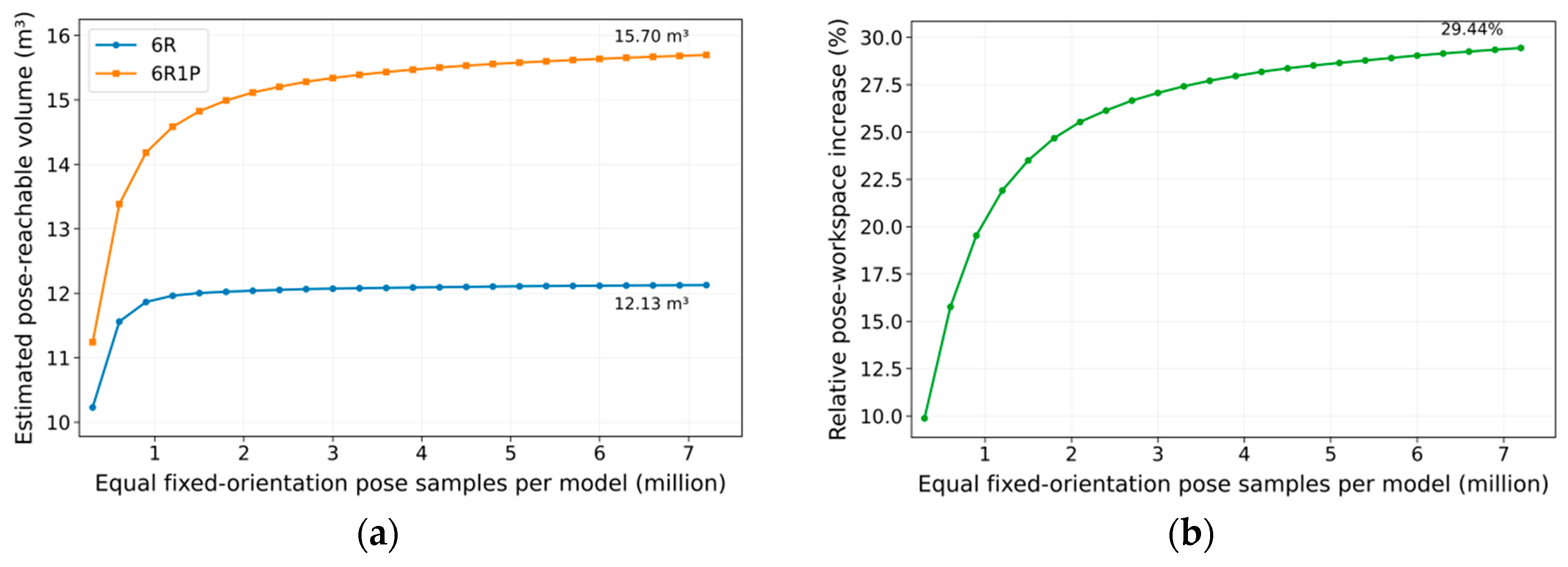
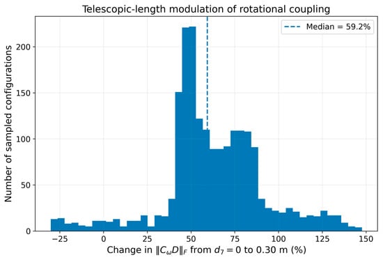
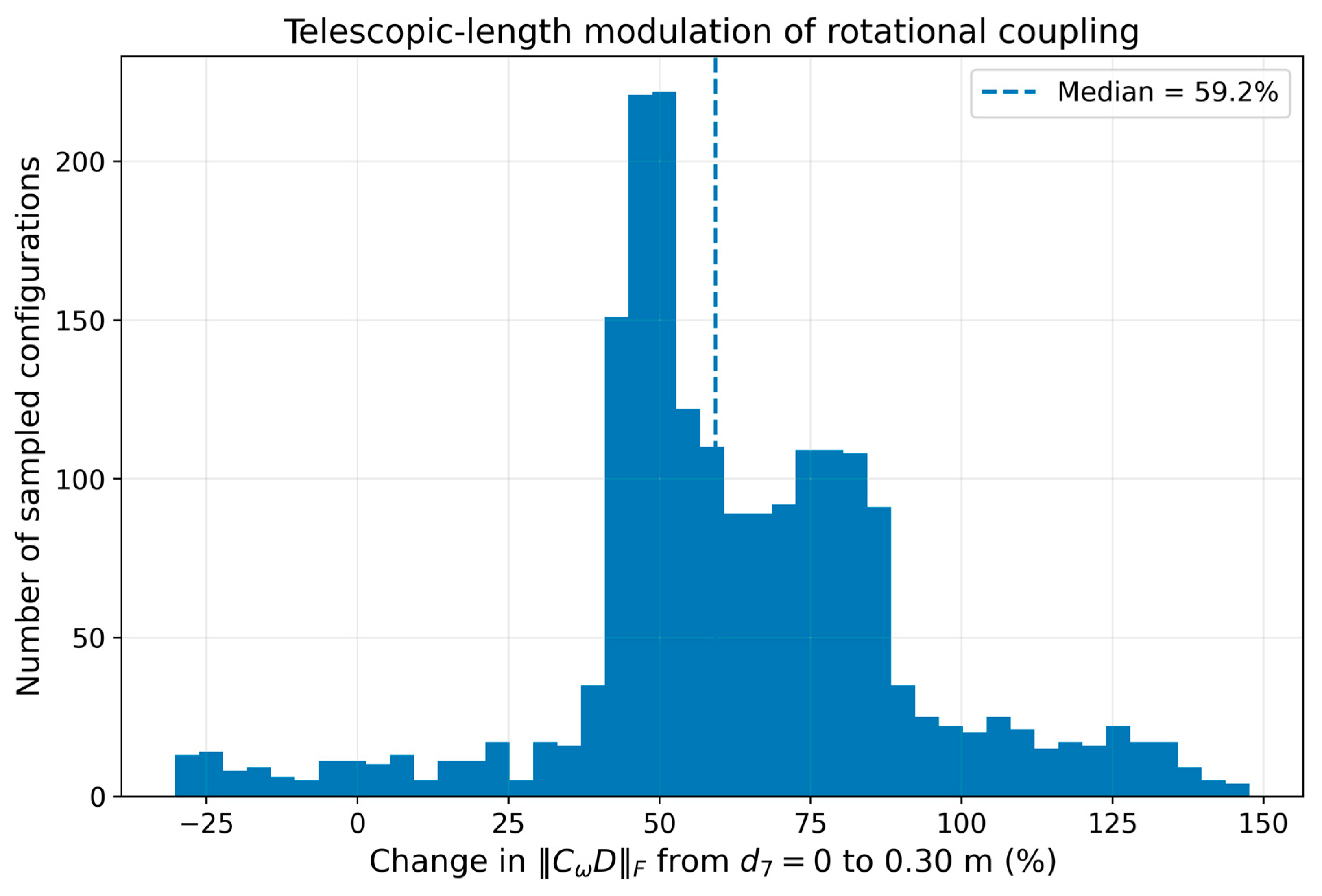
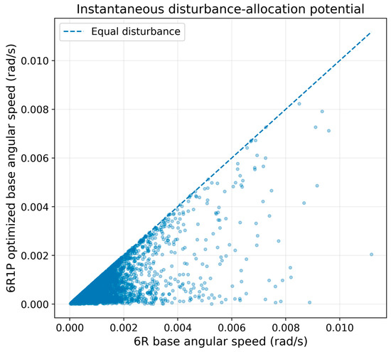
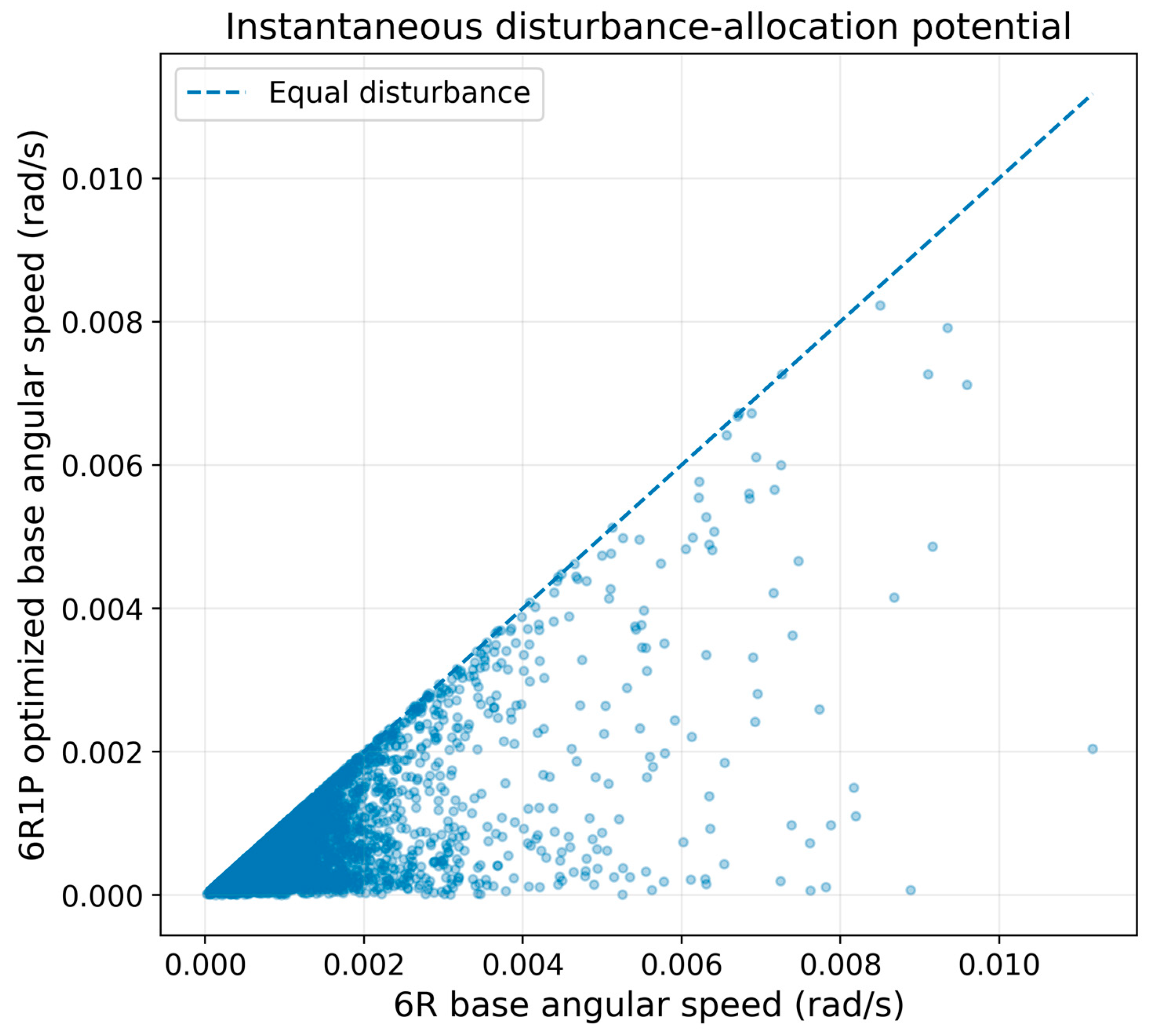
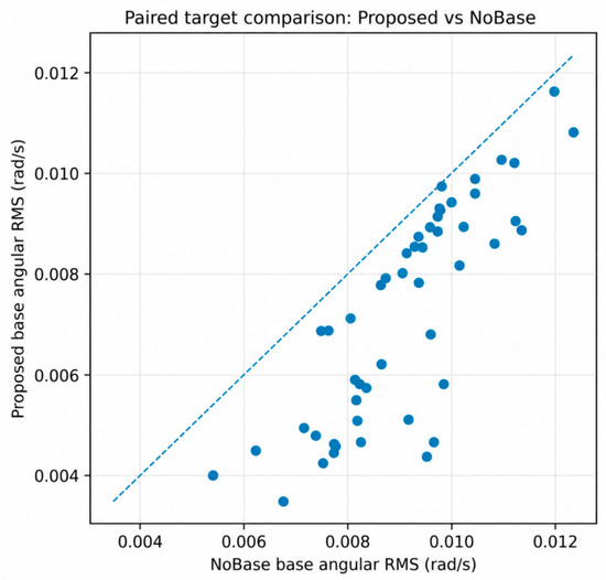
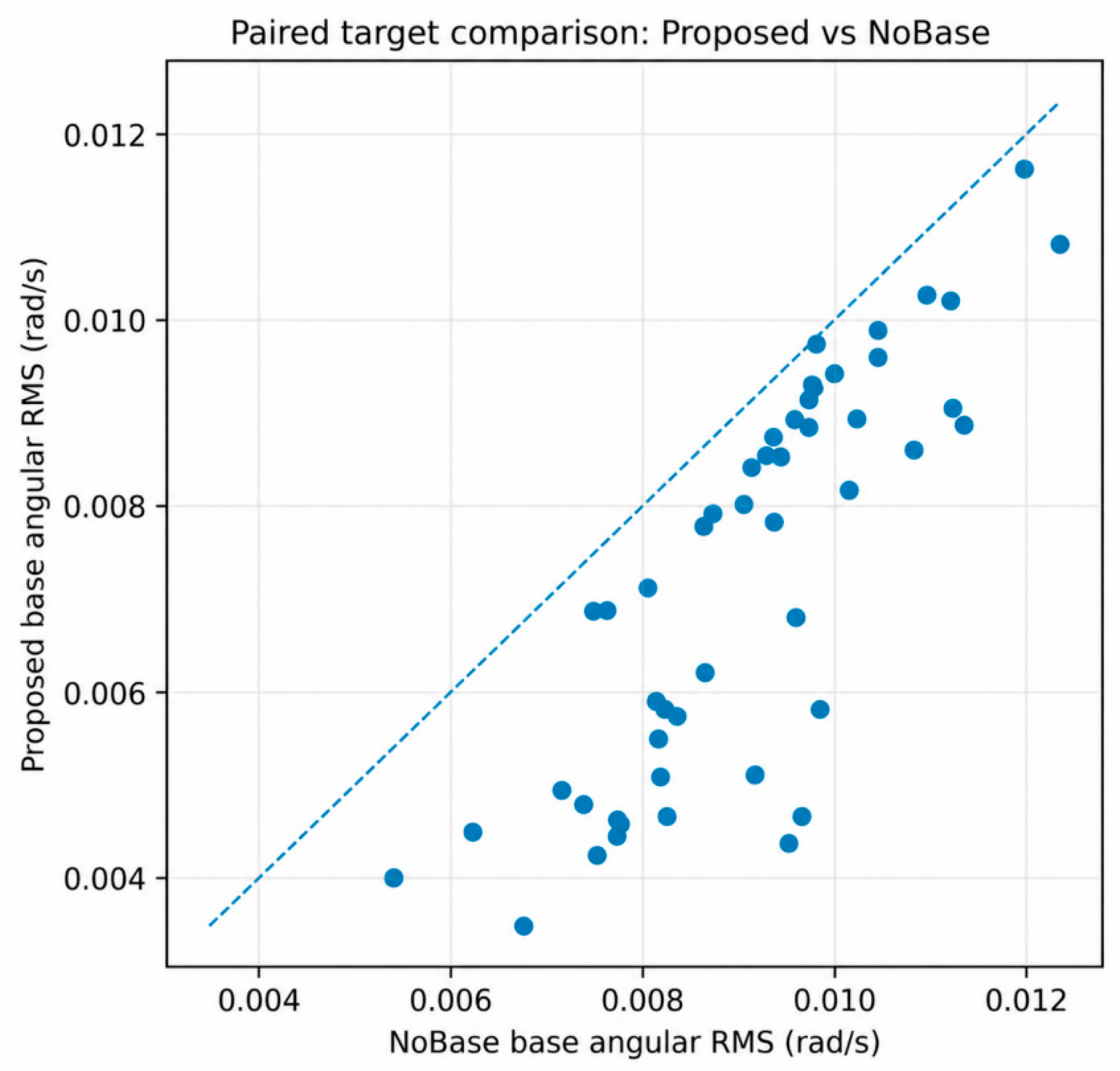
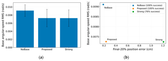
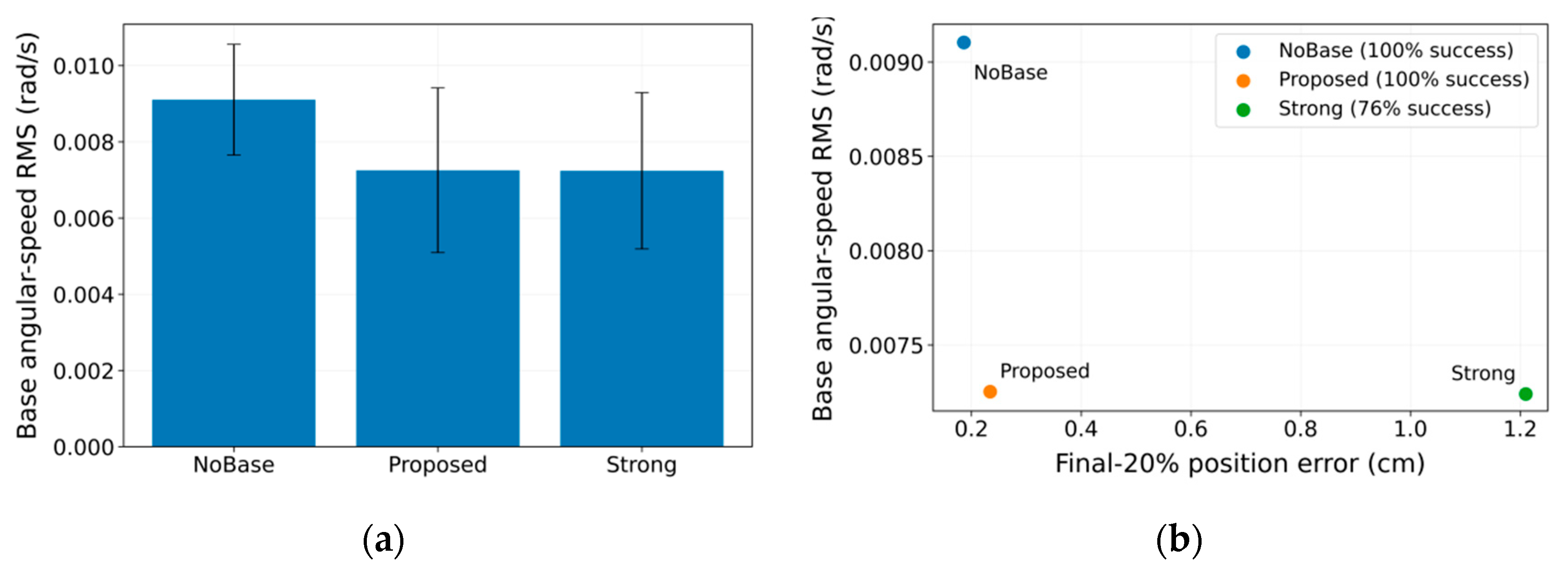
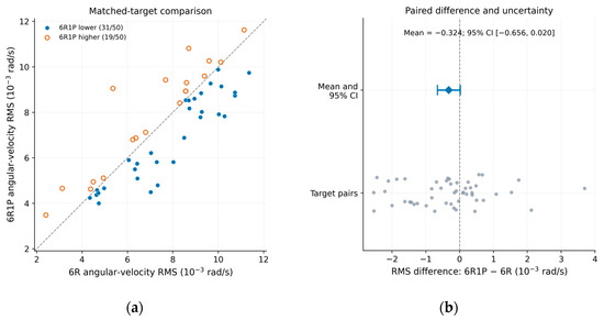
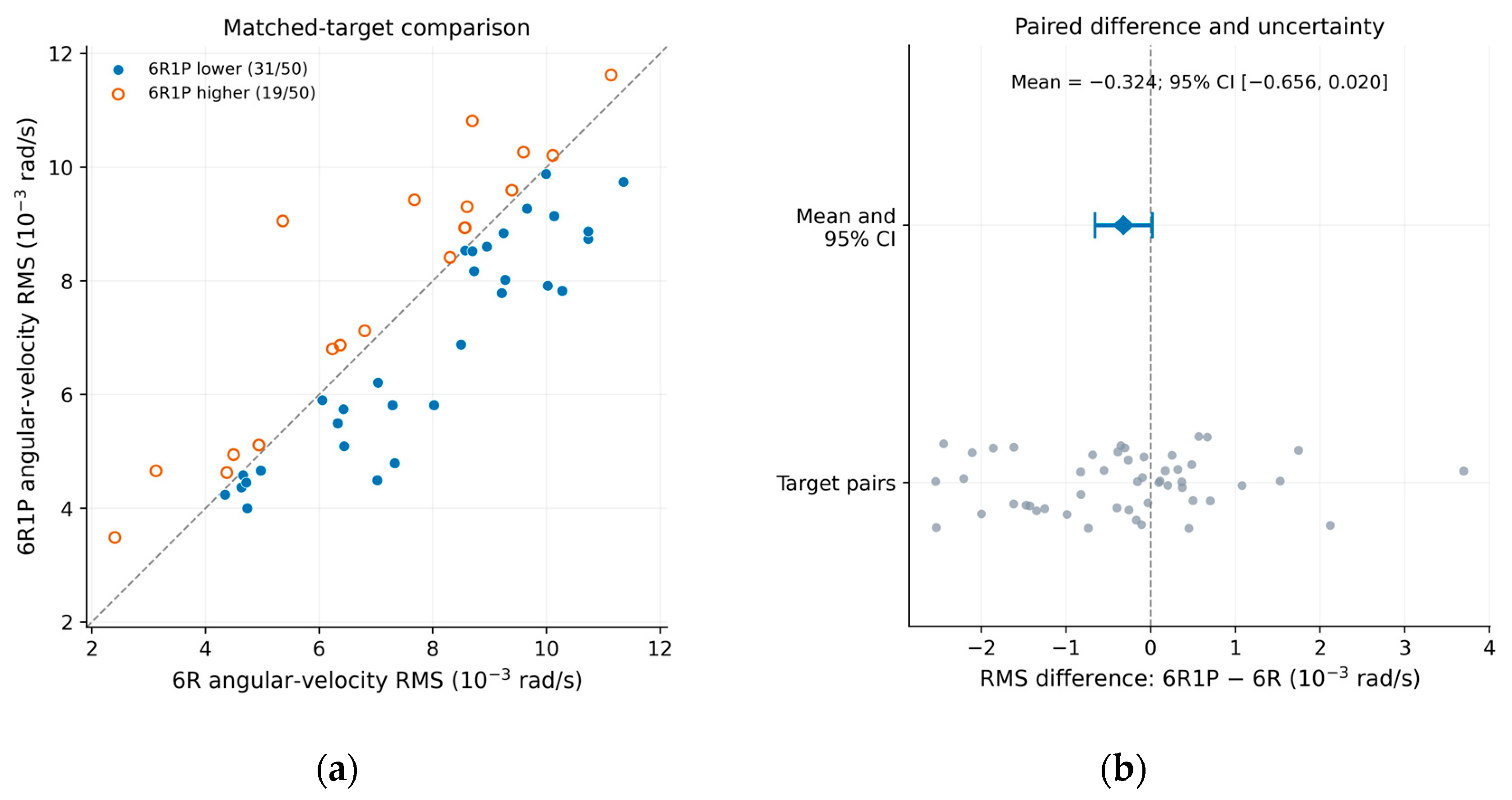
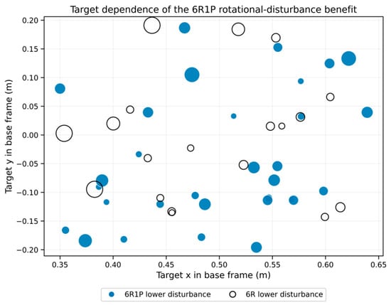
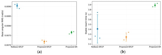
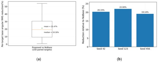
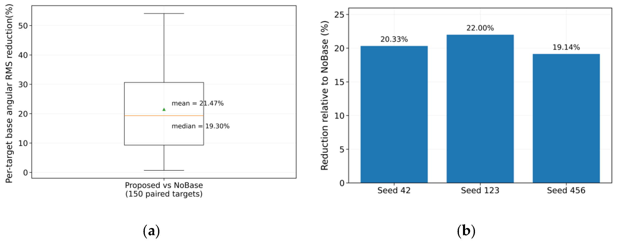
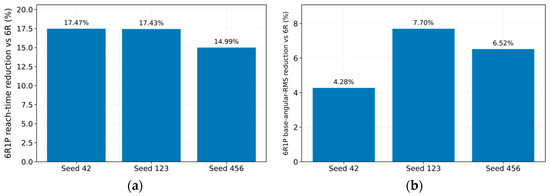
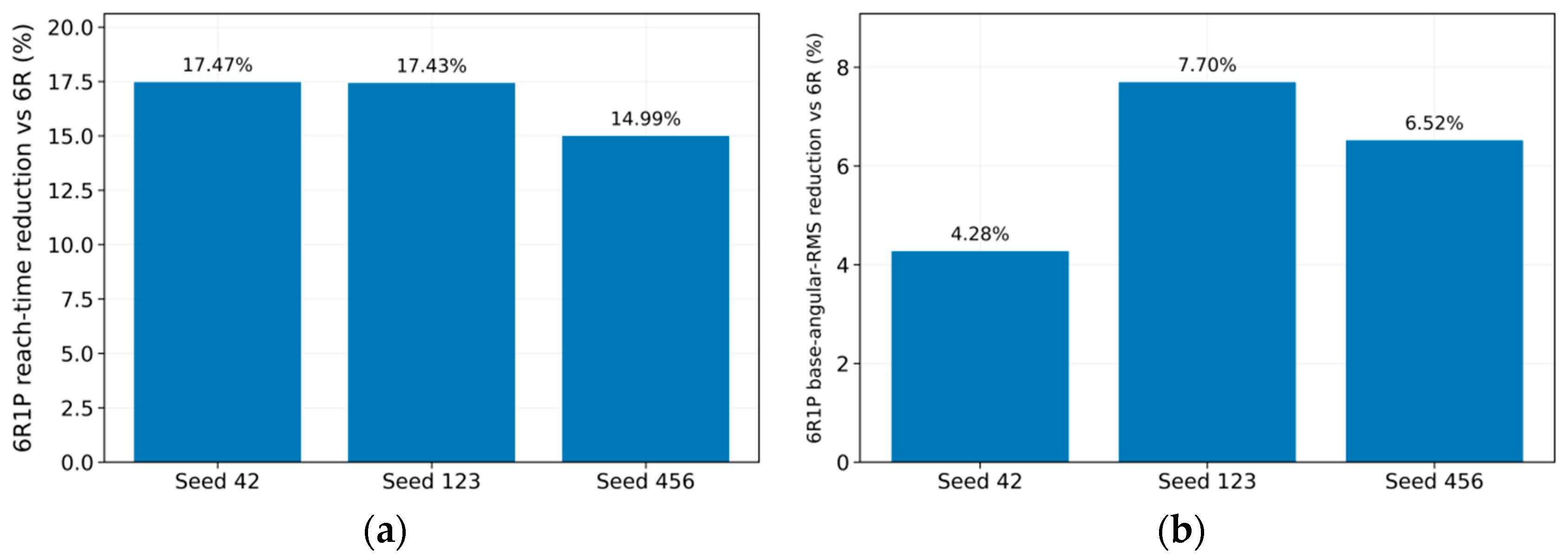
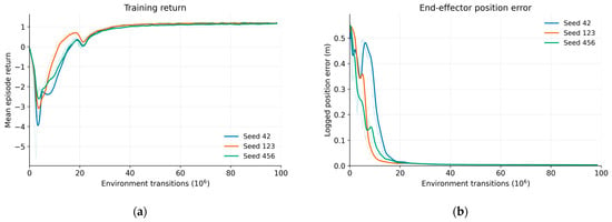
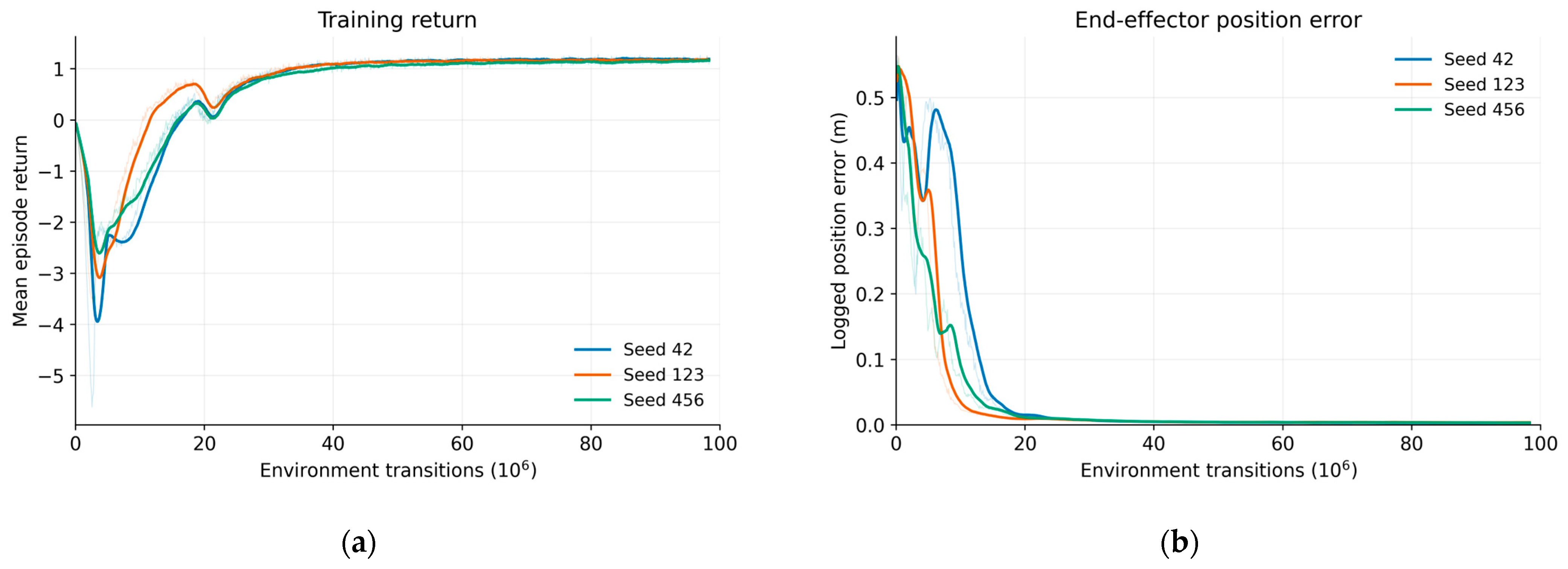
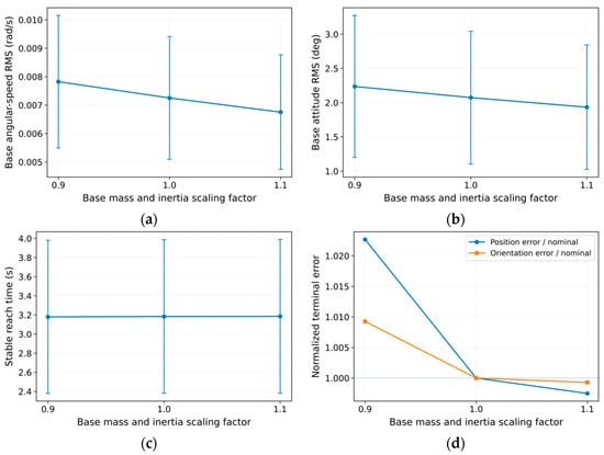
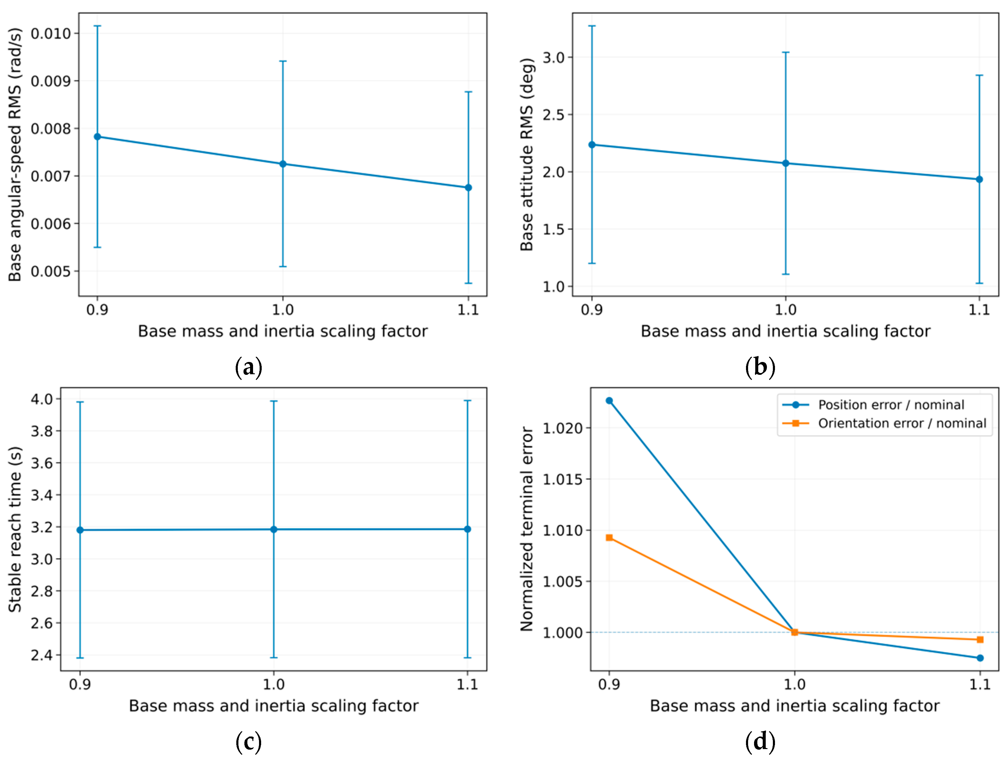
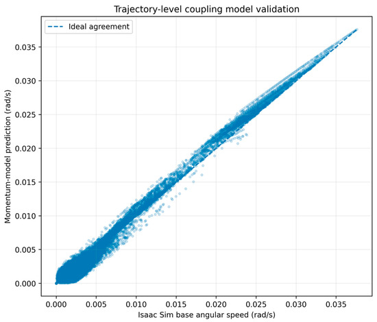
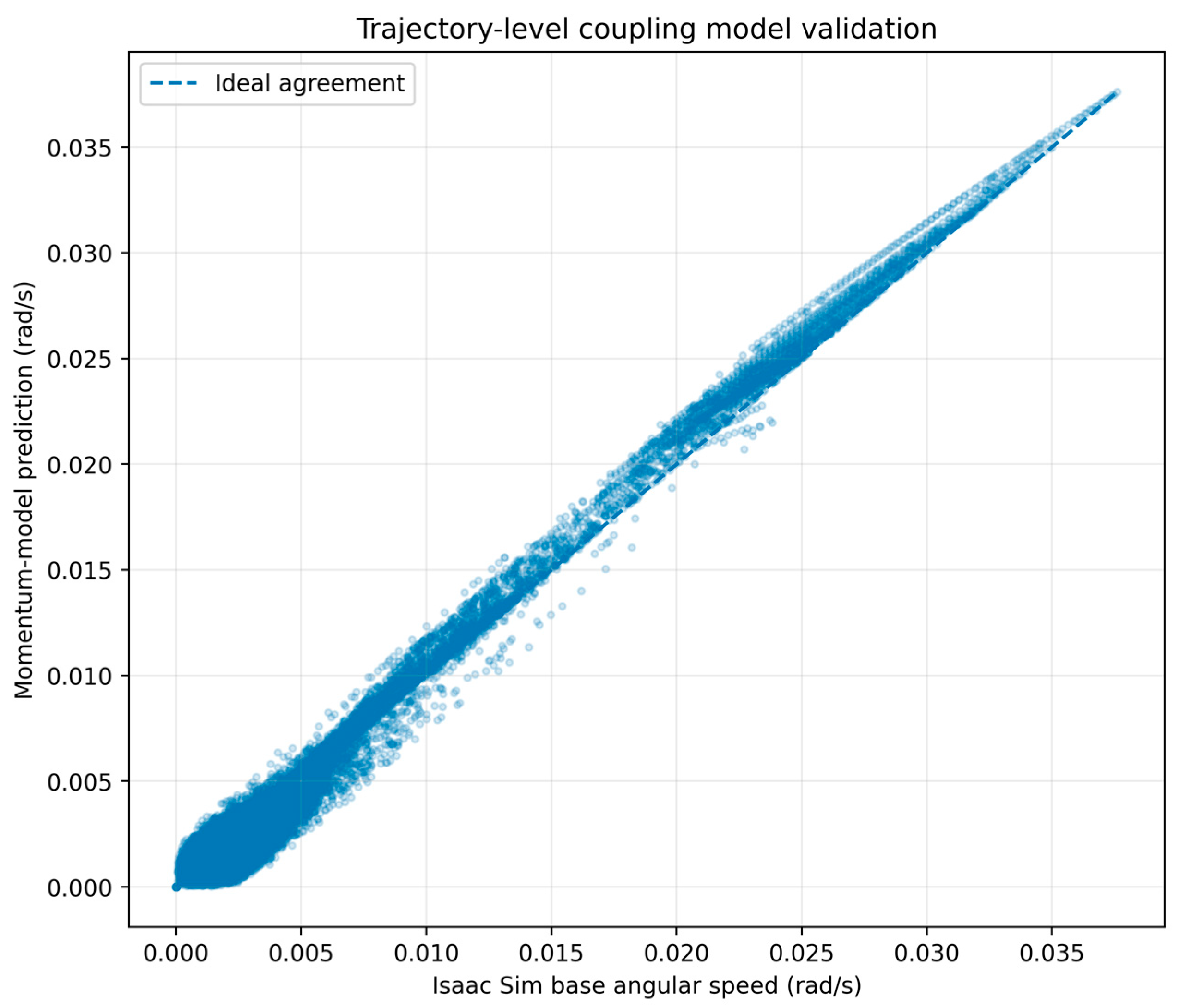
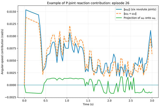
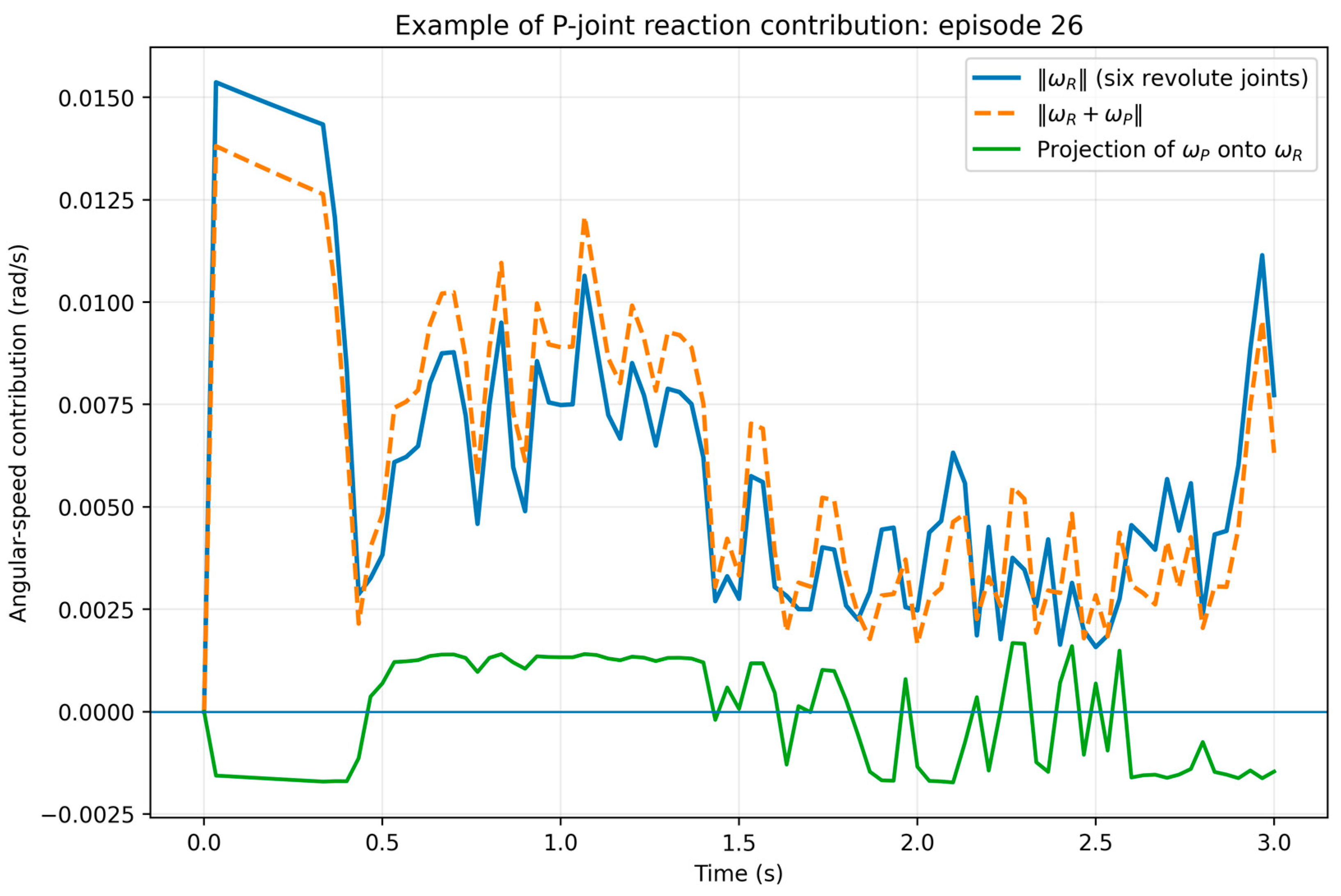
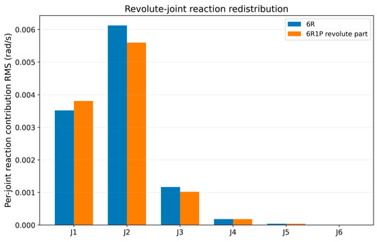
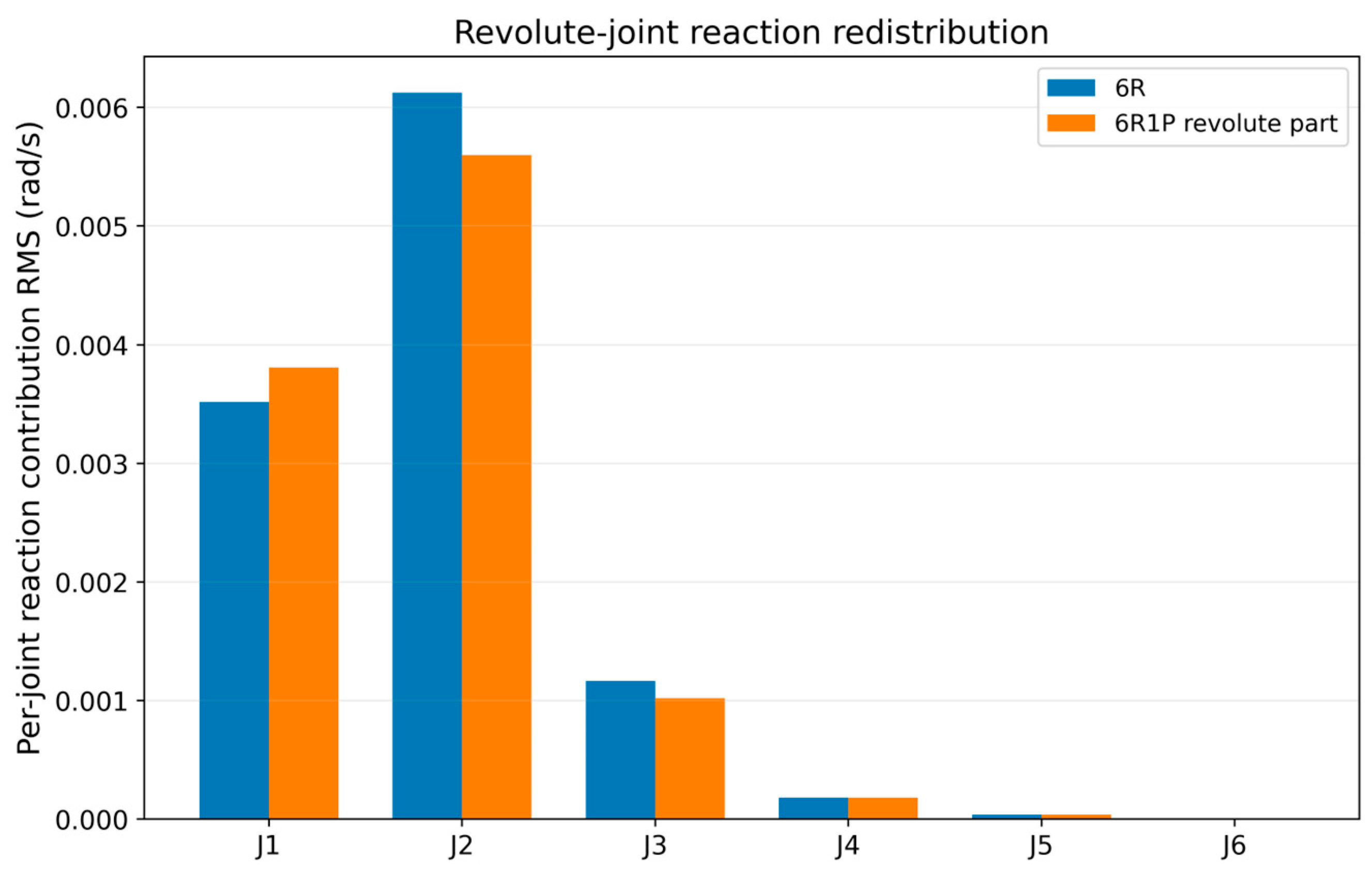
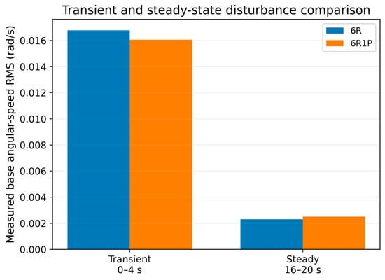
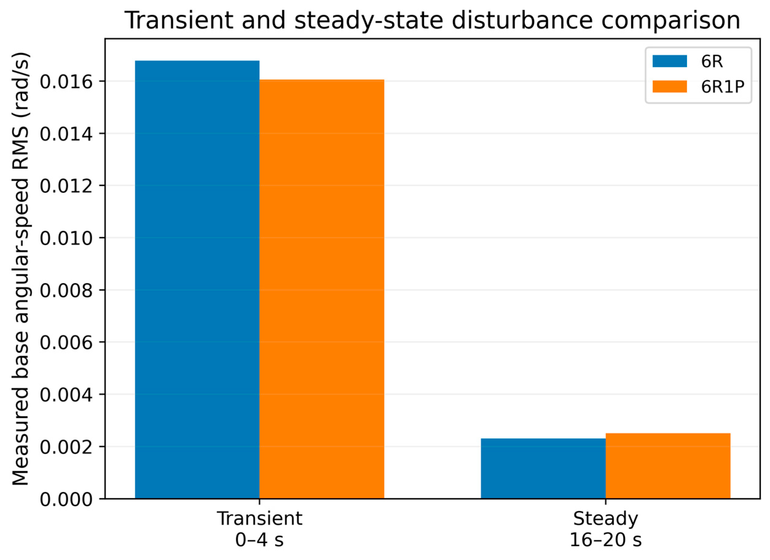

Disclaimer/Publisher’s Note: The statements, opinions and data contained in all publications are solely those of the individual author(s) and contributor(s) and not of MDPI and/or the editor(s). MDPI and/or the editor(s) disclaim responsibility for any injury to people or property resulting from any ideas, methods, instructions or products referred to in the content. |
© 2026 by the authors. Licensee MDPI, Basel, Switzerland. This article is an open access article distributed under the terms and conditions of the Creative Commons Attribution (CC BY) license.