


Abstract
Accurate remaining useful life (RUL) prediction of rolling bearings is important for condition-based maintenance. This study proposes an interpretable rolling RUL prediction framework integrating adaptive multidomain degradation representation, prognostic-stage localization, and differential Gaussian process regression (Diff-GPR). A 48-dimensional feature pool is extracted from six vibration domains, and bearing-specific degradation-sensitive subsets are selected using monotonicity, trendability, robustness, and redundancy criteria. The retained features are directionally aligned, percentile-normalized, equally fused, and smoothed to construct a fusion virtual health indicator (Fusion-VHI). A two-stage localization strategy identifies sustained degradation onset and the subsequent prediction-ready point, after which Diff-GPR models multiscale degradation increments and recursively updates failure time and RUL. The framework was evaluated on all 15 bearings from the Xi’an Jiaotong University–Changxing Sumyoung Technology (XJTU-SY) dataset and all 17 bearings from the 2012 Prognostics and Health Management (PHM2012)/PRONOSTIA dataset. Full final rolling prediction coverage was achieved, with mean absolute error/root-mean-square error (MAE/RMSE) values of 6.33/7.26 min on XJTU-SY and 6.03/6.98 min on PHM2012, and overall values of 6.17/7.11 min. Representative 99% predictive intervals achieved 100% prediction-interval coverage probability, while signed-error analysis identified 13 early and 19 late final predictions with an overall mean signed error of +1.77 min.
1. Introduction
Rolling bearings are key components of rotating machinery and are widely used in manufacturing, transportation, wind turbines, and power-generation systems. Bearing degradation can increase vibration, reduce operating accuracy, cause unplanned shutdowns, and damage nearby components. Accurate remaining useful life (RUL) prediction is therefore important for condition-based maintenance and prognostics and health management [1,2]. Prognostics and health management (PHM) provides a systematic framework for monitoring degradation, assessing system health, and forecasting future failure to support proactive maintenance decisions [3]. RUL is the operating time from the current observation to a specified failure threshold [1,4]. Unlike fault diagnosis, RUL prediction must infer future degradation from incomplete and uncertain observations. Run-to-failure datasets such as XJTU-SY support the development and evaluation of bearing prognostic methods under different operating conditions [5]. Reliable RUL prediction requires an informative degradation representation, an appropriate prediction stage, and accurate trajectory extrapolation.
Feature-based data-driven methods retain explicit degradation variables and provide an interpretable link between vibration signals and health assessment. Javed et al. [6] transformed multidimensional vibration measurements into a prognostic health representation. Guo et al. [7] combined time–frequency and related-similarity features, selected degradation-sensitive variables, and constructed an RNN-based health indicator. Xu et al. [8] proposed an unsupervised method for constructing health indicators. Recent studies have also used nonlinear feature selection [9] and multilevel dynamic evaluation with uncertainty modeling [10]. These studies show the importance of feature evaluation and health-indicator construction, but a preset feature set, dimensionality, or fusion rule may not suit all bearing degradation trajectories.
Deep learning can learn nonlinear degradation patterns and temporal dependencies from raw vibration signals or feature sequences—early studies combined autoencoders, deep neural networks, and convolutional models [11,12]. Recent work has examined Transformer, BiLSTM, TCN, transfer learning, attention, and graph-based models [13,14,15,16,17,18,19,20,21,22,23,24,25]. These models can capture complex patterns, but their performance depends on the available run-to-failure data, network design, hyperparameters, and computing resources.
Statistical and other non-deep-learning methods offer a more transparent route for degradation modeling and trajectory extrapolation. Si et al. [4] reviewed statistical RUL methods based on stochastic processes, filtering, and regression. Gaussian process regression (GPR) models nonlinear functions and provides predictive means and variances [26]. Previous studies have applied composite-kernel GPR [27], integrated GPR [28], and adaptive ensemble GPR [29] to bearing prognosis. Nonlinear Wiener process models [30] and trajectory similarity methods [31] have also been studied. However, their performance depends on the degradation representation and on the length and maturity of the observed segment. A fixed feature number or fusion rule may not suit bearing-specific trajectories, while a short or noisy segment can produce an unreliable degradation rate. These limitations motivate adaptive degradation representation, prediction-stage localization, and regularized increment-based extrapolation.
Recent developments in vibration-based condition monitoring and structural health monitoring (SHM) have further emphasized the importance of informative and interpretable signal representations. Civera and Surace [32] reviewed non-destructive techniques for condition monitoring and SHM and highlighted the importance of damage-sensitive vibration information for machinery and structural assessment. Civera et al. [33] introduced Teager–Kaiser energy cepstral coefficients as effective vibration-based damage-sensitive features for SHM applications. In rolling-bearing diagnosis, Spirto et al. [34] combined symmetrized-dot-pattern indices with a feedforward neural network for fault detection, while Chen et al. [35] developed an interpretable wavelet Kolmogorov–Arnold convolutional LSTM for spatial–temporal fault-feature extraction. Although these studies mainly address condition monitoring and fault diagnosis rather than RUL prediction, they further demonstrate the importance of robust, degradation-sensitive, and interpretable vibration representations for machinery health assessment.
Based on the above considerations, this study develops an interpretable framework for rolling-bearing RUL prediction by integrating adaptive multidomain degradation representation, prediction-stage localization, and rolling differential Gaussian process regression (Diff-GPR). The main contributions of this study are summarized as follows:
(1) An adaptive multidomain feature-selection and fusion method is developed to construct a degradation-sensitive health indicator while reducing the influence of redundant vibration features and accommodating bearing-specific degradation characteristics.
(2) A two-stage prognostic localization strategy is established to identify persistent departure from the healthy state and subsequently determine when sufficient degradation information has accumulated for reliable RUL modeling.
(3) A rolling differential Gaussian process regression (Diff-GPR) method is developed to model multiscale degradation increments rather than directly extrapolating the absolute health-indicator level, enabling the degradation trajectory and RUL estimate to be progressively updated as new observations become available.
The proposed framework is evaluated on the XJTU-SY and PHM2012 run-to-failure bearing datasets. In addition to conventional RUL prediction errors, rolling-stage prediction performance, prediction coverage, uncertainty, and comparative results are examined to provide a broader assessment of the proposed method.
The remainder of this paper is organized as follows. Section 2 introduces the XJTU-SY and PHM2012 datasets and the associated data-preprocessing procedures. Section 3 presents the adaptive Fusion-VHI construction, prognostic-stage localization, and rolling Diff-GPR methodology. Section 4 reports the experimental results and comparative analyses. Section 5 discusses the principal findings and limitations, and Section 6 concludes the paper and outlines directions for future work.
2. Materials
2.1. XJTU-SY Bearing Dataset and Evaluation Protocol
The Xi’an Jiaotong University–Changxing Sumyoung Technology (XJTU-SY) accelerated life-test dataset was used as the first experimental dataset [5]. It contains complete run-to-failure vibration measurements from 15 LDK UER204 rolling bearings tested under three operating conditions, with five bearings assigned to each condition. Figure 1 shows the XJTU-SY test rig used in the accelerated life tests. The three operating conditions differ in rotational speed and radial load, as summarized in Table 1.
Figure 1.
XJTU-SY bearing experimental platform: (a) overall view of the test rig, (b) close-up view of the bearing test section with accelerometers.
Table 1.
Main operating conditions of the XJTU-SY bearing dataset.
During each life test, vibration signals were acquired at a sampling frequency of 25.6 kHz. Each vibration record contains 32,768 sampling points, corresponding to an acquisition duration of 1.28 s, and successive records were collected at intervals of 60 s. The complete chronological sequence of each bearing was retained for degradation-feature extraction, health-indicator construction, FPT localization, and rolling RUL evaluation.
Two orthogonal vibration channels are available in the dataset. In the present study, the first vibration channel was used consistently for all bearings so that the feature-extraction and prognostic procedures were applied under a unified input configuration.
2.2. PHM2012 Bearing Dataset
To evaluate the generalization of the proposed framework on a second public run-to-failure dataset, the PHM2012 bearing dataset collected using the PRONOSTIA experimental platform was additionally employed. The experimental platform is illustrated in Figure 2. The dataset contains 17 bearings tested under three combinations of rotational speed and radial load, as summarized in Table 2. Condition 1 contains seven bearings operated at 1800 rpm under a radial load of 4000 N, Condition 2 contains seven bearings operated at 1650 rpm under 4200 N, and Condition 3 contains three bearings operated at 1500 rpm under 5000 N.
Figure 2.
PHM2012 bearing experimental platform.
Table 2.
Main operating conditions of the PHM2012 bearing dataset.
The vibration signals were sampled at 25.6 kHz. Each acquisition record contains 2560 samples per vibration channel, corresponding to an acquisition duration of 0.1 s, and successive records were acquired at intervals of 10 s. Two orthogonal acceleration channels are available together with the acquisition-time information. As for XJTU-SY, the first vibration channel was used consistently throughout the present study.
All 17 available complete bearing trajectories were included in the analysis. No bearing was removed according to its final RUL prediction error. Bearings for which the subsequent FPT or prediction-point criteria could not be satisfied were retained in the dataset and reported as ineligible for the corresponding downstream RUL evaluation rather than being replaced by fallback predictions.
2.3. Data Organization and Preprocessing
For each bearing, the vibration records were arranged according to their acquisition sequence before subsequent analysis. The horizontal vibration component was consistently adopted for all bearings in both datasets to maintain a unified input configuration.
The original vibration signals of both datasets were sampled at 25.6 kHz. Prior to multidomain feature extraction, an eighth-order Chebyshev Type I anti-aliasing filter with a passband ripple of 0.05 dB was applied using zero-phase filtering, after which the signals were downsampled by a factor of four. The effective sampling frequency was therefore reduced to 6.4 kHz. Consequently, each XJTU-SY vibration record contained 8192 samples after preprocessing, whereas each PHM2012 record contained 640 samples. The same preprocessing configuration was applied to all bearings and operating conditions. No variational mode decomposition was employed in the final preprocessing pipeline.
The original temporal spacing between successive vibration records was preserved. The acquisition interval is 60 s for XJTU-SY and 10 s for PHM2012. To ensure consistent temporal interpretation across the two datasets, subsequent smoothing and persistence-related operations were defined according to physical time rather than directly using a fixed number of observations. Thus, a duration of 300 s corresponds to five consecutive observations in XJTU-SY and 30 observations in PHM2012.
After preprocessing, each vibration record was converted into the multidomain feature representation described in Section 3.2. Signal-processing operations specific to individual feature families, including band-pass envelope analysis, Hilbert-envelope analysis, and stationary wavelet decomposition, are introduced together with the corresponding feature definitions in the following section.
3. Methods
3.1. Overall Framework of the Proposed Method
The proposed rolling-bearing remaining useful life prediction framework consists of three successive stages: multidomain degradation representation, prediction-stage localization, and rolling degradation extrapolation, as illustrated in Figure 3.
Figure 3.
Overall framework of the proposed RUL prediction method.
In the first stage, each vibration record is represented by a 48-dimensional multidomain feature vector containing time-domain, frequency-domain, Hilbert-envelope, time–frequency, band-pass-envelope, and envelope-spectrum descriptors. The resulting feature trajectories are evaluated according to their degradation sensitivity and mutual redundancy, and a bearing-specific subset is adaptively selected. The retained trajectories are directionally aligned, normalized to a common degradation scale, equally fused, and temporally smoothed to construct a scalar Fusion-VHI.
In the second stage, the Fusion-VHI is used to localize the prognostic process. The first prediction time (FPT) is determined by combining support vector data description (SVDD)-based novelty detection with statistical persistence confirmation. The subsequent prediction point Tp is defined according to the minimum amount of post-FPT degradation information required to initialize the multiscale differential regression model. Thus, the FPT characterizes persistent departure from the healthy operating region, whereas Tp represents model readiness for RUL prediction.
In the third stage, multiscale degradation increments are constructed from the observed Fusion-VHI segment and modeled using differential Gaussian process regression (Diff-GPR). The current degradation state and relative operating time are used to estimate future degradation increments, from which the future Fusion-VHI trajectory is recursively extrapolated. The predicted failure time is identified from the first crossing of the normalized failure threshold, and the corresponding RUL is updated as additional observations become available.
The three stages therefore provide a unified progression from vibration-based degradation representation to prognostic-stage localization and rolling RUL estimation.
3.2. Multidomain Feature Extraction
To characterize bearing degradation from complementary perspectives, a 48-dimensional multidomain candidate feature pool is constructed to describe variations in vibration amplitude, energy, impulsiveness, spectral distribution, envelope modulation, and time–frequency characteristics. The feature pool consists of 13 time-domain, eight frequency-domain, four Hilbert-envelope, four time–frequency, seven band-pass-envelope, and 12 envelope-spectrum features. These features are denoted as TD1–TD13, FD1–FD8, HE1–HE4, TF1–TF4, BP1–BP7, and ES1–ES12, respectively, as summarized in Table 3.
Table 3.
Composition of the 48-dimensional multidomain candidate feature pool.
The time-domain descriptors characterize waveform amplitude, dispersion, impulsiveness, and signal energy. They include the root-mean-square value, peak-to-peak value, variance, kurtosis, skewness, crest factor, shape factor, impulse factor, clearance factor, margin factor, energy, mean value, and standard deviation. The frequency-domain descriptors characterize the distribution and concentration of spectral energy and include spectral centroid, spectral spread, spectral skewness, spectral kurtosis, spectral entropy, dominant frequency, frequency center, and mean frequency.
To characterize amplitude-modulation behavior associated with bearing degradation, the analytic signal is obtained through the Hilbert transform, and its magnitude is taken as the vibration envelope. Four Hilbert-envelope descriptors are subsequently extracted, including envelope energy, entropy, peak value, and kurtosis.
Time–frequency information is obtained using a three-level stationary wavelet transform (SWT) with the Daubechies-4 wavelet. The corresponding descriptors consist of the first- and second-level detail-energy ratios, wavelet energy entropy, and the root-mean-square value of the approximation coefficients. No additional manual padding or truncation is introduced before SWT decomposition.
To emphasize modulation-related vibration components within the selected resonance band, an eighth-order Butterworth band-pass filter with a center frequency of 1000 Hz and a bandwidth of 500 Hz, corresponding to a passband of 750–1250 Hz, is applied in a zero-phase manner. Hilbert-envelope demodulation is subsequently performed on the filtered signal. Seven statistical descriptors, including envelope RMS, variance, kurtosis, skewness, crest factor, impulse factor, and entropy, are extracted from the resulting envelope.
The Fourier spectrum of the envelope signal is further used to construct 12 envelope-spectrum descriptors. These features characterize spectral position, dispersion, distribution shape, entropy, dominant components, signal energy, amplitude, and modulation-related spectral structure. Specifically, the envelope-spectrum feature group contains spectral centroid, spectral spread, spectral skewness, spectral kurtosis, spectral entropy, dominant frequency, spectral energy, peak value, RMS, mean value, the 50–150 Hz band-energy ratio, and the harmonic-energy ratio.
For bearing i, let Ni denote the number of vibration records in its run-to-failure sequence. The multidomain feature vector extracted from the t-th vibration record is defined as
where fi,j(t) denotes the value of the j-th candidate feature extracted from the t-th vibration record of bearing i. By arranging the feature vectors in chronological order, the complete run-to-failure feature matrix of bearing i is expressed as:
Each row of corresponds to one vibration record, whereas each column represents the temporal trajectory of one candidate degradation feature. The resulting feature matrix is then used for degradation-sensitivity evaluation and for bearing-specific feature-subset selection.
3.3. Degradation-Sensitive Feature Selection
The 48 candidate features exhibit substantially different sensitivities to bearing degradation. Some feature trajectories show persistent long-term evolution, whereas others are dominated by short-term fluctuations or contain information that is highly redundant with other descriptors. Therefore, a bearing-specific feature-selection procedure is employed to jointly consider degradation sensitivity and inter-feature redundancy. The procedure consists of degradation-sensitivity evaluation, adaptive determination of the feature-subset dimension, and redundancy-aware subset selection.
3.3.1. Degradation-Sensitivity Evaluation
Before degradation-sensitivity evaluation, each candidate feature trajectory is smoothed using an exponentially weighted moving average (EWMA) with a span of five observations. The same smoothing span is used for feature assessment in both datasets. This operation is intended to suppress short-term fluctuations during feature evaluation and is distinct from the physical-time smoothing subsequently applied to the final Fusion-VHI. For the jj-th candidate feature of bearing ii, the smoothed trajectory is defined as:
where
Here, fi,j(t) and denote the raw and EWMA-smoothed feature values, respectively. Three complementary indicators, namely monotonicity, trendability, and robustness, are then used to characterize the degradation sensitivity of each candidate feature.
Monotonicity evaluates the directional consistency of the smoothed feature trajectory. Let ni,j+ and ni,j− denote the numbers of positive and negative adjacent increments in , respectively. The monotonicity score is defined as:
Zero increments contribute to neither ni,j+ nor ni,j−. A larger Moni,j therefore indicates a more persistent unidirectional tendency over the run-to-failure trajectory.
Trendability measures the long-term association between the smoothed feature trajectory and operating progression. Let denote the observation-index vector. The trendability score is defined as:
where denotes the Pearson correlation coefficient and denotes the complete smoothed trajectory of the j-th feature. The absolute correlation is adopted because both increasing and decreasing trajectories can provide degradation information.
The sign of the same Pearson correlation is retained separately as the degradation-direction coefficient,
Features with zero degradation direction are excluded from subsequent selection. For the retained features, di,j∈{−1,+1}, and the direction coefficient is subsequently used to align the selected trajectories such that larger values consistently correspond to more severe degradation.
Robustness quantifies the resistance of a feature trajectory to short-term deviations from its smoothed degradation tendency. It is defined as:
where the data-scaled denominator floor is:
The adaptive denominator floor prevents numerical instability when the instantaneous feature magnitude approaches zero. A larger robustness value indicates that the raw trajectory remains closer to its underlying smoothed tendency.
Because the numerical distributions of Mon, Tre, and Rob may differ, the three metrics are further transformed into within-bearing percentile ranks. For X ∈ {Mon,Tre,Rob},
where denotes average ranking in the presence of tied values. The balanced degradation-sensitivity score of the j-th feature is then defined as the geometric mean of the three percentile measures:
The geometric mean penalizes features that perform strongly according to only one or two criteria but poorly according to another, thereby favoring more balanced degradation characteristics.
For a candidate feature subset S, its mean balanced degradation sensitivity is
For descriptive reporting and deterministic tie-breaking, the conventional composite degradation indicator is additionally defined as:
Importantly, KPIi,j is not used as a fusion weight in the final Fusion-VHI construction.
3.3.2. Adaptive Determination of the Subset Dimension
The number of retained degradation features is not predefined. After features with invalid degradation directions are excluded, the balanced degradation-sensitivity scores of the remaining valid candidates are used to identify the comparatively degradation-sensitive portion of the feature pool for each bearing.
Because the distributions of the balanced sensitivity scores may differ among bearings and may contain unusually high or low values, robust location and scale statistics are adopted instead of prescribing a fixed feature number. For bearing i, the median balanced degradation sensitivity is defined as:
and the corresponding median absolute deviation is:
The MAD is converted to a robust scale estimate using the conventional normal-consistency factor 1.4826:
A bearing-specific degradation-sensitivity threshold is then defined as:
Features whose balanced degradation-sensitivity scores exceed this threshold are regarded as comparatively degradation-sensitive candidates. The corresponding adaptive subset dimension is therefore:
This robust screening rule does not impose a predefined lower or upper bound on the number of retained features. Instead, Ki∗ reflects the number of candidate descriptors whose degradation sensitivity is distinctly higher than the typical level of the corresponding bearing. This step is particularly relevant to the subsequent equal-mean Fusion-VHI construction, because it limits the inclusion of weakly degradation-sensitive descriptors that could otherwise dilute the contribution of more informative features during fusion.
However, high degradation sensitivity alone does not guarantee complementary information. Therefore, the features retained by the robust sensitivity screening are not fused directly. Instead, they define the bearing-specific sensitivity level and subset dimension for the subsequent redundancy-aware optimization. To allow alternative complementary combinations around the high-sensitivity region, the reduced candidate pool is formed from the highest-ranked valid features:
where ni is the number of valid features after degradation-direction screening. All subsets containing Ki∗ features within these Li candidates are then evaluated according to the sensitivity-retention and NMI-based redundancy criteria described in Section 3.3.3. In this way, degradation-sensitive dimensionality determination and redundancy-aware feature-combination selection are treated as two successive but distinct steps.
3.3.3. Redundancy-Aware Subset Selection
High degradation sensitivity alone does not ensure that the selected features contain complementary information. Different amplitude-, energy-, and envelope-related descriptors may exhibit strongly dependent trajectories. To account for both linear and nonlinear dependence, normalized mutual information (NMI) calculated from rank-based quantile-discretized raw feature trajectories is used to quantify inter-feature redundancy.
For a candidate subset S, the mean pairwise redundancy is defined as:
When Ki∗ = 1, pairwise redundancy is undefined and redundancy optimization is therefore unnecessary; the highest-ranked valid feature is retained directly. For Ki∗ ≥ 2, the NMI-based subset-selection procedure described below is applied.
A smaller indicates lower average dependence among the selected feature trajectories.
Directly minimizing redundancy, however, may favor weakly degradation-sensitive features. Therefore, redundancy optimization is performed subject to a balanced-sensitivity retention criterion. At the selected dimension Ki∗, the maximum subset sensitivity is defined as:
where denotes the reduced candidate pool containing the Li highest-ranked valid features.
The sensitivity-feasible subset is then defined as:
Thus, only subsets retaining at least 95% of the maximum balanced sensitivity attainable at the selected dimension are considered for redundancy minimization. The final feature subset is obtained as
When numerically indistinguishable redundancy values occur, the candidate with higher degradation sensitivity is preferentially selected using the balanced-sensitivity and degradation-quality measures as deterministic tie-breaking criteria. Representative degradation-sensitivity ranking and NMI-based redundancy analysis results for the selected feature subsets are illustrated in Figure 4.
Figure 4.
Representative degradation-sensitivity ranking and redundancy analysis of the selected feature subsets. (a) Degradation-sensitivity ranking of the 48 candidate features for XJTU-SY Bearing1_1 and PHM2012 Bearing1_3, where only the top-ranked candidates are shown, colored bars denote the features retained in the final selected subset, and gray bars denote high-ranked candidates excluded after NMI-based redundancy optimization; (b) pairwise normalized mutual information (NMI) matrices of the selected feature subsets.
The resulting subset Si∗ therefore balances three considerations: degradation sensitivity, compact dimensionality, and inter-feature redundancy. In contrast to the previous score-weighted formulation, the degradation-sensitivity metrics are used only for feature assessment and subset determination and do not determine the contribution weights in the final health indicator. After Si∗ is obtained, the retained trajectories are directionally aligned, normalized using percentile-based scaling, and equally fused to construct the Fusion-VHI, as described in Section 3.4.
3.4. Fusion-VHI Construction
After the degradation-sensitive subset Si∗ has been determined, the selected feature trajectories are transformed into a scalar health indicator with a consistent degradation direction and comparable numerical scale. The Fusion-VHI construction consists of degradation-direction alignment, percentile-based scaling, equal-mean fusion, and temporal smoothing.
For the j-th selected feature of bearing i, the degradation-direction coefficient di,j obtained in Section 3.3 is first applied to align the trajectory:
where di,j∈{−1, +1}. After direction alignment, larger values of gi,j(t) consistently represent a more advanced degradation state, regardless of whether the original feature increases or decreases over the bearing lifetime.
To reduce differences in scale among heterogeneous feature families and limit the influence of extreme values, each aligned trajectory is transformed using its 5th and 95th percentiles. Let qi,j0.05 and qi,j0.95 denote the 5th and 95th percentiles of the complete raw direction-aligned trajectory gi,j(t), respectively. The normalized trajectory is defined as
This percentile-based transformation maps the central degradation range of each selected feature onto a common interval while preventing isolated extreme observations from disproportionately affecting the subsequent fusion.
Unlike the previous score-weighted formulation, the selected features contribute equally to the final degradation representation. For bearing i, the unsmoothed fused indicator is therefore defined as
where Ki∗ = ∣Si∗∣ is the adaptively determined number of selected features. Equal-mean fusion separates the roles of feature selection and feature aggregation: degradation-sensitivity scores determine which complementary features are retained, whereas no additional score-derived weighting is imposed after selection.
Because the acquisition intervals of XJTU-SY and PHM2012 are different, temporal smoothing is specified in physical time rather than by assigning the same observation span to both datasets. A smoothing duration of 300 s is adopted. This corresponds to an EWMA span of five observations for XJTU-SY, whose records are acquired every 60 s, and 30 observations for PHM2012, whose records are acquired every 10 s.
The final Fusion-VHI is recursively defined as
with
where
The initial value is set as
The resulting Vi(t) is referred to as the Fusion-VHI and is used in the subsequent degradation-stage localization and RUL prediction procedures. Its unified degradation direction ensures that larger values correspond to more severe degradation, while equal-mean fusion preserves complementary information from the adaptively selected feature subset without introducing additional feature-specific weighting parameters.
3.5. RBF-SVDD-Based First Prediction Time Determination
The first prediction time (FPT) is determined by identifying the onset of sustained degradation. To reduce the influence of isolated fluctuations, a persistence-constrained radial basis function support vector data description (RBF-SVDD) method is adopted. The conceptual principle of the RBF-SVDD detector is illustrated in Figure 5. Here, RBF denotes the radial basis function kernel, while SVDD denotes support vector data description.
Figure 5.
Conceptual principle of the RBF-SVDD detector. (a) Healthy Fusion-VHI reference constructed from the first 20 min; (b) implicit nonlinear mapping induced by the RBF kernel; and (c) calibrated SVDD healthy-state boundary. Blue circles represent healthy reference samples, whereas the red point denotes a candidate departure. A candidate departure is not directly regarded as the final FPT; the persistence criterion is subsequently applied.
For bearing i, the first 20 min of the Fusion-VHI sequence are used as the healthy reference. The Fusion-VHI is robustly standardized using the location and scale estimated from this reference:
where Vi(t) denotes the Fusion-VHI, ci and si are the robust location and scale parameters estimated from , and is a small numerical constant.
The nonlinear healthy-state distribution is characterized using an RBF kernel:
where is the kernel-width parameter and denotes the kernel-induced feature space.
The squared distance between a sample and the SVDD center is calculated by
where zij represents the standardized healthy reference samples and are the SVDD coefficients. The healthy-state boundary is calibrated from the healthy-reference distances.
The normalized departure score and the corresponding departure indicator are defined as
where is the calibrated healthy-boundary radius. Thus, ri(t) > 0 indicates a candidate departure from the healthy region.
To avoid treating an isolated abnormal observation as the FPT, a 300 s persistence window is applied. The FPT is defined as the endpoint of the first complete post-reference window containing at least ki departure observations:
where is the sampling interval and bi is the number of observations in the initial 20 min healthy reference. In this study, (ni,ki) = (5, 2) for XJTU-SY and (ni,ki) = (30, 5) for PHM2012.
This definition identifies the earliest statistically persistent departure from the healthy state rather than the first isolated abnormal observation. The subsequent prediction point Tp is determined separately according to the data-length requirement for rolling Diff-GPR prediction.
3.6. Prediction Point Determination
Although the FPT represents the estimated onset of sustained degradation, RUL prediction is not initiated directly at the FPT. First, the FPT is back-localized only after the subsequent Fusion-VHI evolution satisfies the sustained-degradation validation described in Section 3.5. Second, the multiscale Diff-GPR model requires a minimum amount of post-FPT degradation information to construct reliable increment samples. Therefore, a separate prediction point Tp is introduced to indicate the earliest stage at which the confirmed degradation segment contains sufficient information for subsequent RUL modeling.
The Diff-GPR model uses degradation increments over four temporal spans:
The longest span h = 8 provides relatively long-range local degradation information and is sampled with a stride of two observations. To ensure that this scale contributes a minimum of five increment samples, at least Ninit = 17 post-FPT observations are required. At this observation count, the available increment samples for h = 1,3,5, and 8 are 16, 14, 12, and 5, respectively. This requirement provides a common minimum information basis for initializing the multiscale differential model.
Because the sustained-degradation validation in Section 3.5 uses
and Nv,i ≥ Ninit, the validation requirement also guarantees that the minimum Diff-GPR initialization requirement has been satisfied. Let ji,FPT denote the record index of the localized FPT. The prediction point is therefore defined as
or, in physical time,
where Δti is the acquisition interval of the corresponding dataset.
For XJTU-SY, ni = 4, yielding Nv,i = 17; therefore, Tp occurs 16 min after the FPT. For PHM2012, ni = 24, yielding Nv,i = 48, corresponding to approximately 7.83 min after the FPT. Unlike the FPT, Tp does not represent an additional degradation-state transition. It only denotes the earliest prediction-ready point at which the sustained degradation episode has been confirmed and sufficient post-FPT information is available for initialization of the rolling Diff-GPR model.
3.7. Rolling Differential Gaussian Process Regression for RUL Prediction
3.7.1. Multiscale Differential Degradation Modeling
Directly extrapolating the absolute Fusion-VHI level is challenging because bearing degradation trajectories are generally nonstationary and may exhibit bearing-specific offsets, local plateaus, and different degradation rates. To reduce sensitivity to the absolute indicator level, the proposed method models local degradation increments rather than the Fusion-VHI itself.
Let V(t) denote the Fusion-VHI at observation t. For a temporal span h, the average degradation increment is defined as
To characterize degradation dynamics over different temporal scales, four spans are considered: . Short spans characterize local variations, whereas longer spans provide a smoother representation of the underlying degradation tendency. The multiscale targets are pooled to construct a unified regression dataset. In the primary formulation, positive increments are retained to characterize the forward degradation rate associated with progression toward the failure state. This choice introduces a directional modeling assumption and may suppress genuine local reversals or plateaus in the observed degradation trajectory; this limitation is discussed further in Section 5.
For each retained increment, the predictor uses the current degradation state together with relative operating time:
where τ(t) denotes the elapsed time relative to the available prediction history. Both input variables are standardized before Gaussian-process fitting.
3.7.2. Differential Gaussian Process Regression
Gaussian process regression is employed to characterize the relationship between the current degradation state and the subsequent degradation increment. The differential regression model is expressed as:
where denotes the latent degradation-increment function and represents the observation-noise variance.
A Matérn-5/2 covariance function is adopted because it allows less restrictive smoothness than the squared-exponential kernel and is therefore suitable for degradation trajectories containing gradual but locally varying dynamics. The covariance between two input samples is expressed as:
where , is the characteristic length scale, and represents the signal variance. For the training inputs , the latent covariance matrix is defined by:
Considering observation noise, the covariance matrix of the training targets is:
For a new input , the posterior predictive distribution of the degradation increment is:
with
and
The kernel hyperparameters are estimated by maximizing the log marginal likelihood. To restrict the optimization to numerically meaningful regions, the signal-scale parameter, Matérn length scale, and white-noise level are bounded within [0.05, 100], [0.1, 10], and [10−6, 0.1], respectively. Multiple optimizer initializations are used to reduce sensitivity to local optima.
The differential formulation differs fundamentally from direct level-GPR prediction. Absolute Fusion-VHI trajectories contain both the accumulated degradation state and bearing-specific trajectory offsets, making their long-term level distribution strongly nonstationary. By contrast, represents the local rate of degradation over a finite temporal interval. Conditioning these increments on the current Fusion-VHI and elapsed time removes part of the accumulated level effect and focuses the regression on local degradation dynamics. Consequently, the differential representation is expected to be less sensitive to absolute trajectory offsets and more suitable for recursive updating. This modeling rationale does not imply guaranteed empirical superiority over direct level-GPR. Rather, the differential formulation is adopted to reduce direct dependence on the accumulated absolute health-indicator level and to provide an increment-based representation suitable for recursive degradation extrapolation. A systematic direct comparison with level-based probabilistic regression across different bearings and operating conditions remains an important topic for future investigation.
3.7.3. Rolling RUL Estimation
At a rolling prediction origin t0, only the Fusion-VHI observations available up to the current origin are supplied to the degradation model. The GPR posterior mean provides the estimated forward degradation increment, and the Fusion-VHI trajectory is recursively extrapolated from the latest observed state:
with the initial recursive state given by the last observed Fusion-VHI value.
The predicted failure time is defined as the first future observation at which the extrapolated Fusion-VHI reaches the normalized failure threshold:
The RUL estimate at prediction origin t0 is therefore
where Δt denotes the acquisition interval of the corresponding dataset. Thus, Δt = 1 min for XJTU-SY and Δt = 1/6 min for PHM2012.
The model is subsequently updated at later rolling origins as additional degradation observations become available. This rolling formulation permits the evolution of RUL prediction accuracy to be evaluated from the initial prediction point to progressively later stages rather than reporting only a single near-failure estimate.
3.7.4. Empirical Calibration of GPR Predictive Uncertainty
The posterior variance of GPR provides a model-based measure of local predictive uncertainty. However, nominal Gaussian-process intervals may be miscalibrated when the assumed covariance structure does not fully represent the observed degradation dynamics. Therefore, the raw one-step predictive intervals are additionally assessed using empirical coverage and calibrated using a leave-one-bearing-out residual-scaling procedure.
For a held-out bearing ii, calibration statistics are estimated exclusively from the other eligible bearings of the same dataset. For each calibration observation, the standardized absolute residual is defined as:
where y is the observed increment and μ and σ are the corresponding GPR predictive mean and standard deviation.
Let qα denote the empirical α-quantile of z obtained from the calibration bearings. The calibrated predictive interval for the held-out bearing is then
The nominal 95% and 99% predictive intervals are evaluated using the prediction-interval coverage probability (PICP) and mean prediction-interval width (MPIW). Because the resulting intervals incorporate empirical residual calibration, they are referred to as empirically calibrated predictive intervals, rather than intrinsic GPR confidence intervals.
3.8. Algorithm Summary
The overall procedure of the proposed method is summarized in Algorithm 1. The framework first constructs a bearing-specific Fusion-VHI from multidomain vibration features, then determines the FPT and prediction point, and finally performs rolling RUL estimation using Diff-GPR. Feature selection and percentile scaling are conducted under the retrospective protocol described in Section 3.3 and Section 3.4, whereas the downstream FPT detection and rolling prediction stages are performed sequentially on the constructed Fusion-VHI.
| Algorithm 1. Proposed Fusion-VHI and Diff-GPR framework |
| Input: Run-to-failure vibration records of bearing i Output: Si∗, Vi(t), Ti,FPT, Ti,p, and rolling RUL estimates
|
At each rolling prediction origin, only the Fusion-VHI observations available up to the current origin are used in the downstream Diff-GPR update.
4. Results
4.1. Evaluation Protocol and Metrics
The proposed framework was evaluated on both the XJTU-SY and PHM2012 run-to-failure datasets described in Section 2. Because the proposed method is designed to update the RUL estimate progressively as additional degradation information becomes available, prediction performance was evaluated at multiple standardized rolling stages rather than only at the final valid prediction origin.
For each bearing satisfying both the FPT and prediction-point criteria, the first rolling prediction was performed at Tp. Subsequent evaluation origins were defined at 25%, 50%, and 75% of the interval between Tp and the end of the available run-to-failure sequence. The last valid rolling origin before failure was additionally retained as an auxiliary late-stage reference. Consequently, the five evaluation stages are denoted as Tp, 25%, 50%, 75%, and last-valid.
At each rolling origin to,i, the actual RUL is defined as
whereas the predicted RUL is
Prediction accuracy is evaluated using mean absolute error (MAE) and root-mean-square error (RMSE):
Here, M denotes the number of eligible bearings with valid predictions at the corresponding rolling stage. Prediction coverage is reported together with MAE and RMSE to avoid interpreting error statistics independently of the number of successful failure-threshold crossings. The last-valid result is treated as a supplementary late-stage indicator, whereas the Tp, 25%, 50%, and 75% stages are used to assess how predictive performance evolves as degradation information accumulates.
4.2. Bearing-Specific Feature Selection Results
4.2.1. Adaptive Feature-Subset Dimension Results
The robust degradation-sensitivity screening was applied independently to each bearing to determine the number of features entering the subsequent redundancy-aware subset optimization. Unlike a fixed-dimensional selection strategy, Ki∗ was determined from the distribution of balanced degradation-sensitivity scores for each individual bearing.
As summarized in Table 4, the resulting subset dimensions varied across bearings and operating conditions. For XJTU-SY, Ki∗ ranged from 3 to 12 and a median of 8. For PHM2012, Ki∗ ranged from 4 to 10 and a median of 7. These values are substantially smaller than the 48 direction-valid candidate features available for each bearing, indicating that the robust screening procedure retains only a comparatively degradation-sensitive portion of the original feature pool.
Table 4.
Statistical summary of the bearing-specific feature-subset dimensions determined by robust degradation-sensitivity screening.
Figure 6 further illustrates the bearing-specific distribution of Ki∗. Considerable variation can be observed even among bearings tested under the same operating condition. For example, the selected dimensions within XJTU-SY Condition 1 vary from 4 to 12, whereas the PHM2012 bearings also exhibit different retained dimensions under identical operating settings. This variation indicates that the amount of degradation-sensitive information available in the candidate feature pool depends on the individual degradation trajectory and supports the use of bearing-specific dimensionality determination rather than prescribing a common feature number.
Figure 6.
Bearing-specific feature-subset dimensions determined by robust degradation-sensitivity screening. (a) XJTU-SY dataset; (b) PHM2012 dataset. Dashed vertical lines separate different operating conditions. The subset dimension Ki∗ is determined independently for each bearing without prescribing a common feature number.
The adaptive determination of Ki∗ also provides a quality-control step for the subsequent Fusion-VHI construction. By limiting the candidate subset size to features exhibiting comparatively strong degradation sensitivity, weakly informative descriptors are prevented from directly diluting the contribution of more degradation-relevant features during equal-mean fusion. The final feature combination at the determined dimension is further refined through the NMI-based redundancy optimization described in Section 3.3.3.
4.2.2. Final Feature-Subset Selection and Fusion-VHI Results
After the bearing-specific subset dimension Ki∗ was determined, the final feature combination was further refined by considering inter-feature redundancy. For each bearing, all Ki∗-dimensional subsets within the reduced high-sensitivity candidate pool were evaluated. Only subsets retaining at least 95% of the maximum balanced degradation sensitivity at the corresponding dimension were considered, after which the subset with the minimum mean pairwise normalized mutual information (NMI) was selected as the final feature set Si∗. This procedure preserves the degradation sensitivity established during dimensionality determination while reducing redundant information among the features entering the subsequent fusion stage.
The final selected subsets exhibited clear differences across bearings and datasets. For XJTU-SY, the selected subsets had a mean balanced degradation-sensitivity score of 0.7354 and a median value of 0.7353, while the mean pairwise NMI was 0.3145. For PHM2012, the corresponding mean and median balanced sensitivity scores were 0.6900 and 0.6793, and the mean pairwise NMI was 0.1162. These results indicate that the final subsets retain relatively strong degradation sensitivity while avoiding excessive dependence among selected features.
The selected features originated from all six feature domains, confirming that useful degradation information was distributed across multiple vibration representations. In XJTU-SY, frequency-domain descriptors were selected most frequently, with 39 occurrences, followed by time-domain features with 24 occurrences and envelope-spectrum features with 18 occurrences. In PHM2012, frequency-domain, time–frequency, and time-domain descriptors occurred 28, 25, and 24 times, respectively. At the individual-feature level, spectral spread was the most frequently selected feature in XJTU-SY, whereas envelope entropy was most frequently retained in PHM2012. The variation in selected feature composition further indicates that no single descriptor or feature family is sufficient to characterize all bearing degradation trajectories.
The selected trajectories were subsequently directionally aligned, normalized using clipped 5th–95th percentile scaling, and combined through equal-mean fusion. A 300 s EWMA was then applied to obtain the final Fusion-VHI. Representative results are shown in Figure 7. For XJTU-SY Bearing1_1, 12 complementary features were retained from multiple signal domains. The resulting Fusion-VHI remains at a relatively low level during the early-life stage and exhibits a pronounced increase as degradation progresses. For PHM2012 Bearing1_3, four selected features were retained, and the corresponding Fusion-VHI shows a more gradual long-term increase with stronger local fluctuations. Despite these different trajectory characteristics, both indicators preserve a consistent failure-high direction, with larger Fusion-VHI values corresponding to more advanced degradation.
Figure 7.
Representative feature-fusion and Fusion-VHI construction results. (a) XJTU-SY Bearing1_1; (b) PHM2012 Bearing1_3. The upper panels show the selected normalized feature trajectories before equal-mean fusion, and the lower panels compare the unsmoothed equal-mean indicator with the final 300 s EWMA-smoothed Fusion-VHI.
The redundancy-control stage is particularly important for the equal-mean fusion strategy adopted in this study. Because all selected features contribute equally after normalization, the repeated inclusion of strongly dependent descriptors could overrepresent a particular degradation pattern in the scalar health indicator. By combining robust degradation-sensitivity screening with NMI-based redundancy minimization before fusion, the proposed procedure retains complementary degradation information while limiting the influence of redundant features. The resulting Fusion-VHI therefore provides the unified degradation representation used for subsequent FPT localization and rolling RUL prediction.
4.3. FPT and Prediction Point Localization Results
The FPT and the subsequent prediction point Tp obtained for the XJTU-SY and PHM2012 datasets are summarized in Table 5 and Table 6, respectively. Considerable bearing-to-bearing variation can be observed in the localized FPTs, which is consistent with the heterogeneous degradation trajectories represented by the Fusion-VHI. Rather than defining the first isolated abnormal observation as the prognostic starting point, the proposed localization strategy identifies the earliest candidate that is subsequently confirmed as the onset of sustained degradation. The prediction point Tp is then determined separately after sufficient post-FPT degradation information has accumulated for initialization of the rolling Diff-GPR model. Therefore, Tp should be interpreted as a prediction-readiness point rather than an additional degradation-state transition.
Table 5.
FPT and Tp localization results on the XJTU-SY dataset.
Table 6.
FPT and Tp localization results on the PHM2012 dataset.
Figure 8 presents representative localization results for XJTU-SY Bearing1_1 and PHM2012 Bearing1_3, together with the traditional 3σ detector and the FPT reported by Zhang et al. [36]. For XJTU-SY Bearing1_1, the traditional 3σ detector is triggered at 48 min, whereas the proposed method identifies the FPT at 57 min. The subsequent confirmation interval extends to 73 min, after which sufficient post-FPT information is available at Tp. The FPT reported by Zhang et al. occurs later, at 78 min, close to the stage at which the Fusion-VHI begins a pronounced acceleration. The comparison therefore illustrates the different localization behavior of the three criteria: the 3σ rule responds to the first threshold exceedance, whereas the proposed strategy requires subsequent persistence and degradation-trend confirmation before accepting the earlier sustained-degradation onset.
Figure 8.
Comparison of FPT localization for representative bearings: (a) XJTU-SY Bearing1_1 and (b) PHM2012 Bearing1_3. The shaded regions indicate the healthy reference and the proposed confirmation interval. The gray dash-dotted line denotes the FPT reported in [36].
A similar distinction can be observed for PHM2012 Bearing1_3. The traditional 3σ detector identifies the first threshold crossing at approximately 200.67 min, while the proposed method localizes the FPT at 210.33 min. The Fusion-VHI continues to increase over the subsequent confirmation interval, and the prediction-ready point is reached at Tp = 218.17 min. By comparison, the FPT reported by Zhang et al. is located at approximately 229 min. In this case, the proposed FPT lies between the early threshold-based response and the later literature-reported localization, while remaining associated with a sustained increase in the degradation indicator.
The separation between FPT and Tp is important for long-horizon prognosis. For XJTU-SY, Tp is located 16 min after the FPT, whereas for PHM2012 the corresponding interval is approximately 7.83 min because of the different acquisition intervals of the two datasets. This design prevents an isolated or insufficiently confirmed novelty event from directly initiating recursive RUL prediction, while still allowing degradation onset to be localized earlier than the prediction-ready stage. Since neither XJTU-SY nor PHM2012 provides ground-truth annotations for the physical FPT, the comparison in Figure 8 should be interpreted as a comparison of localization behavior under different criteria rather than as an absolute ranking of FPT accuracy.
4.4. Rolling RUL Prediction Results
The final rolling RUL prediction results for the XJTU-SY and PHM2012 datasets are summarized in Table 7 and Table 8. During rolling prediction, the RUL estimate was repeatedly updated as new degradation observations became available after the initial prediction point Tp. The values reported here correspond to the final valid rolling estimates obtained after this sequential updating process, rather than the initial RUL estimates produced at Tp.
Table 7.
Bearing-level final rolling RUL prediction results on the XJTU-SY dataset.
Table 8.
Bearing-level final rolling RUL prediction results on the PHM2012 dataset.
Valid final rolling RUL predictions were obtained for all 15 XJTU-SY bearings and all 17 PHM2012 bearings, corresponding to full prediction coverage on both datasets. For XJTU-SY, the proposed method achieved an MAE of 6.33 min and an RMSE of 7.26 min, with a median AE of 6.00 min and a maximum AE of 15 min. Thirteen of the 15 bearings exhibited absolute errors below 10 min. For PHM2012, the corresponding MAE and RMSE were 6.03 min and 6.98 min, respectively, while the median AE was 5.00 min and the maximum AE was 16 min. Fifteen of the 17 PHM2012 bearings exhibited absolute errors below 10 min.
Considering all 32 run-to-failure bearings together, the overall MAE and RMSE of the final rolling predictions were 6.17 min and 7.11 min, respectively, with a median AE of 5.50 min and a maximum AE of 16 min. The relatively small difference between MAE and RMSE indicates that the aggregate prediction accuracy was not dominated by a small number of extreme-error cases. These results represent the final rolling estimates obtained after sequentially updating the RUL prediction as additional degradation observations became available after Tp. Because such late-stage estimates benefit from progressively accumulated degradation information, the subsequent stage-wise analysis further evaluates prediction accuracy from the initial prediction point Tp through standardized intermediate stages to characterize the evolution and convergence of the RUL prediction error.
4.5. Stage-Wise Rolling RUL Prediction and Error Evolution
To further characterize the prognostic behavior of the proposed rolling Diff-GPR framework, RUL prediction performance was evaluated at the initial prediction point Tp, three standardized intermediate stages corresponding to 25%, 50%, and 75% of the post-Tp degradation interval, and the final valid rolling estimate. Unlike the final bearing-level results reported in Table 7 and Table 8, the stage-wise evaluation focuses on how prediction accuracy evolves as progressively more degradation observations become available.
As summarized in Table 9, the prediction error was substantially larger at the early prognostic stage and generally decreased as the rolling process progressed. For XJTU-SY, the MAE decreased from 31.48 min at Tp to 27.62 min at the 25% stage and 22.35 min at the 50% stage. A more pronounced improvement was observed after sufficient degradation information had accumulated, with the MAE decreasing to 13.86 min at the 75% stage and finally reaching 6.33 min. The corresponding RMSE decreased from 41.26 min at Tp to 36.91, 29.74, and 18.07 min at the 25%, 50%, and 75% stages, respectively, before reaching 7.26 min in the final rolling result.
Table 9.
Stage-wise rolling RUL prediction performance on the XJTU-SY and PHM2012 datasets.
PHM2012 exhibited a stronger intermediate-stage fluctuation. The MAE was 39.27 min at Tp and temporarily increased to 42.15 min at the 25% stage, indicating that the incorporation of newly observed degradation information does not necessarily lead to an immediate improvement in every rolling update. The MAE subsequently decreased to 30.68 min at the 50% stage and 16.74 min at the 75% stage, before reaching 6.03 min in the final rolling estimate. The corresponding RMSE changed from 51.84 min at Tp to 55.63, 40.57, and 22.31 min at the three intermediate stages, and finally decreased to 6.98 min.
Overall, the stage-wise results show that the rolling prediction process is not strictly monotonic. Local deterioration may occur when newly acquired observations modify the estimated degradation rate and consequently shift the recursively predicted failure time. Nevertheless, a clear overall convergence trend is observed on both datasets. As the observed degradation segment becomes longer and the remaining extrapolation horizon becomes shorter, the RUL estimates progressively stabilize and approach the actual remaining lifetime. This result highlights the practical role of sequential updating in reducing the uncertainty associated with long-horizon prediction initiated at Tp.
4.6. Prediction Uncertainty and Maintenance-Oriented Error Analysis
Prediction uncertainty was further examined to complement the point-estimate accuracy reported above. Figure 9 shows the representative rolling RUL trajectories together with the corresponding 99% prediction intervals for XJTU-SY Bearing1_1 and PHM2012 Bearing1_3. In both cases, the interval width is relatively large during the early prognostic stage and gradually contracts as additional degradation observations become available and the remaining extrapolation horizon becomes shorter. For the representative trajectories, all actual RUL observations remained within the corresponding 99% prediction intervals. As summarized in Table 10, the resulting PICP was 100% for both cases, while the MPIW was 14.33 min for XJTU-SY Bearing1_1 and 26.83 min for PHM2012 Bearing1_3. The wider interval for the PHM2012 case is consistent with its stronger intermediate-stage prediction fluctuations.
Figure 9.
Representative rolling RUL prediction trajectories. (a) XJTU-SY Bearing1_1; (b) PHM2012 Bearing1_3. The solid black lines denote the actual RUL, the dashed lines with markers denote the rolling predicted RUL, and the shaded regions indicate the 99% prediction intervals.
Table 10.
Predictive-uncertainty results for the representative rolling RUL trajectories.
In addition to absolute prediction accuracy, the direction of the RUL prediction error is important for maintenance decision-making. The signed prediction error was defined as: .
A negative error indicates RUL underestimation and therefore an earlier, more conservative predicted failure time, whereas a positive error indicates RUL overestimation and hence a later predicted failure time. The representative signed-error trajectories in Figure 10 show that the rolling predictions fluctuate around zero rather than remaining consistently biased toward one direction. Such sign changes indicate that newly acquired degradation observations can temporarily shift the estimated degradation rate and the corresponding predicted failure time during sequential updating.
Figure 10.
Representative signed RUL prediction-error evolution. (a) XJTU-SY Bearing1_1; (b) PHM2012 Bearing1_3. The horizontal dashed line denotes zero prediction error. Positive errors indicate RUL overestimation and hence later predicted failure, whereas negative errors indicate RUL underestimation and hence earlier, more conservative failure prediction.
At the final rolling stage, XJTU-SY contained seven early-prediction cases and eight late-prediction cases, corresponding to 46.7% and 53.3% of the 15 bearings, respectively. The mean signed error was +1.40 min. The complete signed-error statistics are summarized in Table 11. For PHM2012, 6 of the 17 bearings (35.3%) exhibited early predictions, whereas 11 bearings (64.7%) exhibited late predictions, with a mean signed error of +2.09 min. Considering all 32 run-to-failure bearings, 13 cases (40.6%) were early predictions and 19 cases (59.4%) were late predictions, while the overall mean signed error remained limited to +1.77 min.
Table 11.
Maintenance-oriented signed-error statistics of the final rolling RUL predictions.
From a maintenance perspective, the two error directions have different implications. Early failure prediction is conservative and may result in premature inspection or component replacement, whereas late failure prediction may postpone maintenance beyond the actual remaining lifetime and is therefore potentially more critical from an operational-safety perspective. Although slightly more late-prediction cases were observed, the small mean signed errors indicate that the final rolling estimates did not exhibit a pronounced systematic directional bias. Therefore, signed-error behavior should be considered together with MAE/RMSE and prediction-interval information when assessing the practical prognostic performance of the proposed method.
4.7. Comparison with Published RUL Prediction Methods
To provide additional context for the RUL prediction performance, the proposed method was compared with representative published approaches evaluated on the XJTU-SY and PHM2012 datasets. The selected methods include the dual dynamic time-warping similarity-matching method of Zhang et al. [36], the practical-health-indicator prognostic method of Guo et al. [37], the feature-enhancement and prediction-error-compensation approach of Zhang et al. [38], and the first-to-end cross-domain health-indicator method of Pei et al. [39]. The corresponding results are summarized in Table 12.
Table 12.
Contextual comparison with published bearing RUL prediction methods.
On the XJTU-SY dataset, the proposed method achieved an MAE of 6.33 min and an RMSE of 7.26 min across all 15 bearings. The long-term prediction results reported by Zhang et al. [36] yielded recalculated MAE and RMSE values of 8.50 min and 13.28 min, respectively, whereas Pei et al. [39] reported results corresponding to approximately 5.00 min MAE and 6.83 min RMSE on a 12-bearing subset. On PHM2012, the proposed method achieved an MAE of 6.03 min and an RMSE of 6.98 min across all 17 run-to-failure bearings, while the published subsets summarized by Zhang et al. [36] exhibited larger errors under their respective protocols.
These values should not be interpreted as a strictly controlled ranking because the published studies use different prediction origins, test-bearing subsets, FPT definitions, and degradation representations. Nevertheless, the comparison indicates that the proposed framework achieves competitive RUL accuracy while maintaining full prediction coverage across both complete datasets.
5. Discussion
The results demonstrate that the proposed framework benefits from integrating adaptive degradation representation, prognostic-stage localization, and rolling differential modeling rather than relying on a fixed feature set or a single prediction stage. The bearing-specific subset dimensions varied substantially across both datasets, ranging from 3 to 12 with a median of 8 for XJTU-SY and from 4 to 10 with a median of 7 for PHM2012. Moreover, the retained descriptors were distributed across all six feature domains. These observations indicate that the amount and composition of degradation-sensitive information are bearing-dependent, even under the same nominal operating condition. The combination of degradation-sensitivity screening and redundancy-aware subset selection therefore provides a more flexible representation than prescribing a common feature dimension. Direction alignment, percentile-based normalization, equal-mean fusion, and physical-time smoothing further transform the selected heterogeneous features into a unified failure-high Fusion-VHI while avoiding additional feature-specific weighting parameters. Here, interpretability refers primarily to feature-level and pipeline-level transparency: the selected feature identities, subset dimensions, fusion rule, and prognostic-stage transitions are explicitly traceable, rather than implying complete physical attribution of each selected feature to a specific damage mechanism.
The separation between the first prediction time and the subsequent prediction point also plays an important role in the proposed framework. The FPT is intended to represent the estimated onset of sustained degradation rather than the first isolated abnormal observation, whereas Tp denotes the point at which sufficient post-FPT degradation information has accumulated for RUL modeling. This distinction is particularly relevant to long-horizon prognosis because initiating recursive prediction immediately after an isolated novelty event may produce an unstable estimate of the degradation rate. The stage-wise results further show that prediction accuracy should not be evaluated only from a single late-stage estimate. On both datasets, the prediction errors were substantially larger near Tp and generally decreased as additional observations became available. The temporary error increase observed at an intermediate PHM2012 stage also indicates that rolling prediction does not necessarily monotonically improve at every update. Instead, newly acquired degradation information may locally alter the estimated degradation rate before the prediction progressively stabilizes as the extrapolation horizon becomes shorter.
Among the retained design parameters, the healthy-reference duration and the Fusion-VHI smoothing duration have particularly direct influences on the prognostic process. The initial 20 min healthy-reference interval determines the samples used to characterize the healthy-state distribution for RBF-SVDD. If this interval is too short, the estimated healthy boundary may be insufficiently representative of normal variability and more sensitive to local fluctuations. Conversely, an excessively long reference interval may incorporate early degradation information, broaden the estimated healthy-state boundary, and consequently delay FPT localization. The 300 s Fusion-VHI smoothing duration controls the trade-off between noise suppression and temporal responsiveness. A shorter smoothing duration preserves rapid degradation changes but may retain excessive local fluctuations, whereas a longer duration produces a smoother degradation trajectory at the cost of delayed response to emerging degradation. Because the smoothed Fusion-VHI is subsequently used for prognostic-stage localization and Diff-GPR prediction, these two parameters can influence the detected prediction stage and the available extrapolation horizon. In this study, both parameters are defined in physical time so that they retain a consistent temporal interpretation across XJTU-SY and PHM2012 despite their different acquisition intervals. A systematic quantitative sensitivity analysis under an independently separated development/validation protocol remains an important direction for future work.
At the final rolling stage, valid predictions were obtained for all 15 XJTU-SY bearings and all 17 PHM2012 bearings. The resulting MAE/RMSE values were 6.33/7.26 min for XJTU-SY and 6.03/6.98 min for PHM2012, corresponding to an overall MAE of 6.17 min and RMSE of 7.11 min across the 32 run-to-failure bearings. The maintenance-oriented signed-error analysis additionally showed an overall mean signed error of +1.77 min. Although slightly more final predictions overestimated rather than underestimated the remaining lifetime, the small mean signed error suggests that the final estimates were not dominated by a strong directional bias. From a maintenance perspective, this distinction remains important because conservative RUL underestimation may lead to premature inspection or replacement, whereas RUL overestimation may delay intervention and can therefore present a greater operational risk. The representative prediction intervals further illustrate the contraction of uncertainty as the observed degradation history increases, although these interval results should be interpreted as representative case studies rather than dataset-level uncertainty calibration.
The comparison with published RUL approaches provides additional context for the obtained accuracy. The proposed framework achieved competitive errors while maintaining prediction coverage over all bearings in both datasets. However, the published studies employ different prediction origins, bearing subsets, health-indicator definitions, and evaluation protocols; consequently, the numerical differences in Table 12 should not be interpreted as a strictly controlled ranking. Several additional limitations should also be acknowledged. First, the present Fusion-VHI construction is retrospective because bearing-specific feature evaluation, degradation-direction determination, subset selection, and percentile scaling use the complete run-to-failure trajectory. The current results therefore characterize an offline run-to-failure evaluation rather than a fully future-information-free online prognostic implementation. Second, the primary positive-increment Diff-GPR formulation emphasizes forward degradation but may suppress genuine local reversals or plateaus in the observed health indicator. Third, predictive-uncertainty analysis is currently demonstrated only through representative trajectories rather than comprehensive calibration across all rolling origins. Fourth, although the retained parameter settings are physically or methodologically defined where possible, a comprehensive hyperparameter-sensitivity analysis under an independently separated development/validation protocol has not been conducted. Therefore, the robustness of the remaining fixed settings across datasets and operating conditions requires further validation. In addition, the present study consistently uses the first vibration channel and does not establish invariance to channel choice or the potential benefit of multi-channel fusion. Future work should therefore develop a strictly prefix-only health-indicator construction procedure, investigate signed degradation dynamics and more complete uncertainty calibration, systematically assess parameter and channel robustness, and validate the framework under additional datasets, operating conditions, and online acquisition environments.
6. Conclusions
This study developed an interpretable rolling-bearing RUL prediction framework integrating adaptive multidomain degradation representation, two-stage prognostic localization, and rolling Diff-GPR. The method was evaluated on all 15 XJTU-SY and 17 PHM2012 run-to-failure bearings under multiple operating conditions. The main conclusions are as follows:
(1) A 48-dimensional candidate feature pool spanning six vibration-signal domains was evaluated using complementary degradation-sensitivity measures. The adaptively determined feature-subset dimensions ranged from 3 to 12 with a median of 8 for XJTU-SY and from 4 to 10 with a median of 7 for PHM2012. Redundancy-aware subset optimization further retained complementary degradation information, and direction alignment, percentile-based scaling, equal-mean fusion, and physical-time smoothing were used to construct a unified failure-high Fusion-VHI.
(2) The two-stage prognostic localization procedure separated the estimated onset of sustained degradation from the subsequent prediction-ready point Tp. This design prevents isolated abnormal observations from directly initiating long-horizon RUL prediction and allows the rolling Diff-GPR model to begin after sufficient degradation information has accumulated. The subsequent rolling formulation progressively updates the predicted failure time and RUL as additional observations become available.
(3) Full final rolling prediction coverage was obtained for both datasets. The proposed method achieved an MAE of 6.33 min and an RMSE of 7.26 min on XJTU-SY and an MAE of 6.03 min and an RMSE of 6.98 min on PHM2012. Across all 32 bearings, the overall MAE and RMSE were 6.17 and 7.11 min, respectively, with a median absolute error of 5.50 min and a maximum absolute error of 16 min. The stage-wise evaluation showed an overall reduction in prediction error as progressively more degradation observations became available, while local fluctuations confirmed that rolling prediction does not necessarily improve monotonically at every update.
(4) Maintenance-oriented signed-error analysis showed an overall mean signed error of +1.77 min, indicating only a limited final directional bias, while the published-method comparison placed the proposed method at a competitive accuracy level across the two datasets. However, the literature comparison is contextual rather than strictly matched because the published methods adopt different prediction origins and evaluation subsets. In addition, the current upstream Fusion-VHI construction still uses complete run-to-failure trajectories for feature selection, degradation-direction determination, and percentile scaling. Future work will therefore focus on strictly prefix-only health-indicator construction, broader run-to-failure validation, improved modeling of signed degradation dynamics, and comprehensive calibration of recursive prediction uncertainty.
Author Contributions
Conceptualization, S.Y. and H.Y.; methodology, Y.L.; software, Y.L.; validation, H.C. and S.Y.; investigation, H.C.; writing—original draft preparation, S.Y. and Y.L.; writing—review and editing, H.Y.; supervision, H.Y. All authors have read and agreed to the published version of the manuscript.
Funding
The authors are thankful for the support from the University-Enterprise Collaborative Innovation Program of Henan Province (No. 26AXQXT025) and Postdoctoral Fellowship Program of CPSF (No. GZC20250944).
Data Availability Statement
The data presented in this study are openly available in [XJTU-SY Bearing Datasets] at [https://github.com/WangBiaoXJTU/xjtu-sy-bearing-datasets, accessed on 10 June 2026], reference number [5]. The PHM bearing dataset is publicly available through the NASA Prognostics Data Repository at https://phm-datasets.s3.amazonaws.com/NASA/10.+FEMTO+Bearing.zip, accessed on 10 June 2026 [40].
Conflicts of Interest
The authors declare no conflicts of interest.
References
- Lei, Y.; Li, N.; Guo, L.; Li, N.; Yan, T.; Lin, J. Machinery health prognostics: A systematic review from data acquisition to RUL prediction. Mech. Syst. Signal Process. 2018, 104, 799–834. [Google Scholar] [CrossRef] [Scilit]
- Li, H.; Zhang, Z.; Li, T.; Si, X. A review on physics-informed data-driven remaining useful life prediction: Challenges and opportunities. Mech. Syst. Signal Process. 2024, 209, 111120. [Google Scholar] [CrossRef] [Scilit]
- Zio, E. Prognostics and Health Management (PHM): Where are we and where do we (need to) go in theory and practice. Reliab. Eng. Syst. Saf. 2022, 218, 108119. [Google Scholar] [CrossRef] [Scilit]
- Si, X.S.; Wang, W.; Hu, C.H.; Zhou, D.H. Remaining useful life estimation—A review on the statistical data-driven approaches. Eur. J. Oper. Res. 2011, 213, 1–14. [Google Scholar] [CrossRef] [Scilit]
- Lei, Y.; Han, T.; Wang, B.; Li, N.; Yan, T.; Yang, J. XJTU-SY rolling element bearing accelerated life test datasets: A tutorial. J. Mech. Eng. 2019, 55, 1–6. [Google Scholar] [CrossRef] [Scilit]
- Javed, K.; Gouriveau, R.; Zerhouni, N.; Nectoux, P. Enabling health monitoring approach based on vibration data for accurate prognostics. IEEE Trans. Ind. Electron. 2015, 62, 647–656. [Google Scholar] [CrossRef] [Scilit]
- Guo, L.; Li, N.; Jia, F.; Lei, Y.; Lin, J. A recurrent neural network based health indicator for remaining useful life prediction of bearings. Neurocomputing 2017, 240, 98–109. [Google Scholar] [CrossRef] [Scilit]
- Xu, Z.; Bashir, M.; Liu, Q.; Miao, Z.; Wang, X.; Wang, J.; Ekere, N. A novel health indicator for intelligent prediction of rolling bearing remaining useful life based on an unsupervised learning model. Comput. Ind. Eng. 2023, 176, 108999. [Google Scholar] [CrossRef] [Scilit]
- Meng, Z.; Ma, S.; Cao, W.; Li, J.; Cao, L.; Fan, F.; Wang, X. A remaining useful life prediction method of rolling bearings by RSA-BAFT combined with Copula Entropy feature selection. Expert Syst. Appl. 2025, 275, 127100. [Google Scholar] [CrossRef] [Scilit]
- Li, W.; Liu, D.; Wang, X.; Cui, L. A reliable bearing remaining useful life prediction method based on multi-hierarchy dynamic evaluation and uncertainty amelioration. Reliab. Eng. Syst. Saf. 2025, 263, 111270. [Google Scholar] [CrossRef] [Scilit]
- Ren, L.; Sun, Y.; Cui, J.; Zhang, L. Bearing remaining useful life prediction based on deep autoencoder and deep neural networks. J. Manuf. Syst. 2018, 48, 71–77. [Google Scholar] [CrossRef] [Scilit]
- Cheng, C.; Ma, G.; Zhang, Y.; Sun, M.; Teng, F.; Ding, H.; Yuan, Y. A deep learning-based remaining useful life prediction approach for bearings. IEEE/ASME Trans. Mechatron. 2020, 25, 1243–1254. [Google Scholar] [CrossRef] [Scilit]
- Hou, D.; Chen, J.; Cheng, R.; Hu, X.; Shi, P. A bearing remaining life prediction method under variable operating conditions based on Cross-Transformer fusioning segmented data cleaning. Reliab. Eng. Syst. Saf. 2024, 245, 110021. [Google Scholar] [CrossRef] [Scilit]
- Cai, S.; Zhang, J.; Li, C.; He, Z.; Wang, Z. A RUL prediction method of rolling bearings based on degradation detection and deep BiLSTM. Electron. Res. Arch. 2024, 32, 3145–3161. [Google Scholar] [CrossRef] [Scilit]
- Yang, L.; Jiang, Y.; Zeng, K.; Peng, T. Rolling bearing remaining useful life prediction based on CNN-VAE-MBiLSTM. Sensors 2024, 24, 2992. [Google Scholar] [CrossRef] [Scilit] [PubMed]
- Qin, Y.; Gan, F.; Xia, B.; Mi, D.; Zhang, L. Remaining useful life estimation of bearing via temporal convolutional networks enhanced by a gated convolutional unit. Eng. Appl. Artif. Intell. 2024, 133, 108308. [Google Scholar] [CrossRef] [Scilit]
- Lu, W.; Wang, Y.; Zhang, M.; Gu, J. Physics guided neural network: Remaining useful life prediction of rolling bearings using long short-term memory network through dynamic weighting of degradation process. Eng. Appl. Artif. Intell. 2024, 127, 107350. [Google Scholar] [CrossRef] [Scilit]
- Li, X.; Zhang, W.; Ding, Y.; Cai, J.; Yan, X. Rolling bearing degradation stage division and RUL prediction based on recursive exponential slow feature analysis and Bi-LSTM model. Reliab. Eng. Syst. Saf. 2025, 259, 110923. [Google Scholar] [CrossRef] [Scilit]
- Jin, X.; Ji, Y.; Li, S.; Lv, K.; Xu, J.; Jiang, H.; Fu, S. Remaining useful life prediction for rolling bearings based on TCN–Transformer networks using vibration signals. Sensors 2025, 25, 3571. [Google Scholar] [CrossRef] [Scilit] [PubMed]
- Zou, Y.; Sun, W.; Xu, T.; Wang, B. Research on the bearing remaining useful life prediction method based on optimized BiLSTM. Sensors 2025, 25, 4351. [Google Scholar] [CrossRef] [Scilit] [PubMed]
- Kim, J.W.; Park, K.S. Remaining useful life prediction of bearings via semi-supervised transfer learning based on an anti-self-healing health indicator. Sensors 2025, 25, 3662. [Google Scholar] [CrossRef] [Scilit] [PubMed]
- Wei, X.; Fan, J.; Wang, H.; Cai, L. Remaining useful life prediction method for bearings based on Pruned Exact Linear Time state segmentation and time–frequency diagram. Sensors 2025, 25, 1950. [Google Scholar] [CrossRef] [Scilit] [PubMed]
- Sun, B.; Hu, W.; Wang, H.; Wang, L.; Deng, C. Remaining useful life prediction of rolling bearings based on CBAM-CNN-LSTM. Sensors 2025, 25, 554. [Google Scholar] [CrossRef] [Scilit] [PubMed]
- Wang, L.; Cao, H.; Chen, X. Information guided attention network for bearing remaining useful life prediction adaptive to working conditions and fault modes. Eng. Appl. Artif. Intell. 2025, 147, 110197. [Google Scholar] [CrossRef] [Scilit]
- He, D.; Zhao, J.; Jin, Z.; Huang, C.; Yi, C.; Wu, J. DCAGGCN: A novel method for remaining useful life prediction of bearings. Reliab. Eng. Syst. Saf. 2025, 260, 110978. [Google Scholar] [CrossRef] [Scilit]
- Rasmussen, C.E.; Williams, C.K.I. Gaussian Processes for Machine Learning; MIT Press: Cambridge, MA, USA, 2006. [Google Scholar]
- Hong, S.; Zhou, Z.; Lu, C.; Wang, B.; Zhao, T. Bearing remaining life prediction using Gaussian process regression with composite kernel functions. J. Vibroeng. 2015, 17, 695–704. [Google Scholar] [CrossRef] [Scilit]
- Aye, S.A.; Heyns, P.S. An integrated Gaussian process regression for prediction of remaining useful life of slow speed bearings based on acoustic emission. Mech. Syst. Signal Process. 2017, 84, 485–498. [Google Scholar] [CrossRef] [Scilit]
- Hou, W.; Peng, Y. Adaptive ensemble Gaussian process regression-driven degradation prognosis with applications to bearing degradation. Reliab. Eng. Syst. Saf. 2023, 239, 109479. [Google Scholar] [CrossRef] [Scilit]
- Guo, J.; Wang, Z.; Li, H.; Yang, Y.; Huang, C.G.; Yazdi, M.; Kang, H.S. A hybrid prognosis scheme for rolling bearings based on a novel health indicator and nonlinear Wiener process. Reliab. Eng. Syst. Saf. 2024, 245, 110014. [Google Scholar] [CrossRef] [Scilit]
- Ruan, D.; Ma, L.; Yang, Y.; Yan, J.; Gühmann, C. Improvement by Monte Carlo for trajectory similarity-based RUL prediction. IEEE Trans. Instrum. Meas. 2024, 73, 3509811. [Google Scholar] [CrossRef] [Scilit]
- Civera, M.; Surace, C. Non-Destructive Techniques for the Condition and Structural Health Monitoring of Wind Turbines: A Literature Review of the Last 20 Years. Sensors 2022, 22, 1627. [Google Scholar] [CrossRef] [Scilit] [PubMed]
- Civera, M.; Ferraris, M.; Ceravolo, R.; Surace, C.; Betti, R. The Teager-Kaiser Energy Cepstral Coefficients as an Effective Structural Health Monitoring Tool. Appl. Sci. 2019, 9, 5064. [Google Scholar] [CrossRef] [Scilit]
- Spirto, M.; Melluso, F.; Nicolella, A.; Malfi, P.; Cosenza, C.; Savino, S.; Niola, V. Rolling bearing fault detection using symmetrized dot pattern indices and feedforward neural network. Struct. Health Monit. 2026. Epub ahead of printing. [Google Scholar] [CrossRef] [Scilit]
- Chen, J.; Li, T.; He, J.; Liu, T. An Interpretable Wavelet Kolmogorov–Arnold Convolutional LSTM for Spatial-temporal Feature Extraction and Intelligent Fault Diagnosis. J. Dyn. Monit. Diagn. 2025, 4, 183–193. [Google Scholar] [CrossRef] [Scilit]
- Zhang, J.; Zhang, C.; Wu, Y.; Liu, G.; Ouyang, B. Bearing life prediction method based on novel health indicators and improved similarity curve matching. Meas. Sci. Technol. 2025, 36, 016189. [Google Scholar] [CrossRef] [Scilit]
- Guo, W.; Li, X.; Wan, X. A novel approach to bearing prognostics based on impulse-driven measures, improved morphological filter and practical health indicator construction. Reliab. Eng. Syst. Saf. 2023, 238, 109451. [Google Scholar] [CrossRef] [Scilit]
- Zhang, Y.; Sun, J.; Zhang, J.; Shen, H.; She, Y.; Chang, Y. Health state assessment of bearing with feature enhancement and prediction error compensation strategy. Mech. Syst. Signal Process. 2023, 182, 109573. [Google Scholar] [CrossRef] [Scilit]
- Pei, X.; Li, X.; Gao, L. A novel machinery RUL prediction method based on exponential model and cross-domain health indicator considering first-to-end prediction time. Mech. Syst. Signal Process. 2024, 209, 111122. [Google Scholar] [CrossRef] [Scilit]
- Nectoux, P.; Gouriveau, R.; Medjaher, K.; Ramasso, E.; Morello, B.; Zerhouni, N.; Varnier, C. PRONOSTIA: An Experimental Platform for Bearings Accelerated Life Test. In Proceedings of the IEEE International Conference on Prognostics and Health Management, Denver, CO, USA, 18–21 June 2012. [Google Scholar]
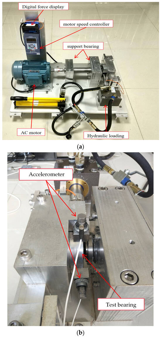
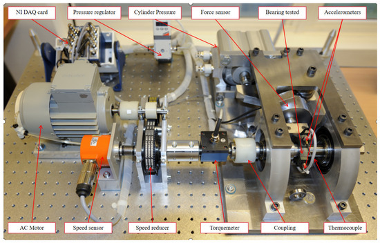
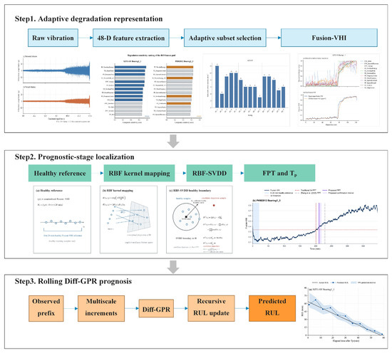
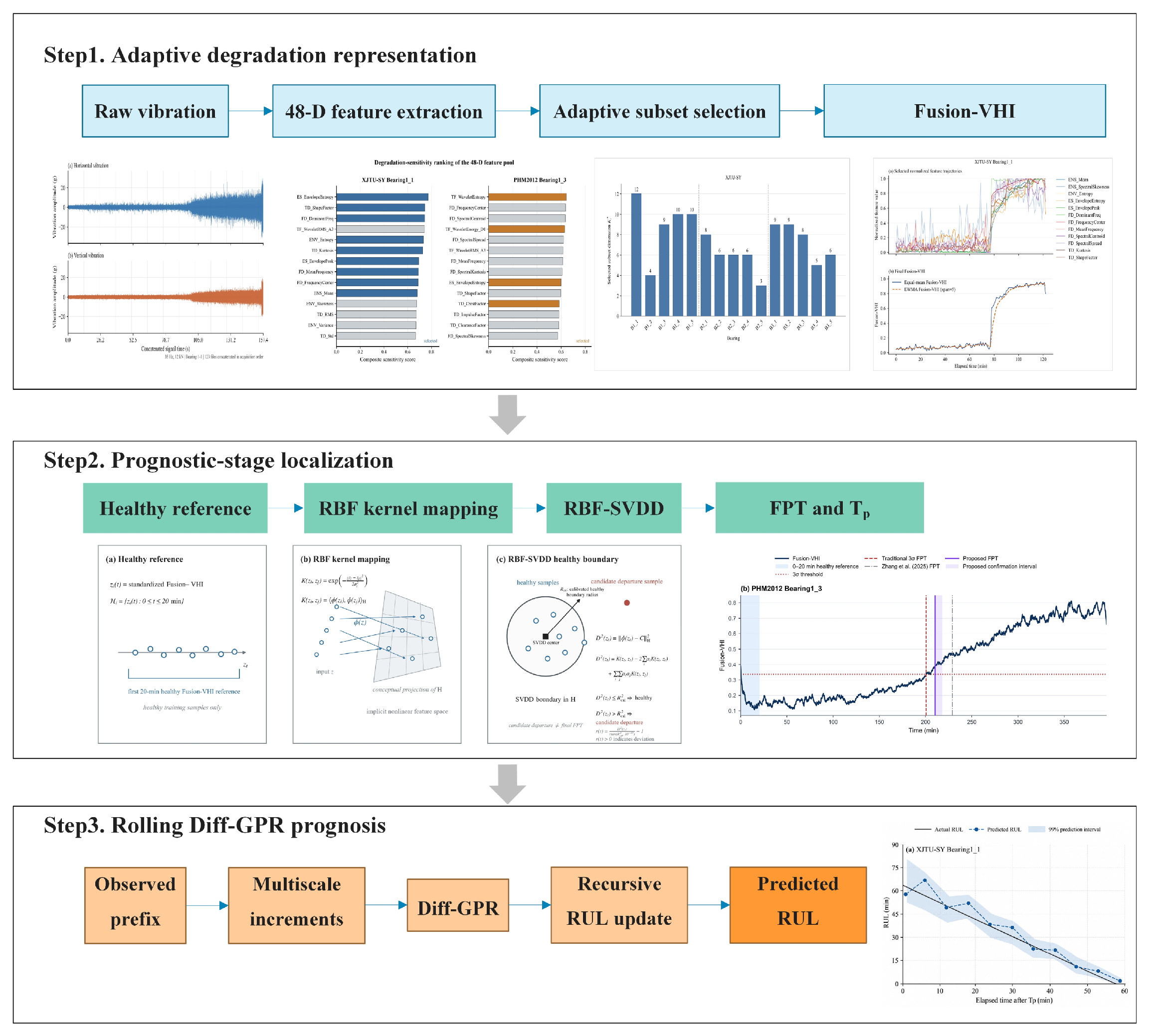
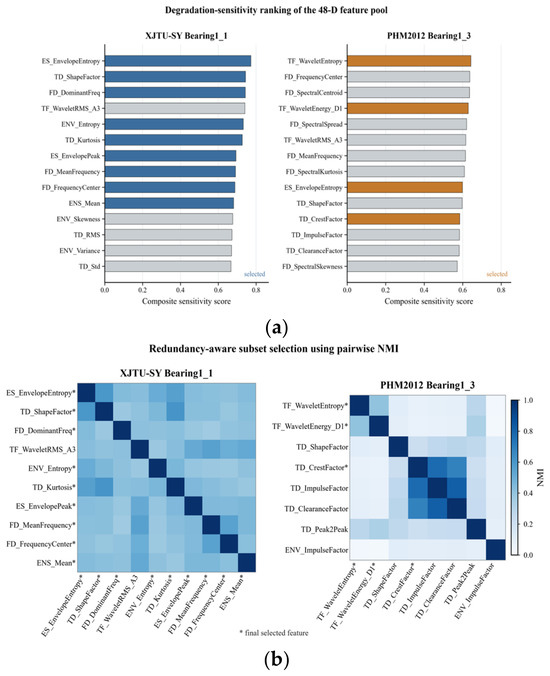
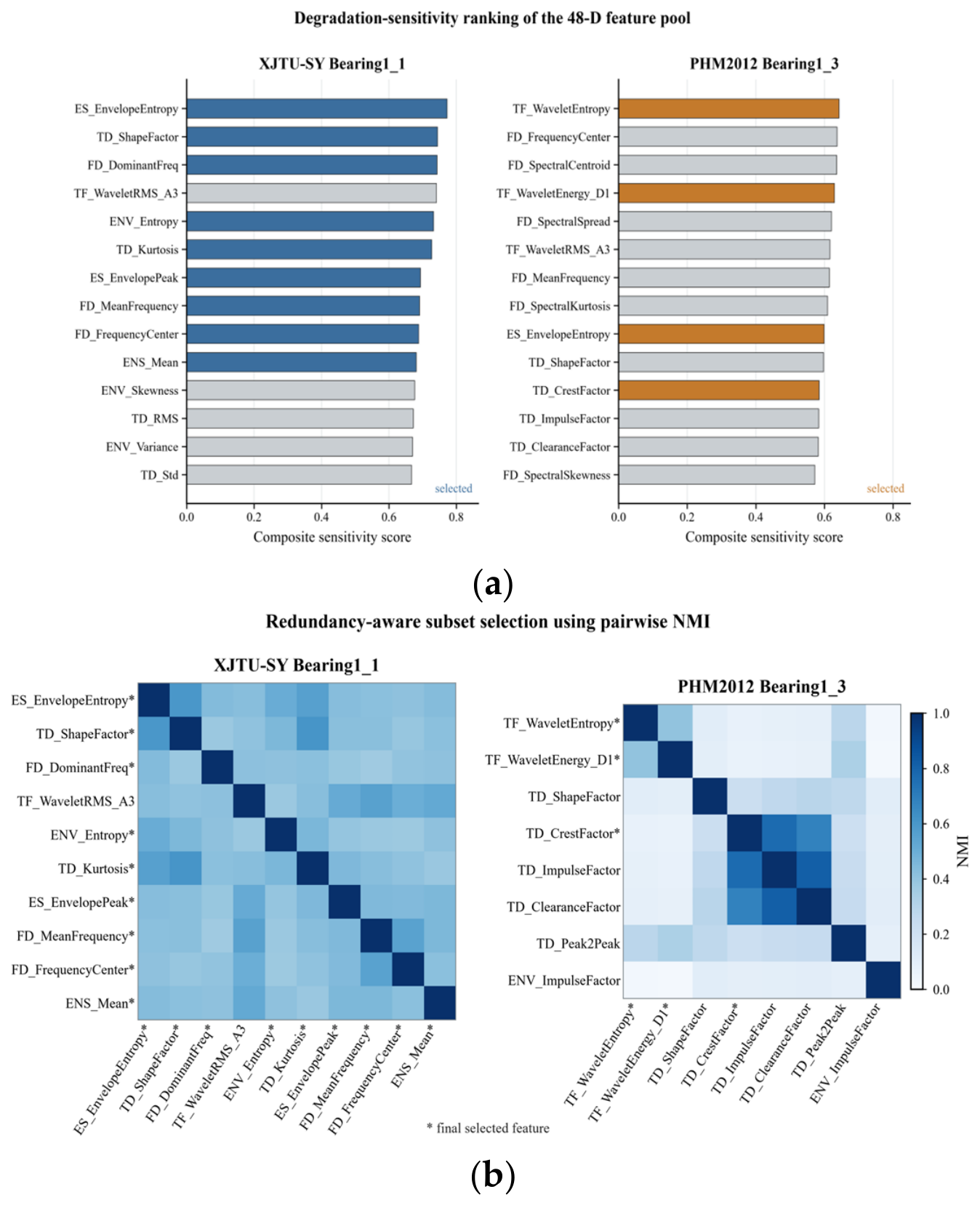
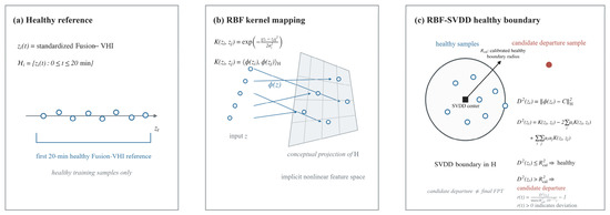
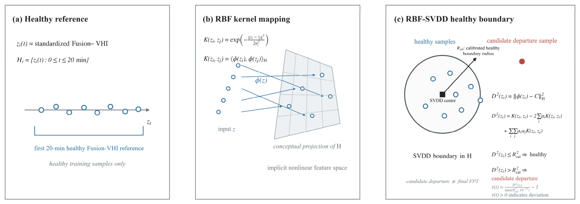
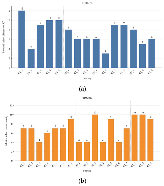
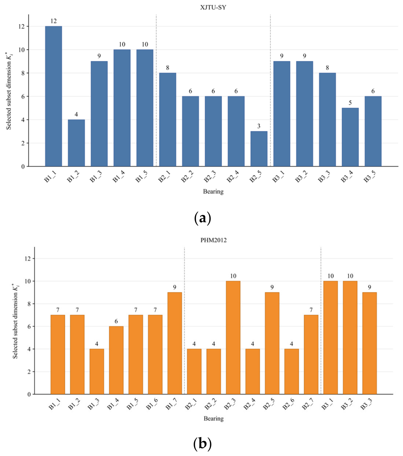
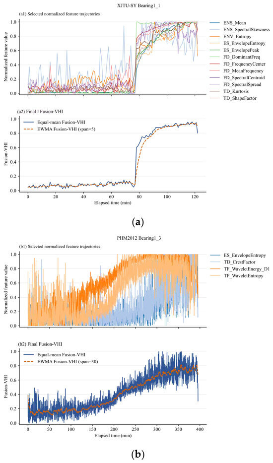
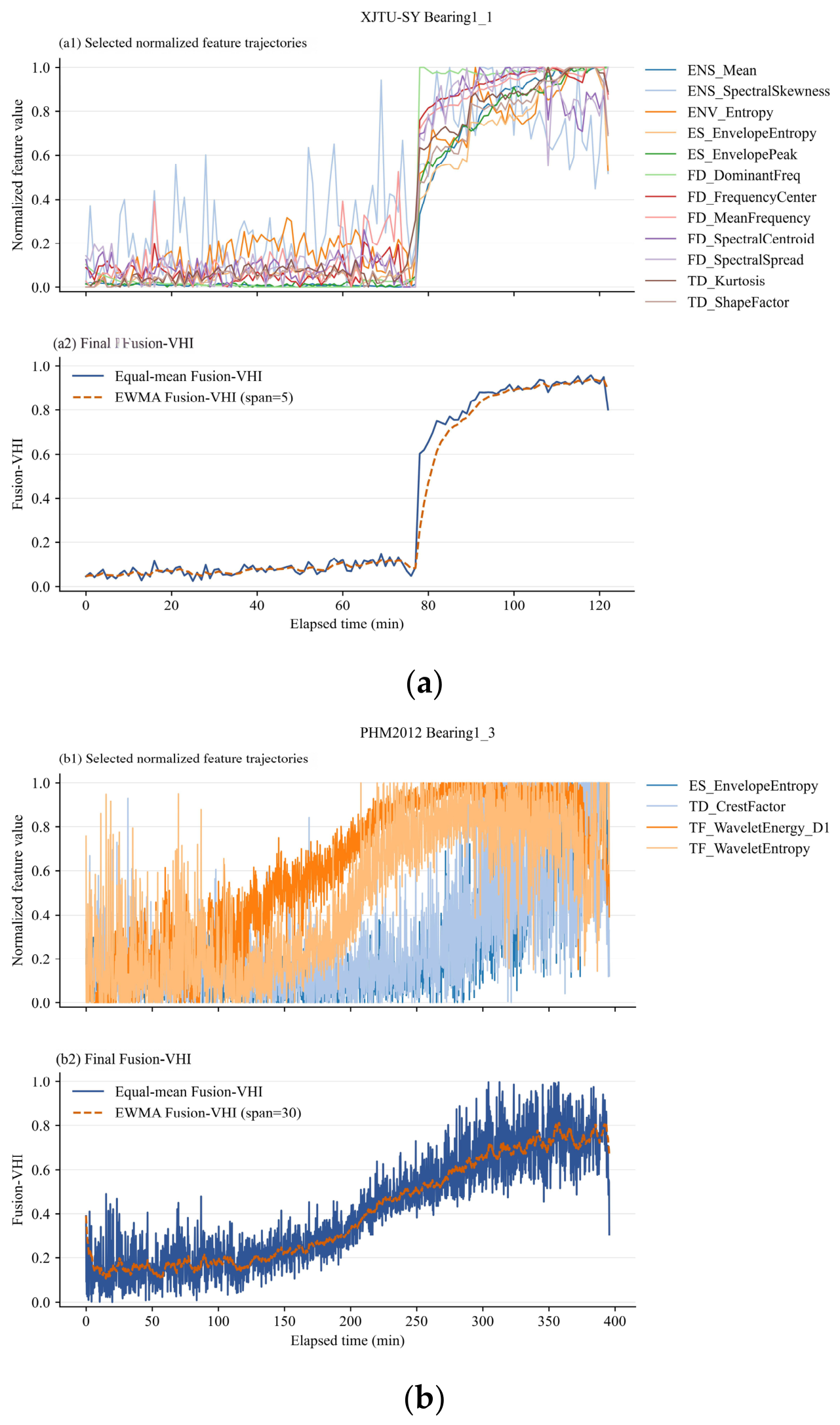
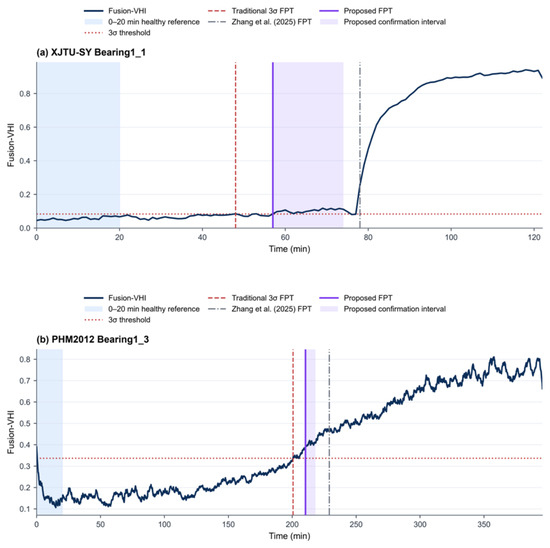
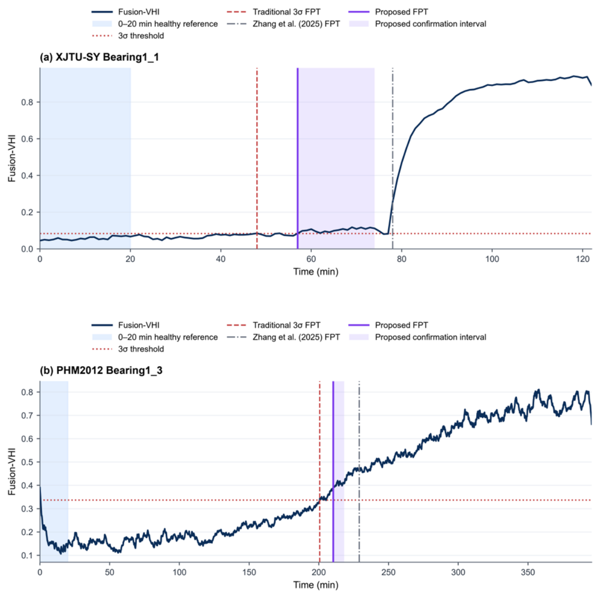
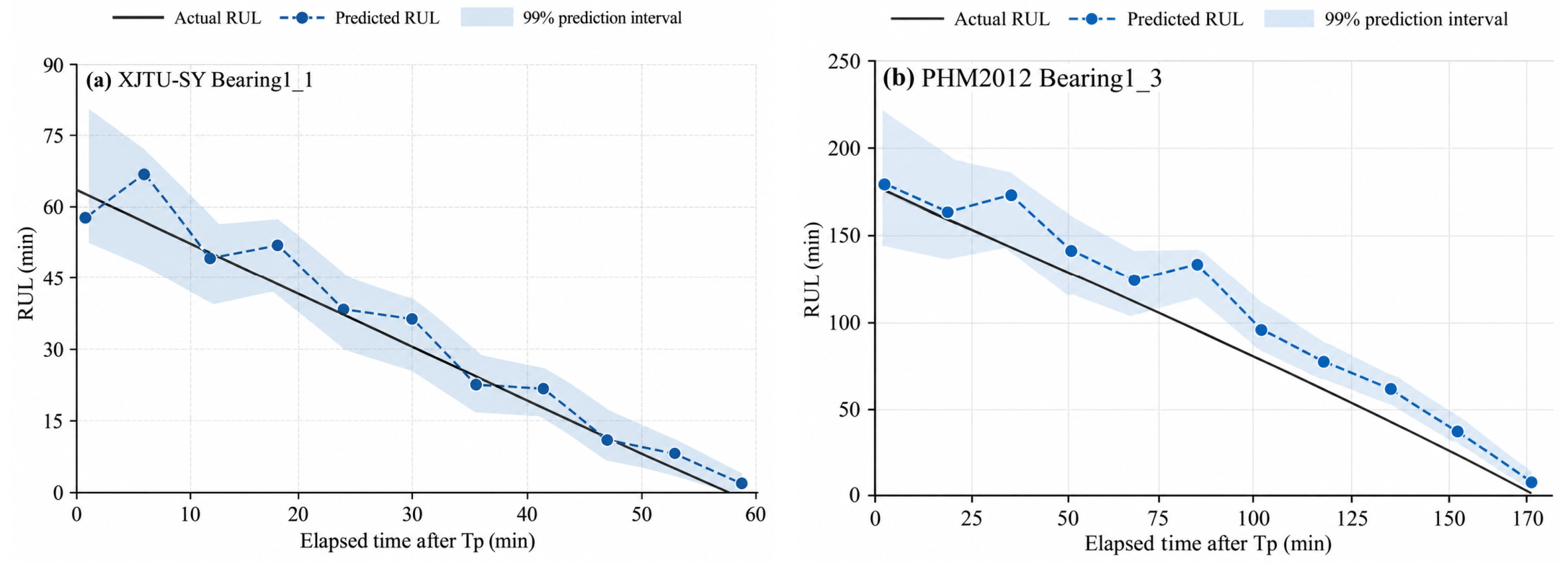
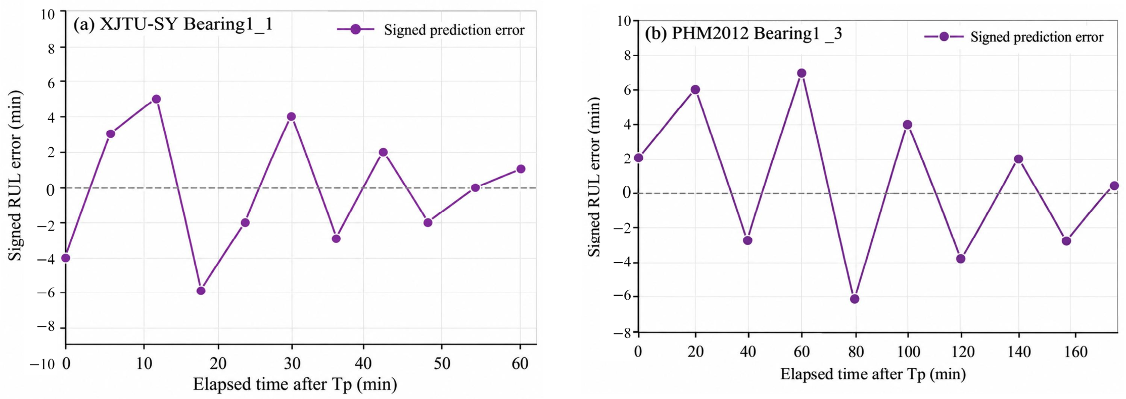

Disclaimer/Publisher’s Note: The statements, opinions and data contained in all publications are solely those of the individual author(s) and contributor(s) and not of MDPI and/or the editor(s). MDPI and/or the editor(s) disclaim responsibility for any injury to people or property resulting from any ideas, methods, instructions or products referred to in the content. |
© 2026 by the authors. Licensee MDPI, Basel, Switzerland. This article is an open access article distributed under the terms and conditions of the Creative Commons Attribution (CC BY) license.