


Abstract
Camouflage design for jungle environments has conventionally relied on the static optimization of color, texture, and edge features, presuming that the background remains visually stable. This presumption diverges from real conditions, in which wind continuously alters leaf orientation and vegetation texture, leaving a gap between static optimization and dynamic visual reality. To address this limitation, this study developed a systematic camouflage design process that integrates the Beaufort scale into a mimetic system for simulating vegetation sway. Dominant colors were extracted using the CIE L*a*b* color space and K-means clustering, and background maps were generated via Gaussian blur. Leaf textures from five plant species were arranged through seamless tiling and overlaid onto the backgrounds to form 15 camouflage samples. Validation employed a fuzzy logic questionnaire and eye-tracking measurements. Under the present experimental conditions, which used screen presentation under visible light, pattern A-13 performed best. Derived from the Terminalia mantaly leaf texture in the dark green variant, it achieved the most favorable balance between distinctiveness from the regional reference pattern and disruption of target–background segmentation, whereas C-15, the light green variant, consistently ranked last. The proposed process is reproducible and applicable to civilian equipment such as tents and backpacks.
1. Introduction
With the rapid advancement of military technology, the demand for concealment and camouflage on the battlefield has been increasing. Camouflage design, which plays an important role in reducing visual detectability in operational contexts, is fundamentally aimed at disrupting enemy detection and blending into the environment. Traditional camouflage, which mainly consists of irregular spots or stripes, is effective only at certain distances. Digital camouflage emphasizes the simulation of detail and three-dimensional textures, enabling more realistic blending into natural scenes and improving adaptability across diverse environments. Liu et al. [1] noted that during reconnaissance in warfare, blurred boundaries between targets and backgrounds create visual identification challenges. Li et al. [2] stated that traditional camouflage is inadequate against advanced reconnaissance technologies because these technologies enable multispectral and high-resolution detection, which can considerably improve target recognition. Furthermore, camouflage patterns used by forces operating in regional jungle environments may closely resemble those of neighboring countries; therefore, practical identification often depends on insignia or other uniform markings. This visual overlap can pose challenges for reliable unit recognition during field operations, highlighting the need for camouflage designs with greater perceptual distinctiveness.
Most camouflage research has focused on color optimization and pattern generation. Lin and Prasetyo [3] applied the particle swarm optimization algorithm to adjust the color parameters of camouflage such that its detectability was reduced in swamp environments. Goudarzi et al. [4] reproduced the reflective characteristics of green leaves through dye mixing and L*a*b* chromaticity analysis, thereby simulating the coloration of natural vegetation. However, most relevant studies have emphasized pattern correction and seldom integrated strategies combining visual cognition and background dynamics. Building on these color-focused approaches, a parallel body of work has examined the perceptual and biological foundations of camouflage mimicry.
Green [5], in Fundamentals and Applications of Color Engineering, noted that color can be described in terms of hue, saturation, and brightness, while the CIE L*a*b* model has been widely applied in image analysis. Ji et al. [6] further emphasized that the CIE L*a*b* space corresponds closely to human visual perception of color, and they proposed a polynomial regression model to improve the accuracy of the CIE L*a*b* model by reducing discrepancies between its values and human perceptual responses. Ohta [7] investigated the conversion relationship between the RGB and Munsell color systems, verifying the effect of such conversion on human visual perception. Lin et al. [8] used the response surface methodology on the L*, a*, and b* components in the CIE L*a*b* color space to enhance the effectiveness of military camouflage. They conducted K-means clustering within the CIE L*a*b* color space to improve the consistency between computer color rendering and human visual perception.
In terms of pattern generation, Hsiao and Tsai [9] developed a natural color transformation system that combines image segmentation with K-means to provide a more natural color scheme. Wan et al. [10] and Wei et al. [11] combined max pooling with K-means and the HSV model, respectively, to establish automated camouflage design processes, effectively reducing subjective design errors.
The theoretical framework of camouflage mimicry provides a crucial foundation for the pattern generation process. Cuthill et al. [12] indicated that the coloration of animal bodies serves multiple functions, such as social signaling, thermoregulation, and antipredation. Stevens and Merilaita [13] proposed camouflage strategies such as background matching, disruptive coloration, and shape concealment, highlighting the importance of integrating psychological, visual, and biological perspectives. The aforementioned studies support the use of natural leaf textures as the primary pattern source for camouflage, with these textures enhancing environmental blending and concealment.
In the field of visual cognition, Itti and Koch [14] proposed a visual attention mechanism through which humans cognitively separate a target from the background to quickly focus on information of interest. On the basis of this mechanism, they developed a camouflage pattern with low edge sharpness, allowing a camouflaged subject to be misperceived as being part of the background. Karthiga and Asuntha [15] employed the Canny algorithm to extract edge features and enhance contours of the camouflage motifs. Umeton et al. [16] proposed the concept of disruptive coloration, according to which high-contrast and discontinuous pattern elements are arranged at object boundaries to delay the detection and recognition of a target by observers. Troscianko et al. [17] quantified detectability by examining edge density, and Song et al. [18] developed a parallel algorithm to optimize large-scale edge processing. Daneshvar et al. [19] applied neural style transfer to generate blurred patterns. Moreover, Yang et al. [20] proposed a camouflage evaluation index based on comparisons of target and background color and texture features, which is used to assess camouflage performance. Hall [21] and Song [18] designed blurred backgrounds and visual click platforms. Barnett et al. [22] demonstrated that an increase in distance causes a decrease in spatial resolution (equivalent to visual blur), which results in high-contrast textures blending into the background and reduces recognizability. Finally, Barnett and Cuthill [23] obtained empirical evidence that a larger distance or blurring results in pattern fusion, making patterns more difficult to distinguish at a long range. Overall, the findings of the aforementioned studies confirm that blurring techniques can reduce visual salience and enhance camouflage effectiveness.
Although previous camouflage studies have improved color distribution, texture similarity, edge disruption, and visual salience, most have treated the background as visually stable. This assumption has been questioned in recent work on dynamic environments. Cuthill et al. [24] observed that most natural scenes contain dynamic elements, such as the motion of vegetation and the rapid variation in illumination, and that detection depends on the changing relationship between a target and its moving background. Brunyé et al. [25] examined how the speed of a target interacts with the properties of a pattern. They reported that local contrast and spatial frequency strongly influenced detection, and that movement alone was not sufficient to break a pattern that matched the background well. Van der Burg et al. [26] proposed an adaptive design that samples the background and accounts for the variation in viewing direction. Their design concealed moving targets more effectively than a method that simply displayed the exact background. These findings indicate that camouflage informed by a dynamic background offers a clear advantage over static optimization.
This limitation is especially relevant in jungle environments, where wind continuously alters leaf orientation, contour overlap, and vegetation texture. Such variation induced by wind may affect target detection by changing the visual relationship between the target and its background. However, existing digital and bionic camouflage designs rarely use wind speed or vegetation deformation as explicit design parameters. This study therefore introduces the Beaufort scale as a systematic basis for simulating the deformation of vegetation caused by wind and incorporating the characteristics of a dynamic background into camouflage pattern design.
Hashemi et al. [27] and Singleton [28] have highlighted the potential of using the Beaufort scale in the simulation of natural scenes. Niklas [29] explored how gravity and wind influence the evolution of terrestrial plants, applying the Euler–Greenhill formula and models of wind-induced drag forces from engineering mechanics to enhance the resistance of plants to toppling. However, existing digital camouflage designs do not sufficiently account for the influence of wind speed on plant morphology or the recognition differences under multispectral sensing, and a camouflage design method that integrates dynamic backgrounds with visual cognition models is lacking. Moreover, to the best of the researchers’ knowledge, no study has used the Beaufort scale in camouflage pattern design.
Understanding how observers detect camouflaged targets requires grounding in visual search theory, which informs the design of the evaluation framework employed in this study. Wolfe and Horowitz [30] proposed that five core factors, namely bottom-up salience, top-down feature guidance, scene structure and meaning, the previous history of search over timescales ranging from milliseconds to years, and the relative value of the targets and distractors guide attention in visual search. Henderson [31] proposed gaze control theory, which indicates that scene expectation and task orientation considerably affect fixation strategies. Denning [32] indicated that background matching can reduce camouflage visibility. Lin et al. [33] analyzed the light absorption characteristics of leaves in the short-wave infrared spectrum in terms of their spectral reflectance, providing insights into the design of camouflage materials and highlighting the necessity of spectral simulation in camouflage design.
A key challenge in the research on camouflage is to evaluate its effectiveness. Quantitative evaluation provides a crucial scientific basis for optimizing stealth strategies and objectively verifying camouflage performance. Moreover, eye-tracking instruments and fuzzy questionnaires can be employed to achieve dual-track validation. Brunyé et al. [34], Torrico et al. [35], Husic-Mehmedovic et al. [36], and Park et al. [37] have confirmed the value of eye tracking in analyzing visual salience and cognitive judgment. Analytical reliability can be enhanced through Pearson correlation analysis, as indicated by the quantitative validation methods of Gamino-Sánchez et al. [38] and the R Core Team [39].
In summary, although existing camouflage design research has focused on various aspects, such as color optimization and pattern generation, it has not integrated wind speed simulation, color computation, pattern generation, and visual validation into a single process. Therefore, the present study developed a camouflage design process that integrates the Beaufort scale-based mimetic system with background matching, using military garments as a case study to establish an expandable camouflage pattern evaluation platform. Dual-track validation using fuzzy logic questionnaire and eye-tracking measurements was conducted under screen-based visible-light conditions, with results indicating that dark green variants derived from Terminalia mantaly leaf textures showed the greatest perceptual distinctiveness from the regional reference pattern and the strongest visual disruption across both evaluation methods.
2. Materials and Methods
2.1. Overview of the Design Process
The proposed process consists of three main stages: main pattern construction, background pattern production, and dual-track validation, as illustrated in Figure 1.
Figure 1.
Flowchart of the research methodology. The dashed boxes indicate the two parallel construction processes described in Section 2.2 (Main Pattern Construction, left) and Section 2.3 (Background Pattern Construction, right), both of which converge in the camouflage clothing design and validation stages.
2.2. Main Pattern Construction
2.2.1. Leaf Image Collection and Species Selection
During main pattern construction, images of both the front and back sides of leaves from 10 common tree species in Taiwan were captured. Subsequently, a questionnaire survey was conducted on these species, with 145 valid responses collected. The results indicated that the top five species were Ficus microcarpa (81.4%), Alstonia scholaris (43.6%), Cinnamomum camphora (42.9%), Koelreuteria henryi (35.7%), and Terminalia mantaly (30.8%). Representative images of the selected leaf samples are shown in Figure 2. The captured images were converted into vector diagrams for use in subsequent feature recognition and analysis.
Figure 2.
Representative leaf vector images of the 5 plant species selected in this study.
A Canny edge extraction model was established and then integrated with the Beaufort scale to develop a Beaufort scale-based mimetic system. Edge extraction was then performed on the generated plant vector diagrams to obtain their shapes and features. The theoretical basis and specific implementation of these methods are described in the following sections.
2.2.2. Color Feature Extraction
In the RGB system, a color is described using a combination of red, green, and blue light intensities. To approximate human visual perception, the RGB color system is converted into the CIE XYZ system, which is subsequently modified into the CIE L*a*b* color space through nonlinear transformation. The matrix for conversion between the RGB and CIE XYZ systems as well as the white point are set according to the adopted color space (e.g., sRGB). The obtained XYZ coordinates are then converted into L*a*b* coordinates. The corresponding conversion formulas are expressed as follows:
where R, G, and B represent the intensities of red, green, and blue light, respectively, in the RGB color space; X, Y, and Z are the color coordinates in the CIE 1931 XYZ color space; and , , and are the CIE XYZ coordinates of the reference white point. Under the commonly used D65 light source, = 95.047, = 100.000, and = 108.883. The term denotes lightness, which indicates the brightness of a color, and ranges from 0 (black) to 100 (white); is the color on the green-red axis, where a positive value indicates red, and a negative value indicates green; and is the color on the blue-yellow axis, where a positive value indicates yellow, and a negative value indicates blue. Finally, , , and are the normalized XYZ components obtained after nonlinear cube-root transformation is conducted. These components are used to approximate the nonlinear perceptual characteristics of human vision with respect to brightness and color changes.
Following the conversion of image data into the CIE L*a*b* color space, k-means clustering was applied to extract representative colors from the collected jungle environment images. The k-means algorithm is a commonly used unsupervised clustering method. Its goal is to partition a dataset into k clusters and assign data points to these clusters on the basis of distance.
The algorithm minimizes the within-cluster sum of squares (SSE) in CIE L*a*b* space, as defined in Equation (5). The algorithm iteratively alternates between assignment and update steps until convergence. The main steps are:
- Initialize: Randomly select k data points as initial centroids {μ1(0), …, μₖ(0)}.
- Assignment: Assign each data point to the nearest centroid (using Euclidean distance), as formalized in Equation (6).
- Update: Recalculate each cluster centroid as the mean of assigned points, as given in Equation (7).
- Convergence: Steps 2–3 are repeated until either the relative reduction in the objective falls below a predefined tolerance [Equation (8)] or the cluster assignments remain unchanged between successive iterations [Equation (9)]. The maximum number of iterations was set to 300 as a safeguard against non-convergence.where is the th point in CIE L*a*b* (D65); cᵢ ∈ {1, …, k} is its hard assignment; is the assigned centroid; {μ1, …, μₖ} are the k centroids; denotes the Euclidean norm; is the within-cluster sum of squares (SSE).
The assignment rule and the centroid update are given by
where each is assigned to the nearest centroid in L*a*b*.
where is the centroid (arithmetic mean) of cluster ; is its size.
where is the objective at iteration ; ε > 0 is a small tolerance; the second condition indicates no change in assignments.
The alternating assignment-update scheme monotonically decreases the objective J and, in finitely many steps, converges to a local minimum. Geometrically, the centroids induce a Voronoi tessellation in the feature space. The method implicitly assumes roughly spherical clusters with comparable variance and uses the arithmetic mean as the centroidal representative; owing to the quadratic loss, it is sensitive to outliers. Furthermore, all distances are computed in CIE L*a*b* using the Euclidean metric. Because L*a*b* is approximately perceptually uniform under D65, these distances align more closely with visual color differences than RGB; to enhance perceptual robustness, this study additionally conducted a sensitivity check using the CIE DE2000 color-difference metric. The k-means formulation defined in Equations (5)–(9) was applied at two stages. In main pattern construction, it extracted representative colors from leaf images. In background pattern production, it identified dominant colors from jungle background photographs (Section 2.3.1). Using the same formulation at both stages maintained methodological consistency across the two pattern layers.
2.2.3. Edge Extraction (Canny Method)
Canny edge detection is a technique in which edges are detected using image gradients and a dual-threshold hysteresis procedure. This technique is performed in the following sequence: Gaussian smoothing for noise reduction, gradient computation, nonmaximum suppression, and dual thresholding and edge tracking by hysteresis. The objectives of the technique are (1) to maximize the output signal-to-noise ratio (SNR) while reducing missed and false detections, (2) to accurately detect edge locations, and (3) to generate a single response for each edge. Canny edge detection involves the following steps:
- Compute the edge response and SNR by using the following equation:where f(x) represents the impulse response function of the edge detector, G(x) is the edge model signal, and dx denotes a small change in variable x. Equation (10) indicates that the areas corresponding to G(−x) f(x) are summed within the interval [−W, W]. If the integration is performed with respect to y, the differential is written as dy; for two-dimensional integration, it is written as dx, dy, or dA, indicating integration over a planar region.
- Calculate the localization accuracy by using the following Equation (11):where x0 is the displacement of the extreme position caused by noise; is the localization error; is the mean square value of white noise per unit length; is the first derivative, which is used for estimating the spacing of extreme values; is the derivative of the edge signal; and Localization denotes the localization accuracy of edge detection.
- Eliminate multiple responses. To eliminate multiple responses along an edge, nonmaximum suppression is applied. At each pixel, the gradient direction is computed and quantized into one of four principal orientations. The gradient magnitude of the current pixel is then compared with its two neighbors along this direction. If the current pixel is not a local maximum, its value is suppressed to zero. This procedure ensures that only one-pixel-wide edge responses are preserved. According to Rice’s theorem, the expected distance between neighboring response peaks under noise can be expressed as follows:where is the expected distance between neighboring response peaks under noise; is the second derivative, which is used for estimating the spacing of extreme values; w is the filter width; and k is the ratio between the spacing of extreme values and the filter width.
- Use the following equation to efficiently obtain an approximation of the optimal filter on the basis of the first derivative of the Gaussian function:where is the Gaussian standard deviation. This approximation achieves approximately 90% of the theoretical performance, has high computational efficiency, and is commonly implemented in image processing systems.
In this study, the accuracy of outer contour extraction and the degree of noise suppression were adopted as the primary criteria for parameter optimization. Experimental results identify a Gaussian kernel size of 11 (corresponding to σ ≈ 2.15) combined with a gray threshold of 244 as the optimal configuration. This setting yielded the most complete and continuous leaf outer contours, with smooth boundary lines, no significant residual noise, and the most satisfactory background removal results. Accordingly, this parameter configuration is identified as the optimal setting in the present study. By comparison, a kernel size of 3 preserved richer vein detail but introduced substantial high-frequency noise. The resulting contour lines were fragmented and unsuitable for direct use in subsequent pattern generation. A kernel size of 6 represented an intermediate case, offering acceptable contour clarity but with residual noise points that compromised overall contour integrity. Based on the foregoing comparative analysis, this study concludes that a larger Gaussian kernel size combined with a higher threshold value should be prioritized when plant outer contours serve as source material for subsequent pattern design. This parameter choice ensures sufficient smoothness and completeness of the extracted contours, thereby reducing post-processing burden and enhancing the overall efficiency of the design workflow.
2.2.4. Beaufort Scale-Based Deformation Model
Within the proposed Beaufort scale-based mimetic system, the deformation model served as the core computational module for translating wind intensity into species-specific leaf deformation. This model converted Beaufort scale levels into wind speeds, estimated aerodynamic loading on leaf blades, calculated tip deflection using beam-theory assumptions, and generated the corresponding deformation angles for subsequent pattern construction.
The Beaufort scale is a thirteen-level classification system (0–12) used to describe wind force intensity, ranging from calm conditions (B0) to hurricane-force winds (B12). The B6–B9 range was selected for three reasons. First, wind levels below B6 generally produce only minor leaf rustling or branch oscillation, resulting in deformation that is visually close to static conditions and therefore unsuitable for testing wind-induced camouflage variation. Second, wind levels above B9 correspond to storm-force conditions, under which sustained outdoor field activity becomes operationally impractical. Third, B6–B9 represents a realistic range of wind conditions in subtropical mountainous regions and exposed ridges [40], including stronger winds associated with typhoon peripheries and orographic acceleration [41].
Taken together, the B6–B9 range constitutes a gradient of four levels that is perceptually meaningful (with sufficient magnitude of deformation to differentiate it from static conditions), operationally relevant (within the range of feasible field activity), and climatically representative (matching the dominant wind regime of the study region). This range enables a systematic comparison of vegetation deformation states across a continuous and practically grounded gradient, while B9 specifically establishes the upper boundary of the deformation envelope, allowing the camouflage design to be tested under realistic extreme conditions to the limits of stress. Table 1 summarizes the ranges of wind speed and the corresponding Beaufort classifications for B6–B9.
where v is the wind speed (m/s), and B is the Beaufort scale level. This equation originates from the original Beaufort scale definition and has been adopted as the standard WMO conversion formula [42].
Table 1.
Beaufort Scale (B6–B9 range adopted in this study).
The aerodynamic drag force per unit length of leaf, (N/m), is calculated using the quasi-static flat-plate drag formulation from fluid mechanics:
where is the air density, is the drag coefficient, w is the leaf blade width, and v is the wind speed. Under standard atmospheric conditions (15 °C, 101.325 kPa), the air density was assumed to be 1.225 kg/m3. The drag coefficient was set to 1.28, corresponding to a flat plate positioned normal to the airflow. The leaf blade width, w, was determined from species-specific measurements, and the wind speed, v, was obtained from Equation (14) for each Beaufort wind level. Therefore, denotes the distributed aerodynamic drag force along the leaf length, expressed in N/m.
Applying Euler–Bernoulli beam theory to a cantilever under a uniformly distributed load (UDL), the maximum tip deflection is
where L is the effective leaf blade length (m), E is the Young’s modulus of the leaf blade material (Pa), and I is the second moment of area of the leaf cross-section (). The parameter E represents the elastic stiffness of the leaf blade material. According to Sun et al. [43], the Young’s modulus of leaf tissues varies markedly with tissue type, structural organization, hydration state, and loading direction. Therefore, in this study, E was defined on the basis of the species-specific mechanical properties of the examined leaf blade.
The second moment of area, I, was approximated by assuming an elliptical cross-section of the leaf blade, which can be expressed as
where t denotes the midrib thickness (m) and w denotes the leaf blade width (m). Therefore, represents the maximum displacement at the leaf tip under wind-induced loading.
The leaf-tip deflection angle θ (degrees) is derived from
and leaf length L:
The computed deflection angle θ serves as the direct input parameter for the image deformation algorithm, where it governs the rotation angle in the affine transformation applied to each species-specific leaf texture image. A separate θ value is computed for each species at each of the four Beaufort levels (B6–B9), yielding a 4 × 5 matrix of deformation states (Table 2). Thus, the deformation workflow proceeded sequentially from Beaufort level selection to wind-speed conversion, aerodynamic loading estimation, elastic tip deflection calculation, angular transformation, and finally affine deformation of the leaf texture.
Table 2.
Estimated Deflection Angles (°) of Each Plant Species under B6–B9 Condition.
Finally, a graphical user interface was constructed for object simulation, and wind dynamics simulation was executed according to the Beaufort scale formula in Equation (14). The system simulation results are shown in Figure 3.
Figure 3.
Simulation results of the developed Beaufort scale-based mimetic system.
Figure 4a–d show the leaf deformation process under four Beaufort scale levels (B6–B9). For the representative leaf used in this demonstration, the estimated deflection angles were 8.7721°, 13.7683°, 20.0910°, and 27.5102°, respectively.
Figure 4.
(a) Deformation process under B6 levels, (b) deformation process under B7 levels, (c) deformation process under B8 levels and (d) deformation process under B9 levels.
The following effects were achieved by placing leaves with varying degrees of deformation into a nine-grid layout and aligning them with the surrounding grid lines:
- Seamless connection and extension: The main pattern in the central grid extended through the grid lines to the surrounding cells, forming a continuous natural transition in all four directions, ensuring that the pattern could be infinitely tiled without appearing abrupt.
- Visual dynamic illusion: The intersection points of the rule of thirds became the visual focal points. When different wind forces (B6, B7, B8, and B9) caused diverse deformations and arrangements of the leaves, observers perceived an optical illusion as if the image was flowing or swaying in the wind.
- Sense of layering and balance: The structure of the rule of thirds ensured a reasonable distribution of plant motifs of different sizes and orientations across the image, with overall balance and visual depth being maintained. After the aforementioned steps were completed, the main pattern was produced. Multiple main patterns were generated for different plants (Figure 5).Figure 5. Main patterns generated for the five selected plant species: (a) Ficus microcarpa; (b) Alstonia scholaris; (c) Cinnamomum camphora; (d) Koelreuteria henryi; and (e) Terminalia mantaly. Within each subfigure, the solid dark green leaf represents the B9 deformation level, while the dark green, medium green, and light green outlined leaves represent the B8, B7, and B6 levels, respectively.
After the Beaufort scale-based deformation process was completed, the deformed leaf motifs were arranged using a four-directional repeat tiling method combined with a nine-grid layout. In this procedure, pattern elements were continuously connected upward, downward, leftward, and rightward to ensure seamless edge transitions and enable infinite tiling for large-area fabric applications. The nine-grid layout, shown in Figure 6a–c, followed the rule-of-thirds composition principle by dividing the image into three equal sections both vertically and horizontally. This arrangement guided the distribution of visual focus along the grid intersections and facilitated the natural extension of leaf motifs across grid boundaries, thereby producing continuous camouflage textures with seamless tiling effects.
Figure 6.
(a) Nine-grid layout adhering to the rule-of-thirds composition principle, with the four Beaufort scale levels (B6–B9) assigned to designated grid positions; (b) leaf line drawings obtained through the four-direction repeat tiling method; and (c) main pattern obtained after color filling and multilayer superposition. Because only three representative colors were available for four Beaufort levels, B9 is rendered as a solid dark green fill, while B8, B7, and B6 are rendered as unfilled outlines in dark green, medium green, and light green, respectively. Leaf motifs extending beyond the panel boundaries in (b,c) reflect the four-direction repeat tiling design, which allows the pattern to connect seamlessly when tiled across a larger area.
To validate the arrangement logic embedded in the dynamic mimetic model, a large-scale frequency analysis was conducted on 3,843,356 texture layout images systematically collected from publicly available design databases, fabric pattern archives, and camouflage reference repositories. Prior to classification, all images were cropped to a standardized 3 × 3 aspect-ratio texture unit retaining the central contiguous grid block of each image, followed by data cleaning, category labeling, and size normalization as preprocessing steps.
A modified AlexNet architecture [44,45,46,47] was applied to categorize each image into one of five arrangement types: regular grid, diagonal, staggered, radial, and organic scatter. The original AlexNet backbone of five convolutional layers and three fully connected layers with ReLU activation, overlapping max pooling, and Dropout regularization (p = 0.5) was retained as the structural foundation, with three task-specific adaptations introduced to suit the present classification task. The Softmax output layer was reconfigured from 1000 classes to 5 classes corresponding to the five arrangement categories. All input images were cropped to a 3 × 3 aspect-ratio texture unit, aligning the spatial scale of the CNN receptive field with the structural rhythm of the patterns [46]. Residual learning principles were additionally incorporated to ensure stable gradient flow during training on the large-scale corpus. The model was trained on an MSI GeForce RTX 3080 GPU (10 GB GDDR6X VRAM; 8704 CUDA cores) using categorical cross-entropy loss, achieving an overall classification accuracy of 92.3% across the five arrangement categories [47].
In addition, the complete training configuration and performance metrics of the AlexNet classifier are provided in Appendix A, Table A1.
The analysis revealed that staggered (brick-bond) and diagonal offset arrangements collectively accounted for the highest proportion of usage across the corpus, followed by regular orthogonal grid and radial scatter patterns. Accordingly, the four Beaufort-level motifs (B6–B9) were assigned to positions within the nine-grid layout following a diagonal offset rule, ensuring that the proposed design inherits the statistically dominant arrangement pattern observed in real-world practice.
2.3. Background Pattern Construction
2.3.1. Color Clustering and Frequency Analysis
Background patterns were generated to achieve a blended effect with natural jungle environments. In background pattern production, image synthesis was conducted using the results of the k-means method and Gaussian blur. The k-means method was used for color clustering, and the resulting cluster counts were [330, 299, 224, 207, 180]. These values are reported in the CIE L*a*b coordinate system normalized to the range 0–1, and correspond to the five centroid locations {μ1, …, μ5} in CIE L*a*b space. On this basis, five basic colors were identified for constructing color samples for the natural database.
Prior to the color frequency analysis, the number of clusters k was determined through a preliminary perceptual experiment rather than by purely algorithmic criteria, with the aim of aligning the clustering parameter with the perceptual conditions under which camouflage garments are typically observed. A questionnaire was administered to 94 members of the general public, each asked to perform a rapid visual scan of a garment printed with a landscape image from a viewing distance of 30 m and a scanning duration of 2 s, and to report the colors they were able to identify. Responses ranged from three to five colors across all respondents, with five representing the upper bound of perceptual color resolution under brief distant observation. Accordingly, k = 5 was adopted as the clustering parameter, ensuring that the number of representative colors extracted by the algorithm corresponds to the perceptual ceiling identified in this preliminary experiment.
Color frequency analysis was then conducted on 451 images of forested areas in Taiwan, with the color values modeled using a normal distribution. After distribution thresholds were set, 248 unsuitable images were eliminated (Figure 7). These colors mostly originated from images containing non-natural elements such as artificial clutter, trains, and other vehicles, as well as irrelevant natural elements such as the sky. To assess perceptual robustness, 5000 pixels were randomly drawn from the 451 jungle background images, and cluster assignments were recomputed under the CIE DE2000 metric and compared against the baseline employing Euclidean distance in CIE L*a*b* space. Agreement between the two metrics reached 91.0%, indicating that cluster membership remains substantially invariant to the choice of perceptual distance metric within the L*a*b* color space. Finally, three representative colors (CIE L*a*b*) were selected as the camouflage base: [L* 62.54, a* −30.17, b* 38.96], [L* 45.45, a* −29.51, b* 38.93], and [L* 27.24, a* −25.00, b* 31.45]. The database was rescreened to retain images with the highest proportions of these three colors. Moreover, the three colors were applied to the vector diagrams of the leaves of the five plant species for color matching applications.
Figure 7.
Color distribution in the captured images of forested areas in Taiwan.
2.3.2. Gaussian Blur and Low-Frequency Background
Gaussian blur is a commonly used image processing technique that reduces the high-frequency noise in an image and enhances the smoothness of edge transitions. This technique can be considered to be equivalent to performing a weighted average on each pixel value in an image. The weights are determined according to the Gaussian distribution function, with pixels closer to the center having higher weights, as formalized in Equation (19). For example, when a 3 × 3 Gaussian convolution kernel is used, the weights of the center pixel and surrounding pixels are 2 and 1, respectively. After normalization, the weight of the center pixel is converted to 0.11185. Figure 8a illustrates the distance with its center at (0,0), prior to normalization. Substituting into Equation (19) transforms the central value from 0 to 1, with the values at distances of 2 and 1 becoming 0.11074 and 0.11130, respectively. Figure 8b presents the normalized kernel = 8.9402492518) with the central element highlighted in dark gray. The weighting process reduces excessive image details and noise, and the resultant image appears smoothed, showing blurred edges and softening effects (Figure 8c,d).
Figure 8.
(a) Distance grid (r²) of a 3 × 3 Gaussian kernel, with the center pixel highlighted in magenta; (b) normalized Gaussian kernel weights, with the center weight highlighted in dark gray; (c) original jungle background image; and (d) resulting image after Gaussian blur.
In Equation (18), denotes the standard deviation of the Gaussian function, which controls the degree of blurring; x and y denote the horizontal and vertical offsets of a pixel from the kernel center; and is Euler’s number (the base of the natural logarithm ≈ 2.71828).
Subsequently, Gaussian blur and an overlay weighted by representative colors were performed. The selection of the Gaussian standard deviation σ governs the trade-off between two competing requirements in background pattern generation: sufficient smoothing of fine texture detail to simulate the soft, defocused appearance of distant jungle scenes, and adequate preservation of broad color gradation to retain the natural tonal structure of the original environment. To determine the optimal value, a comparative evaluation was conducted across five σ levels (σ = 2, 5, 10, 15, 20) applied to the same set of jungle background images, with the 21 × 21 kernel size held constant and reflect padding applied at image boundaries.
The comparison was evaluated against three criteria. The first, residual texture detail, was quantified by the standard deviation of pixel intensities in the blurred image, where lower values indicate stronger smoothing. The second, color tone preservation, was measured by the CIE DE2000 color difference between the mean color of the blurred image and the mean color of the three representative CIE L*a*b* centroids; lower CIE DE2000 values indicate better convergence toward the target representative colors. The third, perceptual depth-of-field quality, was determined through an expert panel assessment of composite samples generated under each σ value.
For the assessment of perceptual depth-of-field quality, the blurred background generated under each σ value was composited with the vectorized leaf textures derived in Section 2.2 to produce five representative camouflage samples exhibiting varying degrees of depth-of-field differentiation. These samples were independently evaluated by a panel of 22 visual design experts, each with a minimum of five years of professional experience in graphic, textile, or visual communication design. Each expert reviewed all five samples under a controlled lighting environment and selected the configuration that best achieved the perceptual depth-of-field effect characteristic of distant jungle viewing.
Results across the three criteria converged on σ = 10 as the optimal parameter. As illustrated in Figure 9, at σ = 2 and σ = 5 (Figure 9a,b), fine texture details such as leaf veins and small branches remained visible, producing insufficient blur to simulate distant jungle viewing. At σ = 15 and σ = 20 (Figure 9d,e), although smoothing was more aggressive, the resulting image exhibited excessive uniformity and lost the subtle tonal gradations of the natural background, producing a flat appearance inconsistent with realistic jungle environments. The expert panel likewise selected σ = 10 (Figure 9c) as the configuration best representing natural jungle depth-of-field perception. Furthermore, at σ = 10, the blurred image color converged most closely toward the three representative CIE L*a*b* centroids identified in Section 2.3.1, supporting subsequent representative-color-weighted overlay. Accordingly, σ = 10 was adopted as the optimal parameter setting throughout this study. The final low-frequency backgrounds produced under σ = 10 for the three color variants are presented in Figure 10a,c.
Figure 9.
Comparison of composite camouflage samples generated under different Gaussian σ values: (a) σ = 2; (b) σ = 5; (c) σ = 10; (d) σ = 15; and (e) σ = 20. The leaf textures were colored using the three representative colors derived from clustering and frequency analysis of forest background images in Taiwan; σ = 10 was identified as the optimal parameter.
Figure 10.
Low-frequency background synthesis and representative-color steering. (a) Dark green variant; (b) neutral green variant; (c) light green variant. Gaussian blur: σ = 10, 21 × 21, reflect padding. Recoloring: Softmax weights over CIE DE2000 to the three CIE L*a*b* representatives.
2.4. Design of Camouflage Uniforms
After the main and background patterns were generated, the developed mimetic model was used to integrate these patterns. The main patterns, which were based on the morphological features of plant leaves, conveyed natural forms. By contrast, the background patterns, which were processed through k-means color clustering and Gaussian blur, simulated the color transitions and gradations of natural environments. To achieve large-area seamless tiling of the patterns, the four-direction repeat tiling method was applied, ensuring seamless connection between the main and background patterns, thereby producing a camouflage pattern with overall visual consistency.
The mimetic system generated 5 sets of main patterns, each of which was combined with three background patterns to produce a total of 15 camouflage samples. The samples were coded according to color tone, with the dark green, neutral green, and light green samples coded as A, B, and C, respectively; the sample numbers are shown in Figure 11. Color codes: A-series (dark green, L* = 27.24), B-series (neutral green, L* = 45.45) and C-series (light green, L* = 62.54), respectively. The samples were then employed to design prototype military camouflage uniforms, with pattern continuity and visual balance adjusted at different parts of the uniforms, such as the cuffs, shoulders, and trouser legs, thereby enhancing concealment and overall esthetics.
Figure 11.
Application of the designed camouflage patterns to military uniforms.
Finally, the Marvelous Designer 11 (CLO Virtual Fashion, Gangnam-gu, Seoul, Republic of Korea) clothing design software program was used to conduct three-dimensional virtual simulations, with the designed camouflage samples applied to military uniform models (Figure 11). The sample coding was defined as follows: A-1, B-2, and C-3 represented F. microcarpa leaf texture; A-4, B-5, and C-6 represented A. scholaris leaf texture; A-7, B-8, and C-9 represented C. camphora leaf texture; A-10, B-11, and C-12 represented K. henryi leaf texture; and A-13, B-14, and C-15 represented T. mantaly leaf texture. The completed designs were also experimentally placed into jungle and hill scenes for camouflage effect simulation and visual testing (Figure 12).
Figure 12.
Simulated camouflage performance in (a) a jungle scene and (b) a hill scene. The human figures were generated as synthetic 3D models using KeyShot 10 (KeyShot, Inc., Tustin, CA, USA) and composited onto real background imagery using Adobe Photoshop 2020 (Adobe Inc., San Jose, CA, USA). All human figures depicted are computer generated and do not represent real individuals.
2.5. Validation
2.5.1. Fuzzy Logic Questionnaire
A questionnaire survey was administered, yielding a total of 145 valid responses. Respondents were recruited through the Facebook community groups of university departmental student associations. All reported normal or corrected vision, with no color blindness or color vision deficiency, and no ocular disease. Respondents with professional military training, camouflage design experience, or formal visual search training were excluded, so that the sample represented untrained observers. This was done to reduce bias caused by prior familiarity with military uniforms or camouflage recognition. The survey employed a pairwise comparison approach, in which respondents assessed two camouflage images simultaneously using a fuzzy rating scale comprising the following options: 0 = extremely dissimilar, 0.25 = slightly dissimilar, 0.5 = neutral, 0.75 = slightly similar, and 1 = extremely similar. Respondents first rated the similarity among the 15 camouflage samples developed in this study. This step examined the perceptual differences among the leaf texture patterns and established a basis for assessing the distinctiveness of each design. Using the simulated scenario images presented in Figure 12a,b, respondents further applied the same rating scale to assess the visual similarity between each of the 15 camouflage samples and a reference sample representing a commonly used regional camouflage pattern, designated as D-16 and illustrated in Figure 13. In this study, D-16 was not only used as a regional reference pattern but also treated as a representative static-pattern camouflage sample. It therefore provided a comparative baseline for distinguishing conventional static camouflage from the proposed Beaufort scale-based dynamic mimetic camouflage designs. The purpose of this stage was to determine whether the camouflage patterns developed in the present study are perceptually distinguishable from existing regional and static-pattern camouflage designs, thereby supporting design distinctiveness and reducing the likelihood of visual confusion in field applications.
Figure 13.
Reference camouflage sample D-16, representing a commonly used regional camouflage pattern adopted as the visual comparison baseline in this study.
2.5.2. Eye-Tracking Experiment
The required sample size for the eye-tracking experiment was determined a priori using G*Power 3.1 (Heinrich-Heine-Universität Düsseldorf, Düsseldorf, Germany) [48]. On the basis of a target medium effect size (Cohen’s f = 0.25), a significance level of α = 0.05, and a desired statistical power of 1 − β = 0.80, the minimum required sample size for a one-way repeated-measures ANOVA with 16 conditions was estimated to be 42 participants. The enrolled sample of 52 participants therefore exceeded this threshold, providing adequate power for the planned comparisons.
To investigate the camouflage effectiveness of the designed camouflage samples, 52 participants (29 men and 23 women, with 86.9% aged 21–40 years) were invited to participate in an eye-tracking experiment (Figure 14). Participants were recruited through the same channel and met the same eligibility criteria as the questionnaire respondents. Eligibility required a visual acuity of 0.8–1.0 in decimal notation, equivalent to approximately 20/25 to 20/20 (6/7.5 to 6/6). Because the experiment measured pupil diameter, participants were required to have no pupillary abnormality, and the use of decorative contact lenses that obscure the pupil boundary was not permitted, since such lenses interfere with reliable pupil detection. This experiment was conducted using a Gazepoint GP3 eye tracker (Gazepoint Research Inc., Vancouver, BC, Canada) under a sampling frequency of 60 Hz, a screen distance of approximately 60 cm, a presentation time of 5 s for each stimulus image, and a resolution of 1920 × 1080 pixels. For each participant, the order of the stimulus images was randomized independently to minimize sequence dependent bias. A fixation cross preceded each stimulus to standardize the starting gaze position, a short interval was inserted between trials, and participants were instructed to maintain attention on the screen throughout the task. These controls reduced order, fatigue, and learning effects during viewing. The background light source was maintained constant to reduce external interference. The eye-tracking experiment evaluated the visual similarity and camouflage effectiveness of different camouflage samples (Figure 15a,b), with a total of 1,450,072 eye-tracking coordinate data points recorded. Heatmap analysis [area of interest (AOI)] and total fixation duration were the main indicators used to quantify the camouflage performance of the samples during the participants’ visual search process. The overall AOI heatmaps for all participants are shown in Figure 15a,b. The eye-tracking procedure involved the following steps:
Figure 14.
Experimental setup for the eye-tracking experiment. A participant viewed camouflage stimulus images displayed on a laptop screen while gaze data were recorded using a Gazepoint GP3 eye tracker positioned below the display.
Figure 15.
Composite area-of-interest (AOI) fixation heatmaps aggregated across all 52 participants for (a) the jungle scene and (b) the hill scene. Heatmaps were generated in Gazepoint Analysis using a relative heat map scale (gaze duration threshold = 1.5 s; scale maximum = 1 s), in which color intensity ranges from blue-green (0 s, lowest relative fixation duration) to red (1 s, highest relative fixation duration).
- Setting of the AOI: The enemy position in each camouflage sample image was set as the main AOI, with background and nonattention areas as controls, to test whether the participants’ visual focus was disrupted by the camouflage effect.
- Selection of measurement indicators: Three indicators, namely fixation count, total fixation duration, and time to first fixation (TTFF), were used to assess the camouflage designs. The fixation count refers to the number of repeated fixations made by a participant on the same AOI. Total fixation duration is the total time spent by a participant fixating on the AOI. This factor was used to determine the concealment of the camouflage pattern. Finally, TTFF is the time taken by a participant to first fixate on the AOI. This factor was used to evaluate the delay effect of the camouflage.
- Heatmap generation: Heatmaps were generated from eye-tracking coordinates, with areas of high and low fixation frequencies marked in red and blue-green, respectively. Such marking enabled the visualization of the interference effect of the camouflage samples on the visual search process of the participants.
- Pupil change detection: Pupil dilation and constriction were monitored to verify whether the AOI heatmap display was effective. Pupil size was reported in pixels (px), whereas gaze/baseline position was recorded as screen-normalized ratios (0–1). Because pixel magnitudes depend on viewing distance and display size, absolute values are not comparable across setups; therefore, the relative change rate was used as the primary metric, defined in Equation (20) for consecutive samples at times t and t − 1 with pupil sizes , (px):
The on-screen “±” indicator performs a per-millisecond comparison with the previous sample: “+” when Δ% > 0 (dilation) and “−” when Δ% < 0 (constriction). This design captures instantaneous pupil dynamics within participant and setup while mitigating device-dependent biases of pixel-based measurements.
A larger pupil diameter reflects greater cognitive load and arousal during visual processing [49]. A pattern that disrupts search imposes a higher processing demand and elicits stronger pupil dilation. A larger mean pupil diameter is therefore read as greater visual disruption rather than as preference. This interpretation is cross checked against the questionnaire ranking in the dual track validation, which guards against the alternative reading.
2.5.3. Kruskal–Wallis H Testing
In this phase, the Kruskal–Wallis H test was employed to examine eye-tracking data across 15 camouflage comparison conditions. This non-parametric test is suited for comparing three or more groups when normality cannot be assumed. Instead of comparing group means, it ranks all observations together and assesses whether those ranks are distributed evenly across groups. The H statistic is defined as follows:
where N denotes the total number of observations pooled across all groups, k represents the number of comparison groups (k = 15 in the present study), nᵢ refers to the number of observations within the ith group, Rᵢ denotes the sum of ranks assigned to all observations belonging to that group, Rᵢ2 is the square of that rank sum, and H is the resulting test statistic, which approximately follows a chi-squared distribution with k − 1 degrees of freedom under the null hypothesis that all groups derive from the same population distribution.
Fifteen comparison conditions analyzed. Each paired one camouflage sample (A-1, B-2, C-3, A-4, B-5, C-6, A-7, B-8, C-9, A-10, B-11, C-12, A-13, B-14, and C-15) against the D-16 reference baseline, with the three color types (A, B, and C) distributed across the conditions. The analysis comprised 4170 eye-tracking data points, or 278 observations per group. The Kruskal–Wallis H nonparametric test combined with Dunn’s post hoc test (Bonferroni correction) was applied to analyze five eye-tracking indicators, namely LPCX, LPCY, LPD, LPS, and LPV. Given that the data distributions of all groups departed significantly from normality (Shapiro–Wilk p < 0.001), the selection of nonparametric methods was methodologically justified and ensured the robustness of the analytical conclusions. The results indicated statistically significant differences across all five indicators (p < 0.001). Among these, the gaze position indicators LPCX (η2 = 0.535) and LPCY (η2 = 0.492) yielded the largest effect sizes, suggesting that camouflage type exerted the most pronounced influence on participants’ gaze distribution across the visual field. The pupil diameter indicator LPD (η2 = 0.237) demonstrated a moderately large effect size. The B-5 and C-9 groups exhibited the highest pupil diameter values with relatively stable distributions, indicating elevated cognitive engagement and emotional arousal when participants viewed these conditions relative to D-16. By contrast, the A-4 and B-8 groups showed comparatively lower pupil diameter values. The LPS and LPV indicators yielded smaller effect sizes (η2 = 0.068 and 0.026, respectively), suggesting limited practical significance. Of particular note, the A-13 group demonstrated a markedly higher standard deviation of 0.104 on the LPCX indicator compared to other groups, which predominantly ranged between 0.004 and 0.016, with a mean value of 0.199 exceeding the median of 0.166 and a maximum value reaching 0.604. Rather than reflecting data irregularities, this distributional pattern suggests that the A-13 camouflage condition elicited a considerably wider range of horizontal gaze dispersion among participants. This pattern implies that A-13 induced greater visual search activity and more exploratory scanning behavior than D-16. The variability may indicate that A-13 was more effective in disrupting focused gaze, compelling participants to engage in broader and less predictable visual exploration across the stimulus.
The Kruskal–Wallis test yielded statistically significant between-group differences for all five indicators. The test statistics and effect sizes are summarized in Table 3.
Table 3.
Kruskal–Wallis Test Results Across Five Eye-Tracking Indicators.
A composite VDI was computed for each comparison condition through a procedure with two stages: normalization of three eye-tracking indicators across the 15 comparison conditions, followed by calculation of the arithmetic mean of the normalized values. The three contributing components were the standard deviation of LPCX, which reflects the dispersion of horizontal gaze; the standard deviation of LPCY, which reflects the dispersion of vertical gaze; and the mean of LPD, which reflects cognitive load and emotional arousal.
In the first stage, each indicator was rescaled to the interval [0, 1] using minimum and maximum values observed across the 15 comparison conditions, as defined in Equation (22):
where denotes the raw value of indicator x for condition and and denote the minimum and maximum values of that indicator across all 15 conditions, respectively. Normalization was performed separately for and yielding three normalized scores per condition.
In the second stage, the VDI for condition was computed as the arithmetic mean of the three normalized scores, as defined in Equation (23):
Equal weights of were assigned to the three components for two reasons. First, no prior empirical evidence supports a hierarchical contribution among horizontal gaze dispersion, vertical gaze dispersion, and pupil diameter to overall visual disruption. Second, the three indicators each yielded statistically significant between-group differences in the Kruskal–Wallis test (p < 0.001), confirming that each carries diagnostic information independent of the others. The arithmetic mean therefore represents a neutral assumption regarding the perceptual weight of each indicator.
To verify the robustness of the index, a sensitivity analysis was conducted in which each weight was varied within the range 0.2 to 0.5 under the constraint that the three weights sum to unity. The ranking of the three top conditions (A-13, B-8, A-4) and the three bottom conditions (A-10, A-7, C-15) remained unchanged across all weight combinations tested, supporting the stability of the rankings reported in Table 4.
Table 4.
Visual Disruption Index Ranking Based on Min–Max Normalized LPCX Dispersion, LPCY Dispersion, and Mean LPD (15 Comparison Conditions).
Higher VDI values indicate greater visual disruption relative to the D-16 baseline. The resulting rankings are presented in Table 4.
2.5.4. Pearson Correlation Analysis
The Pearson product-moment correlation coefficient is used to measure the degree of linear correlation between two variables. This coefficient is computed as the ratio of the covariance of the two variables to the product of their standard deviations by using the following equation:
where is the correlation coefficient between variables X and Y; is the covariance of these variables; is the standard deviation of X; is the standard deviation of Y; is the value of X; is the value of Y; and are the mean values of X and Y, respectively. The correlation between two variables can be classified into four levels according to the r value between them. These levels are presented in Table 5.
Table 5.
Pearson correlation coefficients corresponding to different correlation levels.
Pearson correlation was applied in two contexts: (1) to evaluate the visual similarity between each of the 15 camouflage samples and the regional reference camouflage pattern D-16; and (2) to assess cross-modal agreement between questionnaire-based evaluations and eye-tracking measures across samples, the results of which are presented as part of the dual-track validation in the following section.
3. Results
3.1. Fuzzy Logic Questionnaire Results
In this analysis, pairwise similarity to the reference pattern D-16 was assessed. Average similarity scores were obtained via fuzzy-series aggregation. The scores were: A-1 = 0.193, B-2 = 0.228, C-3 = 0.236, A-4 = 0.164, C-6 = 0.146, B-5 = 0.193, A-7 = 0.164, B-8 = 0.226, C-9 = 0.217, A-10 = 0.139, B-11 = 0.204, C-12 = 0.235, A-13 = 0.138, B-14 = 0.264, and C-15 = 0.274. The overall mean was 0.201 on the 0–1 scale, indicating marked divergence from the reference pattern D-16 and a low risk of visual confusion; accordingly, the proposed samples are perceptually well differentiated from the regional reference pattern used in this study. Ranking the scores from low to high yields: A-13 < A-10 < C-6 < A-4 ≤ A-7 < A-1 < B-5 < B-11 < C-9 < B-8 < B-2 < C-12 < C-3 < B-14 < C-15, with A-13 exhibiting the lowest similarity (i.e., the best performance). The three most dissimilar patterns (lowest scores) were the dark green camouflage derived from T. mantaly leaf texture (A-13), the dark green camouflage derived from K. henryi leaf texture (A-10), and the light green leaf camouflage (A. scholaris, C-6).
3.2. Eye-Tracking Experiment Results
The results indicated that the highest fixation count (44 times) was observed for sample B-8 (neutral green camouflage design for C. camphora), indicating that this sample was the easiest to detect and had the worst camouflage performance. Light green camouflage samples, such as C-3, C-9, C-12, and C-6, also exhibited poor camouflage performance, suggesting that light green camouflage is noticed relatively easily in jungle backgrounds. By contrast, A-13 (T. mantaly, dark green) and B-11 (K. henryi, neutral green) showed substantially lower fixation counts and less salient AOI responses than the more easily detected samples, indicating better camouflage performance. Across stimuli, TTFF averaged 0.5–1.0 s, indicating that participants generally required less than one second to first fixate on the target AOI. Per participant, the cumulative fixation duration across all images totaled 6 min 25 s (≈385 s). This relatively short latency suggests that camouflage disruption of initial gaze capture was limited for most samples, with notable exceptions observed in the dark green series.
Spatial distributions of visual attention across all participants are summarized in the AOI heatmaps presented in Figure 15a,b for the jungle and hill scenes, respectively. Red-highlighted regions indicate areas of concentrated fixation, whereas blue-green regions reflect lower visual engagement. The heatmaps confirm that dark green camouflage samples attracted comparatively sparse fixation clusters, consistent with the fixation count rankings reported above. Validation was performed with a Gazepoint eye tracker. Baseline pupil positions averaged 0.4851 (BPOGX) and 0.5990 (BPOGY), reported as unitless ratios normalized to screen width/height. During stimulus presentation, the majority of samples were flagged as valid by the device (BPOGV = 1). Data were collected at a 60 cm viewing distance using a 26-inch, 16:9 monitor (63 cm × 37 cm). Together, these indicators evidence stable gaze acquisition and reliable pupil detection.
Prolonged fixations within the predefined areas of interest (AOIs) were accompanied by pupil dilation rather than pupillary constriction. As shown in Figure 16, the left pupil increased from 46 px in Figure 16a to 50 px in Figure 16b, corresponding to an increase of 4 px, or 8.7%. The right pupil increased from 32 px to 60 px, corresponding to an increase of 28 px, or 87.5%. The unusually large change in the right pupil likely reflects momentary detection instability rather than a physiological response of comparable magnitude. The relative change rate defined in Equation (19) was therefore used to mitigate such device dependent fluctuations. These measurements indicate an increase in pupil diameter during AOI viewing. This finding should be interpreted cautiously, because pupil diameter can be affected by cognitive load, emotional arousal, stress, and luminance. Beatty [49] reported that task evoked pupillary responses increase approximately linearly as the working memory demands of a task increase. In addition, sympathetic nervous system activity can also enlarge the pupil under stress, tension, or low luminance conditions. Therefore, the observed pupil dilation may reflect increased cognitive and visual processing load, suggesting increased visual processing demand during AOI observation.
Figure 16.
Example of valid pupil detection and dilation: (a) before fixation (F:1188, L = 46.0 px, R = 32.0 px, Δ = 17.0 px); (b) during fixation (F:1215, L = 50.0 px, R = 60.0 px, Δ = 14.8 px).
The dilation in Figure 16a,b serves as a within trial validation that the device reliably captures pupil change during goal directed fixation, whereas the mean pupil diameter in the Visual Disruption Index serves as a between condition comparison of processing load. The two measures operate at different levels and are not in conflict.
3.3. Pearson Correlation Analysis Results
The first-stage results indicated that most camouflage samples exhibited statistically significant correlations with each other (p < 0.01). Representative correlation coefficients included r = 0.572 (B-2 vs. C-3) and r = 0.678 (B-14 vs. C-15), reflecting moderate to moderately high visual similarity with specific backgrounds and indicating similarity in response patterns across specific sample pairs in those environments. The consistently higher correlation coefficients observed between B-series and C-series samples suggest that these two groups share considerable overlap in color distribution and pattern structure, making them perceptually difficult to distinguish from one another.
A noteworthy exception was observed in the cross-species comparison between B-5 (A. scholaris) and B-11 (K. henryi), which yielded a non-significant result (p = 0.095). This suggests that the B-series variants of these two plant species share sufficient visual similarity in color tone or pattern density to be perceptually indistinguishable. This finding implies a potential overlap in camouflage characteristics within the B-series design framework. Consequently, the B-series design may not be well-suited as a final camouflage design candidate, as its lack of perceptual distinctiveness across species reduces its overall effectiveness and limits its ability to serve as a uniquely identifiable camouflage pattern in practical applications.
Among all samples, A-13 exhibited a notably distinct behavioral pattern compared to its intra-group counterparts. While A-13 and B-14 were perceptually distinguishable (p < 0.01), A-13 and C-15 failed to reach statistical significance (p = 0.095), indicating limited intra-group discriminability between these two variants. More notably, A-13 showed non-significant pairwise comparisons with samples from three different plant species: C-3 (F. microcarpa, p = 0.076), B-8 (C. camphora, p = 0.783), and C-12 (K. henryi, p = 0.203). These results suggest that the visual characteristics of A-13 overlap considerably with those of multiple other plant-based camouflage designs, resulting in an exceptionally high degree of perceptual confusion among participants.
Furthermore, the reference sample D-16, representing a commonly used regional camouflage pattern, showed highly significant differences when compared against all 15 plant-based camouflage samples. This finding confirms that the plant-derived camouflage designs developed in this study constitute a visually distinct design system that differs substantially from conventional camouflage patterns, thereby supporting the originality and novelty of the proposed designs. Full pairwise p-values are presented in Figure 17.
Figure 17.
Pairwise p-value heatmap for the 15 camouflage samples and the D-16 reference pattern. Diagonal cells (p = 1.000) represent self-comparisons. * p < 0.05; ** p < 0.01; cells without an asterisk indicate non-significant differences (p ≥ 0.05).
To confirm that these non-significant correlations were not artifacts of limited statistical power, a post hoc power analysis was conducted on the questionnaire data (n = 145). At α = 0.05, the sample size yields a power exceeding 0.99 for detecting correlations of |r| ≥ 0.25 (a small to medium effect) and a power of 0.80 for correlations as small as |r| ≈ 0.17. The non-significant results therefore reflect genuinely weak or absent linear relationships rather than insufficient statistical power. All analyses used a two-tailed configuration in G*Power 3.1.
3.4. Dual-Track Validation Results
The dual-track validation results identified A-13 (T. mantaly leaf texture, dark green variant) as the top-performing design across both evaluation methods. It recorded the lowest questionnaire similarity score relative to D-16 (0.138) and the highest Visual Disruption Index (VDI = 0.784), making it the most effective camouflage design in this study. At the other end of the spectrum, C-15 (light-green variant) ranked last in both validation tracks, with a questionnaire similarity score of 0.274 and a VDI of 0.166. These results indicate that, under the screen-based visible-light conditions of this experiment, C-15 showed the weakest visual disruption and the highest subjective similarity to the D-16 reference pattern among the tested samples. However, because the experiment did not include an actual identification task, this finding should be interpreted as evidence of lower perceptual distinctiveness rather than as direct evidence of field misidentification risk.
Among the samples that showed consistent rankings across both tracks, A-4 (questionnaire rank 4th, VDI rank 3rd) and C-6 (questionnaire rank 3rd, VDI rank 4th) demonstrated stable performance and can be considered reliable secondary design candidates. C-12 (questionnaire 12th, VDI 9th) and C-3 (questionnaire 13th, VDI 10th) placed in the mid-range overall, but their close rankings across both tracks make them reasonable reference points as well.
Several samples showed notable divergences between the two tracks that are worth highlighting. B-8 ranked 2nd in eye-tracking VDI but only 10th in the questionnaire, indicating that while its pattern can effectively disrupt pre-attentive visual scanning, participants did not consciously perceive it as a particularly strong camouflage design. A-10 and A-7 showed the opposite pattern, ranking 2nd and 5th respectively in the questionnaire yet falling to 14th and 13th in VDI, suggesting that looking visually distinct from an enemy uniform does not necessarily translate into effective disruption of an observer’s active visual search in practice.
Taken together, the questionnaire and eye-tracking measures each captured camouflage effectiveness at a distinct level of cognitive processing. The questionnaire reflected participants’ conscious, holistic judgments regarding visual integration, while the eye-tracking data revealed automatic pre-attentive gaze behavior. Used in combination, the two methods provided a more complete and well-rounded basis for evaluating camouflage performance than either approach could offer alone.
4. Discussion
This study used two complementary methods, a fuzzy logic questionnaire and eye-tracking experiment, to evaluate 15 camouflage designs. Both methods consistently identified A-13 as the best-performing design and C-15 as the worst, confirming that the proposed design process produces reliable and meaningful results.
A practical motivation of this study is the visual similarity that may occur among camouflage patterns used in similar jungle-region environments. However, the present experiment was not designed as an operational identification test. Instead, it evaluated perceptual similarity to the D-16 reference pattern and visual search behavior under controlled screen-based, visible-light conditions. Within this experimental scope, the results show that the proposed plant-derived camouflage samples were perceptually distinguishable from D-16, with an overall mean similarity score of 0.201 on the 0–1 fuzzy scale. This finding suggests that the proposed designs provide a visually distinct design direction relative to the selected reference pattern. Further field-based identification experiments involving trained observers, realistic viewing distances, longer observation durations, and operational task settings would be required before drawing conclusions about unit recognition or battlefield application. As a preliminary step toward addressing this limitation, an exploratory real-scene identification test using a wide-view mountainous landscape divided into 36 observation blocks was additionally conducted and is presented in Appendix B (Figure A1 and Table A2).
The superior performance of A-13 may be attributed to three interrelated design factors. First, the leaf shape of T. mantaly has complex and irregular edges, which makes it harder for the human eye to separate the soldier from the background. Second, the wind-induced deformation angles of this species (20.6–51.8°) help break up the recognizable outline of the uniform without losing the natural appearance of the pattern. Third, its dark green color (L* = 27.24) blends well with jungle backgrounds and is less likely to attract automatic visual attention. Together, these factors explain why A-13 achieved both the lowest similarity to the regional reference pattern (score = 0.138) and the highest Visual Disruption Index (VDI = 0.784). The magnitude of the advantage held by A-13 carries practical meaning beyond statistical separation. Its Visual Disruption Index of 0.784 exceeds that of the next design at 0.510 by about 54%, and the gaze position indicators returned large effect sizes (η2 of 0.535 and 0.492). In operational terms, a wider gaze dispersion and a lower fixation concentration correspond to a longer and less directed visual search, which delays target acquisition. A difference in this size matters most at the moment of first detection, when a brief delay can determine whether a concealed target is located at all. The advantage may contribute to earlier detection under brief or distant viewing, where search time is limited, and to narrow under prolonged close observation, where conscious appraisal dominates. Direct confirmation requires the planned field trial, in which detection rate and time to detection are measured at representative distances under daylight and low light conditions.
By contrast, C-15 exhibited the weakest performance across both validation measures. Its high brightness (L* = 62.54) made it stand out clearly against jungle backgrounds, regardless of its pattern complexity. Its relatively high similarity score to D-16 (0.274) reflects weaker perceptual distinctiveness from the reference pattern within the screen-based, visible-light conditions adopted in this experiment.
An important finding of this study is the divergence between conscious judgment and automatic visual behavior, particularly in the case of B-8. Although B-8 ranked second in the eye-tracking Visual Disruption Index, it ranked only tenth in the questionnaire evaluation. This dissociation aligns with the established distinction between pre-attentive and attentive visual processing. As Itti and Koch [14] demonstrated, early visual attention is driven by bottom-up salience features such as luminance contrast, edge density, and local orientation discontinuity, all of which operate before conscious awareness emerges. Wolfe and Horowitz [30] further showed that attentional guidance combines this bottom-up salience with top-down feature templates and prior expectations. The eye-tracking measures used in this study, particularly gaze dispersion and pupil diameter, primarily capture the pre-attentive stage, whereas the questionnaire reflects integrated conscious appraisal.
Within this framework, B-8 may possess visual features that interfere with early-stage, bottom-up attention without being consciously evaluated as a highly effective camouflage pattern. Its neutral-green tone and C. camphora-based leaf structure may have produced local visual complexity and gaze dispersion during the initial search process, thereby increasing automatic visual disruption. However, when participants made deliberate questionnaire judgments, they may have relied more on holistic appearance, perceived similarity to the reference pattern, and overall semantic impression of the uniform, as predicted by the task-driven gaze control model of Henderson [31]. As a result, B-8 was not consciously rated as strongly as samples such as A-13 or A-10. The reverse pattern observed for A-10 and A-7 reflects the inverse mechanism: these designs incorporate distinctive dark green leaf textures that participants consciously recognized as different from the reference pattern, producing high questionnaire ranks. Yet the same distinctiveness failed to disrupt automatic gaze behavior, since the bottom-up salience signal was insufficient to disperse fixation during rapid visual scanning.
This finding indicates that camouflage effectiveness should not be interpreted solely through subjective preference or conscious similarity judgment. Eye-tracking data capture rapid and partially unconscious processes such as pre-attentive salience, fixation dispersion, and search interference, whereas questionnaire data reflect slower, reflective, and holistic evaluation. The divergence observed in B-8 therefore supports the necessity of dual-track validation: a camouflage design may successfully disturb automatic visual search even when observers do not explicitly recognize it as effective, and conversely, a design rated as distinctive in conscious evaluation may fail to produce comparable gaze disruption. These results demonstrate that conscious visual judgment and automatic oculomotor response are related but not equivalent indicators of camouflage performance. Field deployment typically engages both processes, since rapid visual scanning relies on pre-attentive disruption while sustained observation engages conscious appraisal. The dual-track validation framework adopted here is therefore not merely a methodological precaution but a substantive contribution that captures both dimensions of camouflage effectiveness.
The principal innovation of this study lies in shifting camouflage design from static background matching to dynamic background-informed pattern construction. By incorporating the Beaufort scale, wind speed is no longer treated as an external environmental condition but is transformed into a computable design parameter that governs vegetation deformation, motif orientation, and visual continuity. This approach addresses a limitation in previous camouflage studies, which have generally optimized color, texture, and edge features without accounting for the temporal variability of natural backgrounds.
This study has several limitations that should be addressed in future work. First, all evaluations were conducted on screen rather than in real outdoor environments. Future studies should conduct field tests in subtropical jungle terrain under Beaufort levels B6 to B9. Stimuli should be observed at representative distances, such as 25 m, 50 m, 100 m, and 200 m, under both daytime and low-light conditions. Detection rate, time to detection, and identification accuracy should be recorded as the main evaluation indicators, with sample size determined through a priori power analysis.
Second, the participants in this study were mainly civilians. Future research should include trained military observers to examine whether visual expertise affects camouflage detection and evaluation results.
Third, camouflage performance under non-visible spectra was not examined. Future studies should therefore conduct multispectral evaluations covering the visible, near-infrared, short-wave infrared, and thermal infrared ranges. In particular, near-infrared performance could be assessed through spectral reflectance, red-edge characteristics, NDVI, and spectral similarity between fabric samples and jungle vegetation. Combined with thermal imaging tests under varying ambient temperatures, these measurements would extend the proposed framework into a more comprehensive multispectral evaluation system.
5. Conclusions
Current camouflage designs lack the ability to dynamically mimic natural environments and do not adhere to principles of visual integration design. To address these problems, the present study developed a camouflage pattern construction process integrating a Beaufort scale-based mimetic system with a color clustering algorithm. Wind speed simulation generated deformed leaf textures that served as the main pattern. In parallel, jungle background images were processed through k-means color clustering and Gaussian blur to produce backgrounds with natural gradation and dynamic continuity. The two layers were then overlaid to form the final camouflage designs.
Dual-track validation using eye-tracking experiments and fuzzy questionnaires consistently identified A-13 (T. mantaly, dark green variant) as the best-performing design under the present screen-based visible-light experimental conditions. This outcome reflects three converging design factors in A-13: the complex, irregular edge morphology of T. mantaly resists figure-ground segmentation; its moderate Beaufort-induced deflection angles (20.6–51.8°) balance structural continuity with outline disruption; and its low-luminance color (L* = 27.24) minimizes contrast against jungle backgrounds at the pre-attentive processing stage. The poor performance of C-15, by contrast, demonstrates that high luminance (L* = 62.54) elevates detectability regardless of pattern complexity.
The two validation methods proved complementary, with the questionnaire capturing conscious holistic judgment and eye-tracking revealing automatic gaze behavior. The divergence observed in cases such as B-8 confirms that these two cognitive processes are dissociable, reinforcing the necessity of dual-track evaluation over single-method approaches.
Beyond military garment design, the proposed process may also inform civilian applications in which reduced visual salience within forested environments is desirable. Two domains illustrate this extended value. First, in ecological field research and wildlife observation, the dark green A-13 pattern combines low luminance (L* = 27.24) with disrupted edge morphology. It could therefore be applied to portable observation blinds, wildlife photography hides, and the field apparel of biologists conducting behavioral studies, potentially reducing the visual disturbance imposed on observed species and allowing closer documentation in sensitive jungle habitats. Second, in low impact outdoor recreation, the proposed patterns could be applied to lightweight backpacking tents and hiking backpacks for use in national parks and conservation areas, thereby lessening the visual intrusion of human activity and aligning with the Leave No Trace ethic. In both domains, the dynamic component of the framework may provide a useful design rationale because it incorporates wind-induced vegetation motion into the texture-generation process rather than assuming a single static background. It should be emphasized, however, that these scenarios remain conceptual extensions of the present screen-based findings. Their practical value requires verification through future field testing under realistic outdoor viewing conditions.
Several limitations should be noted. Validation relied on screen-based simulations rather than real field conditions, participants were not trained military personnel, and camouflage performance under near-infrared or thermal imaging spectra was not assessed. Future work integrating multispectral evaluation and AI-based pattern generation could address these gaps and extend the proposed framework to spectra beyond the visible range, such as near-infrared and thermal imaging bands, and to deployment scenarios other than those outlined above.
Author Contributions
S.-W.H.: Conceptualization, methodology, resources, funding acquisition, supervision, writing—review and editing. P.-H.P.: Conceptualization, software, validation, formal analysis, investigation, data curation, writing—original draft. All authors have read and agreed to the published version of the manuscript.
Funding
The authors are grateful to the National Science and Technology Council for supporting this study under the Grant NSTC 112-2221-E-006-131.
Institutional Review Board Statement
The study was conducted in accordance with the Declaration of Helsinki and approved by the Human Research Ethics Committee of National Cheng Kung University (NCKU HREC) (protocol code NCKU HREC-E-112-375-2 and date of approval: 25 August 2023).
Informed Consent Statement
Data Availability Statement
The data presented in this study are available on request from the corresponding authors due to privacy and ethical restrictions related to human participant data. Before sharing, all participant names and any potentially identifiable information will be removed.
Acknowledgments
The authors have reviewed and edited the output and take full responsibility for the content of this publication.
Conflicts of Interest
The authors declare no conflicts of interest. The funders had no role in the design of the study; in the collection, analyses, or interpretation of data; in the writing of the manuscript; or in the decision to publish the results.
Appendix A
To validate the arrangement logic embedded in the dynamic mimetic model, this study used a CNN classifier to analyze 3,843,356 texture layout images collected from public design databases, fabric pattern archives, and camouflage reference repositories. The images covered five arrangement categories: regular grid, diagonal, staggered, radial, and organic scatter. Each image was cropped to a central 3 × 3 texture unit, which was used as the CNN input. In the proposed layout system, each 3 × 3 unit corresponds to one cell of the nine-grid layout, and the complete composition forms a 9 × 9 spatial coordinate space.
CNN-based classification was adopted on the basis of established evidence regarding convolutional feature learning for spatial texture recognition [44,45,46,47]. The classifier retained the AlexNet backbone with residual connections; complete architecture and training parameters are summarized in Table A1.
On the test set, the classifier achieved an overall accuracy of 92.3%, a macro F1 score of 0.911, and a weighted F1 score of 0.923. Staggered and diagonal arrangements achieved the highest accuracies, at 94.7% and 93.5%, respectively, whereas organic scatter showed the lowest accuracy, at 88.6%. The classification results were therefore used to support the diagonal offset placement rule adopted for the B6–B9 leaf motifs in the nine-grid layout.
Table A1.
Training configuration and performance of the modified AlexNet arrangement classifier.
The CNN model extracted high-level spatial feature vectors from each texture image and simultaneously predicted its arrangement category. The resulting feature data were subjected to large-scale statistical and frequency analysis to identify which arrangement configurations appear most prevalently across the corpus. The analysis revealed that staggered (brick-bond) and diagonal offset arrangements accounted for the highest combined proportion of usage, followed by regular orthogonal grids and radial scatter patterns.
These empirically derived findings were subsequently used to inform the positional placement rules within the dynamic mimetic model proposed in this study. Specifically, the four Beaufort scale levels (B6–B9) were assigned to designated spatial positions within the nine-grid layout according to a diagonal offset rule. In this coordinate system, the full layout is represented as a 9 × 9 grid, in which each of the nine cells occupies a 3 × 3 spatial unit corresponding to the CNN input crop; the horizontal axis is defined as the x-axis (columns 0–8, left to right) and the vertical axis as the y-axis (rows 0–8, top to bottom). The four wind-level motifs were placed at the following grid regions: B9 occupies the top-center cell at coordinates (x = 3–5, y = 0–2), representing the uppermost wind-intensity zone; B7 occupies the middle-left cell at (x = 0–2, y = 3–5) and B8 occupies the middle-right cell at (x = 6–8, y = 3–5); and B6 anchors the bottom-center cell at (x = 3–5, y = 6–8), corresponding to the lowest wind-intensity zone. This asymmetric diagonal distribution, in which no two consecutive Beaufort levels share the same row-band or column-band within the 9×9 space, corresponds directly to the staggered offset arrangement identified as the most prevalent configuration in the CNN-based frequency analysis. The positional rule thereby ensures that the dynamic mimetic pattern inherits the statistically dominant arrangement logic derived from the large-scale corpus, reinforcing both the visual naturalness and the empirical validity of the proposed camouflage design process.
In the final stage of main pattern construction, as wind typically flows downward in visual representation, the wind levels in Figure 6a are arranged in an ascending sequence from B6 to B9 to simulate real environments. Figure 6b shows the plant line drawings extracted through Canny edge detection. These line drawings preserve leaf contours and textural details, highlighting plant features in a linear form. The four-direction repeat tiling method is then employed on these drawings, ensuring that edges and grid lines connect smoothly without abrupt discontinuities. Figure 6c depicts the main pattern obtained after color filling and multilayer superposition. The combination of colors and layered variations as well as the visual extension enabled by the rule-of-thirds composition principle produces a dynamic illusion during tiling, with plants appearing as if they are swaying in the wind; thus, the mimetic and visual concealment effect of the camouflage pattern is enhanced.
Appendix B
On the basis of the leaf patterns showing the highest recognition rates in the questionnaire survey, 15 camouflage samples were selected as design cases: samples A-1, B-2, C-3, A-4, B-5, C-6, A-7, B-8, C-9, A-10, B-11, C-12, A-13, B-14, C-15 and D-16. 15 designed samples plus the D-16 reference (16 in total) were placed into real wide-view mountainous and jungle backgrounds for visual simulation, with each scene divided into 36 blocks (Figure A1a,b) to facilitate observation and comparison. All camouflage samples were distributed across the jungle and mountain scenes, and their degree of camouflage integration and background adaptability in natural environments were evaluated using the 36-block layout, which served as the basis for subsequent eye-tracking analysis and subjective evaluation.
Figure A1.
Real wide-view mountainous landscape used for the visual identification experiment: (a) composite image in which computer-generated camouflage figures were superimposed onto the landscape photograph; no real human subjects are depicted; (b) Division of the landscape into 36 numbered blocks for subsequent analysis.
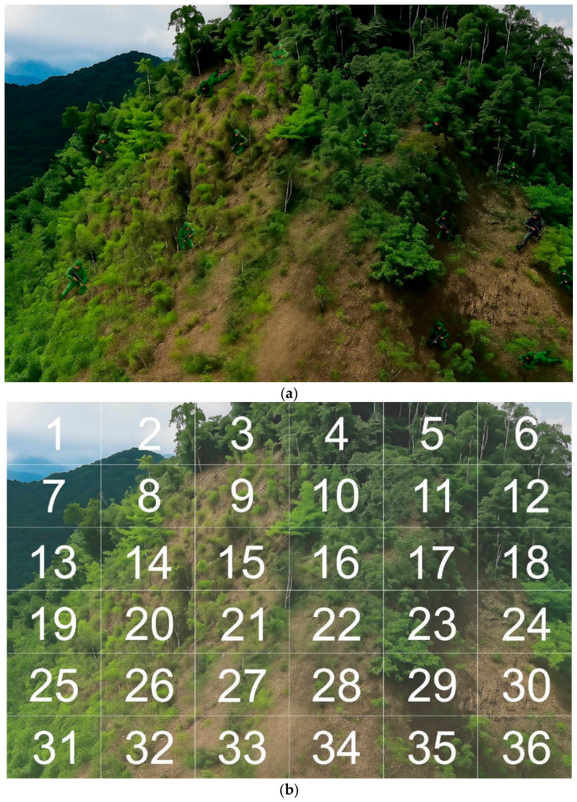
According to the search results of 52 participants viewing the wide-view images (Figure A1a), Blocks 1, 2, 7, and 13 were excluded from the primary ranking analysis because these regions mainly contained sky and steep cliff surfaces, which were not suitable areas for placing or concealing human figures in the simulated mountainous landscape. Among the remaining valid regions, lower identification frequency indicated stronger concealment performance. Samples A-4 and A-13 showed the lowest identification frequency, with only one identification each, and were therefore ranked jointly as the best-performing samples. Sample A-4 corresponded to A. scholaris leaf texture, whereas sample A-13 corresponded to T. mantaly leaf texture; both belonged to the dark green series. This result suggests that dark green camouflage samples achieved stronger visual integration with the mountainous background.
By contrast, the most easily identified regions were Block 8 (sample C-3, corresponding to F. microcarpa leaf texture), Block 14 (sample C-6, corresponding to A. scholaris leaf texture), and Block 24 (sample D-16, corresponding to the commonly used regional camouflage military uniform), each of which was identified six times. These were followed by Block 3 (sample C-15, corresponding to T. mantaly leaf texture) and Block 9 (sample C-9, corresponding to C. camphora leaf texture), which were each identified five times.
Overall, the high identification frequencies of C-3, C-6, C-15, and C-9 indicate that light green camouflage samples were more visually salient in the real wide-view mountainous scene. In addition, the high visibility of D-16 further confirms that the commonly used regional camouflage military uniform, as a conventional static reference sample, was more easily detected than the best-performing dark green samples developed in this study. These results indicate that darker camouflage samples, particularly A-4 and A-13, provided stronger concealment performance, whereas light green samples and the static regional reference camouflage showed weaker visual integration with the natural background.
Table A2.
Camouflage performance ranking based on identification frequency in the wide-view mountainous scene.
References
- Liu, Y.; Wang, C.-q.; Li, H.-p.; Zhou, Y.-j. Gait recognition of camouflaged people based on UAV infrared imaging. Infrared Phys. Technol. 2024, 138, 105262. [Google Scholar] [CrossRef] [Scilit]
- Li, Y.; Jia, C.; Liu, Y.; Duan, W.; Qing, X.; Zhang, J.; Weng, X. Evaluation of electrochromic film camouflage effect based on visual perception. Displays 2025, 89, 103066. [Google Scholar] [CrossRef] [Scilit]
- Lin, C.J.; Prasetyo, Y.T. A metaheuristic-based approach to optimizing color design for military camouflage using particle swarm optimization. Color Res. Appl. 2019, 44, 740–748. [Google Scholar] [CrossRef] [Scilit]
- Goudarzi, U.; Mokhtari, J.; Nouri, M. Camouflage of cotton fabrics in visible and NIR region using three selected vat dyes. Color Res. Appl. 2014, 39, 200–207. [Google Scholar] [CrossRef] [Scilit]
- Green, P. Colorimetry and colour difference. In Fundamentals and Applications of Colour Engineering; Green, P., Ed.; John Wiley & Sons: Hoboken, NJ, USA, 2023; pp. 27–52. [Google Scholar] [CrossRef] [Scilit]
- Ji, J.; Fang, S.; Shi, Z.; Xia, Q.; Li, Y. An efficient nonlinear polynomial color characterization method based on interrelations of color spaces. Color Res. Appl. 2020, 45, 1023–1039. [Google Scholar] [CrossRef] [Scilit]
- Ohta, N. Color Engineering: Theory and Application; Chuan Hwa Books: Taipei, Taiwan, 2008; pp. 115–134. [Google Scholar]
- Lin, C.J.; Prasetyo, Y.T.; Siswanto, N.D.; Jiang, B.C. Optimization of color design for military camouflage in CIE L*a*b* color space. Color Res. Appl. 2019, 44, 367–380. [Google Scholar] [CrossRef] [Scilit]
- Hsiao, S.-W.; Tsai, C.-J. Transforming the natural colors of an image into product design: A computer-aided color planning system based on fuzzy pattern recognition. Color Res. Appl. 2015, 40, 612–625. [Google Scholar] [CrossRef] [Scilit]
- Wan, M.; Zhao, D.; Zhao, B. Combining max pooling-Laplacian theory and k-means clustering for novel camouflage pattern design. Front. Neurorobot. 2022, 16, 1041101. [Google Scholar] [CrossRef] [Scilit] [PubMed]
- Wei, X.; Zhou, M.; Liu, B. Camouflage design of analysis based on HSV color statistics and k-means clustering. arXiv 2019, arXiv:1906.07968. [Google Scholar] [CrossRef] [Scilit]
- Cuthill, I.C.; Allen, W.L.; Arbuckle, K.; Caspers, B.; Chaplin, G.; Hauber, M.E.; Hill, G.E.; Jablonski, N.G.; Jiggins, C.D.; Kelber, A.; et al. The biology of color. Science 2017, 357, eaan0221. [Google Scholar] [CrossRef] [Scilit] [PubMed]
- Stevens, M.; Merilaita, S. Animal camouflage: Current issues and new perspectives. Philos. Trans. R. Soc. B 2009, 364, 423–427. [Google Scholar] [CrossRef] [Scilit] [PubMed]
- Itti, L.; Koch, C. Computational modelling of visual attention. Nat. Rev. Neurosci. 2001, 2, 194–203. [Google Scholar] [CrossRef] [Scilit] [PubMed]
- Karthiga, K.; Asuntha, A. A novel hybrid statistical model for camouflaged target detection. Int. J. Electr. Comput. Eng. 2025, 15, 1612–1619. [Google Scholar] [CrossRef] [Scilit]
- Umeton, D.; Tarawneh, G.; Fezza, E.; Read, J.C.A.; Rowe, C. Pattern and speed interact to hide moving prey. Curr. Biol. 2019, 29, 3109–3113.e3. [Google Scholar] [CrossRef] [Scilit] [PubMed]
- Troscianko, J.; Skelhorn, J.; Stevens, M. Quantifying camouflage: How to predict detectability from appearance. BMC Evol. Biol. 2017, 17, 7. [Google Scholar] [CrossRef] [Scilit] [PubMed]
- Song, Y.; Li, C.; Xiao, S.; Zhou, Q.; Xiao, H. A parallel Canny edge detection algorithm based on OpenCL acceleration. PLoS ONE 2024, 19, e0292345. [Google Scholar] [CrossRef] [Scilit] [PubMed]
- Daneshvar, E.; Tehran, M.A.; Zhang, Y.-J. Hybrid camouflage pattern generation using neural style transfer method. Color Res. Appl. 2022, 47, 878–891. [Google Scholar] [CrossRef] [Scilit]
- Yang, X.; Xu, W.-d.; Jia, Q.; Liu, J. MF-CFI: A fused evaluation index for camouflage patterns based on human visual perception. Def. Technol. 2021, 17, 1602–1608. [Google Scholar] [CrossRef] [Scilit]
- Hall, J.R.; Matthews, O.; Volonakis, T.N.; Liggins, E.; Lymer, K.P.; Baddeley, R.; Cuthill, I.C.; Scott-Samuel, N.E. A platform for initial testing of multiple camouflage patterns. Def. Technol. 2021, 17, 1833–1839. [Google Scholar] [CrossRef] [Scilit]
- Barnett, J.B.; McEwen, B.L.; Kinley, I.; Anderson, H.M.; Yeager, J. Behavioural mimicry among poison frogs diverges during close-range encounters with predators. J. Evol. Biol. 2025, 38, 663–671. [Google Scholar] [CrossRef] [Scilit] [PubMed]
- Barnett, J.B.; Cuthill, I.C. Distance-dependent defensive coloration. Curr. Biol. 2014, 24, R1157–R1158. [Google Scholar] [CrossRef] [Scilit] [PubMed]
- Cuthill, I.C.; Matchette, S.R.; Scott-Samuel, N.E. Camouflage in a dynamic world. Curr. Opin. Behav. Sci. 2019, 30, 109–115. [Google Scholar] [CrossRef] [Scilit]
- Brunyé, T.T.; Martis, S.B.; Kirejczyk, J.A.; Rock, K. Camouflage pattern features interact with movement speed to determine human target detectability. Appl. Ergon. 2019, 77, 50–57. [Google Scholar] [CrossRef] [Scilit] [PubMed]
- Van der Burg, E.; Hogervorst, M.A.; Toet, A. Adaptive camouflage for moving objects. J. Percept. Imaging 2021, 4, 020502. [Google Scholar] [CrossRef] [Scilit]
- Hashemi, S.; Ghaffarianhoseini, A.; Ghaffarianhoseini, A.; Naismith, N.; Santamouris, M.; Kikumoto, H. Pedestrian-level wind speed analysis: A case study. Archit. Sci. Rev. 2024, 68, 323–338. [Google Scholar] [CrossRef] [Scilit]
- Singleton, F. The Beaufort scale of winds—Its relevance, and its use by sailors. Weather 2008, 63, 37–41. [Google Scholar] [CrossRef] [Scilit]
- Niklas, K.J. The influence of gravity and wind on land plant evolution. Rev. Palaeobot. Palynol. 1998, 102, 1–14. [Google Scholar] [CrossRef] [Scilit] [PubMed]
- Wolfe, J.M.; Horowitz, T.S. Five factors that guide attention in visual search. Nat. Hum. Behav. 2017, 1, 0058. [Google Scholar] [CrossRef] [Scilit] [PubMed]
- Henderson, J.M. Human gaze control during real-world scene perception. Trends Cogn. Sci. 2003, 7, 498–504. [Google Scholar] [CrossRef] [Scilit] [PubMed]
- Denning, R.J. Camouflage fabrics. In Engineering of High-Performance Textiles; Miao, M., Xin, J.H., Eds.; Woodhead Publishing: Duxford, UK, 2018; pp. 349–375. [Google Scholar] [CrossRef] [Scilit]
- Lin, Y.; Ren, L.; Yang, X.; Yuan, H. Design and application of bionic camouflage materials simulating spectral reflection characteristics of plants: A review. Appl. Sci. 2024, 14, 4404. [Google Scholar] [CrossRef] [Scilit]
- Brunyé, T.T.; Eddy, M.D.; Cain, M.S.; Hepfinger, L.B.; Rock, K. Masked priming for the comparative evaluation of camouflage conspicuity. Appl. Ergon. 2017, 62, 259–267. [Google Scholar] [CrossRef] [Scilit] [PubMed]
- Torrico, D.D.; Fuentes, S.; Gonzalez Viejo, C.; Ashman, H.; Gurr, P.A.; Dunshea, F.R. Analysis of thermochromic label elements and colour transitions using sensory acceptability and eye tracking techniques. LWT 2018, 89, 475–481. [Google Scholar] [CrossRef] [Scilit]
- Husić-Mehmedović, M.; Omeragić, I.; Batagelj, Z.; Kolar, T. Seeing is not necessarily liking: Advancing research on package design with eye-tracking. J. Bus. Res. 2017, 80, 145–154. [Google Scholar] [CrossRef] [Scilit]
- Park, S.-Y.; Kang, T.-W.; Koo, D.-K. Investigating eye movement and postural stability relationships using mobile eye-tracking and posturography: A cross-sectional study. Bioengineering 2024, 11, 742. [Google Scholar] [CrossRef] [Scilit] [PubMed]
- Gamino-Sánchez, F.; Hernández-Gutiérrez, I.V.; Rosales-Silva, A.J.; Gallegos-Funes, F.J.; Mújica-Vargas, D.; Ramos-Díaz, E.; Carvajal-Gámez, B.E.; Kinani, J.M.V. Block-matching fuzzy c-means clustering algorithm for segmentation of color images degraded with Gaussian noise. Eng. Appl. Artif. Intell. 2018, 73, 31–49. [Google Scholar] [CrossRef] [Scilit]
- R Core Team. R: A Language and Environment for Statistical Computing, Version 4.5.1; R Foundation for Statistical Computing: Vienna, Austria, 2025; Available online: https://www.R-project.org/ (accessed on 1 November 2025).
- Central Weather Administration (CWA). Annual Weather Forecast Report 2023; Central Weather Administration: Taipei, Taiwan, 2025. Available online: https://www.cwa.gov.tw/Data/service/notice/download/Publish_20250326113535.pdf (accessed on 1 November 2025).
- Wei, C.-C.; Peng, P.-C.; Tsai, C.-H.; Huang, C.-L. Regional forecasting of wind speeds during typhoon landfall in Taiwan: A case study of westward-moving typhoons. Atmosphere 2018, 9, 141. [Google Scholar] [CrossRef] [Scilit]
- World Meteorological Organization. Guide to Meteorological Instruments and Methods of Observation, 7th ed.; WMO-No. 8; World Meteorological Organization: Geneva, Switzerland, 2012. [Google Scholar]
- Sun, Z.; Cui, T.; Zhu, Y.; Zhang, W.; Shi, S.; Tang, S.; Du, Z.; Liu, C.; Cui, R.; Chen, H.; et al. The mechanical principles behind the golden ratio distribution of veins in plant leaves. Sci. Rep. 2018, 8, 13859. [Google Scholar] [CrossRef] [Scilit] [PubMed]
- LeCun, Y.; Bottou, L.; Bengio, Y.; Haffner, P. Gradient-based learning applied to document recognition. Proc. IEEE 1998, 86, 2278–2324. [Google Scholar] [CrossRef] [Scilit]
- Krizhevsky, A.; Sutskever, I.; Hinton, G.E. ImageNet classification with deep convolutional neural networks. In Advances in Neural Information Processing Systems 25; Pereira, F., Burges, C.J.C., Bottou, L., Weinberger, K.Q., Eds.; Curran Associates: Red Hook, NY, USA, 2012; pp. 1097–1105. [Google Scholar]
- Simonyan, K.; Zisserman, A. Very deep convolutional networks for large-scale image recognition. arXiv 2014, arXiv:1409.1556. [Google Scholar] [CrossRef] [Scilit]
- He, K.; Zhang, X.; Ren, S.; Sun, J. Deep residual learning for image recognition. In Proceedings of the 2016 IEEE Conference on Computer Vision and Pattern Recognition (CVPR), Las Vegas, NV, USA, 27–30 June 2016; pp. 770–778. [Google Scholar] [CrossRef] [Scilit]
- Faul, F.; Erdfelder, E.; Lang, A.-G.; Buchner, A. G*Power 3: A flexible statistical power analysis program for the social, behavioral, and biomedical sciences. Behav. Res. Methods 2007, 39, 175–191. [Google Scholar] [CrossRef] [Scilit] [PubMed]
- Beatty, J. Task-evoked pupillary responses, processing load, and the structure of processing resources. Psychol. Bull. 1982, 91, 276–292. [Google Scholar] [CrossRef]
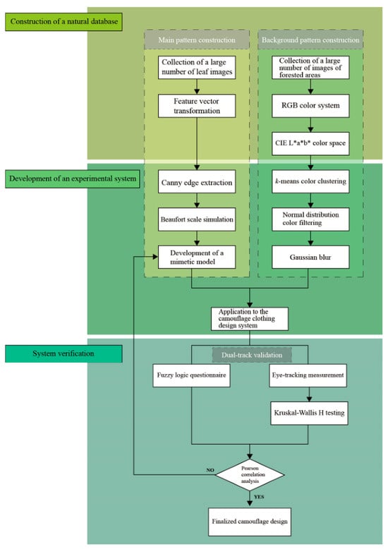
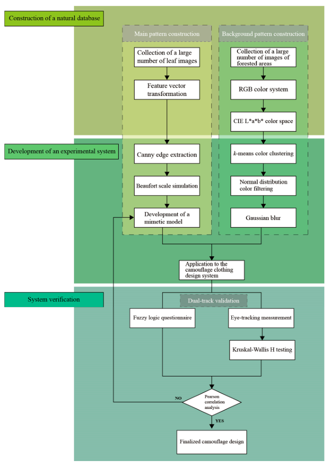
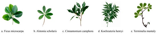
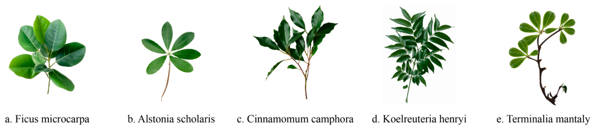
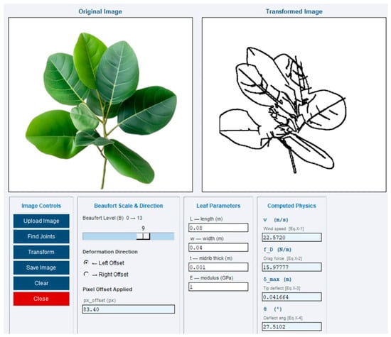
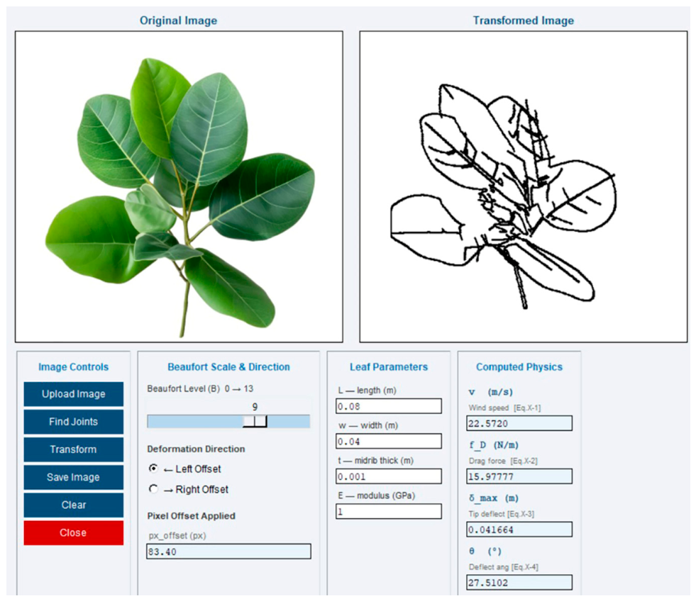
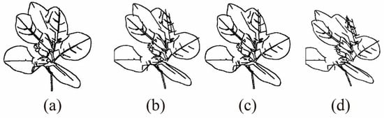
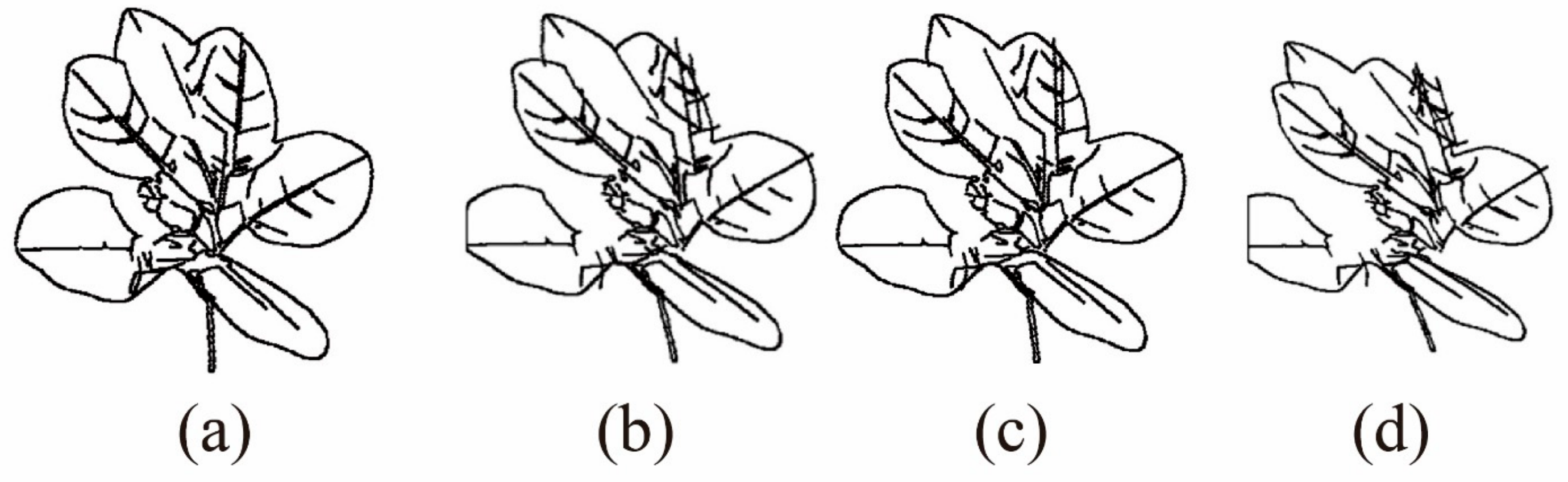
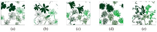
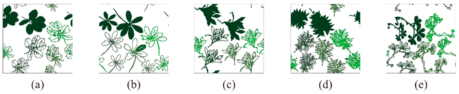
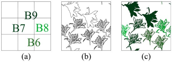
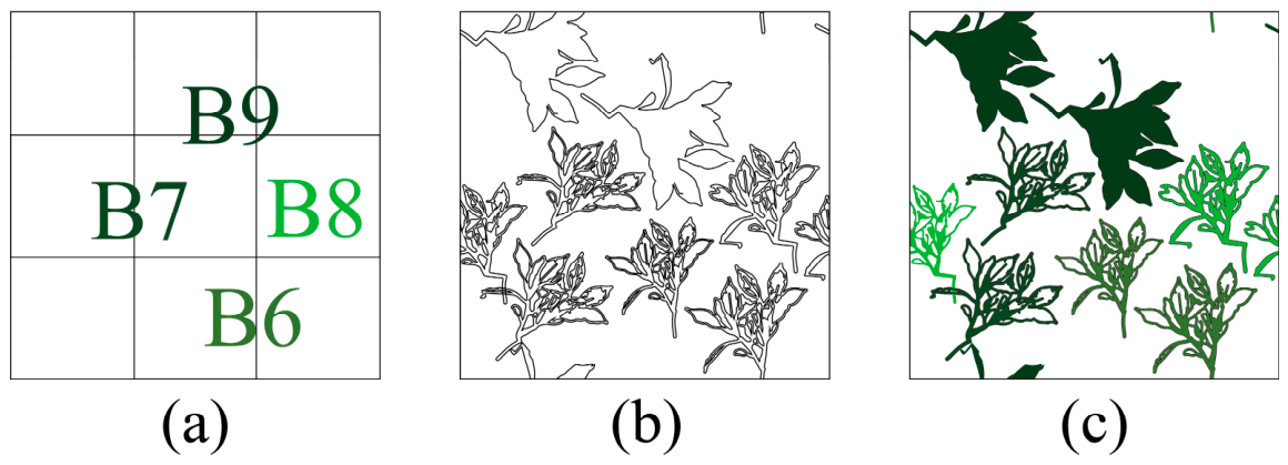
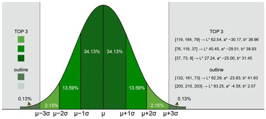
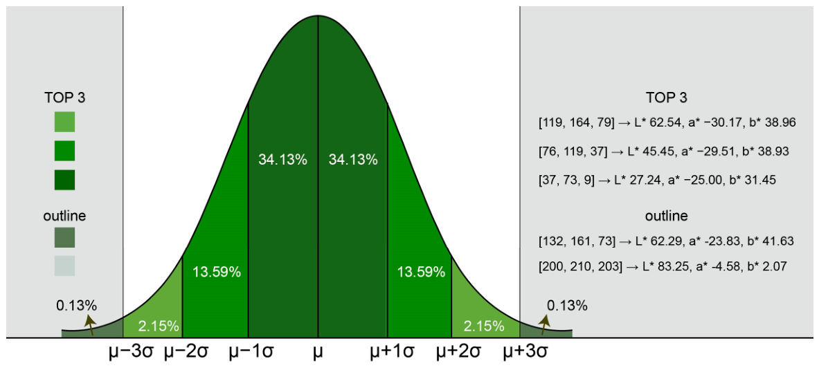
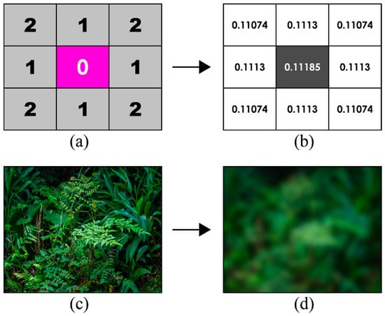
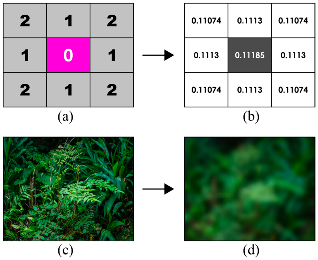
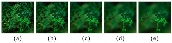
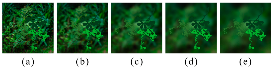
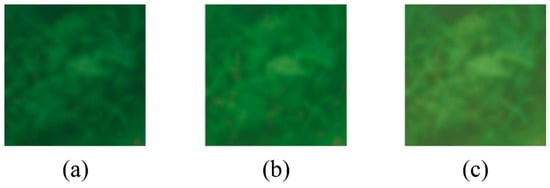
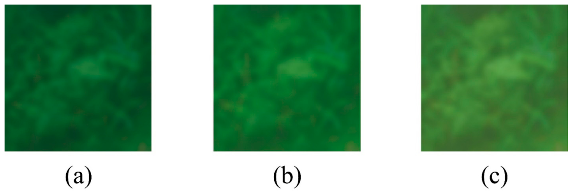
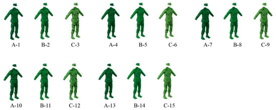
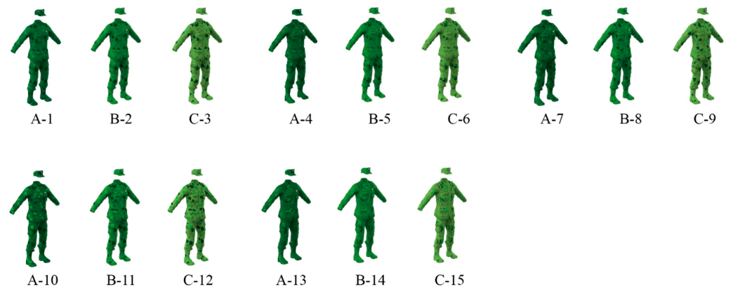
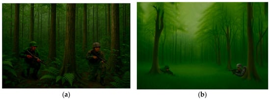
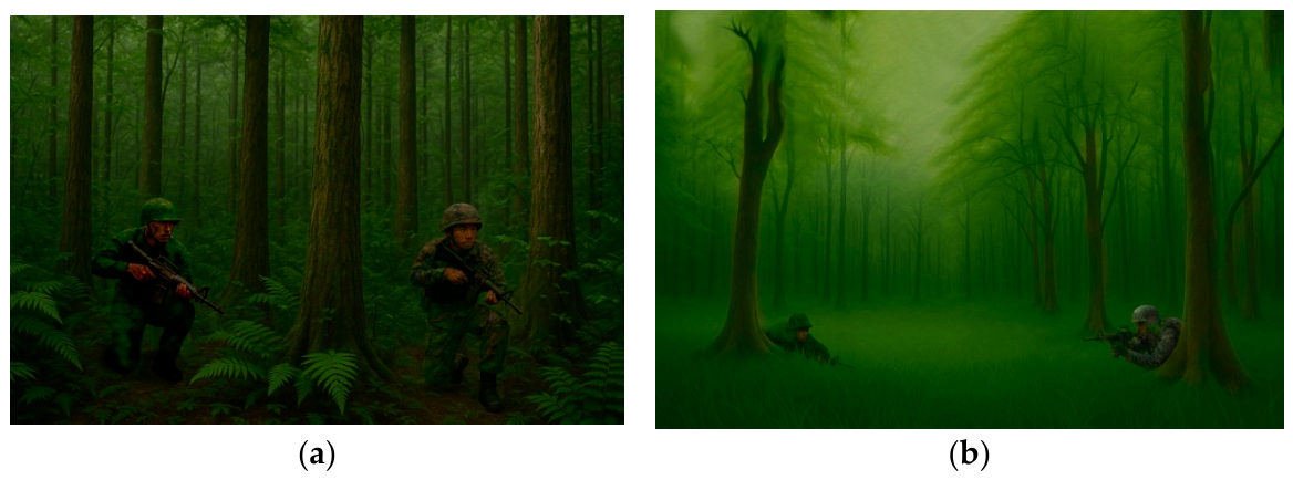
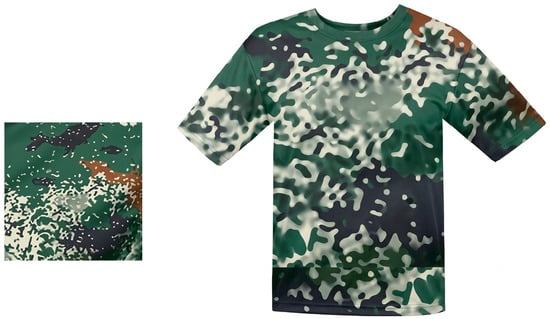
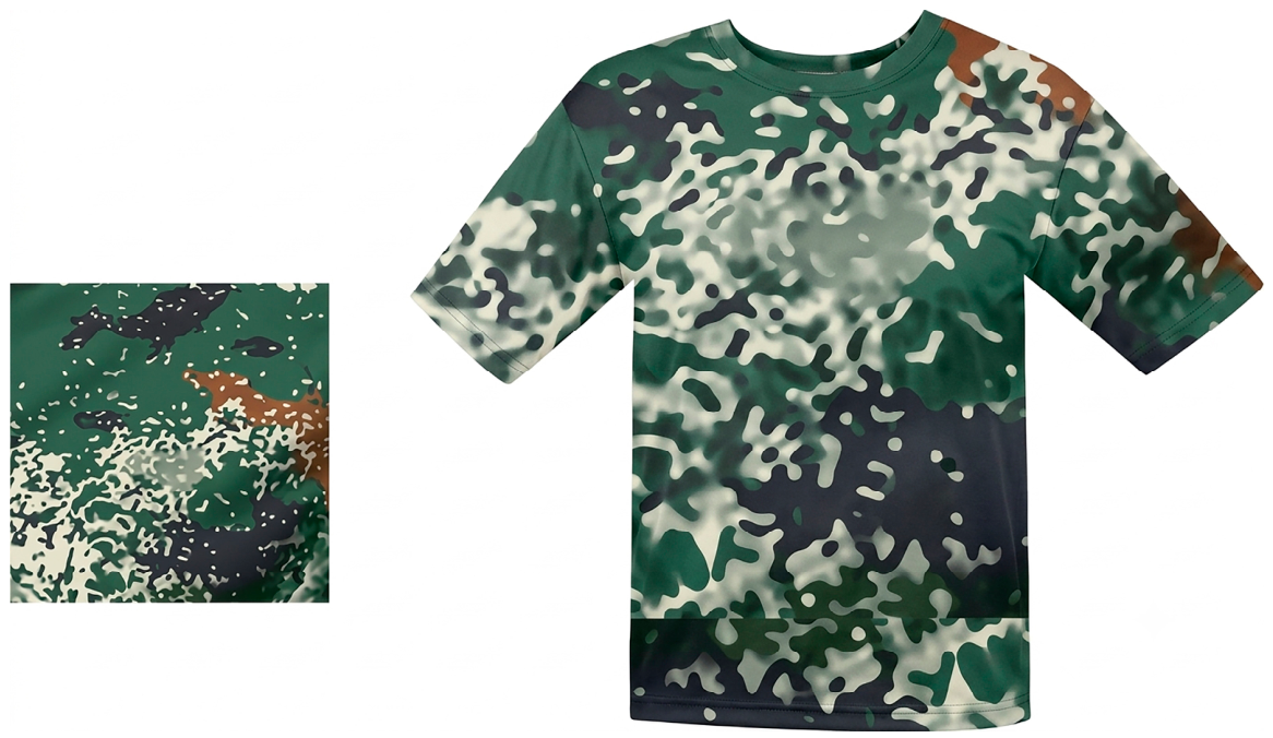
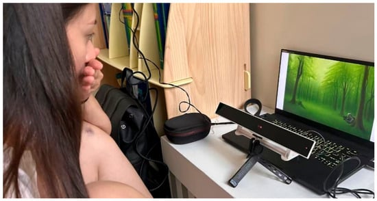
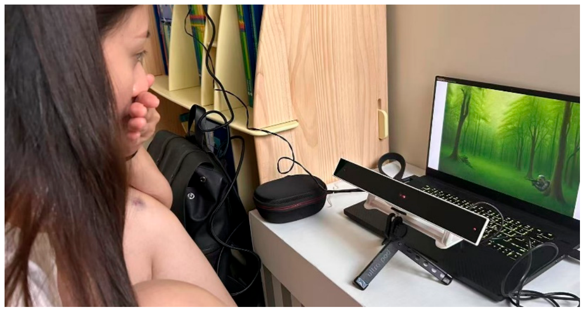
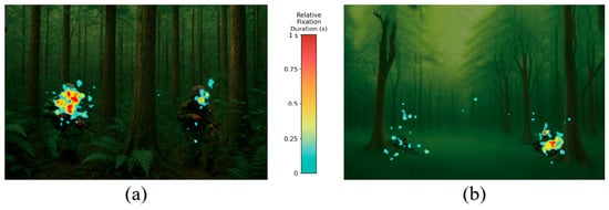
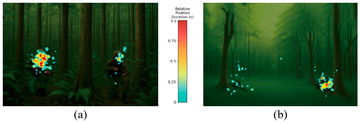
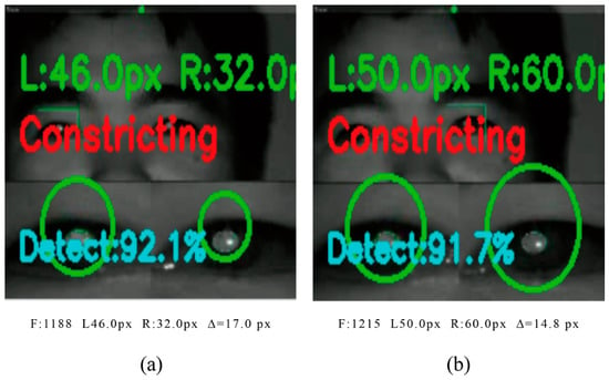
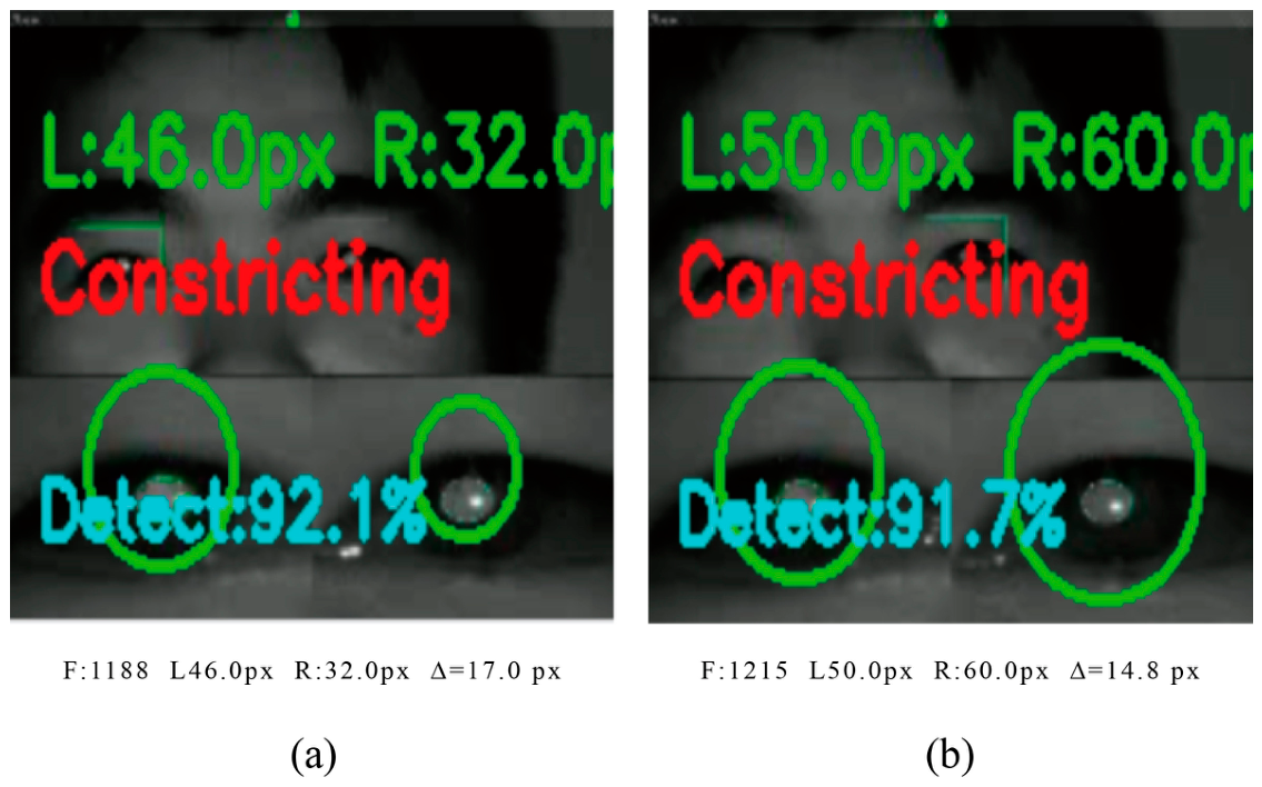
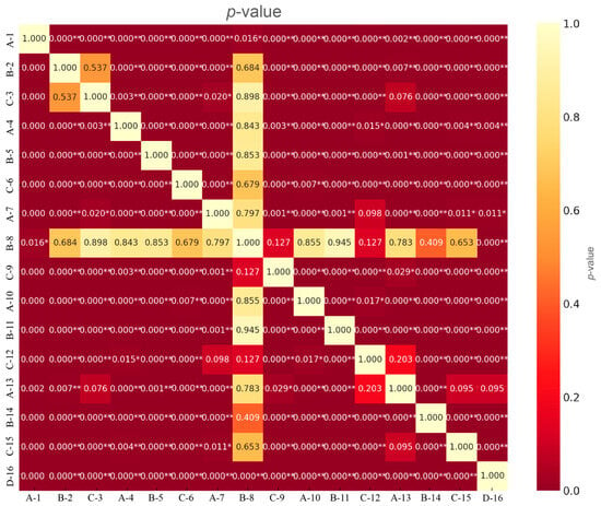
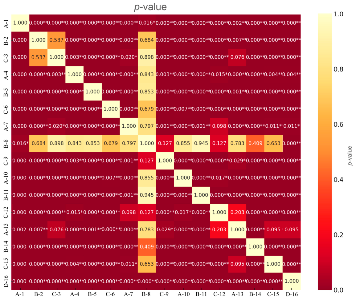

Disclaimer/Publisher’s Note: The statements, opinions and data contained in all publications are solely those of the individual author(s) and contributor(s) and not of MDPI and/or the editor(s). MDPI and/or the editor(s) disclaim responsibility for any injury to people or property resulting from any ideas, methods, instructions or products referred to in the content. |
© 2026 by the authors. Licensee MDPI, Basel, Switzerland. This article is an open access article distributed under the terms and conditions of the Creative Commons Attribution (CC BY) license.