A Coordinated Planning Method for Flexible Distribution Networks Oriented Toward Power Supply Restoration and Resilience Enhancement

Abstract

In recent years, the increasing frequency of extreme weather events, the large-scale integration of distributed generation into distribution networks, and the widespread application of new power electronic devices have posed severe challenges to the security of power supply in distribution networks. To enhance the power supply reliability of the distribution network while considering its economic efficiency, this paper proposes a collaborative planning method for a flexible distribution network focused on power supply restoration and resilience enhancement In this method, a planning model for flexible distribution networks is established by optimally determining the siting and sizing of soft open point (SOP), with the objective of minimizing the annual comprehensive cost of the distribution network under multiple operational and planning constraints. Second-order cone programming (SOCP) relaxation and polyhedral approximation-based linearization techniques are employed to reformulate and solve the model, thereby obtaining the optimal siting and sizing Case for SOPs. Finally, simulations are conducted on a modified IEEE 33-bus test system to verify the effectiveness of the proposed method. The results show that, through appropriate siting and sizing of SOPs, outage loss costs can be significantly reduced, nodal voltage profiles can be improved, and load support can be provided to de-energized areas, leading to a reduction of more than 70% in the annual comprehensive cost of the distribution network and an improvement in the system reliability index from 99% to 99.999%, thus effectively enhancing both the economic efficiency and reliability of the distribution system.

1. Introduction

In recent years, owing to climate change and the increasing frequency of extreme weather events, natural disasters such as typhoons [1,2], heavy rainfall [3,4], heat waves [5,6], and snow and ice storms [7,8] have had an increasingly significant impact on power systems. Meanwhile, the large-scale integration of new energy sources such as distributed photovoltaic (PV) generation and the widespread application of various emerging power electronic devices [9] have drastically changed the operating characteristics of distribution networks, with outages occurring from time to time and posing severe challenges to their secure operation. As the primary interface linking the power system to end users, the distribution network must prioritize reliability. Thus, enhancing power supply reliability is a core objective in its planning and construction, directly impacting customer service quality. However, conventional distribution networks are large in scale, characterized by aging infrastructure and complex structures [10]; once a wide-area outage occurs, it can lead to enormous economic losses and severe social impacts, greatly undermining the supply reliability of distribution networks. Therefore, improving the power supply reliability of distribution networks is of great significance.

The soft open point (SOP) is a power electronic device that follows the principle of “closed-loop design and open-loop operation” and is typically used to replace traditional tie switches. Its capability of seamless, stepless regulation of power exchange enables precise power-flow control between feeders, thereby facilitating flexible closed-loop operation of distribution networks. In the event of a fault, the SOP can effectively block the propagation of fault currents, expand the scope of service restoration, and enhance the supply reliability of distribution networks [11]. With respect to the application of SOPs in distribution systems, Reference [11] investigates SOP-based fault scenarios in distribution networks, elaborating on their voltage support capability for outage areas and their ability to improve system load restoration, thus extending the restoration range of the distribution network. Reference [12] proposes a fault restoration strategy for distribution networks using SOPs in coordination with distributed generation; however, the SOP capacities and restoration Cases are fixed, making it difficult to achieve effective restoration under fault conditions. Building on fault restoration, Reference [13] develops an equivalent SOP model for reliability assessment and proposes a reliability evaluation framework for flexible distribution networks based on decoupled modeling of the multi-stage restoration process, thereby verifying the great potential of SOPs in supply restoration of distribution networks. Reference [14] explicitly integrates analytical reliability expressions into a multi-type switch configuration model for flexible distribution networks, where the deployment is determined by trading off annualized switch-related costs and outage-induced economic loss while meeting reliability requirements. The above studies provide a useful reference for research on SOP-based fault restoration in distribution networks and demonstrate that SOPs can improve the supply reliability of distribution networks to a certain extent; however, they do not take into account the impact of SOPs on the economic performance of distribution networks.

Reference [15] proposes a bi-level planning framework for distribution networks that considers the coordinated operation of distributed generation (DG), energy storage systems (ESS), and SOPs, where the capacities and locations of SOPs are optimized to reduce the total investment and operating costs. In [16], flexible resources such as SOPs, ESS, and line reinforcement are deployed in a pre-disaster manner to enhance the resilience of distribution networks and reduce losses caused by typhoon events, thereby verifying the effectiveness of SOPs and other flexible resources in improving grid resilience; although the economic performance of the distribution network is considered, reliability indices are not evaluated. Reference [17] adopts a branch failure rate calculation method based on correlation constraints for SOP-based networks and proposes an SOP planning method for distribution networks that accounts for reliability benefits, but the optimal capacities of SOPs are not determined. Reference [18] presents a supply restoration method based on the coordination of multiple SOPs to enhance the self-healing capability of active distribution networks (ADNs); it addresses the siting and sizing of SOPs and computes reliability indices, yet does not consider the economic performance of the distribution network. Reference [19] proposes a distributed supply restoration method for smart distribution networks with intelligent SOPs and develops output adjustment strategies that satisfy distributed restoration requirements under different SOP control modes. Reference [20] investigates the impact of a four-terminal SOP on distribution network reliability and supply restoration capability, and establishes a corresponding supply capability evaluation model. At present, few studies simultaneously consider the economic performance of distribution networks and the calculation of reliability indices, and the constructed models of flexibly interconnected distribution networks are highly nonlinear and thus difficult to solve directly.

To address the above issues, this paper proposes a coordinated planning method for flexible distribution networks oriented toward power supply restoration and resilience enhancement. First, a flexible distribution network planning model is established with the objective of minimizing the annual comprehensive cost of the flexibly interconnected distribution network, while simultaneously considering the siting and sizing of SOPs and evaluating system supply reliability indices. Second, in view of the nonlinear characteristics of the proposed model, second-order cone relaxation and a polyhedral approximation method are employed to obtain an equivalent reformulation, which significantly reduces the computational complexity of the model. Finally, the proposed method is validated through comparative studies on a modified IEEE 33-bus test system, from which the optimal SOP siting and sizing Case is obtained, thereby demonstrating the effectiveness of the proposed approach.

2. Flexibly Interconnected Distribution Network Model

This section elaborates on the mathematical framework for the coordinated planning of flexible distribution networks. To begin, Section 2.1 details the structure of the flexible distribution network, particularly focusing on the integration of Soft Open Points (SOPs). Then, we will formulate the optimization objective and operational constraints essential for enhancing resilience.

2.1. Flexible Interconnected Distribution Network Structure

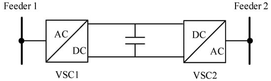
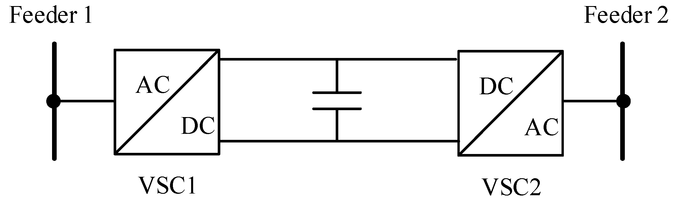
In this paper, the SOP is a fully controllable power electronic device, and the basic configuration of a back-to-back voltage-source-converter-based SOP is shown in Figure 1. The model consists of two voltage source converters (VSCs), VSC1 and VSC2, connected in a back-to-back arrangement [21]. Under normal operating conditions, VSC1 controls power transfer, while VSC2 regulates the DC-link voltage. The two VSCs can flexibly regulate both active and reactive power, thereby controlling the power flows and voltage profiles in the system.

Figure 1. Back-to-back voltage-source-converter-based SOP.

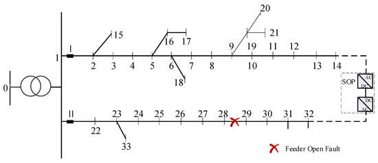
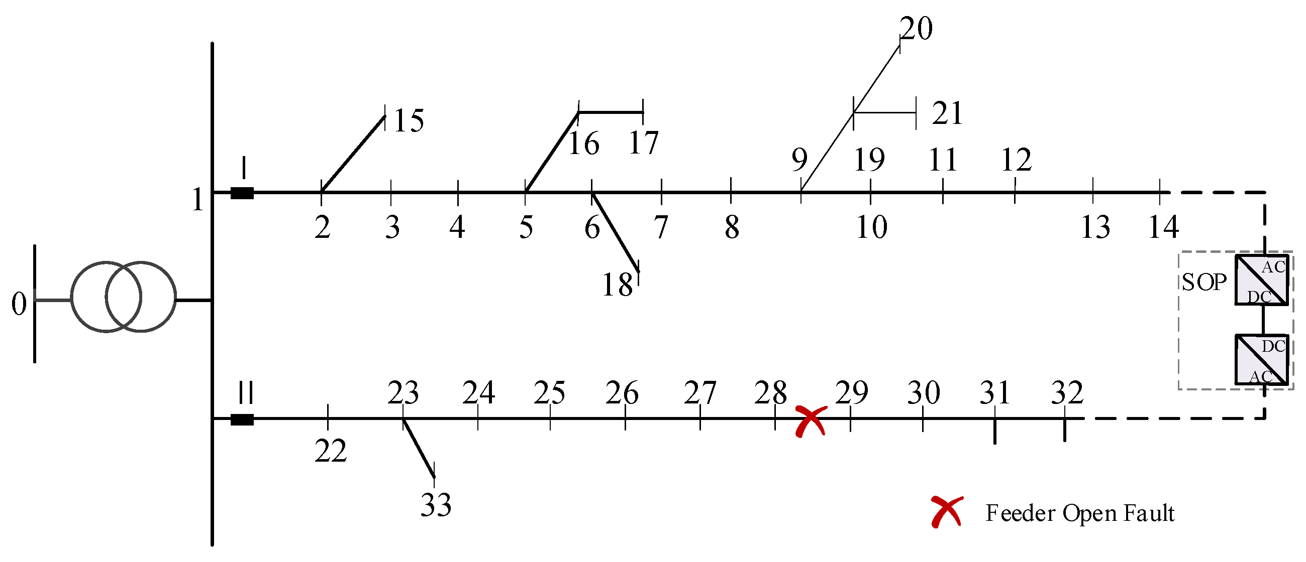
Based on the SOP described above, a flexibly interconnected distribution system is investigated, and its topology is shown in Figure 2. The distribution network consists of two feeders, labelled I and II in the figure. The SOP is installed between bus 14 of feeder I and bus 32 of feeder II, as indicated by the dashed box at the right-hand side of the figure. The red “×” symbol on branch 28–29 marks the location of the feeder open fault considered in this case. One terminal of the SOP is connected to the outage area to provide voltage and power support, while the other terminal is connected to the non-outage area to obtain active power support. By rapidly and accurately controlling the transfer of active and reactive power through the SOP, power supply restoration in the distribution network can be maximized.

Figure 2. Flexible interconnected distribution network structure.

The integration of the SOP modifies the original topology of the distribution network, transforming it from a network interconnected by conventional tie switches into a flexible distribution network interconnected via a DC ring. In this way, while maintaining the open-loop operating characteristics of a radial structure, the distribution network further acquires the high reliability of a ring network, thereby achieving a coordinated enhancement of operational flexibility and supply reliability.

2.2. Planning Model

The planning objective for the flexible distribution network aims to achieve a coordinated optimization of both economic efficiency and resilience by minimizing the annual comprehensive cost. This section details the formulation of the integrated objective function, which includes investment, O&M, network loss, and outage loss costs.

2.2.1. Annual Investment and O&M Costs of SOPs

Considering that SOPs continue to function throughout their entire economic lifetime after the initial construction investment, the one-off capital cost needs to be converted into an equivalent annual investment cost so as to facilitate consistent economic comparison and planning. In addition, once SOPs are put into operation, they incur annual operation and maintenance (O&M) expenses. The corresponding cost components are given in (1) and (2).

$$C^{\mathrm{sop},\mathrm{inv}}={\tau }^{\mathrm{SOP}}{\displaystyle \sum _{i\in {\mathsf{\Omega }}_{\mathrm{SOP}}}{c}^{\mathrm{sop}}{S}_i^{\mathrm{sop}}}$$

(1)

$$C^{\mathrm{om}}=\gamma {\displaystyle \sum _{i\in {\mathsf{\Omega }}_{\mathrm{SOP}}}{c}^{\mathrm{sop}}{S}_i^{\mathrm{sop}}}$$

(2)

Here, $C^{\mathrm{sop},\mathrm{inv}}$ and $C^{\mathrm{om}}$ represent the annualized investment cost of SOPs and the annual operation and maintenance (O&M) cost of SOPs, respectively; ${\Omega }_{\mathrm{SOP}}$ represents the set of candidate nodes for SOP planning. $c^{\mathrm{sop}}$ represents the unit-capacity investment cost of SOPs. $S_i^{\mathrm{sop}}$ represents the capacity of SOP installed at node i; $\gamma$ represents the O&M cost rate; ${\tau }^{\mathrm{SOP}}$ represents the coefficient for converting the planning value of equipment into an equivalent annual value, which is calculated as follows:

$${\tau }^{\mathrm{SOP}}=r{\displaystyle \frac{{(1+r)}^y}{{(1+r)}^y-1}}$$

(3)

where $r$ represents the discount rate, and $y$ represents the fixed investment recovery period of the SOP.

2.2.2. Annual Network Loss Cost and Outage Loss Cost of the Distribution Network

For a given SOP planning case, the annual network loss cost and the outage loss cost of the distribution network can be evaluated as follows:

$$C^{\mathrm{L}}=365c^{\mathrm{p}}{\displaystyle \sum _{t\in {\mathsf{\Omega }}_{TN}}({\displaystyle \sum _{ij\in {\mathsf{\Omega }}_1}{r}_{ij}{I}_{ij,t}^2}+{\displaystyle \sum _{i\in {\mathsf{\Omega }}_{\mathrm{SOP}}}{P}_{i,t}^{\mathrm{SOP},\mathrm{L}}})}$$

(4)

$$C^{\mathrm{R}}=c^{\mathrm{I}}{\displaystyle \sum _{t\in T}{\displaystyle \sum _{i\in {\mathsf{\Omega }}_n}(1-{\mu }_i)P_{i,t}^{\mathrm{LOAD}}\Delta \mathrm{t}}}$$

(5)

where $C^{\mathrm{L}}$ and $C^{\mathrm{R}}$ represent the annual network loss cost and the outage loss cost of the distribution network, respectively; $c^{\mathrm{p}}$ and $c^{\mathrm{I}}$ represent the unit outage loss cost and the unit electricity price, respectively; ${\mathsf{\Omega }}_1$ and ${\mathsf{\Omega }}_{\mathrm{TN}}$ represent the set of all lines and the set of time periods in a typical day, respectively; ${\mathsf{\Omega }}_{\mathrm{sop}}$ and ${\mathsf{\Omega }}_{\mathrm{n}}$ represent the set of candidate nodes for SOP planning and the set of all nodes. $\Delta \mathrm{t}$ is the fault duration. $r_{ij}$ is the resistance of branch ij; $I_{ij,t}$ is the current of branch ij at time t; ${\mu }_i$ is the load coefficient at recoverable load node i; ${\mu }_i\in [0,1]$; $P_{i,t}^{\mathrm{LOAD}}$ and $P_{i,t}^{\mathrm{SOP},\mathrm{L}}$ represent the active power consumed by the load at node i and the active power loss of the SOP at node i at time t, respectively.

2.2.3. Objective Function

In this paper, the annual comprehensive cost of the flexibly interconnected distribution network is taken as the objective function. It mainly consists of the annualized planning investment cost of SOPs, the annual operation and maintenance (O&M) cost of SOPs, the annual network loss cost of the distribution network, and the annual outage loss cost of loads. From an economic perspective, the total cost is required to be minimized. By converting the up-front planning investment cost into an equivalent annual value, the total planning cost is evaluated on an annual basis as follows:

$$\min C^{\mathrm{total}}=C^{\mathrm{sop},\mathrm{inv}}+C^{\mathrm{om}}+C^{\mathrm{L}}+C^{\mathrm{R}}$$

(6)

where $C^{\mathrm{total}}$ represents the annual comprehensive cost of the flexibly interconnected distribution network over a one-year period.

2.3. Constraints

The operational constraints of the system mainly include distribution network power flow constraints, voltage magnitude constraints, current magnitude constraints, SOP capacity and power constraints, and PV capacity constraints.

2.3.1. Power Flow Constraints

Since the network topology of the distribution network changes frequently, the power flow equations are relaxed by introducing line switching (open/close) variables, yielding the following DistFlow power flow equations:

$$\left\{\begin{array}{l}{\displaystyle \sum _{ij\in {\mathsf{\Omega }}_1}{\alpha }_{ij}(P_{ij,t}-I_{ij,t}^2{r}_{ij})}={\displaystyle \sum _{jk\in {\mathsf{\Omega }}_1}{\alpha }_{jk}{P}_{jk,t}+P_{j,t}}\\ {\displaystyle \sum _{ij\in {\mathsf{\Omega }}_1}{\alpha }_{ij}(Q_{ij,t}-I_{ij,t}^2{x}_{ij})}={\displaystyle \sum _{jk\in {\mathsf{\Omega }}_1}{\alpha }_{jk}{Q}_{jk,t}+Q_{j,t}}\end{array}\right.$$

(7)

$$\left\{\begin{array}{l}{P}_{j,t}=-P_{j\in {\mathsf{\Omega }}_{\mathrm{PV}}}^{\mathrm{PV}}-P_{j\in {\mathsf{\Omega }}_{\mathrm{SOP}}}^{\mathrm{SOP}}+{\mu }_i{P}_{j,t}^{\mathrm{load}}\\ Q_{j,t}=-Q_{j\in {\mathsf{\Omega }}_{\mathrm{PV}}}^{\mathrm{PV}}-Q_{j\in {\mathsf{\Omega }}_{\mathrm{SOP}}}^{\mathrm{SOP}}+{\mu }_i{Q}_{j,t}^{\mathrm{load}}\end{array}\right.$$

(8)

$$\begin{array}{c}{V}_{j,t}^2=V_{i,t}^2-2(r_{ij}{P}_{ij,t}+x_{ij}{Q}_{ij,t})+(r_{ij}^2+x_{ij}^2)I_{ij,t}^2\\ \forall ij\in {\mathsf{\Omega }}_1,{\alpha }_{ij}=1\end{array}$$

(9)

$$\begin{array}{l}{I}_{ij,t}^2{V}_{i,t}^2=P_{ij,t}^2+Q_{ij,t}^2\\ \forall ij\in {\mathsf{\Omega }}_1,{\alpha }_{ij}=1\end{array}$$

(10)

where ${\alpha }_{ij}$ and ${\alpha }_{jk}$ are 0–1 variables indicating the open/closed status of branch ij, taking the value 1 when branch ij is closed; $P_{ij,t}$ and $Q_{ij,t}$ represent the active and reactive power flowing through branch ij at time t; $x_{ij}$ is the reactance of branch ij; $P_{j,t}$ and $Q_{j,t}$ represent the active and reactive power injected at node j at time t; $P_{j,t}^{\mathrm{load}}$ and $Q_{j,t}^{\mathrm{load}}$ represent the active and reactive power consumed by the load injected at node j at time t; $P_{j,t}^{PV}$ and $Q_{j,t}^{PV}$ represent the active and reactive power injected by the PV unit at node j at time t; $P_{j,t}^{\mathrm{SOP}}$ and $Q_{j,t}^{\mathrm{SOP}}$ represent the active power transferred by the SOP at node j and the reactive power injected by the SOP at node j at time t, respectively; $I_{ij,t}$ is the magnitude of the current flowing through branch ij at time t; $V_{j,t}$ is the voltage magnitude at node j at time t.

2.3.2. Voltage Magnitude Constraints

Since the power flow equations may have multiple solutions, voltage magnitude and current magnitude constraints are imposed to confine the power flow solution within the normal operating range.

$$V_{j,t}^{\min }\le V_{j,t}\le V_{j,t}^{\max }$$

(11)

where $V_{j,t}^{\min }$ and $V_{j,t}^{\max }$ represent the minimum and maximum allowable voltage magnitudes at node j at time t, respectively.

2.3.3. Current Magnitude Constraints

The magnitude of the current flowing through each branch must not exceed its rated limit.

$$0\le I_{ij,t}^2\le {(I_{ij,t}^{\max })}^2$$

(12)

where $I_{ij,t}^{\max }$ denotes the maximum allowable current flowing through branch ij at time t.

2.3.4. SOP Capacity and Power Constraints

Under normal operating conditions, the active power and capacity constraints at both terminals of the SOP are given by

$$0\le S_i^{\mathrm{sop}}\le S_{\max }^{\mathrm{sop}}$$

(13)

$$P_{i,t}^{\mathrm{SOP}}+P_{i,t}^{\mathrm{SOP},\mathrm{L}}+P_{j,t}^{\mathrm{SOP}}+P_{j,t}^{\mathrm{SOP},\mathrm{L}}=0$$

(14)

$$P_{i,t}^{\mathrm{SOP},\mathrm{L}}=A_i^{\mathrm{SOP}}\sqrt{{(P_{i,t}^{\mathrm{SOP}})}^2+{(Q_{i,t}^{\mathrm{SOP}})}^2}$$

(15)

$${(P_{i,t}^{\mathrm{SOP}})}^2+{(Q_{i,t}^{\mathrm{SOP}})}^2\le {(S_i^{\mathrm{SOP}})}^2$$

(16)

$${(P_{j,t}^{\mathrm{SOP}})}^2+{(Q_{j,t}^{\mathrm{SOP}})}^2\le {(S_{ij}^{\mathrm{SOP}})}^2$$

(17)

where i and j denote the feeder indices at the two terminals of the SOP; $S_{\max }^{SOP}$ represents the upper limit of the installed SOP capacity; and $A_i^{\mathrm{SOP}}$ represents the power loss coefficient of the SOP, which is usually set to 0.02.

2.3.5. PV Capacity Constraints

The active power output of each PV unit is also restricted within its minimum and maximum available values.

$$P_{i,t}^{\mathrm{pv},\min }\le P_{i,t}^{\mathrm{pv}}\le P_{i,t}^{\mathrm{pv},\max }$$

(18)

where $P_{i,t}^{\mathrm{pv},\min }$ and $P_{i,t}^{\mathrm{pv},\max }$ represent the lower and upper limits of the PV output, respectively.

2.4. System Reliability Indices

Power supply reliability represents the ability of the power supply system to continuously deliver electricity to customers. The reliability indices of the system correspond to the reliability indices of load points and are usually classified into frequency-related indices and interruption-related (outage) indices:

The System Average Interruption Duration Index (SAIDI) represents the average outage duration per customer over one year, and is calculated as follows:

$$\mathrm{SAIDI}={\displaystyle \frac{\mathrm{Total} \mathrm{customer} \mathrm{interruption} \mathrm{duration}}{\mathrm{Total} \mathrm{number} \mathrm{of} \mathrm{customers}}}$$

(19)

The expected energy not supplied (EENS) represents the total amount of load energy that cannot be supplied by the grid during a one-year operating period due to system failures, and is calculated as follows:

$$\mathrm{EENS}=\mathrm{Total} \mathrm{system} \mathrm{outage} \mathrm{energy}$$

(20)

The Average Service Availability Index (ASAI) represents the availability of the distribution system and is calculated as follows:

$$\mathrm{ASAI}=1-{\displaystyle \frac{\mathrm{SAIDI}}{8760}}$$

(21)

3. Model Reformulation and Solution

In this section, the nonlinear power-flow and operational constraints are linearized by introducing auxiliary variables and appropriate relaxation techniques. On this basis, the overall problem is recast as a mixed-integer programming (MIP) model, and the corresponding solution procedure is described.

3.1. Linearization

The formulated model contains nonlinear constraints, which need to be transformed using convex relaxation and linearization techniques.

(1)

Power Flow Constraints

The power flow constraints given in Equations (7)–(10) form a non-convex model, and constraints (9) and (10) are only valid for closed branches (${\alpha }_{ij}=1$), which makes them difficult to handle directly with optimization solvers. Therefore, auxiliary variables are introduced to replace the original variables, and inequality constraints are employed to relax the model, so that open branches impose no constraints on closed branches, and the applicability of Equation (10) is extended to the entire set of branches.

$$V_{i,t}^{sqr}=V_{i,t}^2$$

(22)

$$I_{ij,t}^{sqr}=I_{ij,t}^2$$

(23)

$$\begin{array}{l}-{\alpha }_{ij}{M}_1\le P_{ij,t}\le {\alpha }_{ij}{M}_1\\ -{\alpha }_{ij}{M}_2\le Q_{ij,t}\le {\alpha }_{ij}{M}_2\\ -{\alpha }_{ij}{M}_3\le I_{ij,t}\le -{\alpha }_{ij}{M}_3\end{array}$$

(24)

where $M_1$, $M_2$, and $M_3$ are sufficiently large positive constants.

After introducing the inequality constraints, the power flow constraints can be reformulated as

$$\left\{\begin{array}{l}{\displaystyle \sum _{ij\in {\mathsf{\Omega }}_1}{P}_{ij,t}-I_{ij,t}^{\mathrm{sqr}}{r}_{ij}}={\displaystyle \sum _{jk\in {\mathsf{\Omega }}_1}{P}_{jk,t}+P_{j,t}}\\ {\displaystyle \sum _{ij\in {\mathsf{\Omega }}_1}{Q}_{ij,t}-I_{ij,t}^{\mathrm{sqr}}{x}_{ij}}={\displaystyle \sum _{jk\in {\mathsf{\Omega }}_1}{Q}_{jk,t}+Q_{j,t}}\end{array}\right.$$

(25)

$$\begin{array}{c}{V}_{j,t}^{\mathrm{sqr}}=V_{i,t}^{\mathrm{sqr}}-2(r_{ij}{P}_{ij,t}+x_{ij}{Q}_{ij,t})+(r_{ij}^2+x_{ij}^2)I_{ij,t}^{\mathrm{sqr}}\\ \forall ij\in {\mathsf{\Omega }}_1,{\alpha }_{ij}=1\end{array}$$

(26)

$$\begin{array}{c}{I}_{ij,t}^{\mathrm{sqr}}{V}_{i,t}^{\mathrm{sqr}}=P_{ij,t}^2+Q_{ij,t}^2\\ \forall ij\in {\mathsf{\Omega }}_1\end{array}$$

(27)

After introducing the constraints, Equation (26) is still only applicable to closed branches. Therefore, the big m method is adopted for further relaxation [22], and Equation (26) is reformulated as

$$\left\{\begin{array}{l}{V}_{j,t}^{sqr}\le M_4(1-{\alpha }_{ij})+V_{i,t}^{sqr}-2(P_{ij,s,t}{r}_{ij}+Q_{ij,s,t}{x}_{ij})\\ \hspace{1em}\hspace{1em}\hspace{1em}+({r_{ij}}^2+{x_{ij}}^2)I_{ij,t}^{sqr}\\ V_{j,t}^{sqr}\ge -M_4(1-{\alpha }_{ij})+V_{i,t}^{sqr}-2(P_{ij,s,t}{r}_{ij}+Q_{ij,s,t}{x}_{ij})\\ \hspace{1em}\hspace{1em}\hspace{1em}+({r_{ij}}^2+{x_{ij}}^2)I_{ij,t}^{sqr}\end{array}\right.$$

(28)

Equation (27) contains multiplicative nonlinear constraints, which need to be transformed into inequality constraints by means of convex relaxation and linearization techniques:

$$P_{ij,t}^2+Q_{ij,t}^2\le V_{i,t}^{sqr}{I}_{ij,t}^{sqr}$$

(29)

The right-hand side of inequality Equation (29) can be transformed as follows:

$$V_{i,t}^{sqr}{I}_{ij,s,t}^{sqr}={\displaystyle \frac{1}{4}}\left[{\left(V_{i,t}^{sqr}+I_{ij,t}^{sqr}\right)}^2-{\left(V_{i,t}^{sqr}-I_{ij,t}^{sqr}\right)}^2\right]$$

(30)

Equation (30) can be equivalently transformed into

$$\sqrt{P_{ij,t}^2+Q_{ij,t}^2+{\displaystyle \frac{1}{4}}{\left(V_{i,t}^{sqr}-I_{ij,t}^{sqr}\right)}^2}\le {\displaystyle \frac{1}{2}}\left(V_{i,t}^{sqr}+I_{ij,t}^{sqr}\right)$$

(31)

At this stage, the formulated nonlinear programming (NLP) model has been trans formed into a second-order cone programming (SOCP) model. Then, by further processing the second-order cone constraints and introducing an intermediate variable $O_{ij,t}$, Equation (31) is decomposed into two rotated second-order cone constraints [23]:

$$\sqrt{P_{ij,t}^2+Q_{ij,t}^2}\le O_{ij,t}$$

(32)

$$\sqrt{O_{ij,t}^2+{\displaystyle \frac{1}{4}}{(v_{i,t}-{\mathcal{l}}_{ij,t})}^2}\le {\displaystyle \frac{1}{2}}\left(V_{i,t}^{sqr}+I_{ij,t}^{sqr}\right)$$

(33)

Therefore, both Equations (32) and (33) are converted into the form of Equation (34):

$$\sqrt{{({\alpha }_1)}^2+{({\alpha }_2)}^2}\le {\alpha }_3$$

(34)

By applying a polyhedral approximation method, a linear approximation is obtained, and the model is finally converted into the following linear form:

$$\left\{\begin{array}{c}{\xi }^0\ge {\alpha }_1,-{\xi }^0\le {\alpha }_1\\ {\chi }^0\ge {\alpha }_2,-{\chi }^0\le {\alpha }_2\end{array}\right.$$

(35)

$$\left\{\begin{array}{c}{\xi }^{\beta }=\cos \left({\displaystyle \frac{\pi }{2^{\beta +1}}}\right){\xi }^{\beta -1}+\sin \left({\displaystyle \frac{\pi }{2^{\beta +1}}}\right){\chi }^{\beta -1}\\ {\chi }^{\beta }\ge -\sin \left({\displaystyle \frac{\pi }{2^{\beta +1}}}\right){\xi }^{\beta -1}+\cos \left({\displaystyle \frac{\pi }{2^{\beta +1}}}\right){\chi }^{\beta -1},\beta =1,\dots ,\gamma \\ -{\chi }^{\beta }\le -\sin \left({\displaystyle \frac{\pi }{2^{\beta +1}}}\right){\xi }^{\beta -1}+\cos \left({\displaystyle \frac{\pi }{2^{\beta +1}}}\right){\chi }^{\beta -1}\end{array}\right.$$

(36)

$$\left\{\begin{array}{l}{\xi }^v\le {\alpha }_3\hfill \\ {\chi }^v\le \tan \left({\displaystyle \frac{\pi }{2^{v+1}}}\right){\xi }^v\hfill \end{array}\right.$$

(37)

where ${\xi }^{\beta }$ and ${\chi }^{\beta }$ are the introduced intermediate variables, and $\gamma$ determines the number of introduced variables and constraints.

(2)

SOP Power Constraints

Since the power loss coefficient of the SOP is relatively small (typically set to 0.02), the root-mean-square (RMS) calculation is computationally complex and reduces the solution speed. Therefore, the arithmetic mean is adopted instead of the RMS form [24], as shown in Equation (38):

$$P_{i,t}^{SOP,L}=A^{SOP}(\left|P_{i,t}^{SOP}\right|+\left|Q_{i,t}^{SOP}\right|)/2$$

(38)

By introducing intermediate variables $P_{i,t}^{SOP,+}$ and $P_{i,t}^{SOP,-}$ to replace the absolute values, linearization is carried out as follows:

$$\left\{\begin{array}{c}\left|P_{i,t}^{SOP}\right|=P_{i,t}^{SOP,+}+P_{i,t}^{SOP,-}\\ P_{i,t}^{SOP}=P_{i,t}^{SOP,+}-P_{i,t}^{SOP,-}\\ P_{i,t}^{SOP,+}\ge 0,P_{i,t}^{SOP,-}\ge 0\end{array}\right.$$

(39)

By transforming the SOP operational constraint in Equation (15), the following expression can be obtained:

$${(P_{i,t}^{\mathrm{SOP}})}^2+{(Q_{i,t}^{\mathrm{SOP}})}^2={\left({\displaystyle \frac{P_{i,t}^{\mathrm{SOP},\mathrm{L}}}{A_i^{\mathrm{SOP}}}}\right)}^2$$

(40)

$${(P_{j,t}^{\mathrm{SOP}})}^2+{(Q_{j,t}^{\mathrm{SOP}})}^2={\left({\displaystyle \frac{P_{j,t}^{\mathrm{SOP},\mathrm{L}}}{A_j^{\mathrm{SOP}}}}\right)}^2$$

(41)

Substituting Equations (40) and (41) into Equations (16) and (17), we obtain

$$P_{i,t,}^{\mathrm{SOP},\mathrm{L}}\le A_i^{\mathrm{SOP}}{S}_i^{\mathrm{SOP}}$$

(42)

$$P_{j,t}^{\mathrm{SOP},\mathrm{L}}\le A_j^{\mathrm{SOP}}{S}_j^{\mathrm{SOP}}$$

(43)

By relaxing Equations (40) and (41), we obtain

$${(P_{i,t}^{\mathrm{SOP}})}^2+{(Q_{i,t}^{\mathrm{SOP}})}^2\le {\left({\displaystyle \frac{P_{i,t}^{\mathrm{SOP},\mathrm{L}}}{A_i^{\mathrm{SOP}}}}\right)}^2$$

(44)

$${(P_{j,t}^{\mathrm{SOP}})}^2+{(Q_{j,t}^{\mathrm{SOP}})}^2\le {\left({\displaystyle \frac{P_{j,t}^{\mathrm{SOP},\mathrm{L}}}{A_j^{\mathrm{SOP}}}}\right)}^2$$

(45)

At this stage, both Equations (44) and (45) have been converted into the form of Equation (34), and the polyhedral approximation method is likewise employed to obtain a linearized approximation.

3.2. Model Solution

By applying polyhedral approximation, second-order cone relaxation, and the big-M method to linearize Equations (7)–(10), (40) and (41), a mixed-integer programming (MIP) model can be obtained, which can be solved using commercial optimization solvers such as GUROBI and CPLEX. Therefore, the coordinated planning model of the flexible distribution network can be formulated as follows:

$$\min C^{\mathrm{total}}$$

$$s.t.\left\{\begin{array}{l}Power Flow Constraints:(8),\left(22\right)-\left(25\right),\left(28\right)-\left(29\right)\hfill \\ Voltage Magnitude Constraints:(11)\hfill \\ Voltage Magnitude Constraints:(12)\hfill \\ SOP Capacity and Power Constraints:(13)-\left(17\right)\hfill \\ PV Capacity Constraints:(18)\hfill \end{array}\right.$$

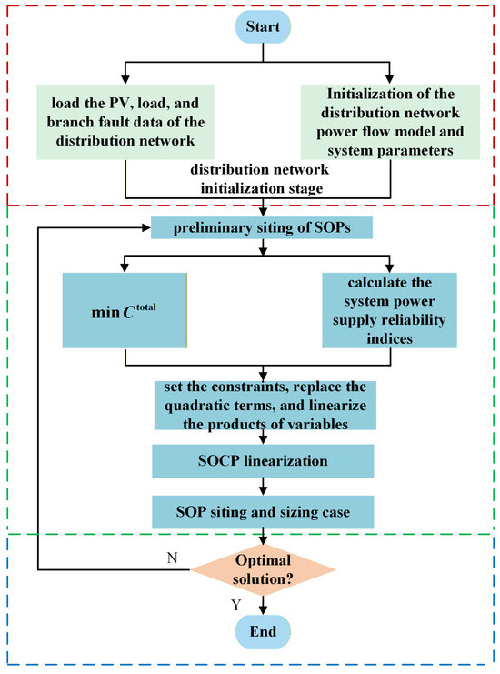
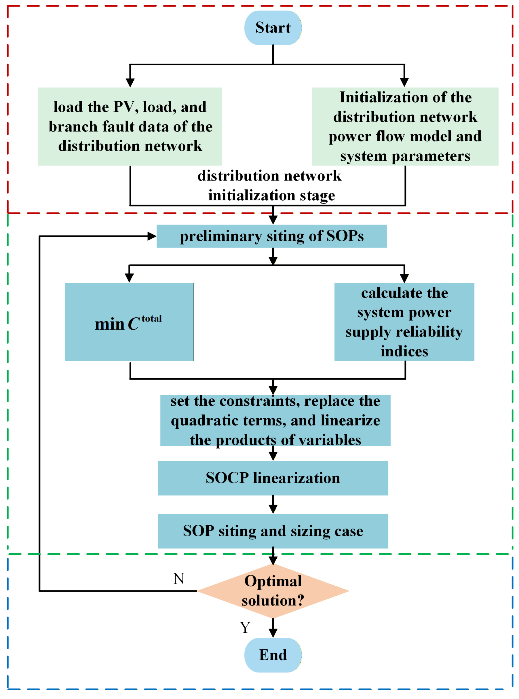
The solution framework for the siting and sizing planning of SOPs is shown in Figure 3. By minimizing the annual comprehensive cost of the distribution network under branch fault conditions as the objective function, the system supply reliability indices are calculated, and the impact of branch faults on different users is analyzed. The specific solution steps are as follows:

Figure 3. Flowchart of the SOP siting and sizing planning process.

(1) First, in the initialization stage of the distribution network, the system parameters are set, and the PV data, load data, and branch fault information of the distribution network are loaded to complete the initialization of the power flow model.

(2) Second, a preliminary siting Case for SOPs is determined by taking the minimization of the annual comprehensive cost of the flexibly interconnected distribution network as the objective function, and the system supply reliability indices are calculated.

(3) Then, the power flow constraints and other constraints of the distribution network are imposed, and the model is linearized by replacing quadratic terms and linearizing the products of variables. The power flow constraints and SOP constraints are transformed into second-order cone constraints and then further linearized, thereby converting the problem into a mixed-integer programming model.

(4) Finally, an optimization solver is used to obtain the configuration Case for the siting and sizing of SOPs. The solution is checked for optimality; if it is not optimal, the siting and sizing of SOPs are updated, and the procedure is repeated. If it is optimal, the loop terminates and the final siting and sizing Case of SOPs, i.e., the optimal solution, is obtained.

4. Case Study

The optimization model was implemented in the GAMS 24.4 environment and solved using the CPLEX solver package. All simulations were performed on a desktop computer equipped with an Intel(R) Core(TM) i7-12700 CPU (2.10 GHz) and 32 GB of RAM, running the Windows 11 operating system. The following subsections present the case study’s system setup and the corresponding numerical results.

4.1. System Setup

In this section, the proposed method is tested on a modified IEEE 33-bus distribution system. The test results are used to verify the effectiveness of SOPs in improving economic performance and reliability indices, as well as the accuracy of the model.

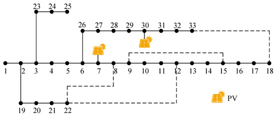
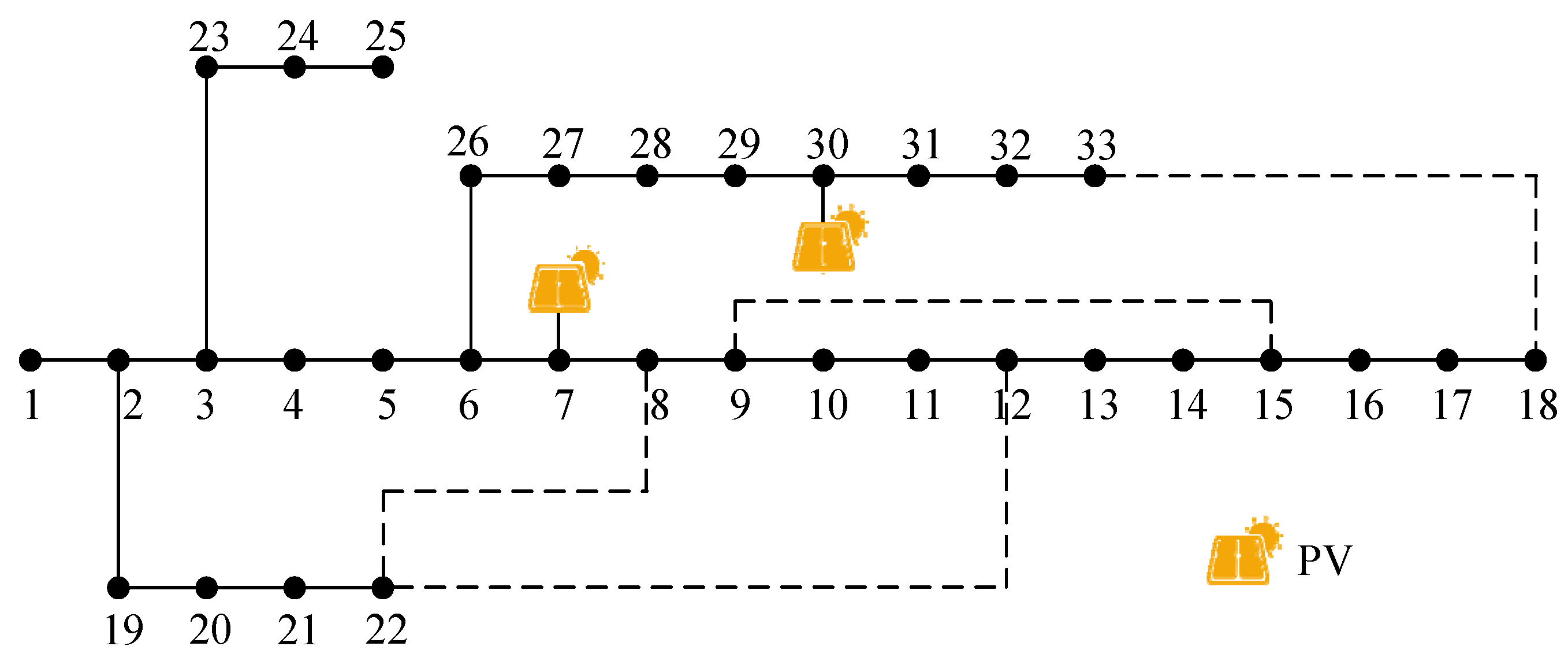
The topology of the system is shown in Figure 4. The system consists of 33 nodes in total, with node 1 being the slack bus. The line segments between nodes 8 and 21, nodes 9 and 15, nodes 12 and 22, and nodes 18 and 33 are considered as candidate locations for SOP installation. The test system contains 32 branches, with a voltage level of 12.66 kV and a base power of 1 MVA. Bus 1 is the slack bus with a voltage of 1.0 p.u., and the maximum and minimum allowable voltage magnitudes are 1.05 p.u. and 0.95 p.u., respectively. The total active and reactive load demands are 3715 kW and 2300 kVar, respectively. The parameters of the distribution network system are given in Table 1.

Figure 4. Modified IEEE 33-bus test case.

Table 1. Distribution network system parameters.

Parameters	Values
$\gamma$	0.02
$r$	0.08
y	20 years
$c^{\mathrm{sop}}$	1000 CNY
$c^{\mathrm{p}}$	20 CNY
$c^{\mathrm{I}}$	1 CNY

Note: All cost data are expressed in Chinese Yuan (CNY). On 15 December 2024, the exchange rate used in this study was 1 USD ≈ 7.28 CNY.

4.2. Analysis of Distribution Network Planning Results

In this paper, two Cases are designed for comparative analysis:

Case 1: the case without SOP planning.

Case 2: the case in which SOPs are installed at candidate locations to restore the power supply to outage areas.

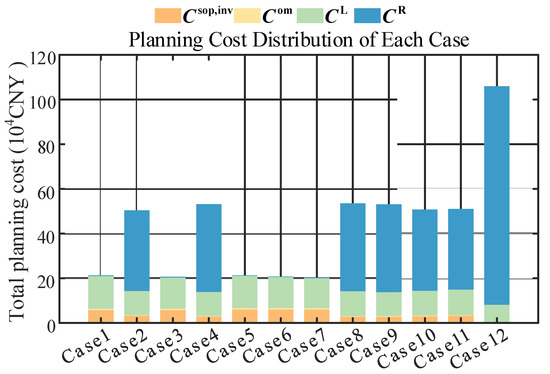
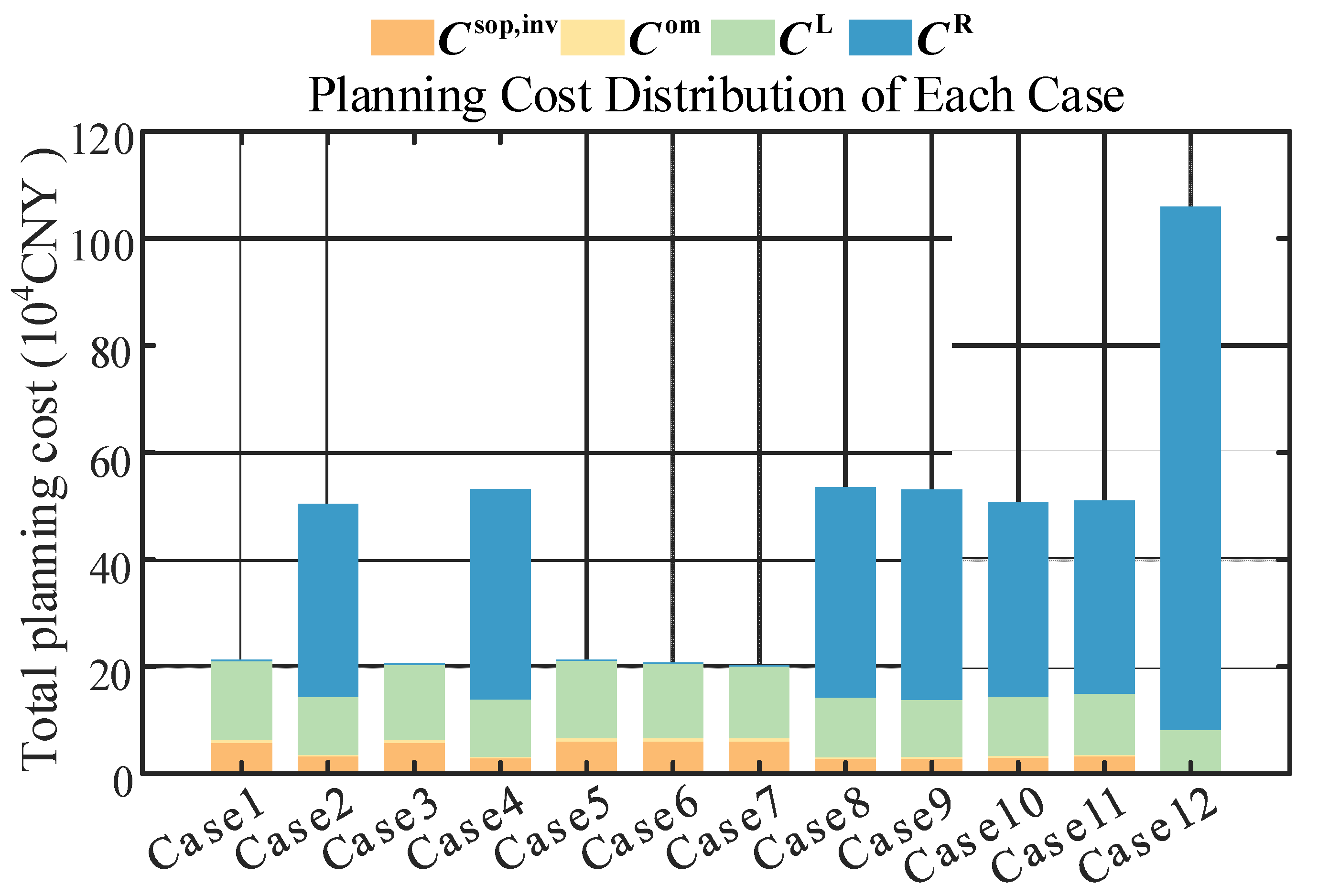
Considering that distributed PV generation will affect the supply restoration of the distribution system, PV units with a capacity of 0.5 MVA are connected at nodes 7 and 30. It is assumed that, in the IEEE 33-bus test system, permanent three-phase faults occur on branches 8–9 and 2–19, causing all loads supplied by nodes 9–18 and 19–22 to be interrupted. By installing SOPs at the candidate locations TS1–TS4 and performing the corresponding analysis and calculations, the planning results for this Case are obtained, as shown in Figure 5. The candidate branches for SOP installation (8–21, 9–15, 12–22, and 18–33) are strategically selected based on their roles as traditional tie-switches and their connectivity to weak terminal nodes in the radial network.

Figure 5. Total planning cost of Example 1.

In Figure 5, the corresponding installation positions of the two-port SOPs are as follows: no SOP installation; 9–15 (TS2), 12–22 (TS1); 8–21 (TS4), 12–22 (TS1); 18–33 (TS3), 8–21 (TS4); 18–33 (TS3), 12–22 (TS1); 8–21 (TS4), 9–15 (TS2); 9–15 (TS2), 18–33 (TS3); 18–33 (TS3); 8–21 (TS4); 9–15 (TS2); 9–15 (TS2), 18–33 (TS3), 8–21 (TS4); and 9–15 (TS2), 12–22 (TS1), 18–33 (TS3). The corresponding calculated costs and reliability indices are shown in Table 2.

Table 2. Calculated costs and reliability indices of Example 1.

SOP Location (kVA)	SOP Cost (104 CNY)	Network Loss (104 CNY)	Outage Cost (104 CNY)	Comprehensive Cost (104 CNY)	Reliability Indices
	$C^{\mathrm{sop},\mathrm{inv}}+C^{\mathrm{om}}$	$C^{\mathrm{L}}$	$C^{\mathrm{R}}$	$C^{\mathrm{total}}$	ASAI
0	0	8.163	97.793	105.956	0.994434
9–15 (0.69), 12–22 (0.248)	10.492	15.815	1.129	27.436	0.999969
8–21 (0.687), 12–22 (0.434)	12.543	15.529	1.391	29.463	0.999966
18–33 (0.479), 8–21 (0.276)	8.445	15.331	0.464	24.24	0.999980
12–22 (0.248), 18–33 (0.712)	10.738	19.308	1.016	31.062	0.999972
8–21 (0.276), 9–15 (0.477)	8.42	14.229	0.465	23.114	0.999980
9–15 (0.34) 18–33 (0.144)	5.423	10.935	36.327	52.685	0.998276
18–33 (0.479)	5.359	12.711	36.392	54.462	0.998272
8–21 (0.276)	3.086	9.241	61.864	74.191	0.996143
9–15 (0.477)	5.334	11.383	36.394	53.111	0.998273
9–15 (0.364), 18–33 (0.121), 8–21 (0.276)	8.511	13.901	0.397	22.809	0.999983
9–15 (0.568), 12–22 (0.272), 18–33 (0.17)	11.295	15.389	0.255	26.939	0.999993

By comparing Case 1 and Case 2 in the table, it can be seen that, compared with the case without SOP planning, the comprehensive cost under line fault conditions is much lower when SOPs are planned. Owing to the voltage support capability of SOPs, the system reliability indices are improved in all cases with SOP installation, indicating that SOPs are highly effective in enhancing supply restoration in distribution networks. In Case 1, where no SOP is planned, the Average Service Availability Index (ASAI) of the system is only 0.994434, which implies that the system is relatively vulnerable under fault conditions. As can be seen from the table, the optimal SOP siting Case is at nodes 9–15, 12–22, and 18–33, with the corresponding SOP capacities of 0.568 MVA, 0.272 MVA, and 0.17 MVA, respectively. Under this Case, the improvement in reliability indices is the most significant, with the ASAI markedly increasing to 0.999993, i.e., from a “two-nine” level to a “five-nine” high-reliability level, approaching an ideal supply state.

Furthermore, after introducing SOP planning (Case 2), although the planning and O&M costs of SOPs amount to 1.1295 × 10⁵ CNY, the self-healing capability of the distribution network is greatly enhanced in terms of post-fault supply restoration. The expected outage loss cost drops sharply from 9.7793 × 10⁵ CNY to 2.55 × 10³ CNY, corresponding to a reduction of 9.7538 × 10⁵ CNY, i.e., a 99.7% decrease. The system’s comprehensive cost is reduced from 1.05956 × 10⁶ CNY to 2.6939 × 10⁵ CNY, a decrease of 7.9017 × 10⁵ CNY, i.e., a 74.6% reduction. At the same time, the reliability indices of the Case with SOPs planned at all three candidate locations are far superior to those of Cases with SOPs planned at only one location, and the outage loads in the distribution network are almost fully restored, while the comprehensive cost is also significantly reduced. Unlike prior works that may encourage over-provisioning for worst-case resilience, our model ensures that the system reliability is enhanced at the minimum comprehensive cost, strictly filtering out economically inefficient capacity expansions. Therefore, the reliability benefits brought by rational SOP planning far outweigh the investment and construction costs of the SOPs themselves. In this study, reliability is monetized through the outage loss cost term, so that investing in SOPs becomes economically justified only when the reduction in outage loss cost compensates the additional investment and O&M costs.

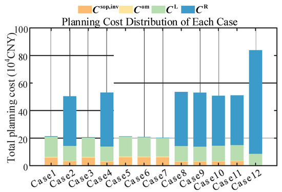
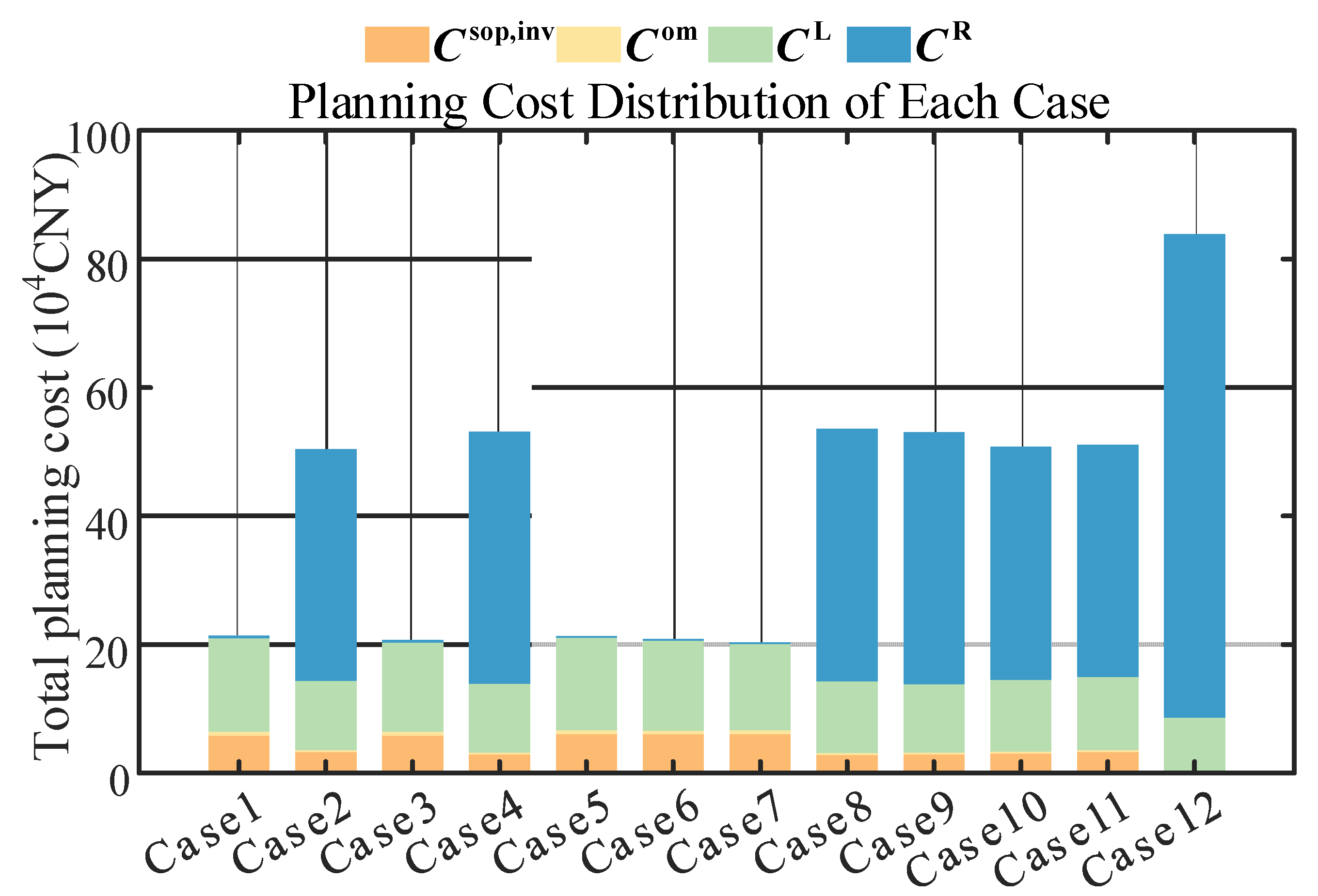
In the IEEE 33-bus test system, similarly, PV units with a capacity of 0.5 MVA are connected at nodes 7 and 30. It is assumed that permanent three-phase faults occur on branches 12–13 and 2–19, causing all loads supplied by nodes 13–18 and 19–22 to be interrupted. By planning SOP devices to restore the power supply, the corresponding comprehensive costs and reliability indices are obtained, as shown in Figure 6.

Figure 6. Total planning cost of Example 2.

In Figure 6, the corresponding installation positions of the two-port SOPs are as follows: no SOP installation; 9–15 (TS2), 12–22 (TS1); 9–15 (TS2), 18–33 (TS3); 9–15 (TS2), 8–21 (TS4); 18–33 (TS3), 12–22 (TS1); 8–21 (TS4), 18–33 (TS3); 12–22 (TS1); 8–21 (TS4); 9–15 (TS2); 18–33 (TS3); and 8–21 (TS4), 9–15 (TS2), 18–33 (TS3). The permissible per-unit voltage range for the restored nodes is set to [0.95, 1.05]. The corresponding calculated comprehensive costs and reliability indices are given in Table 3.

Table 3. Calculated costs and reliability indices of Example 2.

SOP Location (kVA)	SOP Cost (104 CNY)	Network Loss (104 CNY)	Outage Cost (104 CNY)	Comprehensive Cost (104 CNY)	Reliability Indices
	$C^{\mathrm{sop},\mathrm{inv}}+C^{\mathrm{om}}$	$C^{\mathrm{L}}$	$C^{\mathrm{R}}$	$C^{\mathrm{total}}$	ASAI
0	0	8.632	75.225	83.857	0.996145
9–15 (0.298), 12–22 (0.276)	6.422	14.594	0.36	21.376	0.999992
9–15 (0.185), 18–33 (0.134)	3.574	10.743	36.108	50.425	0.998288
9–15 (0.298), 8–21 (0.276)	6.42	13.911	0.36	20.691	0.999991
12–22 (0.276), 18–33 (0.318)	6.645	14.456	0.195	21.296	0.999995
8–21 (0.276), 18–33 (0.318)	8.42	13.944	0.199	20.831	0.999995
12–22 (0.276),	3.088	11.186	39.297	53.571	0.997854
8–21 (0.284)	3.174	2.891	0.284	53.074	0.997856
9–15 (0.298)	3.344	11.156	36.288	50.788	0.998284
18–33 (0.32)	3.577	11.38	36.108	51.065	0.998287
8–21 (0.276), 9–15 (0.173), 18–33 (0.147)	6.659	13.455	0.18	20.294	0.999995

As can be seen from the table, the best performance is obtained when SOPs are sited at nodes 8–21, 9–15, and 18–33, with capacities of 0.276 MW, 0.173 MW, and 0.147 MW, respectively. In this case, the comprehensive cost of the system is reduced by 0.63563 × 10⁶ CNY compared with the scheme without SOP installation, corresponding to a 75.8% decrease. The outage loss cost decreases from 0.75225 × 10⁶ CNY to 0.0018 × 10⁶ CNY, i.e., a reduction of 99.7%. The reliability index ASAI is improved from 0.996145 to 0.999995, achieving a “five-nines” high-reliability supply level. Compared with the case without SOP planning, planning SOPs significantly reduces the comprehensive cost and enhances both the economic performance and the reliability of the distribution system. This study emphasizes the proposed model’s ability to optimize SOP sizing, ensuring that the enhanced reliability is achieved with the highest economic efficiency. By establishing flexible power mutual-support channels, SOPs can effectively improve the operational resilience of the distribution system. It should be noted that the obtained optimal SOP capacity represents the economic equilibrium point. The optimization logic inherently balances the investment cost against the reliability benefits. Any further increase in SOP capacity beyond this point would incur investment costs that outweigh the marginal reduction in outage losses, reflecting the law of diminishing returns in reliability enhancement.

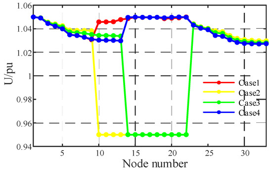
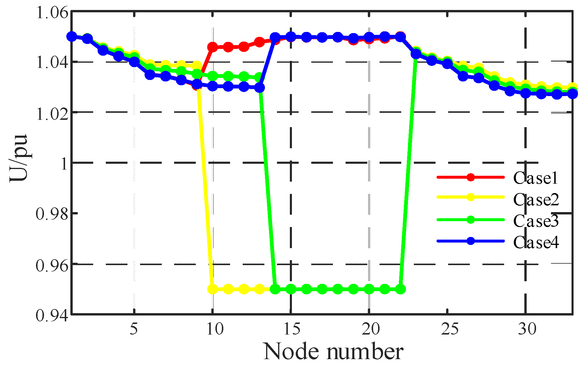
Figure 7 illustrates the nodal voltages in per unit (p.u.) under different SOP siting and sizing schemes. Schemes 1 and 3, and Schemes 2 and 4, respectively, represent the cases with and without SOP planning for the two numerical examples. As shown in the figure, in the open-circuit state without SOP connection, the loads at the faulted nodes are completely interrupted, and their voltages drop to the lower bound of the specified per-unit voltage range, i.e., 0.95 p.u. By contrast, the nodal voltages at buses where SOPs are connected remain relatively stable and are all superior to those in the case without SOP planning. The average voltage deviation is also closely related to the network topology of the system: nodal voltages in p.u. differ among buses, with nodes closer to the power source exhibiting relatively higher voltages, while those at the end of the feeders have lower voltages. This demonstrates that SOPs can improve the voltage profile of the distribution network through power transfer, achieve power flow adjustment, balance the load distribution among feeders, and enhance the supply reliability of the distribution network.

Figure 7. Node voltage (p.u.).

5. Conclusions

To simultaneously address power supply restoration, reliability, and economic performance in distribution networks, this paper proposes a coordinated planning method for flexible distribution networks oriented toward power supply restoration and resilience enhancement. By applying SOPs to the problem of supply restoration in distribution networks, a flexible distribution network planning model is established, which is then solved using second-order cone programming and linearization techniques. Numerical simulations on a modified IEEE 33-bus distribution system lead to the following conclusions:

(1) By reasonably planning the siting and sizing of SOPs, the outage loss cost of the distribution system is significantly reduced, and the comprehensive cost under SOP planning is far lower than that without SOPs, thereby improving the economic performance of the planning case.

(2) With SOP planning, the reliability indices of the distribution system are improved from a “two-nines” level to a “five-nines” high-reliability level. At the same time, SOPs can enhance the reliability of the distribution network by improving the voltage profile through power transfer.

(3) The proposed model is reformulated using a polyhedral approximation method and second-order cone relaxation, which improves the solution efficiency and computational accuracy.

References

- Yuan, Z.; Zhang, H.; Cheng, H.; Liu, L.; Liu, J.; Wang, Y.; Cai, D. Resilience Enhancement of Coordinated Transmission and Distribution System via Risk-based Decentralized Planning Against Typhoons. IEEE Trans. Ind. Appl. 2025, 61, 5780–5796. [Google Scholar] [CrossRef] [Scilit]
- Li, S.; Wang, S.; Zhao, Q.; Liu, D.; Tse, C.K. A risk assessment framework for large-scale synthetic power distribution networks considering historical hurricane disasters. IEEE Trans. Power Syst. 2025, 40, 3846–3858. [Google Scholar] [CrossRef] [Scilit]
- Cao, Y.; Zhou, B.; Chung, C.Y.; Wu, T.; Zheng, L.; Shuai, Z. A coordinated emergency response Case for electricity and watershed networks considering spatio-temporal heterogeneity and volatility of rainstorm disasters. IEEE Trans. Smart Grid 2024, 15, 3528–3541. [Google Scholar] [CrossRef] [Scilit]
- Sun, S.; Li, G.; Bie, Z.; Dong, Z.Y.; Liu, J.; Chen, M.; Li, F.; Xu, M. Resilience Assessment of Power Distribution System against Rainstorm-Induced Urban Waterlogging. IEEE Trans. Ind. Appl. 2025, 61, 7916–7928. [Google Scholar] [CrossRef] [Scilit]
- Gao, H.; Guo, M.; Liu, J.; He, S.J. Power Supply Challenges and Prospects in New Power System from Sichuan Electricity Curtailment Events Caused by High-temperature Drought Weather. Proc. CSEE 2023, 43, 4517–4538. [Google Scholar] [CrossRef]
- Zhao, S.; Wang, J.; Hu, W.; Cao, D. Resilience Assessment of Distribution Networks Considering EV Charging Loads under Extreme Heat. In Proceedings of the 2025 8th International Conference on Electrical Engineering and Green Energy (CEEGE), Yangzhou, China, 4–6 July 2025; IEEE: New York, NY, USA, 2025; pp. 77–81. [Google Scholar] [CrossRef] [Scilit]
- Hou, G.; Muraleetharan, K.K.; Panchalogaranjan, V.; Moses, P.; Javid, A.; Al-Dakheeli, H.; Bulut, R.; Campos, R.; Harvey, P.S.; Miller, G.; et al. Resilience assessment and enhancement evaluation of power distribution systems subjected to ice storms. Reliab. Eng. Syst. Saf. 2023, 230, 108964. [Google Scholar] [CrossRef] [Scilit]
- Räisänen, O.; Saleem, A.; Lehtonen, I.; Haakana, J.; Haapaniemi, J.; Lassila, J. High-resolution model for assessing the impact of climate change on the outage risk caused by crown snow load in distribution networks. Reliab. Eng. Syst. Saf. 2025, 267, 111864. [Google Scholar] [CrossRef] [Scilit]
- Kang, C.; Yap, L. Key scientific issues and theoretical research framework for power systems with high proportion of renewable energy. Autom. Electr. Power Syst. 2017, 41, 2–11. [Google Scholar] [CrossRef]
- Xie, L.; Li, Y.; Luo, L.; Zeng, X.; Cao, Y. A vulnerable points identification method based on complex network theory and an operation index. Power Syst. Prot. Control 2022, 50, 83–91. [Google Scholar] [CrossRef]
- Song, Y.; Sun, C.; Li, P.; Yuan, K.; Song, G.; Wang, C. SOP based supply restoration method of active distribution networks using soft open point. Proc. CSEE 2018, 38, 4390–4398. [Google Scholar] [CrossRef]
- Wang, Y.; Ma, J.; Wang, X.; Xu, Y.; He, J.; Li, J. Critical Load Restoration Method for Distribution Network with Soft Open Point. Autom. Electr. Power Syst. 2021, 45, 104–111. [Google Scholar] [CrossRef]
- Yang, M.; Zhang, S.; Cheng, H.; Zheng, S.; Liu, J.; Cao, Y.; Xiao, T.; Liang, Y. Reliability Assessment for SOP-based Flexible Interconnected Distribution Network Considering Post-fault Multi-stage Recovery. Proc. CSEE 2024. Available online: https://link.cnki.net/urlid/11.2107.tm.20240914.1110.008 (accessed on 21 December 2025).
- Fan, P.; Yu, T.; Wang, Z.; Xiao, W.; Pan, Z. Optimal deployment of Multi-type Switches in Flexible Distribution Network by Explicitly Integrating Reliability Expressions. Proc. CSEE 2024. [Google Scholar] [CrossRef]
- Pamshetti, V.B.; Singh, S.; Thakur, A.K.; Singh, S.P.; Babu, T.S.; Patnaik, N.; Krishna, G.H. Cooperative operational planning model for distributed energy resources with soft open point in active distribution network. IEEE Trans. Ind. Appl. 2023, 59, 2140–2151. [Google Scholar] [CrossRef] [Scilit]
- Xiao, J.; Li, Y.; Han, Y.; Qiao, X.; Zhong, J. Resilience Enhancement Strategy for Distribution Networks Considering the Spatiotemporal Characteristics of Typhoon and the Coordinated Optimization of Flexible Resources. Trans. China Electrotech. Soc. 2024, 39, 7430–7446. [Google Scholar] [CrossRef]
- Zhao, J.; Chen, H.; Song, G.; Fan, X.; Li, P.; Wu, J. Planning method of soft open point in distribution network considering reliability benefits. Autom. Electr. Power Syst. 2020, 44, 22–31. [Google Scholar]
- Li, P.; Ji, J.; Ji, H.; Song, G.; Wang, C.; Wu, J. Self-healing oriented supply restoration method based on the coordination of multiple SOPs in active distribution networks. Energy 2020, 195, 116968. [Google Scholar] [CrossRef] [Scilit]
- Sun, S.; Wei, C.; Qiu, J. Distributed power restoration method for smart distribution network with soft open point. Autom. Electr. Power Syst. 2022, 46, 79–85. Available online: https://link.cnki.net/urlid/32.1180.TP.20211126.1339.004 (accessed on 21 December 2025).
- Ge, S.; Yang, Z.; Liu, H.; Wang, C.; Zhao, L.; Liu, S. Reliability and Power Supply Capability Evaluation of Active DistributionNetworks with Four-terminal Soft Open Points. High Volt. Eng. 2020, 46, 1124–1136. [Google Scholar] [CrossRef]
- Jiang, X.; Zhou, Y.; Ming, W.; Yang, P.; Wu, J. An overview of soft open points in electricity distribution networks. IEEE Trans. Smart Grid 2022, 13, 1899–1910. [Google Scholar] [CrossRef] [Scilit]
- Zhang, B.; Liu, S.Y.; Lin, Z.Z.; Yang, L.; Gao, Q.; Xu, H. Distribution network reconfiguration with High Penetration of Renewable Energy Considering Demand Response and Soft Open Point. Power Syst. Autom. 2021, 45, 86–94. Available online: https://link.cnki.net/urlid/32.1180.TP.20200515.1111.002 (accessed on 21 December 2025).
- Xiao, J.X.; Li, Y.; Qiao, X.B.; Tan, Y.; Cao, Y.; Jiang, L. Enhancing hosting capacity of uncertain and correlated wind power in distribution network with ANM strategies. IEEE Access 2020, 8, 189115–189128. [Google Scholar] [CrossRef] [Scilit]
- Ling, F.; Zhu, J.; Sheng, W.; Zhang, D.; Liu, K.; Li, Y.; Liu, J.; Tang, H. Source-Network-Storage Coordinated Planning for Multi-Region Flexible Interconnected Distribution System Based on Distributed Optimization. Electr. Power Autom. Equip. 2025, 45, 62–69. [Google Scholar] [CrossRef]
Disclaimer/Publisher’s Note: The statements, opinions and data contained in all publications are solely those of the individual author(s) and contributor(s) and not of MDPI and/or the editor(s). MDPI and/or the editor(s) disclaim responsibility for any injury to people or property resulting from any ideas, methods, instructions or products referred to in the content. |
© 2026 by the authors. Licensee MDPI, Basel, Switzerland. This article is an open access article distributed under the terms and conditions of the Creative Commons Attribution (CC BY) license.