


Abstract
Accurate prediction of the rocking and sliding response of free-standing rigid blocks under seismic excitation remains challenging, particularly in regimes where rocking and sliding are strongly coupled and motion mode transitions occur. This study presents a modified semi-analytical framework and an optimized Finite Element Method (FEM) approach to investigate the nonlinear dynamics of rigid rectangular blocks subjected to initial angular displacements, assuming Coulomb friction and near-inelastic impacts. The proposed semi-analytical formulation explicitly captures the coupling between rocking and sliding motions, enabling systematic identification of rest, rocking, sliding, rocking–sliding, and free-flight response modes. Benchmark comparisons with Veeraraghavan’s classical model show overall agreement in limiting cases but reveal notable differences in intermediate regimes, where motion mode transitions are highly sensitive to friction coefficient and slenderness ratio. These discrepancies arise from the ability of the present formulation to resolve transitional rocking–sliding behavior that is not fully represented in uncoupled or limiting-case assumptions. Complementary FEM simulations employing both rigid and deformable body representations further elucidate the role of contact modeling and energy dissipation. While rigid-body FEM models offer computational efficiency, they exhibit localized penetration and residual bouncing due to contact enforcement limitations. In contrast, deformable FEM models more closely approximate near-inelastic collision behavior and dissipate impact energy more effectively, albeit at higher computational cost. The combined semi-analytical and FEM results provide a robust framework for interpreting motion mode transitions, quantifying contact and penetration effects, and defining the applicability limits of simplified rigid-body models. These findings offer practical guidance for selecting appropriate modeling strategies for seismic response assessment of free-standing rigid blocks.
1. Introduction
In the realm of earthquake engineering, the behavior of free-standing objects, especially in the context of rocking and sliding, has been a topic of lasting interest. The study of the dynamic response of rigid blocks, especially under external excitations such as earthquakes, has garnered significant attention within the earthquake engineering community [1,2,3,4,5,6,7]. This interest has been sustained, in part, due to the idealization of rigid blocks undergoing negligible deformation as rigid bodies, which offers an avenue for more straightforward analytical solutions [8,9,10,11]. This simplification is especially valuable in scenarios ranging from engineering applications to computer graphics and robotics. Traditional studies have primarily considered these bodies in a two-dimensional plane, focusing exclusively on planar rocking [12,13,14,15,16,17,18,19]. However, real-world scenarios often involve bi-directional earthquake excitations, rendering the planar assumption insufficient. This is especially true when the friction coefficient is not particularly high. Recognizing this research gap, recent studies have ventured into three-dimensional models of these rigid blocks, aiming to capture the intricacies of their movement more accurately [12,20]. These models, validated against both other numerical predictions and real-world shake table tests, have shown promising results, emphasizing the necessity for a more comprehensive modeling approach. As the field moves forward, the focus shifts towards creating optimized solutions and tools for predicting the dynamic behaviors of these rigid bodies under various conditions. While many experts have worked on this topic, only few were able to extend the knowledge base on these rigid-block dynamics [1,3,8,14,21,22,23,24,25,26,27,28], leverage previous findings, and provide a comprehensive understanding of the subject [12,16,18,19,29]. In earlier research, most investigations concentrated primarily on the fundamental rocking and sliding responses of these blocks [15,18,30,31,32].
Recent studies have advanced the understanding of rocking and overturning dynamics in rigid-block systems across a broad range of seismic applications. Early research examined collision behavior and restitution effects between interconnected rigid bodies [33], followed by the development of energetic restitution-based models for rocking under base excitation [17]. Three-dimensional extensions in the study of rocking dynamics revealed how variations in geometric and inertial properties significantly affect the stability of free-standing blocks [18], while related investigations quantified overturning risks for furniture and other nonstructural components subjected to earthquake loading [34]. Response mitigation has also been addressed, with tuned mass absorbers shown to significantly reduce the rocking amplitudes and overturning tendencies of rigid blocks [35]. Additional contributions examined rocking under specialized loading environments, including cycloidal seismic pulses and pulse-type ground motions for both free-standing and anchored blocks [29,36]. The uplift and overturning mechanisms of anchored equipment have been further characterized to clarify stability limits under strong shaking [37], while the rocking spectrum framework has highlighted important limitations of prevailing design methodologies and underscored the need for more robust predictive models for rocking-dominated systems [38].
These studies have shown the necessity of understanding block motions in both two-dimensional and, importantly, three-dimensional contexts [39,40,41,42,43]. In particular, while two-dimensional analyses are informative, they often miss the complexities inherent in real-world three-dimensional systems. Recent advances have highlighted the significance of three-dimensional analyses, especially when assessing seismic risks [31,42]. Algorithms and methodologies have been developed to address the challenges posed by these analyses, from handling complex surface-to-surface impacts to dealing with possible sticking and slipping motions during impacts [22,44,45,46]. According to earlier research by Scalia and Sumbatyan [21], they found that slide rotation cannot occur when the friction coefficient is very small ( ≪ 1). Scalia and Sumbatyan discovered the “jump” phenomena only when the friction level is very high and occurs precisely at the moment the block reaches its overturning angle . This was carried out based on numerical evaluation of a nonlinear differential equation governing the rotational function . Several researchers have used finite element modeling (FEM) has been applied to investigate the rocking response of rigid blocks. Ohshima et al. [47] conducted a 2D study, and Wolf [48,49,50,51] investigated the problem of base mat elevation using a 3D finite element model. Despite an increase in overall displacements, they discovered that stress effects decreased with elevation. Despite the fact that it allows for more realistic modeling, FEM costs a significant amount of computational time.
Advanced data-driven numerical approaches have been increasingly explored for predicting seismic response. Bhatta et al. [52] demonstrated the use of machine learning techniques for estimating seismic damage in reinforced concrete buildings, highlighting the potential of such methods for large-scale structural performance assessment. Similarly, recent work published in Applied Sciences [53] examined nonlinear dynamic response characteristics under seismic excitation, emphasizing the importance of detailed numerical modeling in capturing complex response behaviors. Although these contributions primarily address the seismic response at the structural-system level, the present study focuses on the fundamental mechanics governing the behavior of rigid free-standing blocks. In particular, attention is given to rocking–sliding coupling, impact-induced pivot switching, and contact-related nonlinearities. The proposed modified semi-analytical and FEM-based framework is therefore complementary to existing system-level and data-driven approaches, offering a physically grounded basis for interpreting motion-mode transitions and contact effects under seismic excitation.
This study aims to predict the response modes of free-standing rigid blocks under seismic excitation employing modified semi-analytical methods and optimized FEM techniques. Unlike previous studies, the developed models incorporate all geometric nonlinear effects as well as potential sliding, uplift, bouncing, or free flight; and the penetration of the rigid block into a pedestal without omitting any terms in the dynamic equations of motion. The models describe the rigid body’s motion by tracking the time histories of the center-of-mass displacements, rotation, and sliding of the block. This study further compares and assesses the performance of the modified analytical techniques and optimized FEM when simulating rigid-block response modes with the research of Veeraraghavan et al. [20]. Additionally, we aim to identify the strengths and limitations of each approach and provide useful insights for engineers and researchers engaged in the analysis and design of rigid-block structures by performing a thorough numerical investigation.
The structure of this study is organized into several sections, each serving a specific purpose in achieving the research objective of comparing and evaluating the performance of the analytical approach and the FEM in simulating the dynamic behaviors exhibited by rigid blocks.
Section 2 reviews the modified semi-analytical procedure and the computational algorithm applied to evaluate the dynamic behavior of rigid blocks. Section 3 introduces the optimized FEM numerical technique for simulating the response modes of rigid blocks. Section 3 introduces the optimized FEM numerical technique for simulating the response modes of rigid blocks. In Section 4, research focuses on validating the modified semi-analytical and FEM approaches. It describes the methodology used to compare and evaluate the performance of both methods and discusses the obtained results, including the displacements and rocking and sliding in comparison with the accuracy and reliability of each approach. Lastly, Section 5 summarizes the key findings and implications of our research.
2. Modified Semi-Analytical Nonlinear Formulation
In this study, the system illustrated in Figure 1, is used, where rocking motion occurs about the rotation points and . The block’s mass center is located at its geometric midpoint, positioned a distance R from each corner. Based on the applied ground acceleration and the friction coefficient , the block may move with the ground, begin to rock, or transition into sliding. The block will engage in rocking only if the condition is satisfied [21,26,29]. Prior studies have also examined circumstances under which sliding may occur concurrently with rocking by the authors of [12,13,14,23,27,41,44,45,46,54]. Zhang & Makris [29]’s study is otherwise called the semi-analytical method, as their developed linear formulation was intended to avoid sliding with the condition that the ratio of the horizontal to vertical reaction must be less than the coefficient of friction.
Figure 1.
Modes of response of a free-standing rigid block subjected to dynamic excitation. (a) Rest and sliding modes, where motion is dominated by horizontal translation and frictional resistance. (b) Rotation and slide–rotation modes: in the rotation mode, the block undergoes pure rocking about corner or with no relative slip at the contact interface (), whereas in the slide–rotation mode, rocking is accompanied by simultaneous horizontal sliding once the friction force reaches the Coulomb limit ().
In this study, we have modified Zhang & Makris’s [29] equations in the sense that the frictional force may not be sufficient, which invariably introduces the possibility of sliding. Whenever there is sliding, the model changes from a single degree of freedom to two degrees of freedom. Zhang & Makris proposed that sliding would not occur provided the friction between the block and its support surface is sufficiently high throughout the rocking motion.
When subjected to a positive horizontal base acceleration , the block first rotates in the negative direction, , and if an overturning does not take place, its motion alternates between negative and positive rotations. By considering the vertical base acceleration to be zero (), the governing equations for a free-standing block of mass m become:
and
Here, denotes a parameter with units of rad/s, and represents the signum function. As the block size increases (i.e., as R becomes larger), the value of p decreases accordingly. The natural frequency of a rigid block in free vibration is not constant, as it depends on the vibration amplitude [1]. Nevertheless, the parameter p effectively characterizes the dynamic behavior of the system. During rocking, the motion is assumed to transition continuously as the rotation axis shifts from to . By applying angular momentum conservation about point immediately before and after impact, the relationship between (the pre-impact angular velocity) and (the post-impact angular velocity) is obtained. The ratio of kinetic energy after and before the impact is as follows:
The angular velocity immediately following impact is twice the angular velocity just prior to the impact. By substituting Equation (5) into Equation (4) the corresponding expression for the coefficient of restitution is obtained. Equation (6), provides the upper bound of the restitution coefficient r for which a slender block will still experience rocking motion. If further energy dissipation occurs through interface mechanisms, the actual restitution coefficient r will be smaller than the value predicted by Equation (6). In this work, the analysis is performed using the maximum restitution coefficient specified in Equation (6).
Equations (1) and (2) are widely recognized in the literature (e.g., [3,24,25,29]). These equations remain applicable for any value of the block angle . For tall, slender blocks, the angle becomes small, allowing Equations (1) and (2) to be linearized. Closed-form solutions to the linearized system under harmonic excitation have been provided by Housner [1] for positive rotations only () and by Hogan [25] for positive and negative rotations. Here, the linearized equations are solved for free vibration in both positive and negative directions to revisit overturning conditions associated with Housner’s half-sine pulse [1] and to examine the rocking response of rigid blocks subjected to cycloidal pulses. Within the limits of the linear approximation and for a harmonic ground acceleration with amplitude and angular frequency , we have the following:
2.1. Nonlinear Equations of Motion of a Planar Double Pendulum
We consider a planar double pendulum composed of two rigid, massless links of lengths and , carrying point masses and at their distal ends in Figure 2. The motion is confined to a vertical plane under uniform gravity g. Generalized coordinates are chosen as the absolute angles and of the first and second links, respectively, measured from the downward vertical. For compactness, we introduce the angle difference
and the weight parameters
Figure 2.
Planar double pendulum used as a conceptual model for the nonlinear equations of motion. The rigid, massless links of lengths and carry point masses and , respectively. Angles and are measured from the vertical, and gravity g acts in the negative Z–direction, consistent with the global X–Z coordinate system.
2.1.1. Kinematics
With the fixed hinge at the origin, the Cartesian coordinates of the two masses are as follows:
Differentiation with respect to time provides the velocities. For the first mass,
while for the second mass,
2.1.2. Lagrangian Formulation
The kinetic and potential energies of the system are as follows:
The Lagrangian is . Using the Euler–Lagrange equations
and carrying out simplification, one obtains the coupled nonlinear equations of motion:
2.1.3. Second-Order Matrix Form
Define the generalized coordinate vector:
2.1.4. First-Order Form for Time Integration
For numerical time integration, it is convenient to express the system as a first-order set of differential equations. We introduce the following state vector:
and the kinematic relations imply
Equations (24) and (25) can be assembled together with the kinematic relations into a compact form:
with the “mass” matrix
and the right-hand-side vector
System (26) is directly suitable for implicit ODE solvers that accept a configuration-dependent mass matrix, such as ode15s in MATLAB (R2023a).
2.2. Condition for Sustaining Rocking and Sliding Motion
When the block is rocking, the horizontal and vertical reactions at points or fluctuate with time, and the dynamic equilibrium in the horizontal and vertical directions produces Equations (29) and (30):
From Figure 1, is positive to the right, and is positive in the upward direction. Considering the free-body diagram in Figure 1, the vertical reaction consists of two forces, which are the gravitational force (i.e., weight of the block) and vertical inertia force. Similarly, in the horizontal direction, the horizontal reaction consists of two forces, which are the horizontal inertia force and the frictional force that the block is experiencing at the contact point. As illustrated in Figure 1b, the distinction between the rotation and slide- rotation modes lies in the contact condition at the base: the rotation mode corresponds to sticking contact with pure rocking about a pivot corner, while the slide–rotation mode involves simultaneous rocking and horizontal slip once the frictional resistance reaches its limiting value.
To provide a unified visual summary of the physical mechanisms, response regimes, and transition events considered in the proposed rocking–sliding framework, Figure 3 presents a schematic overview encompassing contact forces, frictional constraints, impact-induced pivot switching, and loss-of-contact conditions.
Figure 3.
Schematic overview of the modeled physical mechanisms and response regime transitions for a free-standing rigid block. The arrows indicate admissible transitions between response regimes, with colors and line styles corresponding to the physical and numerical mechanisms summarized in the legend. The diagram summarizes (a) the block geometry and degrees of freedom, including rocking rotation and horizontal sliding , contact reactions and governed by Coulomb friction (), and geometric parameters b, h, , and measured from the vertical; and (b) the admissible response regimes and transitions, including pure rocking, rocking–sliding, impact/collision with pivot switching between corners and when , and loss-of-contact (free flight) when . The schematic also indicates numerical contact artifacts observed in FEM simulations, such as minor penetration and small rebound amplitude arising from penalty-based contact enforcement under near-inelastic impact conditions.
We assume in Equation (29) since there is no ground acceleration in our case but rather an initial displacement of the block, where and are the horizontal and vertical displacements (the inertial forces in the horizontal and vertical direction) of the center of mass of the block. The kinematics of the rocking motion yields the following:
where = the angular velocity of the block, and = the angular acceleration of the block that is given by Equation (31); moreover, (19) can also be found in the study by Pompei [23]. By substituting Equations (29) and (30) into Equation (9) together with Equations (31) and (32), the resulting expression provides the criterion required to prevent sliding throughout the rocking motion. The condition that ensures sliding does not occur during the full rocking response is expressed as follows:
Although the present simulations focus on short-duration responses under initial angular displacement to isolate fundamental rocking, sliding, and impact mechanisms, the governing equations explicitly retain the base acceleration term and can therefore be directly extended to longer time histories and arbitrary time-varying excitations, including recorded earthquake ground motions.
It can be readily confirmed that, under a one-sine pulse at the instant when rocking begins at , the initial conditions satisfy and . With these initial conditions, Equation (33) simplifies to Equation (8), , which corresponds to the classical expression obtained from static analysis.
For this study, we have to account for sliding by adding another degree of freedom. Figure 1 only has one degree of freedom, which is the angle of rotation , and it needs to be modified to include sliding. The sliding movement in the horizontal direction is considered to be in the opposite direction of the rocking angle , which is positive. The frictional force is always present as long as the block is in contact with the ground surface. Therefore, whenever the inertia force exceeds the frictional force, the block tends to slide due to insufficient frictional force.
Given that the gravitational acceleration is and the half-diagonal length of the block is (which serves as a geometric indicator of the block’s size), represents the frequency characteristics of the block. Assuming that the block–ground interaction is perfectly inelastic, such that the restitution coefficient satisfies . Following impact with the ground, the reduction factor applied to the block’s angular velocity is given by by Kimura et al. [55].
When the block enters its free-vibration regime, we have (time of impact) and . The time of excitation is given by , with the condition that as long as , . If , then the case becomes a forced vibration, and .
Similarly to Zhang & Makris [29], a numerical integration is performed using the built-in Ordinary Differential Equation (ODE) solvers available in MATLAB (R2023a). A state-space representation is constructed to capture the nonlinear dynamics associated with both rocking and sliding of the block. The system state is expressed in vector form as:
and the corresponding time-derivative vector is given by
For slender blocks, the linearized form provides an accurate approximation, and Equation (35) simplifies to:
The equation now becomes four-dimensional instead of two-dimensional, which was originally presented by Zhang & Makris [29] due to the addition of the sliding displacement and velocity. Subtracting the frictional force from the inertial force produces the required force needed for the block to slide. In order to account for the mass matrix in Equations (29) and (30), the mass variable is implemented in the ODE solver to obtain the mass function, along with a function that detects impact whenever the angle of rotation is zero. We also keep track of which corner of the block (corner and ) is experiencing rocking, along with the impact times and instances when the mode changes without impact.
During coupled rocking–sliding motion, the governing equations can be expressed in a configuration-dependent mass-matrix form. In particular, the off-diagonal inertia term represents the coupling between the horizontal translational velocity and the angular acceleration of the block while in contact with the ground. By considering the kinematics of the block’s center of mass relative to the active pivot corner, the horizontal inertial contribution associated with angular motion yields
where m is the block mass, is the half-diagonal length, is the slenderness angle, and is the instantaneous rocking rotation. This term physically represents the inertia-induced coupling between horizontal sliding and rotational motion during rocking. The mass-matrix entry is updated dynamically at each time step during ground contact and is set to zero upon loss of contact, ensuring correct momentum transfer and force equilibrium throughout rocking–sliding transitions.
The complete numerical procedure used to simulate coupled rocking and sliding, including impact detection and state switching, is summarized in Algorithm 1.
| Algorithm 1 Rocking and Sliding Block Simulation |
|
2.3. Numerical Implementation and Solver Selection
Time integration of the governing equations is performed using MATLAB’s variable-step Runge–Kutta solver ode45 combined with event detection to capture impact instants. Although discontinuities arise at impacts, the equations of motion remain non-stiff between events, rendering ode45 both accurate and computationally efficient for the present formulation. The numerical tolerances were fixed at and for all simulations.
To verify numerical robustness, selected cases were re-simulated using the stiff solver ode15s with identical tolerance settings. The resulting differences in peak rocking angle and sliding displacement were consistently below across all tested parameter sets, confirming that stiffness effects are confined to discrete impact instants and that the chosen solver does not influence the predicted motion modes.
Table 1 demonstrates that both solvers yield nearly identical peak rocking and sliding responses, with relative differences below 1.1%. However, ode45 requires substantially fewer time steps and function evaluations, resulting in a runtime reduction of approximately 70% compared to ode15s. Given that stiffness is localized primarily at impact instants, ode45 is adopted for all parametric simulations.
Table 1.
Comparison of MATLAB ODE solvers used for rocking–sliding simulations (representative case: , , ).
3. FEM Simulation of Rocking and Sliding Response of Free-Standing Rigid Blocks
This section examines how a single rigid-block system responds to rocking and sliding motions when analyzed through FEM. A numerical investigation was carried out to study the interaction between a free-standing rigid block and an infinitely massive pedestal, accounting for both static and kinetic frictional effects. With this model, we studied the the impact behavior of a two-dimensional rectangular block. In this analysis, a rigid-block model presented in Figure 4 characterized by a half-height of , half-width of , with a block mass of taken into account, and it is in contact with the ground at corners and .
Figure 4.
Finite element idealization and kinematic configurations of a free-standing rigid block. (a) Geometry of a rectangular block in height , width , and mass m, resting on a rigid pedestal with contact at corners and . The global axes and gravity g are also indicated. (b) Discrete rigid block and analytical rigid pedestal, showing contact points and and reference nodes at the centroid, boundary conditions, and gravity. The initial tilted configuration used in the simulations, defined by angle and the prescribed translational and rotational velocities at the center of mass.
As mentioned above, all parts were modeled as a collection of rigid bodies. A rigid body consists of nodes, elements, or surfaces whose movement is controlled through a designated reference node, known as the rigid-body node. The spatial relationships among its nodes and elements are preserved during the simulation. Therefore, the constituent elements do not deform but can undergo large rigid-body motions. In this model, the mass and inertia are assigned. The moment of rotational inertia is calculated according to Equation (38).
The motion of each rigid body is defined by imposing boundary conditions at its reference node, which is positioned at the centroid of the body. All rotations and displacements are restricted in the pedestal, and an acceleration of gravity of 9.81 m/s2 in the negative direction of Y is considered. In this analysis, following the approach of Veeraraghavan et al. [20], the friction coefficient is specified as , and the initial conditions include a translational velocity of together with a rotational velocity of . Veeraraghavan assumed a perfectly inelastic block–ground interaction with a restitution coefficient of , although ABAQUS does not incorporate a restitution parameter; thus, our study proceeds using the discrete rigid-body modeling approach.
The block was defined as discrete rigid parts for which their mesh is composed of a two-node 2D linear rigid link in plane stress (R2D2 according to ABAQUS/Standard 2022 nomenclature [56]). A discrete rigid part resembles a deformable part in the sense that it may possess any arbitrary geometry. However, it is treated as perfectly rigid and is employed in contact simulations to represent bodies that do not undergo deformation. Being a 2D rigid body, it is only necessary to mesh the boundaries. On the other hand, the pedestal is defined as an analytical rigid part, and these types of parts are not discretized.
3.1. Mesh Convergence Analysis of the Rigid-Body FEM Model
Although the rigid block is modeled as a discrete rigid body using R2D2 elements, the spatial discretization of its boundary can still influence contact mechanics, particularly penetration depth and contact force transmission at the block–pedestal interface. To ensure numerical robustness and mesh-independent results, a mesh convergence study was conducted.
The rigid block boundary was discretized using three different mesh densities: a coarse mesh (4 R2D2 elements per edge), a medium mesh (8 R2D2 elements per edge), and a fine mesh (16 R2D2 elements per edge). All other model parameters, including mass properties, contact formulation, friction coefficient, damping parameters, and time integration settings, were held constant. Convergence was assessed by monitoring (i) the peak horizontal displacement of the block’s center of mass, (ii) the peak angular velocity during rocking, and (iii) the maximum penetration depth observed at the contact corners. These quantities are directly related to motion mode prediction and contact accuracy.
The results indicate that increasing the mesh density from the coarse to the medium discretization leads to noticeable reductions in penetration depth and improved smoothness in contact force transmission. However, further refinement from the medium to the fine mesh results in changes of less than 1% in peak displacement and angular velocity, and negligible variation in penetration depth. This confirms that the solution has effectively converged with respect to mesh density. Based on these observations, the medium mesh discretization was adopted for all subsequent simulations, as it provides a reliable balance between numerical accuracy and computational efficiency while minimizing mesh-induced artifacts. The quantitative convergence results for peak displacement, angular velocity, and maximum penetration depth under different mesh densities are summarized in Table 2. As shown in Table 2, variations in peak displacement and angular velocity between the medium and fine meshes remain below 1%, confirming mesh-independent rigid-body response.
Table 2.
Mesh convergence study for the rigid-body FEM model discretized with R2D2 elements.
This study employs an explicit dynamic analysis procedure. Within an explicit framework, the nodal accelerations are determined directly without iterative correction by multiplying the inverse of the diagonal mass matrix with the resultant nodal force vector. This resultant force incorporates contributions from external actions (such as body loads, surface pressures, and contact interactions), element stresses, damping effects, bulk viscosity, and hourglass-control mechanisms. Once the accelerations at time n are obtained, the velocities are updated to time , and the corresponding displacements are computed at time . Strains follow from the updated displacements, and stresses follow from the strains, completing a cycle that repeats at each time increment. In this work, an explicit formulation is chosen rather than an implicit one, as it is more suitable for advancing the solution over very small time steps and offers significantly lower computational cost.
The essential distinction between explicit and implicit approaches arises from the numerical strategy used to evaluate derivative terms. In static analyses, inertial and damping effects are absent, whereas dynamic analyses incorporate forces associated with inertia and damping. ABAQUS/Standard utilizes an implicit solver for static simulations, while dynamic simulations may be performed using either the explicit or implicit formulation available within ABAQUS/Explicit.
In nonlinear implicit analysis, each load or time step requires multiple iterations of trials to achieve equilibrium within a specified tolerance. In contrast, explicit analysis avoids iterative procedures because the accelerations are evaluated directly. The stability of explicit integration imposes a restriction on the time increment, which must remain below a critical value related to the smallest characteristic element length, essentially the time required for a stress wave to traverse an element. Consequently, there is a strong emphasis on mesh refinement to identify the smallest element that governs the stable time increment. Implicit transient analysis, however, is not limited by such a condition and typically permits time increments several orders of magnitude larger than those used in explicit analysis.
Implicit methods require the repeated inversion of the stiffness matrix, often one or more times per load or time step, which can become computationally expensive for large-scale models. Explicit methods circumvent this cost entirely. Furthermore, explicit solvers manage nonlinearities including contact and material nonlinear behaviors, with relative simplicity. Contact in the normal direction is modeled using a hard-contact pressure–overclosure relationship, allowing for separation after contact, while tangential interaction follows a penalty formulation with a friction coefficient of to define the sliding criterion.
One aim of this investigation is to replicate the findings reported by the authors of [20]. In practice, simulations of this type, or related parameter-calibration studies, commonly rely on mechanisms of energy dissipation. In the present case, the only available source of dissipation is the energy generated at the contact interface, since rigid bodies preclude material-based energy loss. It is also important to emphasize that numerical models represent dissipation differently from classical rocking theory. Rather than assuming instantaneous, event-driven energy losses as in traditional analytical formulations, numerical simulations treat dissipation as a continuous process throughout the rocking motion, most often implemented through viscous damping or hysteretic constitutive laws. These damping models are not intended to capture the underlying micromechanical mechanisms; instead, they provide a phenomenological means of reproducing the overall dissipation observed in the system. Consequently, calibration procedures are employed to adjust the damping parameters so that the numerical response aligns with the target behavior.
Viscous damping formulations serve as mathematical devices used to approximate dissipative effects such as radiated energy during impact, that are not explicitly modeled in physical terms but nonetheless exert meaningful influence on the global structural response. In this section, we examine the motion of a rigid rectangular block that is assigned an initial angular offset (see Figure 4) and subsequently released. The purpose of this analysis is to monitor the block’s response from the release moment up to the instant just after it makes contact with the ground.
In this study, two (2) different geometries will be evaluated: the first with and the second with . As in the previous model, in these models, the mass and inertia are assigned at the reference point. The boundary conditions used in the model are the following: all rotations and displacements are restricted in the pedestal and considered an acceleration of gravity of 9.81 m/s2 in the negative direction of Y. According to the formulation presented by Veeraraghavan et al. [20], the response mode of the block is governed by its slenderness , the prescribed initial tilt angle , the coefficient of restitution e, and the friction coefficient at the block–ground interface. The response is independent of other geometric quantities, including the overall scale of the block such as its half-width b or half-height h, and it is also unaffected by the block’s mass. In this study, four models are evaluated under different parameter configurations, as shown in Table 3.
Table 3.
Initial input parameters of the rigid block models used in the simulations.
As in the earlier model, the normal contact behavior is represented using a hard-contact pressure–overclosure law, which permits the surfaces to separate once contact is lost. Tangential interaction is defined through a penalty-based friction formulation. Under the hard-contact assumption, penetration of the slave surface into the master surface is kept to a minimum at the constraint locations, and tensile stresses are not transmitted across the interface.
In the study by Veeraraghavan [20], impacts between the block and the supporting surface are treated as perfectly inelastic, meaning that the coefficient of restitution is taken as . This assumption precludes rebound or free-flight behavior following impact. ABAQUS, however, does not provide a direct mechanism for prescribing a restitution coefficient, and some degree of bouncing or free-flight motion may therefore appear in the numerical results. Furthermore, the block is assumed to make contact with the ground exclusively at the two corner points and .
3.2. Sensitivity of Contact Formulation and Penetration Assessment
The FEM simulations employ a hard contact formulation with penalty-based friction enforcement to model the interaction between the rigid block and the pedestal. This approach was selected to suppress excessive interpenetration while maintaining computational efficiency in dynamic impact simulations. To evaluate the robustness of this choice, a sensitivity analysis was conducted by varying the normal contact penalty stiffness and tangential friction enforcement parameters. Three representative normal contact stiffness levels were examined, corresponding to low, medium, and high penalty enforcement, while the friction penalty factor was varied by around its baseline value. All other modeling parameters, including mesh discretization, mass properties, and time integration settings, were held constant to isolate contact-related effects.
For each configuration, the maximum penetration depth at the block–pedestal interface was recorded and normalized by the block half-diagonal length to obtain the dimensionless penetration ratio
This metric provides a consistent measure of penetration severity relative to block size and allows for a direct assessment of its influence on motion mode prediction.
As summarized in Table 4, increasing contact penalty stiffness reduces penetration depth, while the normalized penetration ratio remains below 0.2% of the block size for all tested cases. Variations in peak horizontal displacement are negligible, indicating that penetration magnitude within this range does not affect motion mode prediction. These results confirm that the adopted hard contact formulation provides a stable and computationally efficient representation of block–pedestal interaction for the present rigid-body simulations. It is noted that the reported penetration trends are consistent with the mesh convergence analysis presented earlier, confirming that contact-related observations are not artifacts of spatial discretization.
Table 4.
Sensitivity of penetration depth and horizontal displacement to contact penalty parameters.
3.3. Quantification of Corner Penetration and Robustness Against Contact Stiffness
Rigid-body FEM simulations exhibit localized penetration of block corners into the pedestal during impact events. To quantify this effect and evaluate its influence on the predicted response, penetration metrics were extracted from the contact solution and analyzed in conjunction with angular velocity and contact force histories. The penetration depth is defined as the instantaneous normal overlap at the contact interface. The maximum penetration depth over the response duration is reported together with a normalized penetration volume metric,
where denotes an effective corner contact area at the element scale and is the block volume. This normalized measure provides an order-of-magnitude assessment of penetration severity relative to block size. To assess robustness, simulations were repeated with an increased normal contact penalty stiffness while keeping all other parameters unchanged. The resulting penetration metrics, peak angular velocity, and motion mode predictions were compared to the baseline configuration.
Table 5 and Table 6 show that penetration spikes are confined to impact instants and decrease with increased contact stiffness, while peak angular velocity and motion mode classification remain unchanged. The small normalized penetration measures indicate that contact force transmission is not distorted to a degree that affects global kinematics. Consistency with the mesh convergence results confirms that these observations are not discretization artifacts, and agreement with the contact sensitivity study demonstrates robustness with respect to penalty parameter selection. These findings are consistent with the mesh convergence analysis (Section 3.1) and the contact sensitivity assessment (Section 3.2), confirming that the reported penetration behavior and kinematic responses are robust with respect to discretization and contact parameter choices.
Table 5.
Corner penetration metrics for the rigid FEM model (baseline contact parameters).
Table 6.
Effect of increased normal contact penalty stiffness on penetration and kinematic response.
3.4. Energy Dissipation and Impact Analysis
To quantitatively assess the capability of the FEM models to capture collision-induced energy dissipation, the temporal evolution of kinetic energy , potential energy , and total mechanical energy was monitored across impact events. Energy values were extracted immediately before and after each collision to evaluate the percentage loss of mechanical energy. For the rigid-body FEM model, energy dissipation arises primarily from numerical damping and penalty-based contact enforcement, resulting in limited energy loss during impacts. In contrast, the deformable FEM model inherently accounts for material deformation and localized contact compliance, enabling more realistic dissipation of impact energy.
The percentage energy loss across the first impact event was computed as
where and denote the total mechanical energy immediately before and after impact, respectively. The quantitative comparison of energy dissipation between rigid and deformable FEM models is summarized in Table 7.
Table 7.
Comparison of energy dissipation metrics between rigid and deformable FEM models during the first impact event.
As summarized in Table 7, the rigid FEM model dissipates only a modest fraction of mechanical energy during impact, reflecting the limitations of penalty-based contact formulations in representing perfectly inelastic collisions. Conversely, the deformable FEM model exhibits substantially higher energy loss, consistent with deformation-driven dissipation mechanisms and the assumed near-zero coefficient of restitution.
An effective coefficient of restitution inferred from the ratio of post-impact to pre-impact angular velocity further confirms this trend, yielding for the rigid model and for the deformable model. These results demonstrate that deformable FEM simulations more accurately reproduce the expected energy dissipation behavior of free-standing blocks undergoing inelastic impacts. The reported energy values are representative metrics extracted at the first impact event and are intended to provide a quantitative comparison between modeling approaches rather than exact energy balance closure.
3.5. Quantitative Evaluation of Bounce Effects and Effective Restitution
Although perfectly inelastic collisions () are assumed in the analytical formulation, strict enforcement of this condition is not possible within the ABAQUS contact framework. As a result, small-amplitude bouncing is observed in the FEM simulations following impact. To assess the influence of this numerical artifact on motion mode prediction, the rebound amplitude was quantified and normalized by the block height.
The bounce severity is measured using the dimensionless ratio
where denotes the maximum vertical rebound displacement of the block center of mass immediately after impact, and h is the block height. In addition, an effective coefficient of restitution was inferred from the ratio of post-impact to pre-impact angular velocity as
These metrics provide a quantitative basis for evaluating the impact of bouncing on the predicted motion response.
As shown in Table 8, the rebound amplitude remains below 0.2% of the block height for both rigid and deformable FEM models. Such small bounce ratios do not alter the predicted motion modes or the final stable configuration of the block. The inferred effective restitution coefficients confirm that the deformable FEM model more closely approximates the perfectly inelastic collision assumption, while residual bouncing in the rigid FEM model arises from numerical contact enforcement rather than physical rebound.
Table 8.
Quantitative assessment of bounce effects and effective restitution in FEM simulations.
4. Validation of Semi-Analytical and FEM Techniques on a Planar Dynamic Problem
The validity of the semi-analytical and FEM methodologies for simulating the displacement time history of the center of mass of a rigid block is discussed in this section in relation to Veeraraghavan’s results. The section includes a number of numerical simulations that were carried out using both approaches while taking various boundary conditions and loading situations into account. The outcomes include simulations of displacements around the center of mass and evaluations of the precision and reliability of each technique.
The displacement time history of the center of mass demonstrates a dynamic response of the rigid block to external forces. The observed positive and negative displacements, along with the variations in their magnitudes and trends, illustrate the complex behavior of the system. Figure 5 shows the displacement time history of the center of mass. The semi-analytical, rigid-model FEM, and deformable-model FEM techniques are thoroughly compared with the results provided by Veeraraghavan [20]. This illustration attempts to evaluate how well each method predicts the block’s rocking behavior and how well it aligns with Veeraraghavan’s results. A recognizable pattern in their predictions may be seen by examining the plots connected to the semi-analytical, rigid-model FEM, and deformable-model FEM methods and Veeraraghavan’s model [20]. The main goal is to determine how effectively each method predicts the positive and negative displacement time about the center of mass.
Figure 5.
Displacement−time history of center of mass using semi-analytical and FEM methods in comparison with Veeraraghavan’s results [20].
The semi-analytical, rigid-model, and deformable-model FEM methodologies are closely compared with the outcomes that are provided by Veeraraghavan in Figure 5, which depicts the displacement time history of the center of mass. This case study assess how well each approach predicts the block’s rocking response and how well it conforms to Veeraraghavan’s findings. By reviewing the four (4) plots linked to the semi-analytical, rigid-model, and deformable-model FEM methods and Veeraraghavan’s model, a recognizable pattern in their predictions is discussed below.
An interesting observation is the almost overlapping nature of all four plots at the commencement of the time domain, symbolizing a consensus in early behavior prediction. In the initial subinterval, approximately [0, 1.2], the displacement–time relationship demonstrates an agreeable positive trajectory between all methods, reaching a maximum value of approximately . This suggests that, during this period, the external forces acting on the block result in an acceleration that drives the center of mass to move in a positive direction. This behavior is characterized by an initial rise in displacement, which is subsequently followed by a negative trajectory. Both the semi-analytical and FEM models align in their trends, corroborating Veeraraghavan’s observations. Transitioning to the subsequent subinterval, [1.2, 2], the displacement–time relationship among the methods exhibits almost the same result, except that the rigid-model and the deformable models followed the same pattern and exhibited peak displacement. This indicates a change in the applied forces on the block’s response, resulting in a deceleration of an opposing force that counteracts the initial motion. The semi-analytical method predicted Veeraraghavan’s result very well at this subinterval. The congruence between Veeraraghavan’s data and the models persists, underscoring the precision of these predictive models. This pattern of response remains consistent across succeeding subintervals, manifesting uniformity across all methodologies, including Veeraraghavan’s study.
However, as the time domain progresses, evident deviations emerge amongst the methods. As the rigid body evolves, the semi-analytical and rigid models begin to diverge, while the deformable model overlaps with Veeraraghavan’s results, signifying nuanced differences in their predictions. This equilibrium state signifies a balance between the external forces acting on the block and its internal resistance or stiffness. These distinctions reflect the unique capabilities of each method in clarifying the complex aspects of rocking dynamics over time. The reduction in amplitude and the subsequent attainment of zero displacement suggest that the block has undergone a damping or dissipative process. Energy dissipation mechanisms, such as friction or internal damping within the block, might be responsible for this reduction in amplitude and the ultimate cessation of displacement.
Of particular note is the deformable-model FEM, which mirrors Veeraraghavan’s outcomes closely. Such similarity underscores the deformable-model FEM’s robustness in echoing results from prior studies, attesting to its effectiveness in modeling the system’s dynamics. This analysis highlights the importance of understanding the response modes of rigid blocks and emphasizes the need for both analytical and numerical approaches, such as the one employed in this study, to gain comprehensive insights into the block’s behavior and performance. Further analysis and investigations could investigate the specific mechanisms of energy dissipation and the influence of damping on the overall response of the system.
4.1. Application of Modified Semi-Analytical Approach
In this section, we examine how a rigid rectangular block responds to being released after experiencing an initial angular displacement or tilt. The primary objective is to monitor the block’s behavior from the time of release (at t = 0) until right after it makes contact with the ground. It is assumed that the collisions between the two are completely inelastic, corresponding to a zero-valued hypothetical coefficient of restitution. By starting from the premise that the collision is completely inelastic, scenarios in which the block either bounces off the ground or experiences free flight are ruled out.
The observed behavior of the horizontal velocity and vertical displacement for both corners and provides insights into the dynamic response of the rigid block. The transitions between “Rock” and “Rock + Slide” motions, as well as the change in velocity and displacement patterns, indicate the complex interaction between rocking and sliding phenomena. These findings contribute to understanding the block’s behavior under the specified parameters and highlight the importance of considering both horizontal and vertical motions in the analysis of rigid-block systems. The block is positioned such that point is in contact with the ground, while point remains out of contact. Under these conditions, the block can exhibit only two types of motion during this interval: (1) pure rocking or (2) rocking accompanied by sliding.
For clarity and consistency across all figures, all axis labels and plotted quantities are here explicitly defined. Horizontal and vertical displacements are reported in meters (m), velocities in meters per second (m/s), and time in seconds (s). The rocking angle is reported in radians. Dimensionless quantities appearing in reaction plots, such as the normalized reaction ratio and the parameter , are nondimensionalized following classical rigid-block formulations [1,29]. Sliding displacement refers exclusively to the horizontal translation of the block’s center of mass relative to the pedestal, while rocking displacement denotes rotational motion about corners or . Solid and dashed line styles are consistently used to distinguish responses at and , respectively, throughout the study. The parameter denotes the dimensionless height-to-half-width ratio of the block, equivalent to , and is used to normalize geometric effects in reaction and stability plots. The following subsections present a detailed discussion of the modified semi-analytical predictions for the dynamic response of the rigid block.
In Figure 6 and Figure 7, an exploration into the time histories of the horizontal velocity and vertical position of corners (represented by a solid line) and (illustrated with a dashed line) is presented, clarifying the dynamic behavior of the system for the following given parameters: , , and . Specifically, Figure 6 bifurcates into two segments: the upper segment showcases the horizontal velocity, while the lower highlights vertical displacement.
Figure 6.
Modified semi−analytical predictions at corners (red solid curve) and (black dashed curve) for case (a) with , , and : the upper panel shows the horizontal velocity and the lower panel shows the vertical displacement. The green and blue dashed lines indicate the predicted response-regime transition instants (e.g., rocking ↔ rocking–sliding and onset of rest).
Figure 7.
Rocking angle, displacement, horizontal and vertical reactions, sliding displacement, and sliding velocity for a block with , , and . All displacements are in meters (m), velocities in meters per second (m/s), angles in radians, and reaction ratios are dimensionless.
Analyzing the horizontal velocity in Figure 6, one discerns that the block’s rocking phase persists until 0.35 s, transitioning seamlessly between the corners without any impact. This is succeeded by a phase coupling rocking with sliding that spans from 0.35 s to approximately 1.6 s, culminating in the block settling into a stationary position. The moment of impact, demarcated by a vertical green line, corresponds to the instant when the vertical position of diminishes to zero, as evident in Figure 6. Contrasting with Veeraraghavan’s research, the modified semi-analytical results depict a prolonged rock–slide mode, absent in Veeraraghavan’s findings, which only exhibited sliding. The latter’s rigid-body algorithm forecasted the block’s stabilization around 0.9 s, a premature estimate compared to the 1.6 s projected by the semi-analytical method. A noticeable discrepancy also exists in the peak horizontal velocities reported. Although vertical displacements resonate well with the rigid-body algorithm, particularly for corner , the semi-analytical model projects broader response patterns, transcending the temporal constraints set by Veeraraghavan.
Conversely, Figure 7 delineates the behavior of a rigid block, revealing a spectrum of metrics ranging from rocking angles and displacements to horizontal/vertical reactions and sliding complexities all plotted as functions of time. This exhaustive presentation furnishes a comprehensive grasp of the block’s dynamic behavior under stipulated conditions. Scrutinizing Figure 7 confirms the block’s rocking and sliding activities and the affiliated reactions over the observed period, reinforcing the aforementioned findings.
Figure 8 and Figure 9: The horizontal velocity analysis using the modified semi-analytical approach suggests that the block undergoes rocking until a duration of 1.6 s, at which point it stabilizes. In contrast, predictions from the rigid-body algorithm suggest continuous rocking across the time span under the following conditions: , , and . The dashed representation in the upper subfigure illustrates an initial surge in velocity, peaking at around 0.6 s. After this peak, there is a decline in velocity that returns to zero at 0.6 s. Conversely, the solid representation in the same subfigure remains stagnant until 0.6 s, after which it displays a gradual escalation, peaking at . Following this, the velocity depicted by the solid line diminishes and even adopts a negative value between the time interval of and 1.6 s, signifying a directional reversal. Subsequently, this amplitude fades and eventually vanishes.
Figure 8.
Modified semi−analytical predictions at corners (red solid curve) and (black dashed curve) for case (b) with , , and : the upper panel shows the horizontal velocity and the lower panel shows the vertical displacement. The green dashed lines indicate the predicted response-regime transition instants (e.g., rocking ↔ rocking–sliding and onset of rest).
Figure 9.
Rocking angle, displacement, horizontal and vertical reactions, sliding displacement, and sliding velocity for a block with , , and . All displacements are in meters (m), velocities in meters per second (m/s), angles in radians, and reaction ratios are dimensionless.
Transitioning to the lower subfigure denoting vertical displacement, the trajectories of both dashed and solid lines are reminiscent of the rigid-body algorithm, but the modified semi-analytical approach showcases extended response patterns beyond 1 s. Although their progressions mirror the upper subfigure, they persistently maintain non-negative values. An initial spike in displacement is observed for both representations, which later recedes and ultimately nullifies. This trend in the lower subfigure is congruent with the rocking dynamics identified in the upper subfigure, albeit devoid of negative recorded velocity.
Figure 9 explicates the absence of sliding, with both sliding displacement and velocity remaining null throughout the observation period. This behavior can largely be attributed to the substantial friction coefficient, , offering ample resistance against sliding during impact [1,55].
Figure 10 and Figure 11 illustrate the horizontal velocity and vertical position time histories under parameters , , and . The results presented here show an agreement with Veeraraghavan’s research. The upper subfigure highlights distinct motion phases. A combined “Rock + Slide” motion persists until 0.25, with the dashed line peaking at a velocity of 0.6, while the solid line peaks at 0.38. Both velocities decline with time, reaching zero at roughly 0.28 (dashed line) and 0.58 (solid line), signifying the transition to a resting state. The lower subfigure underscores a prevalent vertical motion governed by gravity; the dashed line shows a steady decline to zero, while the solid line remains consistently at zero.
Figure 10.
Modified semi−analytical predictions at corners (red solid curve) and (black dashed curve) for case (c) with , , and : the upper panel shows the horizontal velocity and the lower panel shows the vertical displacement. The green dashed lines indicate the predicted response-regime transition instants (e.g., rocking ↔ rocking–sliding and onset of rest).
Figure 11.
Rocking angle, displacement, horizontal and vertical reactions, sliding displacement, and sliding velocity for a block with , , and . All displacements are in meters (m), velocities in meters per second (m/s), angles in radians, and reaction ratios are dimensionless.
Figure 11, detailing the system’s dynamic behavior for the same parameters, reveals the block’s multifaceted motion dynamics. Displacement exhibits an oscillatory pattern, with initial positive values transitioning to negatives. Both horizontal and vertical reactions vary, capturing the dynamic forces at play. Sliding displacement presents minor fluctuations around zero, signifying negligible sliding, complemented by the sliding velocity, which remains proximate to zero. These analyses elucidate the block’s dynamic responses within the defined parameters, enhancing our grasp on its motion intricacies.
Figure 12 and Figure 13 present the most aligned predicted response mode with the rigid-body algorithm, which displays the time histories of horizontal velocities and vertical positions under parameters , , and . The upper subfigure shows a prominent rocking motion until 0.3. The dashed line peaks at 0.28 and drops to zero by 0.3 s. Simultaneously, the solid line remains zero throughout. The lower subfigure’s vertical displacement reveals the dashed line’s consistent decline from 0.28 at the onset to zero at 0.3 s, while the solid line remains unchanged at zero. This analysis underscores the contrasting dynamics between the two corners and .
Figure 12.
Modified semi−analytical predictions at corners (red solid curve) and (black dashed curve) for case (d) with , , and : the upper panel shows the horizontal velocity and the lower panel shows the vertical displacement. The green dashed lines indicate the predicted response-regime transition instants (e.g., rocking ↔ rocking–sliding and onset of rest).
Figure 13.
Rocking angle, displacement, horizontal and vertical reactions, sliding displacement, and sliding velocity for a block with , , and . All displacements are in meters (m), velocities in meters per second (m/s), angles in radians, and reaction ratios are dimensionless.
Figure 13, detailing the rigid block’s dynamic behavior for the given parameters, encompasses metrics such as rocking angle, displacement, reactions, and sliding characteristics. These metrics provide insights into the block’s motion, its stability, and its interaction with external forces, thereby enriching our understanding of rigid-block dynamics and offering pertinent data for engineering and structural design considerations.
4.2. Application of Optimized FEM
4.2.1. Rigid-Body Model
The finite element results obtained in this study are broadly consistent with those reported by Veeraraghavan [20]. The remaining discrepancies can be attributed primarily to differences in the contact formulation. Veeraraghavan adopted a specific contact law tailored to the rigid-body model, whereas in the present study, the contact between the block and pedestal is modeled in ABAQUS [56] using a “hard” pressure–overclosure relationship in the normal direction and a penalty-based Coulomb formulation in the tangential direction. The hard-contact law significantly limits, but does not completely remove the interpenetration of the slave surface into the master surface such that small penetrations of the block corners into the pedestal are occasionally observed.
In the rigid-body framework proposed by Veeraraghavan, collisions between the block and the supporting surface are treated as perfectly inelastic events. This assumption suppresses rebound and precludes any free-flight phases of the block. In contrast, real impacts exhibit some degree of restitution, and the general contact algorithm in ABAQUS naturally allows bouncing to occur. At present, however, it is not possible to enforce a restitution coefficient exactly equal to zero within ABAQUS; consequently, numerical simulations cannot reproduce a strictly perfectly inelastic collision, which explains part of the deviation between the two sets of results.
To investigate the influence of contact damping within this framework, eight block configurations are analyzed. Four of them correspond to a constant contact damping model (CCDM), denoted CCDM-a to CCDM-d, and four to a variable contact damping model (VCDM), denoted as VCDM-a to VCDM-d. Each block is discretized into eight finite elements. Unless otherwise stated, all configurations share the same material properties: mass density ; Young’s modulus ; and Poisson’s ratio . The intrinsic damping coefficient (Rayleigh-type) is kept constant at for every model.
The CCDM configurations (CCDM-a, CCDM-b, CCDM-c, and CCDM-d) employ a uniform critical damping fraction of 1.0 at all contact interfaces and, therefore, serve as reference cases with constant contact dissipation. The VCDM configurations introduce a systematic variation in the contact damping fraction to assess its effect on the dynamic response. The adopted values are 3.5, 2.0, 3.0, and 4.0 for models VCDM-a, VCDM-b, VCDM-c, and VCDM-d, respectively, while all other mechanical and numerical parameters remain unchanged. This set of simulations enables a direct and controlled comparison between constant and variable contact damping assumptions within the optimized FEM framework.
Figure 14 and Figure 15 present the block configuration of the same initial tilt——and slenderness——but with different coefficients of friction: (low friction) and (high friction), respectively. The horizontal velocities in both figures showed good agreement with Veeraraghavan’s rigid-body algorithm and the modified semi-analytical results, except for the bouncing/free-flight mode, which is observed in the early period of 0.5 s in Figure 15. The vertical displacements in both figures suffered from penetration into the pedestal at the beginning of the rock–slide and slide modes (both corners) in Figure 14, due to low friction, and only at corner when friction is high.
Figure 14.
Numerical FEM predictions at corners (red solid curve) and (black dashed curve) for case with , , and : the upper panel shows the horizontal velocity and the lower panel shows the vertical displacement. The vertical dashed lines indicate the predicted response-regime transition instants (e.g., rocking, rocking–sliding, sliding, and onset of rest).
Figure 15.
Numerical FEM predictions at corners (red solid curve) and (black dashed curve) for case with , , and : the upper panel shows the horizontal velocity and the lower panel shows the vertical displacement. The vertical dashed lines indicate the predicted response-regime transition instants (e.g., rocking, rocking–sliding, sliding, and onset of rest).
Figure 16 and Figure 17 present the block configuration of the same initial tilt, , and slenderness, , but with different coefficients of friction (average friction) and (high friction), respectively. The horizontal velocities in both figures showed sliding, bouncing/free-flight mode, and increased velocity. However, Figure 17—with high friction—shows a smaller magnitude. The vertical displacements from both figures suffered from penetration into the pedestal at an impact time of 0.4 s.
Figure 16.
Numerical FEM predictions at corners (red solid curve) and (black dashed curve) for case with , , and : the upper panel shows the horizontal velocity and the lower panel shows the vertical displacement. The vertical dashed lines indicate the predicted response-regime transition instants (e.g., rocking, rocking–sliding, sliding, and onset of rest).
Figure 17.
Numerical FEM predictions at corners (red solid curve) and (black dashed curve) for case with , , and : the upper panel shows the horizontal velocity and the lower panel shows the vertical displacement. The vertical dashed lines indicate the predicted response-regime transition instants (e.g., rocking, rocking–sliding, sliding, and onset of rest).
The results obtained from the rigid model of the FEM approach are compared with those obtained from the analytical approach to assess the accuracy and reliability of each method. The comparison shows that the rigid-model FEM approach provides more accurate and reliable results than the modified semi-analytical approach, especially for the slide mode behavior, and a precise prediction of the vertical displacement and interactions between the blocks.
4.2.2. Deformable Body Models
For accurate replications of ABAQUS simulations with a restitution coefficient of zero, it is advisable to employ deformable blocks in lieu of rigid ones. This approach facilitates an alternative energy dissipation method, simulating the complexities of a plastic collision more effectively.
The deformable model is further divided into two (2) optimized FEM models: the constant critical damping model (CCDM) and varying critical damping model (VCDM). The CCDM employed parameter optimization that includes the application of a critical damping fraction at the contact between the block and the pedestal and the material damping of constant values, while the VCDM includes the application of the critical damping fraction at the contact between the block and the pedestal and the material damping of varying values considering element meshing, density, Young’s modulus, and Poisson’s ratio.
Figure 18 and Figure 19 present the block configuration for the simulation of CCDM with an initial tilt, , and slenderness, , but with different coefficients of friction: (low friction) and (high friction), respectively. The horizontal velocities in both figures suffered from the no-slide mode and increased velocity at the rock–slide phase and rock-bouncing/free-flight modes. The vertical displacements from Figure 18 experienced no penetration into the pedestal at both corners and experienced vertical displacement fluctuation after 0.8 s due to the rock-bouncing/free-flight mode and only at corner , agreeing with the modified semi-analytical plot in Figure 6. Figure 18’s horizontal displacement exhibits good agreement with Veeraraghavan’s rigid-body algorithm.
Figure 18.
Numerical FEM predictions at corners (red solid curve) and (black dashed curve) for the constant critical damping model (CCDM-a): the upper panel shows the horizontal velocity and the lower panel shows the vertical displacement. The vertical dashed lines indicate the predicted response-regime transition instants (e.g., rocking, rocking–sliding, rocking–bounce, and onset of rest).
Figure 19.
Numerical FEM predictions at corners (red solid curve) and (black dashed curve) for the constant critical damping model (CCDM-b): the upper panel shows the horizontal velocity and the lower panel shows the vertical displacement. The vertical dashed line indicates the predicted response-regime transition instant between rocking and rocking–bounce.
Figure 20 and Figure 21 present block configurations with an initial tilt, , and slenderness, , but with different coefficients of friction— (average friction) and (high friction), respectively—in the CCDM simulation. The horizontal velocities in both figures showed the no-slide and rest modes, except for the rock-bouncing/free-flight mode, and increased velocity was observed compared to previous results. The vertical displacements from both figures exhibited no penetration issues but experienced high displacements that never returned to the rest mode at both corners due to the rock-bouncing/free-flight mode.
Figure 20.
Numerical FEM predictions at corners (red solid curve) and (black dashed curve) for the constant critical damping model (CCDM-c): the upper panel shows the horizontal velocity and the lower panel shows the vertical displacement. The vertical dashed line indicates the predicted response-regime transition instant between rocking and rocking–bounce.
Figure 21.
Numerical FEM predictions at corners (red solid curve) and (black dashed curve) for the constant critical damping model (CCDM-d): the upper panel shows the horizontal velocity and the lower panel shows the vertical displacement. The vertical dashed line indicates the predicted response-regime transition instant between rocking and rocking–bounce.
Figure 22 and Figure 23 present block configurations for the simulation of VCDM with an initial tilt, , and slenderness, , but with different coefficients of friction: (low friction) and (high friction), respectively. The horizontal velocities in both figures suffered from the no-slide mode and experienced increased velocity at the rock–slide phase and rock-bouncing/free-flight modes. Figure 22’s horizontal displacement shows good agreement with Veeraraghavan’s rigid-body algorithm. The vertical displacements in Figure 23 experienced no penetration into the pedestal at both corners and a slight vertical displacement fluctuation after 0.8s due to the rock-bouncing/free-flight mode at both corners. This agrees with the modified semi-analytical plot in Figure 6.
Figure 22.
Numerical FEM predictions at corners (red solid curve) and (black dashed curve) for the varying critical damping model (VCDM-a): the upper panel shows the horizontal velocity and the lower panel shows the vertical displacement. The vertical dashed lines indicate the predicted response-regime transition instants (e.g., rocking, rocking–sliding, and onset of rest).
Figure 23.
Numerical FEM predictions at corners (red solid curve) and (black dashed curve) for the varying critical damping model (VCDM-b): the upper panel shows the horizontal velocity and the lower panel shows the vertical displacement. The vertical dashed line indicates the predicted response-regime transition instant between rocking and rocking–bounce.
Figure 24 and Figure 25 present block configurations with an initial tilt, , and slenderness, , but with different coefficients of friction— (average friction) and (high friction), respectively—in the VCDM simulation. The overall prediction of the horizontal velocities and vertical displacements showed excellent agreement with Veeraraghavan’s rigid-body algorithm and the modified semi-analytical method.
Figure 24.
Numerical FEM predictions at corners (red solid curve) and (black dashed curve) for the varying critical damping model (VCDM-c): the upper panel shows the horizontal velocity and the lower panel shows the vertical displacement. The vertical dashed lines indicate the predicted response-regime transition instants between rocking, rocking–bounce, and onset of rest.
Figure 25.
Numerical FEM predictions at corners (red solid curve) and (black dashed curve) for the varying critical damping model (VCDM-d): the upper panel shows the horizontal velocity and the lower panel shows the vertical displacement. The vertical dashed lines indicate the predicted response-regime transition instants between rocking, rocking–bounce, and onset of rest.
4.3. Extended Parametric Verification and Quantitative Error Assessment
The original verification of the proposed model considered a limited set of parameter combinations involving two slenderness ratios and multiple friction coefficients. To further assess the robustness of the predicted motion modes and transitional behavior, the parameter space was extended to include intermediate values of both the slenderness ratio and friction coefficient.
Specifically, an intermediate slenderness ratio of and an intermediate friction coefficient of were examined. These values lie between the previously investigated cases and enable evaluation of the transition between pure rocking and combined rocking–sliding responses without introducing new geometric or material regimes.
For each additional parameter combination, the predicted motion mode was identified and compared with the reference solutions reported by Veeraraghavan. In addition, quantitative error metrics were computed to assess agreement in peak horizontal displacement and stabilization time. The relative error measures are defined as
These metrics provide a quantitative basis for evaluating discrepancies beyond qualitative comparison of displacement time histories.
As shown in Table 9 and Table 10, the inclusion of intermediate parameter values reveals smooth transitions between motion modes rather than abrupt regime changes. The relative errors in peak displacement and stabilization time remain within a bounded range for all cases, indicating systematic differences attributable to modeling assumptions rather than numerical instability. These results confirm that the proposed model captures the essential dynamics across a representative parameter space while maintaining consistency with established benchmark solutions.
Table 9.
Extended parameter combinations and corresponding motion modes predicted by the proposed model.
Table 10.
Quantitative comparison of model predictions with Veeraraghavan’s benchmark results.
5. Conclusions
This study presented a comprehensive investigation of the dynamic response of a free-standing rigid rectangular block subjected to initial angular displacement, with particular emphasis on the coupled mechanisms of rocking, sliding, impact, and loss of contact. A modified semi-analytical formulation and an optimized Finite Element Method (FEM) framework were developed and systematically compared to capture motion-mode transitions and contact-related nonlinearities under near-inelastic collision conditions.
The modified semi-analytical approach explicitly resolved the coupling between rocking and sliding motions, enabling clear identification of rest, pure rocking, sliding, rocking–sliding, and free-flight response regimes. Comparisons with Veeraraghavan’s classical formulation demonstrated overall agreement in limiting cases; however, distinct discrepancies were observed in intermediate regimes, where motion-mode transitions are highly sensitive to the friction coefficient and slenderness ratio. In these regimes, the proposed formulation consistently predicted prolonged rocking–sliding phases and broader horizontal velocity envelopes, reflecting its ability to capture transitional behavior not fully represented by uncoupled or limiting-case assumptions.
Complementary FEM simulations provided additional insight into the role of contact modeling and energy dissipation. Rigid-body FEM models offered computational efficiency and reproduced global kinematic trends, particularly horizontal velocity histories, but exhibited localized penetration and residual rebound effects due to penalty-based contact enforcement and the practical inability to impose perfectly inelastic impacts. In contrast, deformable-body FEM models dissipated substantially more impact energy, yielding a closer approximation to near-inelastic collision behavior and effectively mitigating penetration artifacts. These observations were quantitatively supported by the energy evolution analyses, which demonstrated consistently higher post-impact energy loss in deformable formulations compared to rigid-body models.
Mesh convergence, solver selection, and contact sensitivity analyses confirmed the numerical robustness of the optimized FEM framework within the investigated parameter space. While hard contact with penalty friction provided a practical balance between penetration control and computational efficiency, the results highlighted the importance of contact stiffness selection and damping calibration in accurately reproducing collision-induced energy dissipation and motion-mode transitions. The deformable FEM formulations (CCDM and VCDM) were shown to be particularly effective in reducing rebound amplitudes and stabilizing post-impact response, albeit at increased computational cost.
5.1. Applicability Scope and Model Boundaries
The findings of this study are strictly applicable to two-dimensional, free-standing rectangular rigid blocks resting on rigid or quasi-rigid pedestals, where motion is governed by planar rocking, sliding, impact, and loss-of-contact interactions. The modified semi-analytical formulation assumes geometric symmetry and planar kinematics and is therefore not directly applicable to non-rectangular geometries (e.g., L-shaped or circular blocks) or to systems exhibiting torsional or out-of-plane responses. Similarly, the FEM simulations were limited to two-dimensional representations and do not capture three-dimensional contact asymmetry or biaxial sliding effects.
Within the investigated parameter ranges ( and ), the proposed frameworks consistently reproduced stable rest, rocking, and rocking–sliding response modes with good agreement between semi-analytical predictions and FEM results. For more slender configurations () or very low friction levels (), increased sensitivity to contact formulation, penetration control, and numerical dissipation is expected, potentially reducing predictive reliability. In such regimes, deformable-body FEM formulations provide improved robustness relative to rigid-body models.
Although the present study focused on initial angular displacement excitation to isolate fundamental mechanisms, the governing equations explicitly admit time-dependent base acceleration input. As a result, direct extension of the proposed semi-analytical and FEM frameworks to extended-duration seismic excitation histories, including recorded earthquake ground motions, is straightforward and does not require reformulation of the governing equations.
5.2. Future Research Directions
Building upon the identified limitations, several targeted extensions are recommended. First, extending the framework to fully three-dimensional FEM formulations would enable investigation of torsional rocking, asymmetric contact, and biaxial excitation effects, which are critical for realistic seismic assessment of free-standing equipment and components. Second, future studies should address multi-block and block–structure interaction systems, where pounding, stacking, and load redistribution may significantly alter motion modes and energy dissipation characteristics. Third, incorporation of compliant or nonlinear foundation behavior, including soil–structure interaction and foundation uplift, would allow for a systematic evaluation of subgrade deformability on rocking stability, penetration sensitivity, and impact energy dissipation.
Within its defined scope, the proposed modified semi-analytical and FEM-based frameworks provide a physically grounded and numerically robust basis for interpreting rocking and sliding response modes of free-standing rigid blocks. The results clarify the mechanisms governing motion-mode transitions, quantify the influence of contact and energy dissipation modeling, and establish clear applicability boundaries, thereby offering a solid foundation for future extensions in structural mechanics and earthquake engineering.
Funding
This research received no external funding.
Data Availability Statement
The original contributions presented in this study are included in this manuscript. Further inquiries can be directed to the corresponding author.
Conflicts of Interest
The authors declare no conflicts of interest.
References
- Housner, G.W. The behavior of inverted pendulum structures during earthquakes. Bull. Seismol. Soc. Am. 1956, 46, 283–296. [Google Scholar] [CrossRef] [Scilit]
- Housner, G.W.; Jennings, P.C. Reconstituted Earthquake Ground Motion at Anchorage; National Academy of Sciences: Washington, DC, USA, 1973. [Google Scholar]
- Yim, C.-S.; Chopra, A.K.; Penzien, J. Rocking response of rigid blocks to earthquakes. Earthq. Eng. Struct. Dyn. 1980, 8, 565–587. [Google Scholar] [CrossRef] [Scilit]
- Dar, A.; Konstantinidis, D.; El-Dakhakhni, W.W. Evaluation of ASCE 43-05 seismic design criteria for rocking objects in nuclear facilities. J. Struct. Eng. 2016, 142, 04016110. [Google Scholar] [CrossRef] [Scilit]
- Dar, A.; Konstantinidis, D.; El-Dakhakhni, W. Seismic response of rocking frames with top support eccentricity. Earthq. Eng. Struct. Dyn. 2018, 47, 2496–2518. [Google Scholar] [CrossRef] [Scilit]
- Dar, A.; Konstantinidis, D.; El-Dakhakhni, W.W. Input motion scaling for seismic evaluation of rocking components in Canadian nuclear power plants. In Canadian Society of Civil Engineering Annual Conference; Springer: Berlin/Heidelberg, Germany, 2022; pp. 479–489. [Google Scholar]
- Newmark, N.M. Effects of earthquakes on dams and embankments. Geotechnique 1965, 15, 139–160. [Google Scholar] [CrossRef] [Scilit]
- Ishiyama, Y. Motions of rigid bodies and criteria for overturning by earthquake excitations. Earthq. Eng. Struct. Dyn. 1982, 10, 635–650. [Google Scholar] [CrossRef] [Scilit]
- Taniguchi, T. Non-linear response analyses of rectangular rigid bodies subjected to horizontal and vertical ground motion. Earthq. Eng. Struct. Dyn. 2002, 31, 1481–1500. [Google Scholar] [CrossRef] [Scilit]
- Makris, N.; Roussos, Y.; Whittaker, A.S.; Kelly, J.M. Viscous heating of fluid dampers. II: Large-amplitude motions. J. Eng. Mech. 1998, 124, 1217–1223. [Google Scholar] [CrossRef] [Scilit]
- Itiola, I.; El Shamy, U. A microscale framework for seismic stability analysis of bridge pier rocking isolation using the discrete element method. Geotechnics 2024, 4, 742–772. [Google Scholar] [CrossRef] [Scilit]
- Bao, Y.; Xu, Y.; Wu, B. Modeling and validation of three-dimensional sliding-rocking rigid block subjected to earthquake excitation. Earthq. Eng. Struct. Dyn. 2022, 51, 2858–2879. [Google Scholar] [CrossRef] [Scilit]
- Bao, Y. Modeling dynamic behavior of stacked sliding-rocking rigid blocks subjected to base excitation. Int. J. Struct. Stab. Dyn. 2020, 20, 2050070. [Google Scholar] [CrossRef] [Scilit]
- Bao, Y.; Konstantinidis, D. Dynamics of a sliding-rocking block considering impact with an adjacent wall. Earthq. Eng. Struct. Dyn. 2020, 49, 498–523. [Google Scholar] [CrossRef] [Scilit]
- Makris, N.; Vassiliou, M.F. Sizing the slenderness of free-standing rocking columns to withstand earthquake shaking. Arch. Appl. Mech. 2012, 82, 1497–1511. [Google Scholar] [CrossRef] [Scilit]
- Chatterjee, A.; Rodriguez, A.; Bowling, A. Analytic solution for planar indeterminate impact problems using an energy constraint. Multibody Syst. Dyn. 2018, 42, 347–379. [Google Scholar] [CrossRef] [Scilit]
- Chatterjee, A.; Jain, R.; Bowling, A. Modeling and simulation of rocking block dynamics subjected to base motion using an energetic restitution law. J. Earthq. Eng. 2022, 26, 6610–6632. [Google Scholar] [CrossRef] [Scilit]
- Chatzis, M.N.; Smyth, A.W. Modeling of the 3D rocking problem. Int. J. Non-Linear Mech. 2012, 47, 85–98. [Google Scholar] [CrossRef] [Scilit]
- Chatzis, M.N.; García Espinosa, M.; Smyth, A.W. Examining the energy loss in the inverted pendulum model for rocking bodies. J. Eng. Mech. 2017, 143, 04017013. [Google Scholar] [CrossRef] [Scilit]
- Veeraraghavan, S.; Hall, J.F.; Krishnan, S. Modeling the rocking and sliding of free-standing objects using rigid body dynamics. J. Eng. Mech. 2020, 146, 04020041. [Google Scholar] [CrossRef] [Scilit]
- Scalia, A.; Sumbatyan, M.A. Slide rotation of rigid bodies subjected to a horizontal ground motion. Earthq. Eng. Struct. Dyn. 1996, 25, 1139–1149. [Google Scholar] [CrossRef]
- Shenton, H.W., III; Jones, N.P. Base excitation of rigid bodies. I: Formulation. J. Eng. Mech. 1991, 117, 2286–2306. [Google Scholar] [CrossRef] [Scilit]
- Pompei, A.; Scalia, A.; Sumbatyan, M.A. Dynamics of rigid block due to horizontal ground motion. J. Eng. Mech. 1998, 124, 713–717. [Google Scholar] [CrossRef] [Scilit]
- Spanos, P.D.; Koh, A.-S. Rocking of rigid blocks due to harmonic shaking. J. Eng. Mech. 1984, 110, 1627–1642. [Google Scholar] [CrossRef] [Scilit]
- Hogan, S.J. On the dynamics of rigid-block motion under harmonic forcing. Proc. R. Soc. Lond. A Math. Phys. Sci. 1989, 425, 441–476. [Google Scholar] [CrossRef] [Scilit]
- Aslam, M.; Godden, W.G.; Scalise, D.T. Earthquake rocking response of rigid bodies. J. Struct. Div. 1980, 106, 377–392. [Google Scholar] [CrossRef] [Scilit]
- Kounadis, A.N. On the rocking–sliding instability of rigid blocks under ground excitation: Some new findings. Soil Dyn. Earthq. Eng. 2015, 75, 246–258. [Google Scholar] [CrossRef] [Scilit]
- Konstantinidis, D.; Makris, N. Experimental and analytical studies on the response of 1/4-scale models of freestanding laboratory equipment subjected to strong earthquake shaking. Bull. Earthq. Eng. 2010, 8, 1457–1477. [Google Scholar] [CrossRef] [Scilit]
- Zhang, J.; Makris, N. Rocking response of free-standing blocks under cycloidal pulses. J. Eng. Mech. 2001, 127, 473–483. [Google Scholar] [CrossRef] [Scilit]
- Voyagaki, E.; Psycharis, I.N.; Mylonakis, G. Complex response of a rocking block to a full-cycle pulse. J. Eng. Mech. 2014, 140, 04014024. [Google Scholar] [CrossRef] [Scilit]
- Voyagaki, E.; Mylonakis, G.; Psycharis, I.N. Rigid block sliding to idealized acceleration pulses. J. Eng. Mech. 2012, 138, 1071–1083. [Google Scholar] [CrossRef] [Scilit]
- Vassiliou, M.F.; Makris, N. Estimating time scales and length scales in pulselike earthquake acceleration records with wavelet analysis. Bull. Seismol. Soc. Am. 2011, 101, 596–618. [Google Scholar] [CrossRef] [Scilit]
- Ceanga, V.; Hurmuzlu, Y. A new look at an old problem: Newton’s cradle. J. Appl. Mech. 2001, 68, 575–583. [Google Scholar] [CrossRef] [Scilit]
- Cimellaro, G.P.; Domaneschi, M.; Qu, B. Overturning risk of furniture in earthquake-affected areas. J. Vib. Control 2020, 26, 362–374. [Google Scholar] [CrossRef] [Scilit]
- Brzeski, P.; Kapitaniak, T.; Perlikowski, P. The use of tuned mass absorber to prevent overturning of the rigid block during earthquake. Int. J. Struct. Stab. Dyn. 2016, 16, 1550075. [Google Scholar] [CrossRef] [Scilit]
- Makris, N.; Zhang, J. Rocking response of anchored blocks under pulse-type motions. J. Eng. Mech. 2001, 127, 484–493. [Google Scholar] [CrossRef] [Scilit]
- Makris, N.; Black, C.J. Uplifting and overturning of equipment anchored to a base foundation. Earthq. Spectra 2002, 18, 631–661. [Google Scholar] [CrossRef] [Scilit]
- Makris, N.; Konstantinidis, D. The rocking spectrum and the limitations of practical design methodologies. Earthq. Eng. Struct. Dyn. 2003, 32, 265–289. [Google Scholar] [CrossRef] [Scilit]
- Bachmann, J.A.; Vassiliou, M.F.; Stojadinović, B. Dynamics of rocking podium structures. Earthq. Eng. Struct. Dyn. 2017, 46, 2499–2517. [Google Scholar] [CrossRef] [Scilit]
- Bachmann, J.A.; Strand, M.; Vassiliou, M.F.; Broccardo, M.; Stojadinović, B. Is rocking motion predictable? Earthq. Eng. Struct. Dyn. 2018, 47, 535–552. [Google Scholar] [CrossRef] [Scilit]
- Konstantinidis, D.; Makris, N. Seismic response analysis of multidrum classical columns. Earthq. Eng. Struct. Dyn. 2005, 34, 1243–1270. [Google Scholar] [CrossRef] [Scilit]
- Konstantinidis, D.; Makris, N. The dynamics of a rocking block in three dimensions. In Proceedings of the 8th Hellenic Society for Theoretical and Applied Mechanics International Congress on Mechanics, Patras, Greece, 12–14 July 2007. [Google Scholar]
- Konstantinidis, D.; Nikfar, F. Seismic response of sliding equipment and contents in base-isolated buildings subjected to broadband ground motions. Earthq. Eng. Struct. Dyn. 2015, 44, 865–887. [Google Scholar] [CrossRef] [Scilit]
- Nikfar, F.; Konstantinidis, D. Effect of the stick-slip phenomenon on the sliding response of objects subjected to pulse excitation. J. Eng. Mech. 2017, 143, 04016122. [Google Scholar] [CrossRef] [Scilit]
- Nikfar, F.; Konstantinidis, D. Peak sliding demands on unanchored equipment and contents in base-isolated buildings under pulse excitation. J. Struct. Eng. 2017, 143, 04017086. [Google Scholar] [CrossRef] [Scilit]
- Shenton, H.W., III. Criteria for initiation of slide, rock, and slide-rock rigid-body modes. J. Eng. Mech. 1996, 122, 690–693. [Google Scholar] [CrossRef] [Scilit]
- Ohshima, R.; Tanaka, K.; Deng, D.Z.F. Realistic evaluation of basemat uplift under seismic condition. In Proceedings of the 9th International Conference on Structural Mechanics in Reactor Technology, Lausanne, Switzerland, 17–21 August 1987; Volume K1. [Google Scholar]
- Wolf, J.P. Soil-structure interaction with separation of base mat from soil (lifting-off). Nucl. Eng. Des. 1976, 38, 357–384. [Google Scholar] [CrossRef] [Scilit]
- Wolf, J.P. Seismic response due to travelling shear wave including soil-structure interaction with base-mat uplift. Earthq. Eng. Struct. Dyn. 1977, 5, 337–363. [Google Scholar] [CrossRef] [Scilit]
- Wolf, J.P.; Skrikerud, P.E. Seismic excitation with large overturning moments: Tensile capacity, projecting base mat or lifting-off? Nucl. Eng. Des. 1978, 50, 305–321. [Google Scholar] [CrossRef] [Scilit]
- Wolf, J.P.; Skrikerud, P.E. Mutual pounding of adjacent structures during earthquakes. Nucl. Eng. Des. 1980, 57, 253–275. [Google Scholar] [CrossRef] [Scilit]
- Bhatta, S.; Dang, J. Seismic damage prediction of RC buildings using machine learning. Earthq. Eng. Struct. Dyn. 2023, 52, 3504–3527. [Google Scholar] [CrossRef] [Scilit]
- Lazaridis, P.C.; Kavvadias, I.E.; Demertzis, K.; Iliadis, L.; Vasiliadis, L.K. Structural damage prediction of a reinforced concrete frame under single and multiple seismic events using machine learning algorithms. Appl. Sci. 2022, 12, 3845. [Google Scholar] [CrossRef] [Scilit]
- Lopez Garcia, D.; Soong, T.T. Sliding fragility of block-type non-structural components. Part 1: Unrestrained components. Earthq. Eng. Struct. Dyn. 2003, 32, 111–129. [Google Scholar] [CrossRef] [Scilit]
- Kimura, H.; Iida, K. On rocking of rectangular columns. J. Seism. Soc. Jpn. 1934, 6, 125–149. [Google Scholar]
- Abaqus Analysis User’s Manual, Version 6.11; Dassault Systèmes Simulia Corp.: Providence, RI, USA, 2012. Available online: https://www.3ds.com/products-services/simulia/products/abaqus/ (accessed on 1 January 2024).
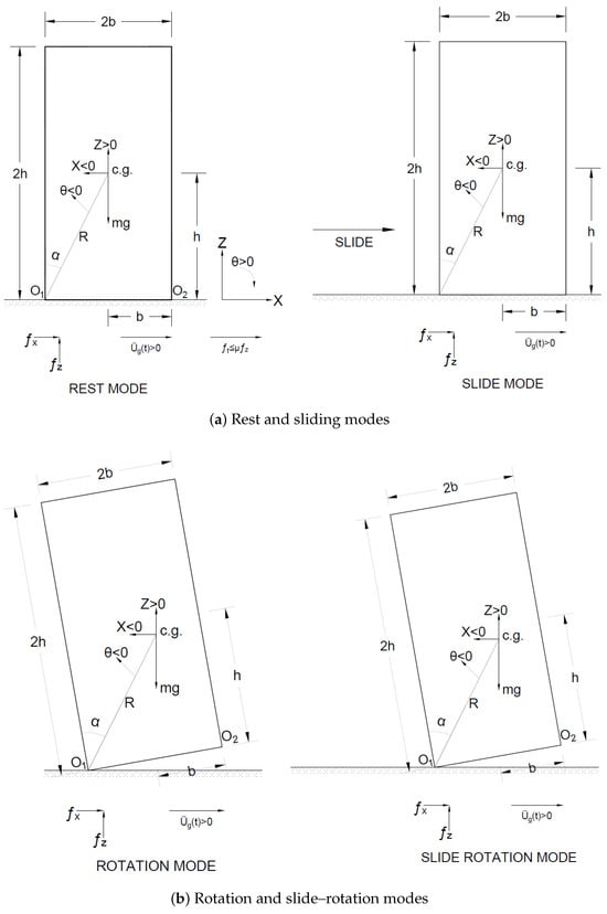
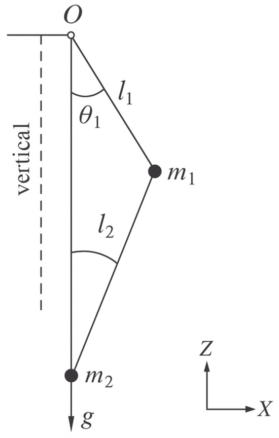
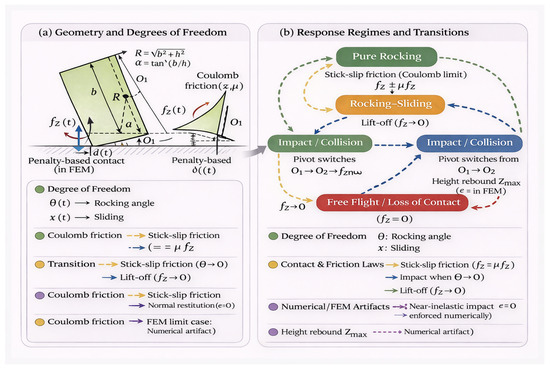
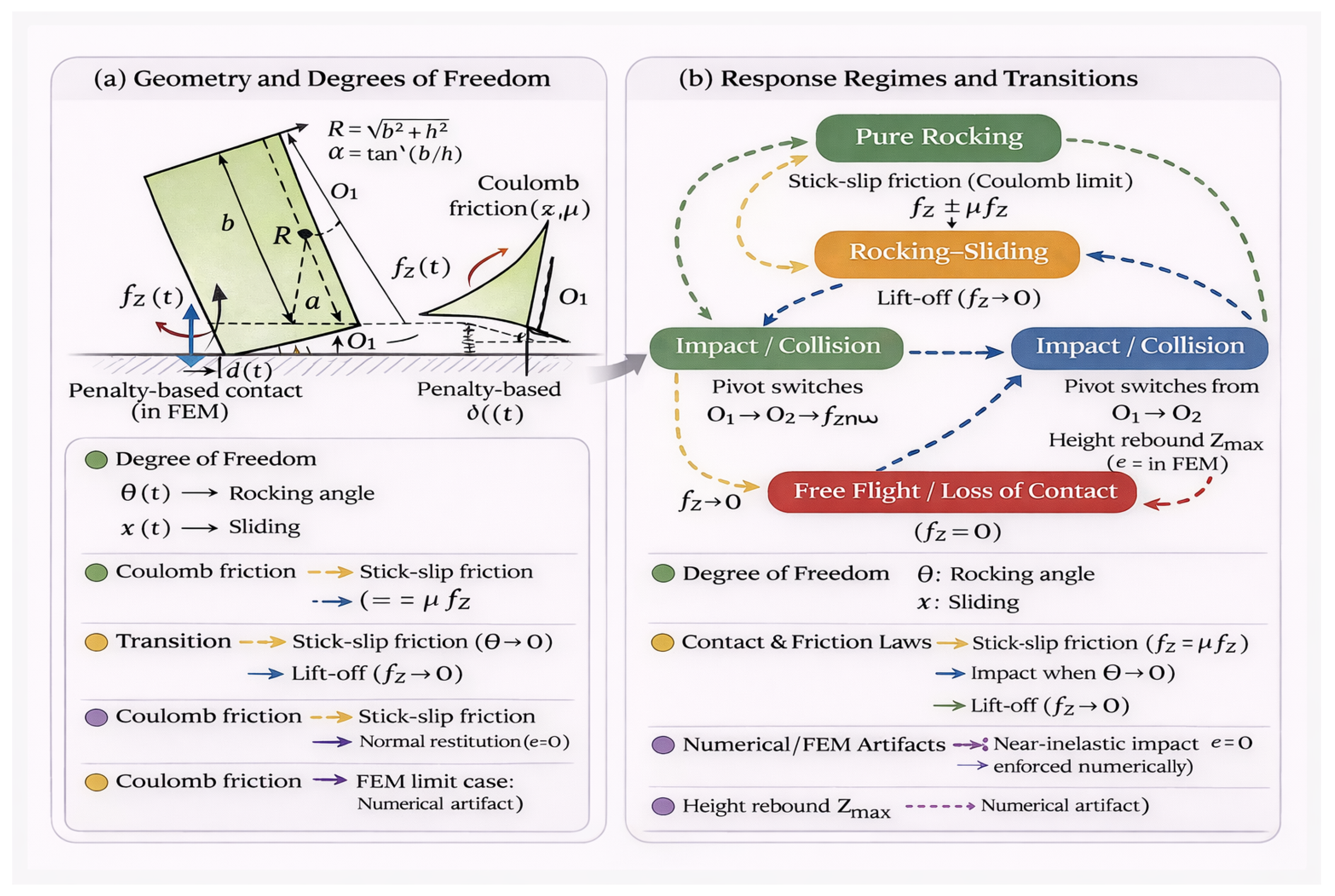
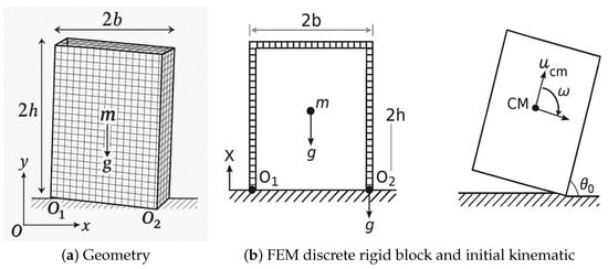
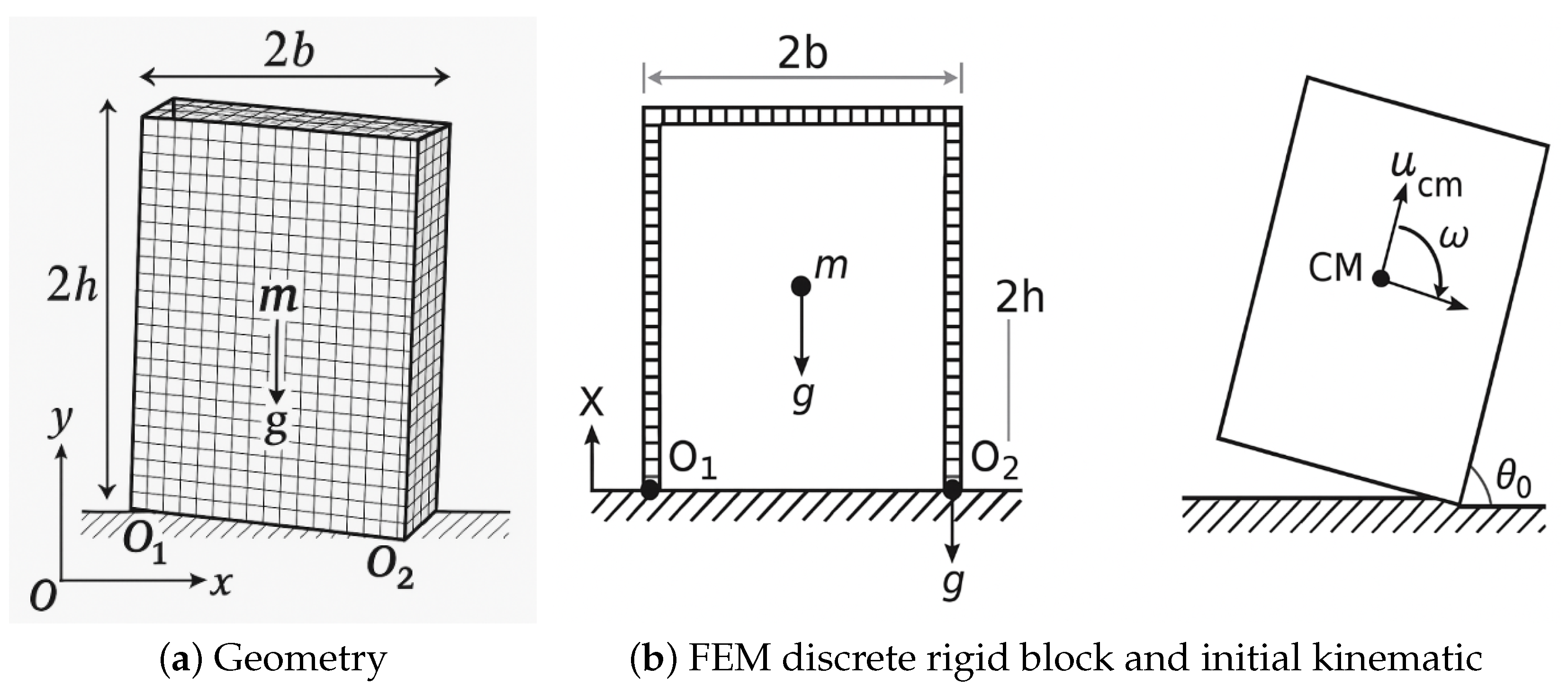
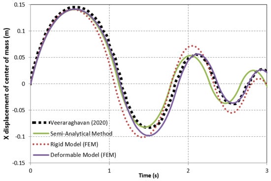
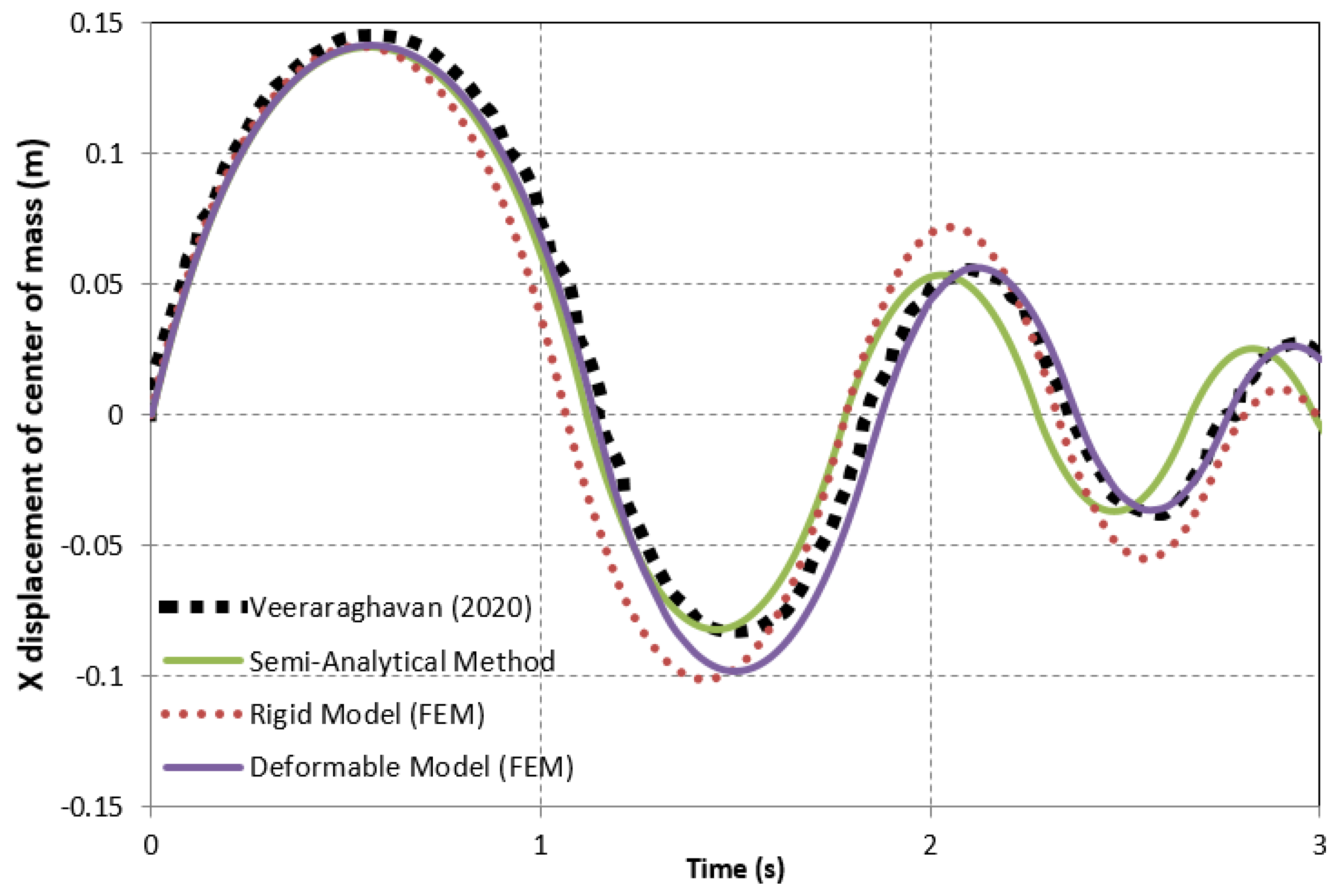
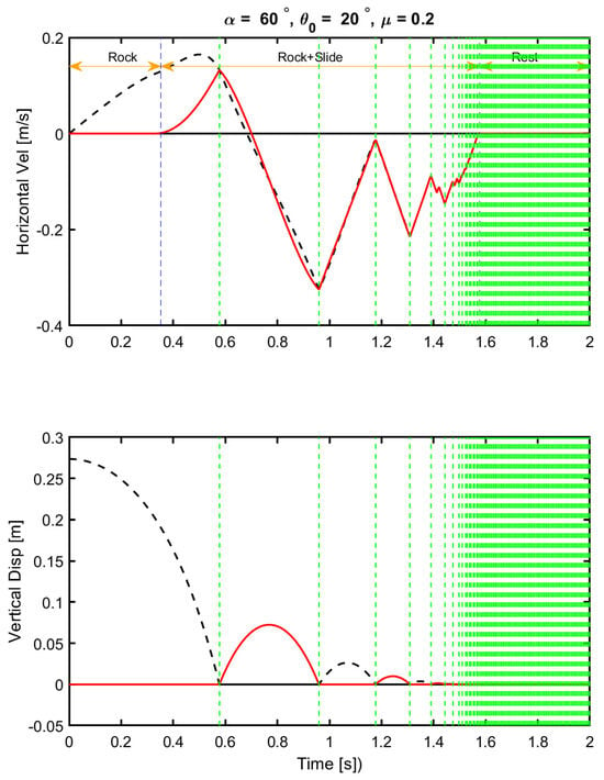
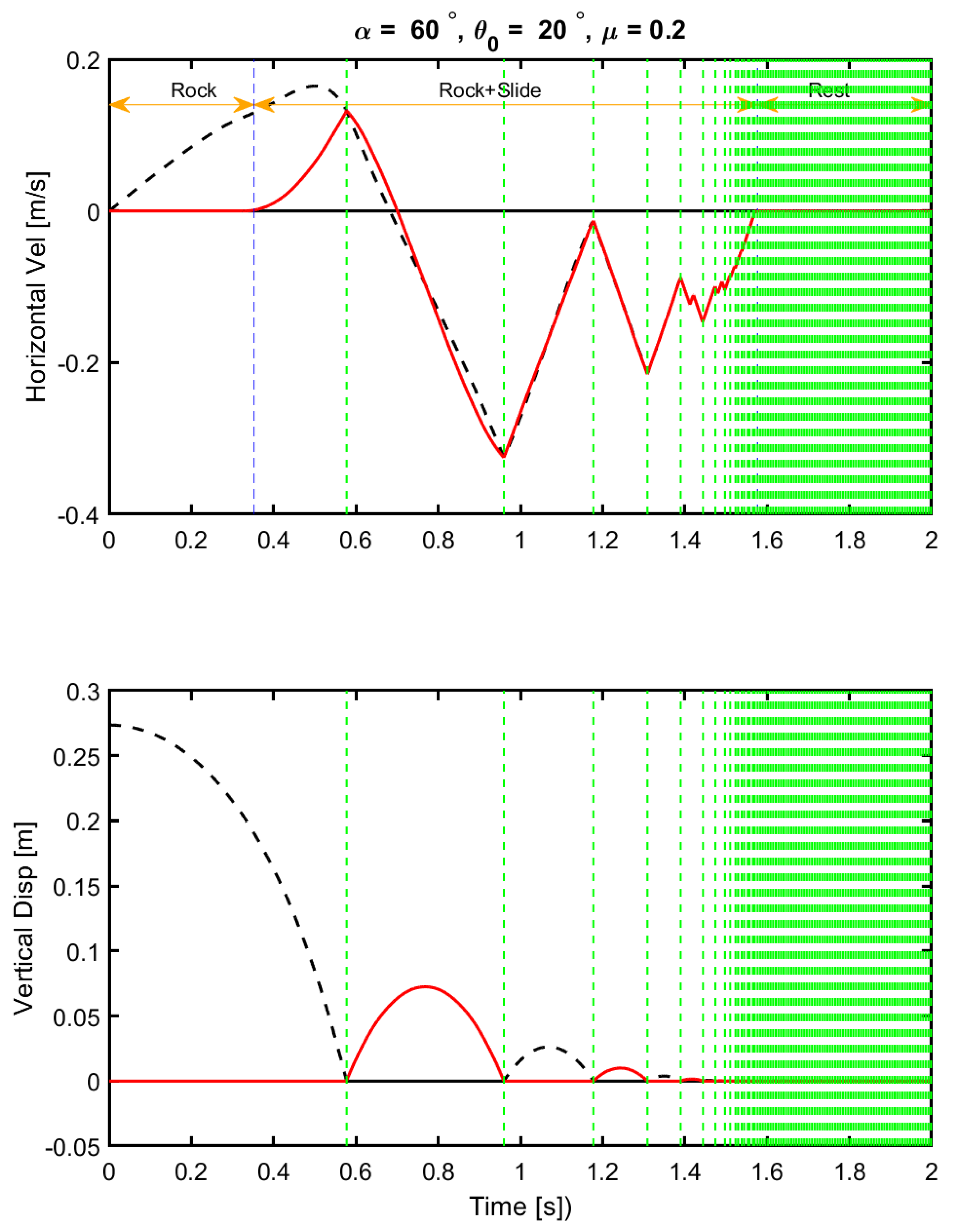
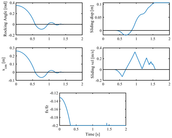
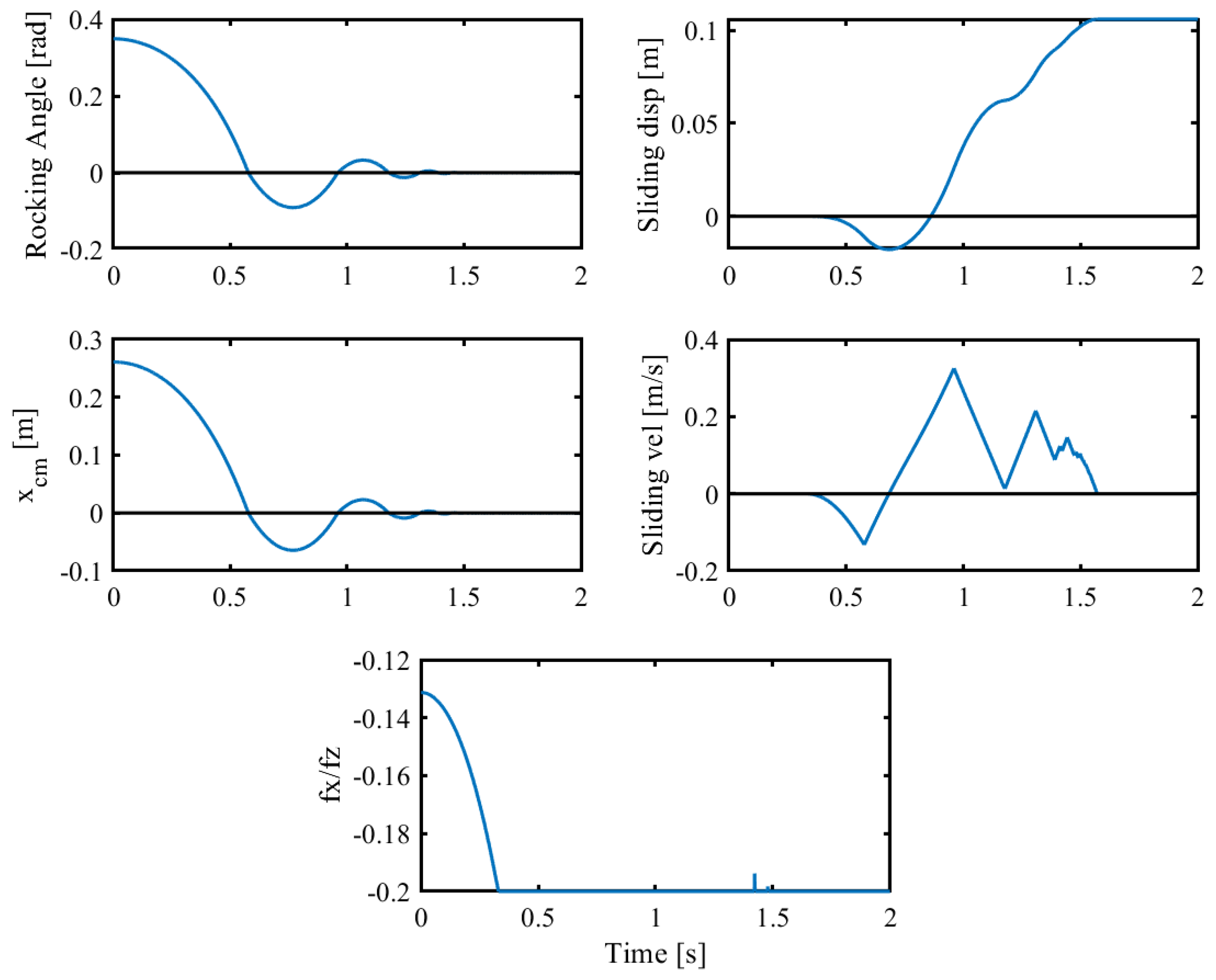
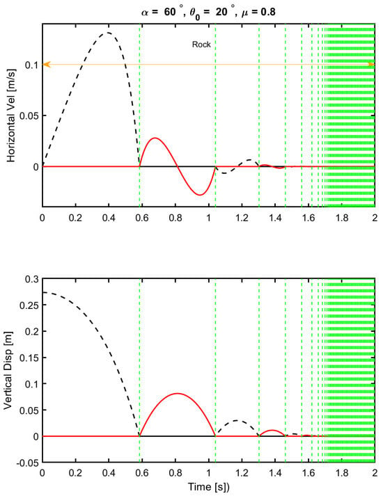
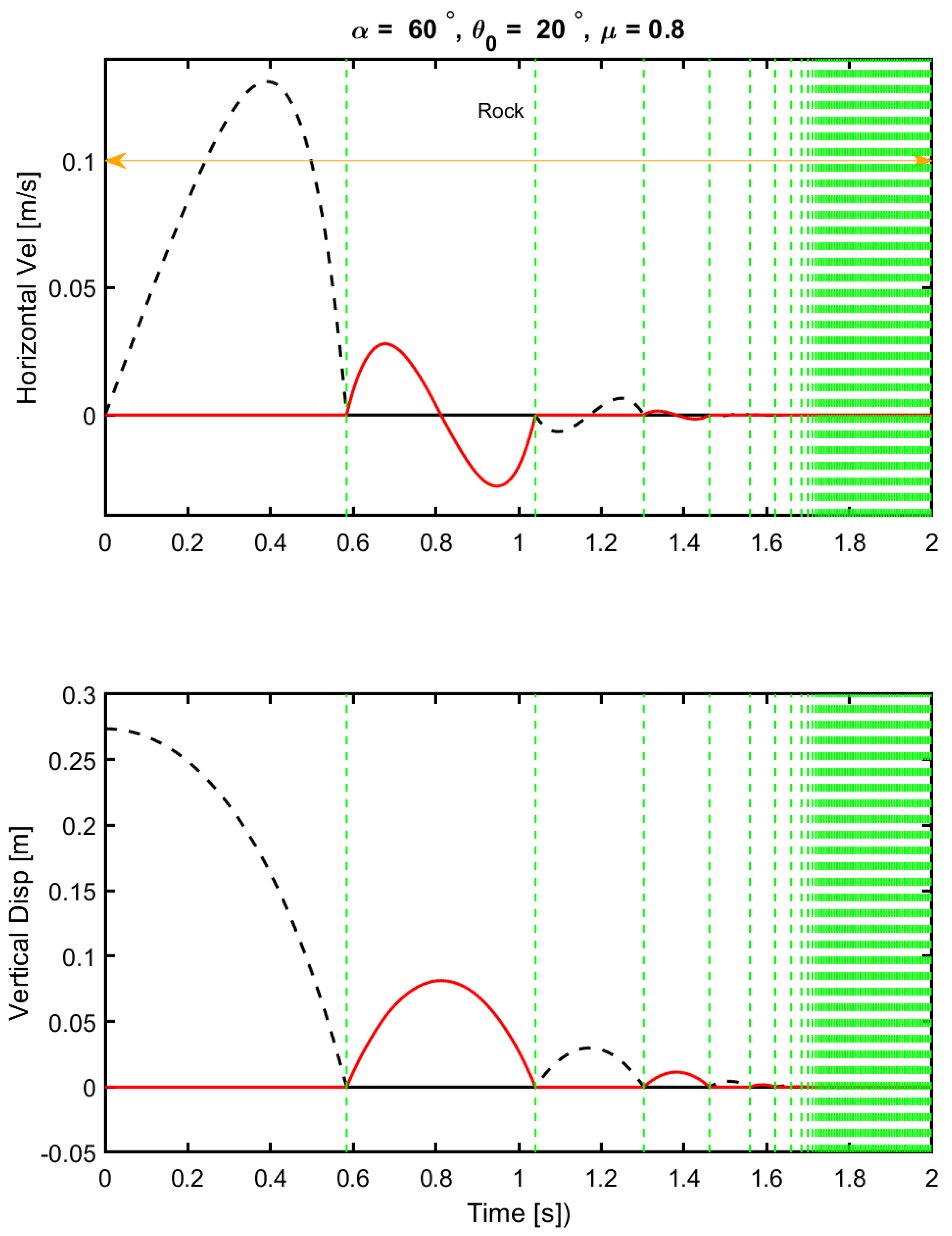
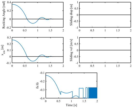
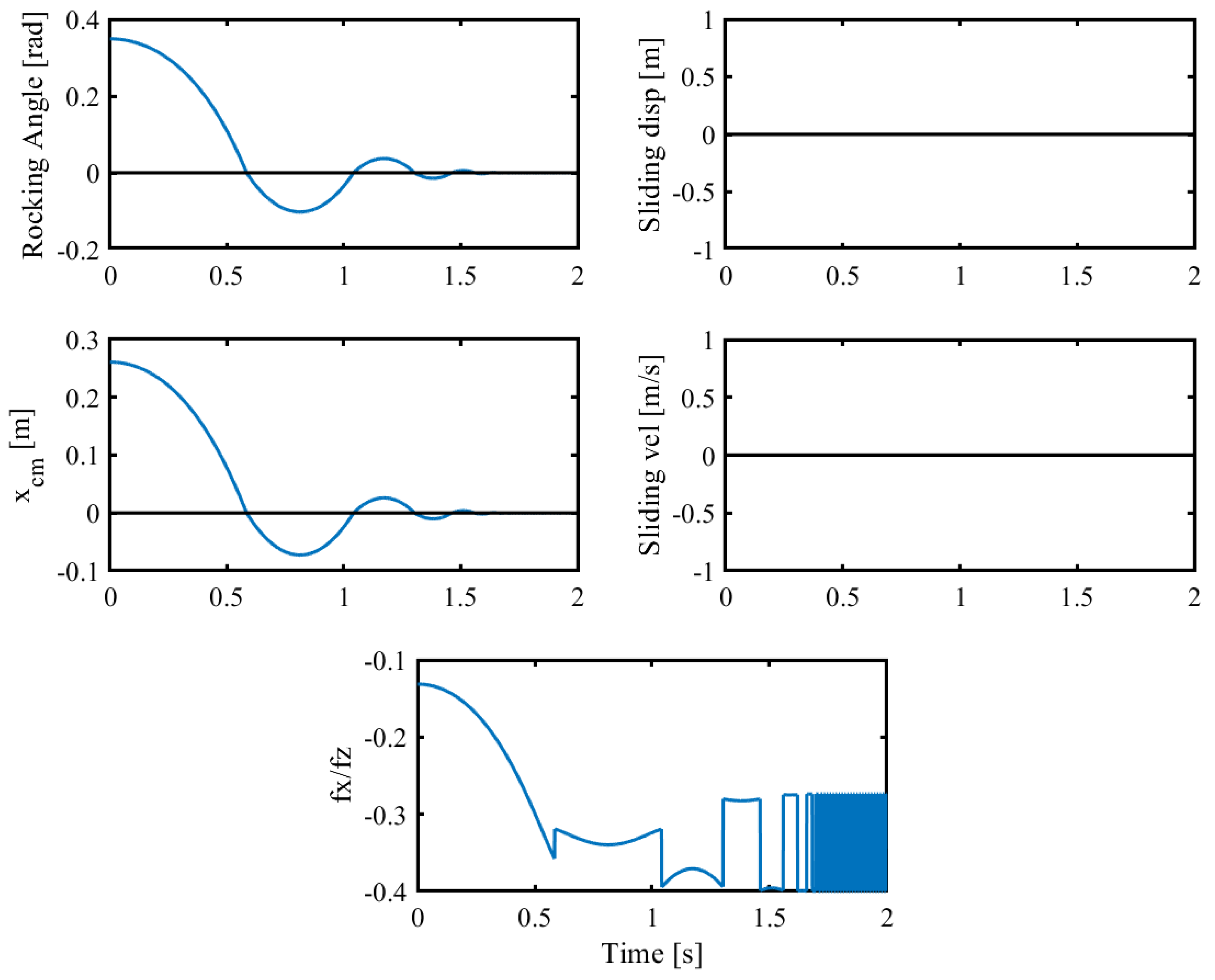
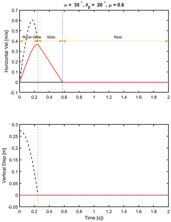
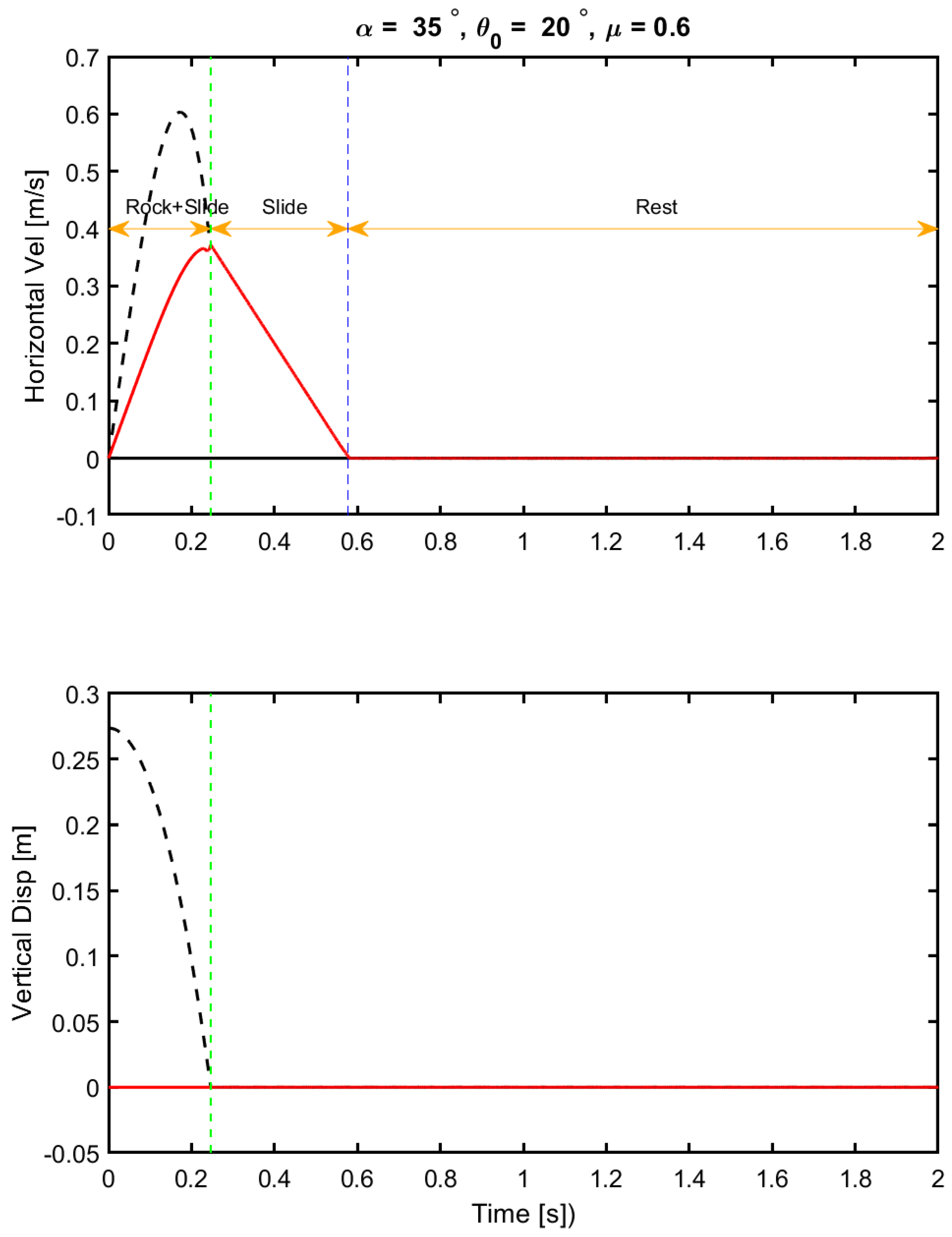
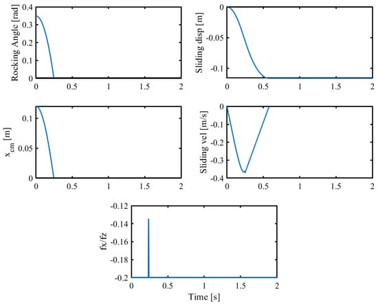
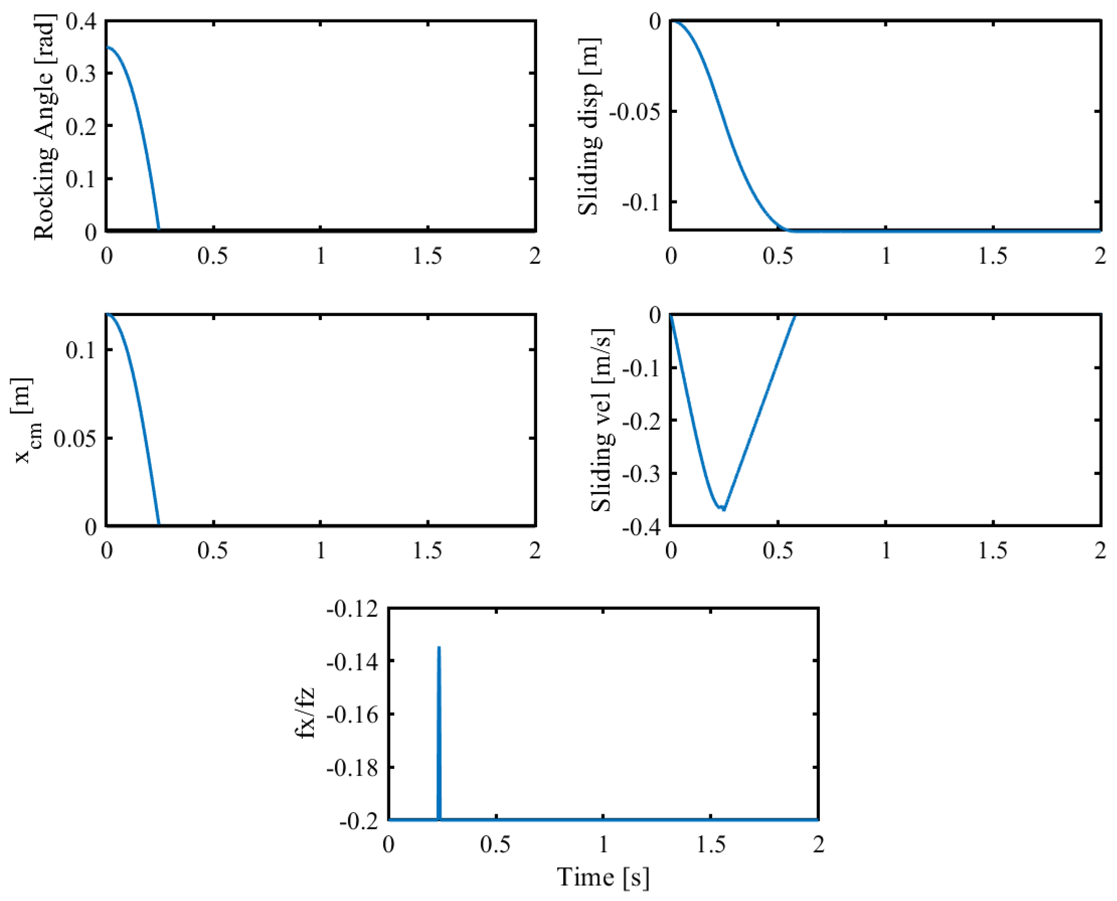
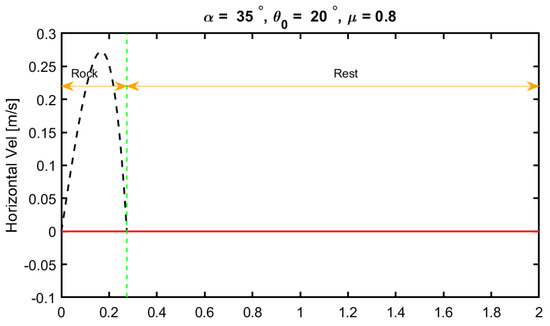
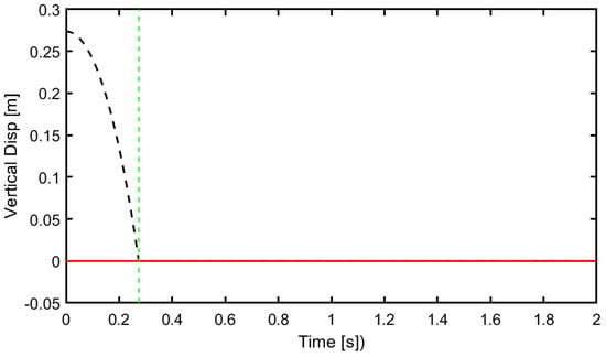
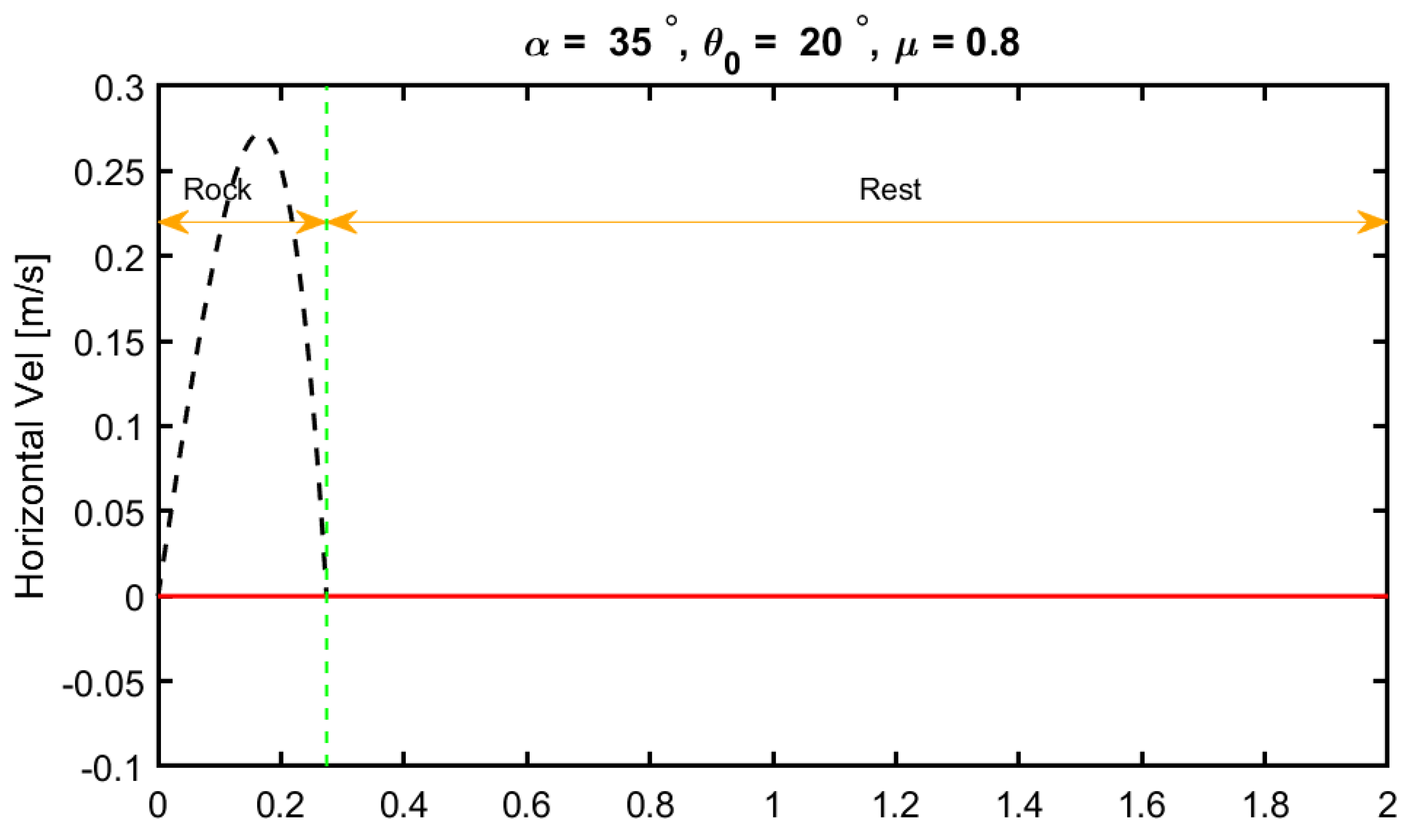
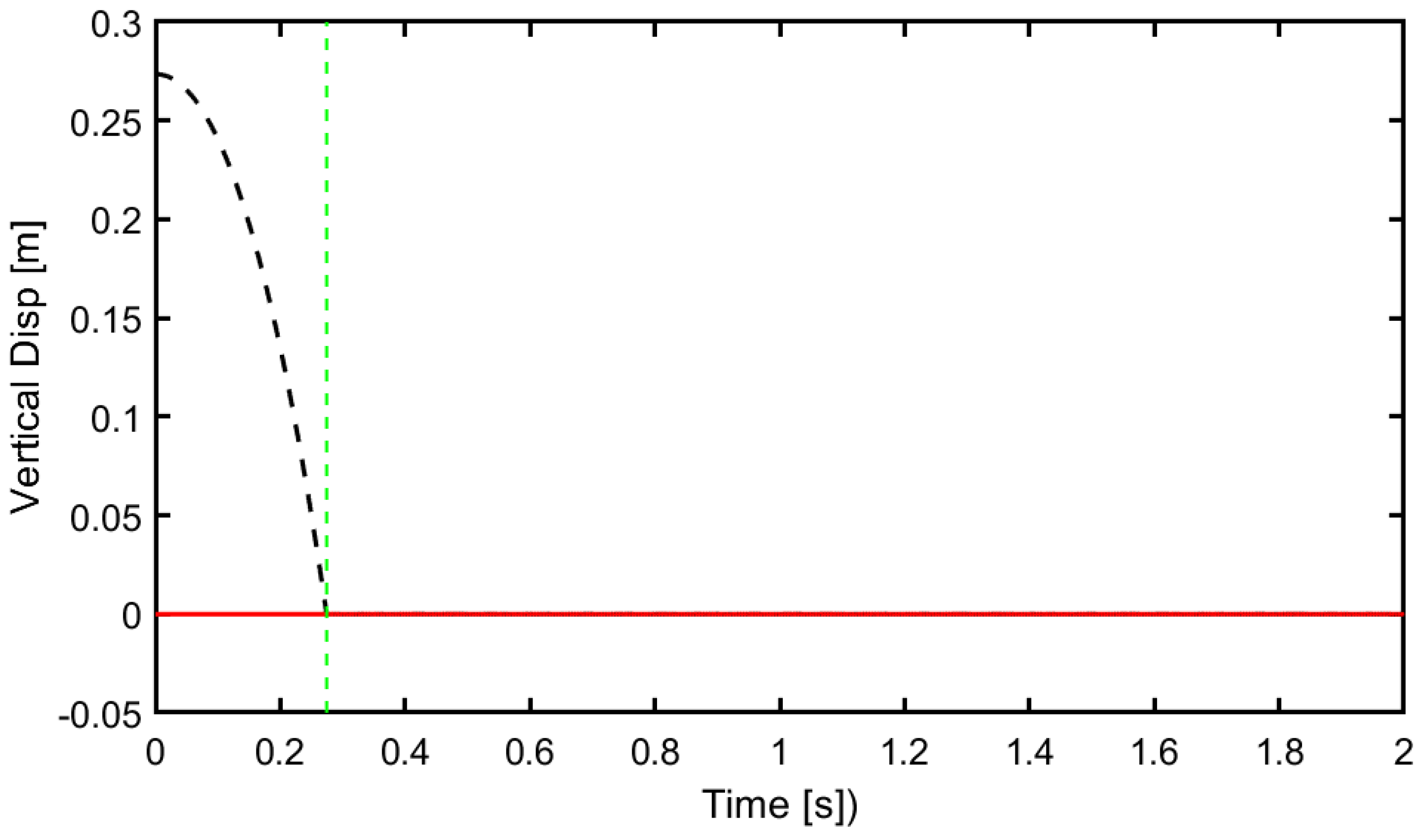
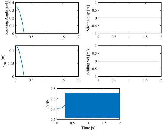
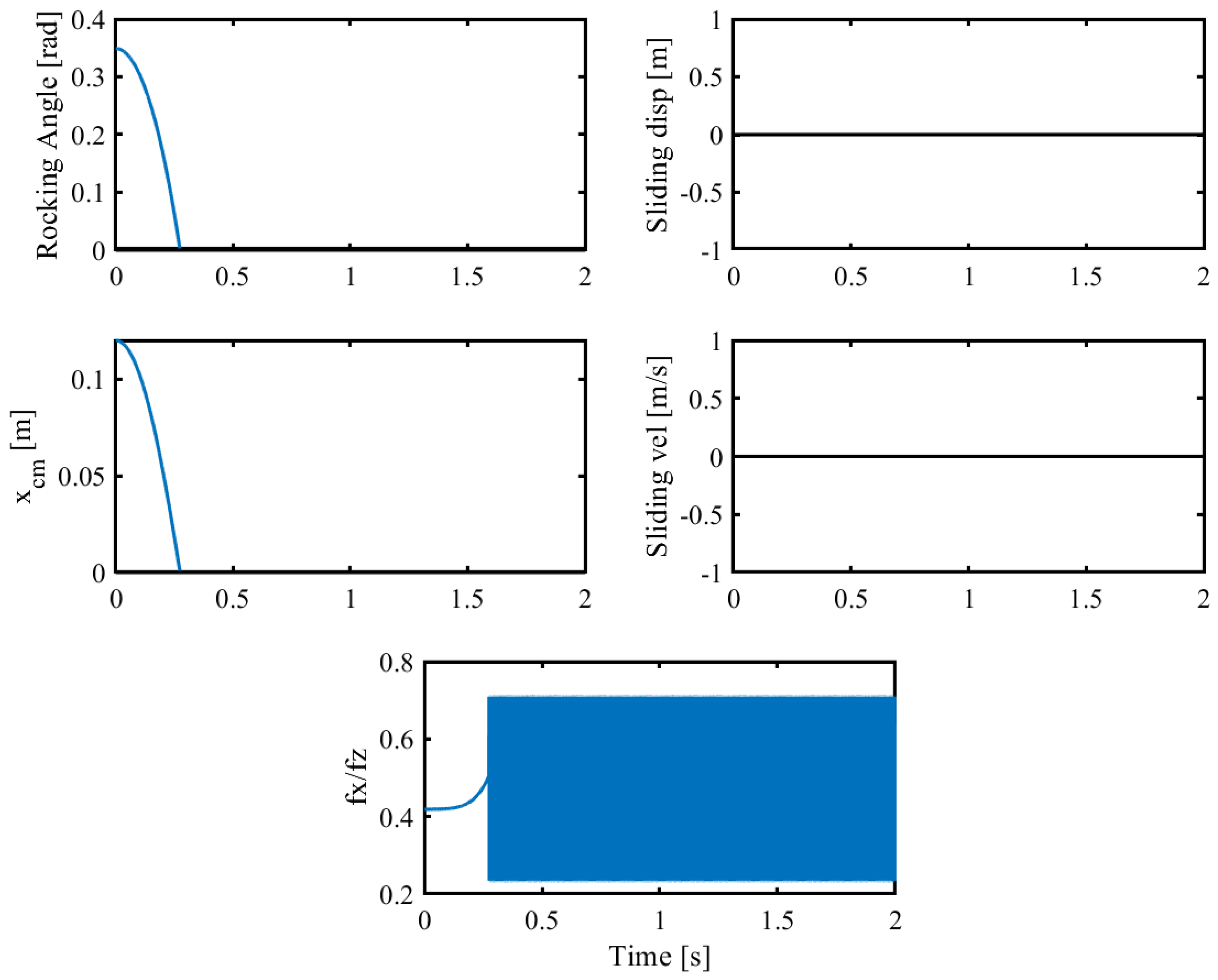
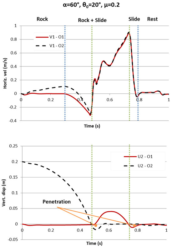
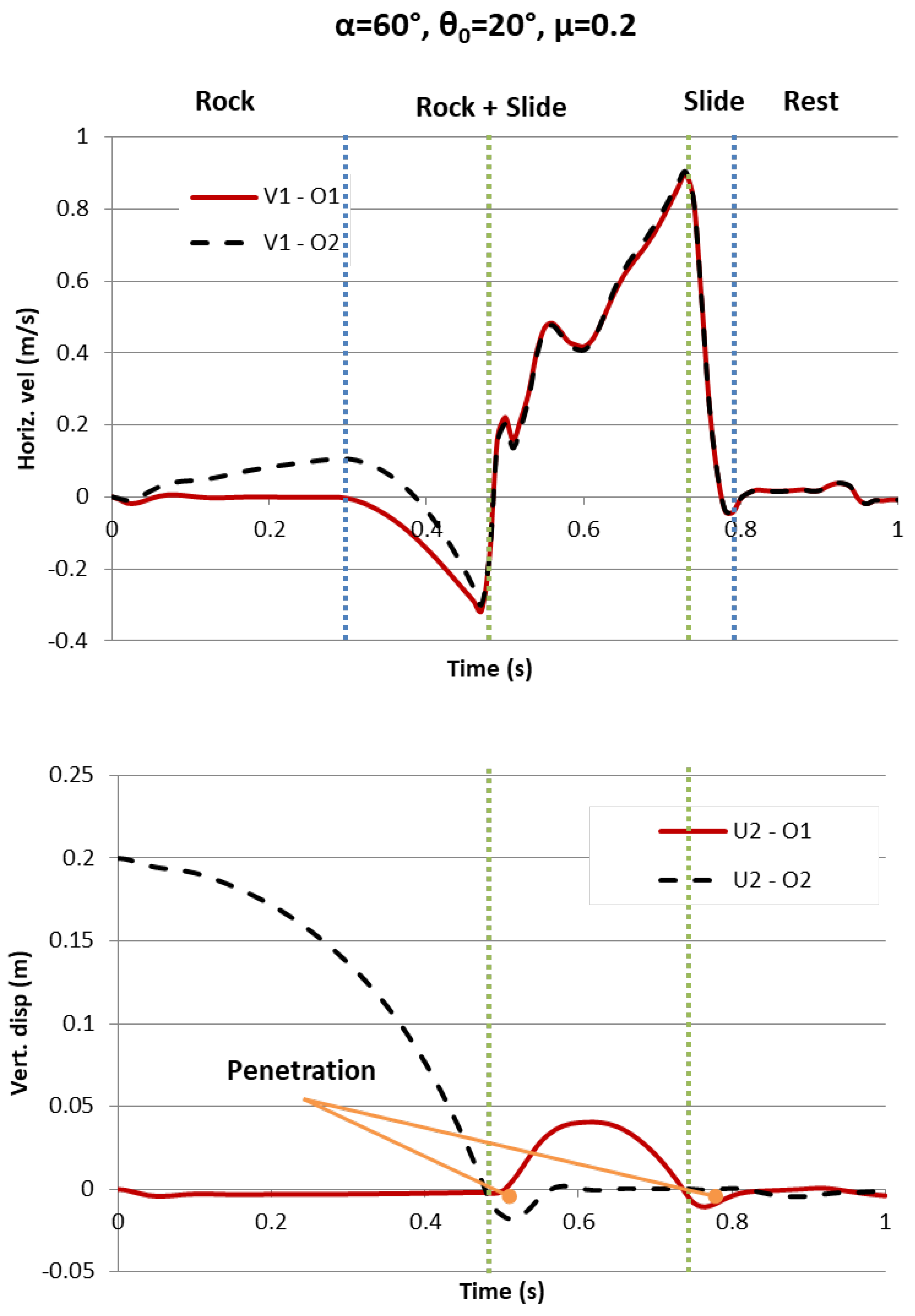
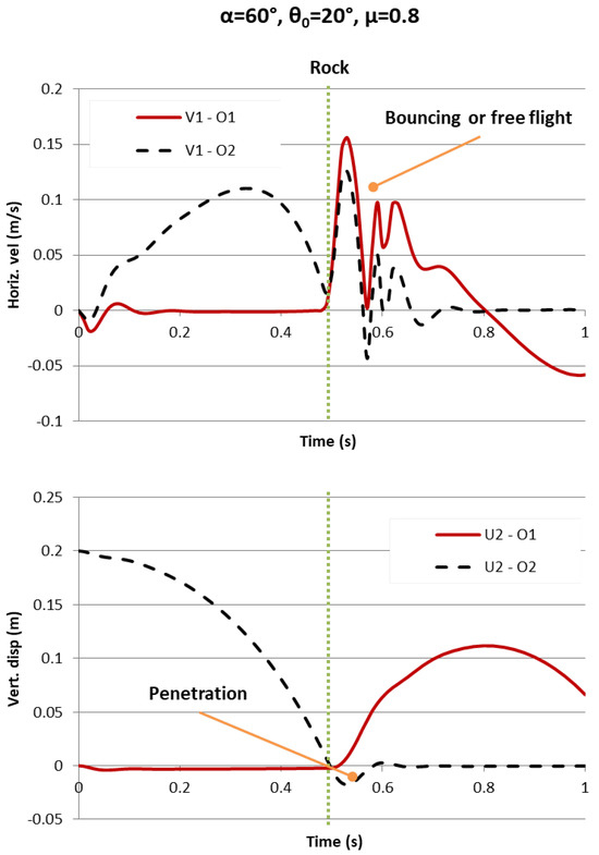
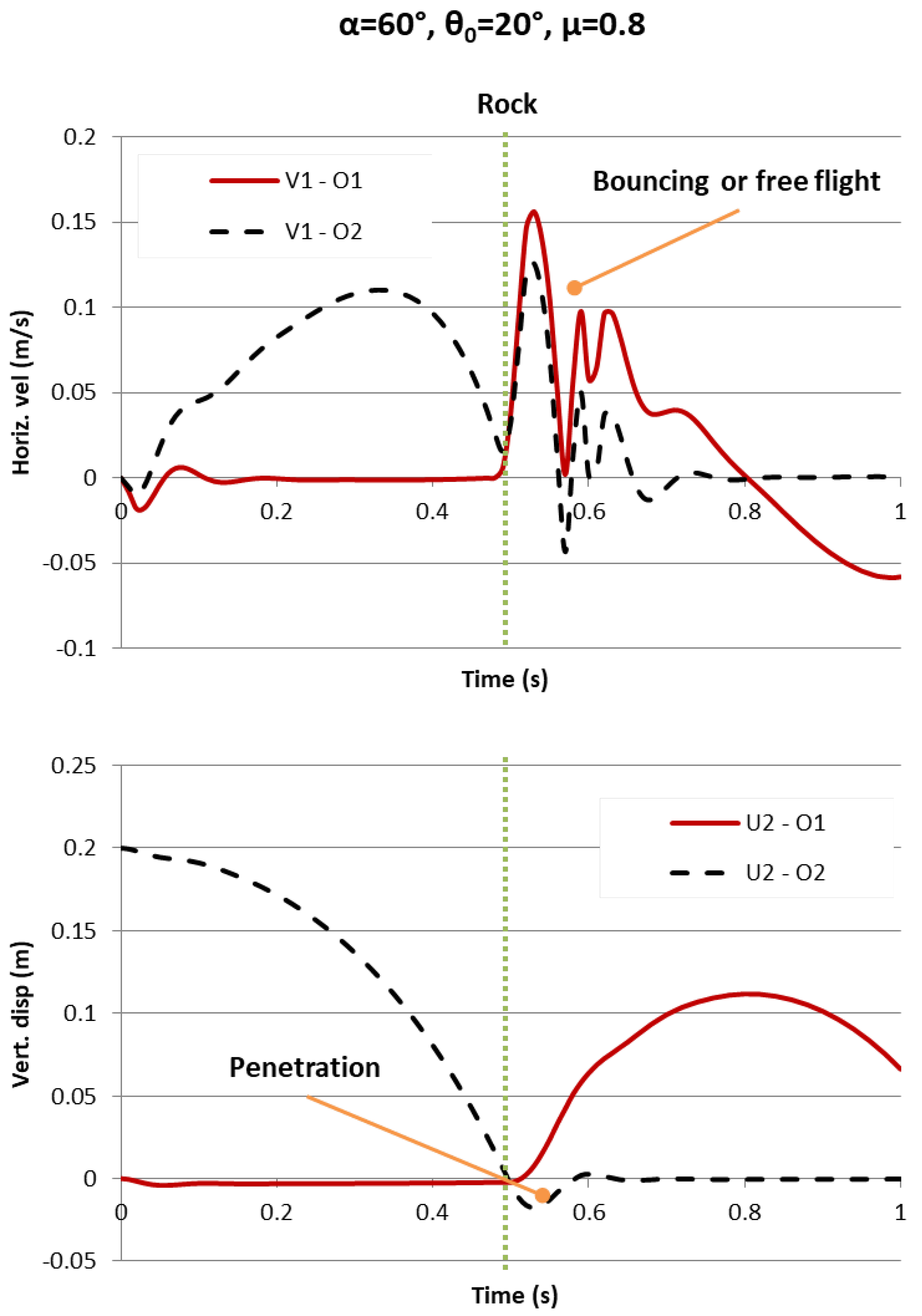
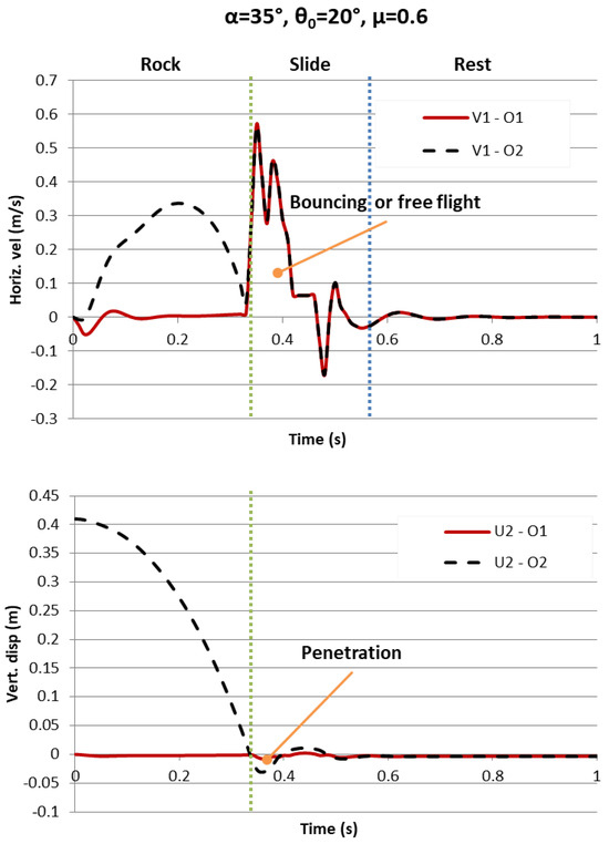
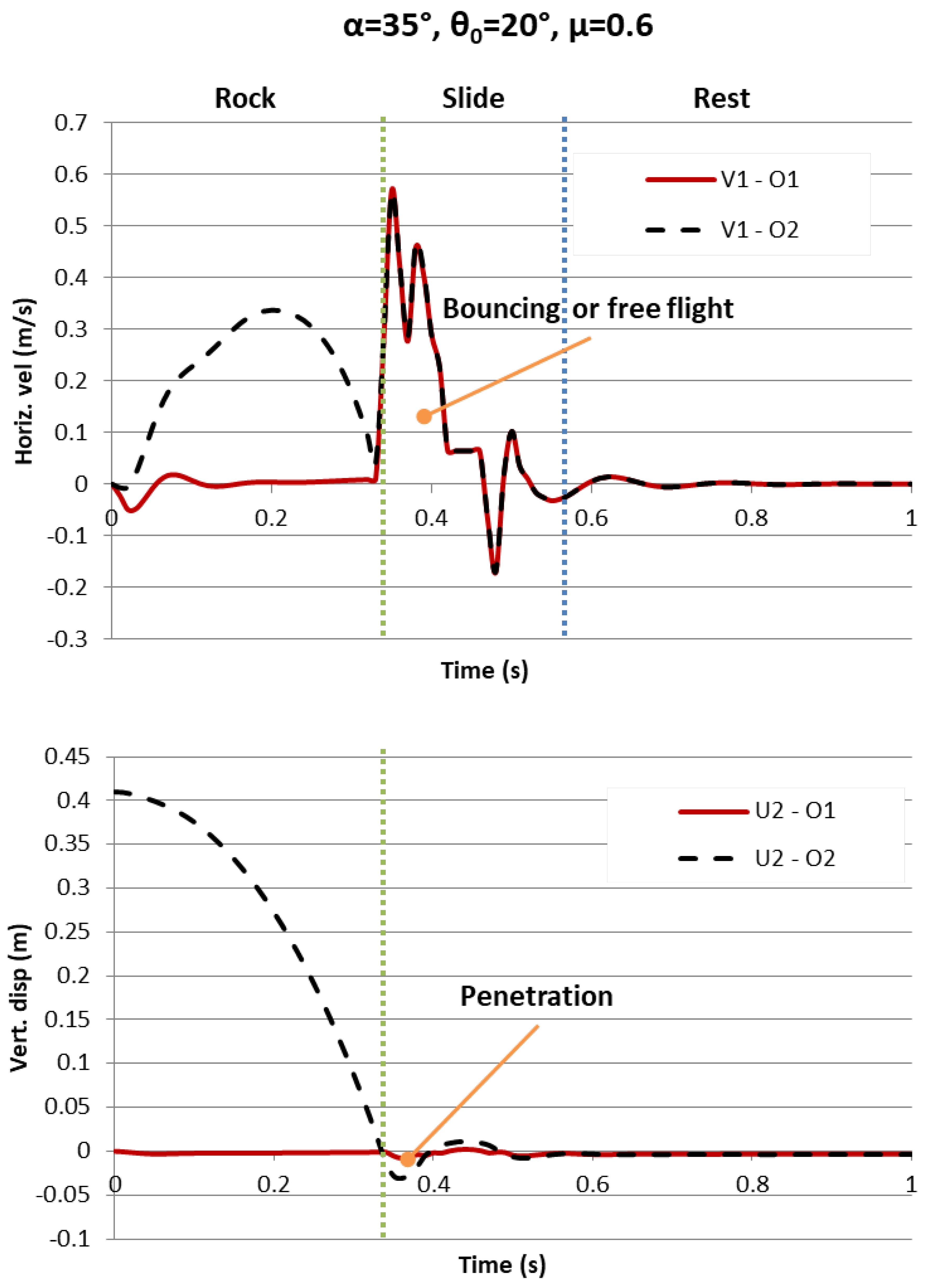
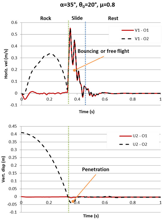
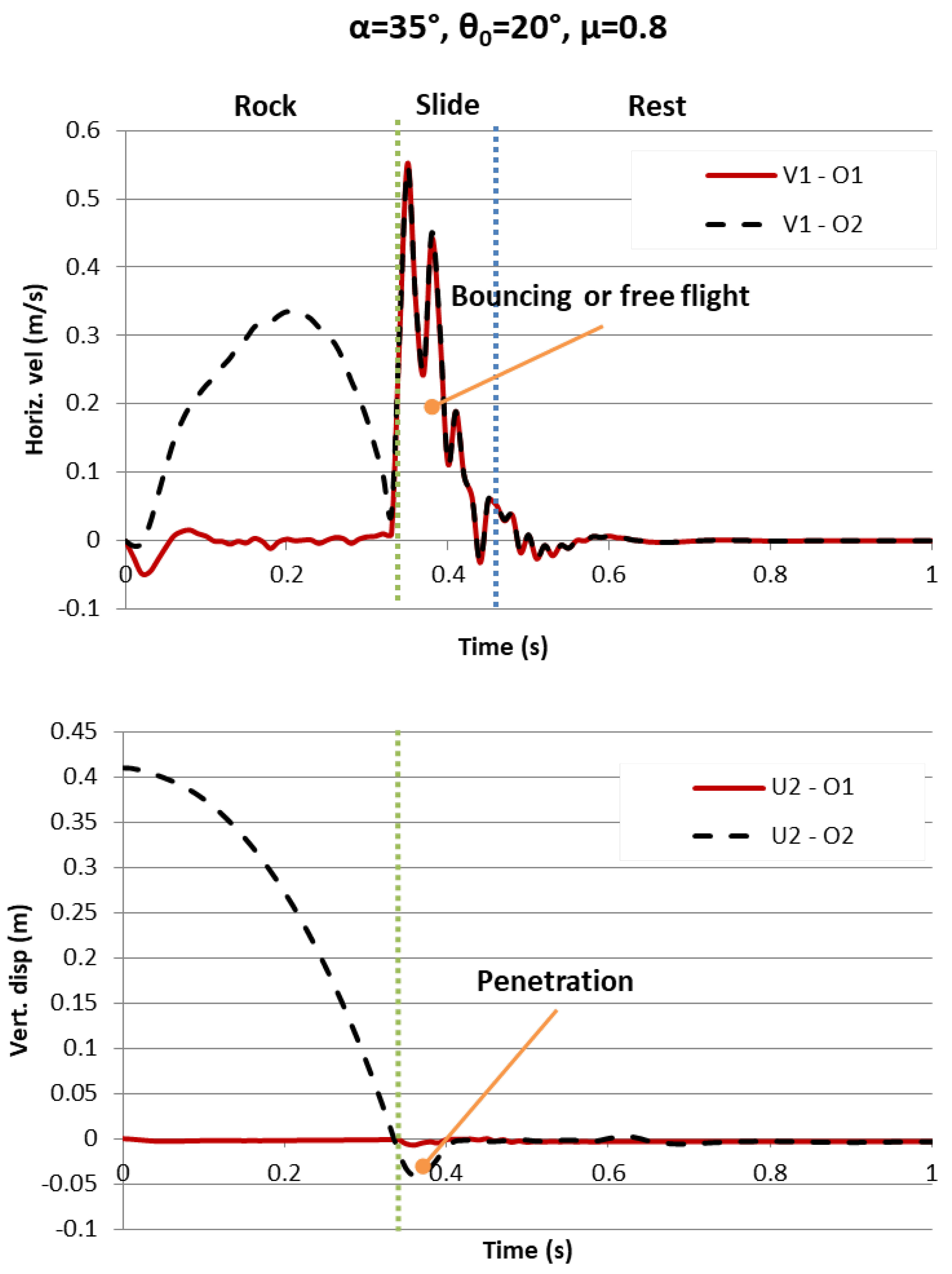
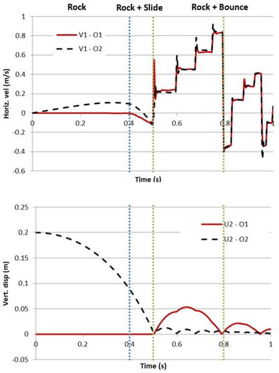
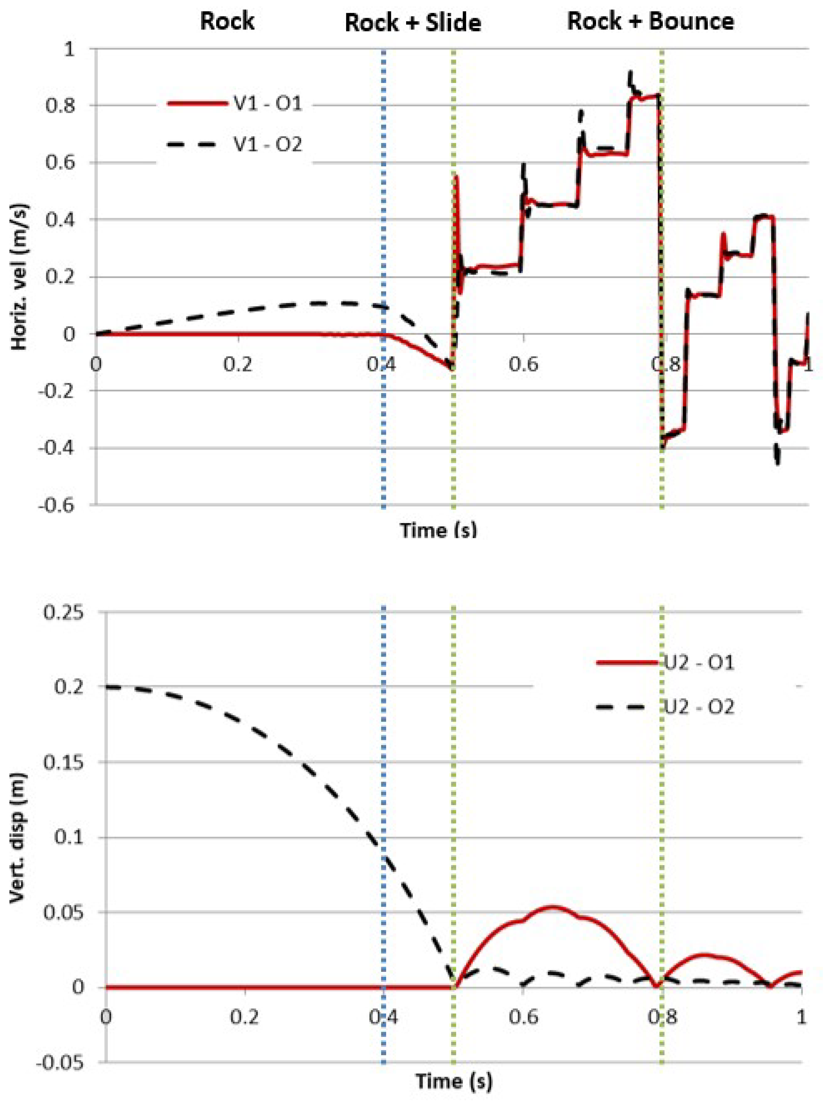
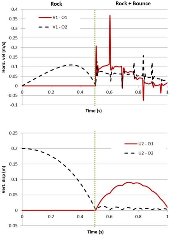
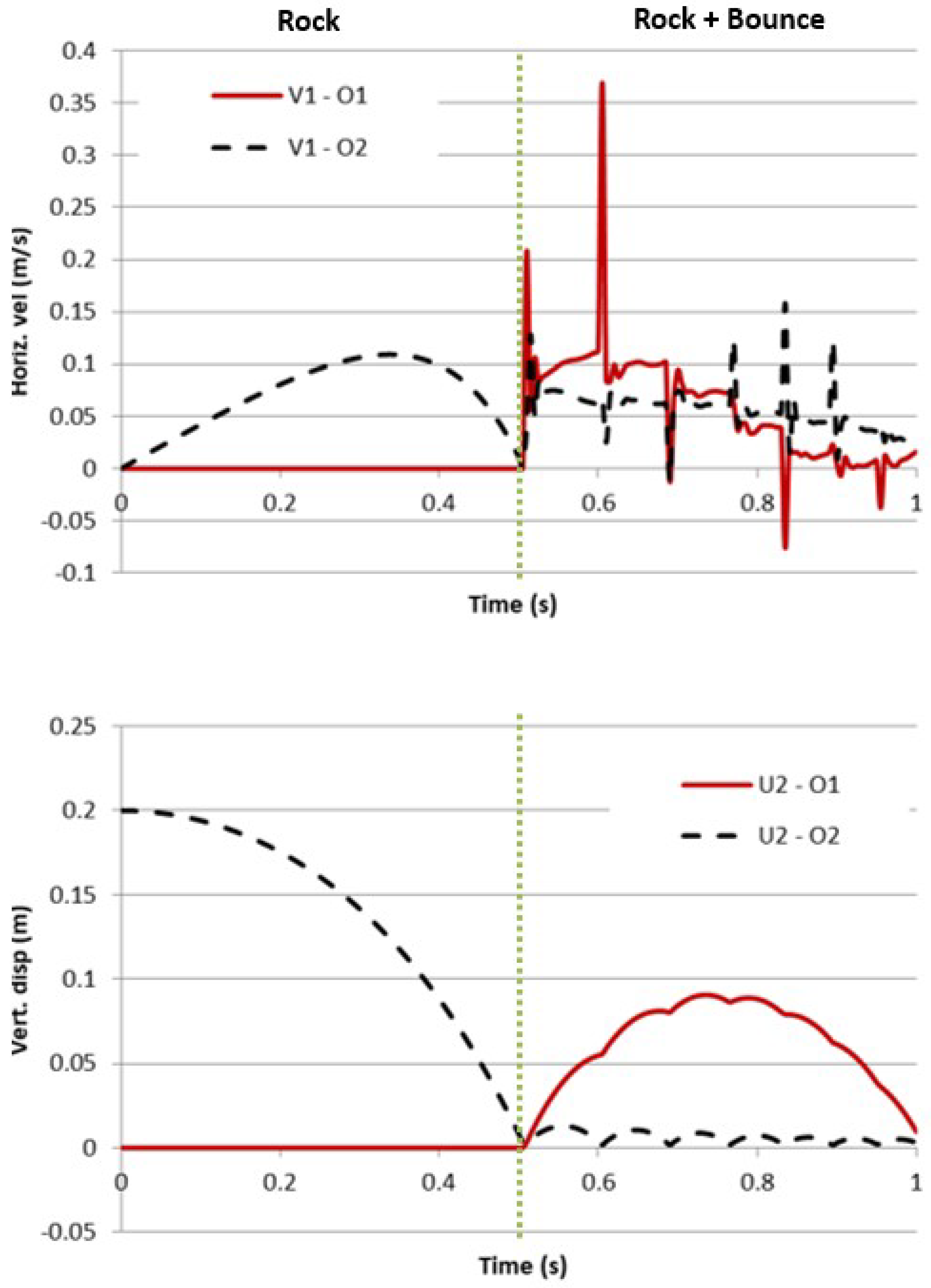
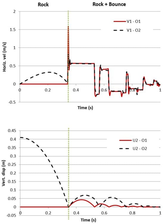
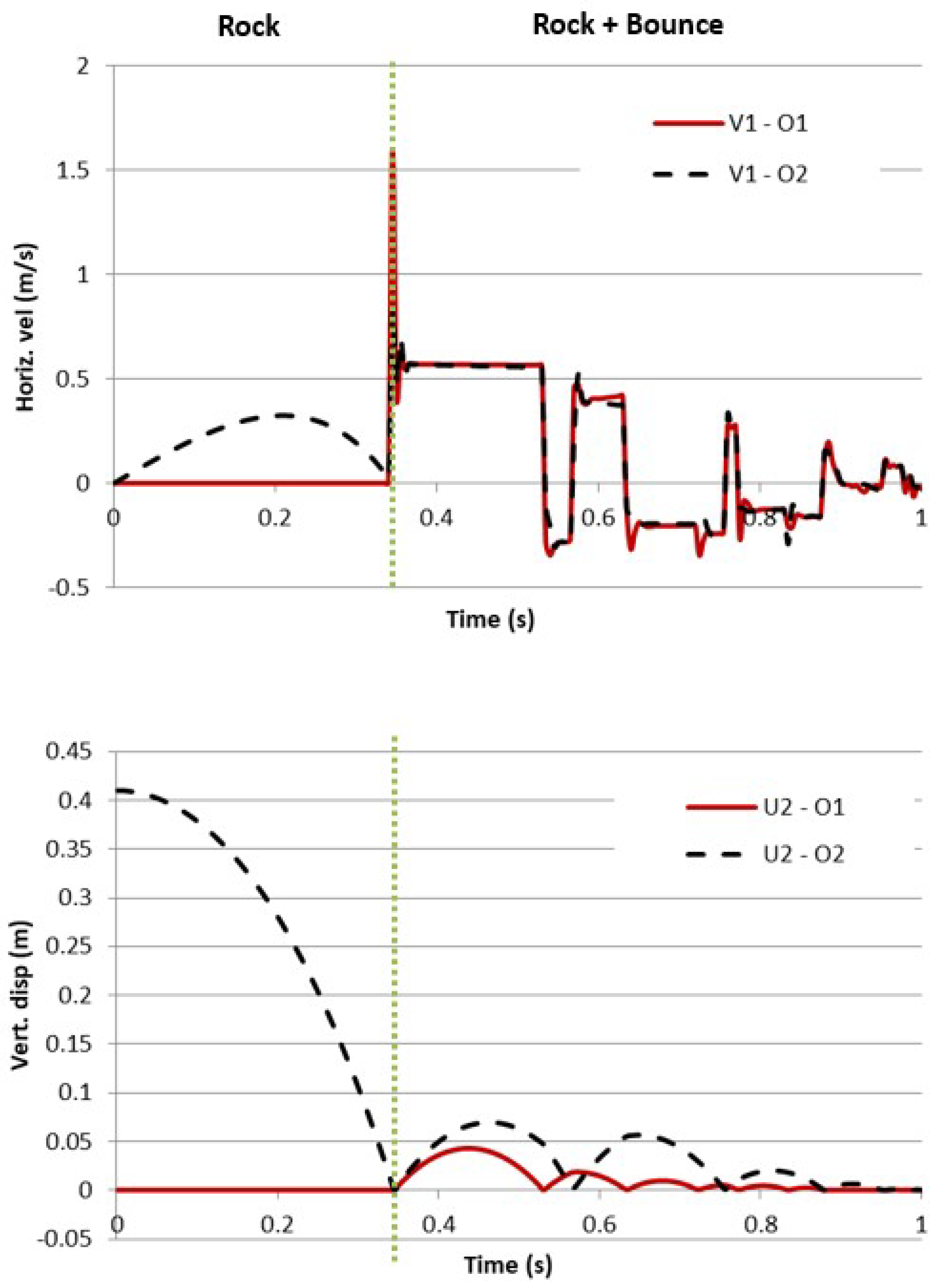
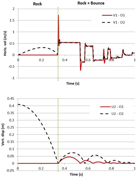
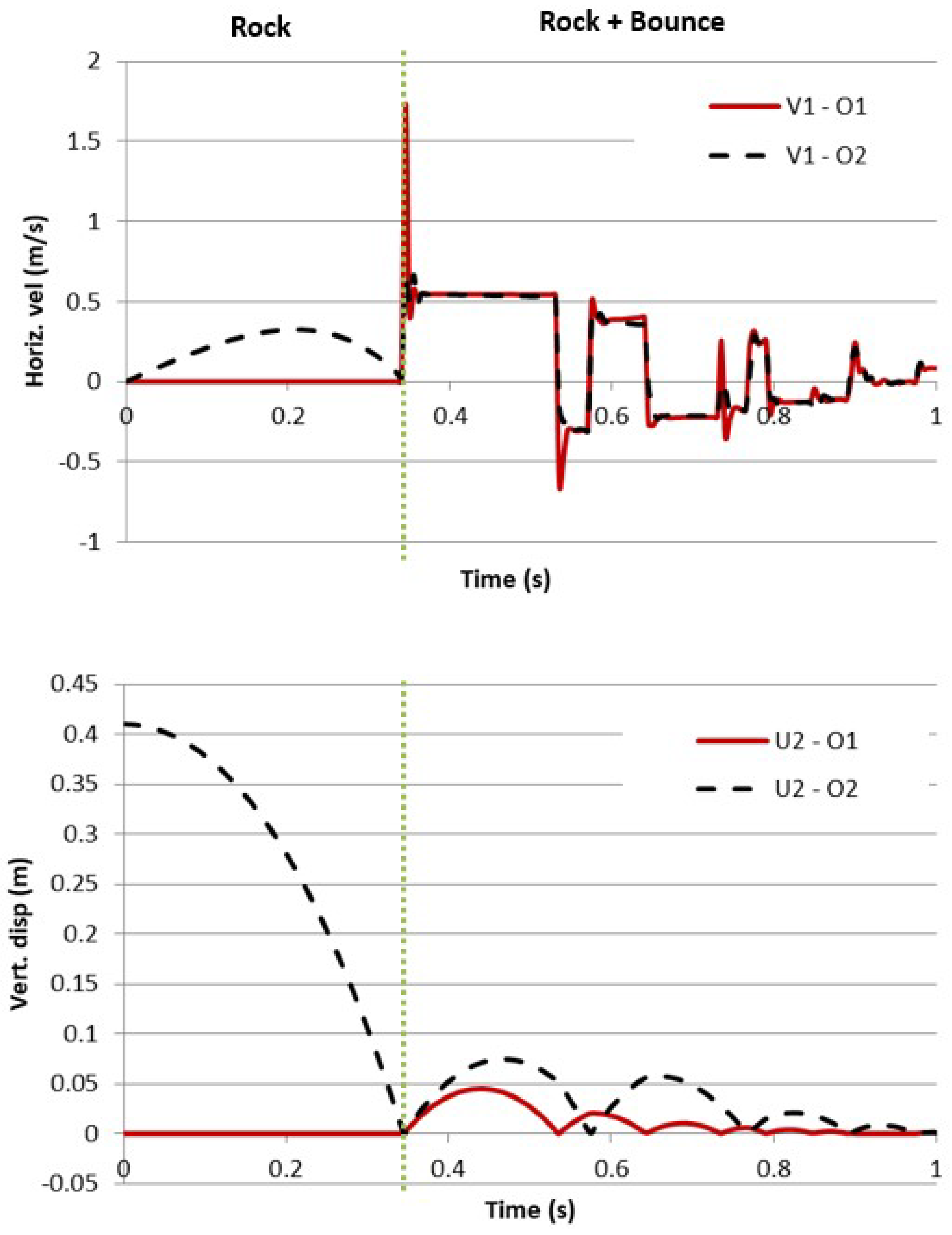
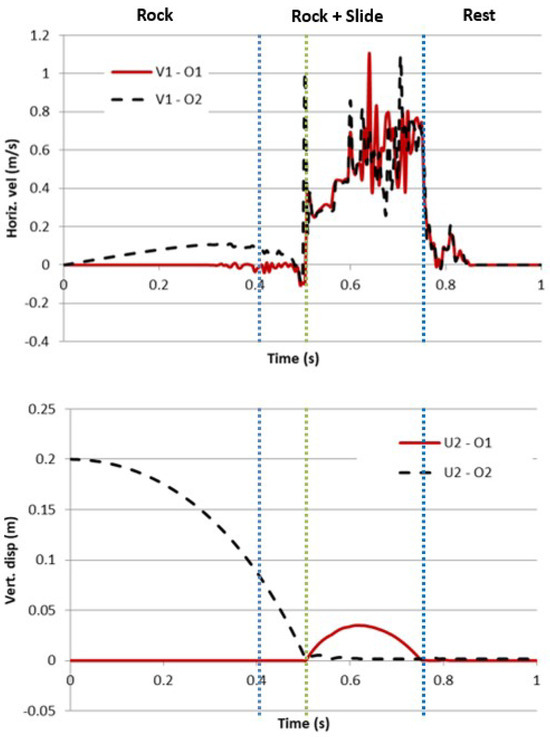
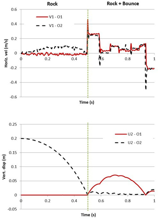
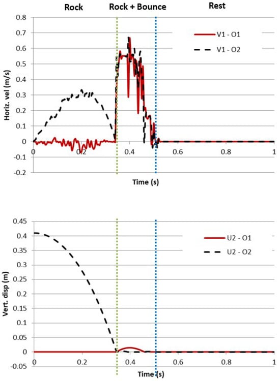
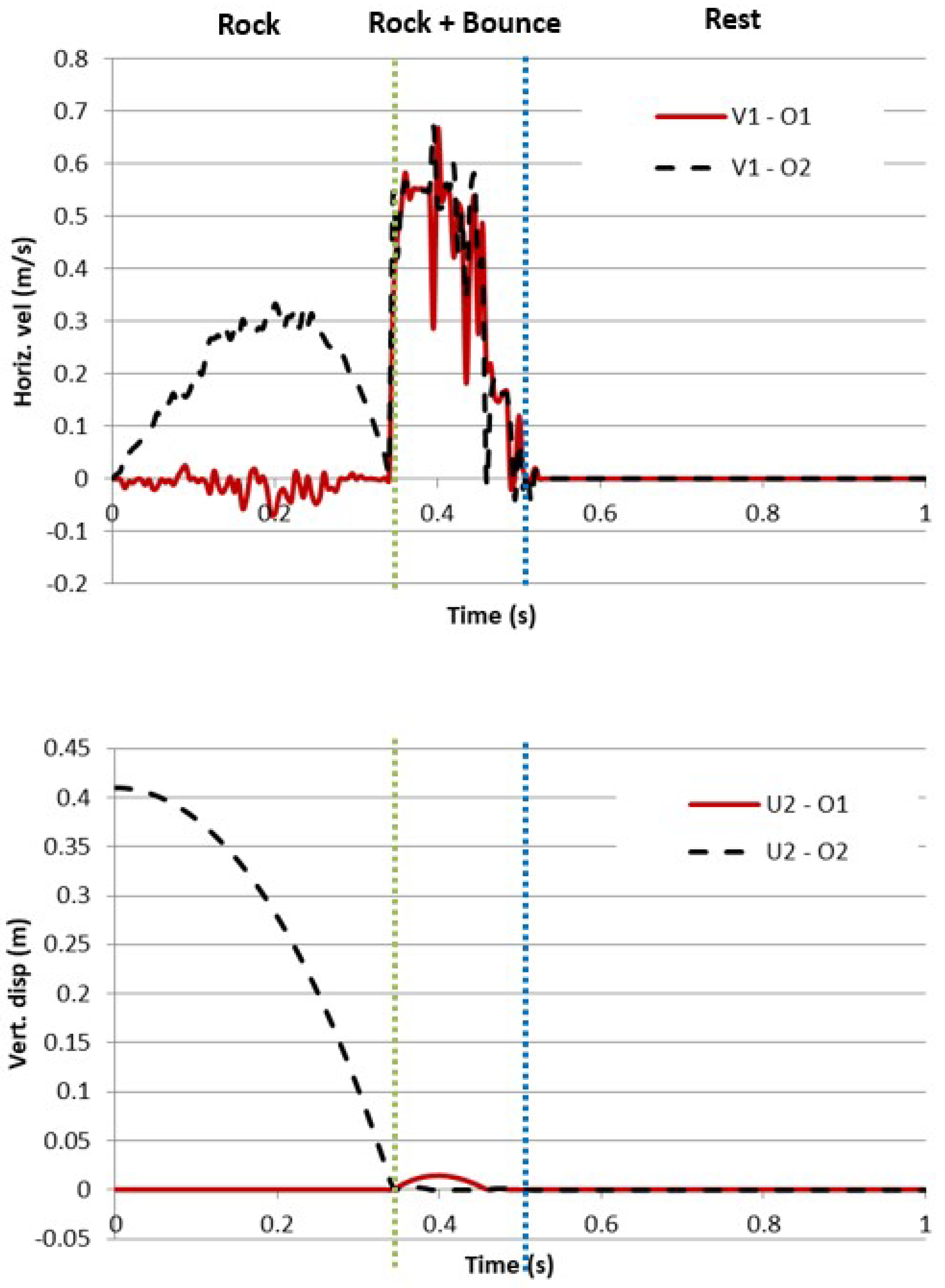
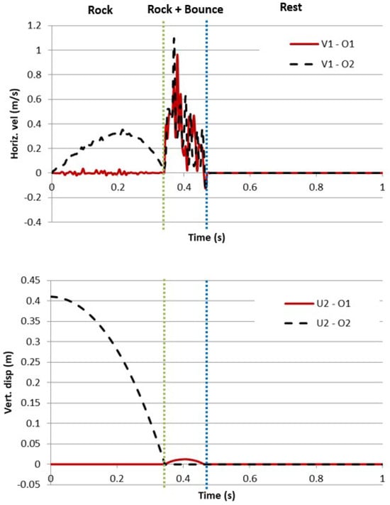
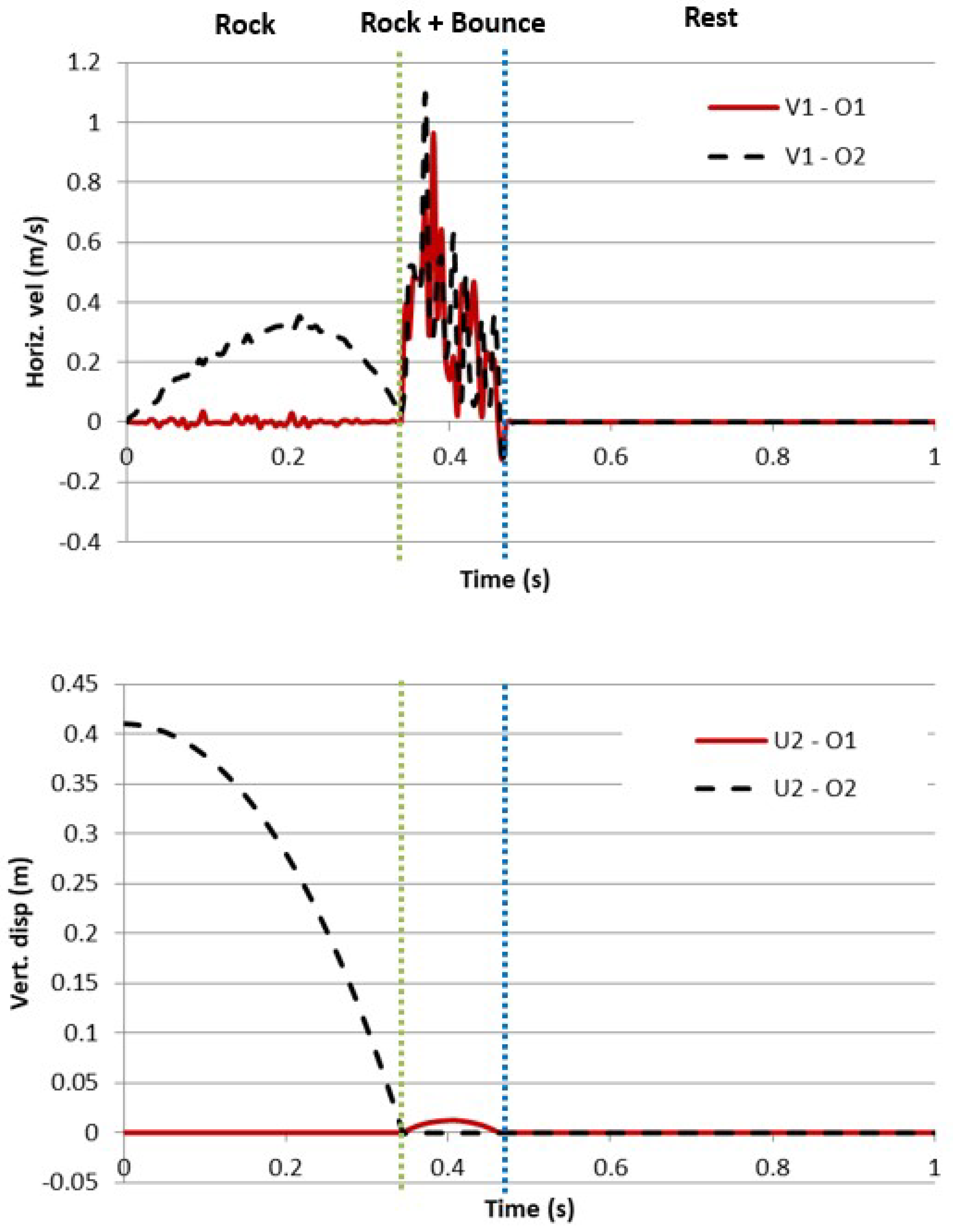

Disclaimer/Publisher’s Note: The statements, opinions and data contained in all publications are solely those of the individual author(s) and contributor(s) and not of MDPI and/or the editor(s). MDPI and/or the editor(s) disclaim responsibility for any injury to people or property resulting from any ideas, methods, instructions or products referred to in the content. |
© 2026 by the author. Licensee MDPI, Basel, Switzerland. This article is an open access article distributed under the terms and conditions of the Creative Commons Attribution (CC BY) license.