


Abstract
Conserving biodiversity requires identifying and prioritizing critical habitats at a fine scale, as coarse-scale approaches often fail to address the needs of specialized and threatened species. This study applies a fine-scale prioritization approach across temperate and tropical regions of North America and the Caribbean using a detailed map of 636 ecosystem types and high-resolution Area of Habitat (AOH) data. We then evaluated the current protection status and risk of future land use changes for each habitat type and prioritized them for conservation. Our results revealed that 38% of the area was identified in the top quartile of high-priority habitats, with 56 (33%) of identified IUCN threatened ecosystem types captured within these areas. Top priority habitats include the Meso-American Premontane Semi-deciduous Forest, Central American Caribbean Evergreen Lowland Forest, and Guerreran Dry Deciduous Forest, all characterized by low protection, high projected land-use conversion, and large numbers of threatened and habitat-specialist species, highlighting their urgent conservation importance in Meso-American and Caribbean tropical forests. Our findings emphasize the need for targeted conservation strategies that consider finer-scale habitat classifications and species requirements to improve the precision of conservation planning, especially where already at-risk species and ecosystems are located, and human land use intensities are high.
1. Introduction
1.1. Biodiversity Conservation in North America and the Caribbean
Temperate and Tropical North America, including the Caribbean, supports tremendous biodiversity at genetic, species, and ecosystem levels [1]. This region spans sub-boreal to tropical latitudes and includes a wide variety of terrestrial ecosystem types, from forests and grasslands to deserts, freshwater wetlands, and coastal mangroves. It encompasses about 8.5% of the global land area (excluding Antarctica). The natural ecosystem types found here provide habitat essential to both common and rare flora and fauna that, over time, have defined the ecological processes and selective pressures on these species [2]. Several regions across North America, such as the Caribbean, Mesoamerica, and the southeastern US, are among the world’s richest biodiversity hotspots, harboring some of the highest numbers of animal and plant species, and endemics found nowhere else on Earth [3,4].
However, despite advancements in protected area systems, threatened biodiversity is still inadequately protected [5,6,7]. For example, within the United States, only 12% of land currently falls under relatively strict formal protection. This leaves about 40% of animals, 34% of plants, and 40% of terrestrial ecosystem types at risk for extinction or range-wide collapse [8,9,10,11]. About 20% of the land base of the insular Caribbean is designated as a protected area [12]. In this region, islands vary in the degree of protection from less than 5% on the island of Barbados to 60–70% on the islands of Guadeloupe and Martinique [13].
1.2. Biodiversity Conservation Planning
Biodiversity conservation planning has evolved significantly in recent decades, transitioning from localized efforts to protect specific habitats and species to landscape-level approaches that consider more comprehensive representation and conservation of ecological patterns, processes, and connectivity [14]. Early landscape approaches, such as gap analysis, focused on identifying unrepresented biodiversity within protected areas and then filling these “gaps” with new or expanded areas [15], while the concept of biodiversity “hotspots” emphasized regions offering the highest conservation benefit-to-cost ratios for biodiversity and endangered species [1]. As data complexity increased, systematic planning methods and software, as well as scenario planning, emerged to integrate diverse datasets and prioritize places to meet specific goals for biodiversity representation [16,17]. However, challenges in quantifying representation goals led to the creation of scoring systems and multi-criteria indices that evaluate conservation value based on ecological, social, and economic factors [18,19].
Advances in mapping technologies have also enabled the integration of diverse datasets to create maps that highlight areas of high conservation value [20]. For example, by combining at-risk species distributions with their representation in protected areas, one can map priority regions for action [21]. Indexing approaches, which underpin many of these tools, now allow conservation planning to incorporate dynamic processes such as species movement, as well as socioeconomic and land-use considerations and climate change effects [20,22,23,24]. The value of these tools, however, depends critically on the resolution of the underlying habitat data—coarser classifications can obscure the specific requirements of specialist and threatened species, a limitation that finer-scale approaches are designed to address [9,25,26].
1.3. Fine-Scale Maps for Regional Conservation Plans
Conservation planning at continental or regional scales has historically relied on broad ecological classifications like ecoregions or biomes to represent biodiversity and ecological variability. While these classifications are valuable for understanding global patterns, they often fail to capture many habitat requirements of species, especially those with narrow ecological affinities or those already at risk of loss [9,25,26]. Addressing these gaps requires a multi-dimensional approach to biodiversity characterization that considers the complex ecological patterns and processes that sustain biodiversity at finer scales [27,28,29]. High-resolution, detailed data are essential to bridge the gaps left by broader classifications, enabling more precise mapping of biodiversity distributions and prioritization of conservation actions [7,10,30,31].
1.3.1. International and Hierarchical Ecological Classification
While the need for finer-scale data is evident, creating high-resolution, continental-scale maps that capture localized habitat characteristics remains challenging. Issues such as landscape variability over short distances, inconsistencies in land cover classifications across political jurisdictions, and limited data at finer spatiotemporal scales have historically constrained efforts to map habitats accurately [32,33]. However, recent advancements in geospatial technologies and remotely sensed data have allowed for the development of more precise and comprehensive ecosystem maps. One significant innovation is the development of standardized habitat classifications, such as the International Vegetation Classification (IVC) [34]. The IVC offers an eight-level hierarchical taxonomy for defining existing vegetation types, ranging from broad global formations to detailed fine-scale units numbering in the tens of thousands. This taxonomy enables the integration of complex ecological factors, such as vegetation structure, floristic composition, and environmental gradients, making it a more reliable proxy for species habitats [32]. The hierarchical structure also provides a mechanism to integrate existing habitat classifications and maps at consistent levels of thematic detail. The IVC has been applied in ecosystem mapping down to hierarchy Level 5 across North and South America, as well as in Africa, enabling consistent mapping of ecosystems at varying scales and facilitating the integration of ground-based observations with remotely sensed data [32,35,36].
1.3.2. Area of Habitat (AOH) Maps
While ecosystem maps provide valuable information about habitat location, species distribution maps are crucial for identifying areas where individual species are most likely to occur [37,38]. However, the range maps provided by the International Union for Conservation of Nature (IUCN) are often generalized and imprecise, particularly for rare and threatened species that have limited data on their distributions [39]. The IUCN maps typically overestimate species ranges in an effort to minimize errors of omission, so they may lead to conservation action in areas that are unlikely to be occupied by the species [39,40,41]. To address these shortcomings, Area of Habitat (AOH) maps offer a more detailed representation, incorporating data on habitat types, elevation ranges, and other environmental variables specific to each species. AOH maps also exclude unsuitable habitat within broader range boundaries, leading to a more accurate depiction of potential species distributions. Recent advancements in high-resolution AOH maps (at 100 m pixel resolution) for birds and mammals provide refined models of species distributions, enabling more precise targeting of conservation efforts [41].
1.4. Spatial Prioritization with a Conservation Value Index
In this study, we aimed to prioritize habitats in North America and in the Caribbean for biodiversity conservation by integrating fine-scale habitat and species distribution data. Our specific objectives were to (1) identify ecosystem types that support many threatened species or those that are closely associated with specific habitat types; (2) assess the percentage of each habitat type currently under protection; (3) evaluate the risks posed by future land-use changes; (4) apply a Conservation Value Index (CVI) that integrates these factors to map priority conservation areas; (5) evaluate the priority areas identified by comparing them to ecosystems previously assessed for at-risk status using the IUCN Red List of Ecosystems framework [8]; and (6) compare the priority areas identified in this study, using fine-scale species–habitat associations approximating IVC Level 6 to an earlier similar continental-scale analysis based on coarser IVC Level 5 habitat maps [36]. By incorporating this fine-scaled data and comparing our findings with previous studies, we aim to address gaps in conservation priorities that use coarser classifications and highlight the value of fine-scale ecological data in improving conservation planning. We hypothesize that this fine-scale approach reveals conservation prioritization patterns previously hidden by coarser habitat maps.
2. Materials and Methods
2.1. Datasets
2.1.1. Habitats Based on Ecosystem Type Maps
Our study area spans temperate and tropical regions of North America and the Caribbean, extending from southern Canada south to Panama, including all Caribbean island countries (Figure 1). We used the NatureServe terrestrial ecological system units [42] to define habitats (Supplementary Materials S1). These units comprise 633 distinct natural and three semi-natural types, representing the highest-resolution mapped units across our continental study area [8]. These units approximate IVC Level 6 [34]. However, they differ from the IVC in classification approach, in that the IVC specifically describes existing, observable floristic assemblages along a “natural” to “cultural” continuum, while the ecological systems concepts integrate attributes of environmental setting and dynamic processes with natural vegetation structure and composition to define units. A key advantage of using ecological system units is their applicability in modeling past, current, and projected habitat type distribution, making them valuable for evaluating conservation priorities under past-to-future land-use scenarios. They are also used to assess alteration to natural dynamic processes like wildfire regimes and as practical units for ecological restoration and management [43]. Given these characteristics, they were also utilized for documenting relative at-risk status under the IUCN Red List of Ecosystems [8].
Figure 1.
The study area includes temperate portions of southern Canada and extends south to include all of Mexico, Central America, and the Caribbean. This figure includes the potential/historical distribution of 633 natural ecological system types assessed (from [8]) minus land uses. The map of current distributions for 636 natural and semi-natural types was used in our analysis.
These ecological system units exhibit substantial variation in both natural or potential/historical distribution (Figure 1) as well as current extent. For example, there are 20 types occurring today on less than 1 km2, while the most extensive, the Northwestern Great Plains Mixedgrass Prairie, occupies 260,961 km2. The subcontinental map of both natural ecosystem types and current land use classes was developed at a 90 m × 90 m spatial resolution, reflecting distributions from 2010 to 2018 [32]. To ensure consistency and enable accurate comparisons, all subsequent spatial datasets and analyses were resampled to this resolution.
2.1.2. Species Distribution
To assess species habitat patterns across the study area, we used a high-resolution Area of Habitat (AOH) for terrestrial mammals and birds from Lumbierres et al. [41]. These maps, developed at 100 m × 100 m resolution, provide the most detailed species-specific habitat models currently available, offering a globally consistent approach to estimating suitable habitats. Within our study area, we identified 2654 species, comprising 845 mammal species and 1809 bird species, based on species range data compiled for the International Union for Conservation of Nature (IUCN) Red List assessments. Among the bird species, 534 were migratory, while 1275 were non-migratory.
2.1.3. Protected Areas
To evaluate the protection status of ecological systems within our study area, we used protected area polygon data from the World Database on Protected Areas [44]. The WDPA is the most comprehensive global repository of protected areas and other effective area-based conservation measures (OECMs), covering both terrestrial and marine regions. For this study, we used the full dataset and cropped it to match the geographical extent of our study area, ensuring that all the relevant protected areas and OECMs were included. Within the extent, the dataset contained 60,261 protected areas, encompassing both terrestrial and marine sites. However, when considering only terrestrial protected areas, these cover a total of 8.20% of land area. These sites span six different protection categories, ranging from Strict Nature Reserves to Managed Resource Protected Areas, as defined by the IUCN Protected Area Categories System. By incorporating all six protection levels, our analysis provides a comprehensive assessment of how well ecosystems and priority habitats are represented within the existing conservation framework.
2.1.4. Projected Land-Use
To assess near-future land-use changes within our study area, we utilized high-resolution land-use projections from Chen et al. [45]. This dataset, with a spatial resolution of 0.05° × 0.05°, projects future land-use scenarios derived from Shared Socioeconomic Pathways (SSPs) and Representative Concentration Pathways (RCPs). It aligns spatially with the Land-Use Harmonization version 2 (LUH2) dataset but offers finer resolution, making it particularly useful for analyzing anthropogenic land-use impacts in the context of biodiversity conservation. Among the available projections, we selected the SSP3-RCP4.5 scenario, which represents a moderate socioeconomic trajectory, where greenhouse gas emissions peak around 2040 and radiative forcing stabilizes at 4.5 W/m2 by 2100. This was selected as an illustrative, widely used scenario that provides a plausible near-term projection of land-use conversion pressure. However, we recognize that alternative SSP–RCP combinations could yield different conversion magnitudes and spatial patterns
The global land-use maps within this dataset classify land cover into 32 distinct categories. For our analysis, we focused on anthropogenic land uses, which include cropland, bioenergy production, and urban expansion. These land-use types (categories 15–31) were merged to quantify the total percentage of each grid cell projected to be converted to human-modified landscapes by 2030. We chose 2030 as the focal year to align with global conservation commitments, particularly the Convention on Biological Diversity (CBD) Global Biodiversity Framework, which sets a target of protecting at least 30% of terrestrial ecosystems by 2030 [46,47].
2.2. Analytical Workflow
Our analysis steps, adapted from Schulte et al. [36], are illustrated in Figure 2. First, an overlay analysis was conducted by integrating the NatureServe terrestrial ecological systems classification as habitat units with Area of Habitat (AOH) data to calculate the percentage of overlap between a species’ AOH and a habitat type, with any percent overlap used to determine a species presence with that habitat. This step enabled the identification of bird and mammal species composition within each ecological system type (Figure 2a). For migratory birds, the analysis was performed separately for their resident, breeding, and non-breeding AOHs, and the results were subsequently aggregated to maintain methodological consistency. We treated any non-zero spatial overlap between a species’ AOH and a habitat type as evidence of association for the habitat-level species composition summary. This permissive rule reduces omission of associations for small or fragmented habitat types at 90 m resolution, but it may increase commission error for widespread species and large habitat units. We therefore interpret habitat–species associations conservatively and emphasize that CVI results are intended for regional screening rather than site-level confirmation.
Figure 2.
Analytical workflow for assessing conservation priorities based on species distributions, protection status, and projected land-use change within habitats defined by the NatureServe terrestrial ecological system classification. The workflow includes (a) overlaying habitats with Area of Habitat (AOH) data for terrestrial birds and mammals, (b) filtering species by threatened status, (c) calculating a habitat specificity metric, (d) assessing the extent of protected areas (World Database of Protected Areas, WDPA), (e) integrating projected land-use change for 2030 based on Shared Socioeconomic Pathways (SSP3-RCP4.5), and (f) calculating the Conservation Value Index (CVI) by combining species distribution, protection, and land-use change data. Figure modified from Schulte et al. [36] with permission.
Following this, species were filtered based on their threatened status to determine the number of threatened species associated with each habitat type (Figure 2b). Threatened species were defined according to the IUCN Red List categories, including Critically Endangered, Endangered, and Vulnerable species. To further quantify species–habitat associations, we developed a habitat specificity metric. This metric calculated the average of the percent overlap of each species’ AOH with each habitat type distribution. The individual species scores were normalized by dividing each by the maximum value among all assessed species. Therefore, habitats with higher scores host many species with high habitat specificity or strong overlap (Figure 2c). This approach provides a continuous metric, thereby offering a nuanced metric of the species–habitat type relationship.
To evaluate the extent of protection for each ecological system, an overlay analysis was conducted between ecological system maps and protected area polygons (Figure 2d). This analysis provided percentage protection values, allowing for an assessment of coverage gaps within the existing conservation network. Subsequently, to examine the potential risks posed by future land-use changes, projected land-use data were integrated with ecological system distribution maps. The average probability of land-use conversion within each ecological system by 2030 was then calculated (Figure 2e), identifying ecosystems most susceptible to anthropogenic transformation. The results of these analyses were used to develop a Conservation Value Index (CVI) (Figure 2f), which integrates species distributions, protection status, and projected land-use pressures.
2.3. Mapping a Conservation Value Index
The final step was the implementation of the Conservation Value Index (CVI) (Figure 2f), expanding upon prior analyses [36]. This index integrates multiple ecological and conservation parameters into a standardized composite metric, allowing for a more comprehensive assessment of habitat conservation priorities. We used equal weights to maintain interpretability and to avoid introducing an untested preference structure among biodiversity association, protection, and threat dimensions. Equal weighting also facilitates comparison with related index-based prioritizations. We emphasize that alternative weighting schemes are plausible and should be evaluated via sensitivity analysis in future applications or in decision-specific contexts. The CVI calculation is defined as Equation (1):
where
CVI = (0.25 ∗ (T/T_max )) + (0.25 ∗ (HSM)) + (0.25 ∗ (1 − (Pr/Pr_max ))) + (0.25 ∗ (LUC/LUC_max ))
- T = Number of threatened species within the habitat type.
- T_max = Maximum number of threatened species across all habitat types.
- HSM = Habitat Specificity Metric (0.0–1.0) of habitat specificity of assessed species relative to each habitat type.
- Pr = Percentage of the habitat type’s range within protected areas.
- Pr_max = Maximum percentage of habitat protection across all habitat types.
- LUC = Average probability of land-use change within the habitat type range.
- LUC_max = Maximum land-use change across all habitat types.
The mapped CVI results were subsequently displayed by quartiles.
2.4. Evaluating Results with Outputs from Prior Analyses
As noted previously, methods deployed here differed from prior analysis [36]. One difference was that a more thematically detailed habitat classification was used. This finer classification resulted in a greater number of distinct habitat type units. The higher resolution enabled spatial, thematic, and numerical comparisons of results between this and the prior study for this subcontinental study area. Spatial overlays were used to quantify both the total extent and the area of overlap between the ecological systems identified in this study and the prior analysis.
Additionally, we compared our results with outputs of independent analysis of these same ecological system units under the IUCN Red List of Ecosystems [8,48]. Through spatial overlays, we quantified the number and proportions of each ecological system type identified within priority conservation areas by their IUCN status from “Critically Endangered” to “Least Concern.”
We segmented the CVI result map by quartile to aid in summarizing and evaluating CVI results in combination with both the prior Americas-wide analysis [36] and the IUCN Red List dataset [8]. In these two analyses, we report results emphasizing portions of each dataset included within the upper quartile (i.e., top 25%) of the CVI result. Quartiles were defined by ranking the 636 habitat types by their CVI scores and dividing them into four equal groups (159 types per quartile), where Q1 represents the lowest scores, and Q4 represents the highest. The quartiles were independent of the spatial extent of each habitat type. The type-based approach intentionally evaluated each ecological system by its conservation merits—including threatened species load, habitat specificity, protection status, and conversion risk—regardless of its total area. This focus is because the habitat type, not its size, is the unit relevant to species–habitat associations and conservation planning. The total area encompassed by the top quartile is reported in Section 3.5 to complement this type-based ranking.
3. Results
3.1. Species
3.1.1. Threatened Species
Across the study area, 271 species (10.2%) were identified as threatened, including 46 Critically Endangered (CR), 100 Endangered (EN), and 125 Vulnerable (VU) (Supplementary Materials S2). Mammals accounted for 131 threatened species (15.5% of all mammals), while birds accounted for 140 (7.7% of all birds). Among birds, a greater proportion of non-migratory species (106; 5.8%) were threatened compared to migratory species (34; 1.9%). IUCN Red List proportions varied across groups: mammals included 23% CR, 40% EN, and 37% VU; migratory birds 6% CR, 35% EN, and 59% VU; and non-migratory birds 13% CR, 33% EN, and 54% VU (Supplementary Materials S2). While some threatened species were associated broadly across the study area, the strongest concentration occurred in southerly latitudes, particularly within subtropical North American deserts and extending through the tropical forests of Mexico, Central America, and the Caribbean (Figure 3).
Figure 3.
Spatial distribution of threatened species associated with habitats that occur across the Temperate and Tropical North America and Caribbean study area. The color gradient represents the total number of species for each habitat, ranging from yellow (indicating lower species richness, i.e., a value of ≤1) to dark blue (indicating higher species richness). White areas indicate regions classified as NA (non-habitat).
Threatened mammal species were linked to 149 habitats (23.43% of those assessed), with the highest concentrations in Central America and Mexico, particularly in Madrean Subalpine Pine Forest, Mexican Deciduous Cloud Forest, Guerreran Dry Deciduous Forest, Mexican Upper Montane Pine-Oak Forest and Woodland, Meso-American Premontane Semi-deciduous Forest, and North Meso-American Lower Montane Pine-Oak Cloud Forest, each supporting 16–28 threatened mammal species (Supplementary Materials S1). Threatened non-migratory birds were associated with 105 habitats (16.51%), with peak concentrations in Caribbean and Central American habitats, including Caribbean Seasonal Evergreen Submontane/Lowland Forest, Meso-American Premontane Semi-deciduous Forest, Caribbean Wet Submontane/Lowland Forest, Caribbean Lowland Semi-deciduous Woodland, and Caribbean Coastal Dry Evergreen Forest (16–27 species) (Supplementary Materials S1). Threatened migratory birds were associated with fewer habitats (91; 14.31%) and lower species numbers per habitat (<5), with the highest concentrations in Western Temperate North America and Central America, particularly in Meso-American Premontane Semi-deciduous Forest, Laurentian-Acadian Northern Hardwood Forest, Central American Caribbean Evergreen Lowland Forest, Acadian Low-Elevation Spruce-Fir-Hardwood Forest, and Talamancan Lower Montane Wet Oak Forest (3–5 species each) (Supplementary Materials S1).
3.1.2. Relative Habitat-Specificity in Assessed Species
Our analysis identified 359 (13.5%) of what we called ‘habitat specialist’ species; each with >50% of their Area of Habitat (AOH) within just one habitat type (Supplementary Materials S2). Among them, 116 mammal species (representing 13.72% of all mammals) and 243 bird species (representing 13.43% of all bird species) could be considered habitat specialists. Notably, non-migratory birds had a significantly higher number of habitat specialists, with 226 species, compared to 17 species among migratory birds. The proportion of non-migratory birds classified as habitat specialists was 12.49% of all bird species. As expected, for migratory birds, this percentage was considerably lower at 0.93%. Among the habitat-specialist mammals were the Black-headed Spider Monkey (Ateles fuscieceps). For non-migratory birds, notable habitat specialists included the Unspotted saw-whet owl (Aegolius ridwayi) and the Imperial amazon (Amazona imperialis). Among migratory birds, key species were the Gyrfalcon (Falco rusticolus) and the Pacific loon (Gavia pacifica) (Supplementary Materials S2).
Among mammals with >50% of their AOH associated with a given habitat type, there were 75 habitats (11%). For non-migratory birds, there were 50 habitats (7.8%), and for migratory bird species, there were 27 habitats (4.2%). Among these areas, the Central American Caribbean Evergreen Lowland Forest emerged with the highest numbers of habitat specialist species with 226 species, including the most habitat specialist mammals (46 species) and birds (180 species: 2 migratory, 178 non-migratory) (Supplementary Materials S1). Other habitats, including Meso-American Premontane Semi-deciduous Forest, Bosque Pluvial Premontano del Chocó-Darién (Choco-Darien Premontane Cloud Forest), Talamancan Lower Montane Wet Oak Forest, and Guerreran Dry Deciduous Forest, each support from 15 to 23 mammal species, respectively (Supplementary Materials S1). There were also the Caribbean Seasonal Evergreen Submontane/Lowland Forest, Manglar Costero y de Estuario del Caribe (Caribbean coastal and Estuarine Mangrove), Pacific Coast and Estuarine Mangrove, and Northwestern Great Plains Mixedgrass Prairie among those supporting the highest densities of birds (both migratory and non-migratory) (Supplementary Materials S1).
The habitat specificity metric (HSM) creates a different picture of species distributions (Figure 4) from that for threatened species (Figure 3). When looking at all species, the maximum index score is 11.8, while the maximum possible score for threatened species is 30, indicating that threatened species have a much higher average percentage of their range associated with a given habitat type. While there are again many high-scoring habitats for this metric in tropical latitudes, there are also many temperate habitats within the USA and southern Canada with higher scores. These areas are generally concentrated in the grassland habitats of the Western Great Plains, cold desert shrublands of the intermountain West, humid eastern forests of the Ozark and Appalachian mountain ranges, and boreal transitional forests of the northern Great Lakes region and western temperate Canada (Figure 4).
Figure 4.
Spatial distribution of the habitat specificity metric (HSM), including all threatened mammal and bird species associated with habitats that occur across the Temperate and Tropical North America and Caribbean study area. The color gradient represents HSM values for each habitat, reflecting the average proportional overlap of assessed species’ Area of Habitat (AOH) with that habitat type, ranging from low HSM values (yellow; weaker average habitat association) to high HSM values (dark blue; stronger average habitat association). White areas indicate regions classified as NA (non-habitat).
3.2. Protected Areas
Protection across habitat types was highly uneven (Figure 5). Habitats with more than 50% of their current extent protected were rare (37 types; 5.8%) and concentrated mainly in montane systems, wetlands, mangroves, and select desert or high-elevation habitats. These include montane temperate forests, northern boreal transition forests, the Mojave and Sonoran deserts, the South Florida Everglades, certain Caribbean high-elevation or coastal mangroves, and Meso-American forests from the Yucatan Peninsula south through Panama (Supplementary Materials S1). Many of these highly protected habitats occur at higher elevations, such as the Mediterranean California Subalpine Woodland and Madrean-Transvolcanic Zacatonal, or in extensive wetland settings, including Caribbean Emergent Herbaceous Estuary and Florida Big Bend Salt and Brackish Tidal Marsh. An additional 57 habitat types (9%) have 30–50% of their area protected, spanning diverse regions such as Hispaniola Montane and Upper Montane Pine Forest, Northern Rocky Mountain Subalpine Woodland and Parkland, and Caribbean Coastal and Estuarine Mangroves (Supplementary Materials S1).
Figure 5.
Map of the study area depicting the distribution of habitats in terms of their percentage that currently falls within designated protected area data from the World Database of Protected Areas. Lighter colors indicate relatively low proportions of habitat ranges falling into existing protected areas, while darker colors represent high proportions of habitat area protected. The color scheme ranges from yellow colors, representing habitats with less than 10% protection, to light green with those protected from 10 to 30%, and blue colors indicating habitat types with over 30% of their current extent protected. White indicates lands converted for intensive human land use.
In contrast, most habitats remain poorly protected. A total of 542 types (85%) have less than 30% of their area protected, with an average of 15.6% across all types (Supplementary Materials S1). Habitats with 10–30% protection (228 types; 35.8%) include Central American Caribbean Evergreen Lowland Forest (19%), Laurentian-Acadian Northern Hardwood Forest (11.9%), Meso-American Premontane Semi-deciduous Forest (16.5%), and Sonora-Mojave Creosotebush-White Bursage Desert Scrub (17.7%). Those with under 10% protection (314 types; 49%) are concentrated in the Great Plains, western USA and adjacent Canada, and Mexico, including Northwestern Great Plains Mixedgrass Prairie (4.4%), Inter-Mountain Basin Big Sagebrush Steppe (5.8%), and Guerreran Dry Deciduous Forest (5.9%) (Supplementary Materials S1). Among the top 20 habitats supporting the most threatened species (60–100 species), only three have ≥30% protection. For example, Meso-American Palustrine Vegetation, which supports 100 threatened species across Mexico, Central America, and the Caribbean, has 32% protected, whereas Madrean Lower Montane Pine-Oak Forest and Woodland, supporting 61 threatened species in Mexico’s Sierra Madre, has only 5.8% protected (Supplementary Materials S1).
3.3. Future Land Use
Figure 6 depicts the general pattern of distribution of habitats by the percentage of projected land-use change up to the year 2030 under the SSP3 RCP4.5 scenario [45]. In this figure, darker colors indicate relatively high proportions of habitat distributions falling into areas of high projected land use change. In addition to Mesoamerica, these habitats are most concentrated in the already highly fragmented central Midwest and eastern Great Plains of the USA and Canada, where prairie and savanna have historically been intensively converted for agriculture. Projected change is similarly concentrated in the Caribbean islands. Following these areas, much of the Meso-American forests, forests of the central Appalachians, Ozark mountains, western Great Plains grasslands, and the Mojave and Sonoran deserts (Figure 6). Land-use change estimations by habitat type ranged from 0.02% (San Lucan Evergreen Forest and Woodland in southern Baja California, Mexico) to 62.5% (South-Central Interior/Upper Coastal Plain Flatwoods) in the Southeastern USA (Supplementary Materials S1).
Figure 6.
Map of the study area depicting the percentage of estimated land-use change until 2030 under the SSP3 RCP4.5 scenario [45]. The color scheme ranges from light tan, representing areas with the least anticipated land-use change, to deep orange, indicating regions with the highest projected land-use transformations across the region. Grey-white areas correspond to intensive human land use.
3.4. Conservation Value Index (CVI)
Within the entire study area (Figure 7), CVI scores range from a low of 0.01 (Tamaulipan Palm Grove Riparian Forest) to a high of 0.74 (Meso-American Premontane Semi-deciduous Forest) (Supplementary Materials S1). Many high CVI-scoring habitats are concentrated in the highly fragmented (and difficult to visualize on maps) Central Midwest, Mississippi River Valley, as well as much of Mesoamerica and the Caribbean. Additional areas are concentrated in the Central Appalachian mountains, western Great Plains in the USA and Canada, and the desert southwest of the USA and adjacent Mexico (Figure 7).
Figure 7.
Conservation Value Index (CVI) for the study area. The CVI values are normalized, with 0 indicating the lowest priority and 1 the highest priority. Color scale ranges from dark blue (lower priority) to dark red (higher priority).
Table 1 shows summary statistics for the top 20 habitats in terms of CVI scores, ranging from 0.5 to 0.74. As expected, the areas with the greatest concentration of high CVI scores are located in Central America, Mexico, and the Caribbean, followed by selected areas within the Midwest and eastern Great Plains of the USA. The Meso-American Premontane Semi-deciduous Forest scored highest of all at 0.74. That forest occurs with 16.5% in protected areas and a relatively low 13% average projected land use change by 2030. A high CVI is driven mainly by the Habitat Specificity Metric (HSM) of 0.12. and the number of associated threatened species, which was 90. There were 5 species recorded with >50% range overlap with this habitat, and 3 of those are threatened species.
Table 1.
The top 20 habitats, based on the highest priority indicator (CVI) values. CVI values were calculated based on the count of threatened species, Habitat Specificity Metric, percent of current extent protected, and susceptibility to land-use change. The other columns provide the total number of assessed species and a subset of threatened species, each with over 50% of the distribution overlapping the habitat type. Within each variable column, darker purple indicates relatively higher values among the top 20 habitats, yellow indicates intermediate values, while darker green indicates comparatively lower values to visually identify which component variables contribute most strongly to the CVI score. Note: Only these four variables (Threatened Species, HSM, Protection Status, and Land-Use Change) are utilized in the calculation of the CVI; additional columns are provided for ecological context and interpretation only.
Other habitats with the highest CVI scores included the Central American Caribbean Evergreen Lowland Forest (CVI 0.721), with 88 associated threatened species, and an HSM of 0.11. Some 19% of that forest habitat type is in protected areas. The Caribbean Seasonal Evergreen Submontane/Lowland Forest ranked third-highest CVI score (0.706). That forest occurs with 6.3% in protected areas and an HSM of 0.1. It supports 57 threatened species, and 32 of all assessed species occur with >50% of their range overlapping this habitat. The Guerreran Dry Deciduous Forest ranked as the fourth-highest CVI score (0.672). That forest occurs with 5.9% in protected areas and a relatively low 15% average land use change by 2030. It supports 75 threatened species and an HSM of 0.09. There are 40 of all assessed species occurring with >50% of their range overlapping this habitat, and 10 of those are threatened species (Table 1).
Ten of the top 20 CVI scoring habitats occur with under 10% protected (Table 1). In addition to the Caribbean Seasonal Evergreen Submontane/Lowland Forest and Guerreran Dry Deciduous Forest mentioned above, these included several from the central Midwest and southeastern USA with the lowest proportions protected, like Central Tallgrass Prairie (1.2%) (CVI 0.533), South-Central Interior/Upper Coastal Plain Flatwoods (1.4%) (CVI 0.520), Crowley’s Ridge Sand Forest (1.8%) (CVI 0.495), and North-Central Interior Dry-Mesic Oak Forest and Woodland (3.8%) (CVI 0.510). Others are concentrated in Mexico and Central America, with the North Meso-American Lower Montane Pine-Oak Cloud Forest (7%) (CVI 0.526), the Madrean Subalpine Pine Forest (7.2%) (CVI 0.506), the Mexican Upper Montane Pine-Oak Forest and Woodland (7.5%) (CVI 0.499), and Mexican Deciduous Cloud Forest (8%) (CVI 0.532) (Table 1). Eight of these 20 types are protected within the range of 10–30% (Table 1). Only two habitats of the top 20 are currently protected at >30% of their current extent. These include the 15th-ranked Caribbean Wet Montane Forest (CVI 0.521) at 31% protected, and 17th-ranked Meso-American Palustrine Vegetation (CVI 0.511) at 32% protected (Table 1).
3.5. Inclusion Within CVI Areas by CVI Quartile
CVI scores broken into quartiles define 4 distinct zones of priority, with 159 types falling into each CVI quartile. Quartiles were based on the ranked distribution of habitat types rather than equal areas; the spatial extent represented by each quartile differs and reflects variation in the area of individual habitat types. The CVI thresholds for these four zones were 0.261, 0.302, 0.345, and 0.736 (Figure 8). See Supplementary Materials S1 for summary results for individual habitats across all four quartiles of the CVI score. The top quartile of habitats by CVI score encompassed 2,887,942 km2, representing 38.01% of the study area.
Figure 8.
Conservation Value Index (CVI) for the study area broken into four quartiles for display and subsequent analysis. The color scale ranges from dark green (lowest 25% CVI score) to dark purple (highest 25% CVI score).
We found 89.7% of the assessed species in the region have at least 5% of their distributions overlapping with these high-priority habitats. Summarizing the species associated with habitats falling within this top quartile, we found 694 mammal species (82.1% of all mammals), 485 migratory bird species (90.8%), and 1202 non-migratory bird species (94.3%) occurring in Q4 habitats (Supplementary Materials S1). Among these, threatened species included 108 mammals (82.4% of all threatened mammals), 26 migratory birds (76.5%), and 105 non-migratory birds (96.3%) (Supplementary Materials S1).
3.5.1. Comparison of Results When Using IVC Level 5 vs. Level 6
As we anticipated, due to the finer-level of habitat classification, priority areas resulting from application of the CVI were more precisely delineated here as compared to the prior study [36] (Supplementary Materials S1). This results from CVI scores that were either higher or lower as a result of applying a finer-grain habitat classification, leading to a more precise identification of conservation priority. In order to illustrate this relationship, Table 2 includes a subset of habitat types (n = 38) from this study, along with their associated macrogroup types (n = 8) that comprised the top CVI scores from the prior study [36]. For example, habitats such as Meso-American Premontane Semi-deciduous Forest emerge from our analysis with the highest CVI scores (0.735) (Table 2). That compares to the CVI of 0.624 applied to the associated, broader Level 5 macrogroup habitat unit (Pacific Meso-American Seasonal Dry Forest) (Table 2). That more broadly distributed macrogroup encompasses dry tropical semi-evergreen, semi-deciduous, and deciduous forests extending from northwestern Mexico south through Panama. For the seven distinct ecosystem types associated with that one macrogroup, the CVI scores varied considerably, ranging from a high of 0.73 to 0.19. That lowest scoring type was the San Lucan Dry Deciduous Forest, a narrowly distributed dry forest type from the southern end of the Baja Peninsula of Mexico that is almost entirely found within existing protected areas (Table 2, Supplementary Materials S1).
Table 2.
Comparison of the top eight macrogroups (IVC Level 5) habitats as scored for the CVI from Schulte et al. [36] vs. the subset of IVC Level 6 equivalent habitats from this study. Indicating the relationship of classification units, CVI scores. Color code transitions from high values (represented in dark purple), indicating the most critical conservation priorities, to intermediate (represented in yellow, to low values (represented in dark green) relative to each column.
While the range between high and low CVI scores was narrower in most other cases in Table 2, a similar range (0.72–0.30) can also be seen among the 5 ecosystem types associated with the Meso-American Lowland Humid Forest. In that case, where the macrogroup encompasses lowland humid evergreen forests from southern Mexico through Panama and throughout the Caribbean islands, the component ecosystem types vary from the Central American Caribbean Evergreen Lowland Forest (0.724) to the Petén Seasonal Evergreen Forest on Karstic Hills (0.298) found throughout the Peten region of southwestern Mexico and adjacent Belize and Guatemala.
Comparing the top quartile of CVI scores from this analysis against the same from the prior analysis [36] that used the IVC Level 5 macrogroups to define habitats, one can see the additional impact of using habitat units of a finer thematic level of classification (IVC Level 6 equivalent) (Figure 9). The total area identified by our analysis was 82% of that from the prior study. Figure 9 depicts the spatial coincidence of these two results, again, just focusing on the top quartile from the CVI scores. Approximately 75% of the Level 5 units (n = 64) resulted in a coincidence with our Level 6 result. These areas were concentrated in tropical latitudes with the highest coincidence in Mesoamerica and the Caribbean, where high CVI habitats are concentrated, and their distributions are naturally constrained in isthmus and island geographies, and in the central Midwest USA, where existing natural types are constrained by intense landscape fragmentation.
Figure 9.
Map indicating both overlap and non-overlap of habitat distributions for the top quartile of CVI scores identified through Level 5 vs. Level 6 classification. Areas overlapping the two results are depicted in dark blue color, non-overlapping areas only for Level 5 habitats are depicted in pink, and areas identified only for Level 6 habitats are depicted in yellow.
Approximately 25% of the top quartile of Level 5 units (n = 22) results did not coincide with our top quartile Level 6 result (Figure 8). These Level 5 macrogroups (shown in purple) are concentrated in several areas, including the tallgrass prairie regions of southeast Manitoba and Flint Hills of Kansas, woodlands the northeast US states in New York, Massachusetts, New Jersey and Delaware, coastal scrub of Southern California and adjacent Baja Norte, coastal transition woodland and thornscrub of Sinaloa, Mexico, and the tropical montane forest in eastern Panama (Figure 8, Supplementary Materials S1). Areas where Level 6 types did not coincide with top quartile Level 5 areas are widely distributed across the study area, but most concentrated in the western Great Plains grasslands, shrublands, and woodlands associated with deserts of northern Mexico, and lowland Caribbean coastal forests of Central America (Figure 8, Supplementary Materials S1).
3.5.2. Representation of IUCN Red Listed Ecosystems
The IUCN Red List of Ecosystems can be used to suggest the relative urgency of conserving habitats based on the relative threat status. Criteria for red listing ecosystems include relative narrowness of distribution, and both long and short-term trends in extent, ecological condition, and emerging threats to ecosystem function. Generally, if a given type is listed as Critically Endangered (CR), Endangered (EN), or Vulnerable (VU), there are likely to be fewer opportunities to secure and recover the type before it could experience rangewide ecological collapse, as compared with those listed as Near Threatened (NT) or especially Least Concern (LC) [48]. The analysis by Comer et al. [8] identified that 219 of 655 ecosystem types (33%) within this study area had scored as either Vulnerable, Endangered, or Critically Endangered (collectively considered “threatened”), under the established criteria of the IUCN Red List of Ecosystems [48]. Additionally, these threatened ecosystems currently occupy approximately 30% of the land in this study area [8].
The CVI integrates other types of information (e.g., numbers of associated threatened species and proportional area protected) to gauge conservation value, also suggesting priority for conservation action. For our analysis, within the top quartile of CVI-prioritized habitats, there were 56 (33%) of IUCN threatened ecosystem types (8.8% of all assessed types), currently occupying 919,530 km2, or 12.1% of the study area (Supplementary Materials S1).
Figure 10 depicts the locations of IUCN threatened (CR, EN, VU) habitats relative to areas identified by the top CVI quartile. One can see where these threatened habitats overlap with the top quartile habitats from the CVI. IUCN threatened habitats coinciding with the top quartile CVI result were concentrated primarily in the central Midwest, Great Plains of the USA, and desert transitional areas throughout northern Mexico, where, due to historical land conversion or intensive livestock utilization, some savanna and grassland types are now severely limited in distribution or remain in highly degraded condition. These types are both severely threatened and coincide with high CVI habitats due to their support for many species and apparent landscape threat (Supplementary Materials S1).
Figure 10.
Map showing both overlap and non-overlap of habitat distributions for those in the top 25% of CVI scores and those habitats listed as threatened under the IUCN Red List of Ecosystems (CR, EN, and VU types). Areas overlapping the two results are depicted in dark purple. Pink color depicts areas identified only by IUCN RLE threatened ecosystem types, and light green color depicts areas identified only by the top 25% of CVI habitats.
IUCN threatened habitats that coincide with the lower three quartiles of CVI result include 115 types, occurring in approximately 1,057,608 km2 or 13.92% of the study area. Of these, 50.3% (86 types) occur within the second and third CVI quartiles, leaving 29 (17%) of threatened ecosystem types falling into the lowest CVI quartile. These IUCN-threatened, but lower CVI-scoring habitats, are most concentrated in the temperate USA and Canada, where densities of threatened species are lower than in tropical habitats of the study area. This includes many temperate forest ecosystems occurring throughout the Appalachian mountains, the southeast USA, the upper Great Lakes region, and the Pacific coastal forests from British Columbia south to Baja Norte, Mexico. Also, many of these forests and wetlands tend to naturally occur in small patches across the region. Second most concentrated in the western temperate and subtropical North America. These habitats, mainly shrublands and woodlands that tend to naturally occur in large patches across the region (Supplementary Materials S1).
4. Discussion
4.1. Overall Patterns of Conservation Priority
Our study highlights the critical need for fine-scale conservation planning across North America, Central America, and the Caribbean that would advance 2030 conservation goals [47]. By integrating high-resolution species–habitat associations, Area of Habitat (AOH) data, projected land-use change, and protection levels, we identified key habitats that harbor high numbers of threatened species and habitat specialists yet remain poorly protected. This study points to specific regions, using high-resolution maps, for priority conservation actions in areas such as the central Midwest USA, the Pacific coast of tropical Mexico, adjacent Central American lowlands, and the Caribbean islands. As expected, these results coincide in part with related findings centered on biodiversity hotspots [1,3], poorly protected imperiled species [21,46], and resilient landscapes [49]. However, our approach representing ecosystem types using high-resolution data inputs and the CVI prioritizes additional areas, such as in the Midwest USA, where highly fragmented land use over many decades, that still support both at-risk ecosystems and species. In nearly all of these areas, conservation actions must strongly emphasize ecological restoration [50].
4.2. Priority Habitats for Conservation
Our study shows that tropical and subtropical forests in Mesoamerica and the Caribbean, as well as key temperate habitats in North America, are critical conservation priorities, harboring large numbers of threatened and habitat-specialist species while facing low protection and high projected land-use change. Among the highest-priority habitats, the Meso-American Premontane Semi-deciduous Forest supports 90 species, including five threatened species, with less than a fifth of its extent currently protected and about one-eighth projected to be converted by human land use. The Central American Caribbean Evergreen Lowland Forest contains 88 species, including three threatened species, with less than a fifth protected and a similar proportion facing future land-use change. The Caribbean Seasonal Evergreen Submontane/Lowland Forest, though poorly protected at around 6% of its area, supports 57 species, including four threatened species, and faces nearly one-third of its area under projected land-use change. The Guerreran Dry Deciduous Forest is particularly important, harboring 75 species, of which 40 have over half of their range in this habitat, including 10 threatened species, yet protection covers only a small fraction, and about one-sixth of its area is projected to experience land-use conversion. In North America, the Central Tallgrass Prairie stands out as the top-priority temperate habitat, supporting 14 species but with barely more than one percent protected, and more than half of its area projected to face land-use change. Other high-priority Caribbean forests, such as the Wet Submontane/Lowland Forest and the Caribbean Seasonal Evergreen Lowland Forest, also support substantial species numbers but remain under-protected and vulnerable to projected land-use pressures. These patterns highlight that many of the most species-rich and threatened habitats across tropical, subtropical, and temperate regions are insufficiently protected, emphasizing the urgent need for fine-scale, targeted conservation strategies to safeguard biodiversity and the ecological processes these ecosystems support
Effects of Finer Habitat Classification
We found that defining terrestrial habitats using a finer level of thematic detail improves the differentiation of habitat types for prioritization, particularly where broader Level 5 units aggregate ecologically distinct systems. When we compared CVI outputs for our IVC Level 6 equivalent habitats to those previously identified using a thematically coarser IVC Level 5 [36], the finer units allowed priority patterns to be resolved more explicitly among component habitat types. This improves the ability to differentiate among habitat types for conservation screening, supporting more informed prioritization within the constraints of the underlying data.
Once we subset the data to just the top quartile and compare our analysis against that of the prior study, one could also see broader patterns of conservation value and prioritization stemming from the use of finer-level habitat units. While there was general overlap in priority across the tropical ecosystems, it was in subtropical and temperate latitudes, where associated threatened species densities are lower, that the added benefits of using finer-scale habitat classification became more apparent. For example, the Level 5 Pacific Meso-American Seasonal Dry Forest was the highest priority habitat in the previous study; its Level 6 habitats varied substantially, with the Meso-American Premontane Semi-deciduous Forest scoring the highest with a value of 0.735, while the San Lucan Dry Deciduous Forest scored low at only 0.190. Similarly, the Level 5 Meso-American Lowland Humid Forest, which was the 7th highest priority in the previous study, showed a wide range in Level 6 priorities, from the Central American Caribbean Evergreen Lowland Forest scoring the second highest at 0.724 to the Petén Seasonal Evergreen Forest on Karstic Hills with only 0.298. Overall, the practical character of the Level 6 units makes them more informative for subregional planning and screening than broader habitat units, particularly where conservation actions depend on distinguishing among ecologically different habitat types [42,50]. Nevertheless, their application to site-level management decisions still depends on local validation and on the quality of the underlying species, protection, and land-use datasets, as well as on the assumptions and weightings in the index.
4.3. Interactions of CVI with IUCN Red List of Ecosystems
We expected that the top quartile CVI habitats would coincide with some, but not all, ecosystem types identified as threatened under the IUCN Red List of Ecosystems (RLE), as the two frameworks are designed to measure different dimensions of conservation concern. This is because many threatened ecosystem types also provide habitat for already-threatened species, are often under-represented in protected areas, and occur in landscapes facing ongoing threats from land conversion [8,45]. This was indeed the case—the overlap was partial rather than complete, consistent with our expectation that the two frameworks capture different aspects of conservation concern. Only one third (33%) of IUCN threatened ecosystem types fell within the top quartile of CVI-prioritized habitats, concentrated in areas like the central Midwest and Great Plains of the USA. Conversely, a significant portion (17%) of IUCN threatened habitats coincided with the lowest CVI quartile, particularly in temperate regions of the USA and Canada, where threatened species densities are lower. This suggests that the CVI integrates additional factors beyond just threat status, such as the number of associated threatened species and existing protected areas, to determine conservation priority.
It is important to acknowledge that the primary purpose of the IUCN RLE is to document the relative risk status of an ecosystem type [48]. While noted above, the relative at-risk status of a given ecosystem does suggest one aspect of conservation urgency (i.e., actions to avoid rangewide ecosystem collapse), it does not encompass all aspects of conservation prioritization. In particular, the CVI additionally incorporates the extent to which ecosystem types support threatened species, their degree of habitat specificity, current protected-area representation, and projected exposure to land-use change. Accordingly, we view CVI and RLE as partly overlapping but conceptually distinct frameworks rather than interchangeable measures. This interpretation is consistent with our quantitative comparison, which showed only partial overlap between RLE-listed ecosystems and habitats in the top CVI quartile, indicating that each framework highlights somewhat different aspects of conservation concern. While we do not suggest changes to the IUCN RLE criteria, RLE status may be used as a complementary validation layer or as an additional input in broader conservation prioritization.
4.4. Limitations and Future Directions
The Conservation Value Index (CVI), like any spatial index, is subject to potential distortions arising from decisions made during its construction, including the selection and handling of factors. These patterns should nevertheless be interpreted as regional screening results whose reliability depends on the quality and completeness of the underlying datasets, as well as on the structure and weighting of the CVI. While this study did not undertake a sensitivity analysis, future applications could employ such an analysis to vary included factors and test a range of relative factor-specific weightings since alternative weights could change rankings. This would help in understanding the influence of subjective input decisions and identifying robust CVI results. For example, the partial overlap between the number of threatened species and the habitat specificity index could have unforeseen effects on the overall CVI, which sensitivity testing could clarify, potentially suggesting relative weightings for these factors. Similarly, as new datasets for protected areas and projected land use become available, they could inform reactive weightings within the index for more robust results. This might be particularly relevant when applying the CVI to specific geographic subsets where more detailed and reliable data are available.
Additionally, while the CVI provides a streamlined approach for cross-continental prioritization, it is important to acknowledge that the use of an integrated index inherently involves a trade-off between simplicity and detail. Aggregating variables means that habitats with similar CVI scores may differ significantly in which factors drive their priority. For example, one might be prioritized due to a high number of threatened species, while another is driven by a high threat of land-use change. Consequently, the CVI should be viewed as a primary screening tool. Greater thematic resolution in habitat classification does not eliminate uncertainties in the underlying datasets or model assumptions. In particular, CVI outputs remain sensitive to uncertainties in species AOH maps, projected land-use change, protected-area data, and the design of the index itself, including factor selection and weighting. Future studies or conservation planning efforts may wish to use complementary visualization techniques, such as spider charts (radar plots) or multi-criteria decision analysis, to support decision-making and highlight potential trade-offs.
Beyond structural refinements, several additional factors could enhance the CVI. Currently, CVI calculations incorporate data from the 2654 assessed bird and mammal species (including the 271 threatened species), but exclude other vertebrates like reptiles and amphibians, whose distributions are not yet fully mapped or assessed for the entire study area. However, according to NatureServe Explorer (https://explorer.natureserve.org/), there are approximately 1700 threatened plant and invertebrate species in just the Canadian and U.S. portions of the study area. As a result, the current CVI may be biased toward habitats that are particularly important for birds and mammals, and may under-prioritize habitats where plant and invertebrate endemism (e.g., edaphic specialists and some dryland systems) is a primary driver of biological uniqueness and conservation urgency. Additionally, the mapped distributions and status assessments for many plant and invertebrate species are lacking in much of Latin America and the Caribbean, making their development and inclusion in future CVI calculations a high priority. Another challenging aspect is representing the critical connectivity landscapes for migratory species, which require periodic movements over land, water, and air [24]. While tools for mapping connectivity have advanced [51], there is still a need to consolidate and make accessible data on a broad range of species for integration into CVI calculations, potentially by representing species distributions as key habitat components within their overall Area of Occupancy (AOC).
The land-use change component in the CVI also represents projected conversion to anthropogenic land uses and does not comprehensively capture degradation processes that can drive biodiversity loss without outright conversion (e.g., logging intensity, fragmentation-mediated edge effects, altered disturbance regimes, invasive species, or chronic extraction). Consequently, intact forest, native grasslands, and other high-integrity systems may warrant prioritization even where projected conversion probability is modest, particularly when degradation risk is high. Moreover, the protected-area metric also captures formal spatial overlap with WDPA-designated areas and OECMs, but it does not measure governance quality, management effectiveness, enforcement, connectivity, or ecological condition within protected boundaries, and future work could further consider management effectiveness and habitat connectivity to guide implementation.
Finally, while the current CVI integrates projected climate change effects on land use [45], the growing field of research on climate change effects on habitats [23] offers direct applicability for future iterations. Climate change has significant implications for conservation planning [24,52], and advances in assessing geophysical attributes of landscapes [49] can identify and map inherent resilience. Assessing climate change vulnerability can provide insights into the magnitude, direction, and rate of change experienced by species assemblages and dynamic processes associated with described habitats. Future advances in mapped outputs from climate change exposure and resilience measures could inform CVI calculations and subsequent adaptive conservation actions [53].
5. Conclusions
This assessment in temperate and tropical North America points to places and habitats where urgent actions are needed for conservation. Existing investments in protected areas fail to meet the CBD 2030 targets, leaving many vulnerable habitats and species at risk. Our systematic approach, centered on fine-scale described and mapped habitats, integrating many requirements of threatened and habitat-specialist species, consideration of existing protected area investments, and projected threatening land use trends, provides an adaptable methodology for prioritizing places based on their conservation value.
Supplementary Materials
The following supporting information can be downloaded at: https://www.mdpi.com/article/10.3390/land15040664/s1. The Supplementary Materials provide comprehensive datasets used to evaluate the conservation priority and biodiversity of terrestrial ecological systems within the study area. S1 summarizes key ecosystem-level statistics for each of the 636 analyzed habitats in the study, detailing their species richness, Conservation Value Index (CVI) scores, IUCN Red List classifications, current protected area coverage, and projected land-use pressures. S2 provides a high-resolution species overlap matrix that quantifies the percentage of each species’ geographic range contained within these specific habitats.
Author Contributions
Conceptualization, P.J.C. and J.W.V.; methodology, P.J.C., J.W.V., E.O.-C., L.A.S.; software, J.W.V., E.O.-C.; validation, E.O.-C., P.J.C., J.W.V.; formal analysis, E.O.-C., P.J.C., J.W.V., L.A.S.; investigation, P.J.C., J.W.V., E.O.-C., L.A.S.; resources, P.J.C., J.W.V.; data curation, E.O.-C., P.J.C., J.W.V.; writing—original draft preparation, P.J.C. and J.W.V.; writing—review and editing, E.O.-C., P.J.C., J.W.V., L.A.S.; visualization, E.O.-C., P.J.C.; supervision, P.J.C., J.W.V.; project administration, P.J.C., J.W.V. All authors have read and agreed to the published version of the manuscript.
Funding
This study was supported by the German Center for Integrative Biodiversity Research (iDiv) Halle-Jena-Leipzig, funded by the German Research Foundation (FZT 118, 202548816). LS’s work was supported by a fellowship of the German Academic Exchange Service (DAAD) and a fellowship by the Studienstiftung des deutschen Volkes.
Data Availability Statement
The original contributions presented in this study are included in the article/Supplementary Materials. Further inquiries can be directed to the corresponding authors.
Acknowledgments
I am deeply grateful to my mother, Martha Conchas Arias, for her love and encouragement throughout this work. Thank you to my friends for the constant motivation, and especially to Juliana Corvino for being there when it mattered.
Conflicts of Interest
The authors declare that they have no known competing financial interests or personal relationships that could have appeared to influence the work reported in this paper.
References
- Myers, N.; Mittermeier, R.A.; Mittermeier, C.G.; Da Fonseca, G.A.; Kent, J. Biodiversity hotspots for conservation priorities. Nature 2000, 403, 853–858. [Google Scholar] [CrossRef] [Scilit]
- Collins, J.P. Evolutionary Ecology and the Use of Natural Selection in Ecological Theory. J. Hist. Biol. 1986, 19, 257–288. [Google Scholar] [CrossRef] [Scilit]
- Brooks, T.M.; Mittermeier, R.A.; da Fonseca, G.A.; Gerlach, J.; Hoffmann, M.; Lamoreux, J.F.; Mittermeier, C.G.; Pilgrim, J.D.; Rodrigues, A.S. Global biodiversity conservation priorities. Science 2006, 313, 58–61. [Google Scholar] [CrossRef] [Scilit]
- Noss, R.F.; Platt, W.J.; Sorrie, B.A.; Weakley, A.S.; Means, D.B.; Costanza, J.; Peet, R.K. How global biodiversity hotspots may go unrecognized: Lessons from the North American Coastal Plain. Divers. Distrib. 2015, 21, 236–244. [Google Scholar] [CrossRef] [Scilit]
- González-Maya, J.F.; Víquez-R, L.R.; Belant, J.L.; Ceballos, G. Effectiveness of Protected Areas for Representing Species and Populations of Terrestrial Mammals in Costa Rica. PLoS ONE 2015, 10, e0124480. [Google Scholar] [CrossRef] [Scilit]
- Wan, J.-Z.; Wang, C.-J. Spatial prioritization for the conservation of terrestrial vertebrate genera in the Neotropics. Biodivers. Conserv. 2023, 32, 3423–3445. [Google Scholar] [CrossRef] [Scilit]
- Williams, D.R.; Rondinini, C.; Tilman, D. Global protected areas seem insufficient to safeguard half of the world’s mammals from human-induced extinction. Proc. Natl. Acad. Sci. USA 2022, 119, e2200118119. [Google Scholar] [CrossRef] [Scilit] [PubMed]
- Comer, P.J.; Hak, J.C.; Seddon, E. Documenting at-risk status of terrestrial ecosystems in temperate and tropical North America. Conserv. Sci. Pract. 2022, 4, e603. [Google Scholar] [CrossRef] [Scilit]
- Dietz, M.S.; Belote, R.T.; Gage, J.; Hahn, B.A. An assessment of vulnerable wildlife, their habitats, and protected areas in the contiguous United States. Biol. Conserv. 2020, 248, 108646. [Google Scholar] [CrossRef] [Scilit]
- Jenkins, C.N.; Van Houtan, K.S.; Pimm, S.L.; Sexton, J.O. US protected lands mismatch biodiversity priorities. Proc. Natl. Acad. Sci. USA 2015, 112, 5081–5086. [Google Scholar] [CrossRef] [Scilit]
- NatureServe. Biodiversity in Focus: United States Edition; NatureServe: Arlington, VA, USA, 2023. [Google Scholar]
- UNEP-WCMC; IUCN. Protected Planet: The World Database on Protected Areas (WDPA); UNEP-WCMC: Cambridge, UK; IUCN: Gland, Switzerland, 2019. [Google Scholar]
- Gould, W.A.; Castro-Prieto, J.; Álvarez-Berríos, N.L. Climate change and biodiversity conservation in the Caribbean islands. Encycl. World’s Biomes 2020, 1, 114–125. [Google Scholar] [CrossRef] [Scilit]
- Groves, C.; Game, E.T. Conservation Planning: Informed decisions for a healthier planet. Landsc. Ecol. 2016, 32, 2219–2221. [Google Scholar] [CrossRef] [Scilit]
- Scott, J.M.; Csuti, B. Gap analysis for biodiversity survey and maintenance. In Biodiversity II; Reaka-Kudla, M.L., Wilson, D.E., Wilson, E.O., Eds.; Joseph Henry Press: Washington, DC, USA, 1997; pp. 321–340. [Google Scholar]
- Margules, C.R.; Pressey, R.L. Systematic conservation planning. Nature 2000, 405, 243–253. [Google Scholar] [CrossRef] [Scilit]
- Watts, M.E.; Stewart, R.R.; Martin, T.G.; Klein, C.J.; Carwardine, J.; Possingham, H.P. Systematic conservation planning with Marxan. In Learning Landscape Ecology: A Practical Guide to Concepts and Techniques, 2nd ed.; Gergel, S.E., Turner, M.G., Eds.; Springer: New York, NY, USA, 2017; pp. 211–227. [Google Scholar]
- Capmourteres, V.; Anand, M. “Conservation value”: A review of the concept and its quantification. Ecosphere 2016, 7, e01476. [Google Scholar] [CrossRef] [Scilit]
- Kullberg, P.; Di Minin, E.; Moilanen, A. Using key biodiversity areas to guide effective expansion of the global protected area network. Glob. Ecol. Conserv. 2019, 20, e00768. [Google Scholar] [CrossRef] [Scilit]
- Bock, M.; Rossner, G.; Wissen, M.; Remm, K.; Langanke, T.; Lang, S.; Klug, H.; Blaschke, T.; Vrščaj, B. Spatial indicators for nature conservation from European to local scale. Ecol. Indic. 2005, 5, 322–338. [Google Scholar] [CrossRef] [Scilit]
- Hamilton, H.; Smyth, R.L.; Young, B.E.; Howard, T.G.; Tracey, C.; Breyer, S.; Cameron, D.R.; Chazal, A.; Conley, A.K.; Frye, C.; et al. Increasing taxonomic diversity and spatial resolution clarifies opportunities for protecting US imperiled species. Ecol. Appl. 2022, 32, e2534. [Google Scholar] [CrossRef] [Scilit]
- Ribeiro, B.R.; Atadeu, M. Systematic conservation planning: Trends and patterns among highly-cited papers. J. Nat. Conserv. 2019, 50, 125714. [Google Scholar] [CrossRef] [Scilit]
- Reside, A.E.; Butt, N.; Adams, V.M. Adapting systematic conservation planning for climate change. Biodivers. Conserv. 2018, 27, 1–29. [Google Scholar] [CrossRef] [Scilit]
- Comer, P.J. Summary of Climate Change Adaptations to Ecoregional Planning Methods. In The Encyclopedia of the Anthropocene; Michael, I., Goldstein, Eds.; Elsevier: Oxford, UK, 2024; Volume 2, pp. 245–256. [Google Scholar] [CrossRef] [Scilit]
- Jung, M.; Dahal, P.R.; Butchart, S.H.M.; Donald, P.F.; De Lamo, X.; Lesiv, M.; Kapos, V.; Rondinini, C.; Visconti, P. A global map of terrestrial habitat types. Sci. Data 2020, 7, 256. [Google Scholar] [CrossRef] [Scilit]
- Visconti, P.; Butchart, S.H.M.; Brooks, T.M.; Langhammer, P.F.; Marnewick, D.; Vergara, S.; Yanosky, A.; Watson, J.E.M. Protected area targets post-2020. Science 2019, 364, 239–241. [Google Scholar] [CrossRef] [Scilit]
- Groves, C.R. Drafting a Conservation Blueprint: A Practitioner’s Guide to Planning for Biodiversity; Island Press: Washington, DC, USA, 2003. [Google Scholar]
- Ceauscedilla, U.S.; Gomes, I.; Pereira, H.M. Conservation planning for biodiversity and wilderness: A real-world example. Environ. Manag. 2015, 55, 1168–1180. [Google Scholar] [CrossRef] [Scilit]
- Sayre, R.; Karagulle, D.; Frye, C.; Boucher, T.; Wolff, N.H.; Breyer, S.; Wright, D.; Martin, M.; Butler, K.; Van Graafeiland, K.; et al. An assessment of the representation of ecosystems in global protected areas using new maps of World Climate Regions and World Ecosystems. Glob. Ecol. Conserv. 2020, 21, e00860. [Google Scholar] [CrossRef] [Scilit]
- Rodrigues, A.S.L.; Akçakaya, H.R.; Andelman, S.J.; Bakarr, M.I.; Boitani, L.; Brooks, T.M.; Chanson, J.S.; Fishpool, L.D.C.; Da Fonseca, G.A.B.; Gaston, K.J.; et al. Global Gap Analysis: Priority Regions for Expanding the Global Protected-Area Network. BioScience 2004, 54, 1092–1100. [Google Scholar] [CrossRef] [Scilit]
- Zeng, Y.; Senior, R.A.; Crawford, C.L.; Wilcove, D.S. Gaps and weaknesses in the global protected area network for safeguarding at-risk species. Sci. Adv. 2023, 9, eadg0288. [Google Scholar] [CrossRef] [Scilit] [PubMed]
- Comer, P.J.; Hak, J.C.; Josse, C.; Smyth, R. Long-term loss in extent and current protection of terrestrial ecosystem diversity in the temperate and tropical Americas. PLoS ONE 2020, 15, e0234960. [Google Scholar] [CrossRef] [Scilit] [PubMed]
- Comer, P.J.; Hak, J.C.; Dockter, D.; Smith, J. Integration of vegetation classification with land cover mapping: Lessons from regional mapping efforts in the Americas. Veg. Classif. Surv. 2022, 3, 29–43. [Google Scholar] [CrossRef] [Scilit]
- Faber-Langendoen, D.; Keeler-Wolf, T.; Meidinger, D.; Tart, D.; Josse, C.; Navarro, G.; Hoagland, G.; Ponomarenko, S.; Saucier, J.-P.; Weakley, A.; et al. EcoVeg: A new approach to vegetation description and classification. Ecol. Monogr. 2014, 84, 533–561. [Google Scholar] [CrossRef] [Scilit]
- Sayre, R.; PComer, J.; Hak, C.; Josse, J.; Bow, H.; Warner, M.; Larwanou, E.; Kelbessa, T.; Bekele, H.; Kahl, R.; et al. A New Map of Standardized Terrestrial Ecosystems of Africa; Association of American Geographers: Washington, DC, USA, 2013. [Google Scholar]
- Schulte, L.; Quoss, L.; Comer, P.J.; Lumbierres, M.; Pereira, H.; Valdez, J. Identifying Critical Vegetation Types for Biodiversity Conservation in the Americas. Glob. Ecol. Conserv. 2024, 50, e02831. [Google Scholar] [CrossRef] [Scilit]
- Marsh, C.J.; Sica, Y.V.; Burgin, C.J.; Dorman, W.A.; Anderson, R.C.; del Toro Mijares, I.; Vigneron, J.G.; Barve, V.; Dombrowik, V.L.; Duong, M.; et al. Expert range maps of global mammal distributions harmonised to three taxonomic authorities. J. Biogeogr. 2022, 49, 979–992. [Google Scholar] [CrossRef] [Scilit]
- Zurell, D.; Franklin, J.; König, C.; Bouchet, P.J.; Dormann, C.F.; Elith, J.; Fandos, G.; Feng, X.; Guillera-Arroita, G.; Guisan, A.; et al. A standard protocol for reporting species distribution models. Ecography 2020, 43, 1261–1277. [Google Scholar] [CrossRef] [Scilit]
- Merow, C.; Wilson, A.M.; Jetz, W. Integrating occurrence data and expert maps for improved species range predictions. Glob. Ecol. Biogeogr. 2017, 26, 243–258. [Google Scholar] [CrossRef] [Scilit]
- Brooks, T.M.; Pimm, S.L.; Akçakaya, H.R.; Buchanan, G.M.; Butchart, S.H.M.; Foden, W.; Hilton-Taylor, C.; Hoffmann, M.; Jenkins, C.N.; Joppa, L.; et al. Measuring terrestrial area of habitat (AOH) and its utility for the IUCN red list. Trends Ecol. Evol. 2019, 34, 977–986. [Google Scholar] [CrossRef] [Scilit]
- Lumbierres, M.; Dahal, P.R.; Soria, C.D.; Di Marco, M.; Butchart, S.H.M.; Donald, P.F.; Rondinini, C. Area of Habitat maps for the world’s terrestrial birds and mammals. Sci. Data 2022, 9, 749. [Google Scholar] [CrossRef] [Scilit]
- Comer, P.; DFaber-Langendoen, R.; Evans, S.; Gawler, C.; Josse, G.; Kittel, S.; Menard, M.; Pyne, M.; Reid, K.; Schulz, K.; et al. Ecological Systems of the United States: A Working Classification of U.S. Terrestrial Systems; NatureServe: Arlington, VA, USA, 2003. [Google Scholar]
- Rollins, M.G. LANDFIRE: A nationally consistent vegetation, wildland fire, and fuel assessment. Int. J. Wildland Fire 2009, 18, 235–249. [Google Scholar] [CrossRef] [Scilit]
- UNEP-WCMC; IUCN. Protected Planet: The World Database on Protected Areas (WDPA). 2025. Available online: https://www.protectedplanet.net/en/thematic-areas/wdpa (accessed on 26 February 2026).
- Chen, M.; Vernon, C.R.; Graham, N.T.; Hejazi, M.; Huang, M.; Cheng, Y.; Calvin, K. Global land use for 2015–2100 at 0.05° resolution under diverse socioeconomic and climate scenarios. Sci. Data 2020, 7, 320. [Google Scholar] [CrossRef] [Scilit]
- Belote, R.T.; Barnett, K.; Dietz, M.S.; Burkle, L.; Jenkins, C.N.; Dreiss, L.; Aycrigg, J.L.; Aplet, G.H. Options for prioritizing sites for biodiversity conservation with implications for “30 by 30”. Biol. Conserv 2021, 264, 109378. [Google Scholar] [CrossRef] [Scilit]
- Convention on Biological Diversity, COP15. Final Text of Kunming-Montreal Global Biodiversity Framework. Kunming, China; Montreal, Canada. 22 December 2022. Available online: https://www.cbd.int/article/cop15-final-text-kunming-montreal-gbf-221222 (accessed on 26 February 2026).
- Keith, D.A.; Rodríguez, J.P.; Rodríguez-Clark, K.M.; Nicholson, E.; Aapala, K.; Alonso, A.; Asmussen, M.; Bachman, S.; Basset, A.; Barrow, E.G.; et al. Scientific foundations for an IUCN Red List of Ecosystems. PLoS ONE 2013, 8, e62111. [Google Scholar] [CrossRef] [Scilit]
- Anderson, M.G.; Clark, M.; Olivero, A.P.; Barnett, A.R.; Hall, K.R.; Cornett, M.W.; Ahlering, M.; Schindel, M.; Unnasch, B.; Schloss, C.; et al. A resilient and connected network of sites to sustain biodiversity under a changing climate. Proc. Natl. Acad. Sci. USA 2023, 120, e2204434119. [Google Scholar] [CrossRef] [Scilit] [PubMed]
- Miller, J.R.; Hobbs, R.J. Habitat Restoration—Do We Know What We’re Doing? Restor. Ecol. 2007, 15, 382–390. [Google Scholar] [CrossRef] [Scilit]
- Koen, E.L.; Bowman, J.; Sadowski, C.; Walpole, A.A. Landscape connectivity for wildlife: Development and validation of multispecies linkage maps. Methods Ecol. Evol. 2014, 5, 626–633. [Google Scholar] [CrossRef] [Scilit]
- Stralberg, D.; Carroll, C.; Nielsen, S.E. Toward a climate-informed North American protected areas network: Incorporating climate-change refugia and corridors in conservation planning. Conserv. Lett. 2020, 13, e12712. [Google Scholar] [CrossRef] [Scilit]
- Brito-Morales, I.; Molinos, J.G.; Schoeman, D.S.; Burrows, M.T.; Poloczanska, E.S.; Brown, C.J.; Ferrier, S.; Harwood, T.D.; Klein, C.J.; McDonald-Madden, E.; et al. Climate velocity can inform conservation in a warming world. Trends Ecol. Evol. 2018, 33, 441–457. [Google Scholar] [CrossRef] [Scilit] [PubMed]
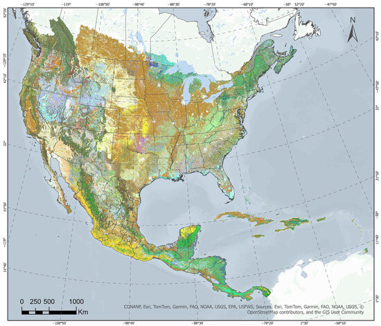
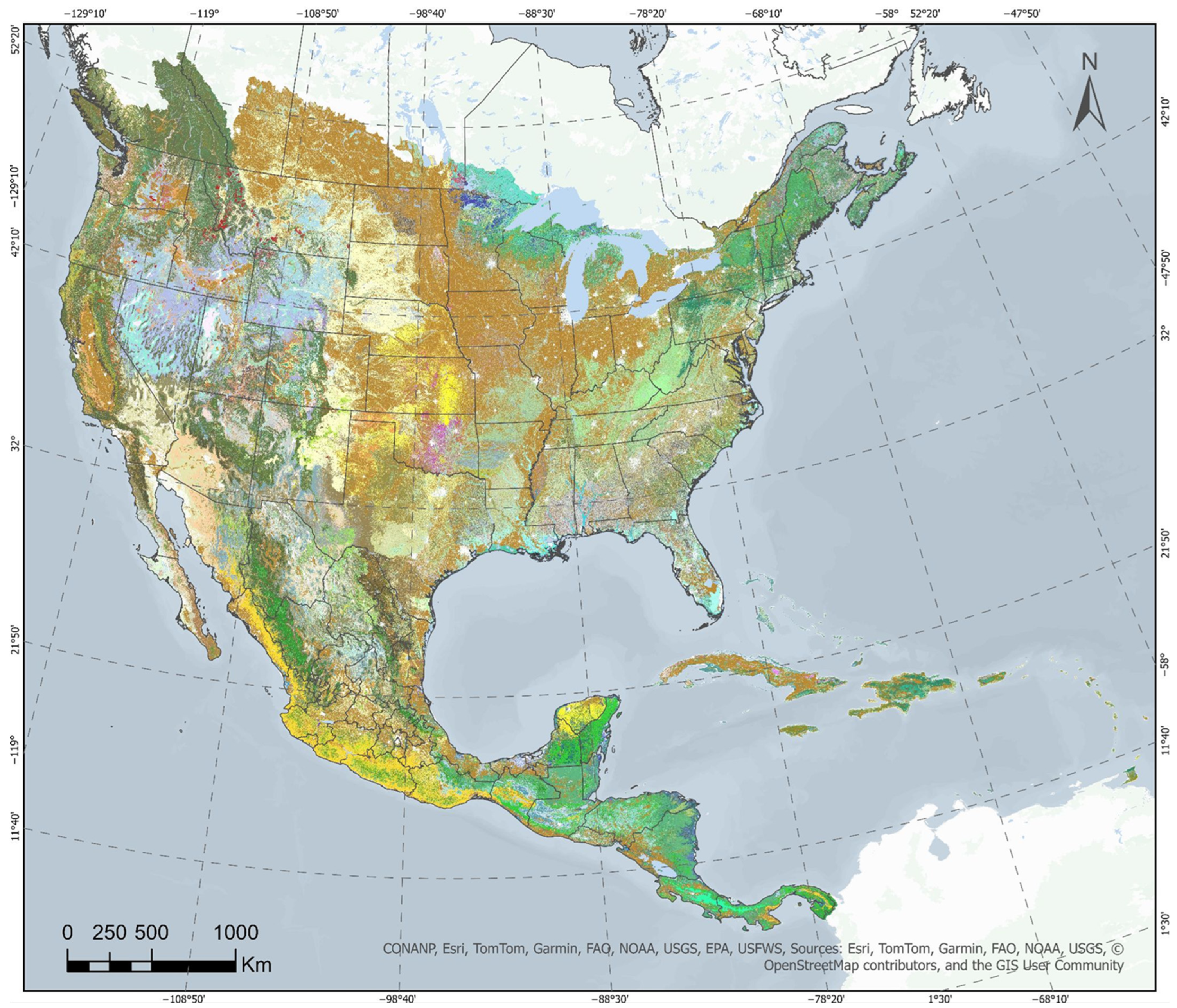
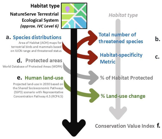
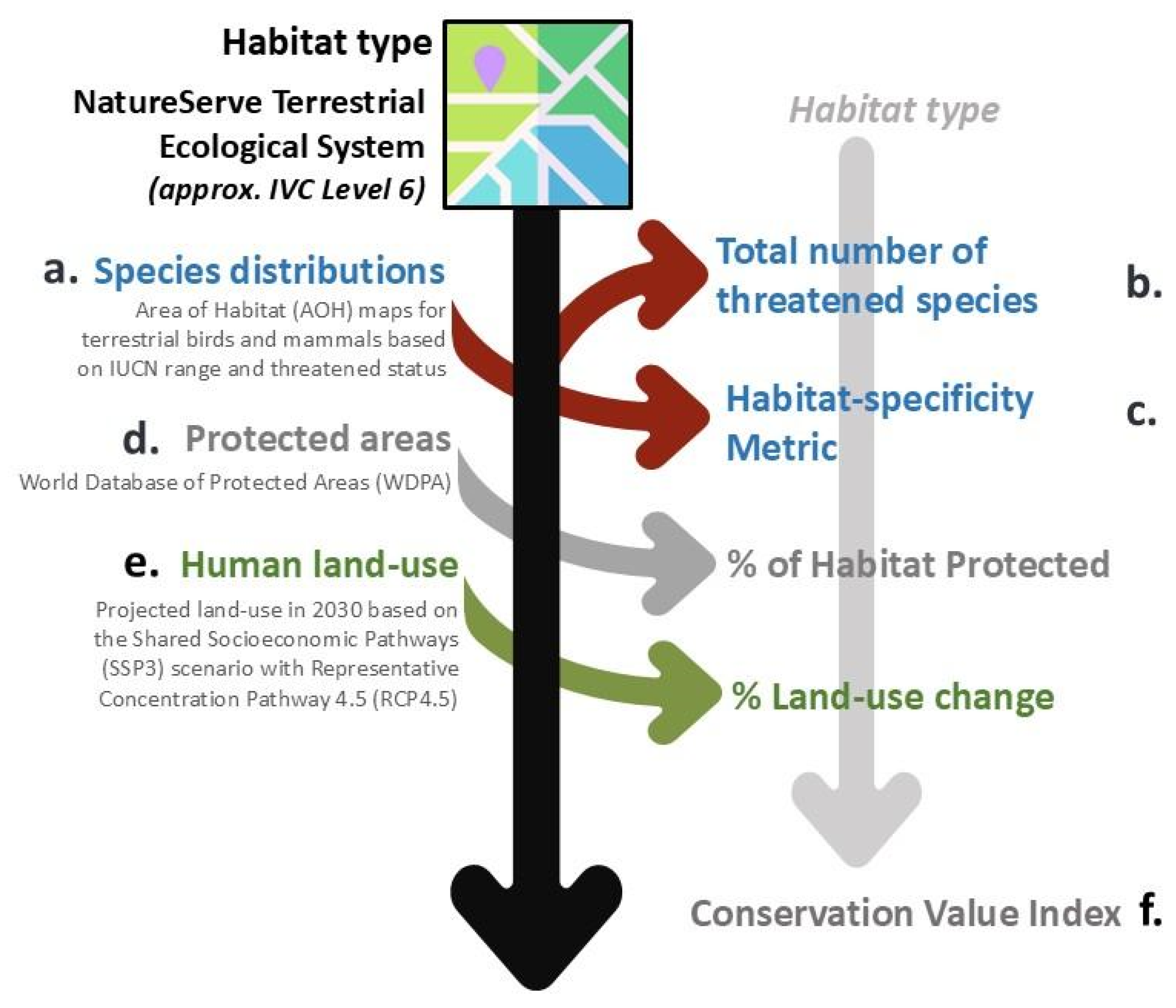
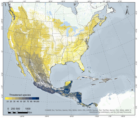
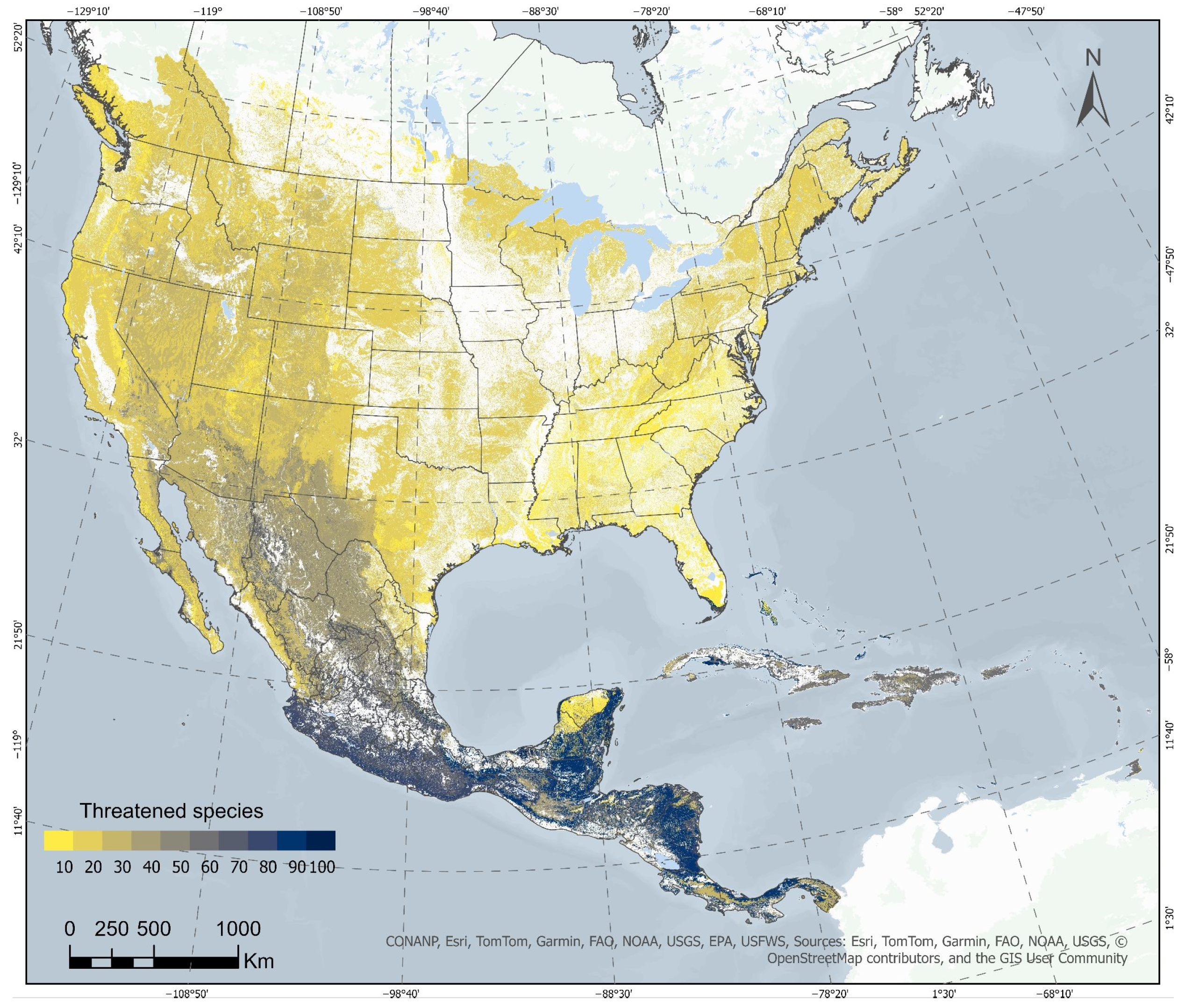
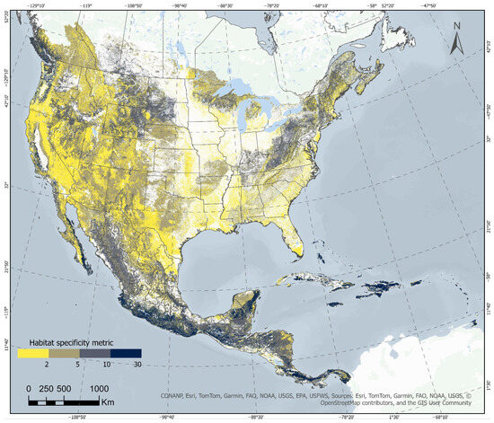
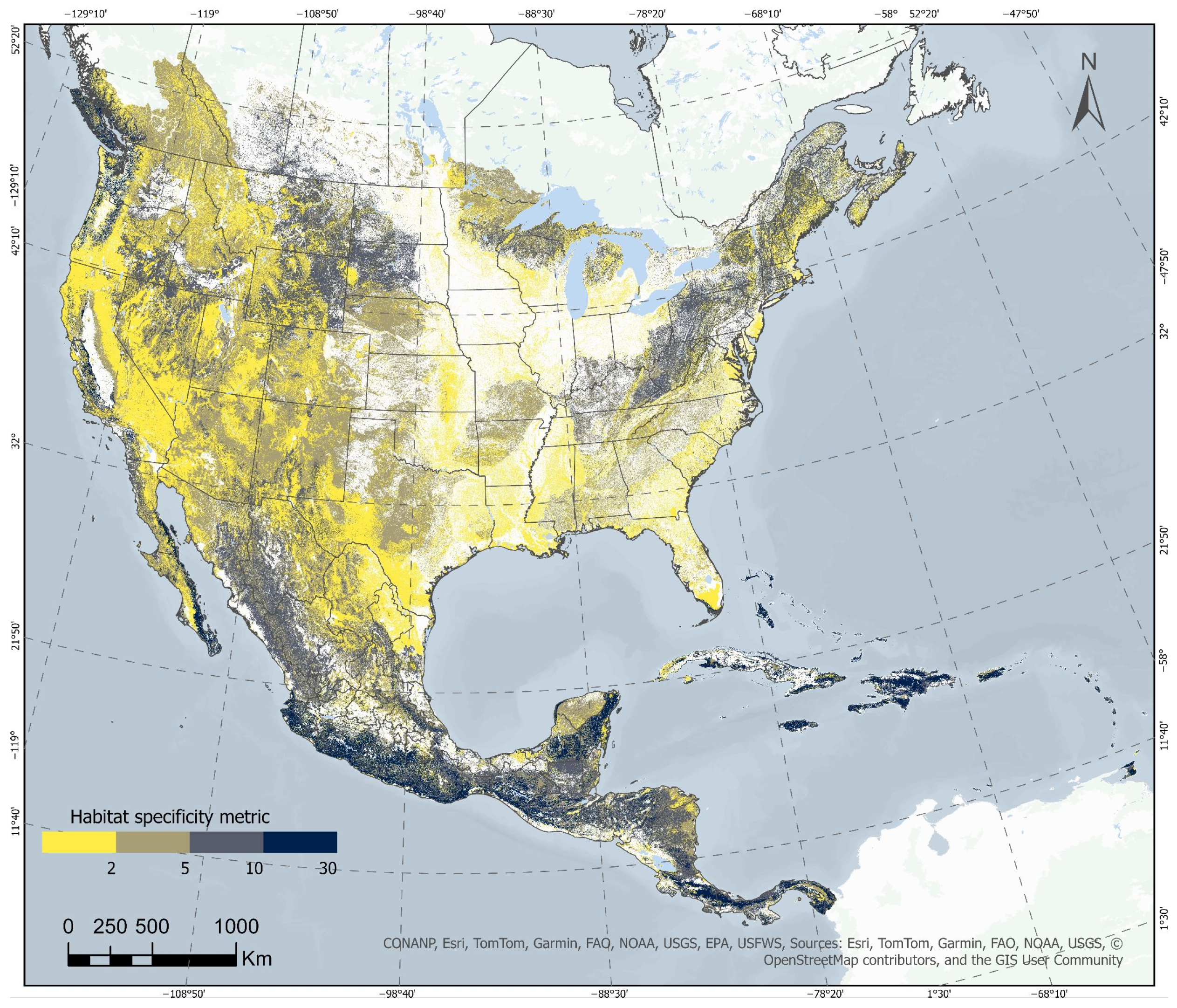
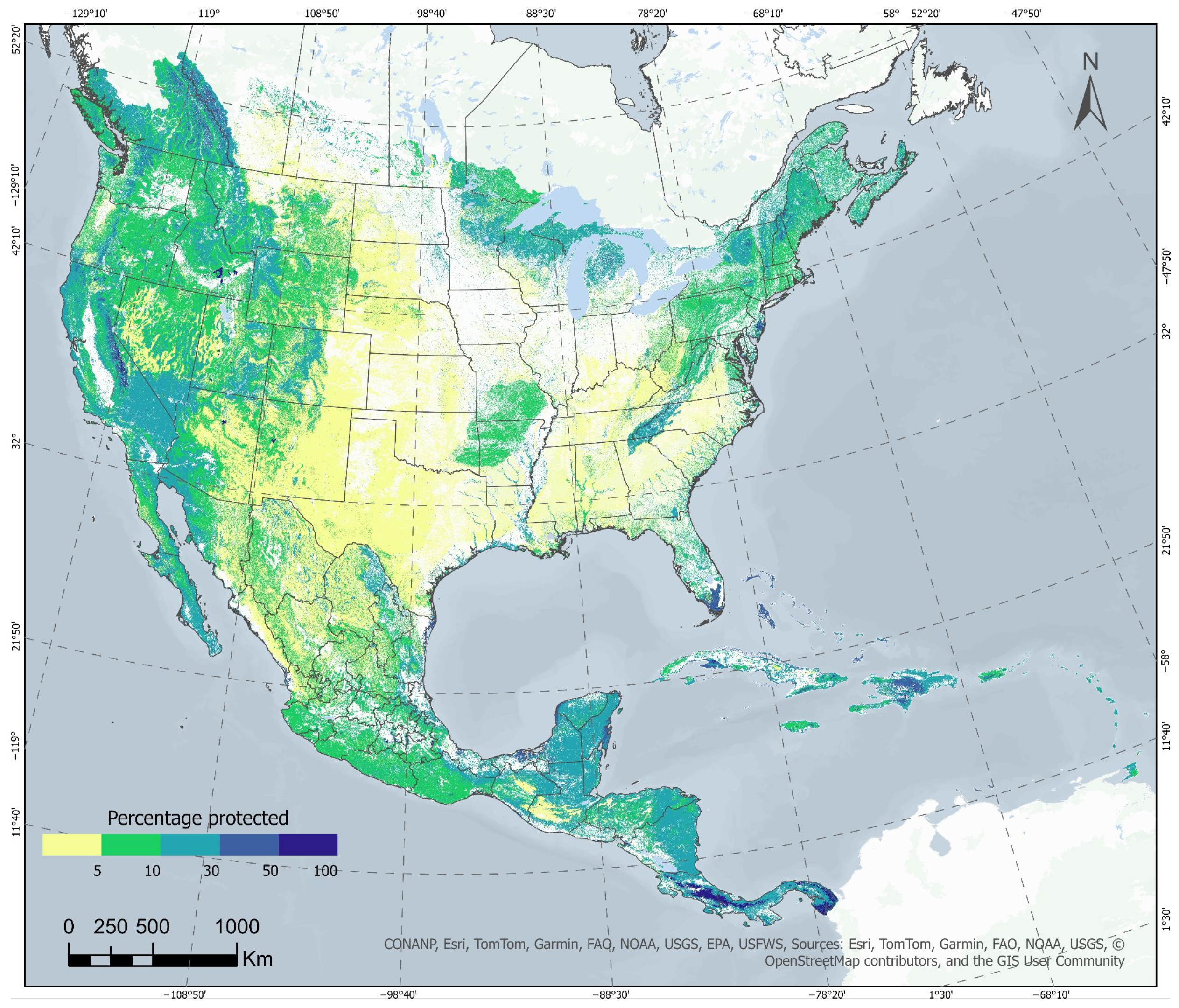
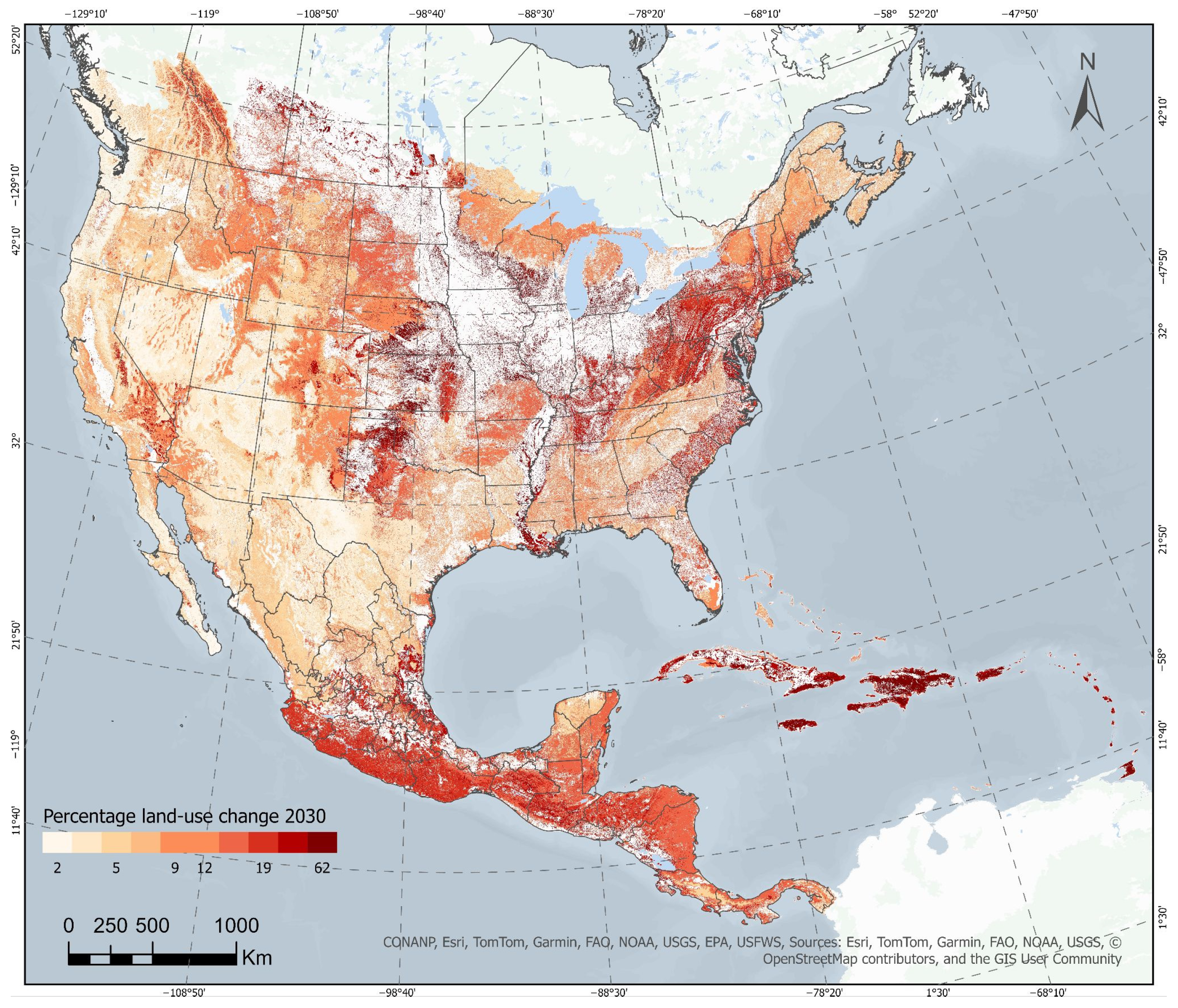
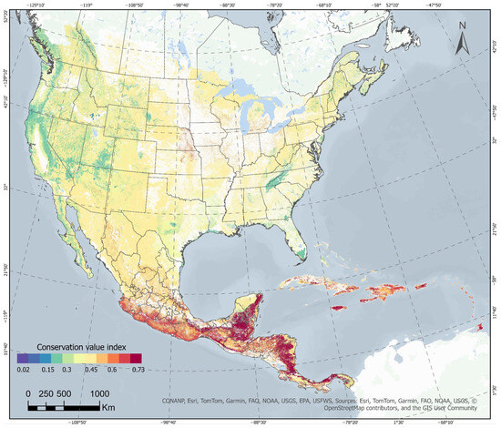
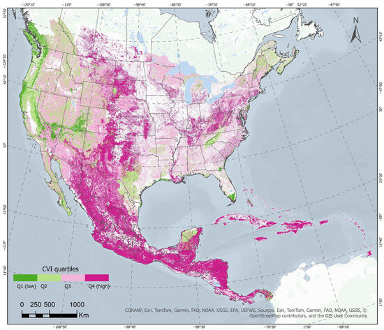
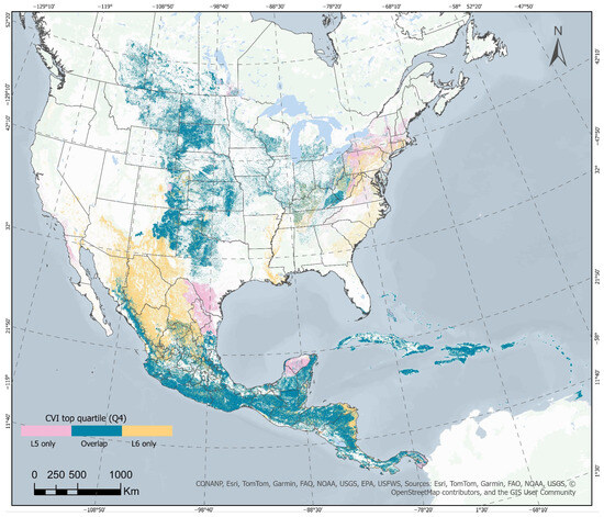
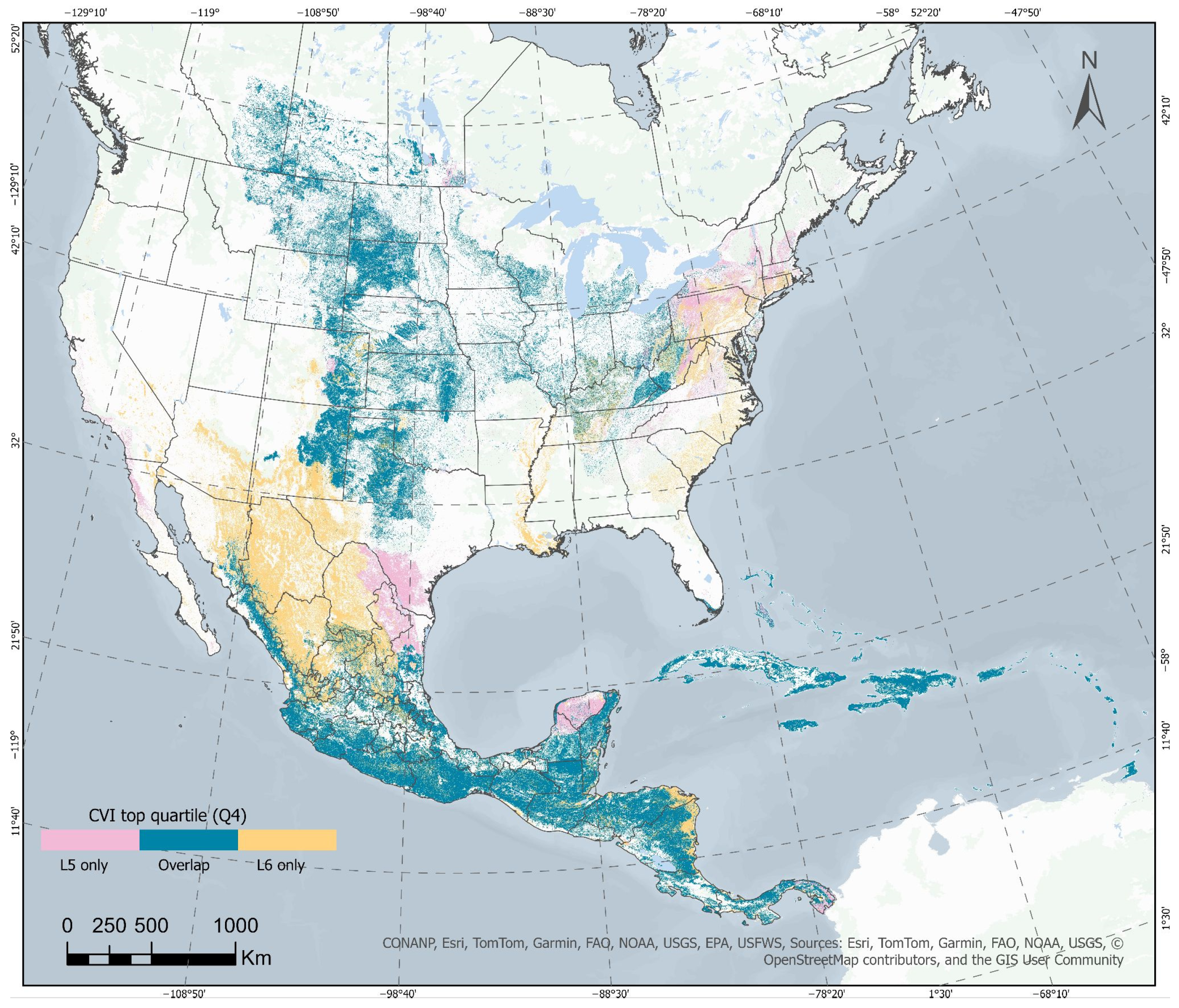
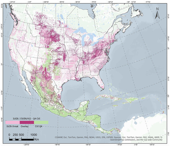
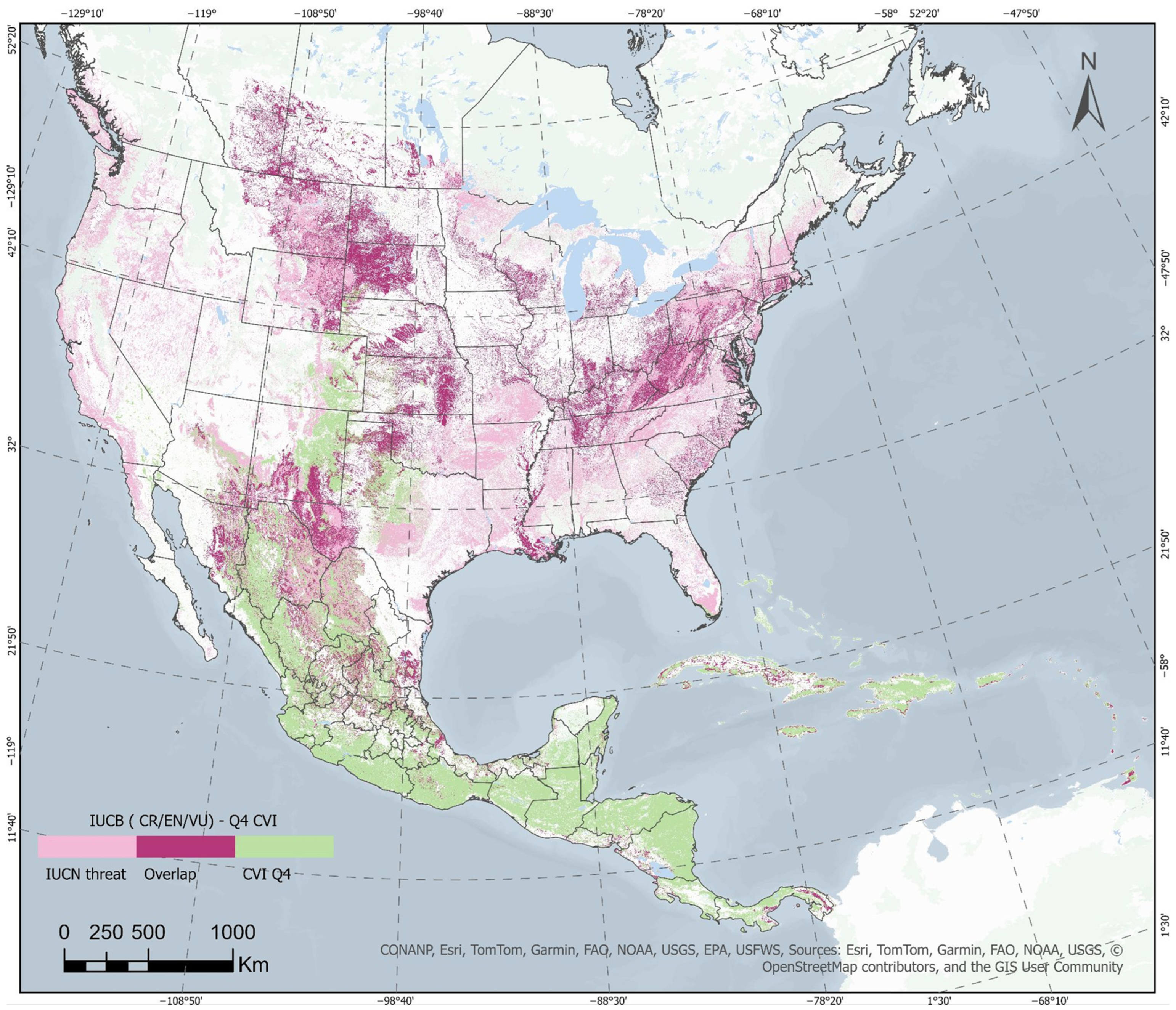

Disclaimer/Publisher’s Note: The statements, opinions and data contained in all publications are solely those of the individual author(s) and contributor(s) and not of MDPI and/or the editor(s). MDPI and/or the editor(s) disclaim responsibility for any injury to people or property resulting from any ideas, methods, instructions or products referred to in the content. |
© 2026 by the authors. Licensee MDPI, Basel, Switzerland. This article is an open access article distributed under the terms and conditions of the Creative Commons Attribution (CC BY) license.