


Abstract
The transition towards climate neutrality requires the development of spatially explicit planning approaches that account for territorial differences and land-use dynamics. Within this conceptual framework, this study has the objective of identifying and discussing spatially explicit planning approaches that can support the transition to climate neutrality in different regional spatial contexts. With reference to this research question, a methodological framework is introduced and applied that is designed to support climate neutrality through spatial planning strategies. Carbon sequestration (CS) serves as a key metric to evaluate both the current state and the temporal evolution of this process, examined in connection with the provision of specific ecosystem services (ESs) within the relevant spatial setting. The work is structured as follows. An approach is developed to define the provision of ESs. Drawing on previous research and detailed assessments of environmental, landscape, and socio-cultural features, the study considers the following ESs: maintaining or improving habitat quality to sustain the life cycles of wild species valuable to humans; regulating climate by mitigating land surface temperature; agricultural and forestry production; and nature-based recreational opportunities. Moreover, spatial relationships between CS capacity and ES provision are examined through geographically weighted regressions, allowing comparisons across Basilicata, Campania, and Sardinia, three Regions in southern Italy forming the Italian Mezzogiorno. The multifunctional characteristics of ES supply contributes to optimizing CS capacity and advancing climate neutrality goals. In particular, in all three regional contexts, high values of CS capacity elasticity are recognized in relation to habitat quality and ground temperature mitigation, and very low elasticity conditions as regards the supply of recreational ESs and agricultural and forestry production.
1. Introduction
Climate change (CC) currently represents one of the most significant challenges to global stability, increasingly affecting both rural and urban environments by compromising human health, physical well-being, and overall quality of life [1]. The evident consequences of global warming necessitate urgent and decisive action to meet the targets established by the Paris Agreement, which seeks to limit the temperature increase to 1.5 °C above pre-industrial levels. Achieving this objective requires a long-term balance between greenhouse gas emissions and removals, a pursuit often referred to as climate neutrality. This task is made more arduous by the persistence of carbon dioxide (CO2) in the atmosphere; even if all human-induced emissions were to cease immediately, existing concentrations are projected to cause an additional warming of approximately 0.6 °C over the next one hundred years [2]. Consequently, the European Union (EU) has formalized its commitment through the European Climate Act, the Green Deal, and the “Ready for 55” package, targeting a 55% reduction in emissions by 2030 and full climate neutrality by 2050.
Human activities, particularly the combustion of fossil fuels and extensive land clearing, have fundamentally disrupted the global carbon cycle. Currently, anthropogenic activities influence over 70% of the Earth’s ice-free land surface, utilizing a third of its potential biological productivity. In the Italian context, this pressure is manifest in increasing land consumption and urban sprawl, which have led to biodiversity loss and heightened environmental risks such as floods and heat islands [3,4].
Within this framework, regulating ecosystem services (ESs), specifically Carbon Capture and Storage (CCAS), are vital for mitigation and adaptation. CCAS is a natural phenomenon, primarily driven by photosynthesis, through which terrestrial ecosystems remove CO2 from the atmosphere and store it in biomass and soil [5]. Soil, in particular, constitutes the largest terrestrial carbon pool; the quantity of carbon locked within the soil is significantly greater than that in above-ground biomass [6]. Therefore, even minor fluctuations in soil organic carbon concentration can exert a substantial impact on atmospheric CO2 levels [7].
Natural ecosystems provide a multifunctional supply of services that interact in complex ways. While the principle of multifunctionality suggests that a single area can provide multiple benefits, certain functions may be mutually conflicting, leading to trade-offs where the enhancement of one service (e.g., carbon storage) may negatively affect another (e.g., biodiversity or agricultural production). Conversely, synergies occur when multiple services improve simultaneously.
Multiple studies document trade-offs and synergies between CCAS and other services. Früh-Müller et al. [8] mapped carbon storage alongside timber supply, crop production, and outdoor recreation across two German counties, Wetterau and Vogelsberg, finding positive relationships among these services except where food production created trade-offs. Bateman et al. [9] quantified land-use conflicts between agriculture, carbon sequestration, recreation, and biodiversity across the UK, demonstrating that targeted planning can increase overall ecosystem service values. Viglizzo et al. [10] provides a comprehensive regression-based analysis, using both parametric and non-parametric regression to examine how carbon sequestration partitions with water-flow regulation, soil protection, and climate regulation across 1348 studies. On the other hand, although regression analysis is a method used by several studies in order to analyze relationships among multiple ESs [10,11], these relationships are analyzed in a stationary way. This study seeks to go beyond the limitations of stationary regression analysis by studying non-stationary relationships in Mediterranean landscapes using a geographically weighted regression (GWR).
From this perspective, this work aims to analyzes the relationship between CCAS and multiple ESs, such as habitat quality, land surface temperature mitigation, agricultural and forestry production, and nature-based outdoor activity potential using a GWR model, in order to determine and critically examine geographically delineated planning methodologies capable of facilitating the progression toward climate neutrality across heterogeneous regional territorial configurations. A GWR-based approach is preferred over ordinary regression models in ES studies for its ability to handle spatial non-stationarity, where relationships vary across locations. ESs like CCAS exhibit spatial variability due to factors such as land use, topography, and climate. Moreover, the correlations are identified in heuristic terms and may form the basis for future studies aimed at identifying causal links between the CCAS supply and the supply of the various ecosystem services considered. This in-depth analysis should be considered an important future development of the research based on the results described and discussed in this study, which show, through the implementation of a GWR-based approach, that there is statistically significant evidence of the existence of these correlations.
The work presents and implements an integrated methodological framework aimed at promoting climate neutrality through spatially oriented planning policies. CCAS is employed as a central indicator to assess both the existing conditions and the dynamic progression of sequestration processes, analyzed in relation to the supply of selected ESs. The methodological approach is structured into two main steps. In the first step, the provision of multiple ESs is assessed. In particular, the study focuses on the following four ESs: maintaining or improving habitat quality to sustain the life cycles of wild species valuable to humans; regulating climate by mitigating land surface temperature; agricultural and forestry production; nature-based recreational opportunities. Each ecosystem service is assessed and mapped using different methods. For example, the use of the InVEST (Integrated Valuation of Ecosystem Services) Suite is, in this conceptual framework, exclusively aimed at identifying, in direct and clear terms, the extent of CCSA provision and habitat quality. In the second part, the spatial interdependencies between CS potential and ES distribution are investigated using a GWR model, enabling comparative analyses among Basilicata, Campania, and Sardinia, three regions located in southern Italy that collectively constitute the Italian Mezzogiorno.
The paper is structured as follows. Section 2 describes the contexts of the three regional case studies and the methodologies used to evaluate and map the selected ESs and for implementing the GWR. Section 3 presents the results obtained, which are then discussed in Section 4. Finally, Section 5 concludes with final remarks and future research directions.
2. Materials and Methods
2.1. Study Area
The study area comprises three regions of the Italian “Mezzogiorno”: Basilicata, Campania, and Sardinia (Figure 1).
Figure 1.
Study areas: Sardinia (panel A), Basilicata, and Campania (panel B).
Basilicata covers an area of approximately 10,000 km2 [12]. The region is predominantly hilly, with plains accounting for about 10 percent of the surface and mainly concentrated along the Ionian coastline, and its landscape is predominantly agricultural, with extensive farming practices and high biodiversity [13]. Mountain ranges are mainly located to the west and include Mount Pollino and the Vulture volcanic complex [14]. The main watercourses, characterized by a predominantly torrential regime, flow into the Ionian Sea and include Bradano, Basento, and part of the Ofanto River. Concerning land covers, according to the latest CORINE data [15], around 57 percent of the region is agricultural, around 41 percent is covered by forests and semi-natural vegetation, and only 1.6 percent is artificial. As of 1 January 2025, 530,005 people [16] lived in Basilicata’s 131 municipalities, of which the main important are Potenza and Matera, the latter being a designated UNESCO site [17].
Campania extends over approximately 13,700 km2 [12]. The regional territory is mainly hilly and mountainous, while alluvial plains account for about 14 percent of the surface. The main mountain systems include the Matese Mountains and the Cilento Massif. Volcanic landforms are a distinctive feature of the region, with two major active volcanoes: Vesuvius and the Campi Flegrei–Ischia volcanic district [18]. The main watercourses are the Volturno and Sele rivers, which exhibit a predominantly torrential regime. Concerning land covers, according to the latest CORINE data [15], around 55 percent of the region is agricultural, around 37 percent is covered by forests and semi-natural vegetation, and 7.5 percent is artificial. As of 1 January 2025, 5,582,337 people [16] lived in Campania’s 553 municipalities, of which the most important are Avellino, Benevento, Caserta, Salerno, and Naples.
Sardinia is the second-largest island in the Mediterranean Sea and has a landmass of approximately 24,000 km2. The regional territory is predominantly hilly and characterized by numerous isolated mountain groups, including Gennargentu, Sette Fratelli, and Limbara [19]. The island’s geomorphology reflects a complex volcanic history and diverse lithological formations [20], and distinctive granite landscapes, particularly to the north of the island, shape unique landforms including inselbergs and tors [21]. Watercourses exhibit a marked torrential regime due to the characteristics of the terrain, dry summers, and limited rainfall [19], and coastal wetlands constitute a distinctive landscape feature. Concerning land covers, according to the latest CORINE data [15], around 46 percent of the region is agricultural, around 50 percent is covered by forests and semi-natural vegetation, and only 3 percent is classed artificial. As of 1 January 2025, 1,562,381 people [16] lived in Sardinia’s 377 municipalities, of which the most important are Cagliari and Sassari.
2.2. Carbon Capture and Storage
We assess carbon capture and storage (CCAS) assessed using the InVEST Suite, which quantifies overall carbon sequestration by integrating four distinct carbon pools: living biomass located both above the surface (aboveground biomass) and in subsurface layers (belowground biomass, confined to the upper 30 cm of the soil profile), dead organic material, and soil organic matter. According to the InVEST User Guide, aboveground biomass (AGB) encompasses all living vegetation located above the soil surface, including structural and foliar components such as stems, bark, branches, and foliage. In contrast, belowground biomass (BGB) refers to the living root systems associated with aboveground vegetation. Dead organic material includes both surface litter and woody debris, whether standing or downed. Lastly, soil organic matter, constituting the largest pool of terrestrial carbon, comprises the organic constituents embedded within the soil matrix [22].
The InVEST Model requires only two inputs: a land cover map and a table in .CSV format showing carbon density values corresponding to the classes in the land cover map. The table should have the density values for at least one of the four pools. We utilize Corine Land Cover (CLC) 2018 as the land cover map. The information on the carbon density values for different carbon pools is sourced from various data sources such as NASA’S ORNL DAAC [23], used for aboveground biomass and belowground biomass, National Inventory of Forests and Carbon Pools in Italy [24,25], used for dead organic material and soil organic matter, ISPRA (Italian Institute for Environmental Protection and Research) [26], used for soil organic matter, and AGRIS Sardegna (Regional Agency for Agricultural Research of Sardinia) [27], used for soil organic matter.
The methodology is implemented in two stages. First, we upload to InVEST information on three pools except belowground biomass. Then, we overlay the result with the ORNL DAAC BGB map, as data for BGB was sourced from this single map; therefore, we integrated it as a separate step by summing cell by cell the values of the ORNL DAAC BGB map and the map related to the three pools using the “Raster calculator” tool in ArcGIS. The decision to use the sum reflects the methodological approach used by InVEST to calculate the value of the final map. In fact, InVEST adds up the values for the three different pools to obtain the final values.
2.3. Habitat Quality
We assessed habitat quality (HQ) using the InVEST Habitat Quality Model, which requires four key inputs: a land cover map, a directory containing threat maps, a sensitivity table, and a threats table. We adopted threats from the study by Sallustio et al. [28], which identifies the following:
- Roads 1: Motorways; trunks; primary roads;
- Roads 2: Secondary and tertiary roads;
- Roads 3: Residential and service roads;
- Roads 4: Tracks and bridleways;
- Railways;
- Intensive agricultural lands;
- Extensive agricultural lands;
- Buildings and other artificial areas or impervious soils.
Threat maps were generated using the Geofabrik Download Server [29] and CLC 2018 [15]. The land cover map was derived from the CLC 2018, reclassified into 12 habitat types following the classification by Sallustio et al. [28]:
- Beaches, dunes, and sands
- Water bodies
- Wetlands
- Grasslands
- Shrublands
- Broadleaves forests
- Conifers forests
- Inland unvegetated or sparsely vegetated areas
- Intensive agricultural lands
- Extensive agricultural lands
- Buildings and other artificial areas or impervious soils
- Open urban areas
In the case of Sardinia, we introduced the additional habitat type “mixed forest” to reflect local characteristics.
The sensitivity table details how each habitat responds to the defined threats. The average values of “broadleaves forests” and “conifers forests” were utilized for the “mixed forest” category.
The threats table provides three parameters: MAX_DIST, the maximum distance at which each threat impacts HQ; WEIGHT, the relative weight of each threat compared to other threats; and DECAY, the spatial decay function of each threat. We assumed the decay parameter as linear in this study as there are no available data supporting alternative functions.
The model integrates these inputs to calculate the HQ scores using a degradation equation, which employs the half-saturation constant (K) to calibrate the spread and variation of scores along the 0–1 scale. K selection directly affects the absolute HQ scores, which serve as key inputs for the GWR analysis and therefore influence the scale of the resulting outputs. To maximize visual contrast, we performed a preliminary run with the default K = 0.05 to identify the maximum degradation value; we the adjusted K to half this value for the final run, following recommendations in the InVEST model’s user guide [30], consistently with previous applications [31,32,33]. The final output is a continuous gradient map that illustrates the spatial distribution of HQ.
2.4. Regulating Local Climate: Land Surface Temperature Mitigation
We assessed the Land Surface Temperature (LST) using satellite images provided by USGS Earth Explorer [34]. First, the images from the specified date range were downloaded for selection, which was set from the last week of June to the first week of September to cover the summer season to capture the highest average temperatures in each of the three study areas. The maximum cloud cover was set to a 6%. All downloaded images were analyzed further to identify the one with the highest median LST. In all cases considered, i.e., five Landsat images selected for Sardinia, four selected for Campania, and one selected for Basilicata, the selection of images is such that those with the highest median coincide with those with the highest means. To do so, the digital number (DN) values in the raster image were converted into degree Celsius (°C) by using the formula (1), as per the USGS guide [35].
0.00341802 ∗ DN + 149.0 − 273.15,
Depending on the research area, one or more satellite pictures may be necessary to encompass the entire region. Table 1 shows the full set of images utilized to create an LST map for the three regions. It is important to note that temporal variability in temperature measurement may lead to minor inconsistencies. This limitation is absent for the Basilicata Region, where LST is derived from a single image (Table 1), whereas for Campania and Sardinia full regional coverage is obtained by combining multiple LANDSAT images as indicated in Table 1.
Table 1.
Selected Landsat images to create an LST map for Basilicata, Campania, and Sardinia Regions.
2.5. Agricultural and Forestry Production
We classified agricultural and forestry production among provisioning ESs, a category that encompasses material goods such as food, freshwater, timber, fiber, and energy resources. Recognized by the Millennium Ecosystem Assessment [36], provisioning ESs represent a fundamental component of sustainable land management, particularly in regions characterized by high landscape heterogeneity and extensive agro-forestry systems, as is the case in Italy. In recent years, also in response to the reforms of the European Common Agricultural Policy [37] and international frameworks on climate and sustainable development, the economic valuation of provisioning ESs has increasingly been incorporated into land-use planning and strategic environmental assessment.
In the three regions analyzed, the evaluation of the value of agricultural and forestry production (AFPL) relies on the market value on the production related to land uses, as a proxy indicator based on geographic and environmental variables such as location, altitude, morphology, and orography. This methodological approach, consolidated in recent studies, employs two primary datasets: (i) the national agricultural land value database produced by the Council for Agricultural Research and Economics (CREA), which provides average monetary values per unit area for agricultural lands; (ii) the dataset issued by the National Revenue Agency (NRA) reporting mean land values for forestry areas. Information on agrarian and forestry regions, organized by municipality, province, and elevation zone, enables detailed spatial analyses [38]. To integrate the datasets, correspondence was established between the CLC 2018 classes, and the crop typologies identified by CREA for agricultural land, as well as the NRA’s taxonomy for forest land. The resulting data were combined through spatial overlay of the land-cover vector map with the agro-forestry value map, allowing the assignment of production values to each classified spatial unit.
2.6. Nature-Based Outdoor Activity Potential
We conducted the assessment of nature-based outdoor activity potential using the ESTIMAP (Ecosystem Service Mapping Tool) methodology, a GIS-based framework, developed by the Joint Research Centre (JRC) [39]. The study specifically implements the first part of the original model developed by Vallecillo et al. [40], Barton et al. [41], and Isola et al. [42] to quantify the recreational potential, defined as the capacity of ecosystems to support nature-based outdoor activities. We structured the methodological approach into three distinct phases. The first phase evaluates the availability of recreational areas based on their degree of naturalness. Central to this assessment is the hemeroby index, which measures the divergence of an ecosystem from its natural state due to human intervention on a scale from zero (no modification) to nine (maximum modification) [43]. For agricultural land, we determined the index by cross-referencing nitrogen nutrient inputs (utilizing ISTAT data from 2019 for Sardinia, and 2023 for Basilicata and Campania) and livestock density measured in Livestock Units (LSU) [44]. Forested areas are qualitatively assessed by comparing current land cover with potential natural vegetation maps to determine the level of disturbance [43]. The final values are inverted and normalized into a 0–1 range, where 1 represents maximum naturalness. The second phase integrates the presence of recreationally significant natural features, such as national and regional parks, Ramsar sites, and Natura 2000 sites. Scores are expert-based and attributed according to IUCN management categories, resulting in a raster map with discrete values [0; 0.8; 1] representing the legal and environmental significance of the land [39,45]. The final phase focuses on the attractiveness of coastal zones through three parameters: (i) distance from the coastline, modeled via an inverse logistic function; (ii) coastal geomorphology, using the Eurosion dataset [46]; and, (iii) bathing water quality, based on European Bathing Water Directive data [47]. We calculated the total potential supply of nature-based outdoor activity potential by summing the normalized outputs of all three phases, providing a comprehensive spatial representation of recreational potential for outdoor activities across the diverse topographies of Basilicata, Campania, and Sardinia.
2.7. Geographically-Weighted Regressions
We investigated the relationship between CCAS capacity and the supply of the four ESs selected for the study proposed here using a GWR model, according to the formalization proposed by [48], which is briefly described below.
The model provides information on how the dependent variable, representing CCAS, is associated with the explanatory variables, which express the supply of ESs, when the relationship is not spatially stationary and, therefore, presents a more or less pronounced variability across the territory.
We formalize the spatially stationary multiple linear regression according to the following formulation, in which the coefficients of the explanatory variables are considered constant in the spatial context of reference, therefore, in our case, in the three regional study areas: Basilicata, Campania, and Sardinia:
where (units of measurement in parentheses):
CCAS = a0 + a1 LOHM + a2 QOHA + a3 AFPL + a4 NOAP,
- CCAS is the density of carbon capture and storage capacity (Mg/m2);
- LOHM is the heat mitigation reference, i.e., the land surface temperature (LST), which serves as a measure of urban heat fluctuation and, consequently, to assess changes; if it were to decrease, it would indicate an improvement in the quality of life for users of local environments (°C);
- QOHA measures the level of habitat quality, and takes values ranging from 0 and 1, as described in Section 2.3;
- AFPL is the value of agricultural and timber production (€/ha);
- NOAP measures the potential for nature-based outdoor activities, and takes values ranging from 0 to 1, as described in Section 2.6.
The estimated coefficients of the explanatory variables show the marginal impacts of these covariates on the CCAS. The regression model is typically used when no prior assumptions can be made about the functional relationships between the variables [49,50,51,52].
The linear regression operationalizes the equation of a hyperplane, which is tangent to a hypersurface of an unknown shape within an n-dimensional hyperspace that includes the dependent variable CCAS, together with four explanatory variables. Near the point of tangency, the linear correlations between the five factors, which come from the estimation of model (2), effectively approximate the unknown equation of the hypersurface of unknown shape mentioned above [53,54].
Significance tests for the estimated coefficients are usually assessed using p-values, and the adjusted R-squared is the reference for evaluating the goodness of fit.
The GWRs model replaces the linear regression model when, as in the case of the three regions considered in this study, there is a large number of records, in our case tens of thousands, located in a vast and non-homogeneous territory, such as the regions of Basilicata, Campania, and Sardinia. In this case, the linear relationship between the variables, expressed by model (2), is not stationary in the spatial contexts of reference, but varies with location point, which corresponds to one of the thousands of records, in which it is estimated.
The GWRs model proposed by [48], therefore, estimates a cloud of multiple linear regressions represented by the following formulation:
where xi and yi represent the geographical coordinates, in the regional territories of Basilicata, Campania, and Sardinia, of the various records represented by quintuples of values of the dependent variable and explanatory variables.
CCAS(xi,yi) = α0 (xi,yi) + α1 (xi,yi) LOHM + α2 (xi,yi) QOHA + α3 (xi,yi) AFPL + α4 (xi,yi) NOAP,
For each of the points where the records of the three spatial contexts are located, we implement the regression estimate (3) by assuming a decay function of the influence of the explanatory variables on the dependent variable, according to which this influence decreases as the distance of the point (xi,yi), where the i-th record is located and where the i-th GWR is estimated, increases. We express the decay function, as a function of distance, according to the Gaussian weighting scheme [48], using a weight wij, according to the following formula:
where wij is the weight of the j-th record, located at the point with coordinates (xj, yj) at a Euclidean distance dij from the point with coordinates (xi, yi), where the i-th record is located, with respect to whose location the i-th GWR is being estimated. Formulation (4) is such that: (i) wij = 1 when the record (xj, yj) coincides with the one detected at the point with coordinates (xi, yi), with respect to which the i-th GWR is estimated; (ii) wij decreases exponentially as the distance of the point (xj, yj) from the point (xi, yi) increases; (iii) records located at a distance dij greater than some multiple of b have a progressively reduced influence in the estimation of the GWR estimated with reference to the point (xi, yi).
wij = exp[−(dij/b)2],
According to the detailed and analytical discussion of the model proposed by [48], the value of b, called bandwidth, must be chosen in such a way as to bear in mind that there is a trade-off in terms of unbiasedness and reliability of the GWR estimate. This trade-off must be considered when choosing the bandwidth, which defines the decay function, and therefore the weight wij to be assigned to the records based on their distance from the point at which the GWR is estimated.
On the one hand, the smaller the bandwidth, i.e., the faster the weight wij decreases with increasing distance dij, the more records become irrelevant and are therefore essentially excluded from the GWR estimate. Thus, the smaller the bandwidth, the higher the biasedness of the biased estimator of the variable CCAS(xi, yi), expressed by model (3).
On the other hand, the larger the bandwidth, the more records are included in the GWR estimate. Therefore, in this case, although the bias decreases, the variance of the biased estimator of the variable CCAS(xi, yi) of model (3) is greater.
It is therefore very important, for the purposes of applying the GWRs model, to identify the bandwidth in such a way as to find the best compromise between minimizing the variance and the bias of the estimate of the dependent variable CCAS(xi, yi).
As suggested by [48], the choice of the bandwidth measure is defined by the solution to the following problem of minimizing the variance of the CCAS(xi, yi) estimate.
The minimization problem is operationalized as follows, with reference to the GWR estimate at the coordinate point (xi, yi), where the i-th record is located:
minb ∑i = 1,n (Yi − Ŷi)2,
In our case, Yi corresponds to the value of the dependent variable CCAS(xi,yi) relative to the i-th record, and Ŷi is the estimate of the variable based on the implementation of GWRs, determined using the estimates of the coefficients αj, âj, j = 0, … 4, of (2).
The estimates âj’s are defined by the following matrix formula [48]:
where
â(xi,yi,b) = [XT W(xi,yi,b) X]−1 XT W(xi,yi,b) Y,
- â(xi,yi) is the vector of the estimates of the α’s coefficients of (3);
- X is the matrix (n × 5) of the n records related to the constant and the four explanatory variables of (3);
- W is the diagonal matrix (n × n) whose diagonal elements represent the weights of the n records representing the observations relating to the explanatory variables; the n weight values are defined by formula (4);
- Y is the vector of n observations relating to the dependent variable CCAS(xi,yi).
The estimates âj, j = 0, … 4, derived from (6), allow us to express, in (5), Ŷi, i.e., the estimate of Yi, value of the dependent variable of the record detected in the location (xi,yi), using (3) and, therefore, to solve, in b, the minimization problem (5). The search for the value of the bandwidth b that solves the minimization problem (5) can be carried out, as suggested by [48], by applying the golden section share algorithm described by [55], with reference to the field defined by the minimum and maximum distances of the locations of the records detected.
With regard to the goodness-of-fit of the GWRs estimate, the following statistics are important: (i) the adjusted R-squared or adjusted coefficient of determination, which measures the share of the overall variance of the phenomenon represented by the dependent variable, in our case the CCAS, explained by the GWRs estimate, purifying this measurement from the increase in the coefficient linked to the number of explanatory variables; (ii) the adjusted critical value of pseudo-t statistics, which is used to verify the statistical significance of the estimated coefficients using a two-tailed t-test, at a significance level of 5%; this test takes into account the degree of freedom of the estimate and checks in relation to the family-wise error rate (FWER).
The spatial distribution of the vector â(xi,yi), which derives from the GWRs estimate, locally characterizes the correlations between the dependent variable CCAS(xi,yi) and the four explanatory variables that express the availability of the four ESs.
The methodology described above, based on the aforementioned seminal article by Fotheringham et al. [48], has been applied in the field of analysis relating to the spatial profiles of ES supply. The following are some examples of these studies. Shi and Xu [56] analyze the distribution of ESs in an urban green space system in the coastal metropolis of Suzhou, Jiangsu Province, China, through the integrated use of the InVEST suite, machine learning techniques, and the GWR approach, in relation to the spatial heterogeneity of ES supply. Another very interesting study is that of Neill et al. [57], which applies a spatial analysis based on GWRs to examine the relationship between environmental indicators and cultural ecosystem services in multiple sites in Europe, with the aim of bypassing the limitations of models that do not take into account the non-stationarity of ES supply.
3. Results
3.1. Carbon Capture and Storage
The CCAS taxonomy is intrinsically linked to the biophysical characteristics of the territory, with particular reference to land cover, especially in relation to forest types. As can be seen below, the spatial distribution of this ES supply shows the highest values in forest-covered soils, albeit with significant differences depending on forest types, while significantly lower values are found where vegetation is lower and sparser, and, above all, in more or less densely built-up areas.
The CCAS assessment yields that in all three regions highest capacity is observed in forests (Figure 2). Campania exhibits the highest density at 23.82 kg/m2, followed by Basilicata at 21.21 kg/m2, both observed in broad-leaved forests, whilst Sardinia’s maximum value is 17.75 kg/m2, noted in the coniferous category. In all three regions, forest ecosystems (CLC 311, 312, 313) represent the primary carbon pool. However, average forest productivity varies significantly. Campania’s forests range from 15.07 to 17.40 kg/m2, followed by Basilicata (12.88–14.76 kg/m2) and Sardinia (10.99–12.65 kg/m2). A notable regional anomaly is identified in Sardinia, where broad-leaved forests consistently store less carbon (10.99 kg/m2) than coniferous or mixed forests across all carbon pools. Spatially, high-density clusters are strongly correlated with mountainous topography and protected areas, such as the Cilento and Vesuvius parks in Campania, the Pollino and Appennino Lucano in Basilicata, and the eastern/southwestern massifs in Sardinia. Intermediate storage levels (7.77–10.54 kg/m2) are found in shrublands and marshes, while artificial areas and water bodies consistently yield the lowest results. Moreover, these regions act as natural reservoirs. Campania serves as a high-capacity tank, Basilicata as a well-distributed network of medium basins, and Sardinia as a specialized reservoir where specific cluster, coniferous forests, are more efficient than others.
Figure 2.
Spatial distribution of the five ecosystem services in the three study areas.
3.2. Habitat Quality
The analysis of HQ shows consistent contrasts between high values characterizing natural areas and low values found in urban and intensive agricultural areas. Human infrastructures are recognized as major sources of degradation, reducing HQ scores according to their proximity and their threat level.
Sardinia records the highest average HQ (0.54) and the greatest proportion of high-quality habitats (40.86%). Basilicata follows with an average score of 0.51, but with the highest percentage of low-quality habitats (44.45%). Campania reports the lowest average HQ (0.49) and the smallest share of high-quality habitats (31.43%). In all regions, the best habitats are forested areas; broadleaved forests exhibit the highest mean scores (ranging from 0.85 to 0.86), followed by grasslands and wetlands. Conversely, artificial surfaces and impervious areas score near zero (0.09) across all regions, with open urban fabric and intensive arable land also exhibiting very low values (0.21–0.25). Spatial patterns reflect this gradient: high values cluster in national and regional parks, such as Pollino and Appennino Lucano in Basilicata, Cilento and Vesuvius in Campania, and Gennargentu, Limbara, and Gutturu Mannu in Sardinia, while low values characterize major urban centers, like Matera, Potenza, Naples, Salerno, and Cagliari, and intensively cultivated plains. Differently, extensive agricultural systems and sparsely vegetated inland areas occupy an intermediate position (0.43–0.53).
The biophysical characteristics of the reference territory, in all three regional cases analyzed, are decisive in identifying the HQ level. First of all, we note that some of these characteristics are decisive in relation to the classification of threats, which are linked to agricultural land use, whether extensive or intensive, or to the degree of soil permeability. This is strongly influenced by the biophysical characteristics of the soil as modified by human activities and, in particular, by the level and type of infrastructure. In this regard, it is worth highlighting the radical difference between threats related to green infrastructure and those related to gray infrastructure, with particular reference to transport infrastructure.
Secondly, we note how the biophysical characteristics of soils come into play, in a structural and pervasive manner, with reference to the assessment of HQ in the InVEST Suite, where these characteristics identify the quality of soil cover through the Corine Land Cover mapping units and their sensitivity to threats in terms of loss of ESs supply capacity.
3.3. Regulating Local Climate: Land Surface Temperature Mitigation
In Campania, LST ranges from about 27.5 to 64.5 °C (Figure 2), with the highest values concentrated in densely urbanized and artificial areas. Hotspots include the Metropolitan City of Naples, the Campanian and Phlegraean plains, the areas in the crown of the Vesuvius Volcano, and agricultural sectors in Avellino, Benevento, and the Sele Plain. Lower temperatures occur along the Apennine ridge, where mountainous and hilly landscapes dominate. CLC data show that artificial fabrics (CLC 111–112) exhibit the highest mean LSTs (47.6–53.3 °C), while water bodies, wetlands, forests, and herbaceous or shrub-covered areas (CLC 512, 521, 311–313, 323–324) display the lowest values (34.3–39.4 °C). Overall, thermal patterns align with land-use intensity, with cooler conditions in vegetated and high-elevation zones.
In Sardinia, LST ranges from around 27.8 to 61.9 °C (Figure 2). The highest temperatures occur mainly in agricultural zones, especially in the eastern sector, while cooler values characterize mountainous, forested, and protected areas such as Limbara, Sulcis-Iglesiente, Gennargentu, and Sette Fratelli. CLC data show that while the highest temperatures are observed in agricultural fields and discontinuous urban fabric (both 61.9 °C), the highest mean values are observed in artificial areas such as construction sites (54.0 °C), dump sites (51.2 °C), and airports (50.1 °C). Water bodies and forests remain the coolest (32–40 °C).
Basilicata’s LST, derived from a single Landsat scene covering the entire region, ranges from 24.1 to 62.5 °C (Figure 2). Higher values occur in industrial, commercial, and agricultural areas of the northeast, including the Bradano basin, Vulture Hills, and the urban zone of Matera, as well as the Metapontino Plain and Ionian coast. Cooler temperatures characterize the Lucanian Apennines. CLC data indicates the highest mean LSTs in irrigated and mixed agriculture and artificial surfaces, and the lowest in water bodies, forests, and rocky areas.
The relationship between the territorial distribution of LST and spatial biophysical characteristics is evident from the above results. For example, the lowest temperatures in Basilicata and Campania are recorded in the Apennine Mountain range, while in Sardinia they are found in the mountainous areas of Sulcis-Iglesiente, Limbara, Sette Fratelli, and Gennargentu. All these areas are also characterized by their proximity to or inclusion of wetlands, waterways, lakes, woods, and forests.
In the three regions, the highest temperatures are consistently found in intensive agricultural areas, in urbanized areas with high building density, and in peri-urban areas characterized by scattered settlements with marked fragmentation of the spatial continuity of permeable soils and habitats. These areas are, in particular, as already partly highlighted: in Basilicata, the Bradano basin, Vulture Hills, and the urban zone of Matera, the Metapontino Plain, and Ionian coast; in Campania, the Phlegraean plains, the areas in the crown of the Vesuvius Volcano, and agricultural sectors in Avellino, Benevento, and the Sele Plain; in Sardinia, the Campidano Plain, the Upper Oristano area, and the south-eastern coast.
3.4. Agricultural and Forestry Production
The 2023 AFPL map for Campania reveals a highly uneven spatial configuration, with values ranging from zero, where no agricultural or forestry classification is present, to a maximum of EUR 82,316/ha (Figure 2). About 22.08% of the region records a null value, while the mean reaches EUR 12,552/ha. Over half of the territory (52.11%) shows values below EUR 10,000/ha, mainly in the eastern mountain sectors of the Campanian Apennines and the Cilento area. The highest AFPL values are concentrated in the coastal hills of Naples and the Sorrento Peninsula, characterized by high-value arable and horticultural production.
A similar distribution emerges in Sardinia, where the 2023 AFPL values range from zero to EUR 34,766/ha (Figure 2). Around 17.41% of the region falls below EUR 1000/ha, with an overall mean of EUR 5091/ha. Values above EUR 10,000/ha are concentrated in fertile plains such as Campidano di Cagliari, Campidano di Oristano, and Nurra, areas typically dedicated to vineyards, orchards, citrus groves, and horticultural crops. Peaks exceeding EUR 30,000/ha occur in the coastal hills of Sarrabus, in the Lower Tirso plain, and in the Campidano of Serrenti.
In Basilicata, AFPL values range from zero to EUR 20,646/ha (Figure 2). Approximately 9.86% of the Region shows a null value, while 11.44% falls below EUR 1000/ha. The average value is EUR 5689/ha. Higher AFPL values, above EUR 20,000/ha, are found in the Metapontino Plain near the river mouths of the Sinni, Agri, Cavone, Basento, and Bradano, where agricultural production is dominated by orchards and vineyards.
Even in the case of agricultural and forestry production, it is clear that supply is closely linked to the biophysical characteristics of the territory in all three regions considered. In all three cases, the highest values are found where there are flat or hilly, arable soils characterized by vegetable crops, olive groves, vineyards, and citrus groves, located in the Metapontino area in Basilicata, in the plain and coastal hills of Naples in Campania, and in Campidano and Nurra in Sardinia.
More than with reference to the characterization of other ESs, in this case the relationship between ES supply and biophysical characterization is almost deterministic. Finally, it should be noted that the values for Campania are significantly higher than those for the other two regions.
3.5. Nature-Based Outdoor Activity Potential
The assessment of nature-based outdoor activity potential in Basilicata, Campania, and Sardinia reveals significant spatial heterogeneity driven by naturalness and coastal proximity. According to the sources, potential values range from 0.1 to 2.8 in Basilicata and 0.1 to 3.0 in Campania, while Sardinia covers the full 0 to 3 scale with a mean of 1.21 (Figure 2). A common geographical trend emerges, represented by high-value clusters predominantly located along coastal strips, such as the Tyrrhenian and Ionian coasts in Basilicata and the Campania coastline, and within mountainous protected areas. Notable inland clusters include the Pollino and Lucanian Apennines National Parks in Basilicata, the Cilento and Vesuvius National Parks in Campania, and the Gennargentu and Supramonte massifs in Sardinia. Statistical analysis of CLC classes confirms that natural and semi-natural areas provide the highest service levels. Specifically, salt marshes (CLC 421), beaches (CLC 331), and water bodies (CLC 512/522) consistently show the highest mean values across all regions. Conversely, the lowest values are systematically associated with anthropized environments, including industrial units, urban fabrics, and intensive agricultural plains like the Volturno in Campania and the Campidano in Sardinia. These results emphasize that nature-based outdoor activity potential is intrinsically linked to environmental conservation and the presence of significant landscape features.
In the case of outdoor recreational potential, the biophysical characteristics of the territory relate, for all three regions, to the spatial taxonomy of the ES offer in a homogeneous and easily recognizable manner.
In all three cases, in fact, there are two profiles that play a fundamental positive role in identifying areas with high recreational potential: coastal areas and protected natural areas. With regard to the latter, the ES offer is very high: in the Pollino and Lucanian Apennines National Parks in Basilicata; in the Cilento and Vesuvius National Parks in Campania; and in Gennargentu and Supramonte in Sardinia. In terms of land cover, the highest recreational potential values are found on sandy beaches, in coastal lagoons, and in water bodies. The lowest values, on the other hand, are generally found on artificial land and, in particular, in urban areas with high building density.
3.6. Geographically Weighted Regressions
To run the GWR, we created a vector layer composed of one-kilometer square polygons arranged in a regular grid. For each polygon, we calculated the average values of CCAS, LOHM, QOHA, AFPL, and NOAP from the ES maps described in Section 3.1, Section 3.2, Section 3.3, Section 3.4, Section 3.5 and Section 3.6 and shown in Figure 2, using zonal statistics.
Prior to the GWR, we performed an ordinary least squares regression to check for global multicollinearity. For all explanatory variables, the Variance Inflation Factor was always lower than four, and therefore well below ten, a commonly used threshold for identifying potentially problematic multicollinearity [58,59,60].
Subsequently, we implemented the GWR model presented in Equation (3), in which the dependent variable CCAS is locally regressed against the four explanatory variables—LOHM, QOHA, AFPL, and NOAP—by using the tool “Geographically Weighted Regression (GWR) (Spatial Statistics)” in ESRI ArcGIS Pro 3.6.0 separately for each of the three study areas. This tool requires, as input, a shapefile where for each feature the attribute table provides the value of the dependent and of the explanatory variables; users need to set a few parameters, among which include the model type, the neighborhood type, the neighborhood selection method and, optionally, the local weighting scheme.
As for the model type, we selected the “Continuous (Gaussian)” one, since the dependent variable CCAS is continuous. We constructed the neighborhood type as a fixed distance and, consistent with the theoretical explanation provided in Section 2.7, in the “Neighborhood selection method” dropdown menu we chose the golden search selection option to define the neighborhood size, without predefining any lower or upper search distance. This means that the tool itself identifies the optimal distance, by testing the Akaike Information Criterion at various distances between a minimum and maximum distance. As per the ArcGIS Pro documentation [61], the lower bound corresponds to the distance at which each feature has at least 5 percent of the dataset features as neighbors, while the upper bound represents the distance at which each feature includes half of the total input features as neighbors. Finally, as for the local weighting scheme, we adopted a Gaussian-based weighting approach to implement the decay function of the influence of the explanatory variables on the dependent variable. With this option, every feature is assigned a weight; however, the magnitude of these weights decreases exponentially as the distance from the target feature increases.
For each GWR, Table 2 reports the main details, namely the number of features and the bandwidth, together with the model diagnostics, i.e., adjusted R2 and adjusted critical value of pseudo-t statistics already introduced in Section 2.7. Good levels of model goodness-of-fit are indicated by the adjusted R2 values, very high in Basilicata and Campania and high in Sardinia, and by the extremely low p-values corresponding to the adjusted critical values of pseudo-t statistics reported in Table 2. Moreover, Table 3, Table 4 and Table 5 provide the descriptive statistics of the coefficients α1, α2, α3, α4, as well as of the local R2, for Basilicata, Campania, and Sardinia, respectively.
Table 2.
GWR: details and main model diagnostics for the three regional case studies.
Table 3.
GWR: descriptive statistics of the coefficients of the models presented in Equation (3) and of the local coefficient of determination (R2) for Basilicata.
Table 4.
GWR: descriptive statistics of the coefficients of the models presented in Equation (3) and of the local coefficient of determination (R2) for Campania.
Table 5.
GWR: descriptive statistics of the coefficients of the models presented in Equation (3) and of the local coefficient of determination (R2) for Sardinia.
The spatial distribution of the local R2 values, which represent for each element in the vector grid the goodness of fit of the local correlation between CCAS and the four explanatory variables at that location, is shown in Figure 3. Among the three regions, Sardinia exhibits not only the lowest adjusted R2 in Table 2, but also the lowest local R2 statistics when looking at Table 3, Table 4 and Table 5; however, as shown in the map, values below 0.5 are identified only as below the first decile, highlighting the general strength of the local correlation even on the island. The highest values tend to cluster in all three regions, with two notable agglomerations in Basilicata and three in Campania, all located in the mountainous Appennine area, and four in Sardinia, two of which are in the island’s main alluvial plain, with the remaining two in the mountainous regions of Marghine, to the north, and Linas, to the southwest.
Figure 3.
Spatial distribution of the local R2’s of the GWR model in the three study areas.
As shown in Table 3, Table 4 and Table 5, the most important variable in terms of significance levels is QOHA, whose estimates are nearly always significant at the 0.95 level. LOHM ranks second, with significance at the 0.95 level ranging from approximately 71% to approximately 97% of the records in Sardinia and Campania, respectively. As for the remaining two variables, the percentage of records for which the estimates are significant is high in Basilicata (AFPL ≃ 80% and NOAP ≃ 62%) and low in Sardinia (AFPL ≃ 39% and NOAP ≃ 46%), with Campania showing intermediate values (AFPL ≃ 62% and NOAP ≃ 38%).
Figure 4, Figure 5 and Figure 6 show the spatial distribution of the coefficients of the GWR model presented in Equation (3) for the three case studies, overlaid on a basemap that shows the location of the mail urban centers and provides some qualitative information on the local geomorphology. Shades of red indicate negative values, shades of blue positive values, and grey null values.
Figure 4.
GWR coefficients in Basilicata.
Figure 5.
GWR coefficients in Campania.
Figure 6.
GWR coefficients in Sardinia.
For LOHM, the mean value reported in Table 3, Table 4 and Table 5 is always negative, and, accordingly, red shades prevail in Figure 4, Figure 5 and Figure 6, as expected, indicating that an increase in LOHM is generally associated with a decrease in CCAS and vice versa; the impact of an increase in LST of one degree Celsius, on average, results in a decrease of CCAS by 0.17 kg/m2 in Basilicata, 0.30 in Campania, and 0.05 in Sardinia. This association is more pronounced in Basilicata and Campania, whereas in Sardinia positive (blue) values are mainly distributed along the coastline and in some inland clusters, with very low absolute magnitudes. As shown in Figure 4, Figure 5 and Figure 6, the main settlements in the three regions are mostly characterized by red shades, indicating negative coefficients. The main exceptions are Matera (Figure 4), where, however, the significance of the correlation is low (see Figure 3), and the Cagliari area (Figure 6), where the coefficients are positive and therefore shown in blue, most likely due to the city’s proximity to the sea and its location between two large wetlands. Elevated areas characterized by natural land cover, such as the Appennines in Campania and Basilicata, and the Gennargentu-Supramonte massifs in Sardinia tend to display darker shades of red in Figure 4, Figure 5 and Figure 6. This indicates that in these areas an increase in CCAS is associated with a decrease in temperature, which is fairly intuitive from the maps in Figure 2.
QOHA is the only explanatory variable whose coefficients in Table 3, Table 4 and Table 5, in addition to being relatively high, are always positive across the three regions. This pattern is clearly illustrated in Figure 4, Figure 5 and Figure 6, which display only varying shades of blue and no red tones, signaling that an increase in habitat quality is consistently associated with an increase in CCAS. An increase in QOHA of ten percent, on average, results in an increase of CCAS by 1.12 kg/m2 in Basilicata, 1.37 in Campania, and 0.88 in Sardinia, which correspond to percent changes close to 10 percent in all three cases. Although the coefficient is always positive, lower values tend to correspond to areas where the main settlements and transport infrastructures are located, as indicated by the light shades of blue in Figure 4 and Figure 5. In contrast, the darker shades are generally associated with hilly landscapes in Basilicata and Campania, namely, the area bordering the river Agri (Figure 4), and two sparsely populated areas to the east of Benevento (Figure 5). Conversely, in Sardinia (Figure 6) the darker shades are found in a flat, low-elevation area in the southeastern part of the island, corresponding to the Santa Gilla wetland and Natura 2000 site west of Cagliari.
AFPL takes an average positive, but very small value in the three regions, and even the minimums and the maximum values are in the order of |10−3| to |10−4|, highlighting the negligible impact of this variable on CCAS. The dominance of blue shades in Figure 4, Figure 5 and Figure 6 indicates that the coefficients are mostly positive, which is consistent with the fact that the mean values in in Table 3, Table 4 and Table 5 are always positive, with negative (red) values clustering in a distinct area in northeast Basilicata bordering the Alta Murgia National Park in Apulia and in a few isolated clusters in Campania, most notably the one including the town of Benevento, whereas in Sardinia several negative clusters are spread across the island. An increase in AFPL of one euro, on average, does not produce any changes in CCAS in Campania, and an increase of only 0.1 g/m2 in Sardinia and 0.3 in Basilicata. Because of the extremely low coefficient values and the resulting narrow range between the minimum and maximum, no clear pattern can be identified in relation to either geomorphology or land cover, including the artificial–natural dichotomy.
Finally, as for NOAP, the coefficients are the highest after those of QOHA, and their spatial distribution varies considerably across the three regions. An increase in NOAP of one unit, on average, is associated with an increase of CCAS by 1.03 kg/m2 in Basilicata and a decrease by 0.1 kg/m2 in Campania, and 0.37 in Sardinia. In Basilicata, the mean value reported in Table 3 is positive; accordingly, the prevalence of blue shades in Figure 4 indicates that coefficients are mostly positive except along the coastal strips on both the Ionian and Tyrrhenian coasts where red tones are visible. Conversely, in Campania the mean value in Table 4 is negative, as signaled by the prevailing red shades in Figure 5, with four notable positive (blue) agglomerations in inland areas, largely coinciding with natural protected areas: the Roccamonfina and Foce Garigliano Regional Park to the northwest, and the Monti Picentini Regional Park together with the Cilento and Vallo di Diano National Park to the southeast. These blue clusters are separated by red wedges that essentially connect the coastal strip with hilly and mountain areas, where diffuse small settlements are located within a predominantly rural landscape featuring both agricultural and natural land covers. In Sardinia the mean value reported in Table 5 is also negative. Moreover, values are less clustered than in the other two regions, and are predominantly negative (red) in Figure 6, with positive (blue) clusters mostly concentrated inland, similarly to what is observed in Campania. In addition, and still similar to what happens in Campania, negative coefficient values also characterize the island’s most important mountain areas with natural land covers, namely the Gennargentu-Supramonte massifs. As shown in Figure 4, Figure 5 and Figure 6, the areas surrounding all the main settlements in the three regions’ light shades of red, indicating negative but low coefficients, prevail.
4. Discussion
4.1. CCAS and Habitat Quality
Based on the figures reported in Table 3, Table 4 and Table 5 and the discussion in the preceding section, the GWR results for all three regions consistently show that increases in QOHA correspond to increases in CCAS at its mean level. Specifically, the estimated supply elasticity of CCAS is about 72% in Basilicata, 78% in Campania, and 68% in Sardinia.
The positive correlation between CCAS and the habitat quality level is consistent with several studies available in the current literature concerning this issue, some of which are mentioned below, among many. The findings of Spohn et al. [62], related to grasslands of 84 sites located on five continents, suggest that species richness in plant communities affects the accumulation of carbon in soils, primarily by modifying the characteristics of organic inputs rather than their overall amount. Their results further indicate that management practices aimed at recovering plant diversity can promote greater soil organic carbon (SOC) sequestration, with especially pronounced benefits in hot and dry environmental conditions.
Using 146 soil samples from urban plots across Beijing, Xie et al. [63] find that SOC is strongly linked to the structural attributes of the habitat quality of urban forests. Their results suggest that increasing tree cover and density, within the limits of urban planning, can effectively enhance SOC storage in cities by targeting the spatial framework and species complexity of urban forests.
Schittko et al. [64] show, as regards the metropolitan area of Berlin, that the quality of habitats has a consistently positive impact on both soil multifunctionality and soil organic carbon stocks. Structural equation modeling indicates that these effects are largely mediated by an increase in the diversity of soil-dwelling organisms. Importantly, the positive influence of plant diversity on soil functions and fauna is observed not only for native plant species but also, although to a somewhat lesser extent, for non-native species. Similar findings are reported, among many, by Reiff et al. [65] and Lange et al. [66].
Furthermore, a comparison of the spatial distribution of the GWR coefficients of QOHA and LOHM shows a significant association between growth in carbon capture and storage capacity, improvement in habitat quality, and a decrease in LST, and therefore a positive correlation between the latter two variables. In other words, in all three regional cases examined, where carbon storage capacity is higher, habitat quality is also comparatively higher and LST is lower. This result is confirmed in the literature. For example, a study by Hu et al. [67], referring to the urban context of Zhengzhou, a city of over four million inhabitants in Central China, shows that higher levels of LST are associated with lower habitat quality values, thus with opposite spatial patterns. Similarly, in a study by Parvar and Salmanmahiny [68], referring to the provinces of Gilan, Golestan, and Mazandaran in Northern Iran, we note that areas with degraded habitats show comparatively higher average LST values than areas with good habitat quality, thus highlighting a significant negative correlation. Finally, a study by Müllerová and Šiffel [69], conducted with reference to the Bohemian Switzerland National Park in the Czech Republic, shows that areas with better vegetation conditions and greater water availability tend to have lower LSTs, while areas with more or less pronounced vegetation cover degradation show higher LSTs, thus revealing a negative correlation.
4.2. CCAS and Local Climate Mitigation
According to the results shown in Table 3, Table 4 and Table 5 and described in the previous section, in all three regions the GWR estimates indicate, with fairly small differences, that a decrease in LOHM is associated with an increase in CCAS, at its average value, more or less proportional in the case of Basilicata and Campania, and lower in the case of Sardinia. The elasticity of CCAS supply for the three regions is, in fact, approximately 89%, 150%, and 2%, respectively.
This result of the GWR estimation reflects a spatial characterization of LOHM coefficients that is consistent for Basilicata and Campania, while it is significantly different for Sardinia. As can be seen from a comparison of Figure 3 and Figure 4 (Basilicata and Campania) with Figure 5 (Sardinia), the LOHM coefficients are practically always negative for Basilicata and Campania, while for Sardinia they take on positive values in a significant part of the coastal areas, namely in the south, west, northeast, and southeast.
This different pattern, which is clearly reflected in the different elasticity values found in Basilicata and Campania on the one hand, and in Sardinia on the other, can be explained by the significant presence of wetlands in the Sardinian coastal areas, which are much more widespread than in Basilicata and Campania and distributed over much longer stretches of coastline: the coastline of Sardinia is almost 1900 km long, that of Campania about 500 km, and that of Basilicata about 70 km. As Zhang et al. [70] point out with regard to Bohai Bay, China, the spatial distribution of SOC is associated with environmental variables that include various climatic factors, with areas of higher SOC corresponding to areas with higher temperatures, which favor carbon input into wetland soils. The study uses satellite images, climate data, and machine learning models. Similar results are also found in the study by Osland et al. [71], referring to US coastal wetlands in the Gulf of Mexico, which highlights positive relationships between average temperature values and CCAS, linked to higher plant productivity and greater biomass in warmer sites. The inland areas of Sardinia, on the other hand, offer a spatial pattern very similar to those of Basilicata and Campania, characterized by a generalized positive correlation between CCAS and decrease in LOHM. This result finds numerous and consistent confirmation in the current literature, some of which are reported here below. The findings of Tan et al. [72], based on 400 mm isohyet sampling in the Chinese Country, indicate that higher temperatures are associated with a reduction in soil organic carbon reserves, with an estimated sensitivity coefficient of 0.24. According to this study, thermal conditions alone accounted for over 50% of the observed variation in SOC stocks, exceeding the joint influence of moisture conditions, soil characteristics, vegetation cover, and soil classification. Moreover, the inverse association between temperature and SOC levels was consistent across different vegetation and soil types, implying that this relationship represents a broadly applicable trend. Such positive correlation is supported by the results proposed by Hartley et al. [73], who, by analyzing over 9000 soil profiles located in the five continents, show that stored organic carbon decreases sharply with an increase in average annual temperature, thus finding that lower soil temperatures are associated with higher amounts of organic carbon.
Zeng at al. [74], with reference to two distinct Chinese sites, such as the Shennongjia Mountain and the Tibetan Plateau, show that site-specific warming is associated with declines in both microbial residue carbon and soil organic carbon. Moreover, they show through additional examination that temperature increases led to lower SOC levels primarily through a reduction in microbial residue carbon, providing a mechanistic explanation for the expected loss of soil carbon under future warming scenarios. Overall, the results suggest that ongoing climate warming may impair soil carbon sequestration by accelerating the breakdown of microbial-derived carbon, thereby intensifying the reinforcing feedback between elevated temperatures and carbon dioxide emissions. Analogous outcomes can also be retrieved, among many, from Huang et al. [75] and Kirschbaum [76].
4.3. CCAS and Agricultural and Forestry Production
Based on Table 3, Table 4 and Table 5, the consistently positive but very small AFPL coefficients indicate that increases in AFPL are associated with only modest increases in CCAS at mean values. Overall, the impact of AFPL on CCAS is quite weak, and less significant than that of QOHA and LOHM, particularly in Sardinia, where significance occurs for only about 38% of observations. This limited effect may reflect the heterogeneous and sometimes contradictory evidence from the literature.
Aryal et al. [77] identify the trade-off between crop production and carbon or climate services as the most frequently studied relationship between 2005 and 2020. Such trade-offs have been observed in Quebec, Canada [78], and the Beijing area, China [79], and often emerge from scenario analyses [80,81,82]. Conversely, some studies report synergistic relationships between food production and carbon sequestration or storage, such as in a region along the Yellow River in China [83]. These differing outcomes depend on site-specific characteristics, including altitude and shade [84], and especially on management practices. Crop residue retention, crop rotation, and reduced tillage are generally considered effective for conserving soil organic carbon [85], although this view has been questioned [86,87].
For forested areas, most studies report a positive association with carbon sequestration; however, as with agriculture, effective management is essential [88] to ensure the synergistic effect: timber harvesting can either increase or decrease carbon storage depending on management strategies [89], while species composition, biodiversity, and forest age also play key roles [90,91].
Moreover, the inner hilly and mountain landscapes in all three regions are characterized by traditional Mediterranean grazing practices, with livestock living on natural pastures and wooded grassland [92] and, in the case of sheep and goats, even on mediterranean maquis and garrigue or forest undergrowth [93]. While these practices are not only culturally and socially rooted but also generally sustainable due to their low intensity, long-term grazing is associated with reductions in carbon stocks, as shown in numerous studies (among many: [94,95,96]). This might explain the absence of a strong and consistent regional signal even in forested areas, with only a few exceptions, i.e., the blue spots emerging to the west in Basilicata (Figure 4) and to the south in Campania (Figure 5), where two major national parks (Cilento-Vallo di Diano and Pollino, respectively) are located, and in a central eastern belt in Sardinia (Figure 6), hosting some large Natura 2000 sites.
Future research could therefore test whether GWR results improve in significance by distinguishing agricultural from forested areas and, especially, by incorporating management practices; although, to the best of our knowledge, such data are not currently available for the study areas.
4.4. CCAS and Nature-Based Recreational Potential
The figures reported in Table 3, Table 4 and Table 5 indicate that the GWR results differ across the three regions. An increase in NOAP is associated with higher CCAS values at the mean level in Basilicata, whereas it corresponds to modest decreases in Campania and Sardinia. The estimated supply elasticity of CCAS at the mean level is approximately 13% in Basilicata, −1% in Campania, and −5% in Sardinia; in the latter two regions, fewer than 50% of the records are statistically significant.
A clear pattern emerges from the spatial distribution of the negative coefficients, which cluster along coastal areas in all three study regions, meaning that in these areas an increase in recreation is associated with a decrease in carbon sequestration and storage. The recreation potential in coastal areas, as modeled in ESTIMAP, is high due to the combined presence of natural ecosystems such as sandy beaches, proximity to water, and protected areas [97]. This pattern is intuitive and consistent with empirical evidence worldwide, which confirms the popularity of coastal areas for daily recreation due to the abundance of recreational opportunities and high environmental quality [98,99], including presence of ecosystem that are intrinsically perceived as significant [100], as well as concentration of urban areas, and thus beneficiaries of this ES, near coastlines [101]. On the other hand, carbon storage tends to be lower in arid regions such as Mediterranean coastlines, driven by the relatively limited forest cover and by calcareous and acidic soils [102], and in spite of the presence of coastal wetlands, which function as important carbon sinks [103]. The key takeaway, therefore, is that in Mediterranean coastal areas, a balance must be struck between promoting recreation and optimizing carbon storage, as enhancing one may come at the expense of the other.
By contrast, positive coefficients characterize most of Basilicata and large inland areas of both Campania and Sardinia, possibly reflecting the presence of forests and other vegetated areas that simultaneously support carbon storage and outdoor recreation. Proximity to urban settlements is a key determinant of daily recreation, as walking and cycling trips typically occur within 8 km of the place of residence [40]. From a policy perspective, therefore, increasing recreational opportunities through afforestation in inland areas near human settlements could also lead to enhanced carbon sequestration and storage.
5. Conclusions
This study establishes a comprehensive methodological framework for analyzing the functional relationships between CCAS, assumed as the reference ES for evaluating the role of regional spatial contexts in achieving global climate neutrality, and the provision of four additional ESs. These include two regulating ESs, namely HQ and LST; one provisioning service, represented by AFPL; and one cultural service, nature-based outdoor activity potential. The empirical application of this framework is conducted within the spatial contexts of the Italian regions of Basilicata, Campania, and Sardinia. The core of the analysis involves correlating the spatial distribution of each of these four ESs with the taxonomy of CCAS in urban, peri-urban, rural, and natural areas.
Since these relationships are not stationary in the spatial contexts of reference, they are analyzed by employing a GWR, run on 1 km grid cells, adopting a Gaussian-based weighting approach, and choosing bandwidths that are optimized through the golden search selection method. HQ consistently showed a strong positive relationship with CCAS, indicating that areas with higher ecological integrity tend to support greater carbon stocks. Conversely, LST shows negative associations, confirming that cooler microclimatic conditions are associated with higher carbon stocks. AFPL shows a negligible association with CCAS, which can be positive or negative, depending on management strategies. Similarly, nature-based outdoor activity potential displays spatially variable results, negative correlations in coastal areas, and synergistic relationships in forested inland regions.
Maps obtained through GWR visualize spatially varying correlations among ESs that enable the identification of leverage areas, where local coefficients are highest and targeted interventions (e.g., habitat restoration) would yield the greatest synergistic co-benefits (e.g., CCAS), as well as the delineation of zones of inevitable trade-offs, where conflicting ecosystem service priorities, such as tensions between coastal tourism and CCAS, must be negotiated. By making these spatial asymmetries explicit, GWR provides a direct, evidence-based foundation for differentiated regional planning, supporting targeted measures, priority-setting, and context-sensitive policy design that cannot be derived from non-spatial models. Thanks to GWR outputs, it is possible to focus restoration or protection efforts in high-leverage areas to maximize multifunctionality and ecosystem service synergies, while implementing mitigation measures or zoning restrictions in trade-off areas to minimize losses and balance competing demands.
Despite its innovative contribution and rigorous approach, the proposed methodology presents some critical limitations. The first concerns the nature of the data employed and is caused by the reliance on proxy-based estimations drawn from secondary sources, which gives rise to uncertainties regarding their accuracy and spatial representativeness. The second limitation relates to the methods applied for assessing and mapping the ESs. For example, the habitat quality model relies on expert evaluations, which may introduce subjectivity and potential biases, and it only considers a limited number of threats under static provision. The third limitation concerns the adoption of a linear decay function for threats to habitat quality because no available data support alternative functions. The fourth limitation pertains to the exclusion of climate change mitigation actions, which often involve land use changes having implications for land functionality, from the analytical framework. The fifth limitation relates to the lack of an explicit assessment of how settlements and human infrastructure influence trade-offs among ESs. Promising directions for further research involve the following: i. exporting and applying the methodology to other geographical regions to identify similarities and differences in outcomes, and in the consequent related territorial policy implications; ii. broadening the set of ESs included in integrated assessments of their interactions with climate neutrality, beyond the four considered here, including, for example, hydraulic and hydrogeological risk mitigation; iii. implementing alternative statistical techniques within the same data infrastructure; iv. exploring alternative, non-linear forms of decay functions concerning threats to habitat quality; v. extending the framework to explicitly incorporate climate change mitigation scenarios, dynamic land-use modeling, or mitigation-specific interventions, in order to investigate long-term synergies and trade-offs in ecosystem multifunctionality; vi. exploring the specific role of settlements and human infrastructure in modulating ES trade-offs.
Author Contributions
Conceptualization, Methodology, Investigation, Data Curation, Writing—Original Draft Preparation, and Writing—Review & Editing: F.I., B.K., S.L., F.L. (Francesca Leccis), F.L. (Federica Leone), and C.Z. Specific task-level contributions were distributed as follows: F.L. (Federica Leone) contributed to Section 1, Section 2.6 and Section 3.5; S.L. to Section 2.1, Section 3.6, Section 4.3 and Section 4.4; B.K. and F.L. (Federica Leone) to Section 2.2 and Section 3.1; B.K. and F.L. (Francesca Leccis) to Section 2.3 and Section 3.2; B.K. and F.I. to Section 2.4 and Section 3.3; F.I. to Section 2.5 and Section 3.4; C.Z. to Section 2.7, Section 4.1 and Section 4.2; and F.L. (Francesca Leccis) to Section 5. All authors have read and agreed to the published version of the manuscript.
Funding
This study was carried out as follows: i. within the RETURN Extended Partnership and received funding from the European Union Next-GenerationEU (National Recovery and Resilience Plan—NRRP, Mission 4, Component 2, Investment 1.3—D.D. 1243 2/8/2022, PE0000005); ii. with the financial support under the National Recovery and Resilience Plan (NRRP), Mission 4, Component 2, In-vestment 1.1, Call for tender No. 1409 published on 14.9.2022 by the Italian Ministry of University and Research (MUR), funded by the European Union—NextGenerationEU—Project Title “Definition of a guidelines handbook to implement climate neutrality by improving ecosystem ser-vice effectiveness in rural and urban areas”—CUP F53D23010760001- Grant Assignment Decree No. 1378 adopted on 1 September 2023, by the Italian Ministry of University and Research (MUR); iii. the research grant CUP F73C23001680007 for the project “Geodesign for climate change mitigation and adaptation in the Mediterranean region” funded in 2022 by Fondazione di Sardegna.
Institutional Review Board Statement
Not applicable.
Informed Consent Statement
Not applicable.
Data Availability Statement
The original contributions presented in the study are included in the article, further inquiries can be directed to the corresponding author.
Conflicts of Interest
The authors declare no conflicts of interest.
References
- Driga, A.M.; Drigas, A.S. Climate change 101: How everyday activities contribute to the ever-growing issue. iJES 2019, 7, 22. [Google Scholar] [CrossRef] [Scilit]
- Riebeek, H. The Carbon Cycle. NASA Earth Observatory. 2011. Available online: https://earthobservatory.nasa.gov/features/CarbonCycle (accessed on 2 February 2026).
- Mussinelli, E.; Tartaglia, A.; Castaldo, G.; Riva, R.; Cerati, D.; Sereni, A. The mitigation potential of environmental compensations: A challenge for the carbon neutrality transition. IOP Conf. Ser. Earth Environ. Sci 2024, 1402, 012064. [Google Scholar] [CrossRef] [Scilit]
- Munafò, M. (Ed.) Consumo di Suolo, Dinamiche Territoriali e Servizi Ecosistemici [Land Consumption, Territorial Dynamics and Ecosystem Services]; Edizione 2023 [2023 Edition]; Report Sistema Nazionale per la Protezione dell’Ambiente (SNPA) 37/23; Sistema Nazionale per la Protezione dell’Ambiente: Rome, Italy, 2023; p. 443. [Google Scholar]
- Lal, R. Carbon sequestration. Philos. T. Roy. Soc. B 2008, 363, 815–830. [Google Scholar] [CrossRef] [Scilit]
- European Environment Agency. Climate Change Impacts and Vulnerability in Europe 2012. An Indicator-Based Report. 2012. Available online: https://www.eea.europa.eu/publications/climate-impacts-and-vulnerability-2012 (accessed on 2 February 2026).
- Munoz-Rojas, M.; Jordán, A.; Zavala, L.M.; González-Peñaloza, F.A.; De la Rosa, D.; Pino-Mejias, R.; Anaya-Romero, M. Modelling soil organic carbon stocks in global change scenarios: A CarboSOIL application. Biogeosciences 2013, 10, 8253–8268. [Google Scholar] [CrossRef] [Scilit]
- Früh-Müller, A.; Hotes, S.; Breuer, L.; Wolters, V.; Koellner, T. Regional patterns of ecosystem services in cultural landscapes. Land 2016, 5, 17. [Google Scholar] [CrossRef] [Scilit]
- Bateman, I.J.; Harwood, A.R.; Mace, G.M.; Watson, R.T.; Abson, D.J.; Andrews, B.; Binner, A.; Crowe, A.; Day, B.H.; Dugdale, S.; et al. Bringing ecosystem services into economic decision-making: Land use in the United Kingdom. Science 2013, 341, 45–50. [Google Scholar] [CrossRef] [Scilit] [PubMed]
- Viglizzo, E.F.; Jobbágy, E.G.; Ricard, M.F.; Paruelo, J.M. Partition of some key regulating services in terrestrial ecosystems: Meta-analysis and review. Sci. Total Environ. 2016, 562, 47–60. [Google Scholar] [CrossRef] [Scilit] [PubMed]
- Tian, S.; Wu, W.; Chen, S.; Li, Z.; Li, K. Global mismatch between ecosystem service supply and demand driven by climate change and human activity. Environ. Sci. Ecotechnol 2025, 26, 100573. [Google Scholar] [CrossRef] [Scilit]
- ISTAT (Istituto Nazionale di Statistica) [National Institute of Statistics]. Superficie di Comuni, Province e Regioni Italiane al 9 Ottobre 2011 [Area of Italian Local Municipalities, Provinces and Regions as of 9 October 2011]. Available online: https://www.istat.it/classificazione/principali-statistiche-geografiche-sui-comuni/ (accessed on 2 February 2026).
- Fiorentino, C.; D’Antonio, P.; Toscano, F.; Donvito, A.; Modugno, F. New Technique for Monitoring High Nature Value Farmland (HNVF) in Basilicata. Sustainability 2023, 15, 8377. [Google Scholar] [CrossRef] [Scilit]
- Gizzi, F.T.; Proto, M.; Potenza, M.R. The Basilicata Region (Southern Italy): A Natural and ‘Human-Built’ Open-Air Laboratory for Manifold Studies. Research trends over the last 24 years (1994–2017). Geomat. Nat. Haz. Risk 2019, 10, 433–464. [Google Scholar] [CrossRef] [Scilit]
- Copernicus Land Monitoring Service. CORINE Land Cover. Available online: https://land.copernicus.eu/en/products/corine-land-cover (accessed on 2 February 2026).
- ISTAT (Istituto Nazionale di Statistica) [National Institute of Statistics. Popolazione Residente al 1° Gennaio [Resident Population as of 1st January]. Available online: https://esploradati.istat.it/databrowser/#/it/dw/categories/IT1,POP,1.0/POP_POPULATION/DCIS_POPRES1/IT1,22_289_DF_DCIS_POPRES1_1,1.0 (accessed on 2 February 2026).
- Torrieri, F.; Crisopulli, A.; Rossitti, M. Assessing the Feasibility of PPPs for Cultural Heritage Enhancement in UNESCO Sites: The Case of Matera (Italy). Land 2025, 14, 898. [Google Scholar] [CrossRef] [Scilit]
- Scandone, R.; Bellucci, F.; Lirer, L.; Rolandi, G. The Structure of the Campanian Plain and the Activity of the Neapolitan Volcanoes (Italy). J. Volcanol. Geoth. Res. 1991, 48, 1–31. [Google Scholar] [CrossRef] [Scilit]
- Pungetti, G.; Marini, A.; Vogiatzakis, I. Sardinia. In Mediterranean Island Landscapes; Vogiatzakis, I., Pungetti, G., Mannion, A.M., Eds.; Landscape Series; Springer: Dordrecht, The Netherlands, 2008; Volume 9, pp. 143–169. [Google Scholar] [CrossRef] [Scilit]
- Ginesu, S. Aspetti geomorfologici delle montagne sarde [Geomorphological aspects of the Sardinian mountains]. In Montagne di Sardegna [Sardinian Mountains]; Camarda, I., Ed.; Carlo Delfino Editore: Sassari, Italy, 1993; pp. 27–56. Available online: https://www.sardegnaforeste.it/notizia/montagne-di-sardegna (accessed on 2 February 2026).
- Melis, R.T.; Di Gregorio, F.; Panizza, V. Granite landscapes of Sardinia: Long-term evolution of scenic landforms. In Landscapes and Landforms of Italy; Soldati, M., Marchetti, M., Eds.; World Geomorphological Landscapes; Springer: Cham, Switzerland, 2017. [Google Scholar] [CrossRef] [Scilit]
- Natural Capital Project. InVEST User Guide. n.d. Available online: http://releases.naturalcapitalproject.org/invest-userguide/latest/en/carbonstorage.html (accessed on 2 February 2026).
- Spawn, S.A.; Gibbs, H.K. Global Aboveground and Belowground Biomass Carbon Density Maps for the Year 2010 (Version 1). ORNL Distributed Active Archive Center. 2020. Available online: https://www.earthdata.nasa.gov/data/catalog/ornl-cloud-global-maps-c-density-2010-1763-1 (accessed on 2 February 2026). [CrossRef]
- INFC (Inventario Nazionale delle Foreste e dei Serbatoi Forestali di Carbonio) [National Inventory of Forests and Carbon Pools]. Inventario Forestale Nazionale Italiano [National Inventory of Forests and Forest Carbon Reservoirs]. 2005. Available online: https://www.inventarioforestale.org/it/statistiche-infc/ (accessed on 2 February 2026).
- INFC (Inventario Nazionale delle Foreste e dei serbatoi forestali di Carbonio) [National Inventory of Forests and Carbon Pools]. Inventario Forestale Nazionale Italiano [National Inventory of Forests and Forest Carbon Reservoirs]. 2015. Available online: https://www.inventarioforestale.org/it/statistiche_infc/ (accessed on 2 February 2026).
- ISPRA (Istituto Superiore per la Protezione e la Ricerca Ambientale) [Institute for Environmental Protection and Research]. Linee Guida per la Redazione dei Piani di Monitoraggio o di Gestione Dell’impatto Sulla Qualità del Suolo e Sul Carbonio nel Suolo [Guidelines for Preparing Monitoring or Management Plans Concerning Impacts on Soil Quality and Soil Carbon]. 2022. Available online: https://www.mase.gov.it/portale/documents/d/guest/linee_guida_ispra_implementazione_red_ii-pdf (accessed on 2 February 2026).
- AGRIS. [Regional Agricultural Research Agency of Sardinia]. Carta della Distribuzione del Carbonio Organico del Progetto CUT alla Scala 1:50.000 [Organic Carbon Distribution Map, Scale 1:50,000]. 2016. Available online: https://www.sardegnaportalesuolo.it/cartografia/ (accessed on 2 February 2026).
- Sallustio, L.; De Toni, A.; Strollo, A.; Di Febbraro, M.; Gissi, E.; Casella, L.; Geneletti, D.; Munafò, M.; Vizzarri, M.; Marchetti, M. Assessing habitat quality in relation to the spatial distribution of protected areas in Italy. J. Environ. Manag. 2017, 201, 129–137. [Google Scholar] [CrossRef] [Scilit] [PubMed]
- Geofabrik. OpenStreetMap Data for Italy. Geofabrik GmbH. 2024. Available online: https://download.geofabrik.de/europe/italy.html (accessed on 2 February 2026).
- Sharp, R.; Douglass, J.; Wolny, S.; Arkema, K.; Bernhardt, J.; Bierbower, W.; Chaumont, N.; Denu, D.; Fisher, D.; Glowinski, K.; et al. InVEST 3.9.0 User’s Guide. The Natural Capital Project, Stanford University, University of Minnesota, The Nature Conservancy, and World Wildlife Fund. Available online: https://storage.googleapis.com/releases.naturalcapitalproject.org/invest/3.9.0/userguide/index.html (accessed on 2 February 2026).
- Zhang, Y.; Zhang, C.; Zhang, X.; Wang, X.; Liu, T.; Li, Z.; Lin, Q.; Jing, Z.; Wang, X.; Huang, Q.; et al. Habitat Quality Assessment and Ecological Risks Prediction: An Analysis in the Beijing-Hangzhou Grand Canal (Suzhou Section). Water 2022, 14, 2602. [Google Scholar] [CrossRef] [Scilit]
- Hack, J.; Molewijk, D.; Beißler, M.R. A Conceptual Approach to Modeling the Geospatial Impact of Typical Urban Threats on the Habitat Quality of River Corridors. Remote Sens. 2020, 12, 1345. [Google Scholar] [CrossRef] [Scilit]
- Yang, Q.; Zhang, P.; Qiu, X.; Xu, G.; Chi, J. Spatial-Temporal Variations and Trade-Offs of Ecosystem Services in Anhui Province, China. Int. J. Environ. Res. Public Health 2023, 20, 855. [Google Scholar] [CrossRef] [Scilit]
- U.S. Geological Survey. EarthExplorer. Landsat 8–9 OLI/TIRS Collection 2 Level-2 Science Product (Data Set). Available online: https://earthexplorer.usgs.gov/ (accessed on 2 February 2026).
- U.S. Geological Survey (USGS). Landsat 8-9 Collection 2 (C2) Level 2 Science Product (L2SP) Guide. 2024. Available online: https://www.usgs.gov/media/files/landsat-8-9-collection-2-level-2-science-product-guide (accessed on 2 February 2026).
- Millennium Ecosystem Assessment. Ecosystems and Human Well-Being: Synthesis; Island Press: Washington, DC, 2005; Available online: https://www.millenniumassessment.org/documents/document.356.aspx.pdf (accessed on 2 February 2026).
- Common Agricultural Policy. Available online: https://agriculture.ec.europa.eu/common-agricultural-policy_en (accessed on 2 February 2026).
- Agrarian Regions Survey by MF INEA. Available online: www.crea.gov.it/documents/68457/0/Regioni+agrarie+indagine+MF+INEA.xlsx/8019a0cb-f3d4-dcd9-6639-d178e9f2e89e?t=1561366035978 (accessed on 2 February 2026).
- Zulian, G.; Paracchini, M.L.; Maes, J.; Liquete, C. ESTIMAP: Ecosystem Services Mapping at European Scale. JRC (European Commission—Joint Research Centre—Institute for Environment and Sustainability) Technical Report EUR 26474 ENG; Publications Office of the European Union: Luxembourg, 2013. [Google Scholar] [CrossRef]
- Vallecillo, S.; La Notte, A.; Zulian, G.; Ferrini, S.; Maes, J. Ecosystem services accounts: Valuing the actual flow of nature-based recreation from ecosystems to people. Ecol. Model. 2019, 392, 196–211. [Google Scholar] [CrossRef] [Scilit]
- Barton, D.N.; Obst, C.; Day, B.; Caparrós, A.; Dadvand, P.; Fenichel, E.; Havinga, I.; Hein, L.; McPhearson, T.; Randrup, T.; et al. Discussion Paper 10: Recreation Services from Ecosystems. 2019. Available online: https://www.researchgate.net/publication/333263149_Recreation_services_from_ecosystems (accessed on 2 February 2026).
- Isola, F.; Lai, S.; Leone, F.; Zoppi, C. Green Infrastructure and Regional Planning—An Operational Framework; FrancoAngeli: Milan, Italy, 2022. [Google Scholar]
- Paracchini, M.L.; Capitani, C. Implementation of a EU Wide Indicator for the Rural-Agrarian Landscape; Publications Office of the European Union: Luxembourg, 2011. [Google Scholar]
- Eurostat. Glossary: Livestock Unit (LSU). n.d. Available online: https://ec.europa.eu/eurostat/statistics-explained/index.php?title=Glossary:Livestock_unit_(LSU) (accessed on 2 February 2026).
- La Notte, A.; Vallecillo, S.; Polce, C.; Zulian, G.; Maes, J. Implementing an EU System of Accounting for Ecosystems and Their Services. Initial Proposals for the Implementation of Ecosystem Services Accounts. JRC Technical Report EUR 28681 EN; Publications Office of the European Union: Luxembourg, 2017. [Google Scholar] [CrossRef]
- European Environment Agency—Eurosion. Costal Erosion and Defense. Available online: https://www.eea.europa.eu/en/datahub/datahubitem-view/ba6d7fe6-c79f-48c7-b738-f78260730538?activeAccordion=1090218 (accessed on 2 February 2026).
- European Environment Agency—Bathing Water Directive. Status of Bathing Water. Available online: https://www.eea.europa.eu/en/datahub/datahubitem-view/c3858959-90da-4c1b-b9ca-492db0e514df (accessed on 2 February 2026).
- Fotheringham, A.S.; Charlton, M.E.; Brunsdon, C. Geographically Weighted Regression: A natural evolution of the Expansion method for spatial data analysis. Environ. Plann. A 1998, 30, 1905–1927. [Google Scholar] [CrossRef] [Scilit]
- Cheshire, P.; Sheppard, S. On the price of land and the value of amenities. Econ. New Ser. 1995, 62, 247–267. [Google Scholar] [CrossRef] [Scilit]
- Sklenicka, P.; Molnarova, K.; Pixova, K.C.; Salek, M.E. Factors affecting farmlands in the Czech Republic. Land Use Policy 2013, 30, 130–136. [Google Scholar] [CrossRef] [Scilit]
- Stewart, P.A.; Libby, L.W. Determinants of farmland value: The case of DeKalb County, Illinois. Rev. Agric. Econ. 1998, 20, 80–95. [Google Scholar] [CrossRef] [Scilit]
- Zoppi, C.; Argiolas, M.; Lai, S. Factors influencing the value of houses: Estimates for the City of Cagliari, Italy. Land Use Policy 2015, 42, 367–380. [Google Scholar] [CrossRef] [Scilit]
- Byron, R.P.; Bera, A.K. Linearised estimation of nonlinear single equation functions. Int. Econ. Rev. 1983, 24, 237–248. [Google Scholar] [CrossRef] [Scilit]
- Wolman, A.L.; Couper, E.A. Potential consequences of linear approximation in economics. Fed. Reserve Bank Econ. Q. 2003, 11, 51–67. Available online: https://www.richmondfed.org/-/media/richmondfedorg/publications/research/economic_quarterly/2003/winter/pdf/wolman.pdf (accessed on 2 February 2026).
- Greig, D.M. Optimisation; Longman: Harlow, UK, 1980. [Google Scholar]
- Shi, T.; Xu, H. Study on ecosystem service values of urban green space systems in Suzhou City based on the extreme gradient boosting geographically weighted regression method: Spatiotemporal changes, driving factors, and influencing mechanisms. Land 2025, 14, 564. [Google Scholar] [CrossRef] [Scilit]
- Neill, A.M.; O’Donoghue, C.; Stout, J.C. Spatial analysis of cultural ecosystem services using data from social media: A guide to model selection for research and practice. One Ecosyst. 2023, 8, e95685. [Google Scholar] [CrossRef] [Scilit]
- Brunsdon, C.; Charlton, M.; Harris, P. Living with Collinearity in Local Regression Models. Accuracy 2012—Proceedings of the 10th International Symposium on Spatial Accuracy Assessment in Natural Resources and Environmental Sciences. 2012. pp. 67–72. Available online: https://mural.maynoothuniversity.ie/id/eprint/5755/ (accessed on 2 February 2026).
- O’Brien, R.M. A caution regarding rules of thumb for variance inflation factors. Qual. Quant. 2007, 41, 673–690. [Google Scholar] [CrossRef] [Scilit]
- Wheeler, D.C. Diagnostic tools and a remedial method for collinearity in Geographically Weighted Regression. Environ. Plann. A Econ. Space 2007, 39, 2464–2481. [Google Scholar] [CrossRef] [Scilit]
- Geographically Weighted Regression (GWR) (Spatial Statistics). Available online: https://pro.arcgis.com/en/pro-app/latest/tool-reference/spatial-statistics/geographically-weighted-regression.htm (accessed on 2 February 2026).
- Spohn, M.; Bagchi, S.; Biederman, L.A.; Borer, E.T.; Bråthen, K.A.; Bugalho, M.N.; Caldeira, M.C.; Catford, J.A.; Collins, S.L.; Eisenhauer, N.; et al. The positive effect of plant diversity on soil carbon depends on climate. Nat. Commun. 2023, 14, 6624. [Google Scholar] [CrossRef] [Scilit]
- Xie, R.; Shah, S.M.H.; Xu, C.; Li, X.; Li, S.; Ma, B. Positive relationships between soil organic carbon and tree physical structure highlights significant carbon co-benefits of Beijing’s urban forests. Forests 2025, 16, 1206. [Google Scholar] [CrossRef] [Scilit]
- Schittko, C.; Onandia, G.; Verdier, M.B.; Heger, T.; Jeschke, J.M.; Kowarik, I.; Maass, S.; Joshi, J. Biodiversity maintains soil multifunctionality and soil organic carbon in novel urban ecosystems. J. Ecol. 2022, 110, 916–934. [Google Scholar] [CrossRef] [Scilit]
- Reiff, J.; Jungkunst, H.F.; Mauser, K.M.; Kampel, S.; Regending, S.; Rösch, V.; Zaller, J.G.; Entling, M.H. Permaculture enhances carbon stocks, soil quality and biodiversity in Central Europe. Commun. Earth Environ. 2024, 5, 305. [Google Scholar] [CrossRef] [Scilit]
- Lange, M.; Eisenhauer, N.; Sierra, C.A.; Bessler, H.; Engels, C.; Griffiths, R.I.; Mellado-Vázquez, P.G.; Malik, A.A.; Roy, J.; Scheu, S.; et al. Plant diversity increases soil microbial activity and soil carbon storage. Nat. Commun. 2015, 6, 6707. [Google Scholar] [CrossRef] [Scilit]
- Hu, Y.; Xu, E.; Kim, G.; Liu, C.; Tian, G. Response of spatio-temporal differentiation characteristics of habitat quality to land surface temperature in a fast urbanized city. Forests 2021, 12, 1668. [Google Scholar] [CrossRef] [Scilit]
- Parvar, Z.; Salmanmahiny, A. Assessing and predicting habitat quality under climate change including changes in land surface temperature. J. Nat. Conserv. 2025, 86, 126903. [Google Scholar] [CrossRef] [Scilit]
- Müllerová, J.; Šiffel, E. Cooling the land surface: Ecosystem health and water availability drive the landscape capacity to mitigate climate change. Ecol. Indic. 2025, 172, 113265. [Google Scholar] [CrossRef] [Scilit]
- Zhang, Y.; Kou, C.; Liu, M.; Man, W.; Li, F.; Lu, C.; Song, J.; Song, T.; Zhang, Q.; Li, X.; et al. Estimation of coastal wetland soil organic carbon content in Western Bohai Bay using remote sensing, climate, and topographic data. Remote Sens. 2023, 15, 4241. [Google Scholar] [CrossRef] [Scilit]
- Osland, M.J.; Gabler, C.A.; Grace, J.B.; Day, R.H.; McCoy, M.L.; McLeod, J.L.; From, A.A.S.; Enwright, N.M.; Feher, L.C.; Stagg, C.L.; et al. Climate and plant controls on soil organic matter in coastal wetlands. Glob. Change Biol. 2018, 24, 5361–5379. [Google Scholar] [CrossRef] [Scilit]
- Tan, Q.; Han, W.; Li, X.; Wang, G. Clarifying the response of soil organic carbon storage to increasing temperature through minimizing the precipitation effect. Geoderma 2020, 374, 114398. [Google Scholar] [CrossRef] [Scilit]
- Hartley, I.P.; Hill, T.C.; Chadburn, S.E.; Hugelius, G. Temperature effects on carbon storage are controlled by soil stabilisation capacities. Nat. Commun. 2021, 12, 6713. [Google Scholar] [CrossRef] [Scilit]
- Zeng, X.-M.; Feng, J.; Yu, D.-L.; Wen, S.-H.; Zhang, Q.; Huang, Q.; Delgado-Baquerizo, M.; Liu, Y.-M. Local temperature increases reduce soil microbial residues and carbon stocks. Glob. Change Biol. 2022, 28, 6433–6445. [Google Scholar] [CrossRef] [Scilit]
- Huang, J.; Minasny, B.; McBratney, A.B.; Padariana, J.; Triantafilis, J. The location- and scale- specific correlation between temperature and soil carbon sequestration across the globe. Sci. Total Environ. 2018, 615, 540–548. [Google Scholar] [CrossRef] [Scilit]
- Kirschbaum, M.U.F. The temperature dependence of soil organic matter decomposition, and the effect of global warming on soil organic C storage. Soil Biol. Biochem. 1995, 27, 753–760. [Google Scholar] [CrossRef] [Scilit]
- Aryal, K.; Maraseni, T.; Apan, A. How much do we know about trade-offs in ecosystem services? A systematic review of empirical research observations. Sci. Total Environ. 2022, 806, 151229. [Google Scholar] [CrossRef] [Scilit]
- Raudsepp-Hearne, C.; Peterson, G.D.; Bennett, E.M. Ecosystem service bundles for analyzing tradeoffs in diverse landscapes. Proc. Natl. Acad. Sci. USA 2010, 107, 5242–5247. [Google Scholar] [CrossRef] [Scilit] [PubMed]
- Chen, T.; Feng, Z.; Zhao, H.; Wu, K. Identification of ecosystem service bundles and driving factors in Beijing and its surrounding areas. Sci. Total Environ. 2020, 711, 134687. [Google Scholar] [CrossRef] [Scilit]
- Tang, L.; Ke, X.; Zhou, T.; Zheng, W.; Wang, L. Impacts of cropland expansion on carbon storage: A case study in Hubei, China. J. Environ. Manag. 2020, 265, 110515. [Google Scholar] [CrossRef] [Scilit]
- O’Connell, C.S.; Carlson, K.M.; Cuadra, S.; Feeley, K.J.; Gerber, J.; West, P.C.; Polasky, S. Balancing tradeoffs: Reconciling multiple environmental goals when ecosystem services vary regionally. Environ. Res. Lett. 2018, 13, 064008. [Google Scholar] [CrossRef] [Scilit]
- Briner, S.; Huber, R.; Bebi, P.; Elkin, C.; Schmatz, D.; Grêt-Regamey, A. Trade-offs between ecosystem services in a mountain region. Ecol. Soc. 2013, 18, 35. [Google Scholar] [CrossRef] [Scilit]
- Lyu, R.; Clarke, K.C.; Zhang, J.; Feng, J.; Jia, X.; Li, J. Spatial correlations among ecosystem services and their socio-ecological driving factors: A case study in the City Belt along the Yellow River in Ningxia, China. Appl. Geogr. 2019, 108, 64–73. [Google Scholar] [CrossRef] [Scilit]
- Cerda, R.; Allinne, C.; Gary, C.; Tixier, P.; Harvey, C.A.; Krolczyk, L.; Mathiot, C.; Clément, E.; Aubertot, J.-N.; Avelino, J. Effects of shade, altitude and management on multiple ecosystem services in coffee agroecosystems. Eur. J. Agron. 2017, 82, 308–319. [Google Scholar] [CrossRef] [Scilit]
- Power, A.G. Ecosystem Services and Agriculture: Tradeoffs and Synergies. Philos. T. Roy. Soc. B 2010, 365, 2959–2971. [Google Scholar] [CrossRef] [Scilit] [PubMed]
- Dimassi, B.; Cohan, J.-P.; Labreuche, J.; Mary, B. Changes in soil carbon and nitrogen following tillage conversion in a long-term experiment in northern France. Agric. Ecosyst. Environ. 2013, 169, 12–20. [Google Scholar] [CrossRef] [Scilit]
- Govaerts, B.; Verhulst, N.; Castellanos-Navarrete, A.; Sayre, K.D.; Dixon, J.; Dendooven, L. conservation agriculture and soil carbon sequestration: Between myth and farmer reality. Crit. Rev. Plant Sci. 2009, 28, 97–122. [Google Scholar] [CrossRef] [Scilit]
- Schwaiger, F.; Poschenrieder, W.; Biber, P.; Pretzsch, H. Ecosystem service trade-offs for adaptive forest management. Ecosyst. Serv. 2019, 39, 100993. [Google Scholar] [CrossRef] [Scilit]
- Ciesielski, M.; Gołos, P.; Wysocka-Fijorek, E.; Kaliszewski, A. Relationships between forest ecosystem services—Current state of knowledge. Folia For. Pol. 2024, 66, 228–248. [Google Scholar] [CrossRef] [Scilit]
- Brockerhoff, E.G.; Barbaro, L.; Castagneyrol, B.; Forrester, D.I.; Gardiner, B.; González-Olabarria, J.R.; Lyver, P.O.; Meurisse, N.; Oxbrough, A.; Taki, H.; et al. Forest biodiversity, ecosystem functioning and the provision of ecosystem services. Biodivers. Conserv. 2017, 26, 3005–3035. [Google Scholar] [CrossRef] [Scilit]
- Bryant, R.L.; Kothari, S.; Cavender-Bares, J.; Curran, S.J.; Grossman, J.J.; Hobbie, S.E.; Nash, C.; Neumiller, G.C.; See, C.R. Independent effects of tree diversity on aboveground and soil carbon pools after six years of experimental afforestation. Ecol. Appl. 2024, 34, e3042. [Google Scholar] [CrossRef] [Scilit]
- Seddaiu, G.; Bagella, S.; Pulina, A.; Cappai, C.; Salis, L.; Rossetti, I.; Lai, R.; Roggero, P.P. Mediterranean cork oak wooded grasslands: Synergies and trade-offs between plant diversity, pasture production and soil carbon. Agroforest Syst. 2018, 92, 893–908. [Google Scholar] [CrossRef] [Scilit]
- Scotti, R.; Cadoni, M. A historical analysis of traditional common forest planning and management in Seneghe, Sardinia—Lessons for sustainable development. For. Ecol. Manag. 2007, 249, 116–124. [Google Scholar] [CrossRef] [Scilit]
- Conant, R.T.; Paustian, K. Potential soil carbon sequestration in overgrazed grassland ecosystems. Glob. Biogeochem. Cycles 2002, 16, 1143. [Google Scholar] [CrossRef] [Scilit]
- Derner, J.D.; Schuman, G.E. Carbon sequestration and rangelands: A synthesis of land management and precipitation effects. J. Soil Water Conserv. 2007, 62, 77–85. [Google Scholar] [CrossRef] [Scilit]
- Zhou, G.; Luo, Q.; Chen, Y.; He, M.; Zhoud, L.; Frank, D.; He, Y.; Fu, Y.; Zhang, B.; Zhou, X. Effects of livestock grazing on grassland carbon storage and release override impacts associated with global climate change. Glob. Change Biol. 2019, 25, 1119–1132. [Google Scholar] [CrossRef] [Scilit] [PubMed]
- Paracchini, M.L.; Zulian, G.; Kopperoinen, L.; Maes, J.; Schägner, J.P.; Termansen, M.; Zandersen, M.; Perez-Soba, M.; Scholefield, P.A.; Bidoglio, G. Mapping cultural ecosystem services: A framework to assess the potential for outdoor recreation across the EU. Ecol. Indic. 2014, 45, 371–385. [Google Scholar] [CrossRef] [Scilit]
- Kline, J.D.; Swallow, S.K. The demand for local access to coastal recreation in southern New England. Coast. Manag. 1998, 26, 177–190. [Google Scholar] [CrossRef] [Scilit]
- Paudel, K.P.; Caffey, R.H.; Devkota, N. An Evaluation of factors affecting the choice of coastal recreational activities. J. Agric. Appl. Econ. 2011, 43, 167–179. [Google Scholar] [CrossRef] [Scilit]
- Ghermandi, A.; Nunes, P.A.L.D. A global map of coastal recreation values: Results from a spatially explicit meta-analysis. Ecol. Econ. 2013, 86, 1–15. [Google Scholar] [CrossRef] [Scilit]
- Littles, C.J.; Jackson, C.A.; DeWitt, T.H.; Harwell, M.C. Linking people to coastal habitats: A meta-analysis of final ecosystem goods and services on the coast. Ocean Coast. Manag. 2018, 165, 356–369. [Google Scholar] [CrossRef] [Scilit]
- Romanyà, J.; Rovira, P. An appraisal of soil organic C content in Mediterranean agricultural soils. soil use and management. Soil Use Manag. 2011, 27, 321–332. [Google Scholar] [CrossRef] [Scilit]
- Romo, S.; Soria, J.; Olmo, C.; Flor, J.; Calvo, S.; Ortells, R.; Armengol, X. Nutrients and carbon in some Mediterranean dune ponds. Hydrobiologia 2016, 782, 97–109. [Google Scholar] [CrossRef] [Scilit]
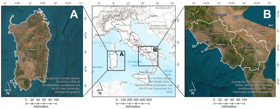
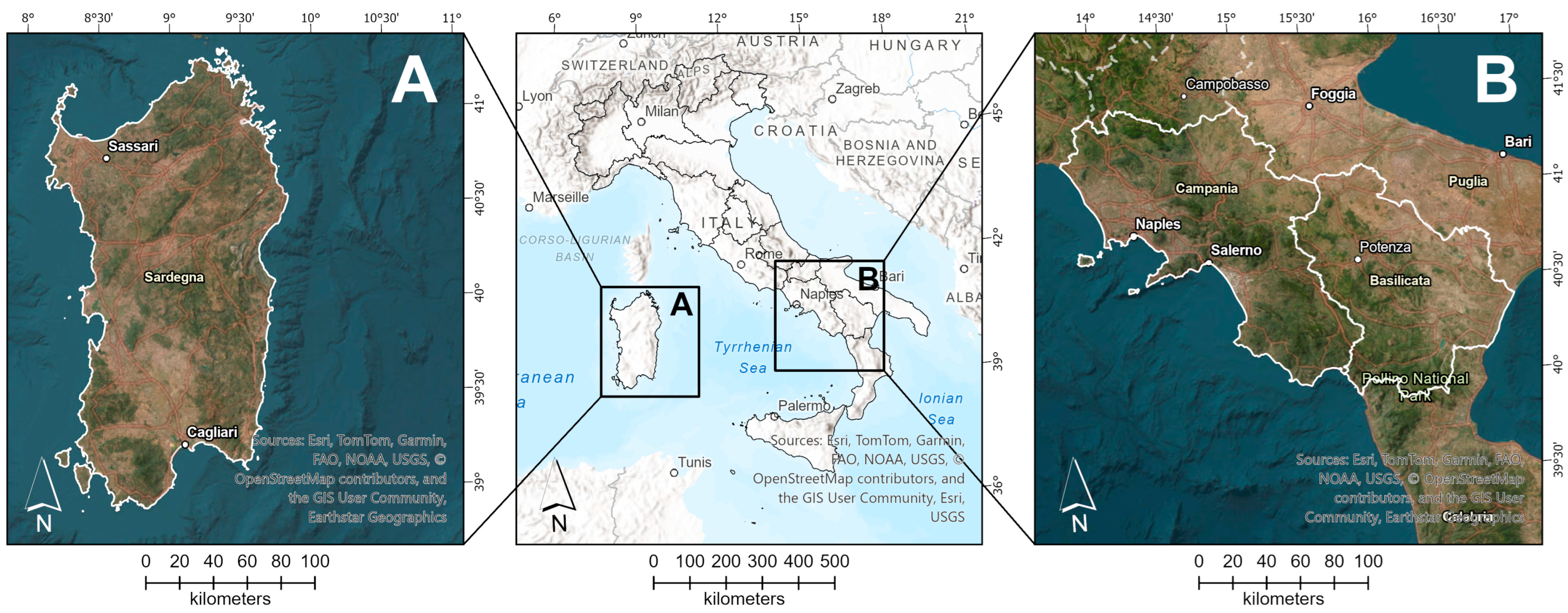
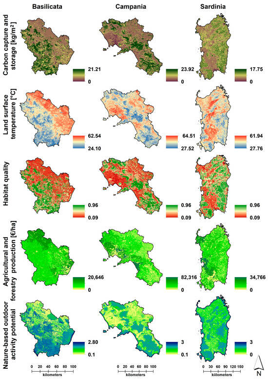
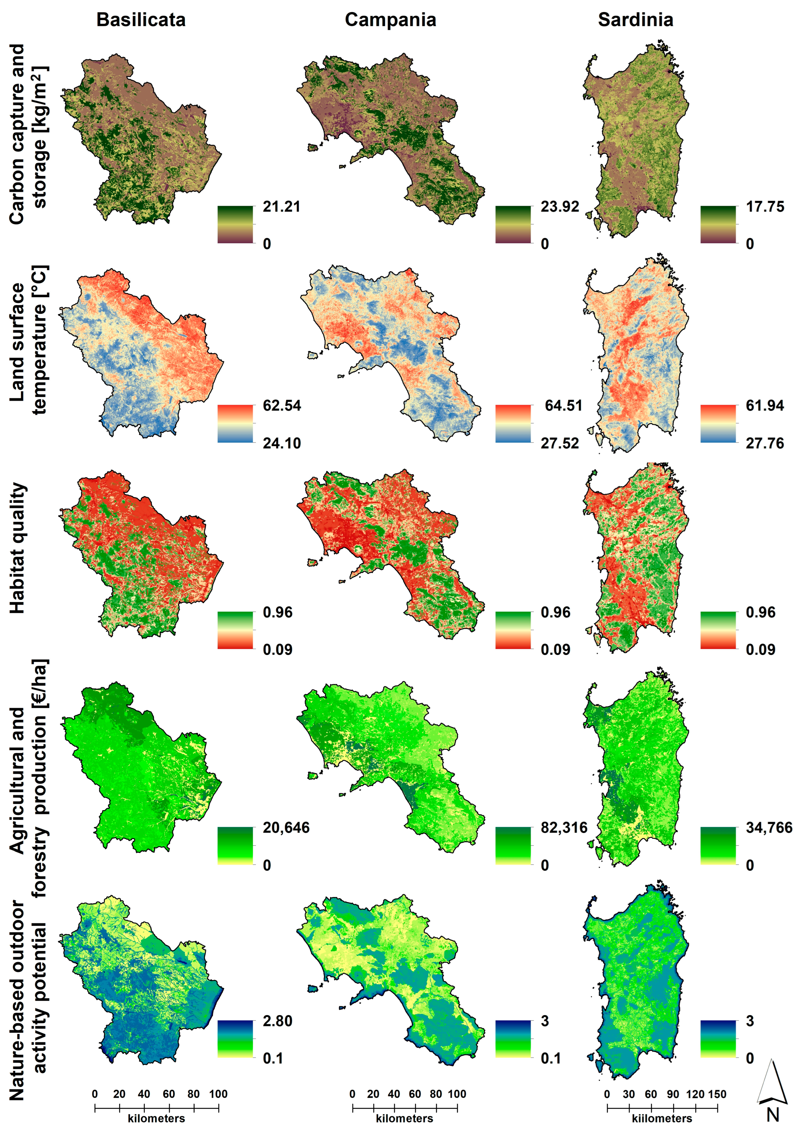
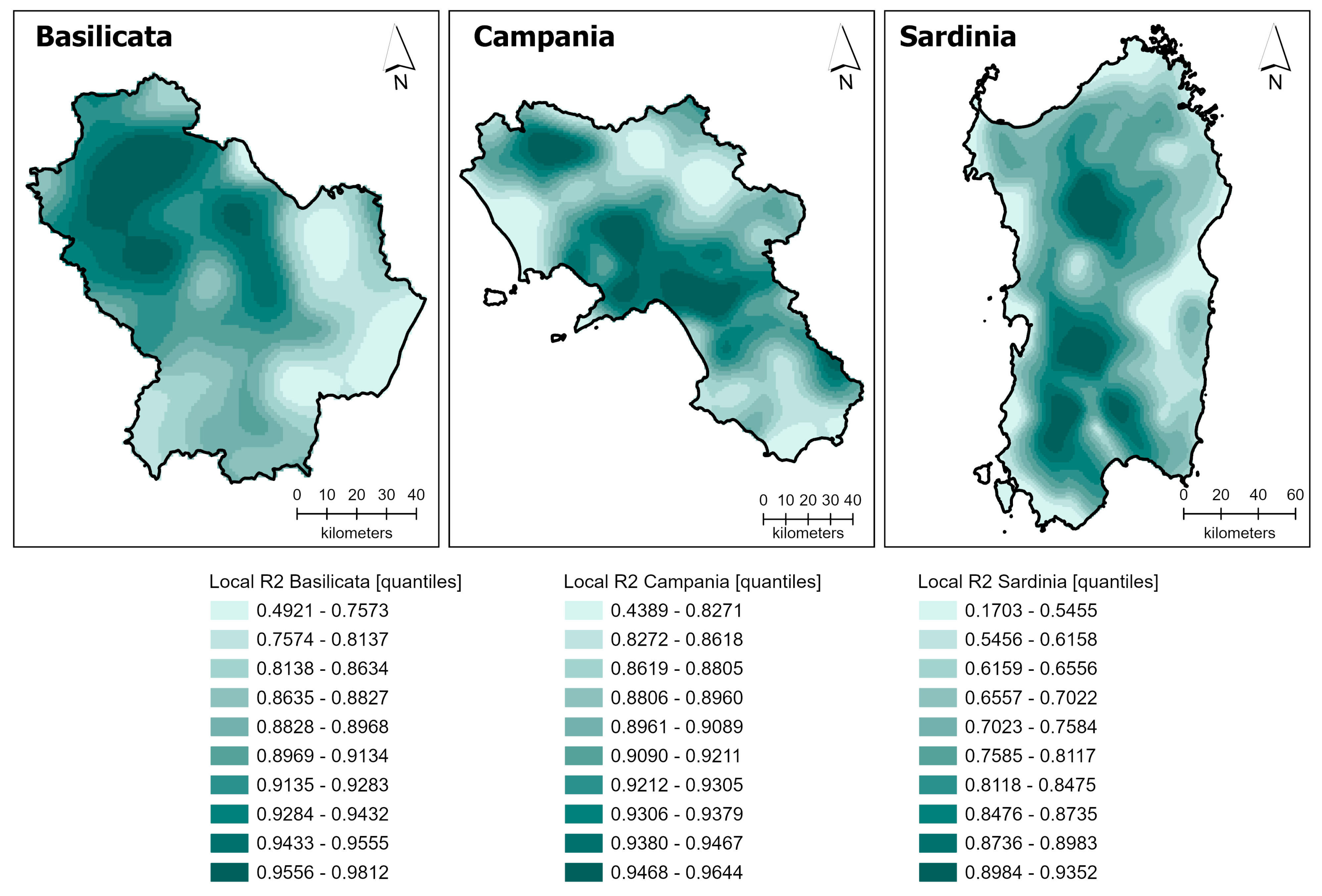
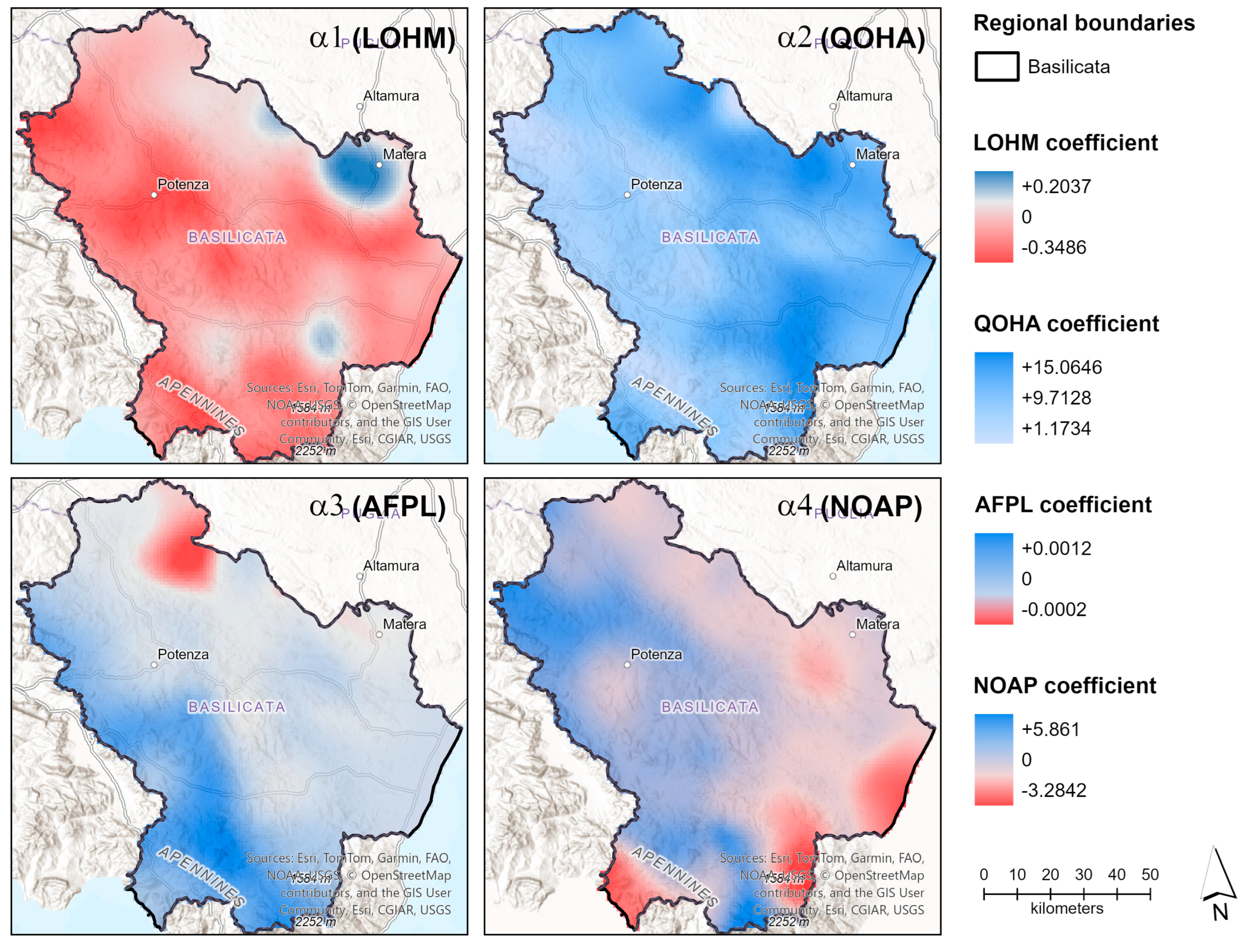
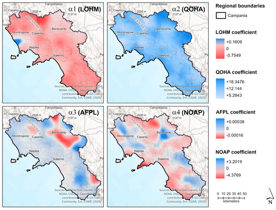
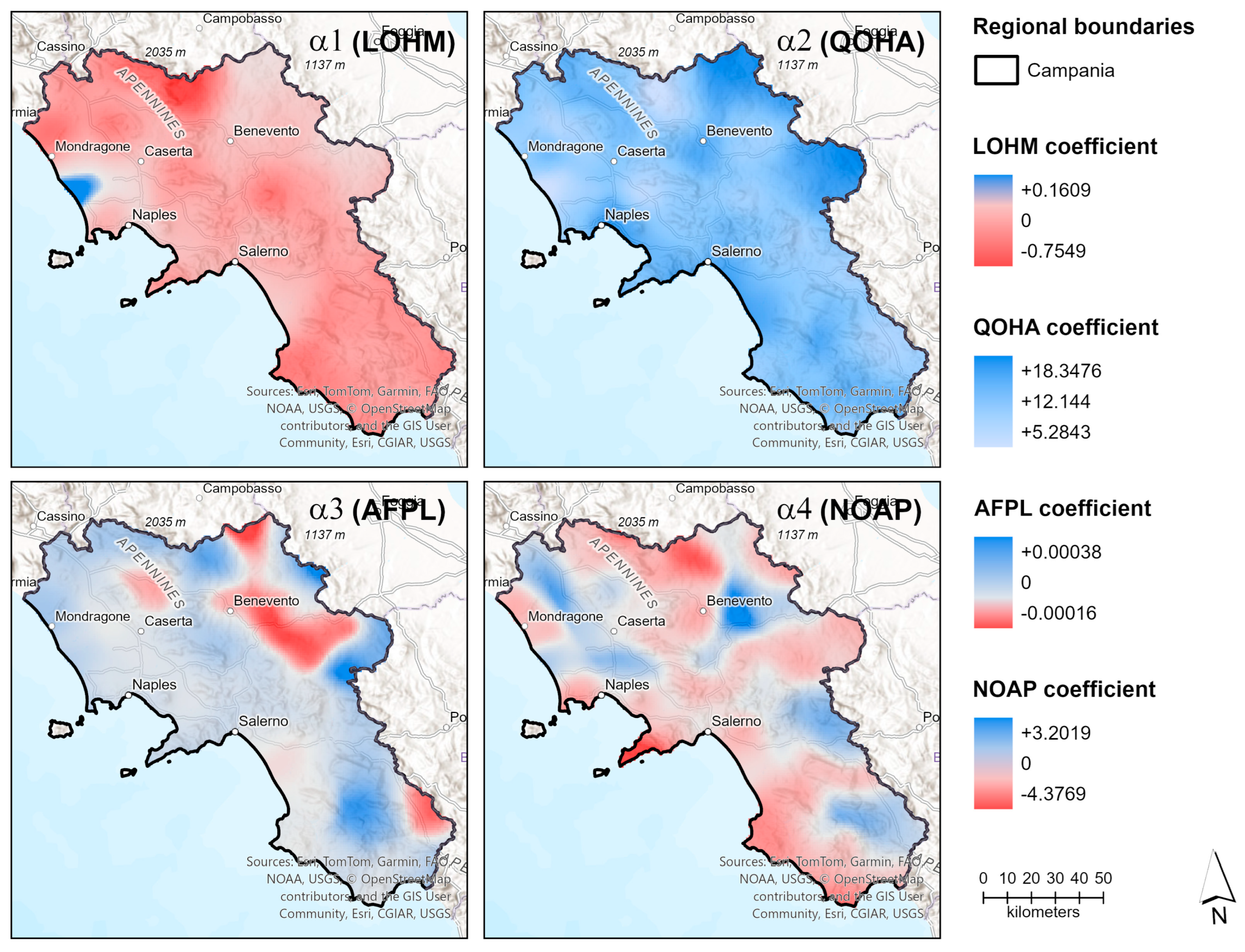
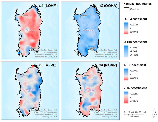
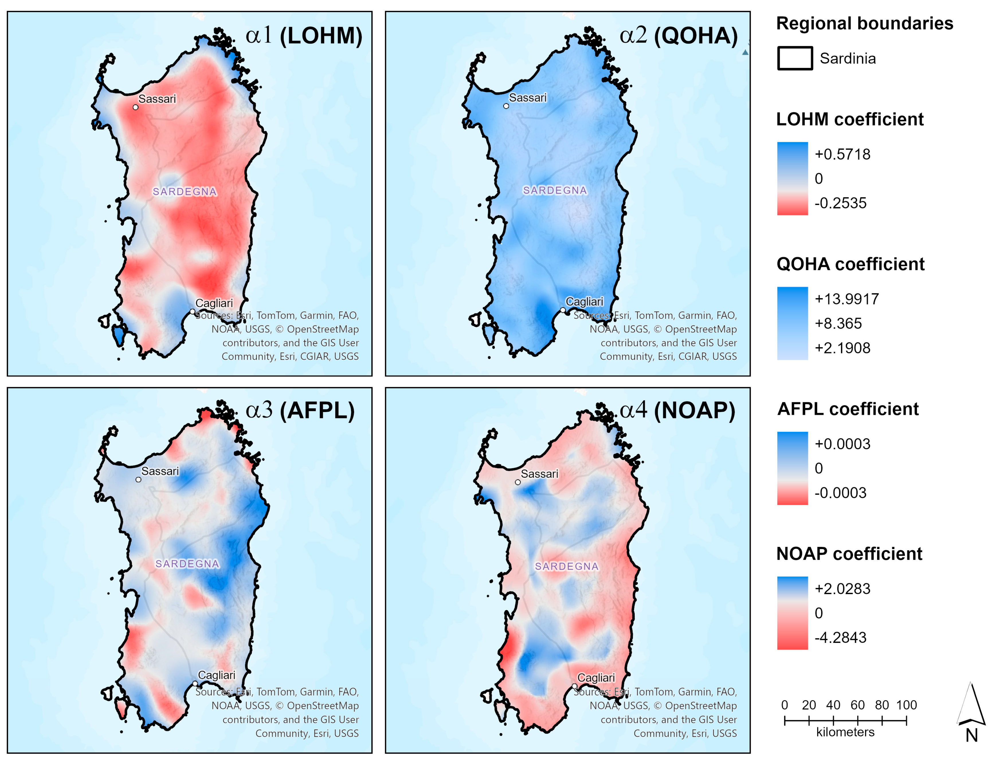

Disclaimer/Publisher’s Note: The statements, opinions and data contained in all publications are solely those of the individual author(s) and contributor(s) and not of MDPI and/or the editor(s). MDPI and/or the editor(s) disclaim responsibility for any injury to people or property resulting from any ideas, methods, instructions or products referred to in the content. |
© 2026 by the authors. Licensee MDPI, Basel, Switzerland. This article is an open access article distributed under the terms and conditions of the Creative Commons Attribution (CC BY) license.