


Abstract
Distributed photovoltaic (PV) systems play an important role in supporting low-carbon and sustainable distribution network development; however, their high-penetration integration can cause nodal overvoltage, as midday PV generation often exceeds local demand and net reverse power flows accumulate along feeders. Existing studies mainly focus on technical mitigation, while entity-level responsibility quantification and its translation into differentiated mitigation tasks remain insufficiently explored. This paper proposes an overvoltage mitigation method integrating Shapley-value-based responsibility quantification with active–passive-responsibility-driven task allocation. Reverse power flow quotas are determined using the Technique for Order Preference by Similarity to Ideal Solution (TOPSIS) by considering the differentiated impacts of PV entities on power flow distribution and nodal voltage response. The load-weighted voltage deviation index is adopted as the coalition cost function, and the Shapley value is used to quantify each entity’s overvoltage responsibility share. Active and passive responsibilities are characterized through the net reverse power ratio and reactive power–voltage sensitivity, respectively, establishing a mapping mechanism from responsibility shares to active power curtailment and reactive power regulation tasks. A multi-objective optimization model that jointly considers line losses, PV curtailment, fairness deviation, and task-allocation deviation is constructed and solved using the whale optimization algorithm. Case studies on the IEEE 33-bus system show that the proposed method reduces the maximum network voltage from 1.25 pu to 1.052 pu and eliminates all overvoltage violations. Compared with a cluster-based scheme, the 24-h cumulative line loss is reduced by 30.6%, and the fairness deviation is significantly lowered, thereby supporting the sustainable, economical, and equitable operation of distribution networks with high distributed PV penetration.
1. Introduction
With the continued advancement of carbon peaking and carbon neutrality goals and the rapid development of distributed PV, the penetration of distributed PV in distribution networks has increased steadily. When the ratio of total distributed PV generation capacity to the local load demand becomes sufficiently large, the distribution network is regarded as having high PV penetration. Under such conditions, distribution networks involve numerous connected entities with diverse capacities and complex network coupling relationships. Under the operating mode of “self-consumption with surplus fed to the grid,” midday periods often exhibit high PV output while local load demand remains low. As a result, the net reverse power flows of multiple entities accumulate along feeders, causing power to flow back to the upstream grid and thereby leading to nodal voltage rise and even voltage violations. The overvoltage problem not only constrains the further improvement of distributed PV hosting capacity, but also directly affects the safe and stable operation of distribution networks, making it a critical issue under high distributed PV penetration [1,2,3]. Therefore, PV-induced overvoltage mitigation is not only a technical requirement for voltage security, but also a sustainability-related requirement for accommodating more local renewable generation and supporting reliable low-carbon distribution network operation.
Existing studies on PV-induced overvoltage have mainly focused on technical mitigation. In terms of reactive power regulation, References [4,5] proposed overvoltage mitigation methods based on local reactive power support and inverter reactive power control, while Reference [6] further investigated the coordinated control of on-load tap changers and smart inverters to enhance voltage regulation capability in unbalanced distribution networks. In terms of active power regulation and multi-resource coordination, Reference [7] proposed a feeder voltage regulation method based on coordinated control of distributed energy storage, Reference [8] applied distributed battery energy storage to voltage support in distribution networks with high PV penetration, and Reference [9] mitigated voltage violations through coordinated control of electric vehicle batteries and PV active power curtailment. In terms of demand–side participation, Reference [10] proposed a coordinated voltage control method incorporating residential demand response under multiple uncertainties, and Reference [11] comparatively evaluated various overvoltage mitigation techniques for low-voltage distribution networks. Overall, existing technical mitigation studies have expanded from single reactive power control to active power regulation and multi-resource coordinated control. However, their fairness mechanisms are typically defined from the perspective of control burden, participation balance, operational boundary, network partitioning, or allocation proportionality, without explicitly quantifying each entity’s marginal contribution; therefore, the resulting allocation may appear balanced yet remain inconsistent with actual responsibility. In contrast, Shapley-value-based responsibility quantification evaluates the average marginal effect of each entity across possible coalitions, thereby providing a game-theoretically fair basis for differentiated mitigation task allocation.
As the scale of PV integration continues to grow, mitigation methods centered on a single device or entity can no longer simultaneously ensure mitigation effectiveness, operational economy, and fairness. Research has therefore shifted toward coordinated optimization at the system level. Reference [12] constructed a multi-timescale coordinated voltage/reactive power control framework, Reference [13] proposed a three-stage robust inverter control method for high-PV-penetration scenarios, and Reference [14] studied voltage/reactive power coordination from the perspective of rolling-horizon multi-objective robust optimization. In terms of operational boundaries and fair coordination, Reference [15] defined export limits for PV-rich low-voltage networks, while Reference [16] incorporated fairness into Volt/Var control and PV curtailment coordination. Reference [17] proposed a hierarchical decentralized voltage control method based on network partitioning, Reference [18] introduced a two-level overvoltage control strategy, and References [19,20] further considered demand–resource participation and fair payoff allocation. However, mitigation-task allocation among multiple entities still largely relies on topological partitioning or uniform rules, which do not clarify each entity’s actual contribution to overvoltage formation and therefore provide an insufficient fairness basis, and some entities may bear mitigation burdens that do not match their actual contributions.
In practice, overvoltage in distribution networks arises from the combined effect of net reverse power flows from multiple distributed PV entities. These entities compete for the limited reverse power accommodation capability of the network and can therefore be modeled as participants in a cooperative game. Cooperative game theory provides an effective tool for responsibility attribution and fair allocation in such multi-entity coupled scenarios. The Shapley value satisfies additivity, efficiency, and fairness, and has been applied to transmission cost allocation [21], distribution network loss allocation [22,23], and benefit allocation in the aggregated operation of distributed energy resources [24,25]. Reference [26] introduced the Shapley value method to quantify overvoltage responsibility in distribution networks with high distributed PV penetration, representing an important initial exploration of responsibility attribution for PV-induced overvoltage. However, it provides only an ex-post attribution framework that quantifies each entity’s responsibility share but does not establish a mechanism for translating these shares into executable mitigation tasks. Responsibility shares indicate only the relative contribution to overvoltage formation, while practical mitigation further depends on each entity’s reverse-power ratio, voltage sensitivity, inverter capability, and operating condition. To address this gap, this paper proposes an active–passive responsibility mapping mechanism that bridges Shapley-value-based responsibility quantification and coordinated mitigation task allocation.
Accordingly, this paper proposes an overvoltage mitigation method for distribution networks with high distributed PV penetration based on Shapley-value-based responsibility quantification and active–passive-responsibility-driven task allocation. The main contributions of this paper are as follows:
- (1)
- An overvoltage responsibility quantification method for distribution networks with high distributed PV penetration is proposed. By integrating power flow impact and voltage response differences, the method constructs a baseline reverse power flow quota for each entity and employs the Shapley value method to calculate the overvoltage responsibility share of each entity.
- (2)
- An active–passive-responsibility-driven mitigation task mapping method is proposed. By characterizing active responsibility, passive responsibility, and mitigation contribution, the method enables coordinated allocation of active power curtailment and reactive power regulation tasks.
- (3)
- A responsibility-driven optimization model that balances fairness and economy is constructed. By jointly considering line losses, PV curtailment, fairness deviation, and task-allocation deviation, the model achieves optimized allocation of overvoltage mitigation tasks in distribution networks.
2. Overvoltage Responsibility Quantification Based on the Shapley Value
2.1. Reverse Power Flow Quota Determination Based on Power Flow Impact and Voltage Response
After the integration of high-penetration distributed PV, different entities exhibit markedly different impacts on the distribution network depending on their output scale, access location, line path, and nodal voltage response characteristics. Allocating reverse power flow reference values solely by installed capacity or in an equal-share manner cannot accurately reflect these differences. Therefore, entity-level differences are characterized in terms of power flow impact and voltage response, and the reverse power flow quota is determined accordingly.
2.1.1. Power Flow Impact Characterization Based on the DistFlow Model
For radial distribution networks, the impact of net reverse power flows from distributed PV entities on branch power flows is primarily propagated upstream along the common path from the access point to the slack bus. The LinDistFlow model can represent this propagation and facilitates the construction of entity-level branch impact vectors; it is therefore adopted here.
For PV entity i located at node , when its active power injection increases by , the power flow change on branch l can be expressed as follows:
where denotes the set of branches on the path from the slack bus to the access node . The impact factor of entity i on branch l is further defined as follows:
The branch impact vector of entity i is composed of the impact factors for all branches:
where L is the total number of branches in the system.
Equations (1)–(3) indicate that the impact of entity power injection is primarily distributed along the common path from the entity to the slack bus. An access point closer to the feeder end generally leads to more affected branches and a more pronounced impact on the overall network power flow distribution. The branch impact vector can thus characterize the degree of influence of an entity on the power flow structure of the distribution network.
It is noted that the proposed branch-impact vector is derived under the radial feeder assumption. For weakly meshed or flexibly interconnected distribution networks, the unique upstream path no longer exists, and the proposed path-based formulation would need to be extended using a generalized branch-flow sensitivity matrix, such as a PTDF-based or Jacobian-based approach. The present study focuses on radial feeders, which remain the dominant topology in medium- and low-voltage distribution systems.
2.1.2. Voltage Impact Characterization Based on the Voltage Sensitivity Matrix
Since overvoltage ultimately manifests as nodal voltage violations, power flow analysis alone is insufficient; the effect of entity power injection on nodal voltages must also be examined. To this end, the active power–voltage sensitivity matrix is constructed in the vicinity of the AC power flow operating point, and the voltage impact vector of each entity on all network nodes is defined:
where is the active power–voltage sensitivity matrix; is the nodal voltage magnitude vector; is the rated voltage; and P is the nodal active power injection vector.
For PV entity i located at node , the voltage impact vector of its active power injection perturbation on all network nodes is defined as follows:
where is the -th standard basis vector.
Equations (4) and (5) indicate that different entities have notably different impacts on nodal voltages. In general, entities located at feeder ends, along lines with higher impedance, or near weak nodes exhibit higher sensitivity values and a more pronounced effect on local voltage rise.
2.1.3. Reverse Power Flow Quota Determination Based on Comprehensive Evaluation Weights
Each entity’s contribution to overvoltage is jointly characterized by its power-flow impact on feeder branches and its voltage impact at network nodes, which respectively reflect the branch-level and nodal-level mechanisms of overvoltage formation. The TOPSIS method is therefore applied to combine these two indicators into a composite evaluation for quota allocation. After obtaining the power-flow impact and voltage-impact information, the TOPSIS method is used to evaluate the comprehensive impact degree of each PV entity. To remove dimensional and scale inconsistencies, the original impact matrices are normalized. The TOPSIS calculation process is as follows:
- (1)
- Matrix normalization. Taking the power-flow impact matrix as an example:
- (2)
- Determination of positive and negative ideal solutions and :
For the power-flow impact matrix, ; for the voltage-impact matrix, .
- (3)
- Calculate the distances between entity and the positive and negative ideal solutions:
- (4)
- Calculate the overall power-flow impact score of the K PV entities:
Similarly, the overall voltage-impact score of the K PV entities can be obtained in the same manner.
Since the power-flow impact and voltage impact are both important for reverse power flow quota allocation and no priority is imposed between them, the two closeness degrees are averaged as follows:
Using as the proportional coefficient, the quota of each entity is allocated proportionally under the constraint of the total net reverse power capacity that the system can accommodate:
where is the total net reverse power capacity corresponding to the critical voltage violation boundary of the system, and is the total number of distributed PV entities. In practice, is obtained by a bisection-based injection search, where TOPSIS-ratio-based trial injections are verified by AC power flow until the maximum-voltage mismatch satisfies the prescribed tolerance. This value serves solely as the proportional basis for obtaining the baseline quota of each entity.
Based on the obtained baseline quota, entities whose actual reverse power flow exceeds their quota are regarded as having encroached on the voltage safety margin and are therefore included in the subsequent responsibility quantification. The final responsibility of each entity must be further determined according to the actual violation conditions. To justify the use of TOPSIS for quota allocation, a comparison with entropy-weighting, equal-allocation, and capacity-based quota methods is provided in Appendix A. The results show that TOPSIS provides a balanced performance among mitigation effort, voltage security, loss, and fairness.
2.2. Overvoltage Responsibility Allocation Based on Coalition Marginal Contributions
The reverse power flow quota identifies whether each entity has crossed the voltage safety boundary, but it does not determine the responsibility share each entity should bear. Overvoltage results from the combined action of multiple entities, which differ in their network coupling effects and marginal impacts on voltage. Therefore, responsibility should be quantified based on each entity’s marginal contribution to overvoltage severity, rather than assigned in proportion to the excess ratio.
2.2.1. Coalition Cost Construction Based on the Load-Weighted Voltage Deviation Index
Before computing the Shapley value, the coalition cost function must first be determined. Existing overvoltage evaluation indices mainly include the maximal voltage deviation index (MVDI) [27], the average voltage deviation index (AVDI) [28], and the load-weighted voltage deviation index (LVDI) [29]. Among these, MVDI primarily reflects the voltage deviation at the most severely violated node, AVDI reflects the overall voltage deviation level across all violated nodes, and LVDI further incorporates nodal load weights on this basis. Therefore, consistent with Reference [26], this paper adopts LVDI as the coalition cost function, as it considers both voltage violation severity and load-weighted nodal importance:
where is the load-weighted voltage deviation index at time t; is the set of nodes experiencing overvoltage in the distribution transformer area at time t; is the upper voltage limit of the distribution network; represents the load proportion weight of node i within the set of violated nodes , defined as , where is the active load at node i at time t. When , .
2.2.2. Entity Overvoltage Responsibility Calculation Based on the Shapley Value
After the coalition cost function is determined, the Shapley value is used to compute the average marginal contribution of each entity to the coalition cost, which is further normalized to obtain the overvoltage responsibility share of each entity:
where is the Shapley value of distributed PV entity i at time t, representing its overvoltage responsibility; denotes any coalition containing entity i; is the set of all distributed PV entities whose actual reverse power flow exceeds their quota at time t; is the overvoltage index when all entities in coalition have reverse power flows exceeding their quotas; is the overvoltage index after removing entity i from coalition (i.e., entity i operates at its quota level); and are the cardinalities of sets and , respectively; and is the normalized overvoltage responsibility share of entity i at time t. The set includes only entities whose actual net reverse power flow exceeds their quota. Entities that do not exceed their quotas are regarded as operating within the pre-defined voltage safety margin and are therefore not assigned additional excess responsibility. This does not imply that their injections have no physical voltage impact, but rather that such impact is considered acceptable under the quota-based baseline.
Equations (14) and (15) show that the responsibility share reflects each entity’s average driving effect on overvoltage risk across all possible coalitions. This formulation captures both network coupling and entity-level heterogeneity in the overvoltage formation process. Compared with capacity-based or excess-ratio-based allocation, this approach more faithfully captures each entity’s actual contribution to overvoltage. However, responsibility shares quantify each entity’s contribution to overvoltage rather than prescribe control quantities; their translation into mitigation tasks requires further modeling, as developed in Section 3.
3. Active–Passive Responsibility-Driven Overvoltage Mitigation Method for Transformer Areas
The responsibility shares obtained in Section 2 quantify each entity’s contribution to overvoltage formation, but they cannot be directly translated into mitigation quantities. In practice, overvoltage mitigation relies on both active power curtailment and reactive power regulation, and entities differ in their suitability for these two actions. This section therefore distinguishes active and passive responsibilities and establishes a mapping from responsibility shares to coordinated mitigation tasks.
3.1. Active and Passive Responsibility Characterization
3.1.1. Active Responsibility Characterization Based on Net Reverse Power Ratio
Under the “self-consumption with surplus fed to the grid” operating mode, the higher the proportion of an entity’s net reverse power flow relative to its PV output, the stronger its direct contribution to overvoltage formation. Accordingly, the ratio of reverse power flow to PV output is defined as the active responsibility indicator:
where is the net reverse power flow of entity i at time t; is the PV output of entity i at time t; is the local load of entity i at time t; and is the normalized active responsibility indicator of entity i at time t.
When , . Entities with higher active responsibility should therefore be prioritized for active power curtailment. Under low-light or heavy-load conditions, , and the net reverse power is set to zero according to Equation (16); in this case, active responsibility associated with net reverse power injection is not assigned. In this study, the net reverse power is calculated from entity-level PV output and local load, as shown in Equation (16). In practice, can be obtained from inverter monitoring, and can be obtained from user-side metering.
3.1.2. Passive Responsibility Characterization Based on Reactive Power–Voltage Sensitivity
Unlike active responsibility, passive responsibility reflects the voltage regulation capability at each entity’s location; in a radial network, identical reactive power injections at different nodes produce varying voltage reduction effects on the violated region. To capture this difference, a passive responsibility indicator is constructed based on the reactive power–voltage sensitivity matrix:
where is the reactive power–voltage sensitivity matrix at the operating point at time t; is the nodal reactive power injection vector; represents the voltage change at violated node k when entity i injects unit reactive power at its access node ; is the node weight normalized by the violation magnitude, defined as ; and is the voltage violation magnitude at node k at time t.
The active and passive responsibilities described above belong to the responsibility characterization layer and cannot be directly mapped to control quantities in a proportional manner. A mitigation contribution layer is therefore introduced to bridge this characterization layer and control decision-making.
3.2. Mapping Mechanism from Responsibility to Mitigation Tasks
Overvoltage mitigation in distribution networks depends not only on the magnitude of entity responsibility but also on the violation magnitude at violated nodes, the voltage-regulation capability of each entity, and the adjustable range of equipment. Therefore, the relationship between responsibility shares and mitigation contributions must first be established, after which the task-allocation ratios for active power curtailment and reactive power regulation can be determined based on those mitigation contributions.
3.2.1. Mitigation Contribution Modeling Based on Violation Magnitude
The voltage at node k at time t before mitigation is denoted by , and the violation magnitude is defined as follows:
In the vicinity of the operating point, the active power–voltage reduction coefficient and the reactive power–voltage reduction coefficient of entity i for violated node k are defined as follows:
where and are the corresponding elements in the active power–voltage and reactive power–voltage sensitivity matrices for node k with respect to the access node .
Denoting the active power curtailment of entity i as and its reactive power absorption as , the voltage restoration condition at each violated node requires the following:
The mitigation contribution of entity i is further defined as follows:
Equation (24) represents the local first-order contribution of active power curtailment and reactive power regulation around the operating point. Although the nonlinear coupling between simultaneous P and Q adjustments is not explicitly modeled in this expression, the obtained mitigation results are checked using full AC power flow in the case study.
Equations (20)–(24) show that an entity’s mitigation contribution grows with both the violation magnitude and its voltage reduction capability at the violated nodes.
3.2.2. Mitigation Task Mapping Based on Active–Passive Responsibility Division
With the mitigation contribution model established, the active and passive responsibilities are used to determine the task-allocation ratios between active power curtailment and reactive power regulation, which are defined as follows:
where and denote the expected active and reactive task-allocation ratios of entity i at time t, respectively. Equations (25) and (26) map active and passive responsibilities to the expected active and reactive task proportions.
3.3. Responsibility-Driven Multi-Objective Optimization Model and Solution
Based on the mitigation contribution and control task allocation established in Section 3.2, a responsibility-driven optimization model is further constructed to coordinate the relationships among voltage safety, operational economy, and responsibility-based fairness.
3.3.1. Responsibility-Driven Multi-Objective Optimization Model
The comprehensive objective function is defined as follows:
To avoid scale effects among different objectives, each sub-objective in Equation (27) is normalized before weighted summation. The weight coefficients are set according to decision-making preferences, with values specified in Section 4. In the equation, , , and represent the weights for the line loss objective, PV curtailment objective, fairness deviation objective, and task division deviation objective, respectively. Each sub-objective is defined as follows:
The line loss objective is as follows:
where is the set of system branches, is the resistance of branch l, and is the current magnitude of branch l at time t.
The PV curtailment objective is as follows:
The fairness deviation objective is as follows:
The task division deviation objective is as follows:
quantifies responsibility-matching fairness, where the mitigation contribution assigned to each entity is expected to be consistent with its Shapley-based overvoltage responsibility share. A smaller indicates that entities with higher overvoltage responsibility undertake proportionally larger mitigation contributions, while entities with lower responsibility avoid disproportionate mitigation burdens. In contrast, measures the deviation of the active–power contribution from the expected active–passive task-allocation ratio, thereby reflecting intra-entity task consistency.
The nodal voltage limits are imposed as hard constraints:
The model must satisfy the inverter capacity constraint:
where is the actual active power output of entity i at time t, and is the rated apparent power capacity of the entity i inverter.
The available reactive power capacity of each entity is constrained by its current active power output:
where is the available reactive power capacity at the current operating point.
Equation (27) enables trade-offs among line losses, PV curtailment, and fairness during the mitigation process. Combined with the nodal violation elimination condition in Equation (23) and the inverter capacity constraint in Equation (33), a complete responsibility-driven optimization model is formed.
3.3.2. Solution Procedure for the Mitigation Model
The established model involves coupled decision-making of both active power curtailment and reactive power regulation, subject to nodal violation elimination conditions and inverter capacity constraints, exhibiting nonlinear and strongly coupled characteristics that are difficult to solve effectively using traditional gradient-based algorithms. The whale optimization algorithm (WOA), which simulates the encircling, spiral-attack, and random-search behaviors of humpback whales, features few parameters and strong adaptability to nonlinear problems, and is therefore adopted to solve the proposed model.
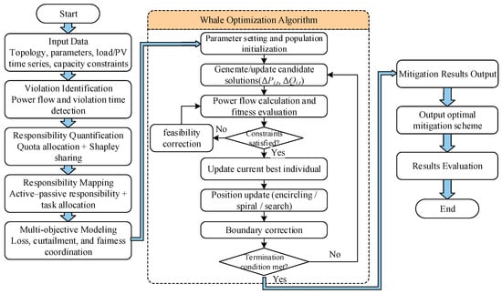
The overall framework is illustrated in Figure 1, and the solution procedure is as follows:
Figure 1.
Overall framework and solution flowchart of responsibility-driven mitigation.
- (1)
- Set the population size, maximum number of iterations, and upper and lower bounds of decision variables, and complete the population initialization.
- (2)
- Generate candidate solutions, perform power flow calculations, and evaluate fitness.
- (3)
- Check whether the constraints are satisfied. If not, apply penalty function processing and feasibility correction. If satisfied, update the current best individual.
- (4)
- Update population positions according to the encircling, spiral, and search mechanisms, and perform boundary correction.
- (5)
- If the termination condition is met, output the optimal allocation results; otherwise, return to step (2) for further iterations.
To further support the selection of WOA, its convergence performance and comparison with PSO and NSGA-II are provided in Appendix B.
4. Case Study Analysis
4.1. Test System and Scenario Setup
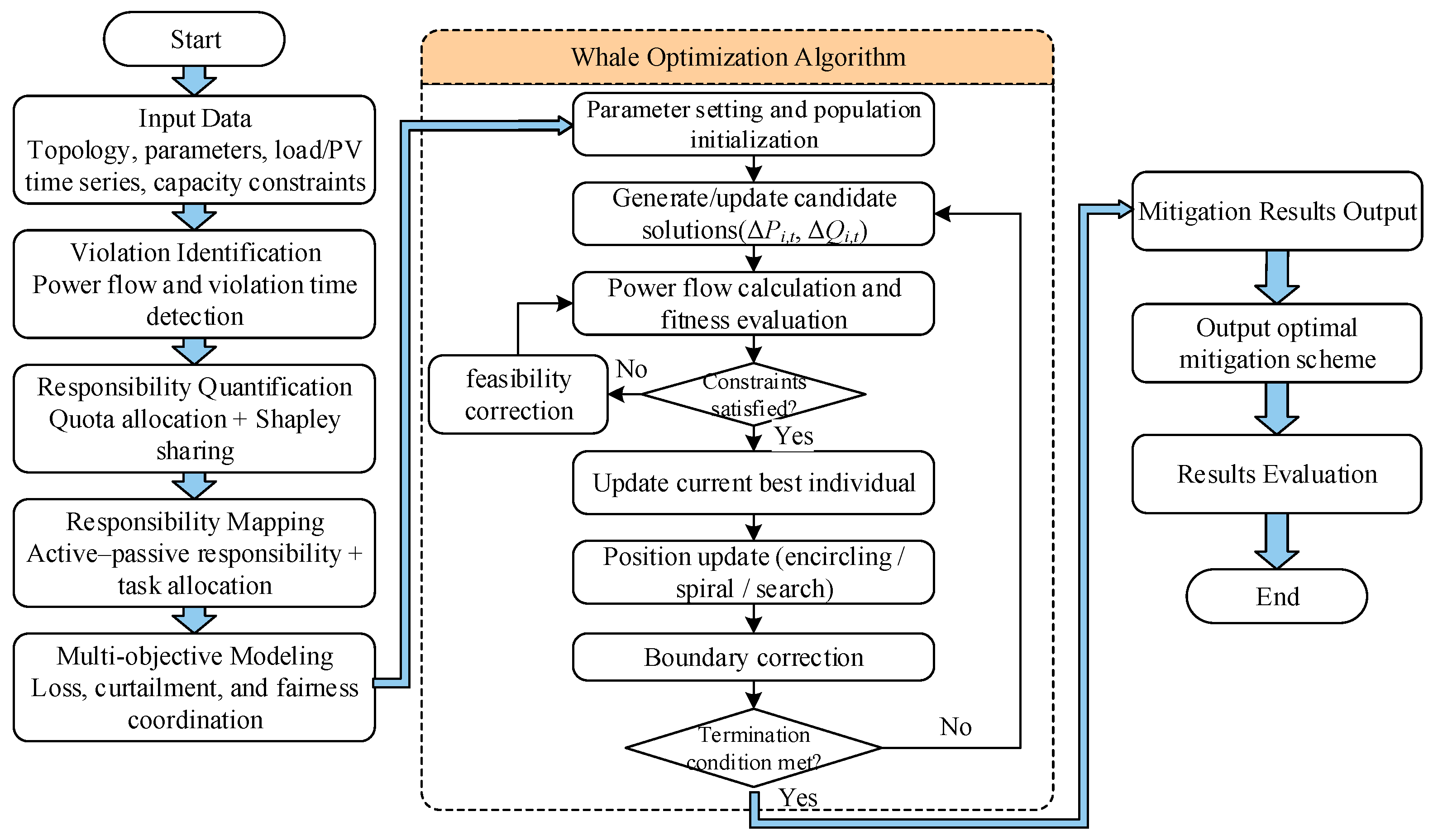
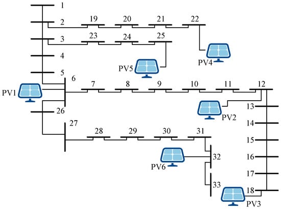
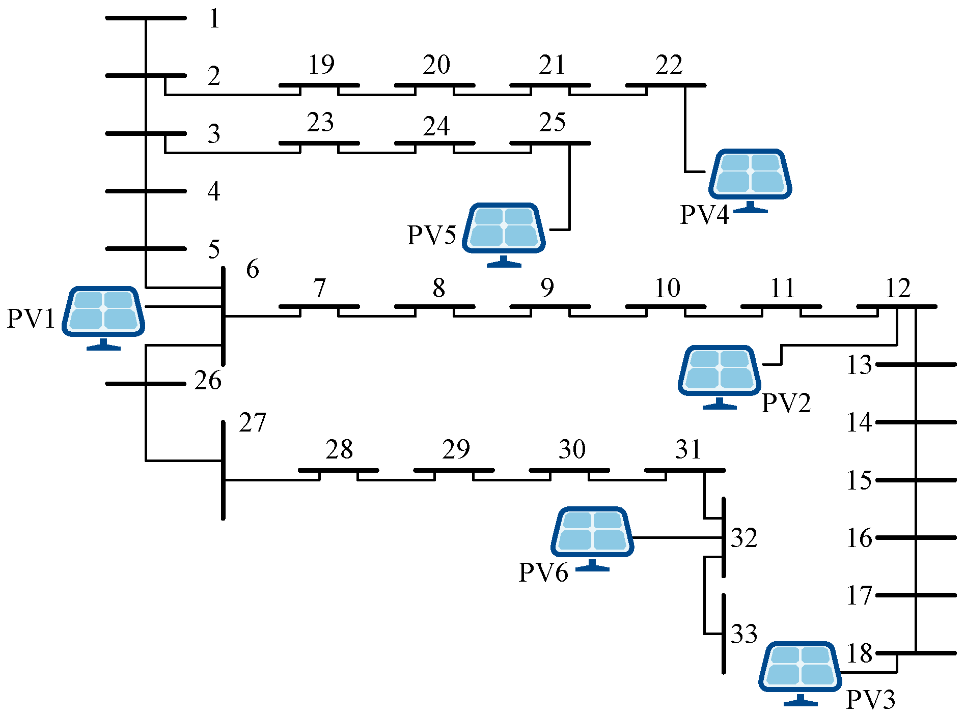
The IEEE 33-bus system is adopted in this paper to validate the proposed method. The total load of the system consists of 1213 residential loads, four commercial/industrial loads, and four public building loads from a certain region in China. The load connected at each node is proportionally allocated based on the initial load data of the IEEE 33-bus system. The time span covers a typical day from 0:00 to 24:00 with a time interval of 15 min. Distributed PV follows the “self-consumption with surplus fed to the grid” principle, with surplus electricity fed into the 10 kV bus through inverters. Six distributed PV entities are configured in the case study, connected at nodes 6, 12, 18, 22, 25, and 32, covering the front, middle, and end sections of the feeders. The system topology and PV connection diagram are shown in Figure 2.
Figure 2.
IEEE 33-bus system topology and PV connections.
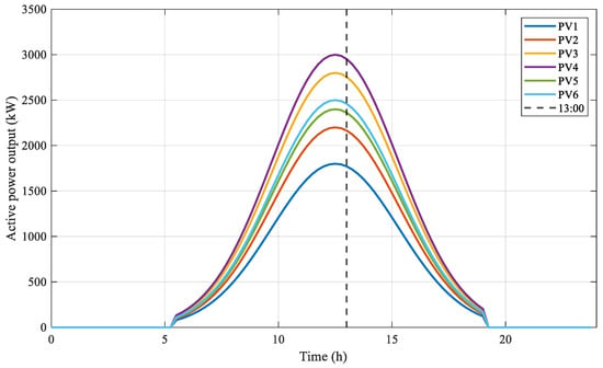
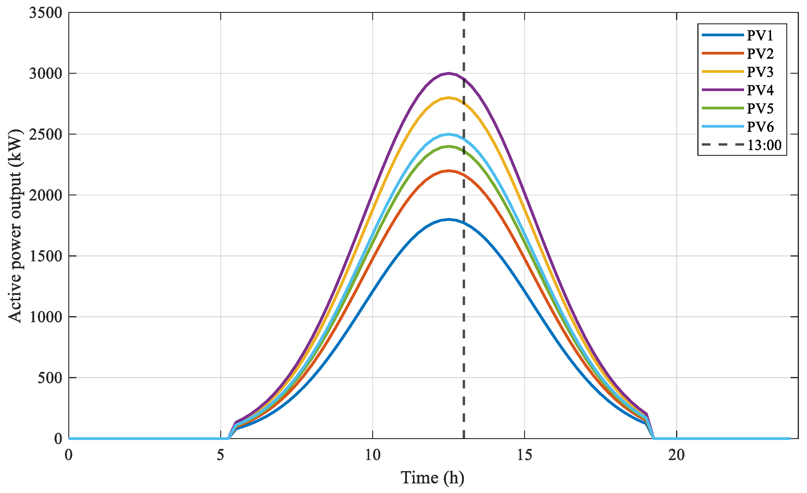
The daily output curves of the distributed PV entities are shown in Figure 3.
Figure 3.
Typical daily active power output curves of distributed PV entities.
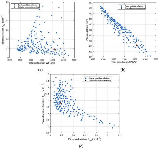
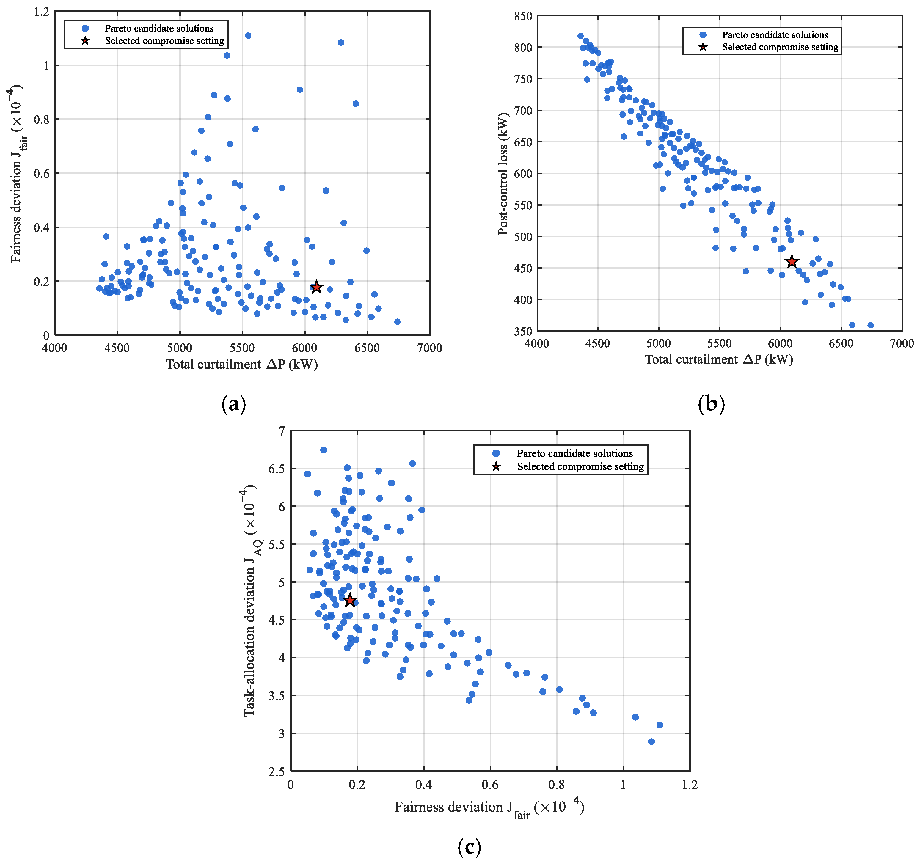
For the comprehensive objective function in Equation (27), the weight coefficients are selected based on a Pareto-based comparison under the above case setting, as shown in Figure 4.
Figure 4.
Pareto candidate solutions under different weight settings. (a) Curtailment versus fairness deviation. (b) Curtailment versus post-control loss. (c) Fairness deviation versus task-allocation deviation.
As shown in Figure 4, the candidate solutions indicate trade-offs among PV curtailment, post-control loss, fairness deviation, and task-allocation deviation. The selected setting is adopted as a feasible compromise rather than a globally optimal point. It gives preference to lower post-control loss and improved fairness while keeping PV curtailment and task-allocation deviation within acceptable ranges. Accordingly, the weights are set as follows: line loss weight λ1 = 0.3, PV curtailment weight λ2 = 0.4, fairness deviation weight λ3 = 0.15, and task-allocation deviation weight λ4 = 0.15.
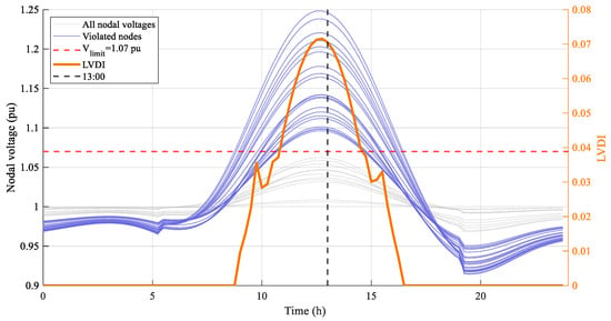
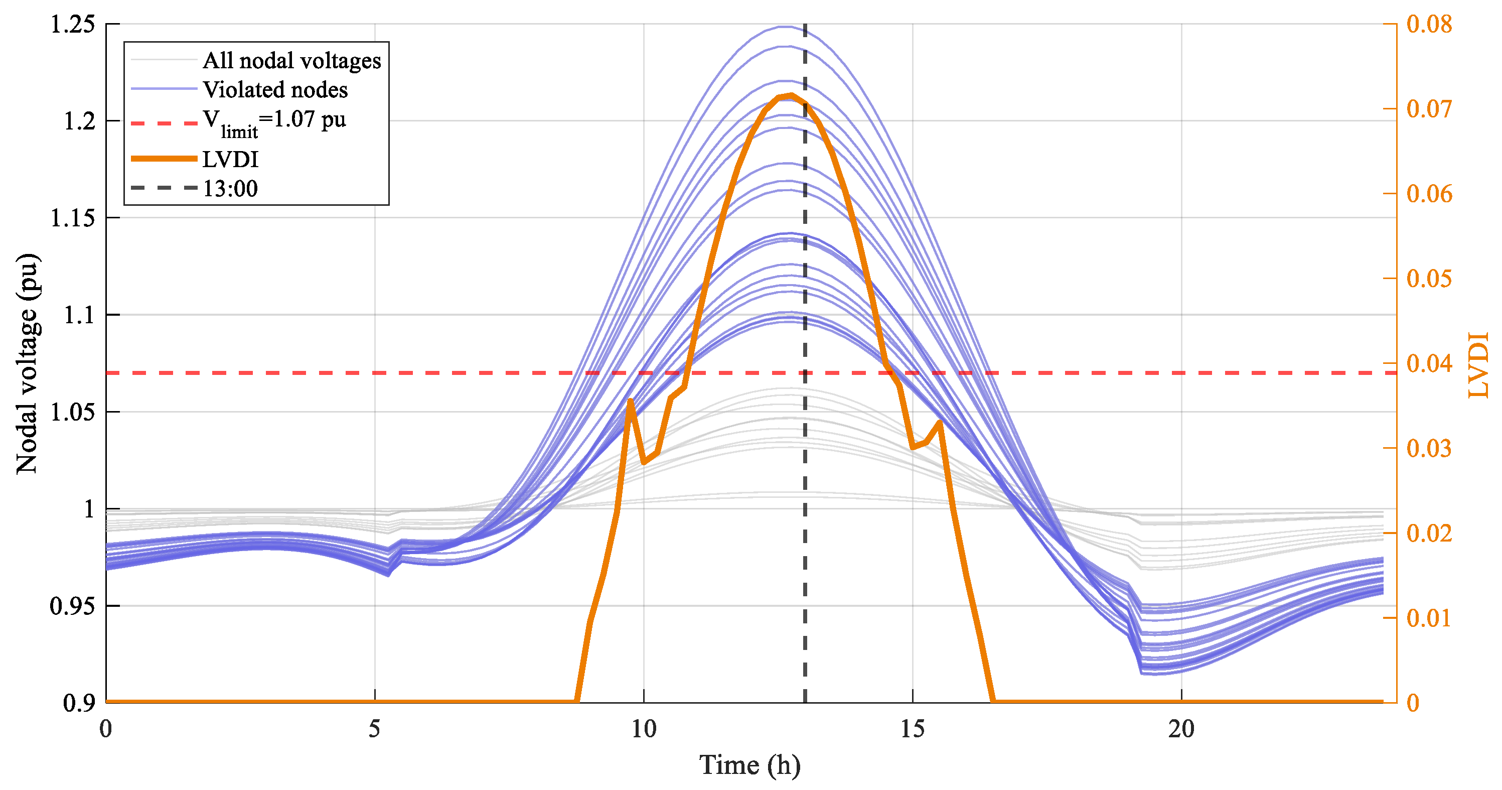
The daily PV output curves and load data are input into the IEEE 33-bus system for power flow calculation. The resulting daily nodal voltage time-series curves and LVDI variation curves are shown in Figure 5.
Figure 5.
Typical daily nodal voltage and LVDI time-series curves (before mitigation).
As shown in Figure 5, nodes 9–18 and 28–33 exhibit significant voltage violations during midday. The LVDI remains nonzero from 8:00 to 16:00 and reaches its peak at 13:00. Therefore, 13:00 is selected as the representative time instant for subsequent responsibility quantification analysis.
4.2. Responsibility Quantification Results Analysis
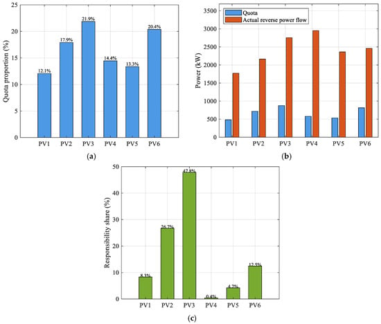
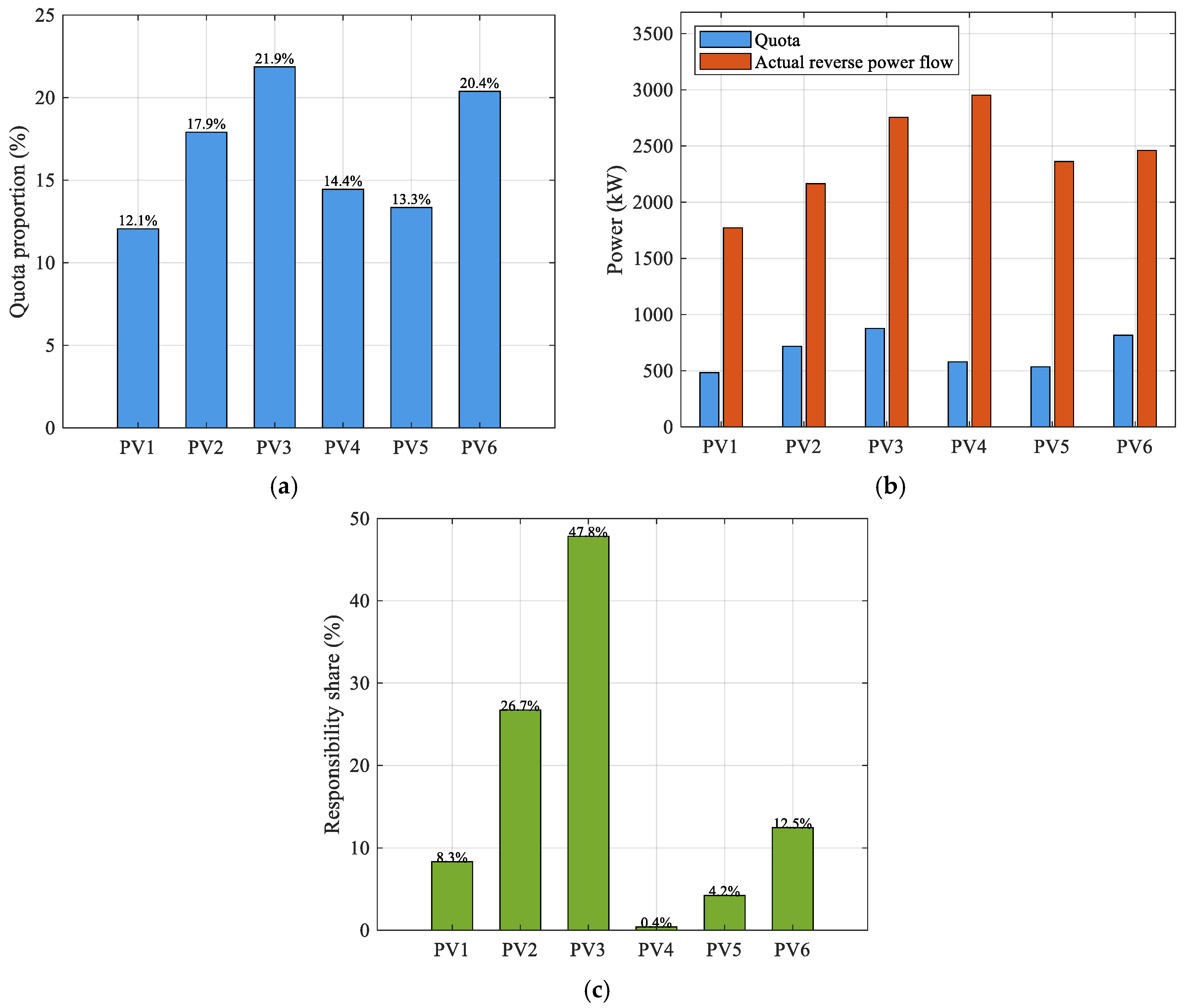
The comprehensive evaluation weights and quota allocation proportions of each entity are calculated using Equations (6)–(12), and the results are shown in Figure 6.
Figure 6.
Responsibility quantification results at 13:00. (a) Quota proportions. (b) Comparison between quota and actual reverse power flow. (c) Responsibility shares.
The quota allocation proportions of each entity are shown in Figure 6a. PV3 and PV6, connected at nodes 18 and 32, respectively, have the highest comprehensive impact on system power flow and voltage, with quota proportions of 21.9% and 20.4%, respectively. PV1, connected at node 6, is located at the front of the feeder and has the lowest comprehensive impact, with a quota proportion of 12.1%. At the representative time instant of 13:00, the actual reverse power flows of all six entities exceed their respective quotas, as shown in Figure 6b, and all are included in the subsequent responsibility quantification.
The overvoltage responsibility quantification results are shown in Figure 6c. Notably, responsibility shares diverge significantly from quota proportions—PV3 holds only a 21.9% quota proportion but bears 47.84% of the responsibility, while PV4 holds 14.4% but only 0.40%—demonstrating that the Shapley value captures marginal contributions across coalitions rather than simply reflecting the absolute magnitude of the quota or reverse power flow. PV2 has the second-highest responsibility share at 26.73%.
The active responsibility , passive responsibility , and expected task-allocation ratios of each entity are calculated using Equations (18) and (19), with detailed results listed in Table 1.
Table 1.
Responsibility quantification and expected task-allocation results at 13:00.
The active responsibilities of all entities exhibit small differences, ranging from 0.933 to 0.990. This is because midday local loads are much lower than PV output for all entities; therefore, the net reverse power ratios are uniformly high. PV5 has a slightly lower active responsibility than the other entities because its local load is relatively larger, resulting in a higher self-consumption ratio and a correspondingly lower net reverse power proportion.
In contrast, the passive responsibility exhibits significant differences closely related to the topological location. PV3, connected at node 18 at the end of the main feeder, is electrically farthest from the slack bus and has the largest accumulated line impedance, resulting in the highest passive responsibility of 1.000. PV2 and PV6, located in the middle section of the main feeder and at the end of a lateral branch, respectively, exhibit intermediate passive responsibilities of 0.666 and 0.417. The remaining entities have limited passive responsibilities: PV1, near the feeder front, has a passive responsibility of 0.289 due to its short electrical distance, whereas PV4 and PV5, located on lateral branches weakly coupled to the main violated region, have passive responsibilities close to zero.
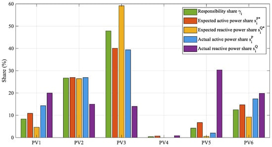
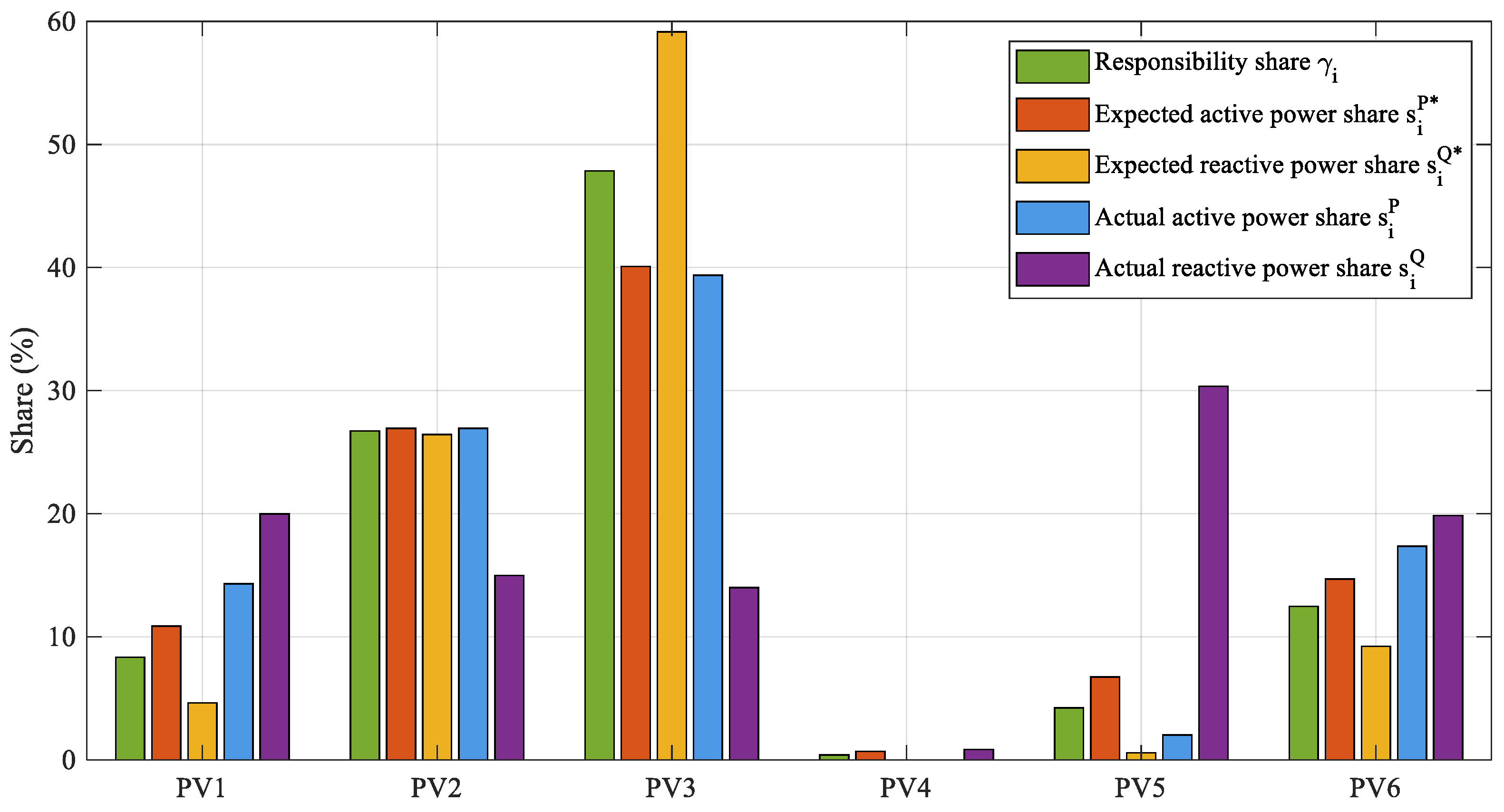
The differences in active and passive responsibilities directly determine the differentiation in expected task allocation: PV3 has approximately equal active and reactive power contribution ratios, PV4 and PV5 almost entirely bear active power curtailment tasks, and PV2 and PV6 undertake both active and reactive power tasks. Figure 7 presents a comparison of responsibility shares, expected task allocation, and actual mitigation shares. The actual mitigation shares are generally consistent with the expected allocation, validating the effectiveness of the active–passive responsibility mapping mechanism.
Figure 7.
Comparison of responsibility shares, expected task allocation, and actual mitigation shares.
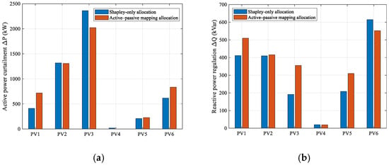
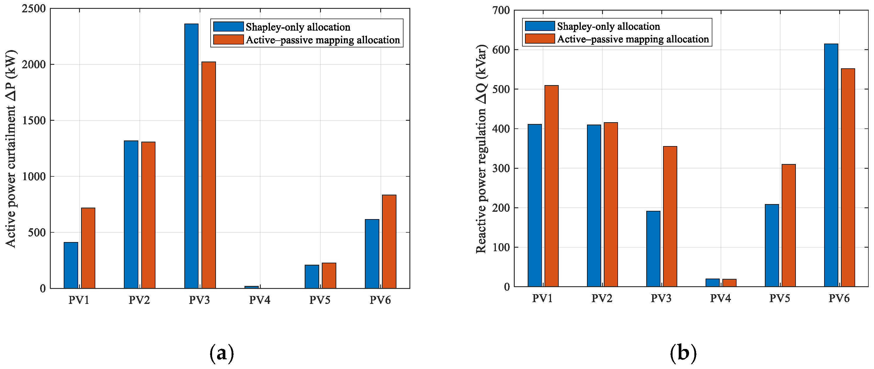
To further clarify the effect of the active–passive responsibility mapping on reactive power regulation, a Shapley-only allocation scheme is compared with the proposed mapping-based scheme, as shown in Figure 8.
Figure 8.
Ablation analysis of active–passive responsibility mapping. (a) Active power curtailment allocation. (b) Reactive power regulation allocation.
As shown in Figure 8, the Shapley-only scheme allocates reactive power regulation mainly according to the overall responsibility shares, resulting in a relatively high regulation task for PV6 and limited regulation for PV3 and PV5. In contrast, the proposed scheme further considers the reactive power–voltage sensitivity of each entity, increasing the regulation tasks of PV3 and PV5 while reducing that of PV6. This indicates that the proposed mapping does not simply follow the Shapley responsibility share, but redistributes reactive power regulation according to passive responsibility and voltage regulation capability.
4.3. Mitigation Effectiveness and Scheme Comparison
4.3.1. Responsibility-Driven Mitigation Effectiveness
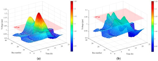
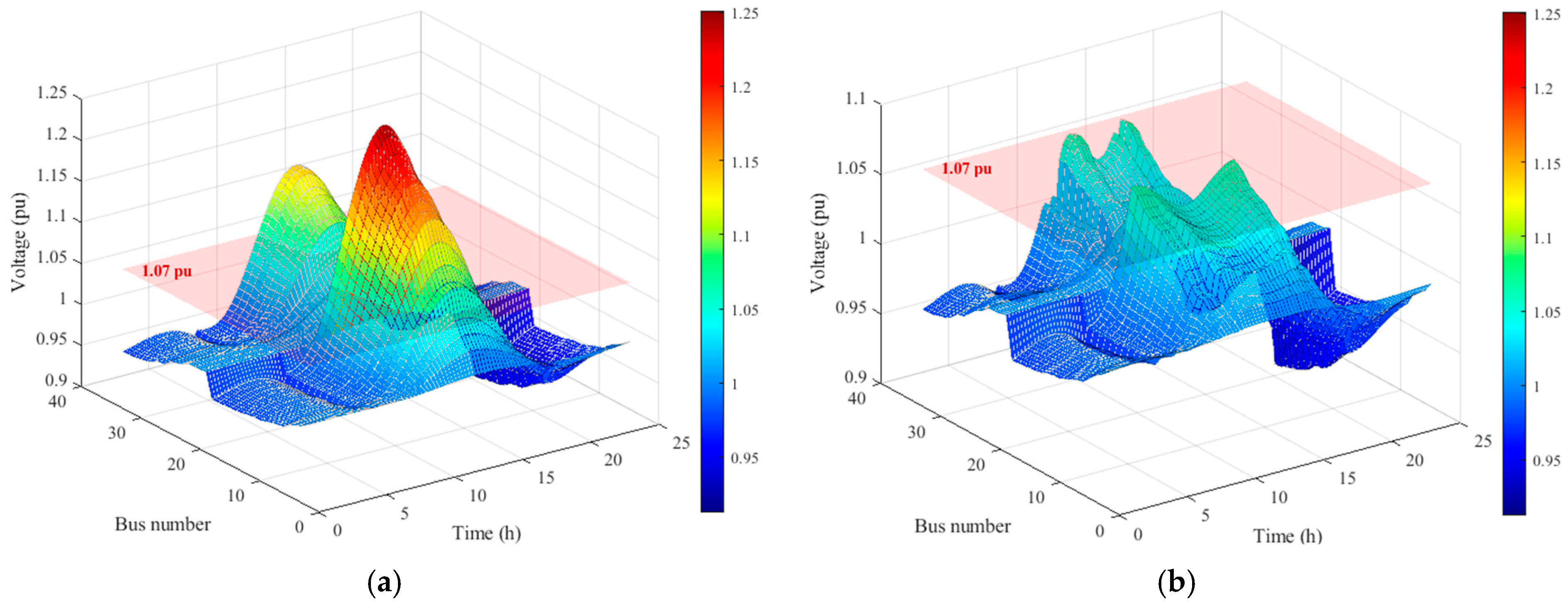
Based on the responsibility quantification results and the active–passive responsibility mapping, the mitigation tasks of each entity are obtained by solving the proposed optimization model using the whale optimization algorithm. The 24-h spatiotemporal distributions of network-wide nodal voltages before and after mitigation are shown in Figure 9. Before mitigation, a large-scale voltage bulge appears during midday, reaching a maximum of 1.25 pu, with a large area exceeding the violation threshold. After mitigation, the voltage surface falls entirely below the violation threshold, with the maximum network voltage reduced to 1.052 pu, confirming that the proposed method effectively eliminates all overvoltage violations.
Figure 9.
The 24-h spatiotemporal distribution of nodal voltages before and after mitigation. (a) Before mitigation. (b) After mitigation.
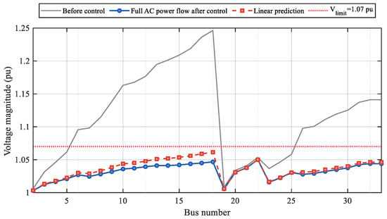
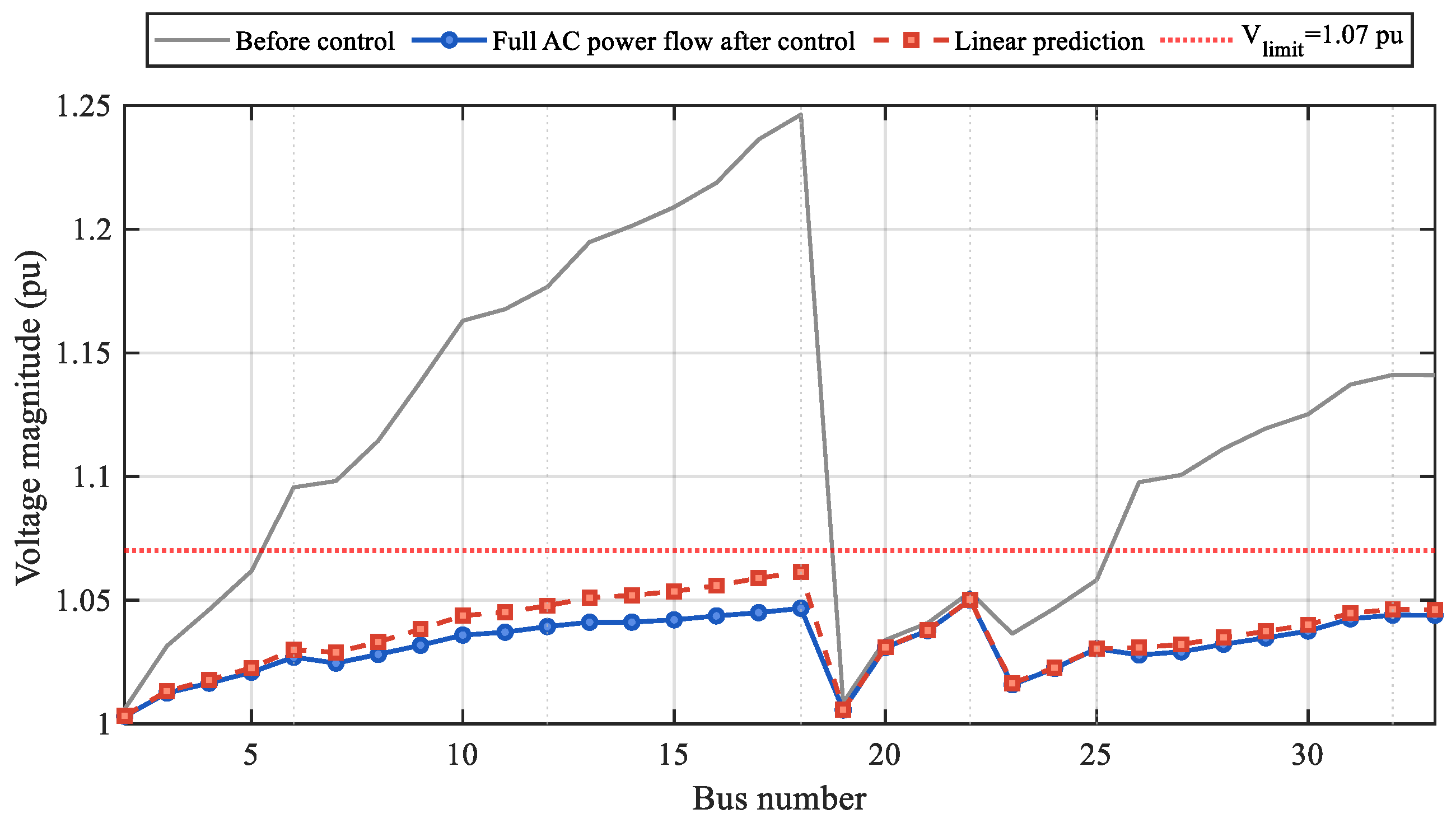
To verify the accuracy of the voltage sensitivity-based linear approximation, the post-mitigation voltage profile predicted by the linearized model is compared with that obtained from the full AC power flow at 13:00, as shown in Figure 10.
Figure 10.
Validation of linearized voltage prediction using full AC power flow.
As shown in Figure 10, the linearized prediction agrees well with the full AC power flow result. Both voltage profiles remain below the upper limit of 1.07 pu, and the maximum voltage from the AC power flow is approximately 1.052 pu, consistent with the mitigation result discussed above. This confirms that the linearized model provides sufficient accuracy around the post-mitigation operating point.
4.3.2. Comparison with the Cluster-Based Scheme
The cluster-based partitioning method, which divides PV entities into feeder-location-based clusters and assigns tasks by uniform rules, is adopted as the comparison benchmark. The mitigation task allocations of the two schemes at the representative time instant are listed in Table 2.
Table 2.
Mitigation task allocation under the two schemes at 13:00.
As shown in Table 2, the cluster-based method concentrates active power curtailment heavily on PV3, with a curtailment of 2755.71 kW, while the active power curtailments of PV1, PV4, PV5, and PV6 are all zero. Reactive power regulation is also concentrated on only three entities: PV1, PV2, and PV6. In contrast, under the proposed method, five entities bear active power curtailment tasks, with only PV4 having zero curtailment due to its extremely low responsibility share. Reactive power regulation is distributed across all six entities, resulting in a substantially more balanced overall distribution.
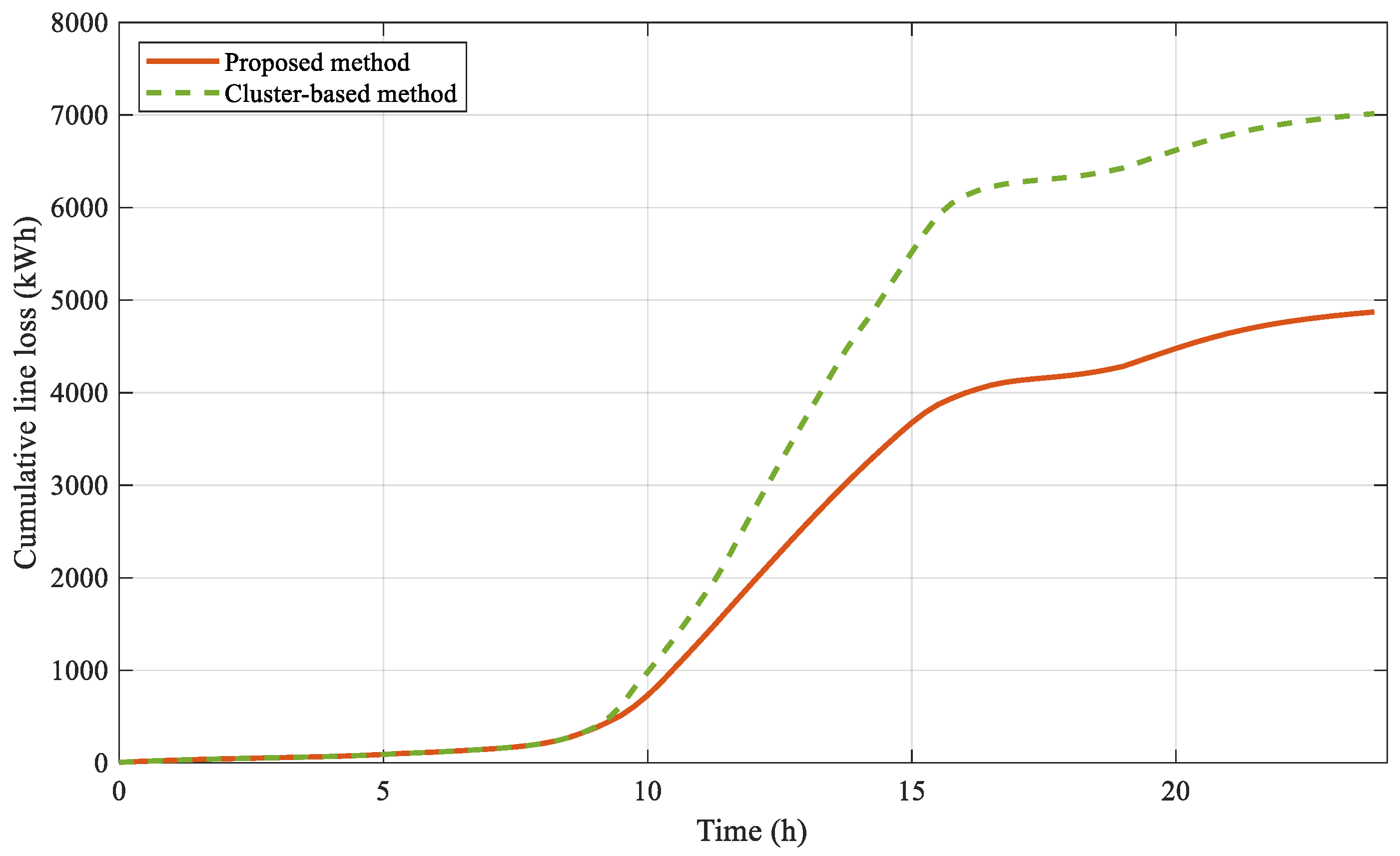
The comprehensive performance indicators of the two schemes are compared in Table 3, and the comparison of 24-h cumulative line losses over time is shown in Figure 8.
Table 3.
Overall performance comparison between the two schemes.
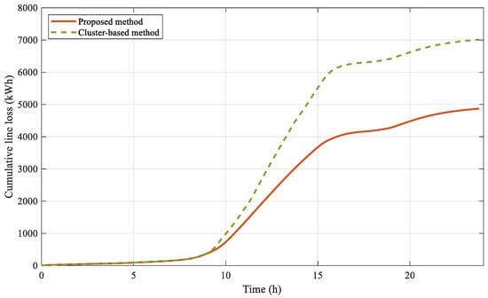
Both schemes achieve zero violated nodes after mitigation, confirming that voltage safety is ensured in both cases. The maximum nodal voltage under the proposed method is 1.052 pu, slightly lower than 1.057 pu under the cluster-based method. In terms of system losses, the proposed method achieves a typical-time-instant loss of 607.81 kW, a reduction of 38.4% compared with the cluster-based method. The 24-h cumulative line loss is 4872.42 kWh, representing a reduction of 30.6%. Figure 11 further shows that the line losses of the two methods are essentially equivalent before 10:00, after which the cumulative line loss of the cluster-based method increases at an accelerated rate, with the differences primarily concentrated during high PV output periods. Regarding PV curtailment and fairness, the total PV curtailment rate of the proposed method is 16.51%, higher than the 11.92% of the cluster-based method. However, the fairness deviation is 2.39 × 10⁻⁵, approximately 89% lower than the 2.20 × 10⁻⁴ of the cluster-based method. The cluster-based method curtails less PV power but relies on concentrated reactive regulation, driving higher line losses during peak-output hours. The proposed method accepts greater curtailment in exchange for more distributed task allocation and substantially lower losses.
Figure 11.
Comparison of 24-h cumulative line losses.
To further assess the robustness of the proposed method under varying operating conditions, a parameter sensitivity analysis is conducted in the following section.
4.4. Parameter Sensitivity Analysis
4.4.1. PV Output Multiplier Sensitivity
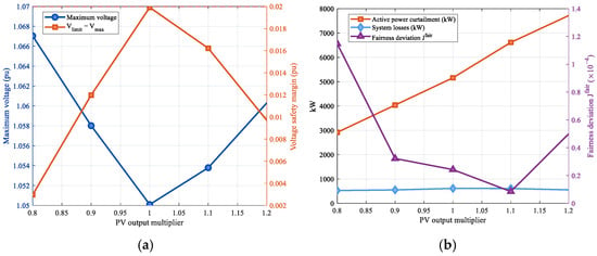
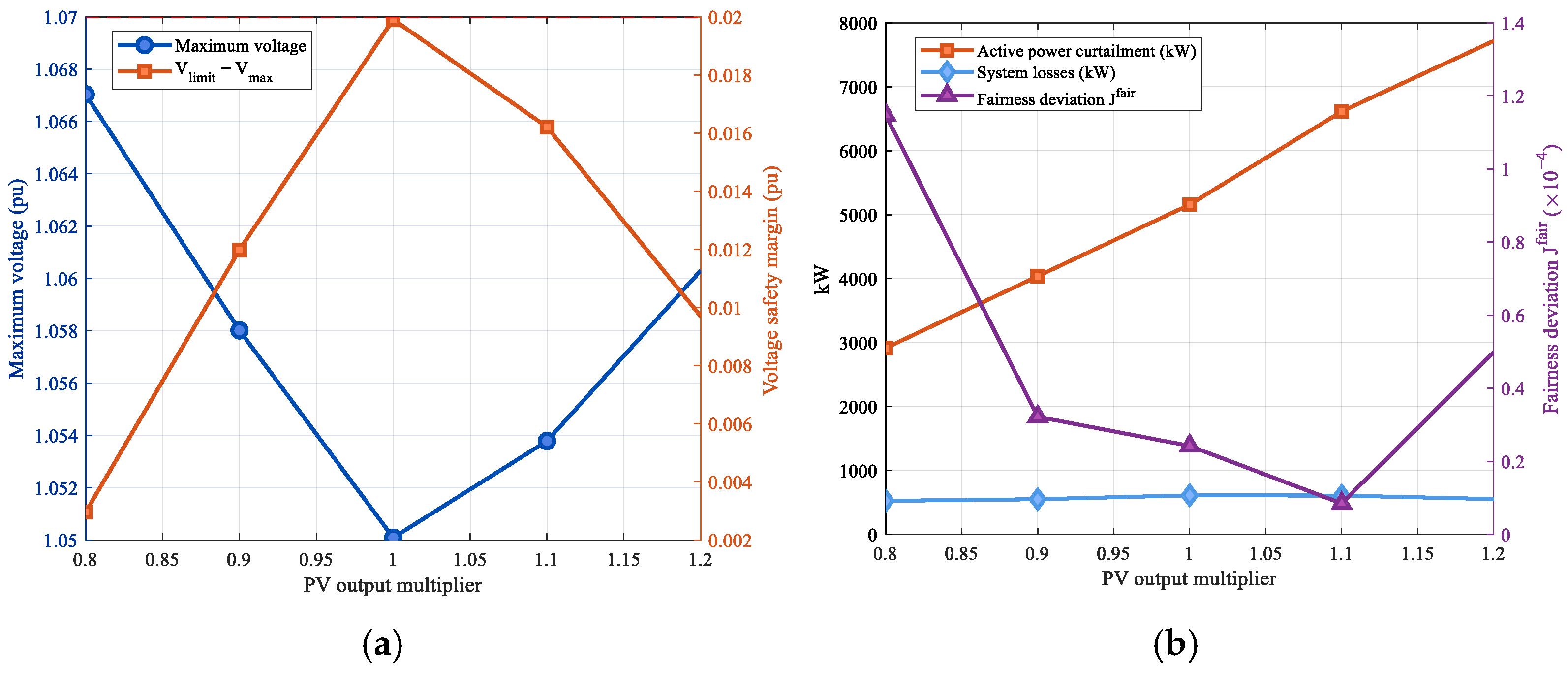
The actual PV output level is affected by meteorological conditions such as irradiance and may deviate significantly from typical-day data, which directly impacts the degree of system overvoltage and the scale of mitigation tasks. To verify the adaptability of the proposed method under different PV output conditions, five output multiplier levels of 0.8, 0.9, 1.0, 1.1, and 1.2 are set, and the variation patterns of mitigation effectiveness with PV output fluctuations are analyzed. The results are shown in Figure 12.
Figure 12.
Sensitivity of mitigation performance to PV output multiplier at 13:00. (a) Voltage safety metrics. (b) Curtailment, losses, and fairness deviation.
In terms of voltage safety, when the output multiplier varies in the range of 0.8 to 1.2, the maximum voltage after mitigation consistently remains below 1.07 pu, fluctuating between 1.050 and 1.061 pu. This demonstrates that the proposed method can effectively eliminate overvoltage under various PV output levels. The voltage safety margin is largest at the 0.9 multiplier and smallest at the 1.0 multiplier, with an overall variation range of 0.002 to 0.02 pu.
In terms of economy and fairness, the active power curtailment exhibits a monotonically positive correlation with the output multiplier, increasing monotonically from approximately 2900 kW to approximately 7700 kW, reflecting the pattern that overvoltage mitigation demand increases significantly with higher PV output. System losses are less affected by the multiplier, remaining at approximately 550 kW, indicating that the proposed method can effectively control losses under various output scenarios. The fairness deviation exhibits a non-monotonic trend, first decreasing and then increasing, reaching its minimum near the 1.1 multiplier. This is because the responsibility share distribution among entities is more uniform at this multiplier, achieving the best coordination effect among optimization objectives. These results confirm that the proposed method is robust to PV output variations.
4.4.2. Joint Sensitivity of Weight Parameters
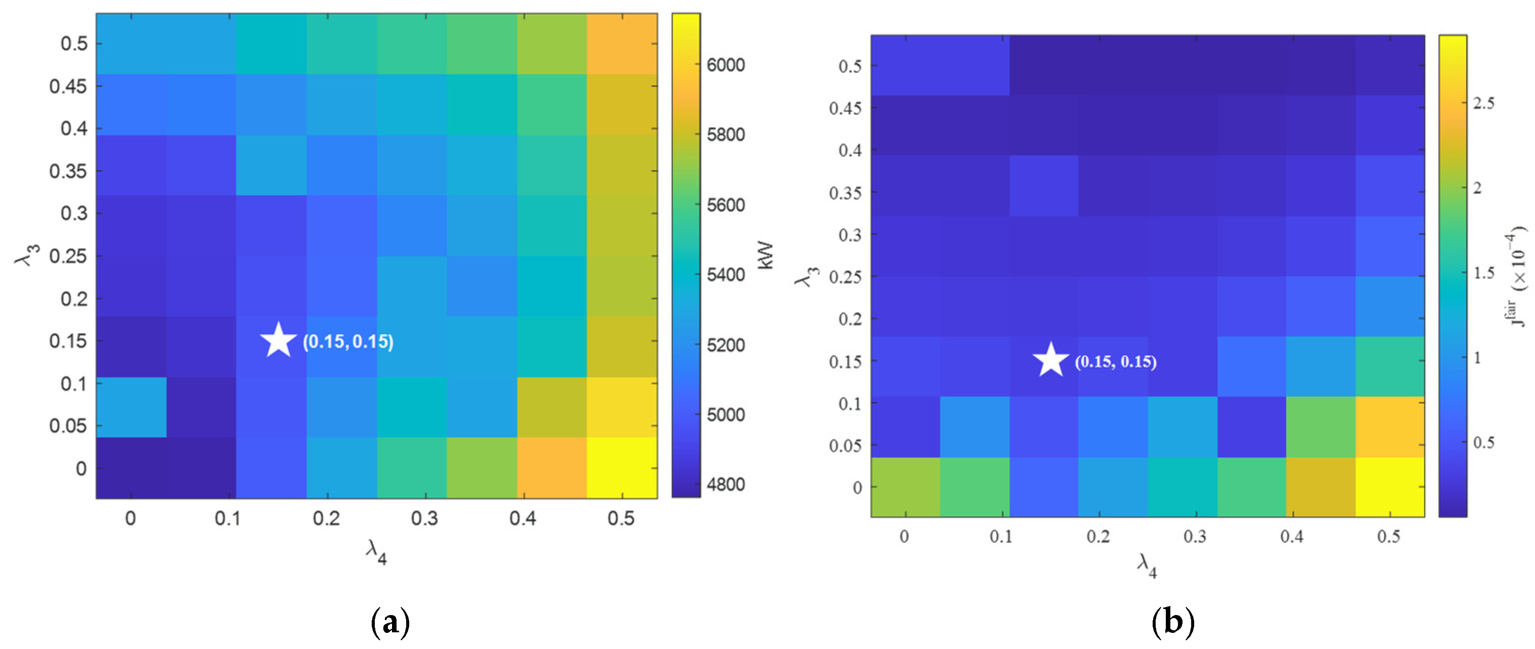
Since λ1 and λ2 correspond to intuitive operational indicators and are fixed by engineering experience, the analysis focuses on λ3 and λ4, which jointly govern the trade-off among fairness and task-allocation consistency. Their influence is assessed by varying both within [0, 0.5].
The heat map results are shown in Figure 13.
Figure 13.
Joint sensitivity heat maps of λ3–λ4 at 13:00. (a) Active power curtailment. (b) Fairness deviation.
As shown in Figure 13a, the active power curtailment is more sensitive to changes in λ4, exhibiting a significantly positive correlation with λ4. When λ4 is large, the model imposes a heavier penalty on task-allocation deviation, driving the optimization to increase active power curtailment to satisfy the task-allocation constraint, with the curtailment reaching a maximum of approximately 6500 kW. When λ4 is small, the curtailment is concentrated within the range of 4800 to 5200 kW. In comparison, the influence of λ3 on active power curtailment is relatively limited.
As shown in Figure 13b, the fairness deviation is primarily governed by λ3, exhibiting a significantly negative correlation. As λ3 increases, the fairness deviation decreases continuously, indicating that increasing the fairness deviation weight effectively drives the task allocation toward a more balanced distribution. The influence of λ4 on fairness deviation is notably weaker, suggesting that the task-allocation deviation constraint and the fairness objective are relatively independent. Considering both dimensions, when λ3 = λ4 = 0.15, the active power curtailment is moderate and the fairness deviation is at a relatively low level. This parameter combination is selected as the baseline configuration in this paper.
4.4.3. Single-Parameter Sensitivity of the Fairness Deviation Weight
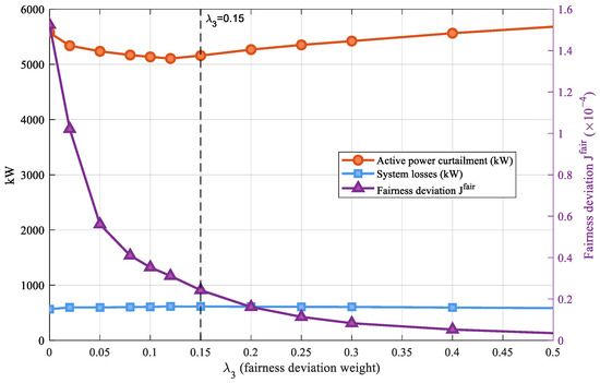
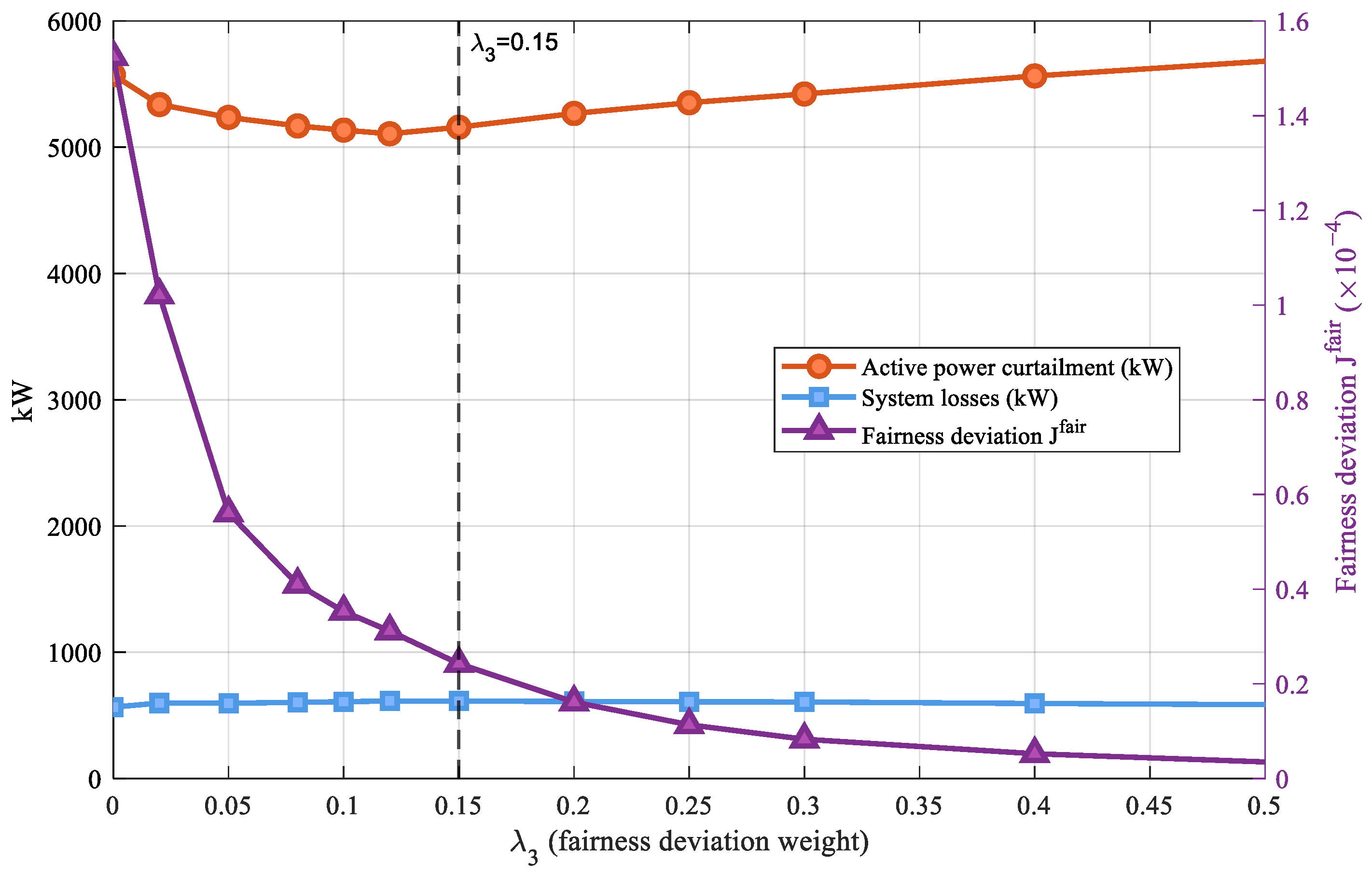
The sensitivity analysis in Section 4.4.2 demonstrates that λ3 is the dominant parameter affecting the fairness deviation. To further clarify the operational boundary and optimal value range of this weight, λ4 is fixed at 0.15, and a refined parametric analysis is conducted for λ3 within the range [0, 0.5]. The results are shown in Figure 14.
Figure 14.
Single-parameter sensitivity to λ3.
As shown in Figure 14, when λ3 increases from 0 to 0.15, the fairness deviation drops rapidly from approximately 1.5 × 10⁻⁴ to approximately 9 × 10⁻⁶, a reduction exceeding 90%. This indicates that moderately introducing a fairness deviation penalty can produce significant and rapid improvement in the balance of task allocation. Meanwhile, the active power curtailment decreases only slightly, and the system losses remain virtually unaffected, demonstrating that the fairness improvement in this range does not come at the cost of increased PV curtailment or higher line losses. When λ3 exceeds 0.15, the fairness deviation levels off, and further increases in λ3 yield very limited additional improvement in fairness. However, the active power curtailment shows a slight increase, indicating that an excessively high fairness deviation weight introduces unnecessary additional curtailment with diminishing marginal improvement. Overall, λ3 = 0.15 marks the end of the rapid descent phase of the fairness deviation curve, achieving substantial fairness improvement at minimal curtailment cost without triggering diminishing returns. This value is therefore selected as the baseline parameter.
5. Conclusions
This paper proposes a responsibility-driven overvoltage mitigation method for distribution networks with high distributed PV penetration. The TOPSIS-based reverse power flow quota provides a comprehensive reflection of each entity’s utilization of the voltage safety margin. The Shapley value method quantifies overvoltage responsibility by capturing network coupling and marginal contribution differences that capacity-based or equal-share allocation cannot reveal. The active–passive responsibility mapping mechanism translates responsibility shares into differentiated tasks for active power curtailment and reactive power regulation. Furthermore, a multi-objective optimization model is developed to balance line losses, PV curtailment, fairness, and task-allocation consistency.
Case studies on the IEEE 33-bus system demonstrate that the Shapley value method effectively reveals network coupling differences among entities, as indicated by the significant divergence between responsibility shares and quota proportions. The active–passive responsibility mapping mechanism ensures that the allocation ratios of each entity’s active and reactive power tasks align with its regulatory characteristics. The proposed method reduces the maximum network voltage from 1.25 pu to 1.052 pu and eliminates all overvoltage violations in the studied case. Compared with the cluster-based scheme, the 24-h cumulative line loss is reduced by 30.6%, and the fairness deviation is significantly lowered.
The case study is limited to a radial network with six entities; therefore, scalability to larger systems warrants further investigation. Further verification is still needed for transformer areas with more controllable entities, especially considering the increasing coalition-enumeration complexity of the Shapley value method. In addition, the cluster-based benchmark represents only a topology-based rule allocation scheme, and comparisons with other responsibility-based non-Shapley schemes should be further investigated. Practical deployment may also be affected by communication delays, measurement availability, inverter response limits, and coordination mechanisms between distribution operators and PV entities. These issues will be addressed in future work.
Author Contributions
Conceptualization, T.Y. and Q.C.; methodology, T.Y. and Q.C.; software, Q.C. and S.B.; validation, T.Y., Q.C., S.B., D.W., B.C., D.L. and H.W.; formal analysis, T.Y., Q.C., S.B., D.W., B.C., D.L. and H.W.; investigation, Q.C.; resources, Q.C. and B.C.; data curation, T.Y., Q.C., S.B., D.W., B.C., D.L. and H.W.; writing—original draft preparation, T.Y., Q.C., S.B., D.W., B.C., D.L. and H.W.; writing—review and editing, T.Y., Q.C., S.B., D.W., B.C., D.L. and H.W.; visualization, Q.C.; supervision, D.L.; project administration, T.Y.; funding acquisition, H.W. All authors have read and agreed to the published version of the manuscript.
Funding
This research was funded by the Natural Science Foundation of Jiangsu Province, grant number BK20251067.
Institutional Review Board Statement
Not applicable.
Informed Consent Statement
Not applicable.
Data Availability Statement
The original contributions presented in this study are included in the article. Further inquiries can be directed to the corresponding author.
Conflicts of Interest
The authors declare no conflicts of interest.
Appendix A
To examine the sensitivity of quota allocation to the multi-criteria evaluation method, entropy-weighting and eigenvector-based weighting are compared with TOPSIS. All three methods are applied to the original matrix of power-flow impact and voltage-sensitivity indicators, and the resulting quotas are evaluated through the same responsibility quantification and mitigation optimization procedure. The comparison uses Quota CV (coefficient of variation), , , line loss, and .
Table A1.
Comparison of multi-criteria quota evaluation methods at 13:00.
As shown in Table A1, all three methods obtain voltage-feasible results with similar maximum voltages. TOPSIS yields the lowest Quota CV, , and , indicating lower quota dispersion, curtailment effort, and fairness deviation. Although entropy-weighting and eigenvector-based weighting lead to slightly lower line losses, they result in larger quota dispersion and higher fairness deviation. Therefore, TOPSIS is adopted as a balanced quota evaluation method in this study.
Appendix B
Figure A1.
Convergence performance of WOA.
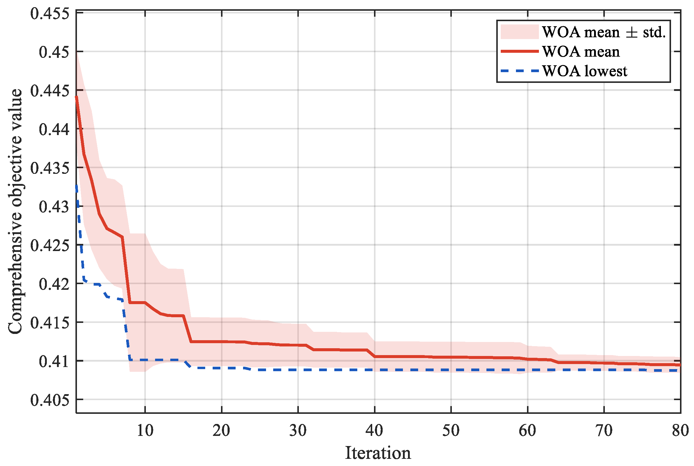
As shown in Figure A1, the objective value decreases rapidly in the early iterations and gradually stabilizes after approximately 40 iterations, indicating stable convergence of WOA.
Table A2.
Convergence and reproducibility comparison of WOA, PSO and NSGA-II.
As shown in Table A2, WOA reaches both the 5% and 1% convergence gaps earlier than PSO and NSGA-II. For solvers that do not reach the specified convergence gap within 80 iterations, the iteration number is recorded as the maximum iteration number of 80. WOA also obtains the smallest standard deviation of the final objective value, indicating better convergence speed and repeatability in the studied optimization problem.
References
- Haque, M.M.; Wolfs, P. A review of high PV penetrations in LV distribution networks: Present status, impacts and mitigation measures. Renew. Sustain. Energy Rev. 2016, 62, 1195–1208. [Google Scholar] [CrossRef] [Scilit]
- Ali, M.S.; Haque, M.M.; Wolfs, P. A review of topological ordering based voltage rise mitigation methods for LV distribution networks with high levels of photovoltaic penetration. Renew. Sustain. Energy Rev. 2019, 103, 463–476. [Google Scholar] [CrossRef] [Scilit]
- Chaudhary, P.; Rizwan, M. Voltage regulation mitigation techniques in distribution system with high PV penetration: A review. Renew. Sustain. Energy Rev. 2018, 82, 3279–3287. [Google Scholar] [CrossRef] [Scilit]
- Demirok, E.; González, P.C.; Frederiksen, K.H.B.; Sera, D.; Rodríguez, P.; Teodorescu, R. Local reactive power control methods for overvoltage prevention of distributed solar inverters in low-voltage grids. IEEE J. Photovolt. 2011, 1, 174–182. [Google Scholar] [CrossRef] [Scilit]
- Pompodakis, E.E.; Drougakis, I.A.; Lelis, I.S.; Alexiadis, M.C. Photovoltaic systems in low-voltage networks and overvoltage correction with reactive power control. IET Renew. Power Gener. 2016, 10, 410–417. [Google Scholar] [CrossRef] [Scilit]
- Li, C.; Disfani, V.R.; Haghi, H.V.; Kleissl, J. Coordination of OLTC and smart inverters for optimal voltage regulation of unbalanced distribution networks. Electr. Power Syst. Res. 2020, 187, 106498. [Google Scholar] [CrossRef] [Scilit]
- Wang, Y.; Tan, K.T.; Peng, X.Y.; So, P.L. Coordinated control of distributed energy-storage systems for voltage regulation in distribution networks. IEEE Trans. Power Deliv. 2016, 31, 1132–1141. [Google Scholar] [CrossRef] [Scilit]
- Zeraati, M.; Golshan, M.E.H.; Guerrero, J.M. Distributed control of battery energy storage systems for voltage regulation in distribution networks with high PV penetration. IEEE Trans. Smart Grid 2018, 9, 3582–3593. [Google Scholar] [CrossRef] [Scilit]
- Zeraati, M.; Golshan, M.E.H.; Guerrero, J.M. A consensus-based cooperative control of PEV battery and PV active power curtailment for voltage regulation in distribution networks. IEEE Trans. Smart Grid 2019, 10, 670–680. [Google Scholar] [CrossRef] [Scilit]
- Sharma, S.; Verma, A.; Panigrahi, B.K. Robustly coordinated distributed voltage control through residential demand response under multiple uncertainties. IEEE Trans. Ind. Appl. 2021, 57, 4042–4058. [Google Scholar] [CrossRef] [Scilit]
- Camilo, F.M.; Castro, R.; Almeida, M.E.; Pires, V.F. Assessment of overvoltage mitigation techniques in low-voltage distribution networks with high penetration of photovoltaic microgeneration. IET Renew. Power Gener. 2018, 12, 649–656. [Google Scholar] [CrossRef] [Scilit]
- Xu, Y.; Dong, Z.Y.; Zhang, R.; Hill, D.J. Multi-timescale coordinated voltage/Var control of high renewable-penetrated distribution systems. IEEE Trans. Power Syst. 2017, 32, 4398–4408. [Google Scholar] [CrossRef] [Scilit]
- Zhang, C.; Xu, Y.; Dong, Z.Y.; Ravishankar, J. Three-stage robust inverter-based voltage/Var control for distribution networks with high-level PV. IEEE Trans. Smart Grid 2019, 10, 782–793. [Google Scholar] [CrossRef] [Scilit]
- Xu, R.; Zhang, C.; Xu, Y.; Dong, Z.Y. Rolling horizon based multi-objective robust voltage/VAR regulation with conservation voltage reduction in high PV-penetrated distribution networks. IET Gener. Transm. Distrib. 2019, 13, 1621–1629. [Google Scholar] [CrossRef] [Scilit]
- Ricciardi, T.R.; Petrou, K.; Franco, J.F.; Ochoa, L.F. Defining customer export limits in PV-rich low voltage networks. IEEE Trans. Power Syst. 2019, 34, 87–97. [Google Scholar] [CrossRef] [Scilit]
- Gebbran, D.; Mhanna, S.; Ma, Y.; Chapman, A.C.; Verbič, G. Fair coordination of distributed energy resources with Volt-Var control and PV curtailment. Appl. Energy 2021, 286, 116546. [Google Scholar] [CrossRef] [Scilit]
- Luo, C.; Wu, H.; Zhou, Y.; Qiao, Y.; Cai, M. Network partition-based hierarchical decentralised voltage control for distribution networks with distributed PV systems. Int. J. Electr. Power Energy Syst. 2021, 130, 106929. [Google Scholar] [CrossRef] [Scilit]
- Emarati, M.; Barani, M.; Farahmand, H.; Aghaei, J.; Crespo del Granado, P. A two-level over-voltage control strategy in distribution networks with high PV penetration. Int. J. Electr. Power Energy Syst. 2021, 130, 106763. [Google Scholar] [CrossRef] [Scilit]
- Sekizaki, S.; Nishizaki, I.; Hayashida, T. Cooperative voltage management by demand resources and fair payoff allocation for distribution systems. Int. J. Electr. Power Energy Syst. 2023, 145, 108696. [Google Scholar] [CrossRef] [Scilit]
- Antoniadou-Plytaria, K.E.; Kouveliotis-Lysikatos, I.N.; Georgilakis, P.S.; Hatziargyriou, N.D. Distributed and decentralized voltage control of smart distribution networks: Models, methods, and future research. IEEE Trans. Smart Grid 2017, 8, 2999–3008. [Google Scholar] [CrossRef] [Scilit]
- Tan, X.; Lie, T.T. Application of the Shapley value on transmission cost allocation in the competitive power market environment. IEE Proc.-Gener. Transm. Distrib. 2002, 149, 15–20. [Google Scholar] [CrossRef] [Scilit]
- Sharma, S.; Abhyankar, A.R. Loss allocation of radial distribution system using Shapley value: A sequential approach. Int. J. Electr. Power Energy Syst. 2017, 88, 33–41. [Google Scholar] [CrossRef] [Scilit]
- Pourahmadi, F.; Dehghanian, P. A game-theoretic loss allocation approach in power distribution systems with high penetration of distributed generations. Mathematics 2018, 6, 158. [Google Scholar] [CrossRef] [Scilit]
- Rahmani-Dabbagh, S.; Sheikh-El-Eslami, M.K. Risk-based profit allocation to DERs integrated with a virtual power plant using cooperative game theory. Electr. Power Syst. Res. 2015, 121, 368–378. [Google Scholar] [CrossRef] [Scilit]
- Rahmani-Dabbagh, S.; Sheikh-El-Eslami, M.K. A profit sharing scheme for distributed energy resources integrated into a virtual power plant. Appl. Energy 2016, 184, 313–328. [Google Scholar] [CrossRef] [Scilit]
- Yu, K.; Tang, X.; Chen, X.; Bu, L.; Hua, H.; Ding, Y.; Shen, J. Allocation Method of Overvoltage Responsibility in Distribution Network with High Proportion Distributed Photovoltaic. Proc. CSEE 2023, 43, 9535–9546. [Google Scholar] [CrossRef]
- Singh, D.; Singh, D.; Verma, K.S. Multiobjective Optimization for DG Planning with Load Models. IEEE Trans. Power Syst. 2009, 24, 427–436. [Google Scholar] [CrossRef] [Scilit]
- Niknam, T.; Zare, M.; Aghaei, J. Scenario-Based Multiobjective Volt/Var Control in Distribution Networks Including Renewable Energy Sources. IEEE Trans. Power Deliv. 2012, 27, 2004–2019. [Google Scholar] [CrossRef] [Scilit]
- Zhang, C.; Xu, Y.; Dong, Z.Y.; Zhang, R. Multi-Objective Adaptive Robust Voltage/VAR Control for High-PV Penetrated Distribution Networks. IEEE Trans. Smart Grid 2020, 11, 5288–5300. [Google Scholar] [CrossRef] [Scilit]

Disclaimer/Publisher’s Note: The statements, opinions and data contained in all publications are solely those of the individual author(s) and contributor(s) and not of MDPI and/or the editor(s). MDPI and/or the editor(s) disclaim responsibility for any injury to people or property resulting from any ideas, methods, instructions or products referred to in the content. |
© 2026 by the authors. Licensee MDPI, Basel, Switzerland. This article is an open access article distributed under the terms and conditions of the Creative Commons Attribution (CC BY) license.