


Abstract
Night-time low temperature remains a major constraint on thermal stability, crop safety and energy-efficient operation in winter solar greenhouses, especially when heat release and auxiliary heating are triggered only after the indoor temperature has approached a low temperature threshold. This study developed a temperature prediction-based active–passive heat storage and release system integrating Internet of Things monitoring, liquid neural network (LNN)-based multi-horizon temperature forecasting, heat storage and release circulation, and decision-making control. The LNN achieved the best forecasting performance among the tested models, with MAE/RMSE values of 0.620/0.775, 0.683/0.854 and 0.758/0.948 °C for 12 h, 24 h and 48 h forecasts, respectively, and was embedded into the system for prediction-assisted operation. A continuous 30-day winter test was conducted in two consecutive stages: heat storage and release without predictive control (HS-NPC, days 1–15) and with prediction-assisted operation (HS-PC, days 16–30). During the consecutive-stage winter test, HS-PC showed higher daily minimum indoor temperature and night-time mean temperature than HS-NPC by 1.92 °C and 4.29 °C, respectively, while reducing daily exposure below 13 °C and 10 °C by 55.0% and 98.2%. Stage-based equivalent input-energy evaluation indicated reductions of 17.1% and 34.3% for HS-NPC and HS-PC relative to the corresponding TG reference periods, respectively. Because HS-NPC and HS-PC were tested in consecutive weather windows rather than in fully synchronized parallel experiments, these improvements should be interpreted as stage-based operational benefits supported by the TG reference and outdoor environmental statistics, rather than as completely weather-independent causal effects. These results indicate that integrating temperature forecasting with heat storage and release regulation can improve low-temperature buffering and energy-saving operation in winter solar greenhouses, while further synchronized or weather-normalized validation is still needed.
1. Introduction
Night-time low temperature in winter is a major constraint on safe crop production and energy-efficient operation in solar greenhouses. For thermophilic crops such as tomato, low temperature can impair photosynthesis, root uptake, floral development and fruit formation, while also increasing the demand for auxiliary night-time heating [1]. With the development of protected agriculture towards low-carbon production, energy saving, and intelligent regulation, greenhouse climate control is no longer limited to maintaining a suitable temperature. It increasingly requires the coordinated optimization of low-temperature risk prevention, heat storage utilization and equipment operation. Zhang et al. reported that energy-efficient greenhouse operation requires integrated improvements in structural insulation, equipment control, heat storage and energy management [2]. Recent studies on cold-region facility agriculture and Gobi solar greenhouses further indicate that energy-saving technologies and energy-related cost control are key factors for sustainable greenhouse production [3,4]. Therefore, improving the utilization of stored solar heat is a critical issue for winter thermal regulation and energy-saving operation in solar greenhouses.
Solar greenhouses capture solar radiation through the transparent front roof and store heat in the wall, soil, rear roof and thermal insulation structures, thereby reducing night-time heat loss. During the daytime, solar radiation raises the temperature of indoor air, walls and soil; at night or under cloudy, snowy and cold-wave conditions, heat loss through the envelope increases and indoor temperature can decline rapidly. Greenhouse temperature dynamics are jointly affected by structural design, covering materials, external meteorological conditions and energy inputs [5]. Heat storage and release technologies have therefore been widely applied to improve night-time thermal stability. Passive heat storage mainly relies on walls, soil, water bodies and phase-change materials, whereas active systems use solar collectors, heat storage tanks, circulation pipelines, floor heating pipes and control devices to collect, transfer, store and release heat. Lu et al. developed and verified a thermal performance model for an active heat storage and release system [6]; Xu et al. proposed an active solar water wall for greenhouse heating [7]; Wang et al. used a water cycle system to store surplus daytime air thermal energy and release it through water circulation in a Chinese-type solar greenhouse [8]; and Xia et al. designed an active solar heat storage and release system for high-latitude and cold regions [9]. These studies demonstrate the potential of active heat storage and release to improve greenhouse night-time thermal environments. Related studies have also shown that system configuration, phase-change materials and storage media influence heat storage and release performance [10,11,12,13].
However, the practical performance of active–passive heat storage and release systems depends not only on structural design and heat storage capacity, but also on whether heat storage, heat release and auxiliary heating can be matched with forthcoming low-temperature processes. Existing operation methods mostly rely on fixed schedules, manual experience or real-time temperature thresholds. Fixed-schedule control is poorly adapted to weather variability, while real-time threshold-based control starts the system only after the indoor temperature has approached or fallen below a predefined value. For systems with strong thermal inertia, daytime heat storage intensity determines the heat available for night-time release, and the timing of night-time heat release directly affects temperature stability and energy consumption. Without prior information on future cooling processes, the system may suffer from insufficient heat storage, delayed heat release, untimely auxiliary heating or ineffective circulation. Previous studies on greenhouse energy-saving control and environmental optimization have shown that control strategies should coordinate crop environmental requirements, equipment operating states and energy consumption rather than relying on a single temperature threshold [14,15].
Temperature forecasting provides a basis for anticipatory operation of heat storage and release systems. Process-based greenhouse climate models describe heat exchange among greenhouse air, walls, soil, crops and covering materials and can provide mechanistic interpretation [16,17]. However, such models often require detailed parameters and may have limited adaptability across operating conditions. With the accumulation of Internet of Things-based monitoring data, data-driven models have become effective tools for learning nonlinear greenhouse temperature dynamics from indoor and outdoor environmental variables. Neural network, deep learning and other data-driven methods have been applied to greenhouse air temperature forecasting and microclimate modeling, demonstrating their suitability for nonlinear greenhouse environmental prediction [18,19,20,21]. Meanwhile, model predictive control studies have shown that future state information can be used to coordinate environmental regulation targets and energy consumption in agricultural systems with nonlinearity, time delay and multiple constraints [22,23,24,25,26]. Therefore, the value of temperature forecasting should not be evaluated only by offline error metrics such as MAE and RMSE, but also by its ability to support low-temperature risk identification, heat release timing and auxiliary heating decisions.
Winter air temperature in solar greenhouses is affected by solar radiation, outdoor meteorological conditions, heat storage and release by the envelope, soil thermal inertia, equipment operation and crop transpiration. These processes exhibit strong nonlinearity, time lag and multi-timescale characteristics. Liquid neural networks (LNNs), which use learnable time constants and continuous-time state updates to describe dynamic systems, are suitable for representing complex temporal processes [27]. Extreme Gradient Boosting (XGBoost), with strong nonlinear fitting capacity and engineering applicability, can serve as a representative ensemble tree model for comparison [28]. Introducing an LNN into temperature forecasting for active–passive heat storage and release systems, and comparing it with GRU and XGBoost, can help identify a forecasting module capable of providing stable future temperature trajectories for system operation.
Based on the above analysis, this study designed a temperature prediction-based active–passive heat storage and release system for solar greenhouses. The system integrates Internet of Things-based environmental monitoring, LNN-based multi-horizon indoor air temperature forecasting, heat storage and release circulation, and decision-making control. Future minimum temperature, timing of low-temperature occurrence, cooling rate and low-temperature duration are extracted from predicted temperature sequences and converted into operating decisions for circulating heat release and auxiliary electric heating. By embedding future temperature information into the heat storage and release system, greenhouse thermal regulation is shifted from real-time threshold response to anticipatory regulation oriented towards forthcoming low-temperature processes. Compared with previous studies that separately addressed heat storage hardware, greenhouse temperature forecasting or predictive control, the novelty of this study lies in coupling multi-horizon LNN-based temperature forecasts with an active–passive heat storage and release prototype and translating forecast-derived low-temperature-process variables into executable heat release and auxiliary heating decisions. Thus, the contribution is not the independent proposal of heat storage, forecasting or predictive control, but their integrated implementation and operational evaluation for anticipatory low-temperature regulation in a winter solar greenhouse. The objectives of this study were to design and test a temperature prediction-based active–passive heat storage and release system, evaluate the multi-horizon forecasting performance of the LNN relative to GRU and XGBoost, and examine the stage-based operational performance of prediction-assisted operation in terms of low-temperature buffering, auxiliary heating demand and equivalent input-energy consumption during a continuous winter operation test.
2. Materials and Methods
2.1. System Design and Operation
To meet the requirements for night-time low-temperature buffering and energy-efficient heating in winter solar greenhouses, a temperature prediction-based active–passive heat storage and release system was designed in this study. The system integrates passive heat storage by the greenhouse wall, soil and heat storage media with solar heat collection, water-tank heat storage, pipeline-based circulating heat release, auxiliary electric heating, and prediction-based decision-making control. It therefore forms a thermal environment regulation process characterized by daytime heat storage, night-time heat release, and supplementary heating under low-temperature conditions. The physical view and structural drawing of the system main body are shown in Figure 1, and the overall system structure is shown in Figure 2. The main technical parameters of the system are listed in Table 1.
Figure 1.
Physical view and structural drawing of the temperature prediction-based active–passive heat storage and release system. Note: (a) Physical view of the active–passive heat storage and release system; (b) structural drawing of the active–passive heat storage and release system: 1, exhaust valve; 2, supporting beam; 3, solar collector; 4, valve; 5, water inlet; 6, return water outlet; 7, control cabinet; 8, base.
Figure 2.
Overall structure of the active–passive heat storage and release system.
Table 1.
Main components and parameters.
The active–passive heat storage and release system consists of three functional modules: a passive heat storage module, an active heat storage and release module, and an auxiliary heating module. The passive heat storage module relies on the greenhouse wall, soil and near-surface heat storage media to absorb solar heat during the daytime and release it slowly at night through temperature gradients. The active heat storage and release module consists of solar collectors, a heat storage water tank, circulating pumps, solenoid valves, check valves, circulation pipelines and floor heating pipelines. This module enables the active collection, transfer, storage and release of heat. The auxiliary heating module consists of an auxiliary electric heating device and its control circuit, and provides additional heat when stored heat release is insufficient or when the greenhouse is exposed to a high low-temperature risk. Through the coordinated operation of these modules, surplus solar energy during the daytime can be converted into dispatchable heat for night-time use, thereby improving the thermal stability of the greenhouse during low-temperature periods. The detailed heat storage and release processes are shown in Figure 3.
Figure 3.
Heat storage and release processes of the active–passive heat storage and release system. Note: (a) daytime passive heat storage process in the TG; (b) daytime active–passive heat storage process in the heat storage and release greenhouse; (c) night-time passive heat release process in the traditional greenhouse; (d) night-time active–passive heat release process in the heat storage and release greenhouse.
The control device consists of a temperature acquisition unit, a control cabinet, a circulating pump drive unit, a solenoid valve control unit and an auxiliary electric heating control unit. The temperature acquisition unit records the operating states of the solar collectors, heat storage water tank, circulation pipelines and greenhouse air. The control cabinet generates system operation commands based on real-time temperature feedback and the prediction-assisted strategy described below. The circulating pump and solenoid valves regulate the water circulation pathway and the on–off state of the system. The auxiliary electric heating device rapidly increases the circulating water temperature during periods of evident low-temperature risk. The control device does not alter the greenhouse structure itself; instead, it regulates the timing and intensity of heat release by controlling water circulation and auxiliary electric heating.
The system operates in three typical states: daytime heat storage, night-time circulating heat release and auxiliary heating. During the daytime heat storage stage, when solar radiation increases and the solar collector temperature satisfies the operating condition, the circulating pump is activated. Circulating water flows between the solar collectors and the heat storage tank, transferring solar heat into the tank for storage. During the night-time circulating heat release stage, the circulating pump and solenoid valves are activated, and hot water from the heat storage tank flows through the circulation pipelines into the floor heating pipelines. The stored heat is then released to the near-surface air and root-zone environment of the greenhouse. During the auxiliary heating stage, when normal circulating heat release is insufficient and the greenhouse is exposed to an evident low-temperature risk, the auxiliary electric heating device is activated during circulation to rapidly increase the water temperature and improve the system response to strong night-time cooling.
This operating logic provides the physical basis for subsequent prediction-assisted operation. Under low-risk conditions, the system remains on standby and performs routine monitoring only. Under warning-risk conditions, the circulating pump and solenoid valves are activated to release stored heat through water circulation. Under evident low-temperature risk conditions, the circulating pump, solenoid valves and auxiliary electric heating device operate simultaneously, enabling combined circulating heat release and active supplementary heating. Thus, the active–passive heat storage and release system not only provides a night-time heat source, but also offers an executable hardware platform through which future temperature predictions can be translated into system operating states.
2.2. Temperature Forecasting Model
2.2.1. Data Acquisition and Preprocessing
The temperature forecasting dataset was obtained from the Internet of Things (IoT)-based monitoring system installed in a solar greenhouse at the Aksu Comprehensive Experimental Station, Xinjiang, China. The experimental greenhouse was 100 m long from east to west, 12 m wide from north to south, and 8 m high at the ridge. Cotton-core thermal insulation quilts were installed on the rear wall and front roof, and ventilation openings were arranged on the side and roof. Tomato was cultivated inside the greenhouse during the monitoring period.
To obtain representative greenhouse environmental data, indoor monitoring nodes were arranged along the east–west direction at distances of 20, 40, 60 and 80 m from the eastern end of the greenhouse. The sensors were installed at a height of 1.5 m. Soil temperature and moisture sensors were placed at a soil depth of 20 cm to record the thermal and moisture conditions near the root zone. Outdoor environmental data were collected using a compact weather station. The monitored variables included outdoor air temperature, relative humidity, photosynthetically active radiation and wind speed. The main technical parameters of the sensors are listed in Table 2, and the data acquisition and transmission process is shown in Figure 4.
Table 2.
Main technical parameters of the sensors.
Figure 4.
Schematic diagram of the IoT-based environmental data acquisition system. Solid black arrows indicate sensor data acquisition links, dashed black arrows indicate platform-level data flow, and yellow lightning arrows indicate wireless communication links.
The monitoring system consisted of an environmental perception layer, a data transmission layer and a platform application layer. The environmental perception layer collected indoor and outdoor air temperature and humidity, soil temperature and moisture, solar radiation, wind speed and CO2 concentration. The data transmission layer uploaded the data through LoRa wireless communication, an IoT gateway, and a 4G network. The platform application layer was used for data storage, visualization and export. This data chain provided continuous environmental samples for temperature forecasting and also supported the recording of system operating states and temperature responses during the operation test.
The forecasting dataset used for model development covered the period from 1 January 2025 to 31 December 2025, with a sampling interval of 30 min, yielding 17,520 samples. Greenhouse indoor air temperature was used as the prediction target, and indoor and outdoor environmental variables, together with historical and time-periodic features, which were used as model inputs to construct the 12 h, 24 h and 48 h forecasting tasks. The input variables included outdoor air temperature, outdoor relative humidity, indoor relative humidity, solar radiation, wind speed, soil moisture, CO2 concentration and historical temperature-rise information. Derived features included the indoor–outdoor temperature difference, humidity difference, lagged solar radiation, lagged outdoor air temperature, temperature change slope, temperature acceleration, and sine–cosine encodings of hour of day and day of year.
To avoid temporal information leakage, the 2025 dataset was divided chronologically into training, validation and independent test subsets at a ratio of 70%/15%/15%, rather than being randomly shuffled. The January 2026 operation-test data used for system validation were not included in model training, validation or testing. The temperature-rise feature was defined as a historical first-order temperature-difference feature within the input window, calculated from the current observed indoor air temperature and the previous observed indoor air temperature. Therefore, no future indoor temperature observation was used to construct this feature during training, testing or closed-loop inference. All sensors and the compact weather station listed in Table 2 were supplied by Shandong Renke Control Technology Co., Ltd. (Jinan, China).
Data preprocessing included time-index alignment, anomaly detection, missing-value processing and feature standardization. The continuity of the original time series and abnormal sensor records were first checked, and values that clearly violated physical constraints were removed. Historical input windows and future prediction labels were then constructed according to the forecasting horizon. Finally, the input features were standardized using the statistical parameters of the training set to reduce the influence of variables with different units and scales on model training.
2.2.2. Construction of the LNN-Based Temperature Forecasting Model
To obtain future temperature trajectories that could support the operation of the active–passive heat storage and release system, a greenhouse air temperature forecasting model based on a liquid neural network (LNN) was developed. The LNN is a class of neural network based on continuous-time state evolution. Its core mechanism is to represent the temporal evolution of internal system states through learnable time constants and state update dynamics. Greenhouse air temperature in winter solar greenhouses is affected by solar radiation, outdoor meteorological conditions, heat storage and release by the envelope, soil thermal inertia, equipment operation and crop transpiration. These processes are nonlinear, delayed and multi-timescale in nature. Therefore, the LNN was adopted as the forecasting module to capture the continuous evolution of the winter greenhouse thermal environment.
The LNN was selected because winter greenhouse air temperature is governed by nonlinear heat exchange, thermal inertia, delayed responses to solar radiation and heat release operation, and multi-time-scale interactions among indoor and outdoor environmental variables. Unlike recurrent architectures with fixed discrete hidden-state transitions, the LNN represents hidden-state evolution through continuous-time dynamics with learnable time constants, which is suitable for describing gradual thermal accumulation and delayed cooling or warming processes. In this study, the LNN was not assumed to be superior a priori; instead, it was evaluated against GRU and XGBoost under the same chronological data split and forecasting horizons.
The LNN used in this study consisted of three layers: an input layer, a continuous dynamic layer, and an output layer, as shown in Figure 5.
Figure 5.
Overall architecture of the LNN model for greenhouse air temperature forecasting. Note: T denotes the time-step dimension (i.e., the length of the historical input window), and X denotes the feature-channel dimension. ŷ is the model output, representing the predicted indoor air temperature. “Exogenous history” refers to the historical window of exogenous variables, and denotes the one-step-ahead exogenous driver produced recursively by the exogenous-variable generator. The symbol “+” indicates concatenation of ŷ and to form the input for the next-step update. H denotes the rolling forecast horizon (number of recursive steps), corresponding to the 12 h, 24 h, and 48 h prediction spans. During inference, the one-step-ahead exogenous driver is generated recursively and is not taken from observed future meteorological records. Solid arrows indicate the forward information flow, feedback arrows indicate recursive use of predicted outputs, and ellipses indicate repeated rolling prediction steps.
Input layer: At each 30 min sampling step, the input layer receives standardized multi-source environmental variables, historical temperature features and time-periodic features. These inputs are used together with the latent state representation to describe the current thermal condition and recent evolution of the greenhouse.
Continuous dynamical layer: The LNN layer is composed of 64 liquid neurons. The latent state evolves according to continuous-time dynamics with learnable time constants and recurrent connections, as described in Equations (1)–(3). This structure allows the model to represent nonlinear and delayed greenhouse temperature responses while keeping the computational form suitable for discrete-time training and rolling inference.
Output and closed-loop update: The output layer maps the updated latent state to the predicted indoor air temperature, as shown in Equation (4). During strict closed-loop rolling forecasting, the predicted indoor temperature from the previous step is combined with the recursively generated one-step-ahead exogenous driver to form the next-step input, as shown in Equation (5). Therefore, the model does not use future observed indoor temperature or future measured exogenous variables during inference.
With this design, the LNN forms a fully autonomous closed-loop forecasting system during inference: it does not rely on ground-truth observations of future indoor temperature or future exogenous ground-truth values, which more faithfully reflects model operation under real engineering deployment conditions.
During closed-loop inference, future exogenous inputs were generated recursively rather than taken from future measured records. For each exogenous variable, including outdoor air temperature, outdoor relative humidity, solar radiation, wind speed, soil moisture, CO2 concentration and indoor relative humidity, the exogenous-variable generator estimated the next-step value using the currently available value, first-order difference, 24 h diurnal lag term and time-periodic encodings of hour of day and day of year. The generated exogenous drivers were then combined with the predicted indoor air temperature and time-related features to reconstruct the next-step input window for rolling prediction. Thus, the 12 h, 24 h and 48 h forecasts used for prediction-assisted operation did not rely on observed future indoor temperature or future measured exogenous variables.
The overall computational pipeline is summarized as follows:
where h(t) denotes the continuous-time latent state vector, and hi(t) denotes the state of the i-th neuron; N is the latent-state dimension, and t is the continuous-time variable. u(t) is the continuous-time input feature vector, Win is the input-to-state weight matrix, Wrec is the recurrent weight matrix, and brec is the bias vector for the state update. α and β are the coefficients of the polynomial nonlinearity. τc is the vector of time constants, and τmin is the lower bound of the time constant (typically set to 0.1). max(τc, τmin) denotes an element-wise lower-bound constraint. h2 and h3 denote element-wise power operations. k is the discrete sampling index; ΔT is the sampling interval (30 min); hk and uk are the latent state and input feature vector at the k-th sample, respectively, where uk is the sampled counterpart of u(t) at the k-th sampling instant. clip(−hmax, hmax) is an element-wise clipping function that constrains the state to [−hmax, hmax], where hmax is the clipping threshold. ŷk+1 denotes the predicted temperature at the next sampling instant. Wout and bout are the output-layer weight matrix and bias term, respectively, and denotes the exogenous driving input at the next step generated recursively by the exogenous-variable generator.
The model was trained using the Huber loss function to reduce the influence of abnormal temperature fluctuations on parameter updates. The AdamW optimizer was used, together with learning-rate warmup, cosine annealing, gradient clipping and early stopping to improve training stability. The number of training epochs was set to 200, the batch size was 32, the initial learning rate was 1 × 10⁻³, the minimum learning rate was 1 × 10⁻⁵, and the gradient clipping threshold was 1.0. After training, the optimal model parameters were selected according to validation-set performance and then evaluated on the test set.
To support the LNN hyperparameter settings, a one-factor-at-a-time sensitivity analysis was performed for four key training parameters: the number of liquid neurons, batch size, gradient clipping threshold and learning-rate schedule. In each comparison, only the target parameter was changed, while the remaining settings were kept consistent with the adopted LNN configuration. The detailed results are provided in Table A1. The results showed that the adopted configuration, including 64 liquid neurons, a batch size of 32, a gradient clipping threshold of 1.0 and warmup combined with cosine annealing, was within a stable and high-performing parameter region.
2.2.3. Comparison Models and Evaluation Metrics
To evaluate the applicability of the LNN model for winter greenhouse temperature forecasting, gated recurrent unit (GRU) and XGBoost models were selected as comparison models. GRU represents a typical gated recurrent neural network suitable for processing sequential data with temporal dependence, whereas XGBoost represents an ensemble tree model with strong nonlinear fitting capability and engineering applicability. The GRU baseline consisted of two GRU layers with 64 hidden units and a dropout rate of 0.3, and was trained using Adam with a batch size of 32, a learning rate of 1 × 10⁻³, and a maximum of 200 epochs; the XGBoost baseline used 120 learners, a learning rate of 0.05, MaxNumSplits of 16, and MinLeafSize of 5. The three models used the same data partitioning strategy, input variables and prediction target. All model development, training, testing, statistical analysis and figure preparation were performed using MATLAB R2024a.
The forecasting performance of the three models was evaluated using mean absolute error (MAE), root mean square error (RMSE), coefficient of determination (R2) and normalized RMSE (NRMSE). MAE and RMSE were used to quantify absolute forecasting errors, whereas R2 and NRMSE were used to evaluate the consistency and scale-normalized error level of the predicted temperature trajectories. NRMSE was calculated as RMSE divided by the observed temperature range and expressed as a percentage. MAE and RMSE were calculated as follows:
where N denotes the number of samples, and and denote the predicted value and the corresponding ground-truth (measured) value of the i-th sample, respectively.
In addition to MAE and RMSE, control-oriented forecasting metrics were further calculated to evaluate whether the predicted temperature trajectories could support low-temperature risk identification and system operation decisions. For each prediction window, the minimum temperature, the timing of the minimum temperature, and the exposure duration below 13 °C and 10 °C were extracted from both the predicted and observed temperature sequences. The minimum-temperature MAE was used to evaluate the ability of the model to capture the low-temperature valley. The timing MAE of the minimum temperature was used to evaluate whether the model could identify the occurrence time of the coldest point. The duration MAEs below 13 °C and 10 °C were used to evaluate the prediction accuracy of low-temperature warning exposure and severe low-temperature risk exposure, respectively.
2.3. Control Strategy
2.3.1. Extraction of Forecast-Based Decision Variables
To embed temperature forecasts into the operation of the active–passive heat storage and release system, a prediction-assisted decision-making strategy was established based on future temperature trajectories. The strategy uses the greenhouse indoor air temperature sequences forecast by the LNN over 12 h, 24 h and 48 h horizons as inputs. From these sequences, the predicted minimum temperature, timing of low-temperature occurrence, cooling rate and low-temperature duration are extracted and then converted into three system operating states: standby, circulating heat release and auxiliary electric heating. Unlike real-time threshold-based control, which responds only to the current indoor temperature, the prediction-assisted decision-making strategy can identify low-temperature risk before it occurs, thereby providing a decision basis for advance heat release and auxiliary electric heating.
For a given forecasting horizon H, the future temperature sequence generated by the LNN at time k can be expressed as
where denotes the predicted temperature sequence over the next H steps from the current time k, and is the predicted greenhouse air temperature at the i-th future sampling step. Because the sampling interval of the model training data was 30 min, the 12 h, 24 h and 48 h forecasting horizons correspond to H = 24, H = 48 and H = 96, respectively.
The minimum temperature within the forecasting horizon is defined as and the corresponding occurrence time of the predicted minimum temperature is calculated as
where is the minimum temperature within forecasting horizon H, is the occurrence time of the predicted minimum temperature, is the current time, and is the prediction time step.
To describe the intensity of the forthcoming cooling process, the maximum cooling rate within the forecasting horizon is calculated as
where is the maximum predicted cooling rate within horizon , expressed in °C h−1. When the predicted temperature is increasing or remains approximately stable, the cooling rate is not used as a criterion for risk escalation. When the predicted temperature decreases rapidly and approaches the low temperature threshold, the cooling rate is used as an auxiliary indicator to determine whether circulating heat release or auxiliary heating should be initiated in advance.
Low-temperature duration was used to quantify the intensity of future low-temperature exposure. The predicted exposure durations below 13 °C and 10 °C were calculated as
where and are the predicted durations below 13 °C and 10 °C within the forecasting horizon, respectively; I() is an indicator function that takes a value of 1 when the condition inside the parentheses is satisfied and 0 otherwise. In this control-oriented forecasting framework, 13 °C and 10 °C were used as operational thresholds to quantify predicted low-temperature exposure. The 13 °C threshold represented low-temperature warning exposure for advance heat release preparation, whereas the 10 °C threshold represented severe low-temperature risk exposure requiring stronger intervention.
2.3.2. Low-Temperature Risk Classification and Control Actions
The low-temperature risk thresholds used in this study were defined as control-oriented operational thresholds rather than cultivar-independent physiological injury limits. Their selection considered the low-temperature sensitivity of tomato, the night-time temperature management requirements of solar greenhouses, and the response delay of the active–passive heat storage and release system. Previous studies on tomato low-temperature responses have shown that night-time low temperature can affect plant growth, photosynthesis, floral and fruit development, and yield formation [29,30]. In the present control strategy, 13 °C was used as the low-temperature warning control threshold T1. When the predicted temperature approached this level, advance heat release preparation or low-intensity circulation was required to buffer the forthcoming cooling process. The 10 °C threshold was used as the severe low-temperature risk control threshold T2. When the predicted temperature fell below this level, auxiliary electric heating was activated together with circulating heat release to strengthen the system response. Therefore, the two thresholds were used to translate predicted low-temperature risk into executable system operating states.
Based on the predicted minimum temperature, low-temperature duration and cooling rate, future low-temperature risk was classified into three levels: low risk, warning risk and severe low-temperature risk.
When , , and no rapid cooling trend is predicted within the forecasting horizon, the system is classified as being in a low-risk state. Under this condition, night-time heat release demand is low, and the system remains on standby or performs routine monitoring.
When , or , or the predicted temperature decreases rapidly within a short period and approaches T1, the system is classified as being in a warning-risk state. Under this condition, the circulating pump and solenoid valves are activated in advance, allowing heat from the storage water tank to be released through the floor heating pipelines to the near-surface air and root-zone environment of the greenhouse.
When , or , or the predicted temperature remains below 13 °C for a relatively long duration while decreasing rapidly, the system is classified as being in a severe low-temperature risk state. Under this condition, the auxiliary electric heating device is activated together with circulating heat release to increase the circulating water temperature and enhance the system response to strong cooling events.
In the multi-horizon operation strategy, the 12 h forecast is mainly used to determine the on–off states of circulating heat release and auxiliary heating for the coming night. The 24 h forecast is used for night-time low-temperature warning and heat storage demand assessment for the current day. The 48 h forecast is used to identify cross-day low-temperature trends and support advance heat storage preparation. When different forecasting horizons produce different risk levels, the highest risk level is adopted as the current operating basis to avoid missed low-temperature risk detection. The flowchart of the prediction-assisted operation strategy is shown in Figure 6.
Figure 6.
Decision-making flowchart of the heat storage and release system. Note: T1 is the low-temperature warning control threshold of 13 °C, and T2 is the severe low-temperature risk control threshold of 10 °C. Scool represents the predicted maximum cooling rate within the forecasting horizon, while and represent the predicted exposure durations below 13 °C and 10 °C, respectively. The system operating state is determined by the predicted minimum temperature, low-temperature exposure duration and cooling trend. In Module 1, the lower subplots show representative LNN-predicted indoor air temperature trajectories at different forecasting horizons: (a) 12 h prediction; (b) 24 h prediction; and (c) 48 h prediction. Arrows indicate information flow and decision transfer, ellipses indicate recursive forecasting, and colors distinguish different risk levels and control states.
To improve the reproducibility of the prediction-assisted operation strategy, the main decision rules and actuator states used in the prototype system are summarized in Table A3. In the current implementation, the predicted minimum temperature and the predicted exposure durations below 13 °C and 10 °C were used as the primary decision variables, whereas the cooling trend was used as an auxiliary criterion for advancing heat release or auxiliary heating actions when the predicted temperature approached the corresponding threshold. The controller translated the final risk level into three executable operating states: standby, circulating heat release, and circulating heat release combined with auxiliary electric heating. When multiple prediction horizons indicated different risk levels, the highest risk level was adopted to reduce the probability of missed low-temperature risk detection.
2.4. Evaluation Methods
2.4.1. Temperature Regulation Performance Evaluation
To evaluate the temperature regulation performance of the active–passive heat storage and release system, a continuous 30 d winter operation test from 1 January to 30 January 2026 was used for system validation. The test was divided into two consecutive 15 d stages according to the control strategy. During days 1–15, the system was operated without predictive control (HS-NPC), and circulating heat release and auxiliary heating were mainly triggered by the current indoor temperature threshold. During days 16–30, the system was operated with prediction-assisted control (HS-PC), and the controller adjusted heat release and auxiliary heating in advance according to the 12 h, 24 h and 48 h forecasts and the corresponding low-temperature risk level.
Because the two stages were conducted consecutively rather than as fully synchronized parallel treatments, the outdoor environmental background of the two stages was first compared before interpreting the system-performance results. The traditional greenhouse (TG), which was monitored continuously during the same period, was used as a stage-matched reference. The outdoor indicators included daily mean outdoor temperature, daily minimum outdoor temperature, night-time mean outdoor temperature, daily cumulative solar radiation, daily mean wind speed, and outdoor low-temperature degree-hours below 13 °C and 10 °C. Accordingly, the HS-PC/HS-NPC comparison was interpreted as a consecutive-stage operational evaluation supported by the TG reference and outdoor environmental statistics, rather than as a strictly weather-independent causal comparison.
HDH13 and HDH10 were used to describe the combined intensity and duration of outdoor low-temperature exposure, and were calculated as follows:
where and represent the outdoor low-temperature degree-hours below 13 °C and 10 °C on day d, respectively, expressed in °C h d−1; is the outdoor air temperature at the i-th sampling point on day d; is the sampling interval, expressed in hours; and is the number of valid sampling points on day d. Differences in outdoor environmental indicators between the two stages were tested using Welch’s t-test. These indicators were used to determine whether the HS-PC stage was conducted under evidently milder outdoor low-temperature conditions than the HS-NPC stage, thereby providing a meteorological background for interpreting the consecutive-stage operation test.
The system performance was evaluated using indoor temperature level, low-temperature exposure and temperature increase relative to TG. Temperature-level indicators included stage mean indoor temperature and stage minimum indoor temperature. Low-temperature exposure was quantified by the number of sampling points and converted exposure durations below 13 °C and 10 °C. In this control-oriented evaluation, exposure below 13 °C represented low-temperature warning exposure, whereas exposure below 10 °C represented severe low-temperature risk exposure. The temperature increase relative to TG was used to evaluate the warming contribution of the active–passive heat storage and release system under the corresponding operation stage.
For a given operation stage s, the stage mean indoor temperature was calculated as
and the stage minimum indoor temperature was calculated as
where is the mean indoor temperature during stage s; is the minimum indoor temperature during stage s; is the indoor air temperature of the active–passive heat storage and release greenhouse at the i-th sampling point during stage s; and is the number of sampling points in this stage.
The number of sampling points below 13 °C and 10 °C and the corresponding low-temperature exposure durations were calculated as follows:
where and are the numbers of sampling points with indoor temperatures below 13 °C and 10 °C during stage s, respectively; I() is an indicator function that takes a value of 1 when the condition is satisfied and 0 otherwise; and are the converted exposure durations below 13 °C and 10 °C during stage s, respectively, expressed in h; and is the sampling interval of the system operation data. In this study, was 10 min.
The mean temperature increase in the active–passive heat storage and release greenhouse relative to TG was calculated as
where is the mean temperature increase in the active–passive heat storage and release greenhouse relative to TG; is the air temperature of the active–passive heat storage and release greenhouse at the i-th sampling point; is the air temperature of TG at the i-th sampling point; and N is the total number of sampling points.
The effect of prediction-assisted operation was evaluated by comparing the two operation stages. The real-time threshold-control stage was used to represent the temperature response when system operation was triggered only by the current indoor temperature. The prediction-assisted operation stage was used to represent the operating effect after introducing future temperature trajectories and low-temperature risk classification. The comparison focused on changes in mean indoor temperature, minimum indoor temperature, exposure duration below 13 °C and exposure duration below 10 °C. A reduction in the number of sampling points below 10 °C after prediction-assisted operation indicates improved suppression of severe low-temperature risk, whereas a reduction in exposure duration below 13 °C indicates enhanced buffering capacity during the low-temperature warning stage.
2.4.2. Stage-Based Equivalent Input-Energy Evaluation
To clarify the boundary of the energy comparison, the energy evaluation was conducted on a stage-based equivalent input-energy basis. Because HS-NPC and HS-PC were operated as two consecutive 15 d stages rather than fully synchronized full-month parallel treatments, TG was used as the stage-matched conventional heating reference. HS-NPC was compared with TG during days 1–15, and HS-PC was compared with TG during days 16–30. The coal consumption of TG was converted into equivalent input energy in kWh using the lower heating value of coal, whereas the energy use of HS-NPC and HS-PC was obtained from measured electricity records during the corresponding operation stages. Therefore, the reported reduction rate represents a reduction in equivalent input-energy consumption relative to the corresponding TG reference period, rather than a comprehensive assessment of delivered heat, useful heat output, primary energy consumption, operating cost or CO2 emissions.
The equivalent input-energy consumption of TG was calculated as
where is the equivalent input-energy consumption of TG, kWh; is the coal consumption, kg; is the lower heating value of coal, MJ kg−1; and 3.6 is the conversion factor between MJ and kWh. In this study, the equivalent input-energy consumption of TG was calculated separately for the two operation stages using Equation (23). The equivalent input-energy consumption of TG was 2184 kWh during days 1–15 and 2340 kWh during days 16–30.
The stage-cumulative electricity consumption of the heat storage and release greenhouse during operation stage s was calculated as
where is the cumulative electricity consumption of the heat storage and release greenhouse in January, kWh; is the system electricity consumption on day d, kWh; D is the number of days in the statistical period; is the equivalent input-energy reduction, kWh; is the input-energy reduction rate, %; is the equivalent input-energy consumption of TG, kWh; and is the electricity consumption of the heat storage and release greenhouse. In this study, the stage-cumulative electricity consumption of HS-NPC during days 1–15 was 1811 kWh, and that of HS-PC during days 16–30 was 1538 kWh.
Overall, this evaluation compared the measured electricity consumption of HS-NPC and HS-PC with the stage-matched equivalent input-energy consumption of TG. The resulting values were used to quantify stage-based equivalent input-energy reduction under the tested operating conditions, while broader assessments of useful heat delivery, energy cost and carbon emissions were left for future work.
3. Results
3.1. Temperature Forecasting Performance
To evaluate the applicability of the temperature forecasting model for low-temperature risk identification in winter solar greenhouses, the forecasting performance of LNN, GRU and XGBoost was compared at three forecasting horizons: 12 h, 24 h and 48 h. The three models used the same input variables, training dataset and prediction target. The forecasting curves are shown in Figure 7, and the standard forecasting-performance metrics, including MAE, RMSE, NRMSE and R2, are listed in Table 3. Overall, all three models captured the basic diurnal variation in air temperature in the winter solar greenhouse, but their differences became more evident as the forecasting horizon increased. At the 12 h horizon, the predicted temperature curves of all models were close to the measured values, indicating that short-term forecasting was mainly constrained by recent thermal inertia and environmental disturbances. When the forecasting horizon was extended to 24 h and 48 h, the LNN tracked night-time cooling processes, temperature-valley positions and cross-day fluctuations more stably, whereas GRU showed amplitude deviations during some peak and valley periods and XGBoost was more prone to local trend shifts in long-horizon forecasting.
Figure 7.
Temperature forecasting curves of the three models. Note: (a) 12 h temperature forecasting; (b) 24 h temperature forecasting; (c) 48 h temperature forecasting.
Table 3.
Model performance comparison across different forecasting horizons.
Table 3 shows that the LNN achieved the lowest forecasting errors at all three horizons. At the 12 h, 24 h and 48 h horizons, the MAE/RMSE values of the LNN were 0.620/0.775 °C, 0.683/0.854 °C and 0.758/0.948 °C, respectively. The corresponding values were 0.655/0.817 °C, 0.727/0.902 °C and 0.848/1.056 °C for GRU, and 0.770/0.967 °C, 0.888/1.102 °C and 1.135/1.423 °C for XGBoost. Compared with GRU, the MAE of the LNN decreased by 5.34%, 6.05% and 10.61% at the 12 h, 24 h and 48 h horizons, respectively. Compared with XGBoost, the corresponding reductions were 19.48%, 23.09% and 33.22%, respectively. As the forecasting horizon increased from 12 h to 48 h, the errors of all three models increased; however, the error increase of the LNN was relatively smaller, indicating stronger trajectory-retention capability in medium- and long-horizon forecasting. The R2 values in Table 3 provide additional information on the consistency between predicted and observed temperature trajectories.
For prediction-assisted operation, average pointwise forecasting accuracy alone is not sufficient, because the control strategy depends more directly on the predicted low-temperature valley, its occurrence time and the duration of low-temperature exposure. Therefore, the minimum temperature, the timing of the minimum temperature, and the exposure durations below 13 °C and 10 °C were extracted from each prediction window to evaluate the control-oriented applicability of the forecasting results. The corresponding control-oriented forecasting metrics are provided in Table A2. The results showed that the LNN achieved the lowest minimum-temperature MAE at the 24 h and 48 h horizons, with values of 0.576 °C and 0.627 °C, respectively, indicating more stable estimation of the low-temperature valley under medium- and long-horizon forecasting. For the timing of the minimum temperature, the LNN generally showed lower errors, although the absolute timing error increased at the 48 h horizon. This suggests that long-horizon forecasting is more suitable for early awareness of low-temperature risk than for precisely locating the coldest point. For exposure duration below 13 °C, the LNN maintained lower errors than GRU and XGBoost at the 24 h and 48 h horizons, indicating better estimation of low-temperature warning exposure. The duration MAE below 10 °C was small for all models, suggesting that severe low-temperature exposure contributed relatively little to model discrimination under the available test windows.
Overall, the LNN showed better comprehensive performance in standard forecasting errors and control-oriented indicators. Although its improvement over GRU was relatively moderate at shorter horizons, the advantage was consistent across the three forecasting horizons and became more evident in longer-horizon forecasting and low-temperature-process estimation. Therefore, the LNN was selected as the forecasting module for subsequent low-temperature risk classification, circulating heat release control and auxiliary heating decision-making.
3.2. Temperature Regulation Performance
3.2.1. Basic Low-Temperature Buffering Capacity
Based on the multi-horizon temperature forecasts, the operating performance of the active–passive heat storage and release system was evaluated during the 30 d winter test. Because HS-NPC and HS-PC were conducted in two consecutive 15 d stages, the outdoor environmental background was first compared before interpreting the temperature regulation results. As shown in Table 4, daily mean outdoor temperature, daily minimum outdoor temperature, night-time mean outdoor temperature, daily mean wind speed, outdoor HDH13 and outdoor HDH10 showed no significant differences between the two stages. Daily cumulative solar radiation was higher during HS-PC than during HS-NPC, but the difference did not reach the p < 0.05 level. These results indicate that the two stages did not show evident differences in outdoor low-temperature intensity or wind-speed background; however, the relatively higher solar-radiation level during HS-PC may have partly contributed to daytime heat storage. Therefore, the subsequent HS-PC/HS-NPC comparison was interpreted as stage-based operational evidence supported by the TG reference and outdoor environmental statistics, rather than as a strictly weather-independent causal estimate of prediction-assisted control.
Table 4.
Outdoor environmental conditions during the HS-NPC and HS-PC operation stages.
Under the generally comparable outdoor environmental background described above, the active–passive heat storage and release system substantially improved the night-time thermal environment of the greenhouse. The air temperature in TG was strongly affected by outdoor low temperature and continued to decline at night, with a minimum temperature of 3.80 °C. In contrast, HS-NPC maintained a higher temperature level during low-temperature nights, with a minimum temperature of 8.90 °C, which was 5.10 °C higher than that of TG. During the non-predictive control stage, the daily mean temperature increase in HS-NPC relative to TG was 4.46 °C, indicating that the active–passive heat storage and release system had already provided a certain night-time low-temperature buffering capacity without predictive control. During the HS-PC stage, the daily mean temperature increase relative to TG was 5.35 °C, which was 0.89 °C higher than that of HS-NPC. This pattern indicates that the basic function of the active–passive heat storage and release system was to raise the night-time temperature valley, while the HS-PC stage was associated with better temporal matching between heat release timing and the night-time cooling process under the consecutive-stage comparison.
This low-temperature buffering effect was associated with the heat storage and release process of the system. When solar radiation input was strong during the daytime, the solar collectors and heat storage water tank converted part of the solar heat into storable heat. When the outdoor temperature decreased at night, the circulating pump and solenoid valves drove hot water into the floor heating pipelines, releasing stored heat to the near-surface air and root-zone environment of the greenhouse. Compared with TG, which mainly relied on the envelope structure and thermal insulation quilt to maintain heat, HS-NPC enhanced night-time heat release through active circulation, thereby clearly raising the low-temperature valley. This basic warming capacity provided the hardware basis for prediction-assisted operation.
3.2.2. Prediction-Assisted Temperature Regulation
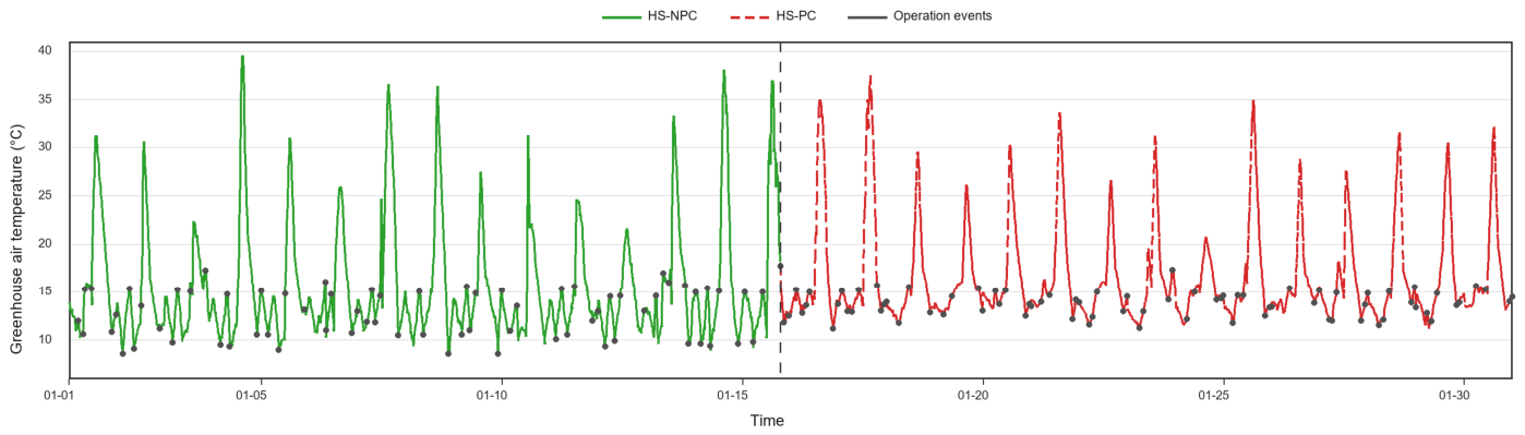
To further evaluate the effect of the prediction-assisted strategy, the system was operated continuously for 30 d. The first 15 d represented the non-predictive control stage (HS-NPC), in which the system was mainly activated according to real-time temperature thresholds. The following 15 d represented the prediction-assisted operation stage (HS-PC), in which the controller adjusted circulating heat release and auxiliary heating in advance based on 12 h, 24 h and 48 h temperature forecasts and low-temperature risk levels. Because the complete 30 d temperature sequence was relatively long, Figure 8 shows only a representative time window around the transition between the two operation stages to illustrate the temperature response and equipment operating states. The complete 30 d sequence of greenhouse air temperature and equipment-operation events is provided in Figure A2 to improve the verifiability of the reported daily averages and operating patterns. The daily scale performance indicators of the two operation stages are shown in Figure 9, and the corresponding stage-level statistical values are summarized in Table 5.
Figure 8.
Night-time temperature variation in the active–passive heat storage and release greenhouse. Note: TG, traditional greenhouse; OT, outdoor temperature; HS-NPC, heat storage and release system without predictive control; HS-PC, heat storage and release system with prediction-assisted operation; DO, circulating heat release on; AH, auxiliary electric heating on; DO+AH, circulating heat release and auxiliary electric heating on; OFF, both circulating heat release and auxiliary electric heating off. The dashed horizontal lines indicate the 10 °C and 13 °C temperature thresholds.
Figure 9.
Operating performance indicators under the two operation stages. Note: (a) Daily minimum indoor temperature; (b) night-time mean temperature; (c) daily mean temperature increase relative to TG; (d) daily duration below 13 °C; (e) daily duration below 10 °C; (f) daily auxiliary electric heating duration. Vertical dashed lines separate the HS-NPC and HS-PC periods, and the horizontal dashed line in panel (c) indicates zero temperature increase relative to TG.
Table 5.
Comparison of operating performance indicators between HS-NPC and HS-PC.
The results in Figure 9 and Table 5 show that, during the consecutive-stage operation test, HS-PC exhibited stronger night-time temperature maintenance and lower low-temperature exposure than HS-NPC. Relative to the HS-NPC stage, the HS-PC stage increased the daily minimum indoor temperature from 9.71 °C to 11.63 °C, corresponding to an increase of 1.92 °C or 19.8%. The night-time mean temperature increased from 12.47 °C to 16.77 °C, corresponding to an increase of 4.29 °C or 34.4%. The daily mean temperature increase relative to TG increased from 4.46 °C to 5.35 °C, corresponding to an increase of 0.89 °C or 20.0%. These results suggest that the improved performance in the HS-PC stage was associated not only with operation intensity, but also with better temporal matching between circulating heat release and night-time cooling based on advance identification of low-temperature risk.
3.2.3. Low-Temperature Exposure and Auxiliary Heating Response
Low-temperature exposure indicators further characterized the stage-based difference between HS-NPC and HS-PC. In the HS-NPC stage, the daily low-temperature warning exposure duration below 13 °C was 10.17 h d−1, whereas it decreased to 4.57 h d−1 in the HS-PC stage, a reduction of 5.59 h d−1 or 55.0%. The daily severe low-temperature exposure duration below 10 °C decreased from 4.02 h d−1 in HS-NPC to 0.07 h d−1 in HS-PC, a reduction of 3.95 h d−1 or 98.2%. This result indicates that, during the continuous low-temperature operation test, severe low-temperature exposure in the HS-PC stage was compressed to a very low level, and the system low-temperature risk shifted more frequently from the severe low-temperature range to the warning range.
The change in auxiliary heating duration suggests that the warmer HS-PC conditions were not associated with a longer electric-heating period. The daily auxiliary heating duration decreased from 7.95 h d−1 in HS-NPC to 4.61 h d−1 in HS-PC, corresponding to a reduction of 3.34 h d−1 or 42.0%. This result suggests that, within the consecutive-stage comparison, HS-PC was associated with less delayed compensation after low temperature had already formed and lower dependence on auxiliary electric heating. In addition, the 30 d heat storage tank water-temperature record is provided in Figure A1 to support the interpretation of stored-heat availability during system operation.
Overall, the active–passive heat storage and release system provided the basic night-time low-temperature buffering capacity, while the HS-PC stage showed better matching between system heat release timing and the low-temperature process under the consecutive-stage comparison. The operating pattern shifted from “responding after the current temperature falls below the threshold” to “intervening before future low-temperature risk forms”, and was accompanied by higher daily minimum temperature, higher night-time mean temperature, shorter low-temperature exposure duration and shorter auxiliary heating duration.
3.3. Energy-Saving Performance
After evaluating the low-temperature buffering capacity of the active–passive heat storage and release system and the stage-based performance of HS-PC, energy consumption was further evaluated on a stage-based equivalent input-energy basis. Because HS-NPC and HS-PC corresponded to two consecutive 15 d operation stages rather than full-month parallel treatments, TG was used as the reference greenhouse for the corresponding period. Therefore, HS-NPC was compared with TG during days 1–15, and HS-PC was compared with TG during days 16–30. The daily equivalent input energy consumption and stage-cumulative equivalent input-energy consumption under the two operation stages are shown in Figure 10.
Figure 10.
Daily and stage-cumulative equivalent input-energy consumption under two consecutive operation stages. Note: TG is the traditional greenhouse and was recorded continuously during the January operation period. HS-NPC represents the heat storage and release greenhouse without predictive control during days 1–15, and HS-PC represents the heat storage and release greenhouse with prediction-assisted operation during days 16–30. Bars indicate daily equivalent input-energy consumption, and lines indicate stage-cumulative equivalent input-energy consumption within each corresponding 15 d stage. The dashed vertical line separates the HS-NPC and HS-PC periods.
During days 1–15, the equivalent input-energy consumption of TG was 2184 kWh, whereas the measured electricity consumption of HS-NPC was 1811 kWh. This indicates that HS-NPC reduced the stage-based equivalent input-energy consumption by 373 kWh relative to TG, corresponding to a stage-based equivalent input-energy reduction rate of 17.1%. During days 16–30, the equivalent input-energy consumption of TG was 2340 kWh, whereas the measured electricity consumption of HS-PC was 1538 kWh. Compared with TG in the same period, HS-PC reduced the stage-based equivalent input-energy consumption by 802 kWh, corresponding to a stage-based equivalent input-energy reduction rate of 34.3%.
The stage-based equivalent input-energy reduction rate increased from 17.1% in the HS-NPC stage to 34.3% in the HS-PC stage, suggesting that HS-PC had more favorable equivalent input-energy performance under the stage-based comparison. Because the two stages were conducted consecutively rather than as fully synchronized parallel treatments, this comparison should be interpreted as a stage-based equivalent input-energy evaluation relative to the TG reference in each period. The results suggest that the energy-saving effect of the active–passive heat storage and release system originated from the partial substitution of conventional heating through daytime heat storage and night-time heat release, whereas the HS-PC stage was associated with less ineffective or delayed energy use because of optimized equipment on–off timing and a shorter auxiliary heating intervention period.
4. Discussion
4.1. Forecasting-Guided System Operation
The results indicate that the value of the LNN model lies not only in improving forecasting accuracy, but also in converting future temperature trajectories into actionable information for heat storage and release control. Winter night-time cooling in solar greenhouses is governed by outdoor low temperature, envelope heat loss, soil thermal inertia and delayed heat release from storage media; therefore, a control strategy based only on the current temperature threshold tends to activate circulation or auxiliary heating after low-temperature stress has already formed. By providing the predicted minimum temperature, the timing of the temperature valley, the cooling trend and the duration of low-temperature exposure, the 12 h, 24 h and 48 h forecasts enabled the system to shift from a passive threshold response to anticipatory regulation. This shift is agronomically relevant because tomato growth, flowering, fruit set and physiological metabolism are sensitive to low night temperature [29,30], and it is also consistent with the thermal inertia of solar greenhouse environments [31]. In the present study, HS-PC increased the daily minimum indoor temperature and night-time mean temperature by 1.92 °C and 4.29 °C, respectively, compared with HS-NPC, while reducing the daily exposure durations below 13 °C and 10 °C by 55.0% and 98.2%, respectively. These results suggest that multi-horizon forecasting may have contributed to system performance by providing a more appropriate activation window for circulating heat release and auxiliary heating, and was associated with better temporal matching between heat supply and the forthcoming cooling process.
4.2. Low-Temperature Buffering Mechanism
The low-temperature buffering effect of the active–passive heat storage and release system was primarily derived from the temporal redistribution of daytime solar heat to night-time heat demand. Compared with TG, which mainly depended on passive heat storage by the wall, soil and thermal insulation structures, HS-NPC added solar heat collection, water-tank storage and floor-pipeline heat release, allowing part of the surplus daytime solar energy to be actively transferred to the night-time low-temperature period. This mechanism is consistent with previous studies showing that solar heat collection combined with soil or storage-media heat release can improve greenhouse thermal stability in cold regions [32,33,34,35]. In this study, the daily mean temperature increase in HS-NPC relative to TG reached 4.46 °C during days 1–15, suggesting the basic buffering capacity of the active–passive system. During days 16–30, HS-PC showed a daily mean temperature increase relative to TG of 5.35 °C and a 98.2% lower daily severe low-temperature exposure duration below 10 °C relative to the HS-NPC stage. Meanwhile, the daily auxiliary heating duration decreased by 42.0%. These results suggest that, under the consecutive-stage comparison, HS-PC was associated with better temporal matching between stored heat release, auxiliary heating and the night-time cooling process, rather than simply extending the auxiliary heating period. This agrees with the broader view that greenhouse energy saving depends on the coordinated balance among crop thermal demand, heat retention, energy input and operating strategy [36].
4.3. Limitations and Future Work
Although the proposed system improved night-time thermal stability and reduced auxiliary electric heating demand, the validation was conducted as a consecutive-stage operation test rather than a fully synchronized parallel experiment. The comparison was supported by the TG reference and by outdoor environmental statistics, including temperature, solar radiation, wind speed and low-temperature degree-hours. Nevertheless, the observed improvements should be interpreted as stage-based operational benefits under the tested winter conditions, rather than as completely weather-independent causal effects.
The current control process was mainly based on predicted air-temperature trajectories, low temperature thresholds and risk levels. Heat storage tank temperature, supply and return water temperatures, circulation flow rate, equipment power, heat load and energy cost were not yet incorporated into a unified optimization framework. In addition, actuator-level constraints such as minimum on/off duration, hysteresis control and tank-temperature-based heat release constraints should be further incorporated in future controller optimization. Future work should extend validation to longer operation periods and multiple winter-weather scenarios, preferably with synchronized parallel experiments or weather-normalized analysis. A multi-objective predictive control strategy that jointly considers low-temperature risk, stored-heat availability and energy consumption should also be developed.
5. Conclusions
This study developed and evaluated a temperature prediction-based active–passive heat storage and release system for night-time low-temperature regulation in winter solar greenhouses. The system integrated environmental monitoring, multi-horizon LNN temperature forecasting, circulating heat storage and release, and auxiliary electric heating control to identify upcoming low-temperature risks and adjust equipment operation in advance. The results showed that the active–passive heat storage and release system provided a basic thermal buffer for maintaining night-time temperature. Under the consecutive-stage comparison, the HS-PC stage showed better matching between the timing of heat release, auxiliary heating and the night-time cooling process. Compared with the non-predictive control stage, HS-PC showed reductions of 55.0% in the daily warning exposure duration below 13 °C, 98.2% in the severe low-temperature exposure duration below 10 °C, and 42.0% in the auxiliary heating duration. These results suggest that the observed stage-based benefit of HS-PC was not achieved simply by extending electric heating time, but was associated with earlier identification of low-temperature risk and optimized on–off timing of circulating heat release and auxiliary heating.
The energy evaluation further showed that the stage-based equivalent input-energy reduction rate was 17.1% for HS-NPC relative to the stage-matched TG reference and increased to 34.3% for HS-PC. This suggests that the active–passive heat storage and release system itself could partially substitute conventional heating demand, while the HS-PC stage showed more favorable stored-heat utilization and equipment-operation performance under the stage-based comparison. Overall, embedding temperature forecasts into greenhouse thermal regulation has the potential to shift system operation from a response based only on current temperature thresholds to an earlier intervention based on future low-temperature risk, providing a feasible approach for low-temperature prevention and energy-saving operation in winter solar greenhouses.
The findings of this study provide a useful reference for low-temperature management in protected horticulture during winter. For other protected crops, greenhouses in cold regions, or production environments with large diurnal temperature differences, the prediction-assisted heat storage and release strategy may also be applicable, but its implementation should be adjusted according to local climate conditions, greenhouse structure, crop low-temperature sensitivity, and heat storage medium characteristics. In particular, low-temperature control thresholds, forecasting input variables, and equipment on–off strategies should not be directly transferred without recalibration. Future work should further verify system performance over longer operation periods, under multiple weather conditions, and preferably through synchronized parallel experiments. Continuous monitoring of thermal-state variables, including tank temperature, supply and return water temperatures, circulation flow rate, and equipment power, should also be strengthened to more accurately evaluate stored-heat availability, the contribution of the control strategy, and the overall operational benefits of the system.
Author Contributions
Conceptualization, J.B. and J.X. (Jianfei Xing); methodology, A.Z., H.G., J.X. (Jianfei Xing), W.L., G.Z. and J.X. (Jiahui Xu); software, A.Z.; validation, A.Z., S.Z. and X.W.; formal analysis, A.Z. and H.G.; investigation, W.L., G.Z. and J.X. (Jiahui Xu); resources, X.W.; data curation, A.Z., S.Z., W.L., G.Z. and J.X. (Jiahui Xu); writing—original draft preparation, A.Z.; writing—review and editing, A.Z., S.Z., H.G., J.B., X.W., J.X. (Jianfei Xing), W.L., G.Z. and J.X. (Jiahui Xu); visualization, A.Z.; supervision, J.B. and J.X. (Jianfei Xing); project administration, H.G., J.B., X.W. and J.X. (Jianfei Xing); funding acquisition, J.B., X.W. and J.X. (Jianfei Xing). All authors have read and agreed to the published version of the manuscript.
Funding
This research was funded by the Bingtuan Innovative Team Project, grant number 2025DB014; the Tianshan Talent Program, grant number 2024TSYCQNTJ005; the Bingtuan Science and Technology Innovation Talent Project, grant number 2024DB031; the 14th Five-Year National Key R&D Program of China, grant number 2023YFD2000600; the Bingtuan Key-Area Science and Technology Research Project, grant number 2023AB005-01; the Division-City Science and Technology Research Plan Project, grant number TDZKSS202440; the University-level Research Project, grant number TDGRI2024066; and the University-level Research Project, grant number TDBSCX202521.
Institutional Review Board Statement
Not applicable.
Data Availability Statement
The data presented in this study are available from the corresponding authors upon reasonable request.
Conflicts of Interest
The authors declare no conflicts of interest. The funders had no role in the design of the study; in the collection, analyses, or interpretation of data; in the writing of the manuscript; or in the decision to publish the results.
Abbreviations
The following abbreviations are used in this manuscript:
| TG | Traditional greenhouse |
| OT | Outdoor temperature |
| HS-NPC | Heat storage and release system without predictive control |
| HS-PC | Heat storage and release system with prediction-assisted operation |
| DO | Circulating heat release on |
| AH | Auxiliary electric heating on |
| DO+AH | Circulating heat release and auxiliary electric heating on |
| OFF | Circulating heat release and auxiliary electric heating off |
| LNN | Liquid neural network |
| GRU | Gated recurrent unit |
| XGBoost | Extreme Gradient Boosting |
| IoT | Internet of Things |
| RMSE | Root mean square error |
| MAE | Mean absolute error |
| PAR | Photosynthetically active radiation |
| PVC | Polyvinyl chloride |
| PE-RT | Polyethylene of raised temperature resistance |
| ODE | Ordinary differential equation |
| LHV | Lower heating value |
| NRMSE | Normalized root mean square error |
Appendix A
Table A1.
One-factor-at-a-time sensitivity analysis of key LNN hyperparameters.
Table A2.
Control-oriented forecasting metrics of different models under different prediction horizons.
Table A3.
Main decision rules and actuator states used in the prediction-assisted operation strategy.
Appendix B
Figure A1.
Evolution of heat storage tank water temperature during the 30 d operation period. Note: The heat storage tank water temperature was recorded from 1 January to 30 January 2026. The vertical dashed line indicates the transition from HS-NPC to HS-PC. The record is provided as supplementary evidence of stored-heat availability during system operation.
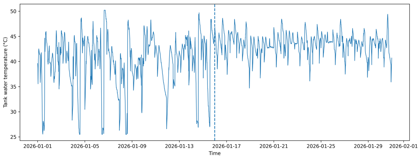
Figure A2.
Thirty-day greenhouse air temperature and equipment-operation events during the operation period. Note: The green solid line represents the HS-NPC stage from 1 January to 15 January 2026, and the red dashed line represents the HS-PC stage from 16 January to 30 January 2026. Gray markers indicate recorded equipment-operation events during system operation.
References
- Shamshiri, R.R.; Jones, J.W.; Thorp, K.R.; Ahmad, D.; Che Man, H.; Taheri, S. Review of optimum temperature, humidity, and vapour pressure deficit for microclimate evaluation and control in greenhouse cultivation of tomato: A review. Int. Agrophys. 2018, 32, 287–302. [Google Scholar] [CrossRef] [Scilit]
- Zhang, M.; Yan, T.; Wang, W.; Jia, X.; Wang, J.; Klemeš, J.J. Energy-saving design and control strategy towards modern sustainable greenhouse: A review. Renew. Sustain. Energy Rev. 2022, 164, 112602. [Google Scholar] [CrossRef] [Scilit]
- Li, N.; Xu, W.; Zhang, Y.; Ma, W.; Ren, Y. Energy saving technologies and practices in facility agriculture in cold regions. Agronomy 2025, 15, 204. [Google Scholar] [CrossRef] [Scilit]
- Zhang, X.; Xie, J.; Ma, N.; Chang, Y.; Zhang, J.; Li, J. Energy simulation-driven life-cycle costing of Gobi solar greenhouses: Stakeholder-focused analysis for tomato production. Agriculture 2025, 15, 2053. [Google Scholar] [CrossRef] [Scilit]
- Choab, N.; Allouhi, A.; El Maakoul, A.; Kousksou, T.; Saadeddine, S.; Jamil, A. Review on greenhouse microclimate and application: Design parameters, thermal modeling and simulation, climate controlling technologies. Sol. Energy 2019, 191, 109–137. [Google Scholar] [CrossRef] [Scilit]
- Lu, W.; Zhang, Y.; Fang, H.; Ke, X.; Yang, Q. Modelling and experimental verification of the thermal performance of an active solar heat storage-release system in a Chinese solar greenhouse. Biosyst. Eng. 2017, 160, 12–24. [Google Scholar] [CrossRef] [Scilit]
- Xu, W.; Guo, H.; Ma, C. An active solar water wall for passive solar greenhouse heating. Appl. Energy 2022, 308, 118270. [Google Scholar] [CrossRef] [Scilit]
- Wang, L.; Li, Y.; Sun, Z.; Meng, S.; Li, T.; Liu, X. Utilization of surplus air thermal energy by a water cycle system in a Chinese-type solar greenhouse. Agronomy 2024, 14, 270. [Google Scholar] [CrossRef] [Scilit]
- Xia, T.; Li, Y.; Wu, X.; Fan, Z.; Shi, W.; Liu, X.; Li, T. Performance of a new active solar heat storage–release system for Chinese assembled solar greenhouses used in high latitudes and cold regions. Energy Rep. 2022, 8, 784–797. [Google Scholar] [CrossRef] [Scilit]
- Luo, Q.L.; Cheng, R.F.; Zhang, Y.; Fang, H.; Li, D.; Zhang, J.F.; Song, G.X. Optimization of active heat storage and release system in solar greenhouse. Trans. Chin. Soc. Agric. Eng. 2020, 36, 234–241. (In Chinese) [Google Scholar] [CrossRef]
- Guan, Y.; Chen, Y.; Zhou, L.; Wei, Z.; Hu, W.; Yang, Y. The thermal properties of an active–passive heat storage wall system incorporating phase change materials in a Chinese solar greenhouse. Sustainability 2024, 16, 2624. [Google Scholar] [CrossRef] [Scilit]
- Shukla, A.; Sharma, A.; Kant, K. Solar greenhouse with thermal energy storage: A review. Curr. Sustain. Renew. Energy Rep. 2016, 3, 58–66. [Google Scholar] [CrossRef] [Scilit]
- Nishad, S.; Krupa, I. Phase change materials for thermal energy storage applications in greenhouses: A review. Sustain. Energy Technol. Assess. 2022, 52, 102241. [Google Scholar] [CrossRef] [Scilit]
- Zhang, S.; Guo, Y.; Zhao, H.; Wang, Y.; Chow, D.; Fang, Y. Methodologies of control strategies for improving energy efficiency in agricultural greenhouses. J. Clean. Prod. 2020, 274, 122695. [Google Scholar] [CrossRef] [Scilit]
- Guo, Y.; Zhao, H.; Zhang, S.; Wang, Y.; Chow, D. Modeling and optimization of environment in agricultural greenhouses for improving cleaner and sustainable crop production. J. Clean. Prod. 2021, 285, 124843. [Google Scholar] [CrossRef] [Scilit]
- Vanthoor, B.H.E.; Stanghellini, C.; van Henten, E.J.; de Visser, P.H.B. A methodology for model-based greenhouse design: Part 1, a greenhouse climate model for a broad range of designs and climates. Biosyst. Eng. 2011, 110, 363–377. [Google Scholar] [CrossRef] [Scilit]
- Katzin, D.; van Henten, E.J.; van Mourik, S. Process-based greenhouse climate models: Genealogy, current status, and future directions. Agric. Syst. 2022, 198, 103388. [Google Scholar] [CrossRef] [Scilit]
- Ferreira, P.M.; Faria, E.A.; Ruano, A.E. Neural network models in greenhouse air temperature prediction. Neurocomputing 2002, 43, 51–75. [Google Scholar] [CrossRef] [Scilit]
- Francik, S.; Kurpaska, S. The use of artificial neural networks for forecasting of air temperature inside a heated foil tunnel. Sensors 2020, 20, 652. [Google Scholar] [CrossRef] [Scilit] [PubMed]
- Ma, D.; Carpenter, N.; Maki, H.; Rehman, T.U.; Tuinstra, M.R.; Jin, J. Greenhouse environment modeling and simulation for microclimate control. Comput. Electron. Agric. 2019, 162, 134–142. [Google Scholar] [CrossRef] [Scilit]
- Shi, D.; Yuan, P.; Liang, L.; Gao, L.; Li, M.; Diao, M. Integration of deep learning and sparrow search algorithms to optimize greenhouse microclimate prediction for seedling environment suitability. Agronomy 2024, 14, 254. [Google Scholar] [CrossRef] [Scilit]
- Ding, Y.; Wang, L.; Li, Y.; Li, D. Model predictive control and its application in agriculture: A review. Comput. Electron. Agric. 2018, 151, 104–117. [Google Scholar] [CrossRef] [Scilit]
- Blasco, X.; Martínez, M.; Herrero, J.M.; Ramos, C.; Sanchis, J. Model-based predictive control of greenhouse climate for reducing energy and water consumption. Comput. Electron. Agric. 2007, 55, 49–70. [Google Scholar] [CrossRef] [Scilit]
- Lin, D.; Zhang, L.; Xia, X. Model predictive control of a Venlo-type greenhouse system considering electrical energy, water and carbon dioxide consumption. Appl. Energy 2021, 298, 117163. [Google Scholar] [CrossRef] [Scilit]
- Mahmood, F.; Govindan, R.; Bermak, A.; Yang, D.; Khadra, C.; Al-Ansari, T. Energy utilization assessment of a semi-closed greenhouse using data-driven model predictive control. J. Clean. Prod. 2021, 324, 129172. [Google Scholar] [CrossRef] [Scilit]
- Mahmood, F.; Govindan, R.; Bermak, A.; Yang, D.; Al-Ansari, T. Data-driven robust model predictive control for greenhouse temperature control and energy utilisation assessment. Appl. Energy 2023, 343, 121190. [Google Scholar] [CrossRef] [Scilit]
- Hasani, R.; Lechner, M.; Amini, A.; Rus, D.; Grosu, R. Liquid time-constant networks. In Proceedings of the AAAI Conference on Artificial Intelligence, Virtual Event, 2–9 February 2021; Volume 35, pp. 7657–7666. [Google Scholar] [CrossRef] [Scilit]
- Chen, T.; Guestrin, C. XGBoost: A scalable tree boosting system. In Proceedings of the 22nd ACM SIGKDD International Conference on Knowledge Discovery and Data Mining, San Francisco, CA, USA, 13–17 August 2016; Association for Computing Machinery: New York, NY, USA, 2016; pp. 785–794. [Google Scholar] [CrossRef] [Scilit]
- Yang, E.Y.; Rajametov, S.N.; Cho, M.C.; Jeong, H.B.; Chae, W.B. Factors affecting tolerance to low night temperature differ by fruit types in tomato. Agriculture 2021, 11, 681. [Google Scholar] [CrossRef] [Scilit]
- Rajametov, S.N.; Lee, K.; Jeong, H.B.; Cho, M.C.; Nam, C.W.; Yang, E.Y. Physiological traits of thirty-five tomato accessions in response to low temperature. Agriculture 2021, 11, 792. [Google Scholar] [CrossRef] [Scilit]
- Zhang, Y.; Xu, L.; Zhu, X.; He, B.; Chen, Y. Thermal environment model construction of Chinese solar greenhouse based on temperature-wave interaction theory. Energy Build. 2023, 279, 112648. [Google Scholar] [CrossRef] [Scilit]
- Zhao, J.; Chen, F.; Wang, Y.; Wang, K.; Zhai, X.; Zhang, D. Experimental study on effect of an active solar heating soil heat storage system on the thermal environment in Gobi solar greenhouses. Energy Build. 2024, 325, 115055. [Google Scholar] [CrossRef] [Scilit]
- Yu, T.; Wang, D.; Zhao, X.; Liu, J.; Kim, M.K. Experimental and numerical study of an active solar heating system with soil heat storage for greenhouses in cold climate zones. Buildings 2022, 12, 405. [Google Scholar] [CrossRef] [Scilit]
- Chen, W.; Zhou, G. Experimental investigation on heating performance of long- and short-term PCM storage in Chinese solar greenhouse. J. Energy Storage 2024, 99, 113466. [Google Scholar] [CrossRef] [Scilit]
- Zhang, L.; Xu, P.; Mao, J.; Tang, X.; Li, Z.; Shi, J. A low-cost seasonal solar soil heat storage system for greenhouse heating: Design and pilot study. Appl. Energy 2015, 156, 213–222. [Google Scholar] [CrossRef] [Scilit]
- Ahamed, M.S.; Guo, H.; Tanino, K. Energy-saving techniques for reducing the heating cost of conventional greenhouses. Biosyst. Eng. 2019, 178, 9–33. [Google Scholar] [CrossRef] [Scilit]
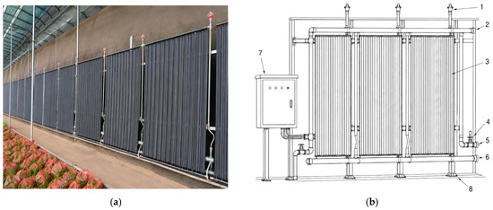
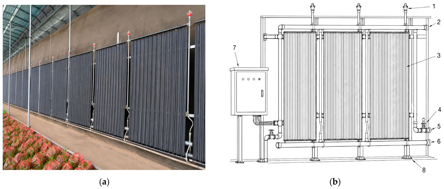
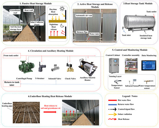
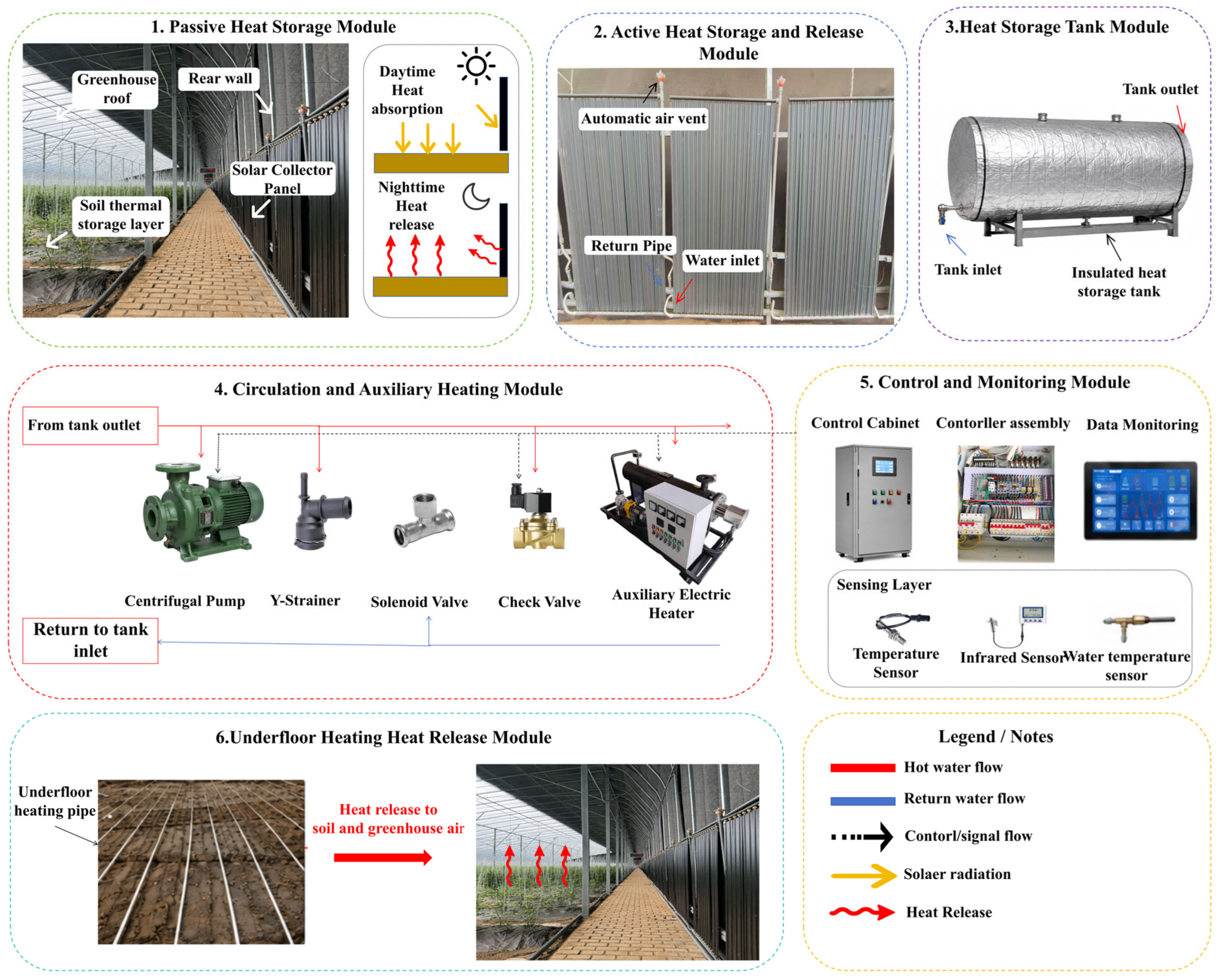
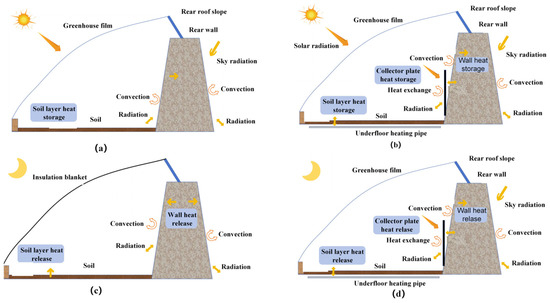
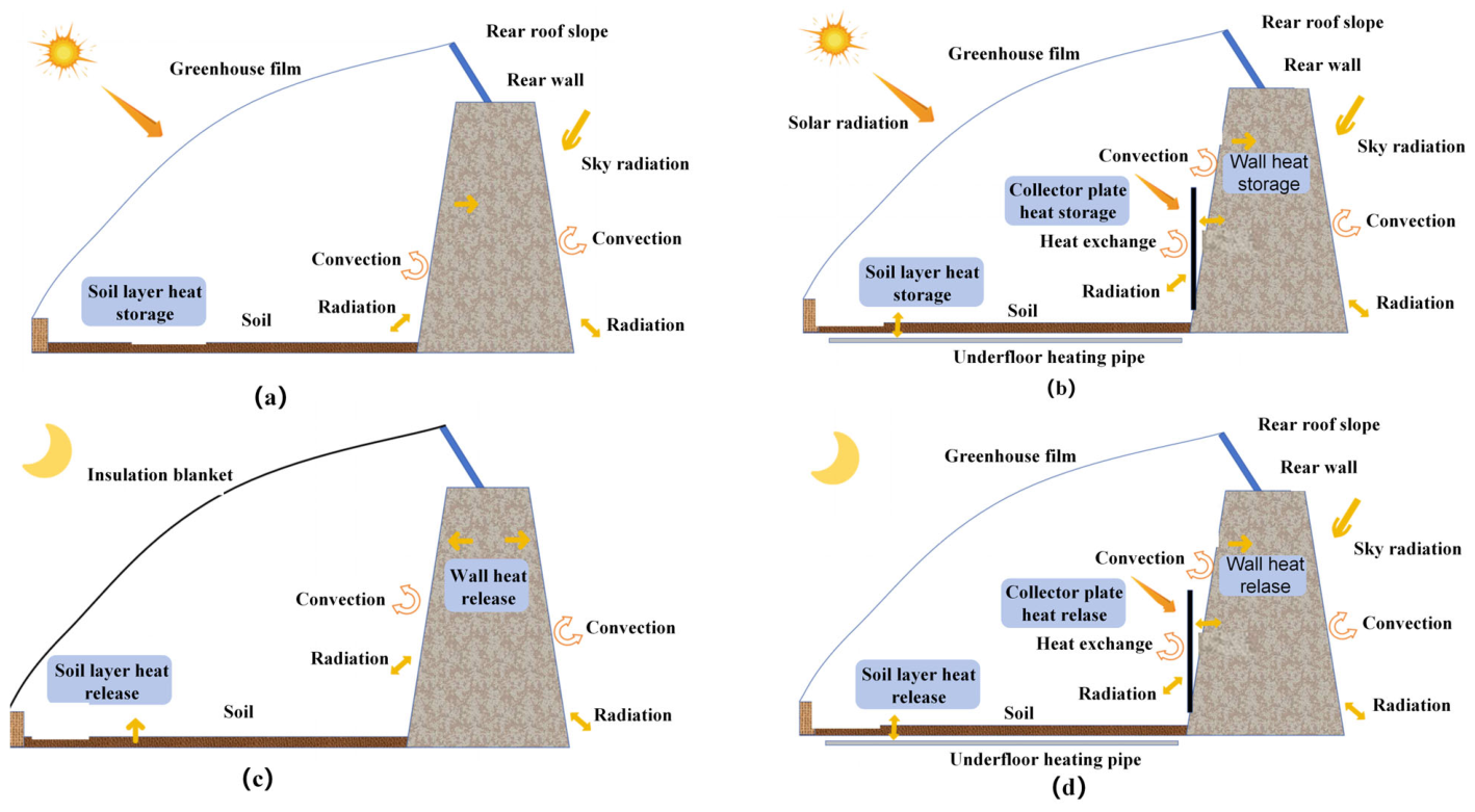
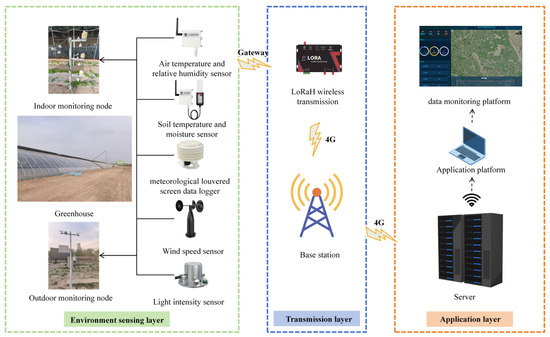
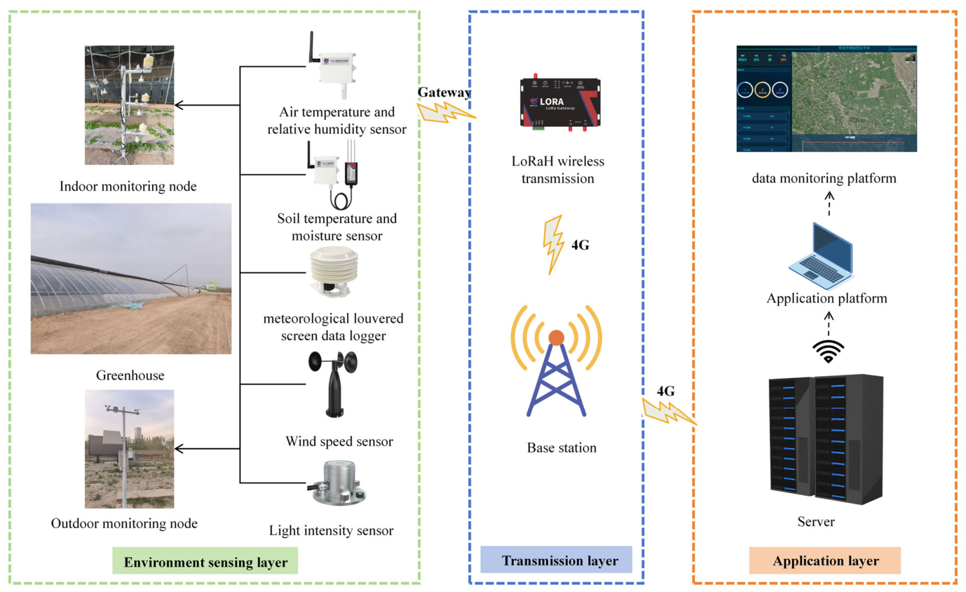
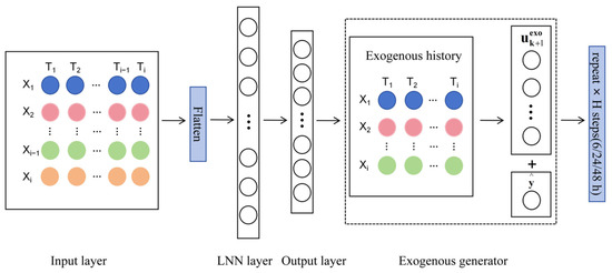
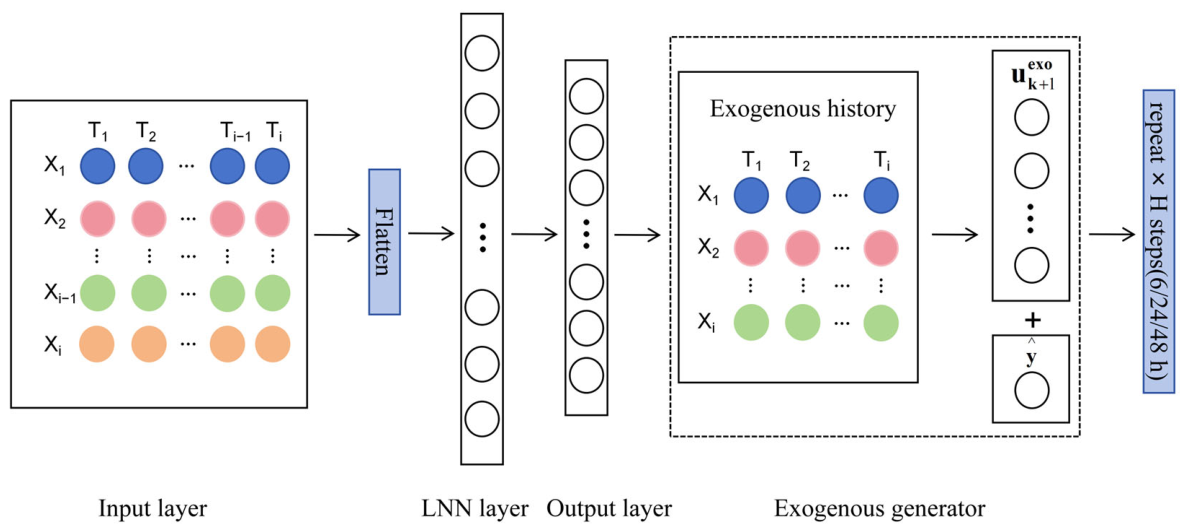
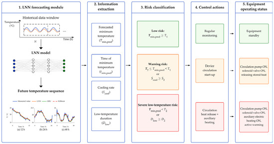
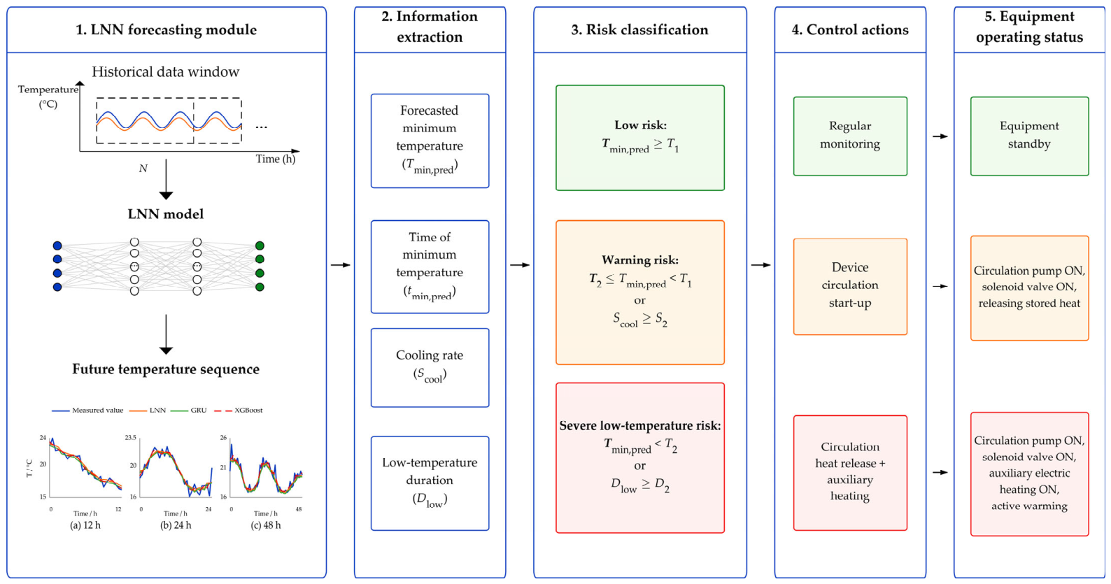
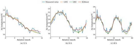
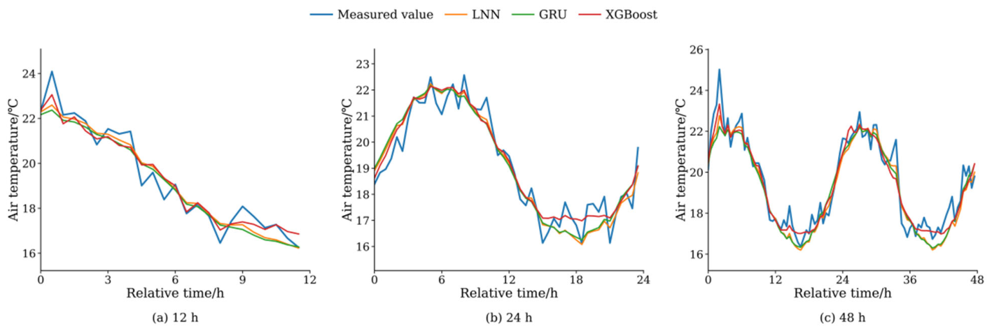
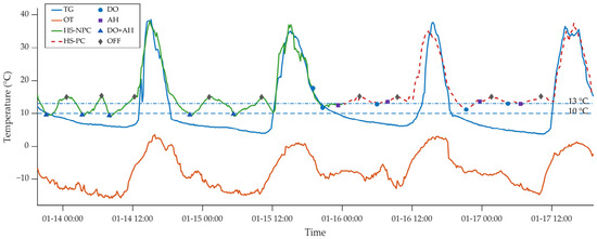
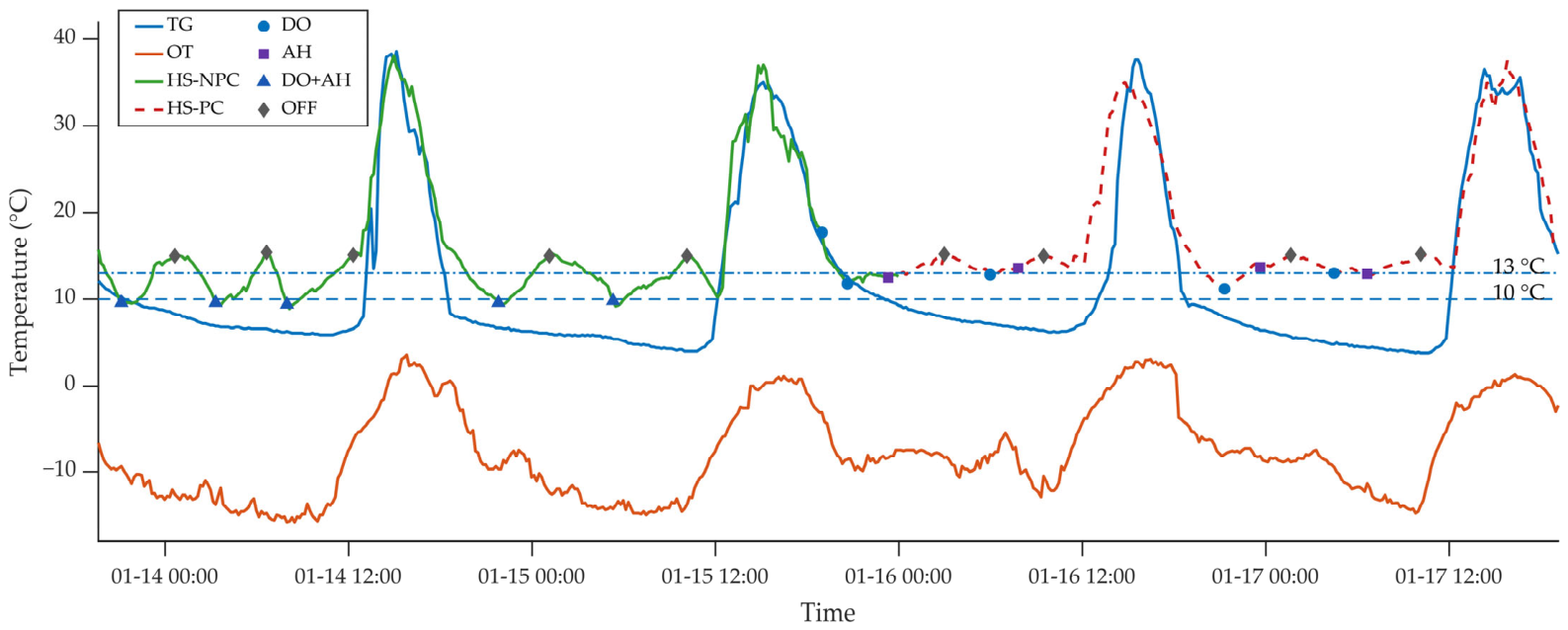
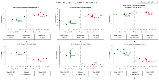
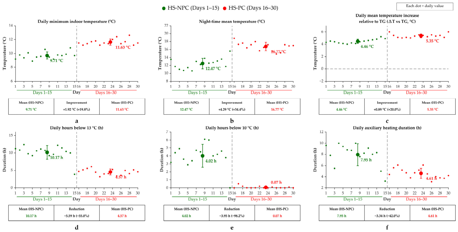
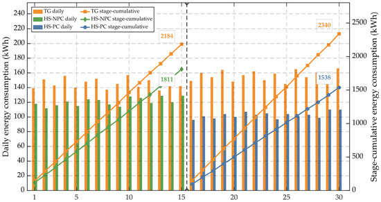
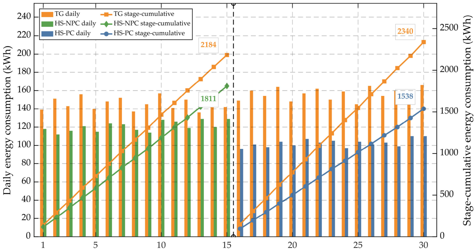

Disclaimer/Publisher’s Note: The statements, opinions and data contained in all publications are solely those of the individual author(s) and contributor(s) and not of MDPI and/or the editor(s). MDPI and/or the editor(s) disclaim responsibility for any injury to people or property resulting from any ideas, methods, instructions or products referred to in the content. |
© 2026 by the authors. Licensee MDPI, Basel, Switzerland. This article is an open access article distributed under the terms and conditions of the Creative Commons Attribution (CC BY) license.