1. Introduction
Energy system optimization aims to utilize different energy sources in the most efficient manner under technical, economic, and environmental constraints, encompassing various improvement processes. Higher energy demand, the large-scale integration of renewables into energy systems, and sustainability requirements have turned the optimal planning and operation of energy systems into a necessity. In this context, the effective management of hybrid energy systems that incorporate multiple energy sources plays a critical role in ensuring energy supply security and minimizing costs.
The optimization of hybrid energy systems is a complex problem that requires the joint consideration of energy generation, storage, and consumption components. In such systems, the variable nature of energy resources, uncertainties in load demand, and system constraints further complicate the solution process.
In the literature, various classical methods have been widely employed to address these problems, including Linear Programming (LP), Nonlinear Programming, Quadratic Programming, decision trees, simulation-based models, and discrete-event simulations. Although such methods yield successful outcomes under certain assumptions, their computational cost and limited solution flexibility can become drawbacks when the problem is high-dimensional and nonlinear.
More recently, advances in data-driven approaches together with the growth in computational capacity have brought deep learning-based methods to the forefront of energy system optimization. Their ability to model complex, nonlinear relationships has turned deep learning techniques into effective instruments for supporting decision-making in hybrid energy systems. Compared to classical optimization methods, these approaches have the potential to generate solutions more rapidly and to represent system behaviors with greater accuracy.
The main objective of this study is to propose a deep learning–based surrogate approach that can approximate the optimal sizing of hybrid energy systems, substantially reducing the computational effort required compared with repeatedly running the underlying optimization. Through the developed methodology, the study aims to improve resource utilization in hybrid energy systems, enhance system performance, and achieve more economically efficient solutions. It is anticipated that the results obtained will enrich the current literature on hybrid energy system planning and operation and serve as a reference for subsequent studies.
Literature Review
The literature review indicates that classical optimization algorithms are widely employed in energy forecasting and optimization problems, whereas deep learning–based approaches have been addressed in a relatively limited number of studies. Especially over the past few years, the capacity of deep learning models to represent complex, nonlinear relationships has been found to enhance renewable energy forecasting performance. Accordingly, the scope and objectives of the present study have been defined in line with these developments.
In studies focusing on the prediction of power generation from renewable energy sources, the effectiveness of deep learning and hybrid models is frequently emphasized. Zheng et al. [
1] proposed a hybrid framework to forecast power generation from multiple renewable energy sources and utilized convolutional neural networks (CNNs) to extract local correlations among different energy sources.
In research concentrating on solar energy systems, time series–based forecasting approaches have become prominent. Kıymaz [
2] employed long short-term memory (LSTM) networks to perform forward-looking generation forecasts using production data from solar power plants at different temporal resolutions and compared the results with those obtained using the SARIMA model. The findings demonstrated that the LSTM model outperformed statistical methods in terms of most performance metrics.
Studies incorporating meteorological data have reported improved forecasting accuracy through the use of artificial neural networks and dynamic models. Orman and Köse [
3] predicted the electricity generation of a solar power plant using an NARX-based artificial neural network model driven by hourly meteorological parameters. Similarly, Kara [
4] showed that an LSTM-based model exhibited superior performance in solar irradiance forecasting compared to various machine learning algorithms.
Machine learning and deep learning methods are also widely applied in wind energy forecasting studies. Yazıcı [
5] developed both static and dynamic hybrid models for short-term wind power forecasting; Bayesian optimization was employed for hyperparameter tuning in the static models, while LSTM networks were utilized in the dynamic model. In the field of electrical load forecasting, Kamber et al. [
6] conducted short-term demand forecasting using LSTM-based artificial neural networks and compared the results with those of the ARIMA model.
Moreover, at the national scale, deep learning approaches have been used for installed capacity forecasting. Özdemir et al. [
7] presented a comparative analysis using artificial neural networks (ANN) and bidirectional LSTM (BLSTM) models to forecast Turkey’s installed solar power capacity.
In the international literature, CNNs, LSTMs, and hybrid combinations of these models are frequently preferred for short-term power forecasting problems in photovoltaic systems [
8,
9,
10,
11,
12,
13,
14,
15,
16,
17]. These studies demonstrate that deep learning–based models achieve high accuracy in both deterministic and probabilistic forecasting tasks. Furthermore, comprehensive review studies on wind and solar energy systems [
18,
19] have highlighted that deep learning models offer a more flexible and powerful structure compared to traditional methods. Recent studies have further expanded these research directions. Metaheuristic-based optimization techniques combined with hybrid CNN–LSTM architectures have been developed to improve short-term photovoltaic and wind power forecasting in smart grid applications [
20,
21]. In addition, comparative studies have evaluated the performance of time-series, deep learning, and hybrid forecasting approaches for estimating electricity generation from multiple energy sources at the national level [
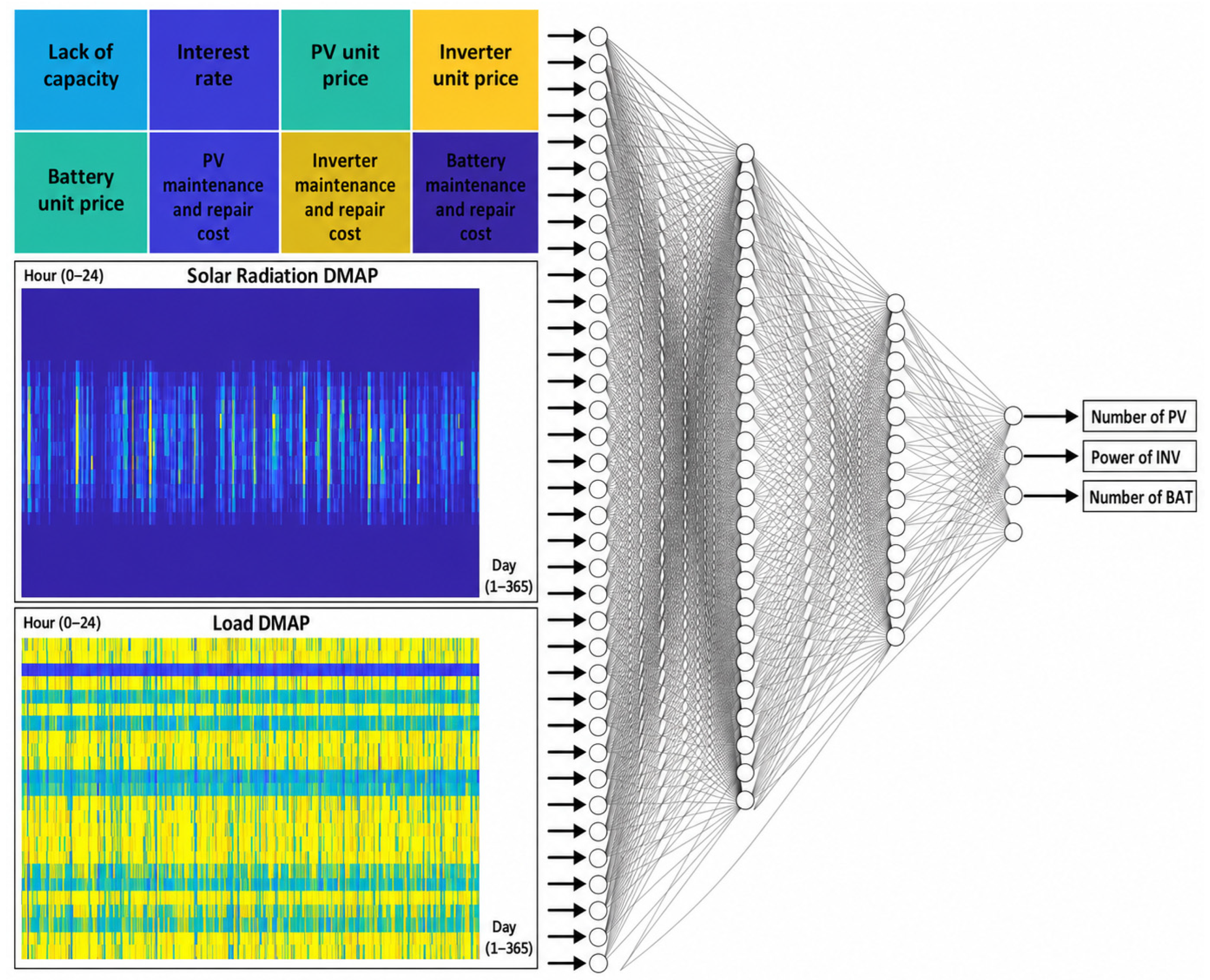
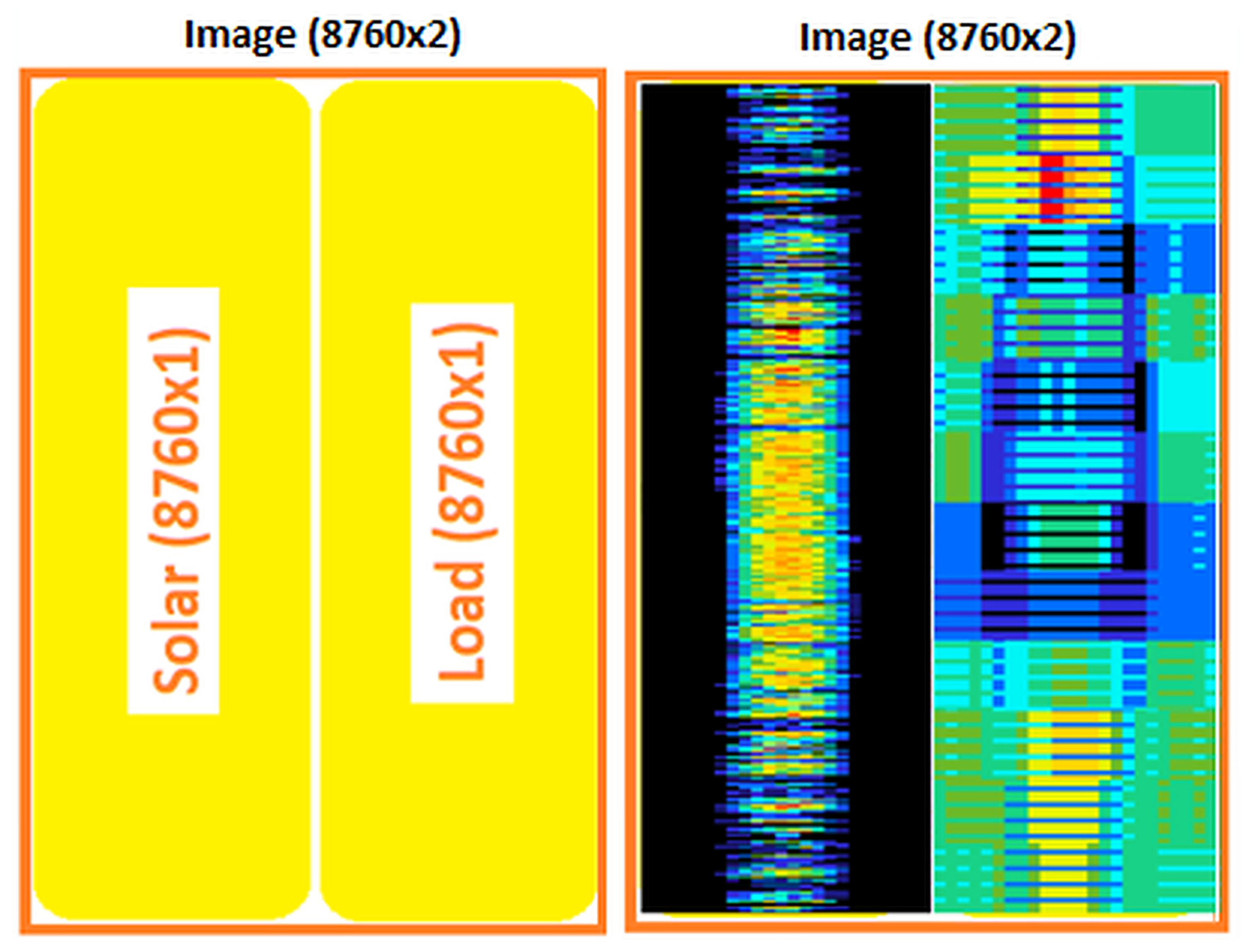
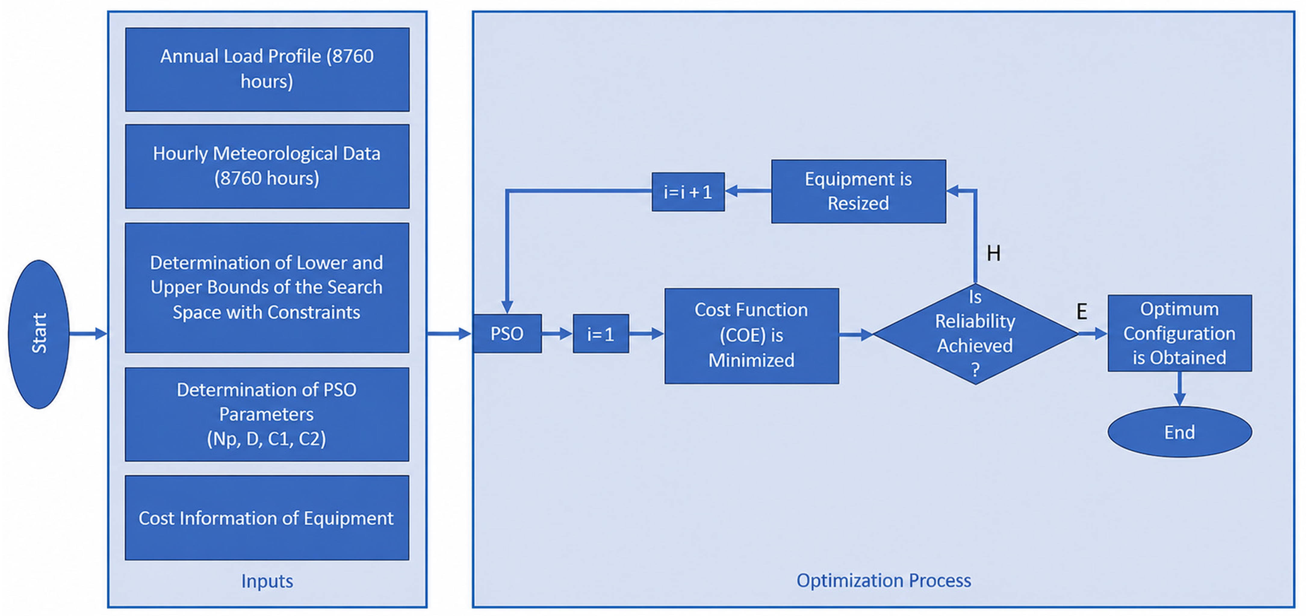
22]. Overall, although a substantial number of studies in the literature address renewable energy generation forecasting, there remains a limited number of works that integrate deep learning–based approaches with optimization processes. Despite these advances, the primary focus of existing studies has been on applying deep learning to forecast renewable energy generation or electricity demand rather than to optimize the sizing of hybrid PV–wind–battery systems. In most cases, this sizing problem is still addressed using iterative metaheuristic algorithms such as Particle Swarm Optimization (PSO), which require considerable computational effort. Accordingly, the main challenge targeted in this study is reducing the computational cost associated with repeatedly performing metaheuristic-based sizing for multiple candidate locations or operating scenarios. To address this challenge, the proposed approach reformulates the component sizing problem as an image-based regression task. Annual hourly profiles of solar irradiance, electrical load, and the corresponding economic parameters are transformed into multi-channel Data Map (DMAP) images, which are used as inputs to convolutional neural networks (CNNs). This representation enables the CNNs to capture local spatial patterns embedded in the encoded time-series data, an advantage that conventional tabular regression models are generally unable to exploit.
In line with this, the principal contributions of this study can be summarized as follows: (i) a DMAP-based representation that transforms annual time-series and economic data into image formats suitable for CNN-based learning; (ii) a supervised dataset constructed by pairing PSO-derived optimal sizing solutions with their corresponding DMAP images; and (iii) a comprehensive evaluation of eight CNN architectures as computationally efficient surrogate models for PSO-based sizing of hybrid renewable energy systems.
3. Results
3.1. MobileNet Results
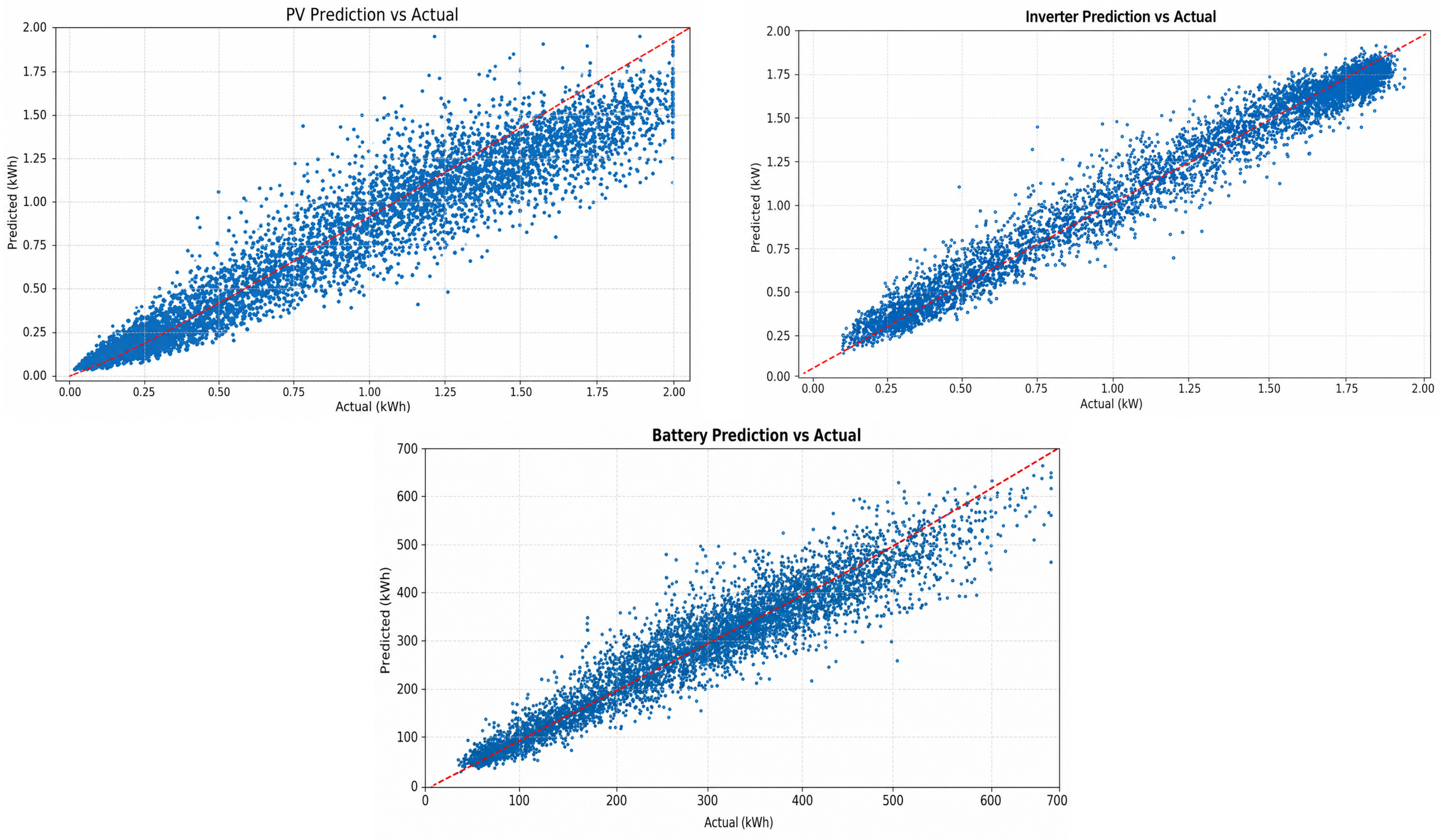
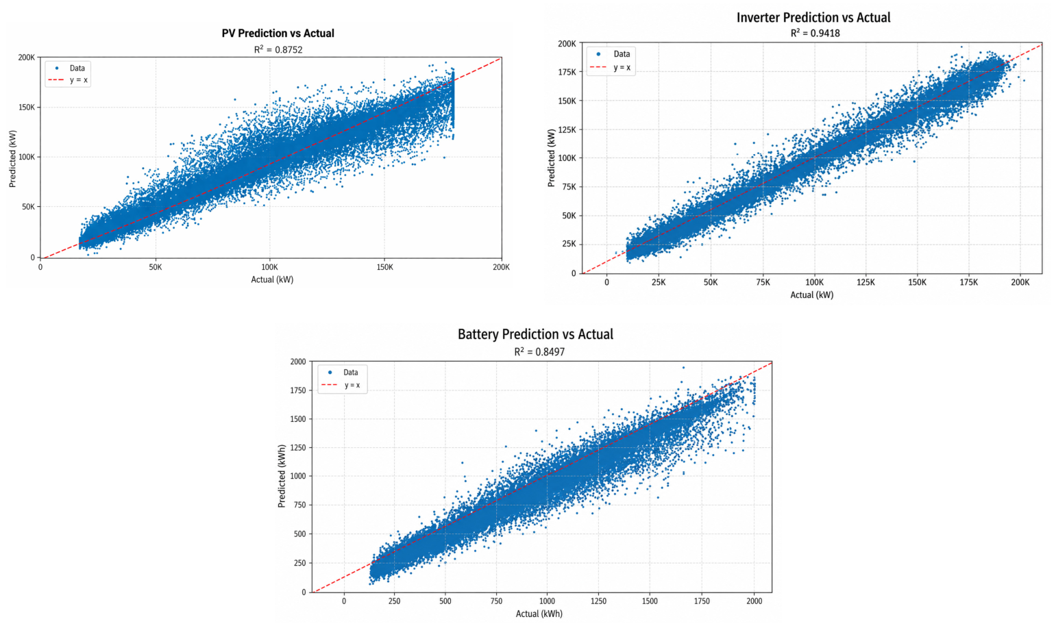
To evaluate the predictive performance of the model on the output variables, prediction–actual comparison plots were generated for the number of photovoltaic (PV) panels, inverter capacity, and battery units. In these plots, the horizontal axis represents the actual (optimal) values, while the vertical axis denotes the values predicted by the model. The red dashed line corresponds to the ideal prediction line (y = x) (
Figure 4).
When the PV panel prediction graph is examined, it is observed that the model generally produces successful predictions. Although the majority of the data points are located close to the ideal line, deviations increase particularly at higher PV values. This indicates that the model operates with reduced sensitivity under high-generation scenarios. The average percentage accuracy obtained for the PV output is 82.55%, demonstrating that the model provides an acceptable level of accuracy for practical applications. However, to further improve this performance, the number of training samples with high PV values could be increased, or the model could be weighted more heavily toward higher-value ranges (
Figure 5).
The prediction–actual comparison graph generated for inverter capacity reveals that the model performs with higher accuracy for this parameter. The data points are more tightly clustered around the ideal line, with relatively small deviations. This suggests that the model produces more stable and reliable outputs when predicting inverter capacity. A more balanced data distribution and the more direct relationship between inverter capacity and the input parameters may have contributed to this performance. The average percentage accuracy of the model in predicting inverter capacity is calculated as 91.32%. This high accuracy indicates that the model provides reliable results for a critical component such as inverter sizing. One possible reason for this success is the more linear and predictable relationship between inverter capacity and the input variables.
In the case of battery predictions, the model attains an accuracy of 85.3%, higher than the PV result yet lower than the inverter capacity result.
Overall, the model generates successful predictions. The per-output error, success, and R
2 values obtained for this model are reported in
Table 3.
Such results indicate that the model estimates the optimal system sizes correctly in the majority of cases, reaching an accuracy adequate for practical use. Nevertheless, in order to further enhance the model—particularly for high-generation scenarios in PV panel predictions—advanced learning techniques, increased sample diversity, and error-weighting strategies can be considered.
3.2. ResNet Results
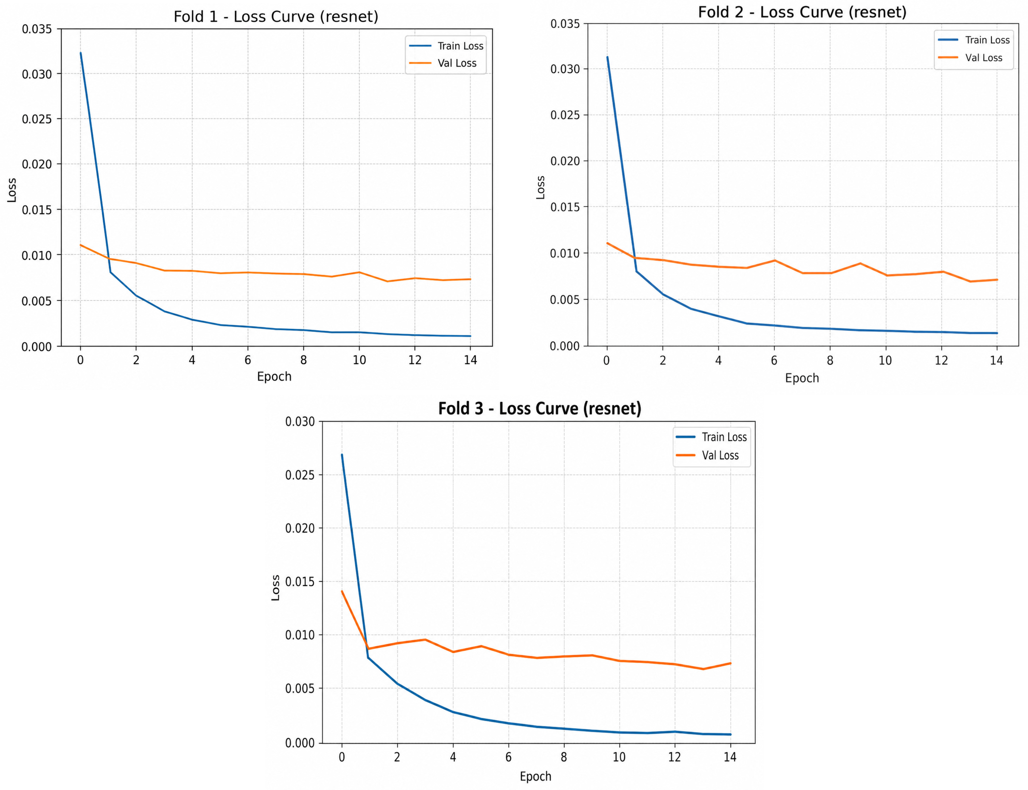
When the loss functions corresponding to the cross-validation layers are examined, it is observed that the initially high loss values gradually decrease. This demonstrates that the network successfully learns the data through three-layer cross-validation (
Figure 6).
When the performance results are examined, the data points are largely clustered around the y = x line. This indicates that the model generally produces predictions that are very close to the actual values. An R
2 value of 0.9285 is considerably high, meaning that the model explains 92.85% of the variance, and thus demonstrates very strong predictive performance (
Figure 7).
Regarding the inverter prediction results, the model performs exceptionally well in estimating inverter capacity. The predicted values are very close to the actual values, and the predictions are highly stable, with minimal error particularly in the mid-range values. Although a slight deviation tendency is observed at very high inverter capacities, this deviation remains within acceptable tolerance limits. The R2 value of 0.9834 is remarkably high, indicating that the model explains 98.34% of the data variance.
For the battery prediction results, an R2 value of 0.9457 is also notably high; however, it is slightly lower than those obtained for PV (0.964) and inverter (0.9834) predictions. The model provides a strong estimation of battery capacity, although deviations are somewhat more pronounced compared to the other outputs.
Overall, the model generates successful predictions. The per-output error, success, and R
2 values obtained for this model are reported in
Table 3.
As observed, the ResNet architecture yields better results compared to the MobileNet network.
3.3. RegNet Results
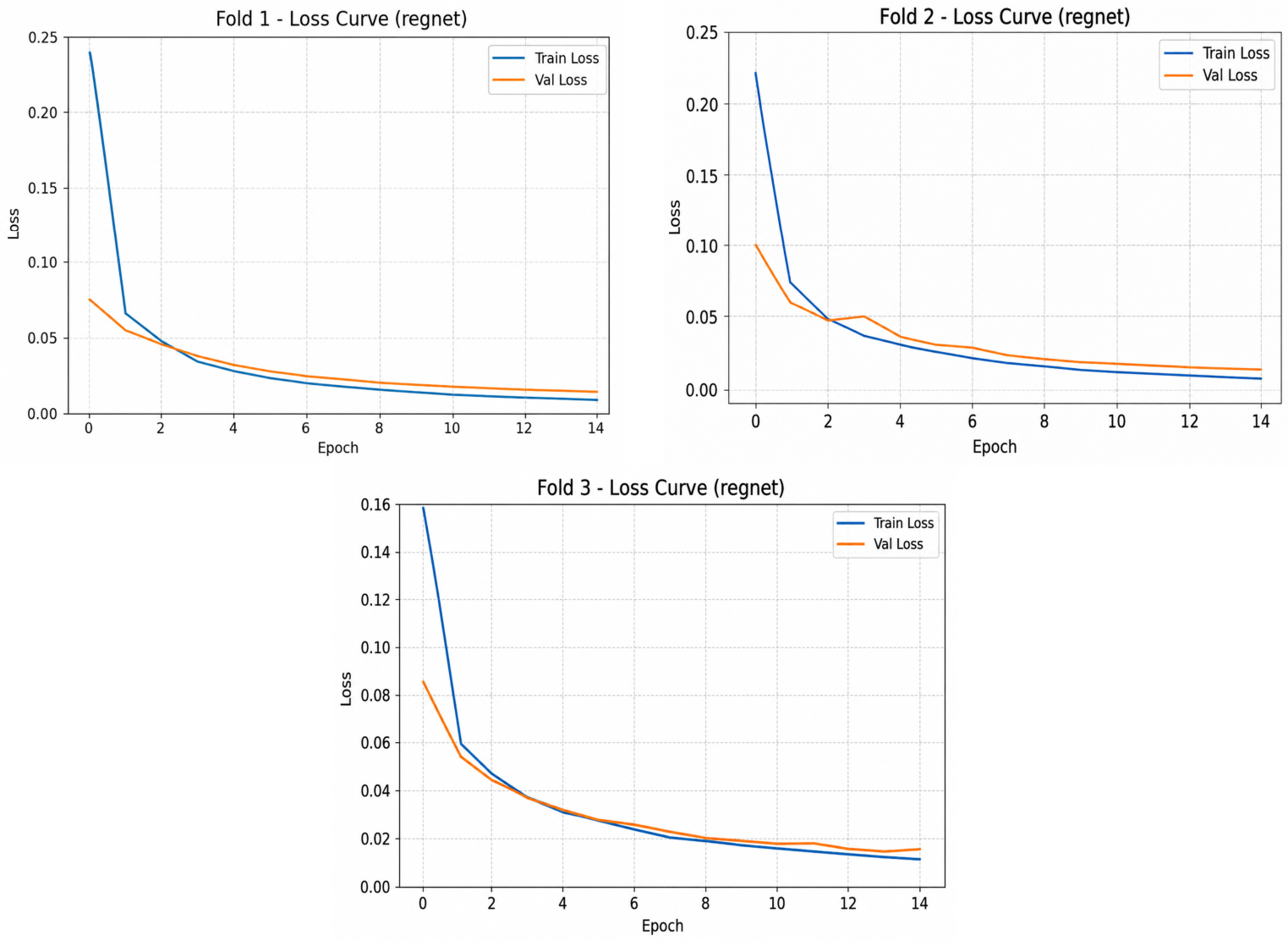
When the loss curves of the RegNet model for the training and validation datasets are examined, a clear decreasing trend is observed in both curves as the number of epochs increases. This indicates that the model effectively learns from the training data while also exhibiting strong generalization performance on the validation data. The close alignment of the training and validation loss curves suggests that overfitting does not occur. Moreover, the steady decrease and consistently low values of the validation loss further support the model’s ability to reliably predict the target outputs (
Figure 8).
This loss curve demonstrates that the RegNet architecture achieves a stable and effective learning process. Overall, it indicates that the RegNet model is trained in a stable and efficient manner with strong generalization capability. No overfitting is observed, and the model adapts well to the validation data, which is consistent with the reported average accuracy of 87.97%.
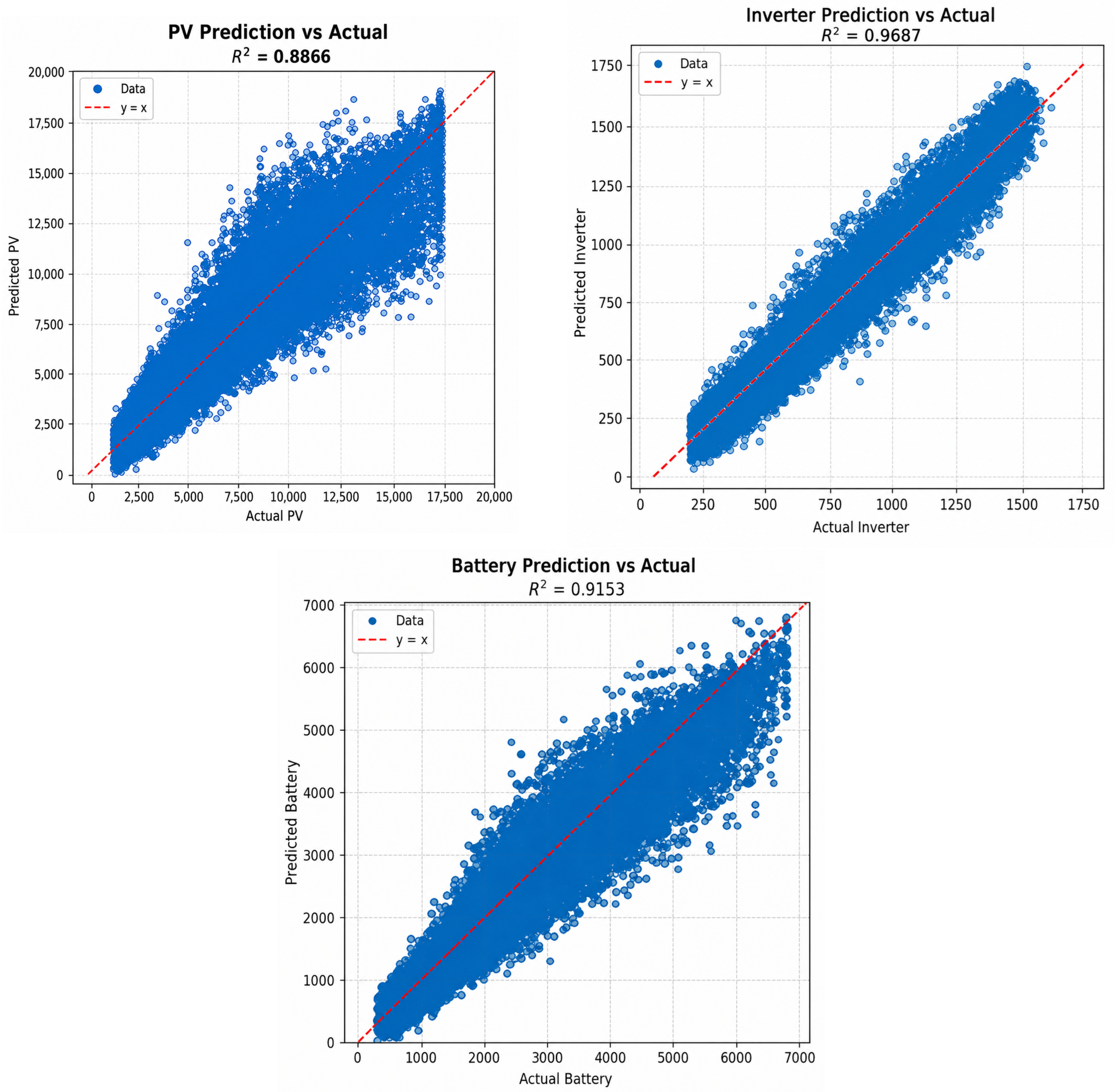
The PV panel number prediction results obtained using the RegNet architecture demonstrate high accuracy with an R
2 value of 0.8866. The majority of the predicted values are clustered around the ideal regression line, indicating that the model exhibits a strong overall generalization capability. Predictions are particularly accurate for low and medium PV panel counts. However, a slight underestimation tendency is observed at higher PV values. This behavior may stem from an imbalanced data distribution or from the model’s limited ability to fully capture variance in higher-value ranges. Nevertheless, the overall performance confirms that RegNet is an effective architecture for regression-based energy system predictions (
Figure 9).
The RegNet architecture also achieves highly successful performance in inverter capacity prediction, attaining an R2 value of 0.9687, which reflects excellent accuracy. The predicted values almost perfectly overlap with the actual values, with most data points symmetrically concentrated around the ideal regression line. This indicates that the model effectively learns both linear and nonlinear relationships between inverter capacity and the associated input variables. Since the error distribution does not exhibit systematic bias, the model’s generalization performance can be considered strong. In this regard, the RegNet architecture emerges as a robust candidate for inverter prediction tasks in terms of both accuracy and stability.
The battery number prediction results obtained with the RegNet architecture also demonstrate high accuracy, with an R2 value of 0.9153. The predicted values are generally well distributed around the ideal regression line. The model performs particularly well for mid-range battery values, while a slight underestimation tendency is observed in some cases at higher battery counts. This deviation may be attributed to data imbalance or the model’s limited learning of variance in these regions. Nonetheless, the absence of systematic error and the model’s ability to establish strong linear relationships indicate that RegNet is a reliable and stable choice for battery prediction tasks.
RegNet is among the contemporary CNN architectures due to its flexible block structure. Although it achieves high performance in inverter capacity prediction (91.9%), its overall average accuracy remains lower than that of ResNet and ConvNeXt. This suggests that, despite being a modern architecture, the architectural complexity of RegNet may not provide the same level of benefit across all output types.
3.4. ConvNeXt Results
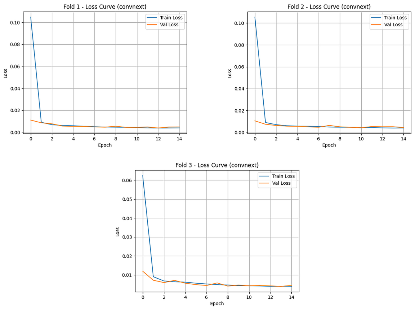
When the loss curves obtained during the training of the ConvNeXt network are examined, the rapid decrease observed in the training loss during the initial epochs indicates that the model adapts quickly to the dataset. In the subsequent epochs, both the training and validation losses remain at very low levels and stabilize with minimal fluctuations (
Figure 10).
The extremely small gap between the training and validation losses demonstrates that the model does not exhibit overfitting tendencies and possesses strong generalization capability. This observation indicates that the ConvNeXt architecture is effectively optimized on the given dataset and achieves a well-balanced learning process.
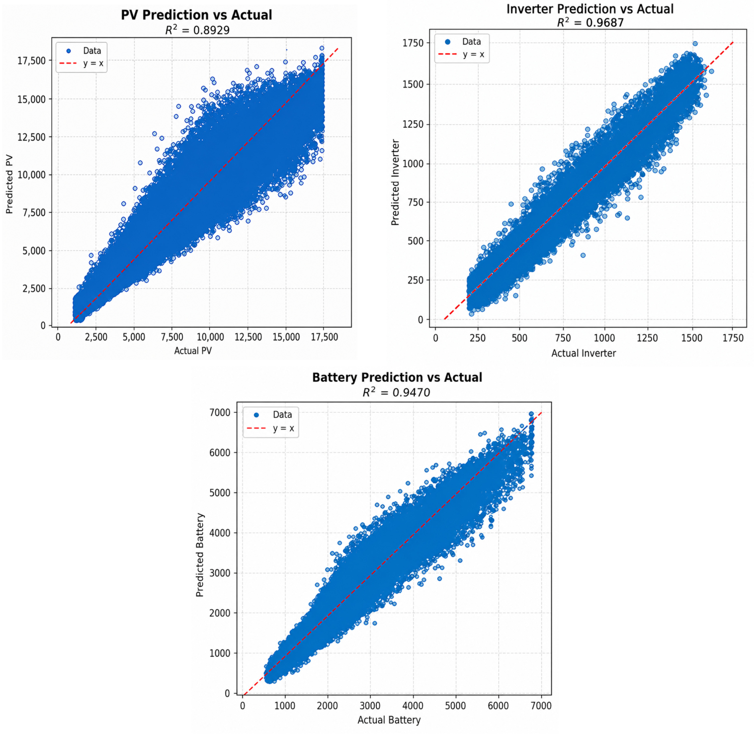
When the relationship between the photovoltaic (PV) values predicted by the trained ConvNeXt model and the actual PV values is examined, it can be observed from the plot that the predicted values are generally distributed close to the y = x line. This indicates that the model is capable of producing highly accurate predictions. In addition, the coefficient of determination reported in the plot is R
2 = 0.8929, showing that the model explains approximately 89% of the variance. This value represents a relatively high coefficient of determination in a regression context and supports the strong predictive capability of the model (
Figure 11).
However, a slight dispersion and deviation are observed in the predictions, particularly for large actual PV values (e.g., >15,000). This suggests that the model’s predictive performance may be somewhat limited for extreme (high) values. Nevertheless, the predictions exhibit a consistent and strong linear relationship across a wide data range. Overall, the ConvNeXt model is able to estimate actual PV values with high accuracy and effectively capture the underlying linear relationship. The model demonstrates strong generalization capability and is well suited for use in regression-based tasks of this nature.
When the prediction performance of the ConvNeXt model on inverter data is analyzed, the fact that the vast majority of predictions are closely aligned with the reference line clearly indicates that the model achieves high accuracy for inverter outputs. Deviations remain very low across most of the value range, and the distribution appears highly compact.
The coefficient of determination reported in the plot is R2 = 0.9846, indicating that the model explains 98.46% of the variance. This represents an exceptionally high level of accuracy from a statistical perspective and demonstrates that the ConvNeXt architecture fits the inverter data extremely well. The ConvNeXt model exhibits outstanding predictive performance for inverter values, establishing an almost one-to-one correspondence between predicted and actual values. This confirms that the model can be used reliably and consistently for regression-based tasks such as inverter capacity prediction.
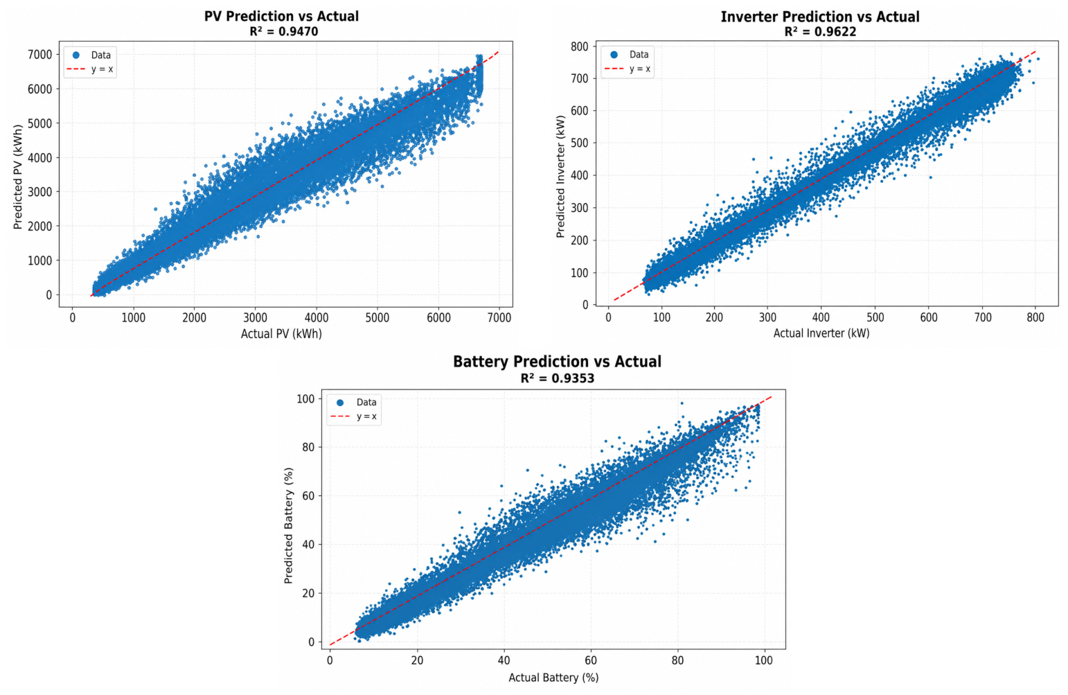
An examination of the ConvNeXt model’s prediction performance on battery data shows that the data points are generally located close to the reference line, indicating high prediction accuracy. However, compared to the inverter plot, the dispersion of data points is somewhat greater in this case. This suggests the presence of minor prediction deviations, particularly in the mid-to-upper value range, where the model occasionally exhibits slight linear deviations.
The coefficient of determination presented in the plot is R2 = 0.9470, meaning that the model explains 94.7% of the variance. This corresponds to a very high level of accuracy and demonstrates that the model exhibits strong generalization capability on battery data. The ConvNeXt-based model shows high performance in battery prediction tasks. Although the predictions are slightly more dispersed than those for inverter data, the overall accuracy remains statistically satisfactory. These results indicate that the model can also be effectively applied to regression problems related to battery systems.
Influenced by transformer-based design principles, ConvNeXt demonstrates strong generalization capability. High performance is achieved particularly in inverter (94.14%) and battery number (90.19%) predictions, while an acceptable level of accuracy (86.34%) is also observed for PV panel number estimation. Overall, ConvNeXt provides a robust architecture that, with its modern design, is capable of successfully modeling deep and complex relationships.
3.5. EfficientNet Results
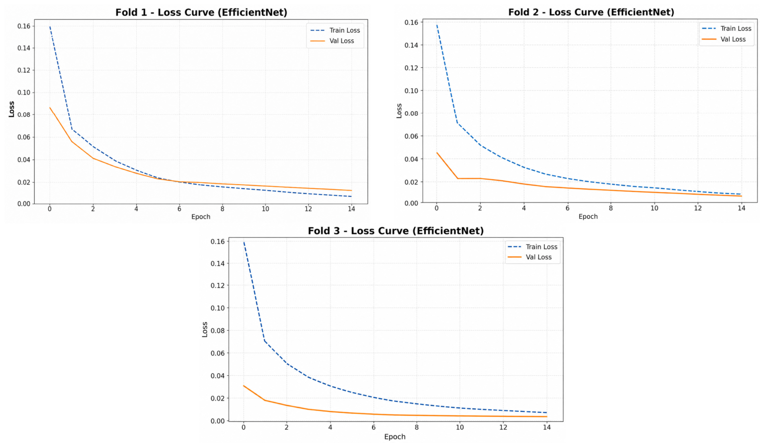
When the training and validation loss values obtained throughout the training process of the EfficientNet-based model are examined, the training loss curve (blue line) exhibits a continuous decreasing trend starting from the first epoch, indicating that the model progressively reduces its error on the training data. The validation loss (orange line) starts at a lower level compared to the training loss and shows a more rapid improvement during the initial epochs. Subsequently, the training and validation losses converge and nearly overlap from around the 10th epoch onward (
Figure 12).
This convergence indicates that the model demonstrates similar performance on both the training and validation datasets and does not exhibit overfitting tendencies. The minor variations (fluctuations) observed in the validation loss during the final epochs are very limited, suggesting that the model completes the learning process in a stable and well-controlled manner.
The EfficientNet model is able to generate meaningful predictions for PV outputs; however, the achieved accuracy remains limited. Although the linear relationship is relatively strong, the deviations observed at higher values and the moderate R
2 score indicate that the model has limitations in capturing the nonlinear structures present in PV data. In this context, while the EfficientNet architecture can be employed for photovoltaic panel number prediction tasks, it does not achieve the same level of predictive performance as the ConvNeXt architecture on this particular dataset (
Figure 13).
In contrast, the EfficientNet architecture exhibits high accuracy and stability in inverter prediction tasks. An R2 value exceeding 0.98 indicates strong generalization capability and demonstrates that the model successfully learns the linear relationship inherent in inverter data. The close alignment of predictions with the reference line further suggests that the model is largely free from systematic bias.
These findings indicate that the EfficientNet model achieves a level of performance comparable to ConvNeXt for regression-based tasks related to inverter systems.
For battery prediction tasks, the EfficientNet architecture also demonstrates highly successful performance. In particular, the high R2 value confirms the model’s strong regression capability on battery data. The overall distribution of predictions indicates that the model is able to generate reliable estimates across both low and high value ranges.
However, the predictions for battery data appear slightly more dispersed compared to those for inverter prediction. This may indicate greater variance or more complex underlying structures in the battery data. Nevertheless, overall, EfficientNet delivers a high level of predictive performance for these outputs.
EfficientNet is a high parameter-efficiency architecture designed based on the principle of scalability. The model’s ability to achieve 93.34% accuracy in inverter prediction confirms its computational efficiency. However, a decline in performance is observed for PV panel number estimation (83.95%). This suggests that the compound scaling strategy employed in the architectural design may have limited effectiveness for certain tasks.
3.6. SqueezeNet Results
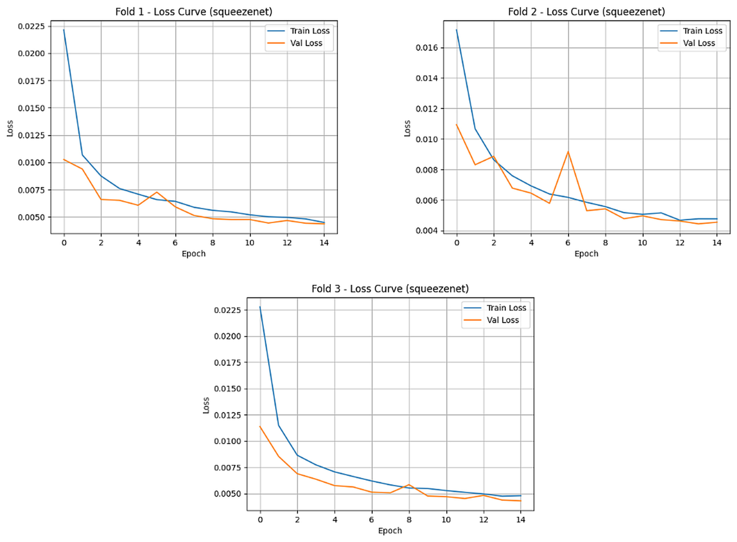
When the loss functions observed during the training process of the SqueezeNet architecture are examined, it is evident that SqueezeNet exhibits a stable and consistent training behavior for the given regression task. The parallel trends of the training and validation losses indicate that the model has good generalization capability and does not become overly dependent on the training data. Moreover, the low overall loss levels further support the model’s strong learning performance (
Figure 14).
These findings demonstrate that, despite its limited number of parameters, SqueezeNet is able to perform deep learning tasks efficiently. This performance is particularly noteworthy in terms of its suitability for embedded systems and resource-constrained environments.
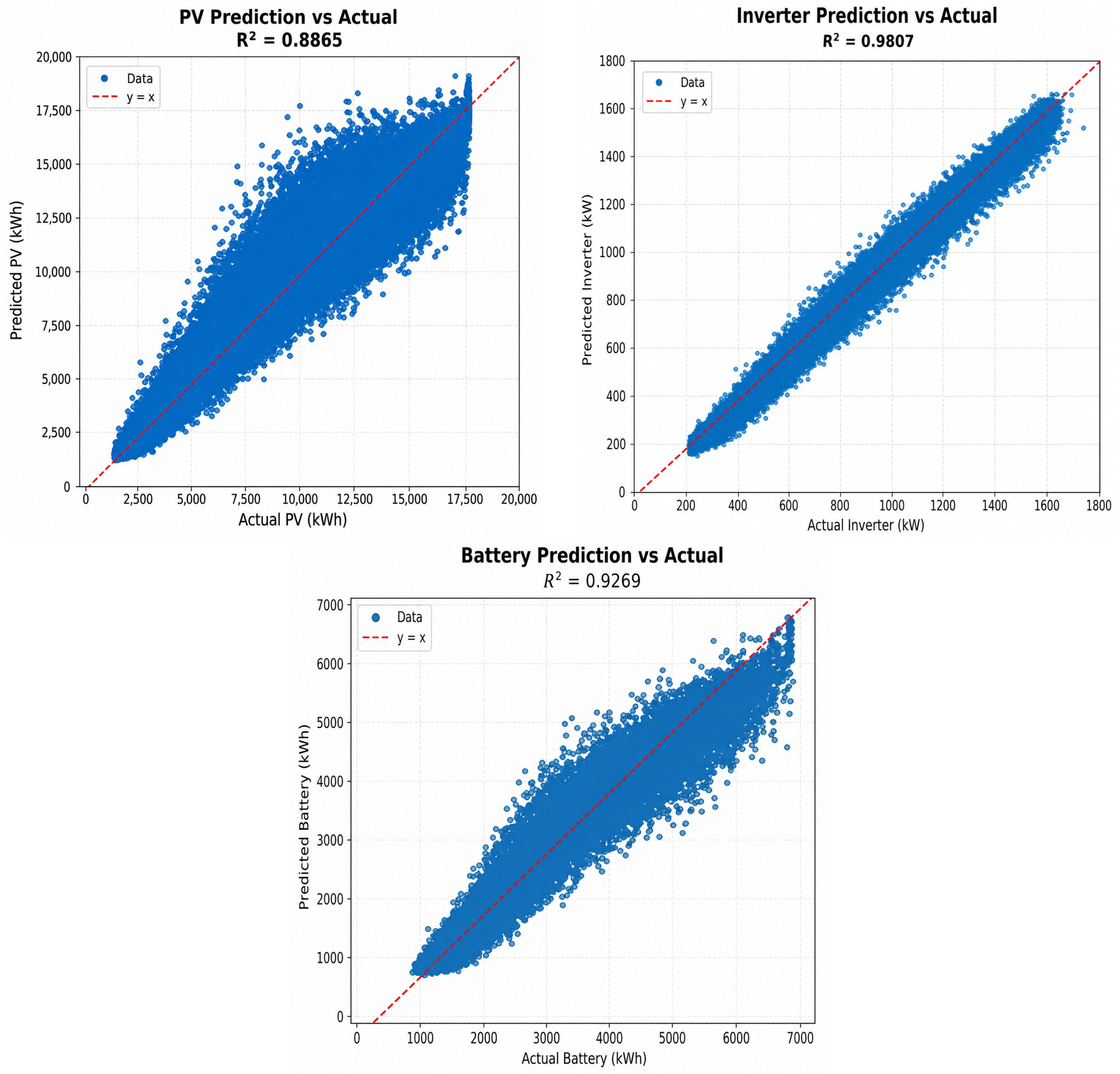
Despite its compact structure, the SqueezeNet architecture demonstrates satisfactory accuracy in the PV prediction task. In particular, the close alignment of the data distribution with the ideal prediction line supports the model’s overall generalization capability. Considering the simplicity of the model architecture, achieving this level of accuracy (high R
2) can be regarded as highly successful. Nevertheless, the dispersion observed at lower values—likely due to the inherent variability of environmentally sensitive systems such as PV—may indicate limited flexibility when compared to higher-capacity alternatives (
Figure 15).
The SqueezeNet model produces highly successful results in the inverter prediction task. The high coefficient of determination (R2) indicates strong learning and generalization capability on inverter data. Since inverter data tend to exhibit more distinct structural characteristics, even lightweight networks such as SqueezeNet are able to achieve high performance. These findings demonstrate that low-parameter deep learning architectures can still deliver high accuracy when combined with appropriate preprocessing and sufficient data. In this respect, SqueezeNet emerges as a viable alternative for inverter prediction, particularly in embedded systems or resource-constrained applications.
For the battery prediction task, the SqueezeNet model also exhibits satisfactory performance. Although greater dispersion among predictions is observed compared to inverter estimation, the high R2 value indicates strong generalization capability. The battery data likely exhibit higher variance and more complex distributions, which may have made this prediction task more challenging for the model. In this context, deeper or higher-parameter architectures could potentially provide additional benefits for battery prediction.
Nevertheless, the ability of compact models such as SqueezeNet to achieve such high accuracy with low computational cost demonstrates that they offer efficient and practical solutions for energy forecasting systems.
SqueezeNet is an extremely compact network with a very low number of parameters. Despite its lightweight architecture, it achieved a high accuracy of 93.43% in inverter power estimation. The prediction performances for battery count and photovoltaic (PV) panel count are also at acceptable levels. These results demonstrate that lightweight architectures, when combined with appropriate data representation, are capable of delivering strong and reliable performance.
3.7. Inception_V3 Results
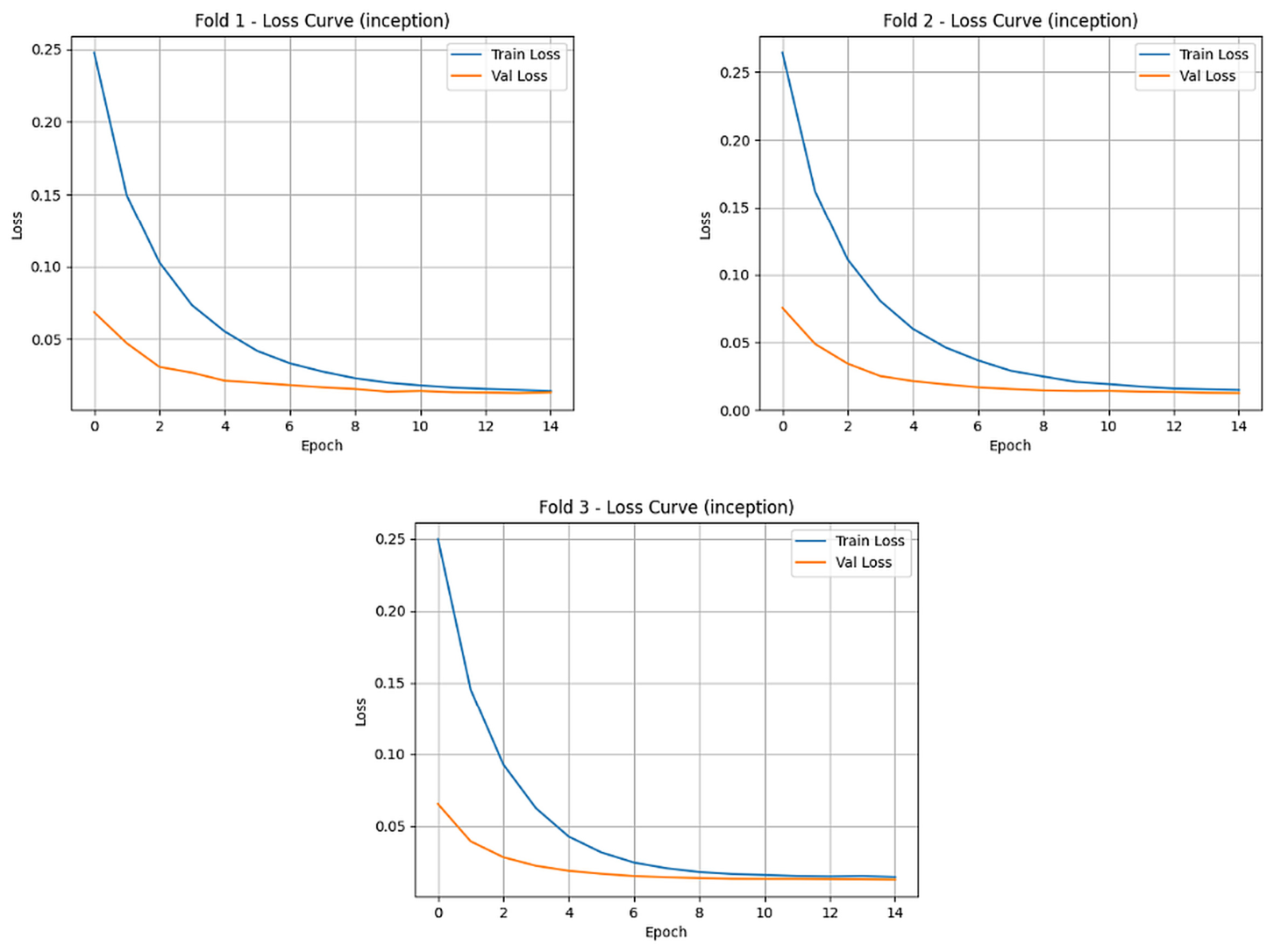
The Inception architecture exhibited a consistent and stable improvement throughout the training process on both the training and validation datasets. The close alignment of the corresponding loss curves indicates that the model preserved its generalization capability without overfitting to the training data (
Figure 16).
The pronounced decrease observed during the initial epochs suggests a rapid learning capability, reflecting the effectiveness of the multi-scale feature extraction mechanism inherent to the Inception architecture. In the subsequent epochs, the loss curves followed a more gradual and stable trend, indicating that the learning process converged and reached a steady state.
These findings demonstrate that the high-capacity structure of the Inception network was effectively optimized, enabling efficient training while avoiding overfitting. Overall, the Inception architecture achieved a balanced performance in terms of both learning capacity and generalization ability.
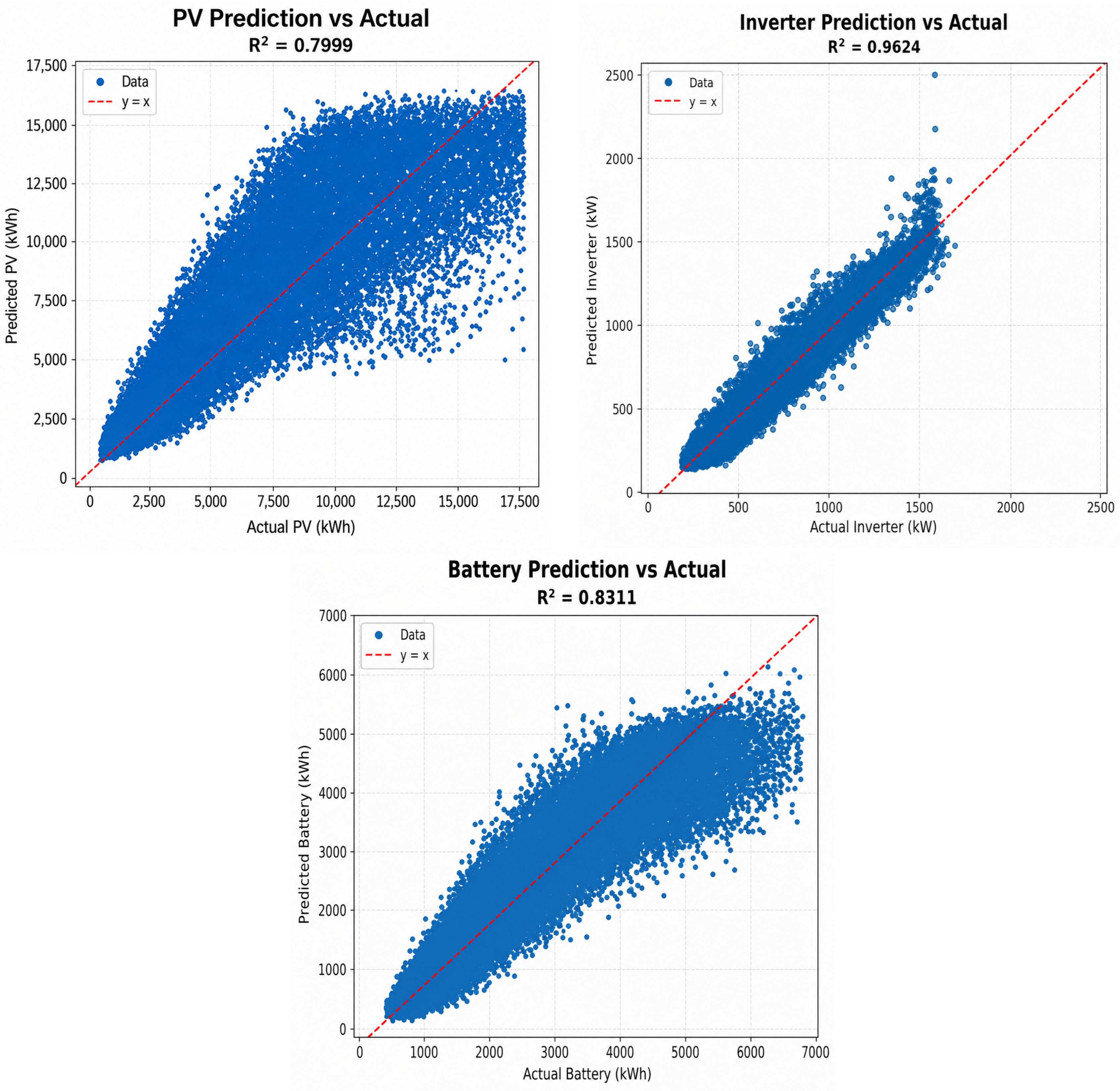
The Inception-based model demonstrates partially successful performance in photovoltaic (PV) prediction tasks. The predicted values exhibit a more scattered distribution, particularly at medium and high PV levels, where certain regions show systematic deviations. This behavior suggests that the model may struggle to accurately generalize higher PV values and may not fully capture the underlying nonlinear complexity of the data. The lower R
2 score compared to architectures such as EfficientNet or SqueezeNet further indicates that the Inception architecture is less suitable for PV prediction in this context (
Figure 17).
In contrast, the Inception architecture achieves high accuracy in the inverter prediction task. The corresponding plot shows that most data points are closely aligned with the ideal regression line, indicating that the model effectively learns both low and high inverter values.
For battery count prediction, the Inception model exhibits a moderate level of performance. However, compared to the other target variables, the prediction accuracy is relatively lower. In particular, increased dispersion and noticeable deviations at higher battery values are observed.
The Inception architecture is distinguished by its use of multi-scale filter structures. However, in this study, it did not achieve the expected performance in predicting the number of PV panels (80.93%) and battery units (83.0%). This outcome may be attributed to the architecture’s scale diversity being insufficiently aligned with the target variables in the context of the given problem. Nevertheless, the model achieved a reasonable level of performance in inverter prediction.
3.8. DenseNet121 Results
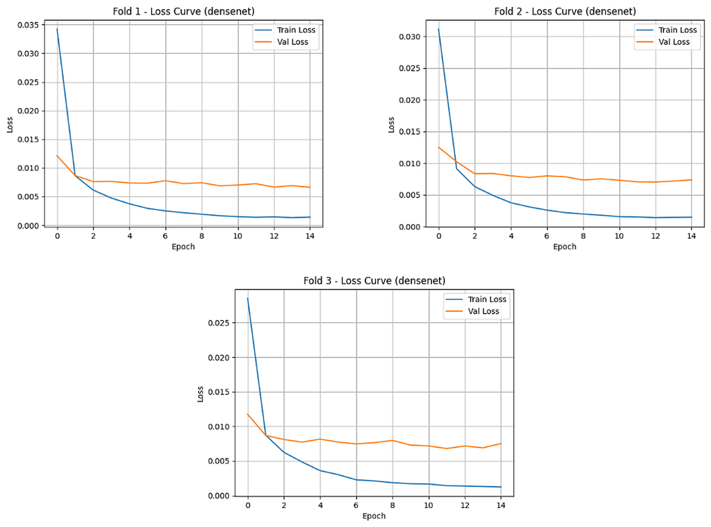
The DenseNet model exhibited a very strong fit to the training data; however, it showed early saturation on the validation dataset. This behavior suggests that the model is affected by overfitting, a common issue in high-capacity neural networks. Incorporating regularization techniques such as dropout, weight decay, and early stopping based on validation loss could help improve its generalization performance (
Figure 18).
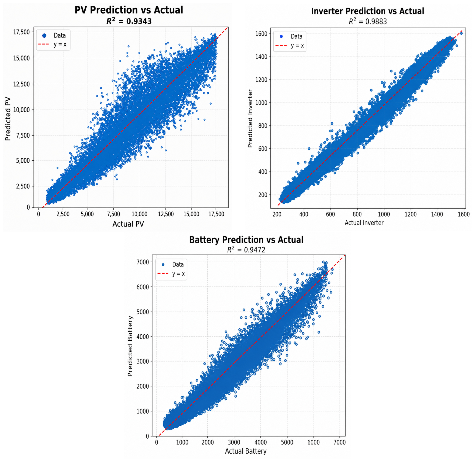
This model demonstrates a successful and reliable performance in predicting PV output power. The high accuracy (R
2 = 0.9343) and the well-distributed prediction pattern indicate that the model can be confidently utilized in real-world applications as well as in advanced optimization studies (
Figure 19).
The model achieves exceptionally high accuracy in inverter output prediction, highlighting its reliability for both laboratory-based analyses and field applications. Accurate estimation of inverter power is of critical importance for performance optimization in energy management systems, and the obtained results confirm the model’s suitability for such purposes.
Furthermore, the model provides statistically robust and reliable results in battery output prediction. Battery estimation plays a vital role in the planning and management of energy storage systems, and the achieved level of accuracy is highly promising for practical implementation.
DenseNet enables feature reuse and enhanced information flow through its densely connected layers. In this study, it achieved the highest accuracy in inverter power prediction (95.03%). Additionally, it reached very high accuracy levels in both PV panel count and battery count predictions, ranking second overall in average performance. These results demonstrate that the architecture possesses a strong representational capability and is highly effective for regression-based problems.
4. Conclusions and Recommendations
In this study, the output power of photovoltaic (PV), inverter, and battery systems was predicted using different deep learning architectures. The performance of the models was evaluated based on training and validation loss curves as well as prediction–ground truth comparison plots.
The results indicate that all architectures achieved a certain level of success in the respective prediction tasks. Among them, the DenseNet architecture stood out in terms of overall accuracy by achieving the highest R
2 scores across all output variables (PV, inverter, and battery). Specifically, DenseNet demonstrated strong correlations with R
2 values of 0.934, 0.9883, and 0.9472 for PV, inverter, and battery predictions, respectively. To facilitate comparison,
Table 3 consolidates the per-output percentage errors, coefficients of determination (R
2), and success rates of all eight evaluated architectures in a single overview, replacing the individual per-model summaries and eliminating the need for repetitive model-by-model reporting.
The Inception architecture exhibited moderate performance. While it produced successful results particularly in inverter power prediction, lower correlations were observed for PV and battery predictions compared to DenseNet, with R2(PV) = 0.7999 and R2(Battery) = 0.8311.
Despite its compact architectural design, SqueezeNet delivered notably strong results in inverter and battery predictions (R2(Inverter) = 0.9807, R2(Battery) = 0.9269). However, its performance in PV prediction was relatively limited compared to the other models (R2 = 0.8865).
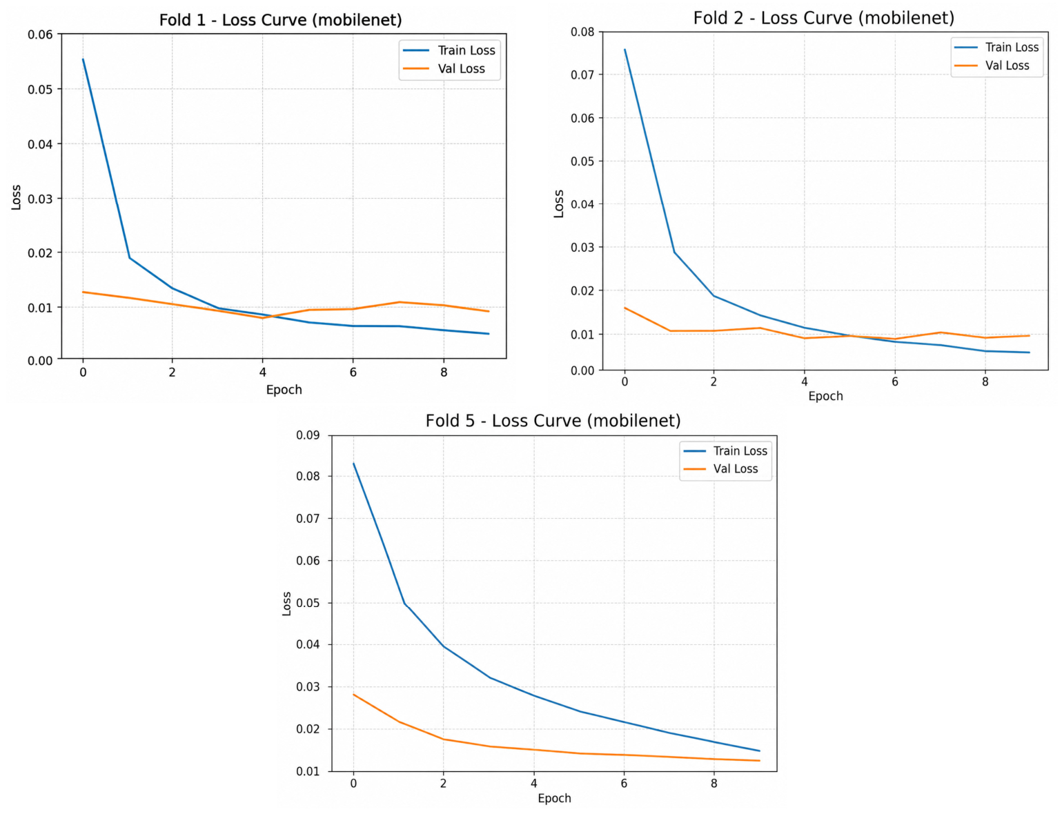
An examination of the loss curves revealed that training losses decreased steadily across all models, while validation losses reached early saturation depending on the architecture. This observation highlights the need for caution against overfitting, particularly in more complex architectures.
In conclusion, this study demonstrates that deep learning-based approaches are capable of predicting the output power of PV, inverter, and battery systems with high accuracy. In particular, the DenseNet architecture emerges as a strong candidate for such applications due to its superior predictive performance across all components. These findings suggest that deep learning can be effectively utilized in energy management systems and predictive maintenance applications.
In conclusion, DenseNet121 emerges as the architecture exhibiting the best overall performance for solving this problem, achieving the highest R2 values across all three outputs (PV, inverter, and battery), with ResNet performing comparably and yielding the best result for inverter capacity prediction (R2 = 0.9834). ConvNeXt follows closely behind these two models, delivering strong results with its modern architectural design. Lightweight networks such as SqueezeNet and MobileNet produced noteworthy outcomes, particularly for resource-constrained systems. In contrast, InceptionV3 was unable to sufficiently leverage its multi-scale architectural advantage within the context of this study.