An Uncertainty-Aware Kernel-Based Method for Regression: The Generalized Least Squares Support Vector Machine

Abstract

A robust evaluation of predictive uncertainty is essential for deploying machine learning models in high-risk sectors. While various techniques such as Gaussian Processes and Bayesian Neural Networks have been considered to address model uncertainty, the measurement uncertainty associated with input data, particularly regarding heteroscedasticity and autocorrelation, is often overlooked. This work introduces the Generalized Least Squares Support Vector Machine (GLS-SVM), a kernel-based regression model designed to integrate the full variance–covariance matrix of the response variable into the training process. A GUM-consistent methodology was developed for evaluating prediction uncertainty, including a correction for model bias. The model’s performance was validated against standard Least Squares Support Vector Machines (LS-SVMs) and Gaussian Processes (GPs) through two case studies: a simulated regression problem with correlated data and the calibration of a mass flow controller. Performance was quantified using a comparability index ($C_{\mathrm{index}}$), defined as the absolute error of the prediction weighted by its expanded uncertainty. Results demonstrated that, in the simulated case study, the GLS-SVM achieved a $C_{\mathrm{index}}$ consistently below 0.65, indicating that its predictions are statistically consistent with the ground truth. In contrast, competing models significantly exceeded unity, with peak values near 8, indicating a failure to provide physically consistent estimations. For the calibration of the mass flow controller, the GP models produced uncertainties one to three orders of magnitude smaller than the measurement uncertainties, whereas GLS-SVM yielded uncertainties that were more physically consistent with the underlying measurement process. Eventually, the proposed approach offers a versatile, metrologically informed framework for data-driven regression tasks where measurement covariance information is available and rigorous uncertainty quantification is required.

1. Introduction

Machine learning (ML) and deep learning (DL) models have become increasingly prevalent in both research and industry due to their ability to learn complex interactions among variables without requiring explicit models based on physical or empirical prior knowledge. A robust evaluation of predictive uncertainty is essential for deploying these models in high-risk sectors, such as health care [1,2], structural engineering [3,4], or early-warning systems [5]. In recent years, significant research effort has been dedicated to assessing uncertainties in ML/DL models [6,7,8]. Various techniques have been developed [9,10,11,12], the most popular ones being ensemble methods [13], Bayesian Neural Networks (BNNs) [14] and Monte Carlo Dropout [15], capable of evaluating and propagating the uncertainty of the neural network weights, and Gaussian Processes (GPs), which intrinsically provide prediction uncertainty [16] and have recently been combined in network structures or used in combination with neural networks [17,18]. Despite these progresses, the measurement uncertainty associated with input data is often overlooked. While some seminal works have addressed this issue by focusing on GPs, specifically regarding the integration of input uncertainty during training [19,20,21,22,23,24] and its subsequent propagation through the model, these efforts remain a minority. Furthermore, the existing literature often treats such cases under the general umbrella of ’noisy input data’ rather than formally addressing measurement results characterized by rigorous measurement uncertainty.

ML/DL models have also attracted the attention of the metrological community, especially when used for regression tasks. The reason is that there are many scenarios in which it is not possible to build or perform computations on an analytical model based on physical understanding, with data-driven approaches being the only available possibility [25]. The challenge behind the reliable assessment of uncertainty encouraged metrologists to investigate new methods to train uncertainty-aware models and to propagate uncertainty through ML models, in line with the Strategic Research Agenda (SRA) [26] of the European Metrology Network for Mathematics and Statistics (EMN Mathmet). Recently, the JCGM-WG1 also emphasized the growing intersection of Artificial Intelligence and measurement uncertainty [27]. The Working Group highlighted the urgent need for a unified metrological language for AI and a framework to ensure quality control for algorithmic inputs and outputs.

Recent publications from the metrology community deal with kernel methods [28,29,30,31] because of their tractable and more interpretable mathematics compared to DL models. The present work lies in this context and aims to point out how well-established statistical methodologies in metrology can help develop uncertainty-aware ML regression models. A common approach employed by metrologists to estimate the parameters of a usual uncertainty-aware regression model is to include the (known) covariance matrix of the input measurements (of both the dependent and the independent variable) within the loss function of a least-squares minimization problem [32]. Closed-form solutions exist when the covariance matrix of the target variable (i.e., the dependent or response variable) is included, which is the so-called Generalized Least Squares (GLS) [33]. With this approach, it is possible to address the heteroscedasticity and autocorrelation of the response data by exploiting the information supplied by the covariance matrix.

The goal of this work is to the replicate GLS approach for an ML model. The Least Squares Support Vector Machine (LS-SVM) [34,35], a variant of the popular Support Vector Machine (SVM) [36], is the best candidate. The main difference from SVM is that LS-SVM is computed by solving a linear system of equations instead of a quadratic programming optimization problem, which can be considered one of the main reasons for its success. Even though one drawback of this approach is that it results in a non-sparse model, pruning techniques have been developed (see [37] for instance) and this aspect is not a problem when reasonably small datasets are used. The computational aspects and their mathematical formulation, more manageable than other ML models, have been the main factors leading to the choice of using LS-SVM as the base model for this work. The Generalized Least Squares Support Vector Machine (GLS-SVM) is proposed here, deriving the mathematical framework for its training and for the evaluation of the prediction uncertainty through classical uncertainty propagation rules, consistent with the Guide to the Expression of Uncertainty in Measurement (GUM) [38]. The model is then compared to other kernel methods capable of evaluating prediction uncertainties, such as Gaussian Processes (GPs) and the LS-SVM itself. The comparison is performed on two case studies: a regression problem based on simulated data and a calibration problem of a mass flow controller.

In the next sections, the LS-SVM is described, and then the GLS-SVM is derived, with comments on aspects related to its implementation. Then, the two case studies are described and the comparison results are reported and discussed.

2. Materials and Methods

2.1. General Assumptions

A training dataset $D={\{{\mathit{x}}_i,y_i\}}_{i=1}^N$ is composed of N measurement results of the independent d—dimensional quantity $\mathit{x}\in {\mathbb{R}}^{d\times 1}$ and of the response $y\in \mathbb{R}$. Assuming that $\mathit{x}$ is deterministic, i.e., not affected by uncertainty, the response variable Y, which is the random variable of which y is the available realizations, can be expressed in general terms as

$$Y=m\left(\mathit{x}\right)+E$$

(1)

where m is the model of interest we want to estimate and E is a random noise affecting the measurements. Applying a regression technique provides an estimate of the latent function m. This estimator, denoted as $\widehat{m}$, is a random variable whose distribution depends on the model coefficients, which are themselves subject to uncertainty. The uncertainty in $\widehat{m}$ is used to construct confidence intervals, representing the uncertainty in the expected (average) response for a given input. In contrast, prediction intervals incorporate the additional dispersion caused by inherent noise, whose parameters must be known a priori or estimated from the data [39]. This paper restricts its scope to confidence intervals that are related to the model’s epistemic uncertainty. Consequently, all subsequent references to predictions and their uncertainties pertain specifically to the estimator $\widehat{m}$ and its associated standard uncertainty.

2.2. Least Squares Support Vector Machines

LS-SVM is a popular kernel-based model that has been successfully employed in a variety of fields such as electronic circuit design [40], control system applications [41], predictive maintenance [42], time series forecasting [43,44,45], and the development of measurement systems [46,47]. Thanks to the simple mathematical formulation of the model, sensitivity analysis can be easily performed to understand the most relevant input features to be employed [48]. Furthermore, LS-SVM and GPs have been shown to be mathematically equivalent in terms of their predictive mean [16,35], but they stem from different theoretical frameworks: frequentist optimization and Bayesian inference, respectively.

The idea behind LS-SVM is to solve a ridge regression problem exploiting Lagrange multipliers which span a dual space [35]. In social science and econometrics, an equivalent model is known under the name kernel regularized least squares [49], obtained by solving the ridge regression problem in the primal space after having introduced the kernel matrix (defined below). Before reporting the optimization problem, the general regression model is introduced and defined as $y=\phi {\left(\mathit{x}\right)}^{\mathrm{T}}\mathit{\omega }+b+e$, where $\phi (·):{\mathbb{R}}^{d\times 1}\to {\mathbb{R}}^{n\times 1}$ is the map chosen by the user and employed to project the independent variable to a higher dimensional feature space (${\mathbb{R}}^{n\times 1}$); $\mathit{\omega }$ is the vector of n regression coefficients; b is an offset, often called bias in the ML field; and e is the error term, which follows a distribution $E\left(\mathit{x}\right)$, centered in zero, that may be heteroscedastic [50].

To find the unknown coefficients $\mathit{\omega }$ and b, an optimization problem must be solved to find the minimum of the chosen loss function. In the case of ridge regression, the function to be minimized, S, is the least squares loss function with a Tikhonov regularizer [51]. Then, the optimization problem expressed in matrix formulation is

$$\begin{array}{cc}\hfill \underset{\mathit{\omega },b}{min}S& ={\displaystyle \frac{1}{2}}{\mathit{\omega }}^{\mathrm{T}}\mathit{\omega }+{\displaystyle \frac{1}{2}}\gamma {\mathit{e}}^{\mathrm{T}}\mathit{e}\hfill \\ \hfill \mathrm{such}\mathrm{that}\mathit{y}& =\mathbf{\Phi }\mathit{\omega }+\mathbf{1}b+\mathit{e},\hfill \end{array}$$

(2)

where $\mathit{y}$ is a $N\times 1$ vector containing the observations of the response variable; $\mathbf{\Phi }$ is a matrix $N\times n$ having rows equal to $\phi {\left({\mathit{x}}_i\right)}^{\mathrm{T}}$; $\gamma$ is the hyperparameter that weighs the importance of the regularization term, usually tuned by cross-validation [52]; $\mathit{e}$ is an $N\times 1$ vector of i.i.d. errors; and the term $\mathbf{1}$ is an $N\times 1$ vector with all the entries equal to 1. The Lagrange multipliers, here identified by the $N\times 1$ vector $\mathit{\alpha }$, are introduced to construct the Lagrange function to be minimized for solving the constrained optimization problem:

$$\mathcal{L}={\displaystyle \frac{1}{2}}{\mathit{\omega }}^{\mathrm{T}}\mathit{\omega }+{\displaystyle \frac{1}{2}}\gamma {\mathit{e}}^{\mathrm{T}}\mathit{e}-{[\mathbf{\Phi }\mathit{\omega }+\mathbf{1}b+\mathit{e}-\mathit{y}]}^{\mathrm{T}}\mathit{\alpha }.$$

(3)

The Karush–Kuhn–Tucker (KKT) conditions for optimality are obtained by posing the derivative of $\mathcal{L}$ with respect to $\mathit{\omega }$, b, $\mathit{e}$ and $\mathit{\alpha }$ equal to zero [53]. Eventually, a linear system of $N+1$ dimensions is retrieved, whose solution makes it possible to compute the LS-SVM model in the dual space spanned by the Lagrange multipliers:

$$\left[\begin{array}{cc}0& {\mathbf{1}}^{\mathrm{T}}\\ \mathbf{1}& \mathit{K}+{\gamma }^{-1}\mathit{I}\end{array}\right]\left[\begin{array}{c}b\\ \mathit{\alpha }\end{array}\right]=\left[\begin{array}{c}0\\ \mathit{y}\end{array}\right].$$

(4)

The $\mathit{I}$ term is the $N\times N$ identity matrix, whereas $\mathit{K}$ is the kernel matrix, equal to $\mathbf{\Phi }{\mathbf{\Phi }}^{\mathrm{T}}$, which is the matrix containing all the inner products among features of the training dataset, hence having $N\times N$ dimensions. The advantage of kernel methods is that the nonlinear mapping into a feature space remains implicit. Leveraging Mercer’s theorem [54], any symmetric positive semidefinite kernel function can be utilized to compute the inner product of projected features. This approach, often referred to as the kernel trick, allows the $ij$-th entry of the kernel matrix to be calculated simply as $k({\mathit{x}}_i,{\mathit{x}}_j)$.

The mean prediction ${\widehat{m}}_p$ to new input data ${\mathit{x}}_{\mathit{p}}$ is obtained by applying the model with the estimated coefficients $\widehat{\mathit{\alpha }}$ and $\widehat{b}$. Considering $N_p$ new instances, the LS-SVM predictions are expressed by

$${\widehat{\mathit{m}}}_{\mathit{p}}={\mathit{K}}_{\mathit{p}}\widehat{\mathit{\alpha }}+\mathbf{1}\widehat{b}.$$

(5)

The kernel matrix ${\mathit{K}}_{\mathit{p}}$ has dimensions $N_p\times N$ and is calculated through the evaluation of the kernel function for each pair $({\mathit{x}}_{\mathit{pi}},{\mathit{x}}_{\mathit{j}})$ with $i=1,\dots ,N_p$ and $j=1,\dots ,N$. The prediction uncertainties for ${\widehat{\mathit{m}}}_{\mathit{p}}$ can be obtained by applying the approximate method described by De Brabanter et al. [50], considered in Section 3.1 for the comparison. Other works attempted to construct confidence and prediction intervals for LS-SVM [55,56], but none of them considered the uncertainty associated with data, as will be done in the next section.

2.3. Generalized Least Squares Support Vector Machine

The heteroscedasticity of the response variable is tackled for least squares models by including in the loss function a specific weight matrix, which is full or diagonal depending, respectively, on the presence or the absence of correlation among the measurements. In general, the squared error terms are weighed by the inverse of ${\mathit{V}}_{\mathit{y}}$, the variance–covariance matrix of $\mathit{y}$.

The GLS-SVM model is developed following a reasoning similar to that behind LS-SVM but modifying the loss function as follows:

$$S={\displaystyle \frac{1}{2}}{\mathit{\omega }}^{\mathrm{T}}\mathit{\omega }+{\displaystyle \frac{1}{2}}{\mathit{e}}^{\mathrm{T}}{{\mathit{V}}_{\mathit{y}}}^{-1}\mathit{e}.$$

(6)

The inclusion of the full variance–covariance matrix within the loss function provides a framework for metrologically informed regularization. While the standard regularization parameter $\gamma$ penalizes model complexity to prevent overfitting, the inclusion of ${{\mathit{V}}_{\mathit{y}}}^{-1}$ accounts for the reliability of each observation. From a numerical perspective, this approach improves the conditioning of the linear system: by weighting residuals by their reciprocal (squared) uncertainties, the model avoids the instabilities typically caused by heteroscedastic outliers or highly correlated observations, which in standard LS-SVM can lead to an ill-posed optimization problem. Effectively, ${\mathit{V}}_y$ serves as a pre-conditioner that aligns the optimization landscape with the underlying physical measurement process.

The practice of weighting squared error terms in the loss function has been previously explored: the use of weights based on the empirical distribution of data can help to train LS-SVM models robust to outliers [37,57]. On the other hand, attempts to address correlated errors are available [58,59]. However, there are no cases in the literature in which heteroscedasticity and correlation are addressed by including the full variance–covariance matrix of the observations during training, likely because they are rarely available in non-metrological contexts.

Thanks to the similarity with Equation (2), this loss function can also be minimized using Lagrange multipliers (detailed calculations in Appendix A). The linear KKT system is solved analogously to the system shown in Equation (4):

$$\left[\begin{array}{cc}0& {\mathbf{1}}^{\mathrm{T}}\\ \mathbf{1}& \mathit{K}+{\mathit{V}}_{\mathit{y}}\end{array}\right]\left[\begin{array}{c}b\\ \mathit{\alpha }\end{array}\right]=\left[\begin{array}{c}0\\ \mathit{y}\end{array}\right].$$

(7)

The difference with LS-SVM is that the $\gamma$-scaled identity matrix is substituted by ${\mathit{V}}_{\mathit{y}}$. With this method, the coefficients $\mathit{\alpha }$ and b are estimated including the information related to uncertainty and correlations among the observations of the response variable. Furthermore, the obtained estimates $\widehat{\mathit{\alpha }}$ and $\widehat{b}$ also have an associated variance–covariance matrix, which can be computed directly from ${\mathit{V}}_{\mathit{y}}$. This can be shown after rewriting the solution for $\widehat{\mathit{\alpha }}$ and $\widehat{b}$ in a different way (adapting the results from Appendix I in [50]):

$$\mathbf{\Omega }=\mathit{K}+{\mathit{V}}_{\mathit{y}}.$$

(8)

$$\widehat{b}={\displaystyle \frac{{\mathbf{1}}^{\mathrm{T}}{\mathbf{\Omega }}^{-1}}{{\mathbf{1}}^{\mathrm{T}}{\mathbf{\Omega }}^{-1}\mathbf{1}}}\mathit{y}={\mathit{q}}^{\mathrm{T}}\mathit{y}.$$

(9)

$$\widehat{\mathit{\alpha }}=\left({\mathbf{\Omega }}^{-1}-{\displaystyle \frac{{\mathbf{\Omega }}^{-1}\mathbf{1}{\mathbf{1}}^{\mathrm{T}}{\mathbf{\Omega }}^{-1}}{{\mathbf{1}}^{\mathrm{T}}{\mathbf{\Omega }}^{-1}\mathbf{1}}}\right)\mathit{y}=\mathit{Z}\mathit{y}.$$

(10)

The above equations can be retrieved thanks to the simple KKT system that needs to be solved. As is clear from Equations (9) and (10), $\widehat{\mathit{\alpha }}$ and $\widehat{b}$ can be directly expressed as linear combinations of measurements $\mathit{y}$, where $\mathit{q}$ and $\mathit{Z}$ are a vector and a matrix of numerical coefficients, respectively. The computation of the variance, covariance and cross-covariance becomes straightforward [60]:

$$\mathbb{V}\left[\widehat{\mathit{\alpha }}\right]=\mathit{Z}{\mathit{V}}_{\mathit{y}}{\mathit{Z}}^{\mathrm{T}}.$$

(11)

$$\mathbb{V}\left[\widehat{b}\right]={\mathit{q}}^{\mathrm{T}}{\mathit{V}}_{\mathit{y}}\mathit{q}.$$

(12)

$$\mathrm{Cov}[\widehat{\mathit{\alpha }},\widehat{b}]=\mathit{Z}{\mathit{V}}_{\mathit{y}}\mathit{q}.$$

(13)

Eventually, using Equations (11)–(13) it is possible to assemble a more general variance–covariance matrix of the vector of coefficients $\widehat{\mathit{c}}={[\widehat{\mathit{\alpha }},\widehat{b}]}^{\mathrm{T}}$, i.e.,

$${\mathit{V}}_{\widehat{\mathit{c}}}=\left[\begin{array}{cc}\mathbb{V}\left[\widehat{\mathit{\alpha }}\right]& \mathrm{Cov}[\widehat{\mathit{\alpha }},\widehat{b}]\\ \mathrm{Cov}{[\widehat{\mathit{\alpha }},\widehat{b}]}^{\mathrm{T}}& \mathbb{V}\left[\widehat{b}\right]\end{array}\right].$$

(14)

While Equations (11) and (12) were initially derived by De Brabanter et al. [50], Equations (13) and (14) represent novel contributions, providing essential information regarding the correlation among the estimated model coefficients.

GLS-SVM predictions can be computed using Equation (5), but for evaluating the uncertainty of the predictions it is useful to rewrite it in a different way exploiting Equations (9) and (10):

$${\widehat{\mathit{m}}}_{\mathit{p}}=({\mathit{K}}_{\mathit{p}}\mathit{Z}+\mathbf{1}{\mathit{q}}^{\mathrm{T}})\mathit{y}={\mathit{H}}_{\mathit{p}}\mathit{y}.$$

(15)

In this way, the predictions are directly related to the $\mathit{y}$ measurement results through the projection matrix ${\mathit{H}}_{\mathit{p}}$, which allows a much easier computation of the uncertainty associated with ${\widehat{\mathit{m}}}_{\mathit{p}}$. When ${\mathit{x}}_{\mathit{p}}=\mathit{x}$, it is convenient to define the projection matrix $\mathit{H}=(\mathit{K}\mathit{Z}+\mathbf{1}{\mathit{q}}^{\mathrm{T}})$, which is evaluated just using the training samples. Then, the mean predictions at the training points are evaluated by $\widehat{\mathit{m}}=\mathit{H}\mathit{y}$. Before any uncertainty evaluation, it is crucial to remove any bias from the predictions, as suggested by the GUM [38]. The evaluation of the bias is not straightforward and most of the time only an estimate can be computed. Using the approach described in [50], the bias for new predictions can be estimated as

$$\Delta {\widehat{\mathit{m}}}_{\mathit{p}}={\mathit{H}}_{\mathit{p}}\widehat{\mathit{m}}-{\widehat{\mathit{m}}}_{\mathit{p}}={\mathit{H}}_{\mathit{p}}\mathit{H}\mathit{y}-{\mathit{H}}_{\mathit{p}}\mathit{y}$$

(16)

Then, the corrected predictions can be expressed as

$${\widehat{\mathit{m}}}_{\mathit{p}}^{*}={\widehat{\mathit{m}}}_{\mathit{p}}-\Delta {\widehat{\mathit{m}}}_{\mathit{p}}={\mathit{H}}_{\mathit{p}}(2\mathit{I}-\mathit{H})\mathit{y}.$$

(17)

Even though in [50] the authors tried to remove the bias before computing confidence intervals, they only used the variance associated with ${\widehat{\mathit{m}}}_{\mathit{p}}$ without considering the uncertainty associated with the bias term. The more comprehensive approach, conforming to the GUM, is to evaluate the variance–covariance matrix of the corrected predictions (and mean values) directly from Equation (17):

$$\mathbb{V}\left[{\mathit{m}}_{\mathit{p}}^{*}\right]={\mathit{H}}_{\mathit{p}}(2\mathit{I}-\mathit{H}){\mathit{V}}_{\mathit{y}}{(2\mathit{I}-\mathit{H})}^{\mathrm{T}}{{\mathit{H}}_{\mathit{p}}}^{\mathrm{T}}.$$

(18)

The standard uncertainty of the point predictions and the corresponding average values are given by the square root of the diagonal of Equation (18), whereas the covariances among different predictions are retrieved from the off-diagonal elements. The evaluation of confidence intervals for a specific coverage probability necessitates defining the probability density function (PDF) of ${\mathit{m}}_{\mathit{p}}^{*}$. Given the assumption of Gaussian input quantities y, it is appropriate to model ${\mathit{m}}_{\mathit{p}}^{*}$ using a normal distribution, as it is derived from a linear combination of the observations $\mathit{y}$. Consequently, the quantiles associated with a target coverage probability are determined using a Gaussian PDF, characterized by a standard deviation equivalent to the standard uncertainty derived in Equation (18).

The proposed model has been implemented in MATLAB R2023b, paying particular attention to the tuning of the hyperparameters associated with the chosen kernel function. A dedicated $k_{\mathrm{CV}}$-fold cross-validation procedure is implemented by choosing as the optimization metric the Generalized Mean Square Error (GMSE), based on the Mahalanobis distance:

$$GMSE={\displaystyle \frac{1}{N_v}}{({\mathit{y}}_v-\widehat{m}\left({\mathit{x}}_{\mathit{v}}\right))}^{\mathrm{T}}{\mathit{V}}_{{\mathit{y}}_{\mathit{v}}}^{-\mathbf{1}}({\mathit{y}}_v-\widehat{m}\left({\mathit{x}}_{\mathit{v}}\right)),$$

(19)

where the subscript v indicates the set of quantities pertaining to the validation set used in each fold. This approach accounts for the underlying variance–covariance structure of the measurement results, providing a more rigorous validation than the commonly used root mean square error. Eventually, the tuned hyperparameters are used to train the model over the complete training dataset. The library for training GLS-SVM and performing predictions is publicly available (see the Data Availability Statement), and some additional details about the implementation are reported in Appendix B.

Note that the generalized kernel regularized least squares estimator introduced by Dang and Ullah [61] within the econometric literature is mathematically equivalent to the model proposed here. However, the formulation in [61] ignores the bias term b and the minimization problem is solved in the primal space. The GLS-SVM derived via the method of Lagrange multipliers, accounting also for the bias term, has not been previously reported.

2.4. Case Studies

To evaluate the performance of the proposed method, the GLS-SVM unbiased predictions are compared across two case studies with those obtained by using LS-SVM and Gaussian Process (GP) models. The LS-SVM training and predictions were obtained using the open-source library LS-SVMlab [62], version 1.8 run on MATLAB R2023b. In contrast, the GPs were developed using the scikit-learn library [63], version 1.7.2 run on Python 3.10.20, selected for its native support for heteroscedastic datasets. Two distinct GP models were trained: a standard model that disregards input measurement uncertainty and assumes a homoscedastic noise to be estimated from the training data, and another one that accounts for the heteroscedastic measurement uncertainty in the response variable during training (additional details are reported in the scikit-learn documentation). To ensure a fair comparison, all the ML models are trained considering the same kind of kernel function, chosen based on the addressed problem.

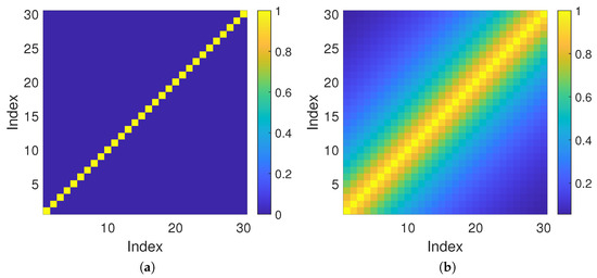
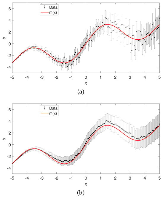
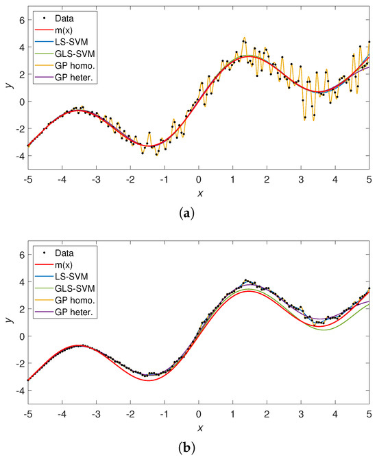
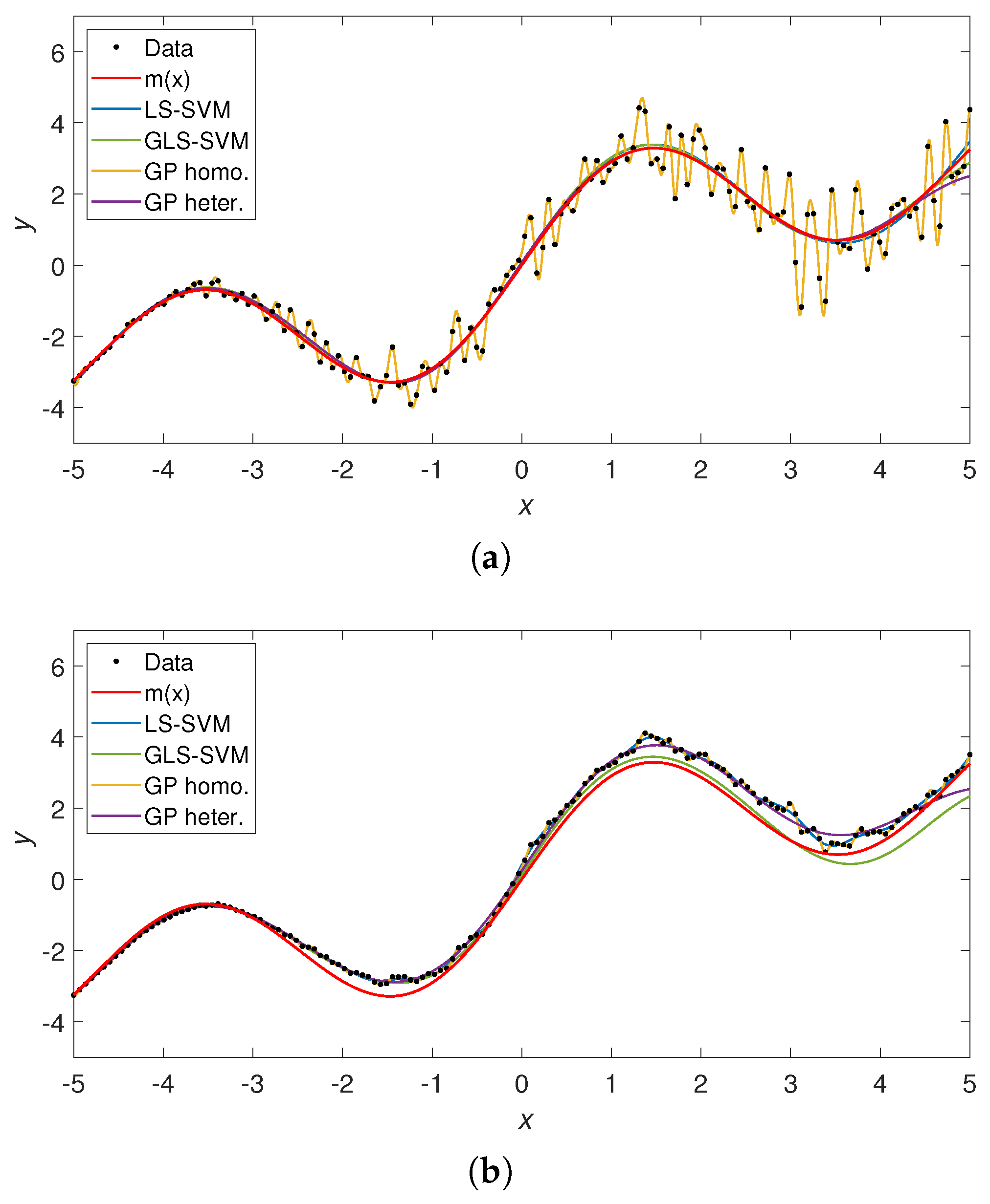
The first case study is a classical regression problem for the estimation of a function. The latent function, considered as the ground truth, is $m\left(x\right)={\displaystyle \frac{x}{5}}+2sin\left(4{\displaystyle \frac{x}{10}}\right)+2sin\left(13{\displaystyle \frac{x}{10}}\right)$, evaluated in the interval $[-5,5]$. The training dataset consists of $N=150$ pairs $(x,y)$, with input data x being regularly spaced in the specified domain. The response variable is instead sampled from a multivariate normal distribution having mean vector ${[m\left(x_1\right),\dots ,m\left(x_N\right)]}^{\mathrm{T}}$ and covariance matrix defined for the purpose. To test the model in the case of heteroscedastic and/or autocorrelated data, two different covariance matrices were defined, respectively. The first is a diagonal whose entries are the squared uncertainties. The heteroscedastic uncertainty was chosen to linearly increase between 0.01 and 1 in the domain, hence being $u\left(x\right)=0.01+{\displaystyle \frac{0.99}{10}}(x+5)$. The second covariance matrix is of Toeplitz kind [60], obtained by defining a decreasing exponential correlation function $\rho (y_i,y_j)=exp(-{\displaystyle \frac{|j-i|}{\tau }})$, where $\tau$ is a length scale chosen equal to 50 ($1/3$ of N). Figure 1 reports the two kinds of matrices, which are graphically shown considering a smaller dataset ($N=30$) for the sake of visualization, but maintaining the same proportion $\tau /N$ ($\tau =10$). The samples drawn from the corresponding multivariate normal distributions are shown in Figure 2.

Figure 1. Correlation matrix in cases of independent (a) and correlated data (b), considering $N=30$ and $\tau =10$.

Figure 2. (a) Heteroscedastic independent dataset. (b) Heteroscedastic and autocorrelated dataset. All the uncertainty bars are shown with a coverage factor $k=2$. The red line is the ground truth to estimate.

A Radial Basis Function (RBF) kernel is considered for this case study because it is universal, making it possible to approximate any function [54]. This kernel is characterized by a single hyperparameter ${\sigma }_h$ and has the following general form:

$$k({\mathit{x}}_i,{\mathit{x}}_j)=e^{-{\displaystyle \frac{{({\mathit{x}}_i-{\mathit{x}}_j)}^2}{{\sigma }_h^2}}}.$$

(20)

For GLS-SVM and LS-SVM a 10-fold cross-validation is considered for tuning the hyperparameters, which is the standard frequentist approach to prevent overfitting by identifying the optimal regularization and kernel parameters [35]. After cross-validation, the (G)LS-SVM models are trained over the complete dataset using the optimal hyperparameters. For GP models, the cross-validation is not required since the hyperparameters are obtained by maximizing the log-marginal-likelihood (LML) based on a passed optimizer, which is the standard Bayesian procedure for hyperparameter determination [16]. Although the tuning procedure is different, the comparison between the SVM and GP models is fair since they are trained using in both cases the complete set of training data. Eventually, the predictions and the associated uncertainties are evaluated for $N_p=1000$ equally spaced $x_p$ over the domain.

The second case study consists of a practical application of GLS-SVM to the calibration of a mass flow controller (MFC), described in [64] (example E3.3). The dataset is obtained from a calibration performed at the Italian National Metrology Institute (INRiM) against the primary standard for low flow rates (the INRiM Microgas station). The MFC is characterized in terms of its calibration coefficient $C=q_R/q_N$, where $q_R$ is the reference volume flow rate at standard conditions supplied by the MFC under calibration and read by the Microgas station, whereas $q_N$ is the nominal flow rate of the MFC. Since the flow rate is always read using the same reference, values of C at different nominal values are correlated and the corresponding full variance–covariance matrix should be considered during the estimation of the calibration curve. Indeed, the function $C\left(q_N\right)$ is generally obtained using the standard GLS regression, choosing a polynomial function of the following type:

$$C\left(q_N\right)={\displaystyle \frac{a_0}{q_N}}+{\displaystyle \frac{a_1}{\sqrt{q_N}}}+a_2+a_3\sqrt{q_N}+a_4{q}_N.$$

(21)

The experimental measurements C obtained during the calibration, along with the estimated values $\widehat{C}$ derived via the GLS fit, are summarized in Table 1 alongside their respective uncertainties. The regression coefficients were calculated using the Calibration Curve Computing Software release 1.3 [65], developed at INRiM. The GLS fit is here considered as the ground truth, since it is the state-of-the-art calibration model for MCFs at INRiM. The covariance matrix associated with C values, the vector estimate of GLS parameters and the corresponding covariance matrix needed to evaluate $\widehat{C}$ values and their uncertainties and correlations, are not reported here, but they are fully available at the shared repository (see the Data Availability Statement).

Table 1. Calibration dataset of a mass flow controller calibrated at nominal flow rate values $q_N$ against the INRiM primary standard. C represents the (dimensionless) measurement values. The fitted values $\widehat{C}$ are obtained through GLS regression of Equation (21). The reported values for $u\left(C\right)$ and $u\left(\widehat{C}\right)$ are standard uncertainties.

${\mathit{q}}_{\mathit{N}}\mathbf{/}\mathbf{\left(}{\mathbf{cm}}^{\mathbf{3}}{\mathbf{min}}^{\mathbf{-}\mathbf{1}}\mathbf{\right)}$	C	$\mathit{u}\left(\mathit{C}\right)$	$\widehat{\mathit{C}}$	$\mathit{u}\left(\widehat{\mathit{C}}\right)$
100	0.8485	0.0013	0.8483	0.0013
200	0.9296	0.0005	0.9298	0.0005
350	0.9602	0.0008	0.9597	0.0006
600	0.9787	0.0006	0.9782	0.0003
900	0.9880	0.0004	0.9890	0.0003
1200	0.9951	0.0004	0.9944	0.0003
1500	0.9962	0.0003	0.9963	0.0003

GLS-SVM is employed in this specific context to find a regression function without making any assumption on the functional form. Because polynomials can describe well the relation between C and $q_N$, a polynomial kernel is considered here, for both SVM and GP models, which has the following general expression:

$$k({\mathit{x}}_{\mathit{i}},{\mathit{x}}_{\mathit{j}})={({{\mathit{x}}_{\mathit{i}}}^{\mathrm{T}}{\mathit{x}}_{\mathit{j}}+t)}^p,$$

(22)

where hyperparameters t and p are tuned by a 6-fold cross-validation, equivalent in this case to a leave-one-out cross-validation (LOOCV).

3. Results and Discussion

The results of two case studies are reported here for the function estimation problem in Section 3.1 and the MFC calibration in Section 3.2.

3.1. Function Estimation

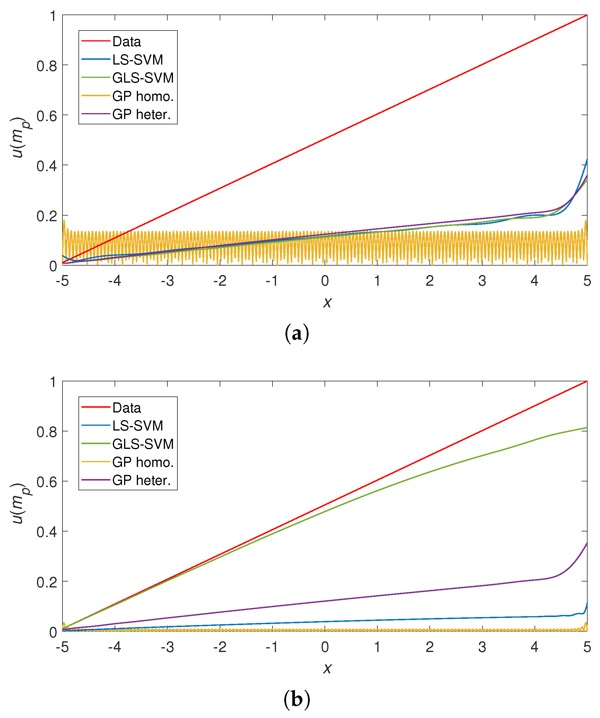
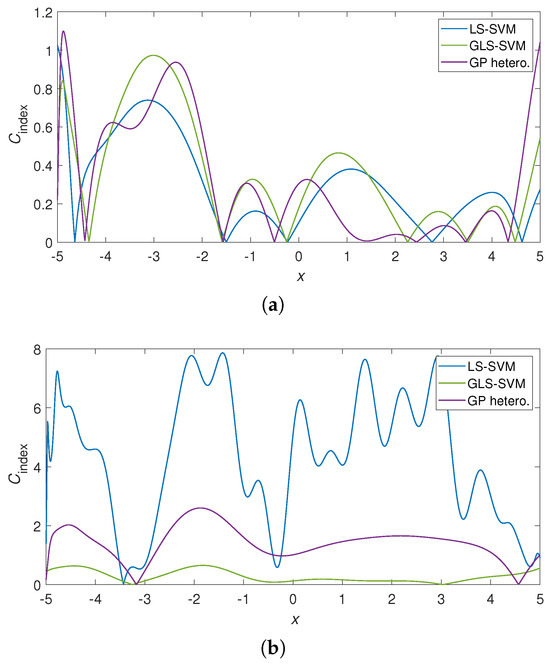
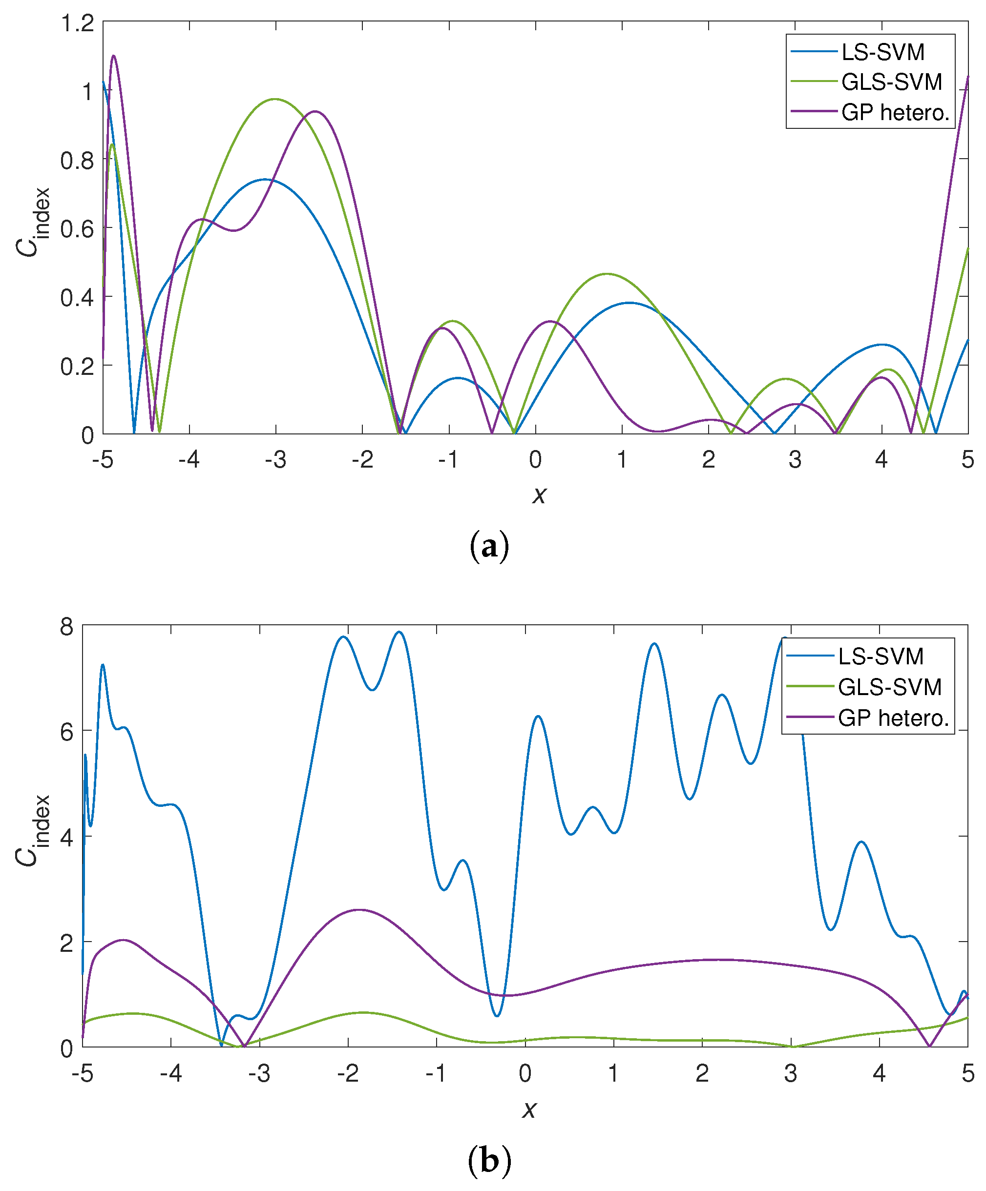
The predictions of the considered ML models are shown in Figure 3 for both independent and correlated data, whereas the prediction uncertainties are shown in Figure 4. To evaluate how well the models were capable of reproducing the underlying latent function, a comparability index was defined at each prediction point $x_p$ for the corresponding predicted value $\widehat{m_p}$:

$$C_{\mathrm{index}}\left(x_p\right)={\displaystyle \frac{|\widehat{m_p}-m\left(x_p\right)|}{k·u\left(\widehat{m_p}\right)}},$$

(23)

where $x_p$ runs over the whole domain of interest and the corresponding ground truth value $m\left(x_p\right)$ is considered with no uncertainty. This index is the absolute error of the prediction, weighted by its expanded uncertainty ($k=2$ is considered). The results of this evaluation are shown in Figure 5. Note that, to simplify the notation, the symbol ${\widehat{m}}_p$ in Equation (23) denotes unbiased predictions for (G)LS-SVM, whereas it corresponds to bias values for GP models. This convention is adopted throughout the remainder of this work.

Figure 3. Comparison of the predictions among the considered ML models trained on heteroscedastic-independent (a) and heteroscedastic-correlated data (b).

Figure 4. Comparison of the prediction standard uncertainties ($k=1$) among the considered ML models trained on heteroscedastic-independent (a) and heteroscedastic-correlated data (b). The red line reports the input parametrized uncertainty considered for training.

Figure 5. Comparability index of the ML predictions for heteroscedastic-independent (a) and heteroscedastic-correlated data (b).

Beginning with the independent case analysis, the only model that failed to achieve satisfactory performance was the homoscedastic GP, which was trained without considering input uncertainties. This model exhibited significant overfitting, resulting in an interpolation that deviated substantially from the latent function. Furthermore, its predictive uncertainties displayed an oscillatory behavior between 0 and 0.14 across the domain, causing the comparability index to fluctuate between 0 and 581, with an extreme outlier reaching 55,940.5 at the final data point. Consequently, the $C_{\mathrm{index}}$ for this model is omitted from Figure 5a for clarity. Conversely, the LS-SVM, GLS-SVM, and heteroscedastic GP successfully recovered the latent function. For these models, predictive uncertainties increased linearly with input uncertainty, albeit at a lower rate, with a more pronounced increase observed in the interval $[4.5,5]$. For these models, the comparability index remains predominantly below unity—except for certain predictions at the domain boundaries—and vanishes at the intersection points between the predictions and the latent function. This evaluation confirms that, for independent data, kernel-based methods maintain robust performance even when input uncertainties are not explicitly incorporated during training, as demonstrated by the LS-SVM.

In the presence of correlated data, for $x<0$ the models tend to agree due to the relatively small input uncertainties; however, they deviate significantly for $x\ge 0$.

The homoscedastic GP continues overfitting the observations—an effect less discernible in Figure 3b, yet present. The model produces nearly null uncertainties—a result that is non-physical and inconsistent with the a priori information on the dataset. Corresponding compatibility index values are huge and not even reported in Figure 5b.

The LS-SVM model tracks the local data patterns closely and it fails to accurately reconstruct the ground truth. Its uncertainties are smaller than those in the independent scenario, resulting in a comparability index that oscillates predominantly above one, peaking at approximately 8.

The heteroscedastic GP also tends to follow the data, departing from the reference function. However, it results in a slightly better comparability index ($C_{\mathrm{index}}$ values ranging between 1 and 2.6), despite the omission of input correlations during training.

The GLS-SVM definitely provides the most accurate estimation of $m\left(x\right)$, yielding predictive uncertainties that are larger than those of the LS-SVM and GP and showing a much smaller comparability index, always less than 0.65. The increase in its prediction uncertainty with respect to the other models is meaningful, as the GLS-SVM successfully incorporates the full data correlation structure.

3.2. Calibration of a Mass Flow Controller

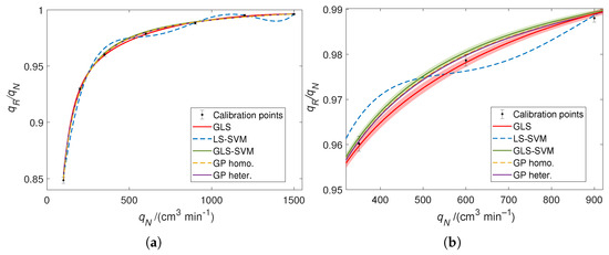
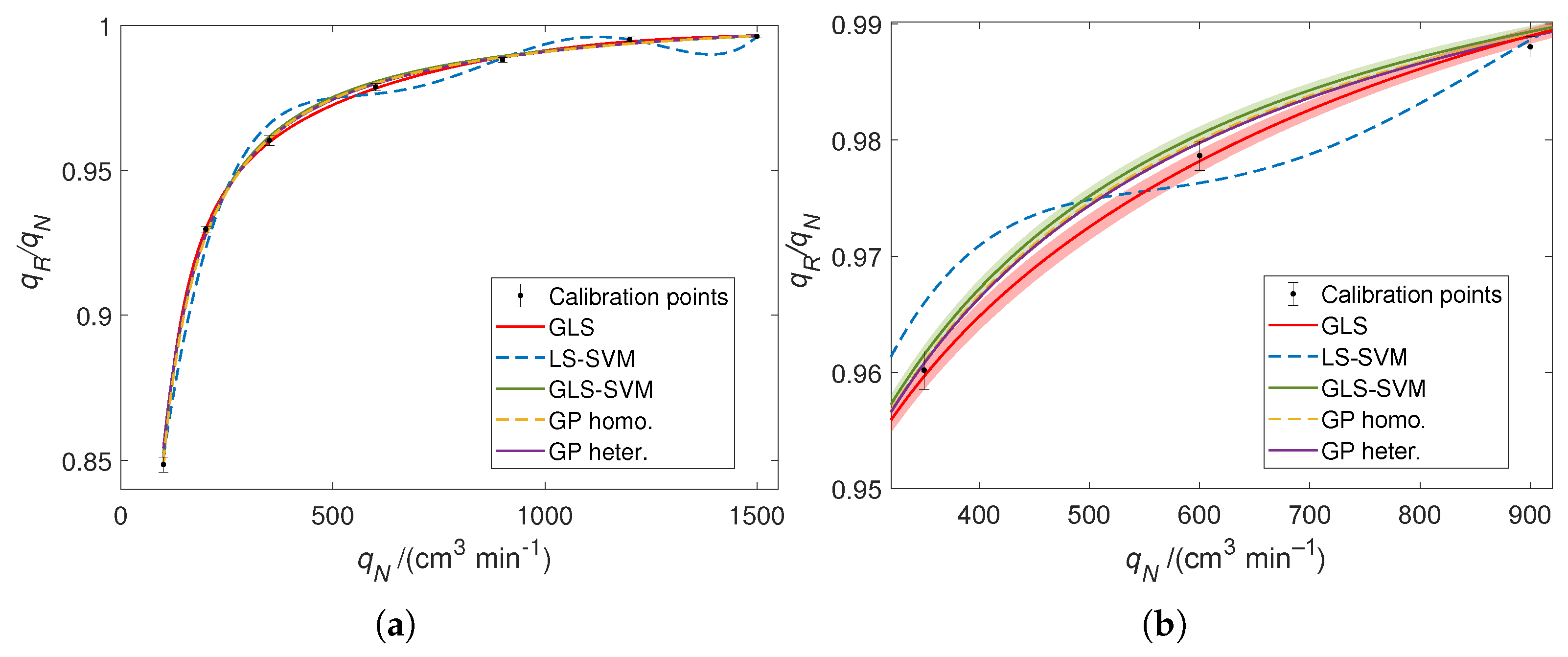
The comparison between the GLS calibration curve and the LS-SVM, GLS-SVM, and GP regressions is illustrated in Figure 6. Although the LS-SVM predictions are plotted, their associated uncertainties are omitted due to numerical divergence, with values reaching orders of ${10}^{14}$. Furthermore, the LS-SVM deviates significantly from the GLS reference, exhibiting spurious oscillations between calibration points; these non-physical artifacts necessitated the exclusion of the model from further comparative analysis. In contrast, the confidence intervals for the GP models are barely discernible in the figure. This is due to their significantly lower uncertainty values, one and three orders of magnitude smaller for the heteroscedastic and homoscedastic GPs, respectively, compared to the GLS and GLS-SVM results (see Table 2). While the prediction curves for the GLS-SVM and both GP variants are largely consistent with the reference, localized deviations occur for $q_N$ between 400 and 900 cm³ min⁻¹, as highlighted in the detail of Figure 6b.

Figure 6. (a) Calibration curves of a mass flow controller obtained with standard GLS fit (reference), LS-SVM and GLS-SVM. Confidence bands ($k=2$) are also plotted and better visualized in panel (b), which shows a zoom of the fit. The confidence bands for LS-SVM are not reported since they diverged towards values of orders of magnitude larger than 1. For GPs, the bands are too small to be visible.

Table 2. Predictions of the ML models with the associated standard uncertainties, over the calibration dataset reported in Table 1.

	GLS-SVM		GP Homo.		GP Heter.
${\mathit{q}}_{\mathit{N}}\mathbf{/}\mathbf{\left(}{\mathbf{cm}}^{\mathbf{3}}{\mathbf{min}}^{\mathbf{-}\mathbf{1}}\mathbf{\right)}$	$\hat{\mathit{C}}$	$\mathit{u}\mathbf{\left(}\hat{\mathit{C}}\mathbf{\right)}$	$\hat{\mathit{C}}$	$\mathit{u}\mathbf{\left(}\hat{\mathit{C}}\mathbf{\right)}$	$\hat{\mathit{C}}$	$\mathit{u}\mathbf{\left(}\hat{\mathit{C}}\mathbf{\right)}$
100	0.8524	11 × 10−4	0.8493	4.5 × 10−7	0.8541	3.0 × 10−5
200	0.9279	4.0 × 10−4	0.9271	2.1 × 10−7	0.9278	1.7 × 10−5
350	0.9615	3.9 × 10−4	0.9609	1.8 × 10−7	0.9608	7.7 × 10−6
600	0.9805	3.3 × 10−4	0.9800	2.0 × 10−7	0.9798	7.5 × 10−6
900	0.9893	2.4 × 10−4	0.9890	2.2 × 10−7	0.9889	8.4 × 10−6
1200	0.9937	2.0 × 10−4	0.9936	2.3 × 10−7	0.9936	8.9 × 10−6
1500	0.9963	2.3 × 10−4	0.9964	2.4 × 10−7	0.9965	9.2 × 10−6

For the purpose of evaluating the consistency between models and GLS, the following comparability index is defined:

$$C_{\mathrm{index}}={\displaystyle \frac{|{\widehat{C}}_{\mathrm{ML}}-{\widehat{C}}_{\mathrm{GLS}}|}{k·\sqrt{u^2\left({\widehat{C}}_{\mathrm{ML}}\right)+u^2\left({\widehat{m}}_{\mathrm{GLS}}\right)}}},$$

(24)

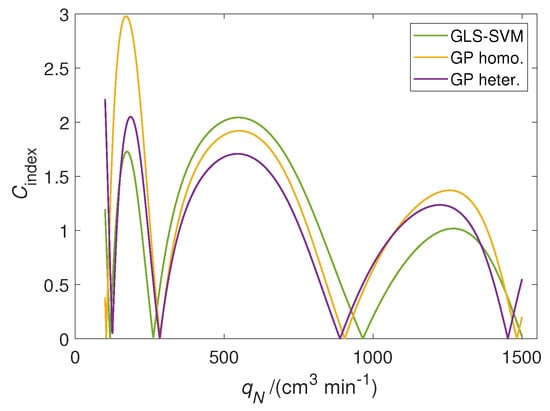
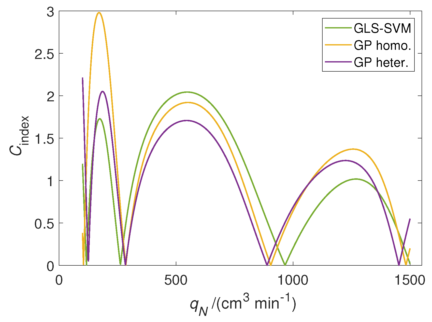
where ${\widehat{C}}_{\mathrm{ML}}$ is the prediction performed with one of the ML models, which is compared with ${\widehat{C}}_{\mathrm{GLS}}$, the GLS estimate. The coverage factor ($k=2$) multiplies the error uncertainty, which in this case also accounts for the uncertainty of the GLS fit. The evaluation of the comparability index is illustrated in Figure 7, revealing that the index exceeds unity for all models across various regions of the calibration domain. The GLS-SVM reaches a maximum value of approximately 2 at a nominal flow rate of 550 cm³ min⁻¹. In contrast, the homoscedastic and heteroscedastic GPs exhibit higher peak values of 2.96 and 2.2, respectively, particularly in the low-flow-rate region where the GLS-SVM demonstrates superior performance. Overall, the behavior of these machine learning models is encouraging, as they provide accurate estimations without assuming an a priori functional form. Nevertheless, the GLS-SVM is preferred due to its more physically consistent standard uncertainties, which remain within the same order of magnitude as the GLS reference. Consequently, the proposed model exhibits significant versatility and is particularly well-suited for applications where established reference functions are unavailable.

Figure 7. Comparability index evaluated to compare GLS-SVM and homoscedastic and heteroscedastic Gaussian process models with the reference GLS fit.

4. Conclusions

This work underscores the critical importance of evaluating predictive uncertainty in machine learning. A generalized version of the well-known LS-SVM is derived. GLS-SVM includes in the training phase the information of the variance–covariance matrix associated with the response variable y, giving more weight to measurements with lower uncertainty and also accounting for correlations among data. An expression for the calculation of prediction uncertainty is derived and tested by comparison with other kernel-based models.

The practical benefits of the GLS-SVM were demonstrated through comprehensive comparisons with standard kernel-based models, such as LS-SVM and GP. In the presence of correlated data in the simulated example, the GLS-SVM significantly outperformed its counterparts, achieving a comparability index ($C_{\mathrm{index}}$) consistently below 0.65, which indicates that its predictions are statistically consistent with the ground truth. In contrast, the standard LS-SVM failed to accurately reconstruct the latent function, with its $C_{\mathrm{index}}$ peaking at approximately 8. The application to a real-world mass flow controller calibration further highlighted the model’s robustness: while the LS-SVM suffered from numerical divergence (with uncertainties reaching ${10}^{14}$) and Gaussian Process models underestimated prediction uncertainty by one to three orders of magnitude, the GLS-SVM yielded standard uncertainties that were physically consistent and within the same order of magnitude as the state-of-the-art GLS reference.

A key contribution of this work is the proposed training procedure for GLS-SVM, which utilizes the GMSE metric for hyperparameter tuning. While Dang and Ullah [61] proposed a model mathematically similar to GLS-SVM, they did not implement a procedure to tune the kernel’s hyperparameters, choosing them a priori instead. Furthermore, in [61], only the penalty hyperparameter ($\gamma$) was tuned using LOOCV, which is less versatile than $k_{\mathrm{CV}}$-fold cross-validation. Crucially, our work also demonstrates that $\gamma$ is not strictly necessary in the generalized version due to the intrinsic regularization provided by the measurement covariance matrix. This offers the additional advantage of reducing the number of hyperparameters to be optimized.

GLS-SVM is potentially applicable to a broad range of metrological tasks involving calibration, characterization, and fault-monitoring of measurement systems. Kernel-based methods such as LS-SVM have already been successfully employed for sensor calibration, including thermocouple calibration [66], spectroscopic measurements and chemometric modelling [67,68,69], and advanced sensing systems affected by environmental disturbances [47]. The proposed approach extends these capabilities to situations where measurement uncertainty information is available in the form of variance–covariance matrices. The method may also support emerging virtual metrology and data-driven calibration strategies [70,71], which are receiving increasing attention within the metrology community. By combining the flexibility of kernel-based regression with a GUM-consistent treatment of uncertainty, GLS-SVM can provide a valuable complement to traditional parametric calibration models, particularly when the underlying functional relationship is unknown or difficult to describe analytically.

In the current study, the independent variables were treated as deterministic, assuming no associated uncertainty. While this assumption holds in specific applications, such as the MFC calibration, it does not represent the general case. Recent work by Thompson [29,30] proposes a method for propagating the uncertainty of a new input, ${\mathit{x}}_p$, through a pre-trained kernel-based model. This methodology can be integrated with the technique introduced in [23] for training GPs under input uncertainty. This approach involves defining an effective covariance matrix, which incorporates both the measurement noise and the contribution of the propagated input uncertainties. Alternatively, uncertainty in the input data can be incorporated by applying kernels directly to probability distributions, a method called kernel mean embedding [72]. Various metrics over distributions may be employed to construct these kernels; notably, those based on the Wasserstein distance have recently demonstrated promising results [73,74]. Combining the mentioned approaches with GLS-SVM may make it possible to obtain a complete metrologically consistent ML model, useful for applications in which measurement covariance matrices are available for both dependent and independent variables and have to be exploited at both stages of training and prediction. These developments will be addressed by future research.

References

- Seoni, S.; Jahmunah, V.; Salvi, M.; Barua, P.D.; Molinari, F.; Acharya, U.R. Application of uncertainty quantification to artificial intelligence in healthcare: A review of last decade (2013–2023). Comput. Biol. Med. 2023, 165, 107441. [Google Scholar] [CrossRef] [Scilit] [PubMed]
- Nemani, V.; Biggio, L.; Huan, X.; Hu, Z.; Fink, O.; Tran, A.; Wang, Y.; Zhang, X.; Hu, C. Uncertainty quantification in machine learning for engineering design and health prognostics: A tutorial. Mech. Syst. Signal Process. 2023, 205, 110796. [Google Scholar] [CrossRef] [Scilit]
- Burkhart, M.C.; Heo, Y.; Zavala, V.M. Measurement and verification of building systems under uncertain data: A Gaussian process modeling approach. Energy Build. 2014, 75, 189–198. [Google Scholar] [CrossRef] [Scilit]
- Thai, H.T. Machine learning for structural engineering: A state-of-the-art review. Structures 2022, 38, 448–491. [Google Scholar] [CrossRef] [Scilit]
- Reichstein, M.; Benson, V.; Blunk, J.; Camps-Valls, G.; Creutzig, F.; Fearnley, C.J.; Han, B.; Kornhuber, K.; Rahaman, N.; Schölkopf, B.; et al. Early warning of complex climate risk with integrated artificial intelligence. Nat. Commun. 2025, 16, 2564. [Google Scholar] [CrossRef] [Scilit] [PubMed]
- Hüllermeier, E.; Waegeman, W. Aleatoric and epistemic uncertainty in machine learning: An introduction to concepts and methods. Mach. Learn. 2021, 110, 457–506. [Google Scholar] [CrossRef] [Scilit]
- Wimmer, L.; Sale, Y.; Hofman, P.; Bischl, B.; Hüllermeier, E. Quantifying aleatoric and epistemic uncertainty in machine learning: Are conditional entropy and mutual information appropriate measures? In Proceedings of the Thirty-Ninth Conference on Uncertainty in Artificial Intelligence; PMLR: Cambridge, MA, USA, 2023; pp. 2282–2292. [Google Scholar]
- Gruber, C.; Schenk, P.O.; Schierholz, M.; Kreuter, F.; Kauermann, G. Sources of Uncertainty in Supervised Machine Learning— A Statisticians’ View. arXiv 2025, arXiv:2305.16703. [Google Scholar] [CrossRef] [Scilit]
- Abdar, M.; Pourpanah, F.; Hussain, S.; Rezazadegan, D.; Liu, L.; Ghavamzadeh, M.; Fieguth, P.; Cao, X.; Khosravi, A.; Acharya, U.R.; et al. A review of uncertainty quantification in deep learning: Techniques, applications and challenges. Inf. Fusion 2021, 76, 243–297. [Google Scholar] [CrossRef] [Scilit]
- Gawlikowski, J.; Tassi, C.R.N.; Ali, M.; Lee, J.; Humt, M.; Feng, J.; Kruspe, A.; Triebel, R.; Jung, P.; Roscher, R.; et al. A survey of uncertainty in deep neural networks. Artif. Intell. Rev. 2023, 56, 1513–1589. [Google Scholar] [CrossRef] [Scilit]
- Tyralis, H.; Papacharalampous, G. A review of predictive uncertainty estimation with machine learning. Artif. Intell. Rev. 2024, 57, 94. [Google Scholar] [CrossRef] [Scilit]
- He, W.; Jiang, Z.; Xiao, T.; Xu, Z.; Li, Y. A Survey on Uncertainty Quantification Methods for Deep Learning. ACM Comput. Surv. 2026, 58, 179. [Google Scholar] [CrossRef] [Scilit]
- Ganaie, M.; Hu, M.; Malik, A.; Tanveer, M.; Suganthan, P. Ensemble deep learning: A review. Eng. Appl. Artif. Intell. 2022, 115, 105151. [Google Scholar] [CrossRef] [Scilit]
- Jospin, L.V.; Laga, H.; Boussaid, F.; Buntine, W.; Bennamoun, M. Hands-On Bayesian Neural Networks—A Tutorial for Deep Learning Users. IEEE Comput. Intell. Mag. 2022, 17, 29–48. [Google Scholar] [CrossRef] [Scilit]
- Gal, Y.; Ghahramani, Z. Dropout as a Bayesian Approximation: Representing Model Uncertainty in Deep Learning. arXiv 2015, arXiv:1506.02142. [Google Scholar] [CrossRef] [Scilit]
- Rasmussen, C.E.; Williams, C.K.I. Gaussian Processes for Machine Learning; The MIT Press: Cambridge, MA, USA, 2005. [Google Scholar] [CrossRef] [Scilit]
- Damianou, A.; Lawrence, N.D. Deep Gaussian Processes. In Proceedings of the Sixteenth International Conference on Artificial Intelligence and Statistics; PMLR: Cambridge, MA, USA, 2013; pp. 207–215. [Google Scholar]
- Noack, M.M.; Luo, H.; Risser, M.D. A unifying perspective on non-stationary kernels for deeper Gaussian processes. APL Mach. Learn. 2024, 2, 010902. [Google Scholar] [CrossRef] [Scilit]
- Girard, A.; Rasmussen, C.; Candela, J.Q.; Murray-Smith, R. Gaussian Process Priors with Uncertain Inputs Application to Multiple-Step Ahead Time Series Forecasting. In Proceedings of the Advances in Neural Information Processing Systems; MIT Press: Cambridge, MA, USA, 2002; Volume 15. [Google Scholar]
- Candela, J.; Girard, A.; Larsen, J.; Rasmussen, C. Propagation of uncertainty in Bayesian kernel models—Application to multiple-step ahead forecasting. In Proceedings of the 2003 IEEE International Conference on Acoustics, Speech, and Signal Processing, 2003. Proceedings. (ICASSP ’03), Hong Kong, China; IEEE: New York, NY, USA, 2003; Volume 2, pp. II-701–II-704. [Google Scholar] [CrossRef] [Scilit]
- Candela, J.Q. Learning with Uncertainty—Gaussian Processes and Relevance Vector Machines. Ph.D. Thesis, Technical University of Denmark, Lyngby, Denmark, 2004. [Google Scholar]
- Dallaire, P.; Besse, C.; Chaib-draa, B. An approximate inference with Gaussian process to latent functions from uncertain data. Neurocomputing 2011, 74, 1945–1955. [Google Scholar] [CrossRef] [Scilit]
- Mchutchon, A.; Rasmussen, C. Gaussian Process Training with Input Noise. In Proceedings of the Advances in Neural Information Processing Systems; Curran Associates, Inc.: New York, NY, USA, 2011; Volume 24. [Google Scholar]
- Damianou, A.C.; Titsias, M.K.; Lawrence, N.D. Variational Inference for Latent Variables and Uncertain Inputs in Gaussian Processes. J. Mach. Learn. Res. 2016, 17, 1–62. [Google Scholar]
- Thompson, A.; Jagan, K.; Sundar, A.; Khatry, R.; Donlevy, J.; Thomas, S.; Harris, P. Uncertainty Evaluation for Machine Learning; Technical Report; National Physical Laboratory: Teddington, UK, 2022. [Google Scholar] [CrossRef] [Scilit]
- Mathmet Strategic Research Agenda 2023–2033 (Version 1.0). 2023. Available online: https://www.euramet.org/european-metrology-networks/mathmet/strategy/strategic-research-agenda (accessed on 25 April 2026).
- JCGM-WG1. News from JCGM-WG1—December 2025. 2025. Available online: https://www.bipm.org/en/committees/jc/jcgm/wg/jcgm-wg1-gum/newsletters (accessed on 25 April 2026).
- Vedurmudi, A.P.; Janzen, K.; Nagler, M.; Eichstaedt, S. Uncertainty-aware temperature interpolation for measurement rooms using ordinary Kriging. Meas. Sci. Technol. 2023, 34, 064007. [Google Scholar] [CrossRef] [Scilit]
- Thompson, A. Analytical results for uncertainty propagation through trained machine learning regression models. Measurement 2024, 234, 114841. [Google Scholar] [CrossRef] [Scilit]
- Thompson, A. Analytical results for combined data and model uncertainty for machine learning regression. Meas. Sens. 2025, 38, 101788. [Google Scholar] [CrossRef] [Scilit]
- Harris, P.; Østergaard, P.F.; Tabandeh, S.; Söderblom, H.; Kok, G.; Van Dijk, M.; Luo, Y.; Pearce, J.; Tucker, D.; Vedurmudi, A.P.; et al. Measurement Uncertainty Evaluation for Sensor Network Metrology. Metrology 2025, 5, 3. [Google Scholar] [CrossRef] [Scilit]
- Malengo, A.; Pennecchi, F. A weighted total least-squares algorithm for any fitting model with correlated variables. Metrologia 2013, 50, 654–662. [Google Scholar] [CrossRef] [Scilit]
- Aitken, A.C. On Least Squares and Linear Combination of Observations. Proc. R. Soc. Edinb. 1936, 55, 42–48. [Google Scholar] [CrossRef] [Scilit]
- Suykens, J.; Vandewalle, J. Least Squares Support Vector Machine Classifiers. Neural Process. Lett. 1999, 9, 293–300. [Google Scholar] [CrossRef] [Scilit]
- Suykens, J.A.K.; Van Gestel, T.; De Brabanter, J.; De Moor, B.; Vandewalle, J. Least Squares Support Vector Machines; World Scientific: Singapore, 2002. [Google Scholar] [CrossRef]
- Cortes, C.; Vapnik, V. Support-vector networks. Mach. Learn. 1995, 20, 273–297. [Google Scholar] [CrossRef] [Scilit]
- Suykens, J.A.K.; De Brabanter, J.; Lukas, L.; Vandewalle, J. Weighted least squares support vector machines: Robustness and sparse approximation. Neurocomputing 2002, 48, 85–105. [Google Scholar] [CrossRef] [Scilit]
- JCGM 100:2008; Guide to the Expression of Uncertainty in Measurement—GUM 1995 with Minor Corrections. JCGM: Sèvres, France, 2008. [CrossRef] [Scilit]
- Draper, N.R.; Smith, H. Applied Regression Analysis, 1st ed.; Wiley Series in Probability and Statistics; Wiley: Hoboken, NJ, USA, 1998. [Google Scholar] [CrossRef] [Scilit]
- Trinchero, R.; Larbi, M.; Torun, H.M.; Canavero, F.G.; Swaminathan, M. Machine Learning and Uncertainty Quantification for Surrogate Models of Integrated Devices With a Large Number of Parameters. IEEE Access 2019, 7, 4056–4066. [Google Scholar] [CrossRef] [Scilit]
- Suykens, J.; Vandewalle, J.; De Moor, B. Optimal control by least squares support vector machines. Neural Netw. 2001, 14, 23–35. [Google Scholar] [CrossRef] [Scilit] [PubMed]
- Langone, R.; Alzate, C.; De Ketelaere, B.; Vlasselaer, J.; Meert, W.; Suykens, J.A. LS-SVM based spectral clustering and regression for predicting maintenance of industrial machines. Eng. Appl. Artif. Intell. 2015, 37, 268–278. [Google Scholar] [CrossRef] [Scilit]
- Van Gestel, T.; Suykens, J.; Baestaens, D.E.; Lambrechts, A.; Lanckriet, G.; Vandaele, B.; De Moor, B.; Vandewalle, J. Financial time series prediction using least squares support vector machines within the evidence framework. IEEE Trans. Neural Netw. 2001, 12, 809–821. [Google Scholar] [CrossRef] [Scilit] [PubMed]
- Xiao, C.; Xia, W.; Jiang, J. Stock price forecast based on combined model of ARI-MA-LS-SVM. Neural Comput. Appl. 2020, 32, 5379–5388. [Google Scholar] [CrossRef] [Scilit]
- Leong, W.C.; Bahadori, A.; Zhang, J.; Ahmad, Z. Prediction of water quality index (WQI) using support vector machine (SVM) and least square-support vector machine (LS-SVM). Int. J. River Basin Manag. 2021, 19, 149–156. [Google Scholar] [CrossRef] [Scilit]
- Lentka, L.; Smulko, J.M.; Ionescu, R.; Granqvist, C.G.; Kish, L.B. Determination of Gas Mixture Components Using Fluctuation Enhanced Sensing and the LS-SVM Regression Algorithm. Metrol. Meas. Syst. 2015, 22, 341–350. [Google Scholar] [CrossRef] [Scilit]
- Liu, T.; Li, H.; He, T.; Fan, C.; Yan, Z.; Liu, D.; Sun, Q. Ultra-high resolution strain sensor network assisted with an LS-SVM based hysteresis model. Opto-Electron. Adv. 2021, 4, 200037. [Google Scholar] [CrossRef] [Scilit]
- Johnson, J.E.; Laparra, V.; Pérez-Suay, A.; Mahecha, M.D.; Camps-Valls, G. Kernel methods and their derivatives: Concept and perspectives for the earth system sciences. PLoS ONE 2020, 15, e0235885. [Google Scholar] [CrossRef] [Scilit] [PubMed]
- Hainmueller, J.; Hazlett, C. Kernel Regularized Least Squares: Reducing Misspecification Bias with a Flexible and Interpretable Machine Learning Approach. Political Anal. 2014, 22, 143–168. [Google Scholar] [CrossRef] [Scilit]
- De Brabanter, K.; De Brabanter, J.; Suykens, J.A.K.; De Moor, B. Approximate Confidence and Prediction Intervals for Least Squares Support Vector Regression. IEEE Trans. Neural Netw. 2011, 22, 110–120. [Google Scholar] [CrossRef] [Scilit] [PubMed]
- Wieringen, W.N.v. Lecture notes on ridge regression. arXiv 2023, arXiv:1509.09169. [Google Scholar] [CrossRef] [Scilit]
- An, S.; Liu, W.; Venkatesh, S. Fast cross-validation algorithms for least squares support vector machine and kernel ridge regression. Pattern Recognit. 2007, 40, 2154–2162. [Google Scholar] [CrossRef] [Scilit]
- Boyd, S.; Vandenberghe, L. Introduction to Applied Linear Algebra: Vectors, Matrices, and Least Squares, 1st ed.; Cambridge University Press & Assessment: Cambridge, UK, 2018. [Google Scholar] [CrossRef] [Scilit]
- Ghojogh, B.; Ghodsi, A.; Karray, F.; Crowley, M. Reproducing Kernel Hilbert Space, Mercer’s Theorem, Eigenfunctions, Nyström Method, and Use of Kernels in Machine Learning: Tutorial and Survey. arXiv 2021, arXiv:2106.08443. [Google Scholar] [CrossRef] [Scilit]
- Fan, B.; Lu, X.; Li, H.X. Probabilistic Inference-Based Least Squares Support Vector Machine for Modeling Under Noisy Environment. IEEE Trans. Syst. Man Cybern. Syst. 2016, 46, 1703–1710. [Google Scholar] [CrossRef] [Scilit]
- Lu, X.; Bai, Y. Robust Least-Squares Support Vector Machine Using Probabilistic Inference. IEEE Trans. Cybern. 2022, 52, 4391–4399. [Google Scholar] [CrossRef] [Scilit] [PubMed]
- Lu, S.; Tian, R.; Zhang, Y. A weighted least squares support vector machine based on covariance matrix. In Proceedings of the 2015 International Conference on Wavelet Analysis and Pattern Recognition (ICWAPR), Guangzhou, China; IEEE: New York, NY, USA, 2015; pp. 192–197. [Google Scholar] [CrossRef] [Scilit]
- Espinoza, M.; Suykens, J.A.; De Moor, B. LS-SVM regression with autocorrelated errors. IFAC Proc. Vol. 2006, 39, 582–587. [Google Scholar] [CrossRef] [Scilit]
- Brabanter, K.D.; Brabanter, J.D.; Suykens, J.A.K.; Moor, B.D. Kernel Regression in the Presence of Correlated Errors. J. Mach. Learn. Res. 2011, 12, 1955–1976. [Google Scholar]
- Seber, G.A.F. A Matrix Handbook for Statisticians, 1st ed.; Wiley: Hoboken, NJ, USA, 2007. [Google Scholar] [CrossRef] [Scilit]
- Dang, J.; Ullah, A. Generalized kernel regularized least squares estimator with parametric error covariance. Empir. Econ. 2023, 64, 3059–3088. [Google Scholar] [CrossRef] [Scilit]
- De Brabanter, K.; Karsmakers, P.; Ojeda, F.; Alzate, C.; De Brabanter, J.; Pelckmans, K.; De Moor, B.; Vanderwalle, J.; Suykens, J.A.K. LS-SVMlab1.8. 2013. Available online: https://www.esat.kuleuven.be/sista/lssvmlab/ (accessed on 1 March 2026).
- Pedregosa, F.; Varoquaux, G.; Gramfort, A.; Michel, V.; Thirion, B.; Grisel, O.; Blondel, M.; Prettenhofer, P.; Weiss, R.; Dubourg, V.; et al. Scikit-learn: Machine Learning in Python. J. Mach. Learn. Res. 2011, 12, 2825–2830. [Google Scholar]
- Van Der Veen, A.M.H.; Cox, M.G.; Greenwood, J.; Bošnjakovic, A.; Karahodžic, V.; Martens, S.; Klauenberg, K.; Elster, C.; Demeyer, S.; Fischer, N.; et al. Compendium of Examples: Good Practice in Evaluating Measurement Uncertainty; Version 2; Zenodo: Genève, Switzerland, 2020. [Google Scholar] [CrossRef] [Scilit]
- Calibration Curve Computing Software, Release 1.3 (2015). Available online: https://www.inrim.it/en/services/software-and-databases/ccc-software (accessed on 1 March 2026).
- Zhang, S.; Dai, Q. Nonlinear Calibration of Thermocouple Sensor Based on Least Squares Support Vector Regression. In Proceedings of the 2015 5th International Conference on Computer Sciences and Automation Engineering (ICCSAE 2015), Sanya, China, 14–15 November 2016. [Google Scholar] [CrossRef] [Scilit]
- Thissen, U.; Üstün, B.; Melssen, W.J.; Buydens, L.M.C. Multivariate Calibration with Least-Squares Support Vector Machines. Anal. Chem. 2004, 76, 3099–3105. [Google Scholar] [CrossRef] [Scilit] [PubMed]
- Chauchard, F.; Roussel, S.; Roger, J.M.; Bellon-Maurel, V.; Abrahamsson, C.; Svensson, T.; Andersson-Engels, S.; Svanberg, S. Least-squares support vector machines modelization for time-resolved spectroscopy. Appl. Opt. 2005, 44, 7091. [Google Scholar] [CrossRef] [Scilit] [PubMed]
- Igne, B.; Drennen, J.K.; Anderson, C.A. Improving Near-Infrared Prediction Model Robustness with Support Vector Machine Regression: A Pharmaceutical Tablet Assay Example. Appl. Spectrosc. 2014, 68, 1348–1356. [Google Scholar] [CrossRef] [Scilit] [PubMed]
- Maitra, V.; Su, Y.; Shi, J. Virtual metrology in semiconductor manufacturing: Current status and future prospects. Expert Syst. Appl. 2024, 249, 123559. [Google Scholar] [CrossRef] [Scilit]
- Lanza, G.; Schmitt, R.; Dewulf, W.; Hansen, H.; Zhang, Y.; Montavon, B.; Stamer, F. Machine learning for metrology in manufacturing. CIRP Ann. 2026, in press. [Google Scholar] [CrossRef] [Scilit]
- Muandet, K.; Fukumizu, K.; Sriperumbudur, B.; Schölkopf, B. Kernel Mean Embedding of Distributions: A Review and Beyond. arXiv 2016, arXiv:1605.09522. [Google Scholar] [CrossRef] [Scilit]
- Candelieri, A.; Ponti, A.; Archetti, F. Gaussian Process regression over discrete probability measures: On the non-stationarity relation between Euclidean and Wasserstein Squared Exponential Kernels. J. Glob. Optim. 2025, 92, 253–278. [Google Scholar] [CrossRef] [Scilit]
- Luo, H.; Li, X.S.; Liu, Y.; Noack, M.; Qiang, J.; Risser, M.D. Wasserstein-type Gaussian Process Regressions for Input Measurement Uncertainty. arXiv 2026, arXiv:2603.17271. [Google Scholar] [CrossRef] [Scilit]
- Snoek, J.; Larochelle, H.; Adams, R. Practical Bayesian Optimization of Machine Learning Algorithms. In Proceedings of the Advances in Neural Information Processing Systems; Curran Associates, Inc.: New York, NY, USA, 2012; Volume 25. [Google Scholar]
Disclaimer/Publisher’s Note: The statements, opinions and data contained in all publications are solely those of the individual author(s) and contributor(s) and not of MDPI and/or the editor(s). MDPI and/or the editor(s) disclaim responsibility for any injury to people or property resulting from any ideas, methods, instructions or products referred to in the content. |
© 2026 by the authors. Licensee MDPI, Basel, Switzerland. This article is an open access article distributed under the terms and conditions of the Creative Commons Attribution (CC BY) license.