Physics-Based Calibration with Neural Network Residual Correction and Uncertainty Quantification for Temperature-Aware AMR Magnetometers

Abstract

Accurate calibration of anisotropic magnetoresistive (AMR) sensors under varying environmental conditions is crucial for reliable magnetic field measurements in geophysics, navigation, and space applications. Traditional physics-based calibration models offer interpretability but are limited in modeling complex nonlinear effects and typically lack trustworthy uncertainty estimation, whereas purely data-driven approaches often suffer from poor physical consistency and uncalibrated uncertainty estimates. This study proposes a hybrid calibration approach that integrates a physics-based analytical model for primary calibration with a neural network used exclusively for residual error correction, together with explicit uncertainty quantification. A temperature-compensated analytical calibration model is first estimated using nonlinear multivariate regression, with physics-based aleatoric uncertainty quantified via Quasi-Monte Carlo sampling and epistemic uncertainty propagated through a combination of parameter sampling and a Jacobian-based covariance approach. Residual errors not captured by the analytical model are learned using heteroscedastic neural networks, while Monte Carlo DropConnect is employed to quantify neural network epistemic uncertainty. The final calibrated output is computed by integrating physics-based predictions with data-driven error corrections and their associated uncertainties. Experimental results and simulation studies exhibit improved calibration accuracy and statistically consistent confidence interval coverage.

1. Introduction

AMR sensors are broadly used in navigation systems, geomagnetic monitoring, attitude determination, and space instrumentation due to their compact form factor, low power consumption, and sensitivity [1]. However, raw AMR measurements are heavily impacted by systematic errors such as cross-axis coupling, scale factor mismatch, hard-iron offsets, and strong temperature dependence [2]. These effects are significantly worsened under changing atmospheric conditions, leading to calibration drift and reduced measurement reliability.

Physics-based calibration of AMR sensors has been widely studied using linear with offset and temperature-compensated models to correct scale factor errors, cross-axis coupling, and hard-iron offsets. Classical magnetometer calibration methods depend on multivariate nonlinear regression or ellipsoid-fitting approaches, which provide physically interpretable parameter estimates and are computationally tractable [3,4,5]. Extensions that integrate temperature-dependent sensitivity and offset terms have been shown to mitigate thermal drift effects, especially for AMR sensors operating under varying environmental factors [6,7]. However, these analytical models are intrinsically limited to low-order physical assumptions and cannot fully capture higher-order nonlinearities, hysteresis, or complex environmental interactions. Moreover, uncertainty quantification in physics-based calibration is typically restricted to parameter covariance from least-squares fitting [8], which does not sufficiently represent input noise propagation or atmospheric variability.

Temperature-induced drift is a critical issue in magnetic field sensing, especially for AMR devices, where thermal variations can significantly impair stability and accuracy. Tamulynas et al. [9] evaluated low-cost AMR sensors (LSM303AGR, LIS3MDL, QMC5883L) and the fluxgate DRV425 over a 50 °C range, reporting drifts of 12–76% relative to a reference threshold. Application-specific algorithmic compensation reduced the residual drift to 4.9–7.9%, highlighting the importance of tailored calibration strategies. Cowart et al. [10] extended conventional hard- and soft-iron calibration to higher-order multivariate polynomial models using tensor algebra. Calibration parameters are identified via a regularized neural network that embeds the polynomial projection structure, improving accuracy over classical models while revealing the trade-off between model complexity and robustness.

Uncertainty quantification (UQ) has become a central component in modern machine learning systems, particularly in safety-critical sensing and calibration applications where reliability and interpretability are essential. In the context of sensor calibration, distinguishing between model uncertainty and data-driven noise is crucial for producing statistically meaningful confidence intervals and preventing overconfident predictions. Early attempts to quantify the uncertainty involved originally used Bayesian Neural Networks (BNNs) [11], which place probabilistic priors over weights. However, precise inference in BNNs is computationally challenging, leading researchers to recommend approximate techniques such as Monte Carlo Dropout (MCD) [12], where dropout layers are retained at inference time to simulate sampling from a posterior distribution. Similarly, Monte Carlo DropConnect (MCDC) [13] applies dropout at the weight level, offering another practical quantification of epistemic uncertainty. Alternatively, the deep ensemble approach has been introduced as a non-Bayesian technique to quantify uncertainty [14]. It trains several neural networks independently with various random initializations and aggregates their output to assess uncertainty rather than applying probabilistic priors over weights. Despite being effective and scalable, this approach has a significant computational cost because it requires training and estimating multiple models. In contrast to these methods, which primarily handle epistemic uncertainty, aleatoric uncertainty—which arises from inherent data noise—is often quantified using Monte Carlo Sampling (MCS). These models quantify uncertainty by drawing multiple samples from a probabilistic distribution and aggregating the results. While MCS is theoretically forthright, it can be computationally expensive and exhibit slow convergence due to the randomness in sampling and also the need for repeated forward passes, particularly in deep learning contexts [14]. To address this, Owen et al. [15] have recommended Quasi-Monte Carlo (QMC) methods as a more effective choice. QMC replaces purely random samples with low-discrepancy sequences (e.g., Sobol), which cover the input space more uniformly. This results in faster convergence rates and higher accuracy in uncertainty compared to MCS, particularly when the number of samples is limited.

Further, the evidential deep learning approach has been introduced as a non-sampling–based alternative for sensor-based uncertainty quantification (UQ), directly estimating distribution parameters to produce both predictions and uncertainty in a single forward pass, making it specifically attractive for latency- and power-constrained sensor deployments [16,17,18]. In domains such as Remaining Useful Life (RUL) prediction and prognostics, Bayesian filtering approaches have long been used to integrate model dynamics and measurement uncertainty into progressing state estimates [19]. However, Bayesian approaches (e.g., [20]) are often computationally expensive, which has encouraged hybrid and practical solutions in applied Prognostics and Health Management (PHM) research. In order to quantify epistemic uncertainty, Peng et al. [21] used a Bayesian deep learning framework for RUL prediction. Kim et al. [22] and Li et al. [23] extended this work by integrating both data and model uncertainties into BNNs for RUL prediction.

While purely data-driven models are capable of capturing complex nonlinearities, they often ignore known physical laws, require large amounts of training data, and may produce physically inconsistent predictions or overfit when operating outside the training distribution. These limitations motivate hybrid approaches that combine physics-based models with data-driven residual learning to achieve both accuracy and physically meaningful outputs.

To overcome these challenges, this study proposes a physics-based calibration framework with neural network residual correction and systematic uncertainty quantification. The core idea is to retain the physical structure of the calibration problem while adopting probabilistic deep learning approaches to model only the residual errors—i.e., the discrepancies between the analytical model predictions and reference measurements—and their associated uncertainties. By explicitly separating physics-based uncertainty from data-driven uncertainty, the proposed method achieves both improved accuracy and scientifically meaningful confidence intervals.

In the proposed approach, a temperature-compensated analytical calibration model provides a strong structural prior, estimating the magnetic field using sensitivity, temperature drift, and offset parameters. Residual errors not captured by this physics-based model are then learned using a heteroscedastic neural network, which models input-dependent data uncertainty. Physics-based uncertainties are quantified via QMC, parameter posterior sampling, and Jacobian-based linearization [24,25], whereas neural network epistemic uncertainty is quantified using MCDC. The final calibrated magnetic field prediction is derived by combining the physics-based estimate with the learned residual correction, and total predictive uncertainty is quantified by integrating physics-based and data-driven uncertainty components.

The proposed calibration approach is demonstrated using a secondary dataset reported by Belsten et al. [2], which provides a systematically controlled experimental benchmark for AMR sensor calibration. The dataset integrates synchronized three-axis magnetic field measurements from a commercial HMC1053 magnetometer and a high-precision MEDA FVM400 reference, collected under uniform fields generated by Helmholtz coils and systematically varied temperatures. Using this independently published dataset supports reproducible, objective validation and fair comparison of the proposed uncertainty-aware calibration framework.

Preliminary experimental validation on a three-axis AMR sensor dataset confirms notable error reduction, very high correlation with reference measurements, and statistically consistent confidence interval coverage. By integrating physics-informed and data-driven modeling flexibility and extensive uncertainty quantification, the proposed framework enables a robust, accurate, and physically meaningful solution for real-world AMR sensor calibration.

The organization of this paper is as follows: Section 2 describes the methodology; Section 3 presents the experimental results; Section 4 presents the simulation study; and Section 5 discusses the conclusions and practical implications.

2. Methodology

This paper proposes a physics-based calibration framework with neural network residual correction and explicit uncertainty quantification for three-axis AMR sensors. The approach integrates an analytical temperature-compensated calibration model with probabilistic uncertainty propagation and a neural network–based residual correction model. The complete workflow is structured into four main stages: (i) physics-based calibration and parameter estimation, (ii) physics-based uncertainty quantification, (iii) neural network residual modeling with uncertainty, and (iv) uncertainty integration and confidence interval estimation.

2.1. Physics-Based Calibration Model

The conventional calibration method follows a temperature-aware linear bias transformation that maps raw magnetometer measurements to reference magnetic field values. The model explicitly incorporates scale factors, cross-axis sensitivities, offsets, and temperature-dependent effects, which are known to significantly influence AMR sensor outputs.

The real magnetic field ${\mathrm{B}}_{\mathrm{ref}}$ is modeled as:

$$\begin{array}{cc}\hfill {\mathrm{B}}_{\mathrm{ref}}& =(\mathrm{S}+{\mathrm{K}}_{s}T){\mathrm{B}}_{\mathrm{meas}}+\mathrm{O}+{\mathrm{K}}_{o}T\hfill \end{array}$$

(1)

where:

• $(\mathrm{S}+{\mathrm{K}}_{s}T)$ scales and couples the reference field with temperature-dependent scale factors.
• $\mathrm{O}+{\mathrm{K}}_{o}T$ accounts for temperature-dependent offsets.

The terms used in Equation (1) are summarized in

Table 1. Terms in the measurement equation.

Term	Type	Units	Description
${\mathrm{B}}_{\mathrm{ref}}$	Vector	μT	The real magnetic field at the measurement location
$\mathrm{S}$	Matrix	Unitless	The sensitivity matrix, which scales the signal and includes cross-axis effects
${\mathrm{K}}_s$	Matrix	°C	Temperature dependence of the sensitivity matrix
T	Scalar	°C	Temperature of the sensor
${\mathrm{B}}_{\mathrm{meas}}$	Vector	μT	Raw three-axis magnetometer measurement
$\mathrm{O}$	Vector	μT	Offset for each axis
${\mathrm{K}}_o$	Vector	°C	Temperature dependence of the offset

.

Calibration parameters are estimated in a row-wise manner using nonlinear multivariate regression. For each output axis, the regression includes all three measured components and temperature, thereby preserving cross-axis coupling while ensuring interpretability and physical consistency [2,26].

For the i-th axis output:

$${\mathrm{B}}_{\mathrm{ref},i}={\displaystyle \sum _{j=1}^3}\left({\mathrm{S}}_{ij}+{\mathrm{K}}_{s,ij}T\right){\mathrm{B}}_{\mathrm{meas},j}+{\mathrm{O}}_i+{\mathrm{K}}_{o,i}T$$

(2)

where:

• $i\in \{x,y,z\}$ denotes the output axis;
• $j\in \{x,y,z\}$ denotes the measured input axis;
• ${\mathrm{S}}_{ij}$ are the elements of the sensitivity matrix;
• ${\mathrm{K}}_{s,ij}$ are the temperature coefficients of the sensitivity matrix;
• ${\mathrm{O}}_i$ is the offset of axis i;
• ${\mathrm{K}}_{o,i}$ is the temperature coefficient of the offset.

2.2. Parameter Estimation Using Nonlinear Least Squares

The calibration model parameters are estimated by minimizing the squared residuals between the reference measurements and the model predictions. The optimization is carried out using the Levenberg–Marquardt algorithm, which integrates the fast convergence of Gauss–Newton updates with the consistency of gradient descent [27].

$$E\left(\mathsf{\theta }\right)={\displaystyle \frac{1}{2}}{\displaystyle \sum _{i=1}^n}{r}_i^2\left(\mathsf{\theta }\right)$$

(3)

where

$$r_i\left(\mathsf{\theta }\right)=y_i-f(x_i,\mathsf{\theta })$$

(4)

denotes the residual between the observed measurement $y_i$ and the model prediction $f(x_i,\mathsf{\theta })$. At each iteration k, the parameter vector is updated as

$${\mathsf{\theta }}_{k+1}={\mathsf{\theta }}_k+\Delta \mathsf{\theta }$$

(5)

where $\Delta \mathsf{\theta }$ is obtained from the linearized system

$$({\mathbf{J}}^T\mathbf{J}+\lambda \mathbf{I})\Delta \mathsf{\theta }={\mathbf{J}}^T\mathbf{r}$$

(6)

and $\mathbf{J}$ is the Jacobian matrix with elements

$${\mathbf{J}}_{ij}={\displaystyle \frac{\mathsf{\partial }{r}_i}{\mathsf{\partial }{\theta }_j}}.$$

(7)

The damping parameter $\lambda$ controls the transition between the Gauss–Newton and gradient descent methods:

$$\begin{array}{ccc}\mathrm{For}\lambda \to 0:\hfill & \Delta \mathsf{\theta }\approx {\left({\mathbf{J}}^T\mathbf{J}\right)}^{-1}{\mathbf{J}}^T\mathbf{r}\hfill & \hfill (\mathrm{Gauss}–\mathrm{Newton}\mathrm{step})\\ \mathrm{For}\mathrm{large}\lambda :\hfill & \Delta \mathsf{\theta }\approx {\displaystyle \frac{1}{\lambda }}{\mathbf{J}}^T\mathbf{r}\hfill & \hfill (\mathrm{Gradient}\mathrm{descent}\mathrm{step})\end{array}$$

Along with the optimal parameter estimates, the parameter covariance matrix is computed from the Jacobian of the calibration model, providing a first-order statistical description of parameter uncertainty.

2.3. Physics-Based Uncertainty Quantification

The predictive uncertainty of the calibration model

$$y=f(\mathbf{x},\mathsf{\theta })$$

(8)

is decomposed into aleatoric and epistemic components using a nested Monte Carlo framework. The calibration parameters $\mathsf{\theta }$ are estimated via nonlinear least squares, yielding an asymptotic Gaussian posterior approximation

$$\mathsf{\theta }\sim \mathcal{N}(\widehat{\mathsf{\theta }},{\Sigma }_{\theta }),$$

(9)

where ${\Sigma }_{\theta }$ denotes the parameter’s covariance matrix obtained from the inverse Hessian approximation.

Sensor input noise is modeled as

$$\mathsf{ϵ}\sim \mathcal{N}(0,{\Sigma }_{\mathrm{in}}),$$

(10)

where ${\Sigma }_{\mathrm{in}}$ is the covariance of measurement uncertainty.

The predictive distribution is therefore expressed as

$$p(y|\mathbf{x})=\int \int f(\mathbf{x}+\mathsf{ϵ},\mathsf{\theta })p(\mathsf{ϵ})p(\mathsf{\theta })dϵd\mathsf{\theta }$$

(11)

This integral is approximated using a nested Parametric Sampling–Quasi-Monte Carlo (PS–QMC) approach, in which the outer loop samples from the parameter posterior distribution, while the inner loop propagates measurement noise using QMC sequences.

To break down the contributions of input noise and parameter uncertainty, the predictive variance is partitioned using the law of total variance. This breakdown yields a systematic framework for categorizing aleatoric (${\sigma }_{\mathrm{alea}}\left(x\right)$) and epistemic uncertainty (${\sigma }_{\mathrm{epi}}\left(x\right)$) components:

$$\mathrm{Var}\left(y\right)=\underset{\mathrm{Aleatoric}}{\underbrace{{\mathbb{E}}_{\theta }\left[\mathrm{Var}\left(y\right|\theta )\right]}}+\underset{\mathrm{Epistemic}}{\underbrace{{\mathrm{Var}}_{\theta }\left[\mathbb{E}\left(y\right|\theta )\right]}}$$

(12)

The first term signifies the expected conditional variance due to measurement noise when the parameters are fixed, while the second term evaluates the variability of the conditional mean arising from uncertainty in the calibration parameters.

2.3.1. Aleatoric Uncertainty—QMC Propagation

Aleatoric uncertainty occurs from irreducible variability in sensor inputs due to noise and environmental disturbances. This uncertainty is quantified through the deterministic calibration model using the QMC sampling approach. Input perturbations are drawn from assumed Gaussian noise with zero mean and known covariance ${\Sigma }_{\mathrm{in}}$ and propagated through the calibration model to estimate the resulting output variance.

$$\mathsf{ϵ}\sim \mathcal{N}(0,{\Sigma }_{\mathrm{in}})$$

(13)

To efficiently sample noise realizations, the QMC method uses Sobol low-discrepancy sequences, which uniformly fill the input space ${[0,1]}^m$ and yield faster convergence than purely random sampling. Let ${\mathbf{u}}_j\in {[0,1]}^m$, $j=1,2,\dots ,N_{\mathrm{q}}$, denote the Sobol sequence of $N_{\mathrm{q}}$ samples in the m-dimensional input space corresponding to the input features $\mathbf{x}=(B{x}_{\mathrm{meas}},B{y}_{\mathrm{meas}},B{z}_{\mathrm{meas}},T)$.

Transform these uniform samples to Gaussian-distributed noise using the inverse cumulative distribution function of the standard normal distribution ${\mathsf{\Phi }}^{-1}(·)$:

$${\mathsf{ϵ}}_j={\Sigma }_{\mathrm{in}}^{1/2}{\mathsf{\Phi }}^{-1}\left({\mathbf{u}}_j\right),j=1,\dots ,N_q$$

(14)

Each ${\mathsf{ϵ}}_j$ represents one perturbed realization of the sensor inputs.

For a fixed nominal input $\mathbf{x}$, the propagated outputs are computed as:

$$y_{ij}=f(\mathbf{x}+{\mathsf{ϵ}}_j,{\mathsf{\theta }}_i),j=1,2,\dots ,N_{\mathrm{q}},$$

(15)

where

$${\mathsf{\theta }}_i\sim \mathcal{N}(\widehat{\mathsf{\theta }},{\Sigma }_{\theta }),i=1,\dots ,N_p$$

(16)

For each sampled parameter vector ${\mathsf{\theta }}_i$, the model outputs are averaged over the $N_q$ QMC noise realizations to obtain the conditional mean:

$${\widehat{\mu }}_i={\displaystyle \frac{1}{N_q}}{\displaystyle \sum _{j=1}^{N_q}}{y}_{ij},i=1,\dots ,N_p$$

(17)

This quantity represents the expected model prediction under input noise for a fixed parameter sample.

The aleatoric uncertainty is estimated as the expectation of the conditional variance induced by input perturbations:

$${\sigma }_{\mathrm{alea},\mathrm{phys}}^2\left(\mathbf{x}\right)={\displaystyle \frac{1}{N_p}}{\displaystyle \sum _{i=1}^{N_p}}\left[{\displaystyle \frac{1}{N_q-1}}{\displaystyle \sum _{j=1}^{N_q}}{\left(y_{ij}-{\widehat{\mu }}_i\right)}^2\right]$$

(18)

This estimator captures irreducible uncertainty associated with measurement noise and environmental disturbances. Importantly, it reflects variability within the inner QMC loop while holding parameters fixed.

Thus, the aleatoric standard deviation per input point is given by:

$${\sigma }_{\mathrm{alea},\mathrm{phys}}\left(x\right)=\sqrt{{\sigma }_{\mathrm{alea},\mathrm{phys}}^2\left(\mathbf{x}\right)}$$

(19)

The QMC sampling approach is employed instead of the baseline MCS approach because it supports faster convergence and more stable variance estimates in high-dimensional input spaces. Sobol low-discrepancy sequences uniformly fill the input domain, reducing clustering and gaps that often occur in random sampling [28]. This is especially important for sensor calibration problems where uncertainty quantification must be accurate and computationally efficient under limited sample budgets.

2.3.2. Epistemic Uncertainty

Epistemic uncertainty arises from limited data and uncertainty in the estimated calibration parameters. Two complementary approaches are integrated: parameter posterior sampling and Jacobian-based covariance propagation. Parameter samples are drawn from a multivariate normal distribution defined by the estimated parameters from the least-squares method and their covariance, while the Jacobian method provides a local linearized approximation of uncertainty quantification. The final epistemic uncertainty is computed by integrating both estimates to ensure robustness across linear and nonlinear regimes.

(i) Parameter Sampling (Monte Carlo Method): Random samples of parameters are drawn from their posterior distribution

$${\mathsf{\theta }}_i\sim \mathcal{N}(\widehat{\mathsf{\theta }},{\Sigma }_{\theta }),i=1,\dots ,N_p$$

(20)

The epistemic uncertainty is estimated by evaluating the variance of the conditional means across the parameter samples:

$${\sigma }_{\mathrm{epi},\mathrm{MC}}^2={\displaystyle \frac{1}{N_p-1}}{\displaystyle \sum _{i=1}^{N_p}}{\left({\widehat{\mu }}_i-\overline{\mu }\right)}^2,$$

(21)

where the overall predictive mean is defined as

$$\overline{\mu }={\displaystyle \frac{1}{N_p}}{\displaystyle \sum _{i=1}^{N_p}}{\widehat{\mu }}_i$$

(22)

This term measures the variability in the expected prediction caused by uncertainty in the estimated calibration parameters. Unlike the aleatoric component, epistemic uncertainty can be reduced with additional calibration data.

(ii) Jacobian-Based Linearization (First-Order Approximation): Using a first-order Taylor expansion of f around $\widehat{\mathsf{\theta }}$

$$f(B,T;\mathsf{\theta })\approx f(B,T;\widehat{\mathsf{\theta }})+{\mathbf{J}}_{\theta }(\mathsf{\theta }-\widehat{\mathsf{\theta }})$$

(23)

where the Jacobian matrix is:

$${\mathbf{J}}_{\theta }={\left.{\displaystyle \frac{\mathsf{\partial }f(B,T;\mathsf{\theta })}{\mathsf{\partial }\mathsf{\theta }}}\right|}_{\mathsf{\theta }=\widehat{\mathsf{\theta }}}$$

(24)

the propagated epistemic variance is:

$${\mathrm{Var}}_{\mathrm{epi},\mathrm{Jac}}\left(f\right)={\mathbf{J}}_{\theta }{\Sigma }_{\theta }{\mathbf{J}}_{\theta }^T$$

(25)

and the epistemic standard deviation is:

$${\sigma }_{\mathrm{epi},\mathrm{Jac}}=\sqrt{\mathrm{diag}\left({\mathbf{J}}_{\theta }{\Sigma }_{\theta }{\mathbf{J}}_{\theta }^T\right)}$$

(26)

Combined Epistemic Uncertainty:

To obtain a robust estimate, both contributions are averaged:

$${\sigma }_{\mathrm{epi},\mathrm{phys}}\left(x\right)=\sqrt{{\displaystyle \frac{{\sigma }_{\mathrm{epi},\mathrm{MC}}^2+{\sigma }_{\mathrm{epi},\mathrm{Jac}}^2}{2}}}$$

(27)

The parameter sampling approach models global, nonlinear uncertainty effects by evaluating the full posterior distribution of calibration parameters, but it is sensitive to sampling variance [29]. The Jacobian-based covariance method yields an efficient local approximation but depends on linearization assumptions that may underestimate uncertainty in strongly nonlinear regions [30]. By integrating both approaches, the proposed framework balances accuracy and efficiency, yielding a more robust and reliable estimate of physics-based epistemic uncertainty than either method alone.

2.3.3. Physics-Based Prediction

The final mean prediction combines both data-driven (aleatoric) and model-driven (epistemic) estimates:

$${\overline{y}}_{\mathrm{phys}}\left(x\right)={\displaystyle \frac{1}{N_p{N}_q}}{\displaystyle \sum _{i=1}^{N_p}}{\displaystyle \sum _{j=1}^{N_q}}{y}_{ij}$$

(28)

This equation highlights that the final analytical model predictive mean is determined by averaging over all nested model evaluations carried out within the two-level sampling framework. Especially, the averaging is performed across both the outer parametric sampling loop of size $N_p$, which accounts for uncertainty in the calibration parameters, and the inner QMC noise propagation loop of size $N_q$, which estimates input measurement uncertainty. Accordingly, the predictive mean represents the global empirical expectation calculated over the complete set of $N_p\times N_q$ model realizations generated by the PS-QMC framework.

2.4. Neural Network–Based Residual Modeling with Uncertainty

To model nonlinear effects not captured by the analytical model, errors between the reference measurements and physics-based predictions are estimated. These residuals are modeled using HNNs, which estimate both the residual mean and its input-dependent variance. This enables data-driven uncertainty quantification associated with unmodeled nonlinear dynamics.

Residuals are defined as:

$$r\left(x\right)=y_{\mathrm{ref}}-{\overline{y}}_{\mathrm{phys}}\left(x\right)$$

(29)

The neural network outputs, for each input x, are

$$g(x;\varphi )=\left(\mu (x;\varphi ),logv(x;\varphi )\right),$$

(30)

where $\mu (x;\varphi )$ denotes the predicted residual mean and $v(x;\varphi )$ represents the input-dependent predictive variance. Predicting the log-variance rather than the variance directly ensures numerical stability and guarantees positivity of $v(x;\varphi )$.

To prevent numerical instability caused by extreme variance predictions, the log-variance is constrained within predefined bounds:

$$logv\left(x\right)\leftarrow \mathrm{clip}\left(logv\left(x\right),log{v}_{min},log{v}_{max}\right)$$

(31)

This clamping prevents variance collapse (overconfidence) and variance explosion (unstable optimization), thereby improving training robustness.

The network is trained using a regularized Gaussian negative log-likelihood (NLL),

$$L\left(\varphi \right)={\displaystyle \frac{1}{N}}{\displaystyle \sum _{i=1}^N}\left[{\displaystyle \frac{{(r_i-\mu (x_i;\varphi ))}^2}{v(x_i;\varphi )}}+logv(x_i;\varphi )+\lambda {\left(logv(x_i;\varphi )\right)}^2\right],$$

(32)

where $\lambda$ is a small regularization coefficient. The quadratic penalty on $logv\left(x\right)$ discourages excessively large variance predictions while preserving heteroscedastic behavior.

A small constant $ϵ$ is added during optimization to ensure numerical stability in exponential and division operations. Minimizing the regularized negative log-likelihood enables the network to jointly learn the residual mean, which governs predictive accuracy, and the input-dependent variance $v(x;\varphi )$, which captures aleatoric uncertainty in the data.

Neural network epistemic uncertainty is captured using MCDC, where multiple stochastic forward passes are executed during inference. MCD interprets dropout as an approximate Bayesian inference approach by keeping dropout active during test time, where each forward pass samples from an approximate posterior over model weights. This supports uncertainty estimation by averaging multiple stochastic predictions rather than depending on a single deterministic output [12]. MCDC extends this idea by randomly dropping network weights instead of neuron activations, both during training and inference. By sampling different weight structures at test time, MCDC enables a closer Bayesian approximation than standard dropout [13]. As a result, MCDC offers enhanced uncertainty estimation, especially in highly over-parameterized neural networks.

To estimate epistemic uncertainty, apply DropConnect during inference. For M stochastic forward passes with active drop-connect:

$$({\mu }^{\left(t\right)}\left(x\right),log{v}^{\left(t\right)}(x;\varphi ))=g(x;\varphi ),t=1,2,\dots ,M$$

(33)

NN Aleatoric Uncertainty:

$${\sigma }_{\mathrm{alea},\mathrm{NN}}\left(x\right)\approx {\displaystyle \frac{1}{M}}{\displaystyle \sum _{t=1}^M}exp(log{v}^{\left(t\right)}(x;\varphi )$$

(34)

NN Epistemic Uncertainty:

$${\sigma }_{\mathrm{epi},\mathrm{NN}}^2\left(x\right)\approx {\displaystyle \frac{1}{M-1}}{\displaystyle \sum _{t=1}^M}{\left({\mu }^{\left(t\right)}\left(x\right)-\overline{\mu }\left(x\right)\right)}^2,$$

(35)

where

$$\overline{\mu }\left(x\right)={\displaystyle \frac{1}{M}}{\displaystyle \sum _{t=1}^M}{\mu }^{\left(t\right)}\left(x\right)$$

(36)

This formulation separates the neural network’s intrinsic (aleatoric) uncertainty from its model (epistemic) uncertainty.

2.5. Hybrid Prediction and Uncertainty Fusion

The final calibrated magnetic field estimate is obtained by summing the physics-based prediction and the neural network error correction.

After obtaining the physics-based prediction ${\overline{y}}_{\mathrm{phys}}\left(x\right)$ and the NN residual mean $\overline{\mu }\left(x\right)$, the hybrid corrected output is:

$$\widehat{y}\left(x\right)={\overline{y}}_{\mathrm{phys}}\left(x\right)+\overline{\mu }\left(x\right)$$

(37)

Combined Aleatoric and Epistemic Uncertainty

Assuming independence between physics-based and data-driven uncertainty sources, aleatoric and epistemic uncertainties are integrated using a root-sum-of-squares approach. This results in a total predictive uncertainty that demonstrates both model uncertainty and environmental variability.

Combined Aleatoric Uncertainty:

$${\sigma }_{\mathrm{alea},\mathrm{comb}}\left(x\right)=\sqrt{{\sigma }_{\mathrm{alea},\mathrm{phys}}^2\left(x\right)+{\sigma }_{\mathrm{alea},\mathrm{NN}}^2\left(x\right)}$$

(38)

Combined Epistemic Uncertainty:

$${\sigma }_{\mathrm{epi},\mathrm{comb}}\left(x\right)=\sqrt{{\sigma }_{\mathrm{epi},\mathrm{phys}}^2\left(x\right)+{\sigma }_{\mathrm{epi},\mathrm{NN}}^2\left(x\right)}$$

(39)

Final Total Predictive Uncertainty:

$${\sigma }_{\mathrm{total}}\left(x\right)=\sqrt{{\sigma }_{\mathrm{alea},\mathrm{comb}}^2\left(x\right)+{\sigma }_{\mathrm{epi},\mathrm{comb}}^2\left(x\right)}$$

(40)

2.6. Confidence Intervals and Coverage Evaluation

Predictive confidence intervals are formed assuming a Gaussian predictive distribution. Empirical coverage is validated on a held-out test dataset by computing the fraction of reference measurements falling within the predicted confidence bounds. Coverage close to the nominal confidence level indicates a well-calibrated uncertainty model.

The $(1-\alpha )$-level confidence interval (CI) is:

$${\mathrm{CI}}_{1-\alpha }\left(x\right)=\left[\widehat{y}\left(x\right)\pm Z_{1-\alpha /2}{\sigma }_{\mathrm{total}}\left(x\right)\right],$$

(41)

where $Z_{1-\alpha /2}$ is the corresponding standard normal quantile.

Empirical coverage over a test set is computed as:

$$\mathrm{coverage}={\displaystyle \frac{1}{N_{\mathrm{test}}}}{\displaystyle \sum _{i=1}^{N_{\mathrm{test}}}}\mathbf{1}\left(y_i^{\mathrm{ref}}\in {\mathrm{CI}}_{1-\alpha }\left(x_i\right)\right)$$

(42)

A well-calibrated model should achieve coverage close to the nominal confidence level (e.g., $95\%$).

2.7. Proposed Hybrid Algorithm

i.

Physics-Based Calibration Model Definition:

A temperature-compensated analytical calibration model is defined to represent scale factors, cross-axis sensitivities, offsets, and temperature-dependent effects. This model provides a physically interpretable mapping from measured sensor outputs to the reference magnetic field.

ii.

Parameter Estimation:

The calibration parameters are estimated by minimizing the errors between the physics-based model predictions and reference magnetic-field values using the Levenberg–Marquardt nonlinear least-squares optimization approach. The optimal parameter set and its associated covariance matrix are computed.

iii.

Nested Physics-Based Uncertainty Propagation:

A two-level sampling strategy is employed:

• Outer loop (Epistemic uncertainty): Parameter samples are drawn from a multivariate Gaussian distribution defined by the estimated parameter mean and covariance matrix.
• Inner loop (Aleatoric uncertainty): For each sampled parameter set, input perturbations are generated using QMC sampling and transformed into Gaussian noise to model sensor variability.

The calibration model is evaluated under all perturbations, and the predictive mean is obtained by averaging across nested samples.

iv.

Physics-Based Epistemic Uncertainty Estimation:

Epistemic uncertainty is estimated using two complementary approaches: Monte Carlo variance computed across sampled calibration parameters and Jacobian-based linearized covariance propagation around the optimal parameter vector. The final physics-based epistemic uncertainty is obtained by combining these two estimates to provide a more robust and stable quantification.

v.

Residual Computation:

Errors are estimated as the difference between the reference magnetic field and the physics-based model predictions. These residuals represent nonlinear effects and unmodeled dynamics not captured by the analytical calibration model.

vi.

Neural Network Residual Model Training:

A HNN is trained using the residual data to predict both the residual mean and input-dependent variance. The network is optimized using a negative Gaussian log-likelihood loss function to learn data-driven uncertainty.

vii.

Neural Network Epistemic Uncertainty Estimation:

MCDC is applied during inference to generate multiple stochastic forward passes. The variability across these predictions is used to quantify neural network epistemic uncertainty.

viii.

Hybrid Prediction Generation:

The final calibrated magnetic field estimate is obtained by adding the neural network residual correction to the physics-based prediction.

ix.

Uncertainty Fusion:

Physics-based and neural network aleatoric uncertainties are aggregated by quadratic summation, and physics-based and neural network epistemic uncertainties are similarly integrated. The total predictive uncertainty is quantified as the sum of combined aleatoric and epistemic uncertainties.

3. Experimental Results

3.1. Experimental Setup and Dataset Description

The proposed physics-based calibration framework with neural network residual correction is validated using a secondary dataset derived from the experimental study of Belsten et al. (2023) [2]. This dataset is well recognized as a benchmark for validating AMR magnetometer calibration methodologies under controlled environmental conditions.

In the original experiment, a commercial HMC1053 three-axis AMR magnetometer was calibrated against a high-precision MEDA FVM400 reference magnetometer. Both instruments functioned concurrently inside a low-field magnetic test facility equipped with 3-axis Helmholtz coils, supporting the generation of spatially uniform and accurately controlled magnetic fields. A dedicated thermal control system was used to vary the sensor temperature in a controlled manner, allowing systematic investigation of temperature-dependent calibration effects. The dataset consists of time-aligned measurements that include the raw DUT magnetic field components (Bx_meas, By_meas, Bz_meas), along with the temperature T, as well as the corresponding reference magnetic field components (Bx_ref, By_ref, Bz_ref).

3.2. Calibration Model and Input-Output Configuration

The calibration framework is designed as a supervised multivariate regression problem. The input vector includes the raw AMR sensor measurements and temperature, while the output vector corresponds to the reference magnetic field.

A temperature-compensated analytical calibration model serves as the baseline physics-based component, as described in Section 2. This model explicitly accounts for axis-wise scale factor errors, cross-axis coupling, hard-iron offsets, and linear temperature dependence, thereby maintaining physical interpretability and consistency with established magnetometer calibration theory [

Table 2. Derived analytical calibration parameters.

Axis	${\mathit{S}}_{\mathit{x}}$	${\mathit{S}}_{\mathit{y}}$	${\mathit{S}}_{\mathit{z}}$	${\mathit{K}\mathit{S}}_{\mathit{x}}$	${\mathit{K}\mathit{S}}_{\mathit{y}}$	${\mathit{K}\mathit{S}}_{\mathit{z}}$	O	$\mathit{K}\mathit{O}$
X-axis	1.0257	−0.1629	−0.2111	0.0032	0.0047	0.0080	−1.2102	0.0360
Y-axis	−0.1596	2.3696	0.0427	0.0027	−0.0520	−0.0028	−0.0709	−0.0009
Z-axis	−0.0862	0.0963	1.2140	0.0046	−0.0011	−0.0040	4.3228	−0.1607

].

3.3. Estimated Analytical Calibration Parameters

The analytical calibration model parameters estimated using multivariate nonlinear regression are summarized in Table 2. The sensitivity matrix $\mathbf{S}$ describes both axis-wise scale factors (diagonal elements) and cross-axis coupling consequences (off-diagonal elements). The diagonal entries indicate scale factor corrections of nearly +2.60% for the X-axis, +137% for the Y-axis, and +21% for the Z-axis, indicating a significant gain mismatch along the Y-axis.

The off-diagonal elements in Table 2 measure non-negligible cross-axis coupling, showing that measurements from one axis contribute to the outputs of other axes. For example, the X-axis measurement contributes $-0.1596$ to the Y-axis output, pointing out the necessity of multivariate calibration.

The temperature sensitivity matrix ${\mathbf{K}}_s$ in Table 2 indicates relatively small but systematic thermal effects. As an illustrative example, an increase in temperature enhances the coupling between the Y-axis measurement and X-axis output by approximately +0.0047 per °C.

The offset vector $\mathbf{O}$ in Table 2 represents hard-iron and circuit-level biases at 0 °C, with values of $-1.21$, $-0.07$, and $+4.32$ units for the X, Y, and Z axes, respectively. The Z-axis exhibits the largest offset, which is commonly observed in AMR sensors due to packaging asymmetries and internal magnetic materials. The offset temperature coefficients ${\mathbf{K}}_o$ further indicate that the X-axis offset increases with temperature, the Y-axis offset remains nearly temperature-independent, and the Z-axis offset decreases significantly with rising temperature.

3.4. Parameter Uncertainty and Correlation Analysis

The parameter’s correlations and standard deviations were calculated for all three axes using the computed covariance matrices, revealing a stable uncertainty structure. The primary scale parameters ($S_x$, $S_y$, $S_z$) show moderately low uncertainty for the X- and Z-axes, while the Y-axis shows relatively higher variability. The temperature-dependent scale coefficients ($K_{sx}$, $K_{sy}$, $K_{sz}$) maintain small absolute standard deviations across all axes, exhibiting stable thermal sensitivity estimation (

Table 3. Standard deviations of physics-based calibration parameters derived from the covariance matrices.

Parameter	Std (X-Axis)	Std (Y-Axis)	Std (Z-Axis)
$S_x$	0.001287	0.003238	0.001812
$S_y$	0.012582	0.031647	0.017708
$S_z$	0.013539	0.034055	0.019055
$K_{sx}$	0.000053	0.000134	0.000075
$K_{sy}$	0.000525	0.001321	0.000739
$K_{sz}$	0.000554	0.001394	0.000780
Offset	0.029734	0.074790	0.041847
$K_{offset}$	0.001237	0.003112	0.001741

). On the other hand, the offset parameter indicates the maximum uncertainty, showing that bias-related terms dominate the uncertainty budget. The dominant correlation analysis shows nearly identical patterns across axes, with strong negative correlations between static scale parameters and their corresponding temperature coefficients (e.g., $S_x$–$K_{sx}$) and between Offset and $K_{\mathrm{offset}}$, indicating near-linear dependence and compensation effects (

Table 4. Dominant parameter correlations ($\left|\rho \right|>0.5$).

Parameter Pair	Correlation ($\mathit{\rho }$)
$S_x$–$S_y$	$-0.736$
$S_x$–$K_{sx}$	$-0.999$
$S_x$–$K_{sy}$	$0.736$
$S_x$–Offset	$-0.824$
$S_x$–$K_{\mathrm{offset}}$	$0.824$
$S_y$–$K_{sx}$	$0.745$
$S_y$–$K_{sy}$	$-1.000$
$S_z$–$K_{sz}$	$-1.000$
$K_{sx}$–$K_{sy}$	$-0.745$
$K_{sx}$–Offset	$0.818$
$K_{sx}$–$K_{\mathrm{offset}}$	$-0.819$
Offset–$K_{\mathrm{offset}}$	$-1.000$

). Overall, the covariance structure confirms strong coupling between static and temperature-dependent terms, with offset-related parameters contributing most significantly to total uncertainty.

3.5. Regression-Based Calibration Performance

The effectiveness of the physics-based calibration model is validated on the test set using root mean square error (RMSE) and mean absolute error (MAE), as highlighted in

Table 5. RMSE for raw measurements, analytical calibration, and hybrid calibration.

Axis	Raw Measurement (µT)	Analytical Calibration (µT)	Hybrid Calibration (µT)
X-axis	3.3614	0.0236	0.01624
Y-axis	2.1746	0.0593	0.03459
Z-axis	1.5968	0.0332	0.02067

and

Table 6. MAE for raw measurements, analytical calibration, and hybrid calibration.

Axis	Raw Measurement (µT)	Analytical Calibration (µT)	Hybrid Calibration (µT)
X-axis	1.9915	0.0167	0.01226
Y-axis	1.3909	0.0440	0.01614
Z-axis	1.1845	0.0236	0.01482

. For the raw sensor readings, the per-axis RMSE values corresponding to the reference magnetic field are 3.36 µT, 2.17 µT, and 1.60 µT for the X-, Y-, and Z-axes, respectively [Table 5]. These results reveal significant systematic deviations in the uncalibrated sensor measurement. The regression-based calibration model effectively reduces these persistent errors by compensating for scale factor mismatches, cross-axis coupling, and temperature-dependent biases. However, residual errors remain axis-dependent. The Y-axis shows the highest post-calibration error (RMSE ≈ 0.059 µT), which is consistent with the strong scale factor mismatch and cross-axis coupling effects identified in Table 5.

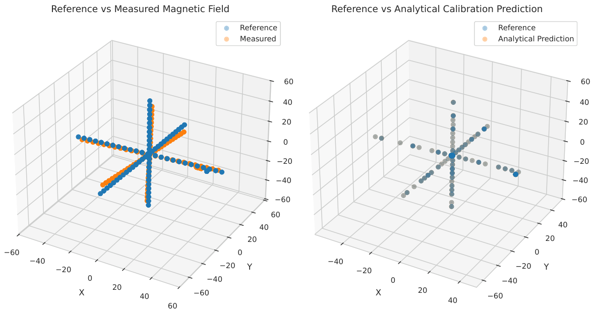
The three-dimensional scatter plots presented in Figure 1(left) indicate the deviation of the uncalibrated sensor readings from the reference magnetic field measurements, while Figure 1(right) shows the calibrated outputs obtained using the physics-based regression model. Although the calibrated measurements show significantly improved alignment with the reference field, noticeable dispersion persists, particularly along the Y-axis, indicating limitations of the standalone analytical model in fully compensating higher-order nonlinearities.

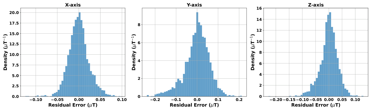
The residual histograms in Figure 2 indicate that the analytical model is unbiased across all axes, with distributions centered close to zero and roughly bell-shaped, showing good baseline calibration; the X-axis performs best with the smallest spread and minimal tails, suggesting mostly noise-level errors, while the Z axis shows moderate spread with slight asymmetry, pointing to minor systematic or nonlinear effects, and the Y-axis shows the largest variance and slightly heavier tails than the X- and Y-axes, implying unmodeled behavior such as stronger temperature coupling, cross-axis effects, or higher sensor noise—overall, the residuals are structured and learnable, making them well suited for further correction via a residual-learning neural network.

3.6. Hyperparameter Optimization and Model Selection for Residual Learning

To model the residual errors remaining after the physics-based calibration stage, the neural network architecture and training configuration were determined through a structured grid search comprising 960 hyperparameter combinations. The explored architectural ranges included 3–7 hidden layers and 32, 64, or 128 neurons per layer. DropConnect regularization rates of 0.005, 0.01, 0.1, and 0.2 were evaluated to control overfitting while preserving uncertainty estimation capability.

Optimization hyperparameters included learning rates of $1\times {10}^{-3}$ and $5\times {10}^{-4}$, batch sizes of 16 and 32, and training durations of 500, 1000, 1500, and 2000 epochs. All networks employed ReLU activation functions and an output layer with two neurons to predict the residual mean and log-variance, enabling heteroscedastic uncertainty modeling. Training was performed using the Adam optimizer with a custom negative log-likelihood loss function, incorporating log-variance clipping ($-10$ to 3) and variance regularization with a weight of ${10}^{-4}$.

A 90%/10% training–validation split was used for model selection. The optimal residual model consisted of four hidden layers with 64 neurons per layer, a DropConnect rate of 0.01, a learning rate of $5\times {10}^{-4}$, batch size of 16, and 1000 training epochs. This configuration achieved the lowest validation negative log-likelihood while maintaining stable RMSE performance and was therefore used for all reported hybrid calibration results.

To ensure stable convergence and prevent overfitting, an early stopping criterion based on validation loss was employed. Training was terminated when the validation loss failed to improve by at least ${10}^{-6}$ for 50 consecutive epochs, and the model weights corresponding to the minimum validation loss were restored. This stopping rule guarantees convergence of the gradient-based optimization while maintaining generalization performance.

3.7. Calibration Results for the Proposed Hybrid Framework

To address the residual nonlinearities and unmodeled effects observed after regression-based calibration, the proposed framework integrates the physics-based model with an HNN that learns the errors between the reference magnetic fields and the analytical predictions. The neural networks estimate both the residual mean and input-dependent aleatoric uncertainty, while epistemic uncertainty is estimated using MCDC during inference. Physics-based uncertainty is modeled independently. Aleatoric uncertainty is propagated through the analytical calibration model using the QMC sampling approach. Epistemic uncertainty due to parameter estimation is quantified using a combination of a Jacobian-based covariance approach and parameter posterior sampling propagation.

Table 7. Predictive performance metrics for the proposed hybrid framework under different likelihood models.

Likelihood	Axis	RMSE	MAE	Coverage (%)	NLL	CRPS
Laplace	X-axis	0.01624	0.01219	100.0	−1.230	0.02798
	Y-axis	0.03449	0.01654	100.0	−1.275	0.03002
	Z-axis	0.02080	0.01527	100.0	−1.251	0.02812
Student-t	X-axis	0.01624	0.01219	100.0	−1.230	0.02798
	Y-axis	0.03449	0.01654	100.0	−1.275	0.03002
	Z-axis	0.02080	0.01527	100.0	−1.251	0.02812
Heteroscedastic Gaussian	X-axis	0.01622	0.01226	98.52	−2.699	0.00891
	Y-axis	0.03459	0.01614	97.63	−2.732	0.01213
	Z-axis	0.02067	0.01482	98.52	−2.493	0.01069

presents the final performance of the proposed hybrid approach. Compared to the analytical calibration results reported in Table 5 and Table 6, the hybrid approach yields consistent reductions in both MAE and RMSE across all three axes. The most notable improvement is observed along the Y-axis, which previously exhibited the largest residual errors due to strong scale-factor mismatch and cross-axis coupling. Along with improved accuracy, the proposed hybrid approach delivers well-calibrated uncertainty estimates. The empirical coverage of the predicted confidence intervals exceeds 95% for all axes, as reported in Table 7, indicating statistically reliable uncertainty estimations.

Table 8. X-axis predictions and uncertainty decomposition using the hybrid calibration framework.

Index	Actual	Measured	Predicted	Aleatoric_Physics	Epistemic_Physics	Aleatoric_NN	Epistemic_NN	Total_Uncertainty	Lower_Bound	Upper_Bound	Coverage
0	43.9477	37.4288	43.9384	0.0119	0.0016	0.0140	0.0042	0.0189	43.9014	43.9754	True
1	−0.0033	0.3243	−0.0006	0.0110	0.0005	0.0136	0.0015	0.0176	−0.0352	0.0339	True
2	4.7700	4.7040	4.7781	0.0111	0.0005	0.0163	0.0030	0.0199	4.7390	4.8171	True
3	43.9436	37.3532	43.9509	0.0119	0.0015	0.0131	0.0048	0.0184	43.9149	43.9870	True
…
334	0.4290	0.7225	0.4294	0.0110	0.0005	0.0158	0.0014	0.0193	0.3915	0.4673	True
335	43.9343	35.9532	43.9026	0.0124	0.0022	0.0181	0.0047	0.0225	43.8584	43.9468	True
336	43.9410	36.1624	43.8907	0.0123	0.0018	0.0169	0.0027	0.0211	43.8493	43.9320	False
337	0.3855	0.7950	0.3994	0.0111	0.0008	0.0117	0.0032	0.0165	0.3671	0.4317	True

,

Table 9. Y-axis predictions and uncertainty decomposition using the hybrid calibration framework.

Index	Actual	Measured	Predicted	Aleatoric_Physics	Epistemic_Physics	Aleatoric_NN	Epistemic_NN	Total_Uncertainty	Lower_Bound	Upper_Bound	Coverage
0	−1.3932	2.2641	−1.3935	0.0014	0.0040	0.0054	0.0035	0.0077	−1.4086	−1.3783	True
1	0.3970	0.4221	0.3886	0.0114	0.0013	0.0063	0.0026	0.0133	0.3625	0.4146	True
2	0.7775	1.1942	0.7895	0.0113	0.0013	0.0122	0.0067	0.0180	0.7542	0.8247	True
3	−1.3954	2.2667	−1.3986	0.0012	0.0039	0.0057	0.0032	0.0077	−1.4136	−1.3835	True
…
334	0.5800	0.5767	0.5702	0.0113	0.0012	0.0161	0.0069	0.0208	0.5294	0.6111	True
335	−1.4090	1.9344	−1.4037	0.0049	0.0056	0.0091	0.0105	0.0157	−1.4345	−1.3729	True
336	−1.4090	1.9751	−1.3994	0.0040	0.0046	0.0066	0.0060	0.0108	−1.4206	−1.3782	True
337	0.5160	0.7916	0.5249	0.0111	0.0020	0.0113	0.0086	0.0181	0.4893	0.5604	True

and

Table 10. Z-axis predictions and uncertainty decomposition using the hybrid calibration framework.

Index	Actual	Measured	Predicted	Aleatoric_Physics	Epistemic_Physics	Aleatoric_NN	Epistemic_NN	Total_Uncertainty	Lower_Bound	Upper_Bound	Coverage
0	0.8716	−0.8316	0.8718	0.0105	0.0022	0.0113	0.0036	0.0160	0.8404	0.9032	True
1	−0.1237	−0.6149	−0.1492	0.0113	0.0007	0.0146	0.0027	0.0187	−0.1858	−0.1126	True
2	0.1789	−0.4496	0.1489	0.0113	0.0007	0.0192	0.0073	0.0234	0.1031	0.1948	True
3	0.9147	−0.7760	0.9324	0.0105	0.0021	0.0137	0.0029	0.0176	0.8979	0.9669	True
…
334	−0.1485	−0.6202	−0.1441	0.0113	0.0007	0.0140	0.0036	0.0184	−0.1801	−0.1081	True
335	0.8449	−0.7668	0.8419	0.0101	0.0031	0.0147	0.0036	0.0185	0.8058	0.8781	True
336	0.8759	−0.7819	0.8547	0.0102	0.0026	0.0127	0.0019	0.0166	0.8221	0.8872	True
337	9.2325	7.8901	9.2548	0.0114	0.0011	0.0604	0.0084	0.0620	9.1333	9.3764	True

demonstrate that the hybrid calibration approach adequately corrects substantial measurement bias while providing well-structured and well-calibrated uncertainty estimates. In all three axes, the measured magnetic fields often deviate notably from the reference values, whereas the predicted values are consistently very close to the reference magnetic field values, signifying that the proposed hybrid framework effectively compensates for systematic sensor errors. The uncertainty breakdown exhibits a stable contribution from the physics-based aleatoric component, suggesting that inherent physical noise is well characterized, while the neural network contributes more variability. This demonstrates that most of the remaining predictive uncertainty arises from the learned correction rather than the underlying physical model. The total uncertainty values produce tight confidence intervals, and coverage is almost always true, exhibiting effective calibration with only rare slight under-coverage. Particularly in more challenging cases—such as larger-magnitude values in the Z-axis—the model adequately increases neural network aleatoric uncertainty, resulting in wider confidence intervals while still maintaining correct coverage. Overall, the results validate that the hybrid framework achieves high predictive accuracy, effective bias correction, meaningful uncertainty decomposition, and reliable confidence interval calibration across all three axes.

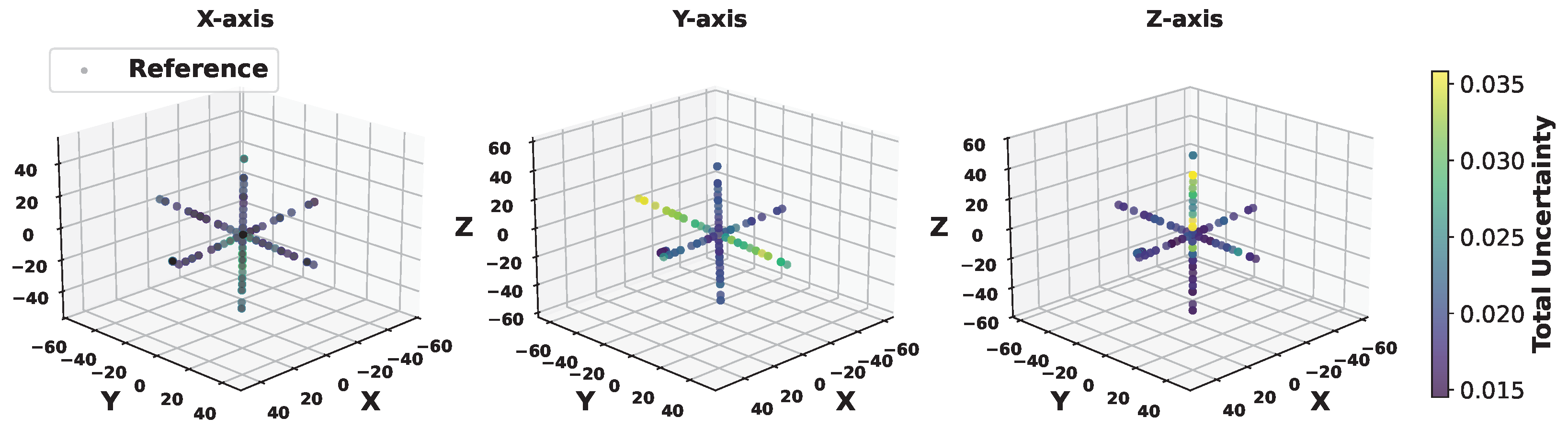
Figure 3 shows the alignment between predicted and reference magnetic field components for the X, Y, and Z axes, with color illustrating the overall predictive uncertainty. The X-axis shows close geometric agreement and low uncertainty, indicating that dominant error sources are effectively characterized by the physics-based model. On the other hand, the Y-axis exhibits increased dispersion and prominent uncertainty, consistent with its larger RMSE and the presence of scale-factor mismatch and cross-axis coupling. The Z-axis characterizes intermediate behavior with moderate uncertainty and good alignment, suggesting predominantly systematic errors. Overall, the results confirm strong axis-dependent calibration performance, with the Y-axis contributing most significantly to the residual error budget.

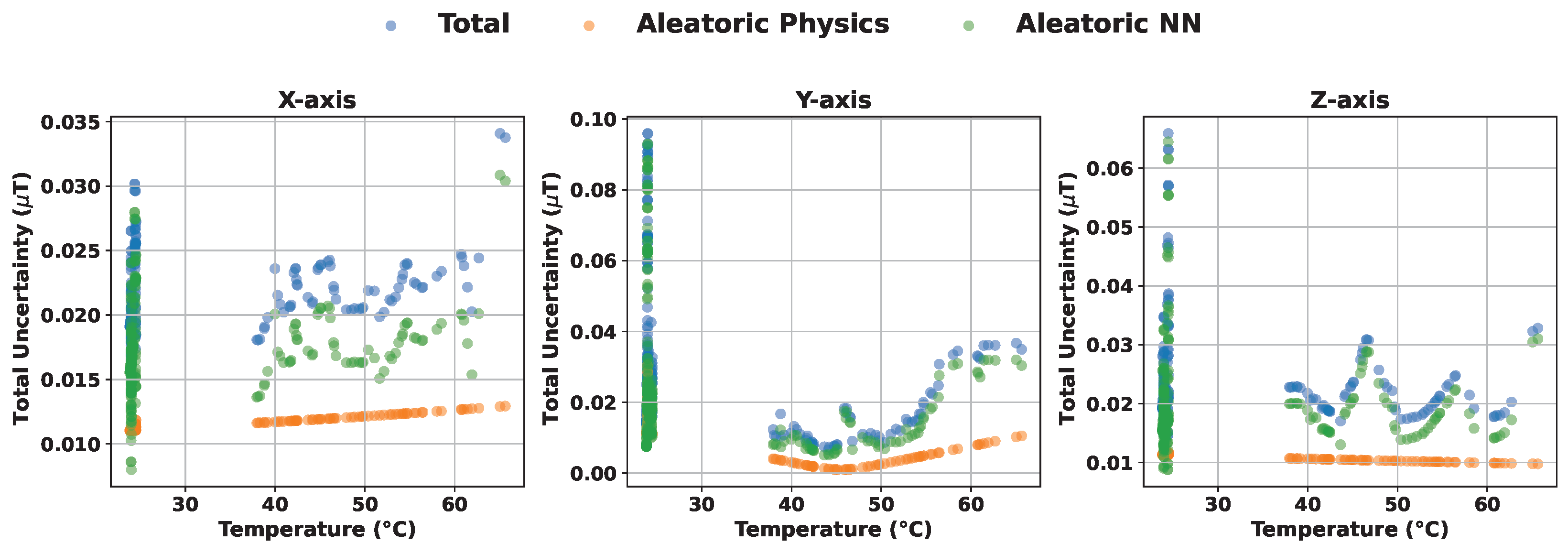
Figure 4 illustrates the temperature-dependent uncertainty partitioning along the X-, Y-, and Z-axes, decomposing the total predictive uncertainty into the aleatoric contributions from the physics-based model and the neural network (NN). For the X-axis, the physics-based component is small and nearly constant, indicating low intrinsic noise in the analytical model. In contrast, the NN aleatoric uncertainty is slightly larger and temperature-dependent, contributing more substantially to the total uncertainty, particularly at higher temperatures. Along the Y-axis, the total uncertainty is generally higher, especially at low temperatures, with the NN uncertainty dominating. Above 55 °C, the NN captures most of the variability, suggesting that the hybrid model experiences greater difficulty in accurately predicting Y-axis behavior in the high-temperature range. For the Z-axis, the total uncertainty exhibits the largest variation across temperatures. The physics-based contribution remains low and nearly flat, whereas the NN contribution shows pronounced temperature-dependent peaks. This indicates that Z-axis predictions are the most challenging, with NN-corrected residuals introducing substantial variability, likely due to less accurate calibration in specific regions.

At low temperatures, regions of nearly constant temperature exhibit substantial variability in predictive uncertainty. This behavior arises because the uncertainty is not solely a function of temperature but depends on the full input vector $\mathbf{x}=(B_x,B_y,B_z,T).$ Even when temperature remains approximately constant, variations in magnetic field magnitude and direction alter the sensitivity of the calibration model and the neural network residual predictor. In particular, cross-axis coupling terms and nonlinear scale-factor effects introduce input-dependent variance amplification. Consequently, the observed spread in uncertainty at low temperatures reflects input-dependent sensitivity rather than temperature variation alone.

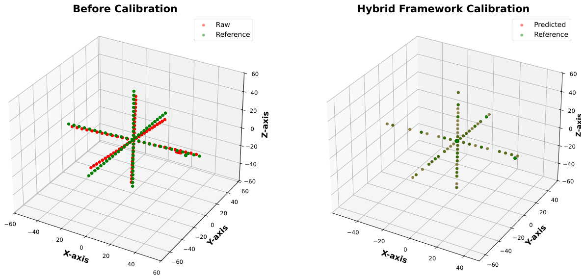
Figure 5 highlights the 3-dimensional distribution of magnetic field values before and after applying the hybrid calibration framework, comparing it with the reference values. Before calibration, the measured magnetic values show substantial discrepancies and distortions relative to the reference, indicating the presence of systematic errors. After hybrid calibration, the measurements indicate significantly improved alignment with the reference values, showing reduced dispersion and enhanced accuracy. This indicates the performance of the proposed hybrid calibration approach in compensating for measurement errors and improving magnetic field estimation.

3.8. Comparative Analysis of Likelihood Models

Table 7 presents a comparative evaluation of the Laplace, Student-t, and heteroscedastic Gaussian likelihood formulations using proper scoring rules and calibration-based metrics. Lower RMSE, MAE, NLL, and Continuous Ranked Probability Score (CRPS) values indicate improved predictive accuracy and sharper probabilistic forecasts.

All three models exhibit comparable deterministic accuracy in terms of RMSE and MAE. However, the heteroscedastic Gaussian formulation achieves substantially lower NLL and CRPS values, indicating sharper and more informative predictive distributions with empirical coverage close to the nominal 95% level. In contrast, the Laplace and Student-t likelihoods yield over-dispersed predictive intervals with 100% empirical coverage, suggesting conservative uncertainty quantification. These findings imply that, following physics-based error correction, the residual error distribution is well-approximated by a Gaussian model.

3.9. Discussion

The data analysis results reveal that physics-based calibration provides a strong and physically interpretable baseline but is inadequate to fully capture the complex nonlinear and temperature-dependent effects inherent in AMR sensors. The proposed hybrid approach successfully bridges this gap by integrating analytical modeling with probabilistic deep learning, resulting in both enhanced calibration performance and statistically consistent uncertainty quantifications. The quantitative improvements reported in Table 5 and Table 6, together with the visual comparisons in Figure 1 and Figure 5, emphasize the benefits of explicitly separating physics-based and data-driven uncertainty sources. These properties are particularly important for safety-critical and high-reliability applications, where both accuracy and trustworthy uncertainty quantification are crucial.

3.10. Limitations and Future Work

Despite its demonstrated effectiveness, the proposed hybrid framework has several limitations. First, the experimental benchmarking is constrained to a controlled laboratory dataset with static magnetic fields and regulated temperature variations. Real-world operating environments may introduce additional sources of uncertainty, including time-varying magnetic disturbances, mechanical stress, sensor aging, and environmental factors, in addition to thermal effects. Second, the physics-based model assumes linear temperature dependence of calibration parameters, which may not fully capture higher-order thermal effects under challenging operating conditions.

Future study will focus on enhancing the hybrid framework to dynamic and in-situ calibration conditions involving time-varying magnetic fields and long-term sensor drift. Including additional environmental variables, such as humidity and pressure, into the physics-based model will be investigated to further enhance system reliability. Finally, the proposed framework will be tested across different AMR sensor models and alternative magnetometer technologies to assess its generalizability and scalability.

3.11. Computational Performance of the Hybrid Calibration Framework

The proposed hybrid framework used for primary validation (500 parameter samples, 1000 Sobol Quasi-Monte Carlo samples, and 1000 training epochs) was conservatively formulated to verify statistically stable uncertainty quantification and robust benchmarking. Under this setting, the per-sample inference time for full three-axis calibration was approximately 0.12 s (

Table 11. Computational cost comparison (time in seconds).

Metric (s)	Validation	Reduced
	(500 Param, 1000 QMC, 1000 Epochs)	(100 Param, 500 QMC, 500 Epochs)
Total training time (3 axes)	505.50	250.74
Total inference time (3 axes)	39.47	18.65
Per-sample training time	0.166	0.082
Per-sample inference time	0.117	0.055
Physics model fitting time	0.165	0.011

).

To assess practical deployment feasibility, a reduced configuration consisting of 100 parameter samples, 500 QMC samples, and 500 training epochs was further analyzed. In this configuration, the total training time for the three-axis model was reduced to 251 s, while the total inference time for 338 test samples decreased to 18.65 s. This corresponds to a per-sample inference time of approximately 0.055 s (Table 11).

This represents an approximate 53% reduction in inference time while maintaining the same modeling structure and hybrid formulation. The observed behavior demonstrates that computational cost scales approximately linearly with the number of parameter samples ($N_q$) and QMC samples ($N_p$). Since the major computational demand arises from repeated stochastic sampling for uncertainty propagation, reducing the number of iterations directly lowers inference latency without requiring architectural modifications. These results show that the proposed hybrid framework is computationally flexible and can be systematically tuned to satisfy application-specific latency and deployment constraints, including near-real-time operation scenarios.

4. Simulation Study

4.1. Theoretical Formulation

To rigorously evaluate the proposed hybrid calibration framework, a controlled Monte Carlo simulation study was conducted to assess calibration accuracy, scalability, and robustness under known physical conditions while ensuring full traceability of the ground truth. A synthetic three-axis anisotropic magnetoresistive (AMR) sensor was simulated using the previously defined temperature-dependent affine calibration model, with physically consistent sensitivity, cross-axis coupling, and offset parameters.

For simulation purposes, the analytical model was inverted to generate raw sensor measurements from known reference magnetic fields, thereby ensuring that the true calibration parameters were exactly known and enabling unbiased performance evaluation. The inversion used to synthesize measurements is expressed as

$${\mathbf{B}}_{\mathrm{meas}}={\left(\mathbf{S}+{\mathbf{K}}_{s}T\right)}^{-1}\left({\mathbf{B}}_{\mathrm{ref}}-\mathbf{O}-{\mathbf{K}}_{o}T\right).$$

(43)

This formulation guarantees mathematical consistency, since deviations between predicted and reference values arise solely from estimation error and imposed distortions. To emulate realistic AMR sensor behavior, additive Gaussian measurement noise with a standard deviation of 0.5 µT was incorporated into the simulated measurements.

In addition, a structured nonlinear distortion was introduced into the Y-axis measurement according to

$$B_{y,\mathrm{meas}}\leftarrow B_{y,\mathrm{meas}}+0.01B_{x,\mathrm{meas}}^2,$$

(44)

thereby generating residual behavior that cannot be captured by the linear thermo-affine calibration model and providing a meaningful validation scenario for the proposed correction strategy.

Such a quadratic nonlinear distortion can arise in practical AMR sensors due to several physical mechanisms. First, imperfect magnetic shielding and sensor bridge asymmetry may produce cross-axis coupling, where the magnetic field component along one axis influences the response of another axis in a nonlinear manner. Second, AMR sensors can exhibit weak magnetic hysteresis and partial saturation effects when exposed to varying magnetic field magnitudes, which may introduce higher-order nonlinear terms beyond the linear thermo-affine model [1,2]. The quadratic term introduced in the Y-axis therefore serves as a simplified representation of these higher-order cross-axis and nonlinear sensor effects, allowing the simulation to evaluate whether the proposed framework can effectively compensate for realistic residual nonlinearities that are not captured by the analytical calibration model.

4.2. Experimental Design and Dataset Generation

To assess scalability and convergence, synthetic datasets containing 50,000, 100,000, 200,000, and 500,000 observations were generated. The true magnetic field components were uniformly sampled within $\pm 50$ µT, and temperature was uniformly sampled between 0 °C and 40 °C. The same physical parameter set was used in all experiments to ensure strict comparability.

Each dataset was randomly divided into training and testing subsets using an 80–20 split. The physics-based calibration parameters were estimated from the training data via nonlinear least squares. Subsequently, the heteroscedastic neural network was trained to learn the residual error between the physics-based prediction and the reference field. Performance evaluation was conducted exclusively on the independent test subset to ensure unbiased assessment.

4.3. Performance Evaluation

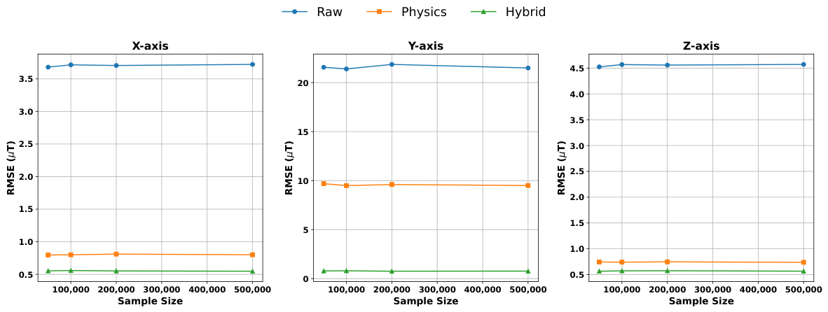
The simulation results consistently demonstrate substantial performance improvements when moving from raw measurements to physics-based calibration, and further improvement when applying the hybrid model. For example, at a sample size of 50,000 observations, the raw Y-axis RMSE exceeded 21 µT, reflecting strong cross-axis coupling and nonlinear distortion in the simulated sensor. Physics-based calibration reduced this error to approximately 9.7 µT, indicating successful compensation of linear thermo-affine effects. The proposed hybrid model further reduced the RMSE to approximately 0.78 µT, approaching the intrinsic noise level of the sensor (

Table 12. RMSE comparison across sample sizes (test data only).

Sample Size	Axis	RMSE Raw	RMSE Physics	RMSE Hybrid
50,000	X	3.6807	0.7971	0.5532
	Y	21.5638	9.6876	0.7847
	Z	4.5241	0.7448	0.5657
100,000	X	3.7163	0.8002	0.5588
	Y	21.3935	9.4931	0.7975
	Z	4.5685	0.7415	0.5729
200,000	X	3.7061	0.8108	0.5522
	Y	21.8569	9.6005	0.7551
	Z	4.5585	0.7473	0.5746
500,000	X	3.7228	0.8009	0.5477
	Y	21.4943	9.5040	0.7694
	Z	4.5719	0.7376	0.5669

).

Similar behavior was observed for the X- and Z-axes, where the hybrid model consistently reduced residual error beyond the physics-only solution. Increasing the sample size from 50,000 to 500,000 did not produce significant changes in RMSE values. The raw measurement error remained constant, as expected, since intrinsic sensor distortion is independent of dataset size. The physics-based RMSE stabilized rapidly, indicating parameter convergence. The hybrid model also exhibited stable performance across all dataset sizes, demonstrating effective generalization without overfitting (Figure 6).

The large reduction in Y-axis error highlights the hybrid model’s ability to capture nonlinear distortions not represented in the analytical calibration equation. Since the nonlinear term was deliberately introduced into the simulation, this result provides strong evidence that the hybrid framework compensates for higher-order residual effects while preserving physical interpretability.

4.4. Statistical Significance of Hybrid Improvement

Let $e_{\mathrm{phys}}$ and $e_{\mathrm{hyb}}$ denote the prediction errors of the physics-based and hybrid models respectively. The null hypothesis was formulated as

$$H_0:\mathbb{E}\left[e_{\mathrm{phys}}^2-e_{\mathrm{hyb}}^2\right]=0,$$

(45)

while the one-sided alternative hypothesis assumed

$$H_1:\mathbb{E}\left[e_{\mathrm{phys}}^2-e_{\mathrm{hyb}}^2\right]>0,$$

(46)

indicating superior performance of the hybrid model.

The paired squared-error analysis conducted on the independent test set for $N=100,000$ demonstrated statistically significant improvement across all three axes. For the X-axis, the mean reduction in squared error was 0.332 µT² with a t-statistic of 44.29 and $p<{10}^{-15}$; the 95% confidence interval (0.317 to 0.346 µT²) and Cohen’s $d=0.44$ indicate a moderate practical effect. For the Y-axis, the mean reduction was 89.43 µT² with a t-statistic of 52.78 and $p<{10}^{-15}$; the corresponding confidence interval (86.11 to 92.75 µT²) and Cohen’s $d=0.53$ confirm a robust and practically meaningful improvement. For the Z-axis, the mean reduction was 0.221 µT² with a t-statistic of 65.58 and $p<{10}^{-15}$; the confidence interval (0.215 to 0.228 µT²) and Cohen’s $d=0.66$ indicate a large and stable effect (

Table 13. Statistical Significance analysis of hybrid vs. physics-based calibration (N = 100,000).

Axis	Mean Diff.	t-Statistic	p-Value	95% CI Lower	95% CI Upper	Cohen’s d
X-axis	0.3317	44.2946	<0.001	0.3170	0.3464	0.4429
Y-axis	89.4303	52.7799	<0.001	86.1089	92.7517	0.5278
Z-axis	0.2212	65.5799	<0.001	0.2146	0.2279	0.6558

).

Overall, the null hypothesis of equal expected squared error is decisively rejected. The same paired squared-error procedure applied to $N=50,000$, 200,000, and 500,000 yielded strictly positive mean reductions and highly significant results ($p<0.001$) for all axes, confirming statistical robustness and scalability.

4.5. Interpretation

From a metrological context, the simulation study validates three fundamental properties of the proposed hybrid framework. First, the hybrid framework yields significant bias reduction beyond traditional curve fitting. Second, physical interpretability is retained because the neural network operates only on residual errors rather than replacing the analytical model. Third, the approach validates scalability and statistical stability over large datasets, indicating suitability for industrial and high-precision metrological applications. Overall, the results demonstrate the theoretical premise that combining physically interpretable calibration with data-driven residual modeling yields superior accuracy compared to either approach alone. The hybrid framework adequately compensates nonlinear distortions while maintaining traceability to physical calibration parameters.

5. Conclusions

This study proposed a hybrid physics-based and data-driven calibration approach for AMR sensors with explicit and well-calibrated uncertainty quantification. The proposed framework combines a temperature-compensated analytical calibration model with a probabilistic neural network–based residual correction, thereby retaining physical interpretability while improving modeling adaptability. The physics-based model specifically accounts for scale-factor errors, cross-axis coupling, offsets, and temperature-dependent effects, whereas the data-driven approach captures residual nonlinearities.

The proposed framework was examined using a secondary dataset derived from controlled Helmholtz-coil experiments on a commercial HMC1053 AMR sensor [2]. Experimental results exhibit that while standalone physics-based calibration substantially reduces systematic errors relative to raw measurements, residual axis-dependent errors—most prominently along the Y-axis—persist due to complex temperature-dependent behavior. The proposed hybrid framework successfully reduces these errors, achieving lower RMSE and MAE across all axes while retaining strong agreement with reference magnetic fields.

A key contribution of this study is its rigorous and transparent uncertainty quantification. Aleatoric uncertainty is propagated through the physics-based model using the QMC sampling approach, while epistemic uncertainty is estimated via an integration of Jacobian-based covariance propagation and the parameter posterior sampling approach. The neural network component further models input-dependent aleatoric uncertainty and epistemic uncertainty through HNNs and MCDC. The integration of physics-based and data-driven uncertainty sources yields statistically consistent confidence intervals with empirical coverage exceeding 99%, validating the reliability of the proposed uncertainty estimates.

Overall, the proposed approach provides a physically interpretable, uncertainty-aware, and robust calibration solution for AMR sensors operating under varying thermal conditions. The framework is well suited for high-reliability applications in geomagnetic monitoring, navigation, and space instrumentation, where both accuracy and trustworthy uncertainty estimates are crucial.