


Abstract
Ceramic-matrix-composite (CMC) turbine seal segments lose their gas-side coatings in service. Assessing one loss configuration takes a thermal and a mechanical finite-element solve, and there are too many admissible configurations to solve them all. A surrogate makes it affordable and follows it as the loss progresses. We build one on 5452 solves of a published seal-segment model with coating added, specify its toolchain in full, and compare four digital-twin techniques: a neural network against reduced-basis and full-field Gaussian processes. Swapping a lost cell to a higher-conductivity material instead of deleting it costs about 1 °C in the mean but 100 °C at the rim, an error that stays on the sacrificial coating and under-reads the substrate by at most 11.5 °C. That error is one-signed: a bias to be carried, not a scatter. On a reduced basis the basis binds, not the regressor: neither model improves with data. Restricting the design to the service-marked loss zones is worth on one layer and to on two. The recommended full-field twin returns the peak coating-interface temperature within 0.23 °C at 3 ms per pattern, but a free superposition baseline beats it in the maintenance regime.
1. Introduction
A high-pressure turbine seal segment is the stationary shroud that surrounds the rotor and sets the blade-tip clearance [1]. Ceramic-matrix composites have entered service for this component because they operate a few hundred degrees above nickel superalloys at about one third of the weight. The CFM International LEAP engine carries eighteen SiC/SiC first-stage high-pressure-turbine shrouds rated to C at the coating interface [2], and Rolls-Royce has demonstrated CMCs in the UltraFan high-pressure turbine, primarily as seal segments [1]. The substrate is protected on its gas-side face by an abradable coating over an environmental barrier coating. The progressive loss of these coatings in service raises the local substrate temperature and steepens the thermal gradient, which drives the thermal stress responsible for crack initiation [3,4].
Assessing that risk means evaluating many loss patterns, and each pattern costs a thermal and a mechanical finite-element solve. No analyst can run that pair for every admissible configuration: the two-layer model of this paper admits of them, and one solve takes nineteen minutes. The building blocks are established in the literature: reduced-basis emulation of high-dimensional field outputs [5,6,7], and graph-based and residual variants [8,9]. That literature leaves open which of the assumptions underneath such a surrogate actually bind on a damage-configuration problem of this kind. Three are open: whether the model simplification that makes a campaign affordable is admissible, whether a truncated basis limits the attainable error, and where the training points should be placed. The cost is not the whole of it. A surrogate that answers in milliseconds also lets the analyst follow the component state by state as the coating is progressively lost, instead of at a handful of configurations chosen in advance. This is how the damage accumulates in service. The twin supplies the field at every state, and the analyst supplies the damage law.
What we deliver is that toolchain: the generation of the finite-element decks, the design of experiments, the four surrogates, the uncertainty estimate and a self-contained predictor that needs no solver, specified here in the detail a reader needs to rebuild it. Nothing in it is specific to this component, so it carries over to any problem in which a field must be predicted from a discrete damage or configuration state. The second contribution is the comparison of the digital-twin techniques on the same data, and with it the measurement of the three assumptions above, which decide whether the surrogate is worth building at all.
1.1. Our Results
On 5452 finite-element solves of an engine-grade CMC seal-segment model (284,745 nodes, a grid of coating cells), we quantify the three assumptions that a coating-loss surrogate rests on and report a fourth result that emerged from the comparison.
- The simplification that makes such a campaign affordable has two regimes that must be reported together. Replacing a lost cell by a higher-conductivity material rather than deleting its elements (Section 4.1) is sound in the mean, below C up to four lost cells and C at six, but wrong by C on the rim of the lost patch. That error stays on the sacrificial coating and reaches the CMC substrate by at most C, one-signed and non-conservative.
- On a reduced basis the binding constraint is neither the data nor the regressor: at twenty modes a Gaussian process and a neural network reach the same error, and neither improves with data (Section 4.2). An exact full-field Gaussian process, made tractable by the separable multi-output structure [10,11], truncates nothing and is the most accurate of the four. On the two-layer problem, it alone profits from more data (Section 4.7).
- Where the training points are placed is worth more than how many there are. Restricting the design of experiments to the zones where coating is actually lost buys a factor of on one layer and to on two, at equal cost, for a zone drawn from the service marks (Section 4.6). Error is governed by distance from the design, so a uniformly trained surrogate is worst in the very maintenance regime it is meant to serve.
- The free physical baseline is the real competitor of a machine-learned surrogate. In the loss regime in which maintenance operates, the twin leads in norm and on the mean interface temperature and the gradient. But a free linear superposition of single-cell responses beats it by a factor of about thirty on the peak interface temperature, the one quantity a designer reads (Section 4.5).
The recommended twin returns that peak within C at 3 ms per pattern in batched use and knows when it is out of its design (Section 4.4). Applied to the cracks of the reference study, it shows that neither grows without limit: one is never driven at all, and the other advances and arrests at every discretisation run. A crack seeded at the true trailing-edge stress maximum grows and is not lengthened by coating loss (Section 4.8 and Section 4.9). A companion paper treats the inverse problem, recovering the loss state from sparse sensors with sensor placement and remaining-useful-life estimation.
1.2. A Reader’s Guide to This Paper
The recommendation of this paper is a full-field Gaussian process: fitted to the whole temperature field, it is the twin we would deploy, and Section 4.3 establishes it. Four statements carry the rest, and a reader in a hurry can find each in one place.
- The simplification under-reads the substrate in one direction (Section 4.1). A designer using it for margin assessment must carry that as a bias, not a scatter: the under-prediction on the substrate face peak grows to C at total loss.
- The reduced-basis twins saturate because the basis binds, not the regressor (Section 4.2). Once the held-out error sits on the projection error of the basis, further simulations buy nothing, and the budget must go into the basis or into a method that truncates none.
- In the maintenance regime, a free linear superposition beats the trained twin (Section 4.5) by about a factor of thirty, at no training cost, being exact while the lost cells stay isolated and inexact once they cluster.
- Where the simulations are spent matters more than how many (Section 4.6), and most of all through the definition of the zone they are concentrated in; the sensitivity the recommendation is conditional on.
Section 4.8 and Section 4.9 are a separate strand: they read the twin’s fields through a fracture criterion, and they bound what this model may and may not be asked. Section 4.10 presents the limitations.
2. Problem Formulation
Let the gas-side face of the seal segment be discretised into cells, each carrying a coating coverage (denoted intact for and lost for ). The steady substrate temperature T obeys an energy balance with lateral conduction, a prescribed gas-side heat flux, film and radiation exchange on the back cavity and on the top and side surfaces, and the through-thickness conduction resistance of the coating stack [12,13].
The gas path enters as an imposed flux, not as a convective exchange: losing a cell’s coating does not change the heat entering the component. It removes a resistance in series ahead of the substrate. The map from the coverage field to T is therefore nonlinear only through radiation and through the lateral conduction that couples neighbouring cells, and it is close to linear in the loss pattern. The near-linearity is a property of this load case rather than of the component. Any conclusion drawn from it holds for a flux-driven condition and would have to be re-established under a convective one, where losing coating also raises the local heat input. That caveat is about the driving temperature, and not about the geometry the loss opens: the step a lost cell leaves is bounded in Section S5 of the Supplementary Materials, and the length over which the surface state is smoothed is presented in Section 3.1.
The failure-critical part is the CMC substrate rather than the coating, which is sacrificial: the blade tip removes the abradable in service by design, and the barrier layer is there to be consumed. Accordingly, every error in this paper is reported both over the whole model and on the substrate alone, and acceptability is judged against the substrate value. The design quantities themselves are read one interface higher, on the surface between the abradable and the barrier, which is the hot surface the loss acts on directly. The substrate follows it mm below, its peak C colder on the intact component, and no pattern we solved moves that peak by more than three degrees (Section 4.3).
The reason a designer cares is that losing coating over a cell presents five risks at once:
- The gas-side surface runs hotter over the lost cells, and the substrate below it has a service limit that the assessment has to check.
- The thermal gradient steepens, which raises the thermal stress and with it the risk of cracking.
- The barrier layer no longer shields the substrate from the gas path, which raises the risk of recession.
- The substrate is exposed to water vapour and oxygen, which raises the risk of oxidation, whose coupling with stiffness degradation in this material system is modelled in [14].
- The seal segment stands further from the blade tip, since the lost coating set that clearance [1]. The tip leakage grows, the stage loses efficiency, and the gas-path condition the segment sees is no longer the one it was assessed under.
Only the first two are computed in this work. The others bound the interpretation of the results, and the authors regard the last, the opening of the tip clearance, as the principal limitation of this study (Section 5). Figure 1 shows what one such loss does to the component: the pattern, the temperature field it produces, and the in-plane gradient that carries the thermal stress.
Figure 1.
A coating-loss pattern of five lost cells (dashed outlines), the temperature field the engine-grade finite-element model produces from it, and the magnitude of the in-plane gradient, both read on the coating interface. The temperature rises over the lost cells; the gradient is dominated by the component edges, not by the patch, which is why coating loss moves the peak thermal stress so little (Section 4.8).
3. Materials and Methods
3.1. The Finite-Element Model
The model used throughout is the seal-segment model of [13], to which the coating system was added. Nothing in it is proprietary. The geometry, the material data and the thermal boundary conditions are those published there. The coating layers are the subject of this work, and the finite-element input files (the decks, in the following section) are part of the material deposited on acceptance (Section 3.6).
The component is the seal-segment-like structure of [13], inspired by the GE Aviation geometry in service. It is a curved plate carrying four pin-holder protrusions, spanning 60 mm axially, 77 mm circumferentially and 29 mm radially, with the coating footprint covering mm of the gas-side face (Figure 2). The mesh differs from that of [13], which meshed the uncoated substrate with 355,419 quadratic HEX20 elements and 1,545,569 nodes. The deck used here carries the three coating layers and the cell partition of Section 3.2 and is meshed with 259,096 linear elements (258,616 hexahedra and 480 wedges of type DC3D6) and 284,745 nodes. Of these, three belong to no element and are not reported by the solver, so every temperature field in this paper carries 284,742 values, the output dimension of the surrogates. The hexahedra are run at full integration, type DC3D8.
Figure 2.
The finite-element model of the seal segment: the curved plate, the four pin-holder protrusions and the mesh. The gas-side face is the underside of the plate and carries the coating system.
The deck as received declares the hexahedra reduced-integration C over the whole campaign, and every analysis reported here uses the substituted deck. Resolving coating layers of , and mm through the thickness of a component 29 mm thick demands elements far smaller than the substrate alone would require. At that refinement, quadratic interpolation would not support a campaign of thousands of solves, so the coated deck trades element order for element count. In the plan, the elements are about mm, five hundred to a coating cell in each element layer (400 in the narrower trailing-edge column). Five element layers resolve the mm coating stack: three across the abradable, one across the environmental barrier and one across the bond coat (Figure 3).
Figure 3.
Detail of the coating system at the trailing edge. From the substrate outwards: the CMC (pink), the bond coat BND ( mm, thin light layer), the environmental barrier coating EBC ( mm) and the abradable ABR ( mm, resolved by three element layers). The distinct colours on the gas-side face are the individual coating cells of the partition (Section 3.2); the grey wedge on the left is the deltoid filler.
The coating system has three layers, whose thicknesses we measured from the mesh rather than assumed. It comprises a bond coat (BND) of mm in a single element layer, an environmental barrier coating (EBC) of mm in a single element layer, and an abradable (ABR) of mm resolved by three element layers of mm each (Figure 3). Between the pin-holder protrusions the model carries two deltoid fillets, roughly triangular filler regions that support the joint and have no structural function. They are meshed as solid material and assigned their own material card (the block of the deck that defines a material), and Section 4.8 returns to the consequence of that choice.
Table 1 collects every material in the model. The orthotropic CMC substrate follows Table 1 of [13] and Table 1 of [15]. The three coating layers follow Tables 6–8 [16], matched property by property, density included. The deck carries the values used throughout and settles the matter where the published tables disagree: the transverse shear moduli of the substrate at C are 102,300 MPa, as in [15]. These follow the ratio by which the in-plane constants are reduced over that interval, which also follows at 141,174 MPa; the through-thickness modulus falls further, by , and the differing figures elsewhere are typographical. Only the deltoid card and the fictitious materials of Section 3.2 are specific to this deck. All properties are tabulated at 20 and C and interpolated linearly between them. Above C the solver extrapolates them as constant, which is a limitation of the model wherever the field exceeds that temperature.
Table 1.
Material data of the finite-element model, at 20 and C. The CMC substrate and deltoid filler are orthotropic: directional entries are separated by slashes, in the order 1, 2 in-plane, and 3 through-thickness; the coating layers (BND, EBC, ABR) carry one value per property. Units: k mW , t , E and G MPa, , .
Canale et al. [16] ran a three-level design of experiments over the three thicknesses. The values used here, mm (ABR), mm (EBC) and mm (BND), are the middle level of all three: the nominal configuration of that study, rather than the optimum it selected (, and mm). The present work therefore assesses coating loss on the nominal build, and the interaction between layer-thickness optimisation and loss tolerance is left open.
The deltoid is declared orthotropic in the deck exactly as the substrate is, through the same nine engineering constants and the same three directional constants for conductivity and expansion, but its constants coincide across the three directions. Its three directions therefore carry identical constants, and the card departs from a single-modulus one only by the that separates its shear modulus from (G = 121,440 against 120,000 MPa). We report it as the deck defines it. The deltoid card is not consistent with the deltoid’s stated function: the deck assigns this non-structural filler a stiffness of the same order as the substrate, 276,000 against 345,000 MPa, and a thermal expansion coefficient lower than the substrate’s. A stiff inclusion with a mismatched expansion coefficient concentrates thermal stress, and the largest reading of the free-expansion model falls on the deltoid fillets (Section 4.8)—at the one place where that model does not apply. The fillets are nevertheless excluded from the crack analysis, because in service the segment is mechanically fixed at them and a free-expansion model that applies no attachment load does not represent the stress there. Every error is reported with the fillets held apart from the substrate, and Section 4.8 explains why no stress reading on them is quoted anywhere in this work.
The thermal load is the nominal, uncooled condition of [13], with none of the nine impingement cooling jets active. A uniform heat flux is applied to the three gas-path zones of the gas-side face, and the component dissipates by convection and radiation through the top and side surfaces and through the back cavity. Table 2 gives the film and radiation data, those of Table 3 of [13], reproduced exactly by the deck, surface by surface. The applied gas-path fluxes are 300, 290 and 200 mW on the leading-edge, blade-tip and trailing-edge zones respectively. These are lower than the published 500/490/400 Table 2 of [13] because in the coated model the flux is applied to the outer face of the abradable rather than to the bare substrate. The set keeps the substrate feasible. On the gas-side face of the CMC substrate the intact component peaks at C, C below the C allowable, and coating loss does not consume that margin. Over the 5361 loss patterns solved for this paper, the peak on that face stays between and C, and even the explicit model puts it no higher than C, which still leaves C of margin. Every result in this paper is conditional on this load case.
Table 2.
Film and radiation boundary conditions, after Table 3 of [13], as implemented in the deck. Emissivity is on every surface; the film coefficient is in mW . The absolute zero is set at and the Stefan–Boltzmann constant at , so temperatures are in degrees Celsius.
The relation between the two flux sets has to be stated on named surfaces because the coated and the uncoated model do not expose the same surface to the gas. The C that Table 6 of [13] reports for the uncooled nominal design is the peak of an uncoated model. It is a substrate temperature, read on the CMC face the gas heats, and compared there with the C allowable of the substrate. That outer face of the abradable is what carries the model peak. Run at the published , the coated deck peaks at C on that outer face, the imposed flux dropping about C across the low-conductivity stack. The gas-side face of the CMC substrate reads C, within of the published C. Under the published fluxes the substrate already sits at the published thermal condition, and that condition is infeasible, C above the allowable, as [13] itself concludes. No calibration referred to the substrate leaves a positive margin. The two flux sets differ by a constant 200 mW on each zone rather than by a factor. Interpolating between the two solved conditions, a substrate face brought to the published C stands C above its own allowable. Solved at this load case, the coated model peaks at C, again on the outer face of the abradable, within of the published C. The two values are read on different surfaces of different models, and their closeness is a coincidence, not a calibration. Those patterns are solved with the material-swap model. Section 4.1 shows that model to under-read this particular peak by up to C at total loss. The explicit reading and the margin it leaves are the ones given above, so the conclusion holds under either model, and only the direction of the drift is a property of the simplification. The readings close to the allowable that appear elsewhere in this paper, C on the intact component and C for the worked five-cell pattern of Section 4.3, are taken on a different surface. That surface is the interface between the abradable and the barrier, above the mm of barrier and bond coat that separate it from the substrate. On the intact component, that interface peaks at C on the solver’s nodal field, against C on the substrate face. The C quoted for the two surfaces is the difference between their peaks, which fall at different points, and not a drop read along one normal. The C is the same interface peak read on the regular mm grid of Section 4.3, which is why it sits C, and not , above the substrate peak. The offset between the two surfaces is thermal and not a convention of the node set, which is why every temperature in this paper is quoted with the surface it is read on.
The analysis is a steady-state heat transfer step, and the stress model reads its temperature field as a predefined field. The stress model carries no mechanical boundary conditions. As in [13], the component is free to expand and the stress is generated by the thermal gradient alone. The seal segment is a non-rotating, non-structural spacer whose only mechanical load is a cavity pressure low enough to be neglected. To remove the six rigid-body modes, which a direct solver cannot factorise, we constrain exactly six degrees of freedom on three well-separated nodes in an isostatic scheme. Under a self-equilibrated thermal load, these carry no load, which we verify rather than assume: the reactions are N. Elements within 5 mm of a constrained node are excluded from any peak search. This precaution was added after an early version placed a node mm from the trailing edge and reported a spurious 875 MPa.
The Lateral Damping Length and What It Explains
Two results of this paper—that a loss much smaller than a cell is hard to see, and that the free superposition of single-cell responses is so strong in the maintenance regime—have the same origin. It is a length. The deck contains it without ever naming it.
In a plate of in-plane conductance that loses heat to its surroundings through a total conductance U, a local disturbance of the surface state decays over the fin-type scale
Four conditions underlie this expression. Each is checked against the component. First, the in-plane conductivity that enters is taken as a single value: the substrate is transversely orthotropic— by symmetry—so its two in-plane constants coincide exactly, 45 and 45 mW at room temperature and 34 and 34 at C (Table 1). No averaging across an in-plane mismatch is therefore needed. That value does vary with temperature, though. Since the component runs between 1265 and C, the operating value is the higher-temperature one, and it is this variation, not an in-plane anisotropy, that sets the interval quoted below. Second, U is set by the back side alone and folds a linear film term with a radiative one. The cavity film contributes and the radiative exchange, written in secant form between a wall of order 1500 K, and the C sink of Table 2 contributes , for mW . The linearisation would give instead, an overestimate of a third at this temperature difference, and we do not use it. Third, the balance ignores the resistance through the coating thickness itself: the gas-path face carries an imposed flux rather than a convective exchange. Losing a cell’s coating therefore does not alter the external condition, only a resistance in series ahead of the substrate. This is why there is one such scale and not one per coating state, and why the coating resistance can be dropped from the balance without being small in absolute terms. Fourth, the substrate is treated as lumped through its own thickness rather than as a second conducting layer. That thickness is mm, measured on the deck as the wall between the cavity face and the outer abradable surface less than the mm coating stack, not the 6 mm of the nominal section. The lumped treatment asks for a small through-thickness Biot number: here, , which is three times the usually required, and that margin is itself the reason the length that follows is offered as a scale and not as a measurement.
Equation (1) then gives
and we quote the interval rather than a single figure because that conductivity varies with temperature, not because it is anisotropic in plane.
The first consequence is a floor on what any temperature measurement can resolve, and it is a large one. A lost patch warms towards its exposed plateau over a distance . A patch appreciably narrower than never reaches it, because lateral conduction into the surrounding material drains the excess as fast as the exposed face collects it. On this component that floor is of the order of a centimetre, not of a millimetre. It belongs to the component under the boundary conditions modelled here—it is fixed by the ratio , that is, by a thick, well-conducting substrate against a modest back-side exchange—and not to the model or to the instrument. No finer mesh, no better surrogate and no choice of sensor position recovers a loss that the physics has already smoothed away.
The second consequence bears on the results. A cell measures mm circumferentially and mm axially, with the trailing-edge column at mm: in units of that is between and . The partition thus sits at the damping scale, which is a property of this component and not a choice made with in mind. Two things follow. An isolated lost cell perturbs its neighbours weakly, since their centres lie about one away. This is why the training-free superposition of single-cell responses predicts the peak interface temperature so well in the maintenance regime, where losses are few and scattered. It beats the trained twin there by about a factor of thirty (Section 4.5). As soon as the lost cells are numerous or contiguous, the lost region spans several , the single-cell perturbations overlap, and superposition ceases to be exact. This is where the trained surrogates recover their advantage, from about nine lost cells on a dimensional estimate. The measured handover of Section 4.5 puts it at about eight. The transition between the two regimes is not an artefact of the sampling: it is where the loss pattern outgrows . This is the scale of the coupling that Section 2 names when it observes that the map from the coverage field to the temperature is nonlinear only through radiation and through the lateral conduction between neighbouring cells.
The floor and the partition are thus the same statement seen twice. A cell is the smallest loss this model represents, and it is also, within a factor close to unity, the smallest loss the component allows to be seen.
The argument is dimensional and is quoted as one, under the four conditions stated above. No result of this paper is derived from it. It is given so that the resolution of those results, and the regime boundary the campaign measures, can be read against a physical length.
3.2. Coating Discretisation and Removal by a Fictitious Material
The abradable and the barrier layer are each partitioned into a grid of 30 cells. The single-layer deck of the first campaign partitions the abradable alone, into 30 element sets ABR_x_y with their own solid sections, and keeps the barrier as one set. The two-layer deck of Section 4.7 partitions the barrier as well, so it carries 60 sets, ABR_x_y and EBC_x_y (Figure 4). A cell measures about mm circumferentially, and the grid is not uniform axially. Four of the five columns are about mm wide, whereas the trailing-edge column is mm wide, so its six cells carry less coating area than the others. A cell carries 1500 elements in the abradable and 500 in the barrier, except in the trailing-edge column, where the counts are 1200 and 400. The bond coat is not partitioned in either deck.
Figure 4.
The coating discretisation. (a) The grid of 30 cells on the gas-side face, partitioning both the abradable (ABR) and the environmental barrier (EBC). (b) An admissible loss: the cells lost through the EBC are a subset of those lost in the ABR. (c–e) The three admissible states of a cell.
The 60 sets are not 60 degrees of freedom. Because the abradable lies above the barrier, a cell can lose its abradable and keep its barrier, but it cannot lose its barrier while the abradable above it survives. A cell therefore has three admissible states and not four, and the configuration space is rather than .
A lost cell is switched to a fictitious material whose properties are those of the intact coating except for the thermal conductivity, multiplied by ten. That multiplier is a modelling parameter and not a measured conductivity, chosen so that the cell conducts as if the coating no longer resisted the gas-path heat, while the mesh stays fixed. The multiplier sets a physical window: at ten, the swapped layer keeps a tenth of its resistance in series, so it no longer traps heat any more than the gas itself does. Its conductivity, 12–16 mW on the abradable, stays below the substrate’s 34–45. At a hundredfold multiplier it would instead run three to five times above the substrate’s, turning a lost cell into a lateral diffuser of heat rather than a removed resistance. There are two such materials, one per layer. The abradable one, FICTIVE_ABR, differs from the intact abradable of Table 1 in the conductivity alone, 16 and 12 against and mW at 20 and C. The barrier counterpart, FICTIVE_EBC, stands in the same relation to the intact EBC, 20 and 15 against and . The two cards are carried verbatim by the released decks (Section 3.6). Applying a loss pattern is therefore the rewriting of one line per lost cell, the material name in its solid-section definition, and nothing else in the deck changes.
Two consequences of this technique bound what the campaign can say. Mechanically, the swap removes nothing: density, stiffness, Poisson ratio and expansion coefficient are untouched, so the stress model sees a component that has lost no material. Thermally, Section 4.1 quantifies what the multiplier costs against a model in which the elements really are deleted and sweeps it from five to twenty to show what depends on its value.
3.3. The Material-Swap Simplification and the Explicit Deck
A campaign of thousands of patterns is only affordable because the finite-element model is simplified. In the explicit model the elements of a lost cell are deleted and the gas-path flux is re-applied to the surface the loss has exposed, so every pattern needs its own mesh. In the material-swap model of Section 3.2, by contrast, one mesh serves every pattern. The simplification’s error with respect to the explicit model has never been quantified.
Reproducing the Explicit Model
We developed a generator producing the explicit deck for an arbitrary loss pattern. Three rules do not follow from the physics, and a deck that gets them wrong fails silently:
- The deleted elements also appear in the gas-path surface definitions, which are built on the coating’s own faces, and must be removed from those definitions as well, or the solver is pointed at elements that no longer exist.
- The surface receiving the re-applied flux is the top face of the layer beneath the lost cell (the floor of the cavity) only: the lateral walls of the surviving neighbouring cells are geometrically uncovered but left adiabatic.
- Each exposed floor face inherits the flux of the aerodynamic zone it lies under, decided by its axial coordinate and not by the cell above it. The cell rows straddle the zone boundaries, so one lost cell can expose faces belonging to two different zones.
The generator reproduces the reference deck exactly: the same 1500 (element, face, flux) triples, the same element sets, the same sections.
3.4. The Surrogates Compared
We compare four surrogates on a uniform design of 1500 finite-element runs (each of the thirty cells lost independently with probability one half, that is, a uniform sample of the patterns), tested on 200 held-out runs. They are as follows: (a) a Gaussian process on the full nodal temperature field; (b) a Gaussian process on a twenty-mode principal-component basis [5]; (c) as (b), but regressing the residual of linear superposition [9]; and (d) a neural network on the principal-component coefficients. As a fifth entry we include the linear superposition baseline itself, , built from the thirty single-cell fields.
The uniform design is the first of three single-layer campaigns. The other two, 500 patterns restricted to the loss zones (Section 4.6) and 300 stratified by the number of lost cells (Section 4.3), are used where their design is relevant. Stratifying and restricting repeat patterns at the ends of the range, so those campaigns hold 486 and 282 distinct patterns, with the intact segment among them solved nine times. With the 31 solves of the baseline, the 60 run twice against the explicit deck (Section 3.3), and the 3061 of the two-layer campaign (Section 4.7), this study rests on 5452 solves. The 5361 loss patterns counted elsewhere exclude the 31 baseline solves and the 60 doubles.
3.5. Error Metrics
Two errors are reported throughout, and they answer different questions, so we define both and never report one without the other. Let be the reference temperature at node d and the predicted one, over a node set S of size . The mean error is
and the worst nodal error is
Where a table reports an error over several patterns, the mean error is averaged over the patterns as well. The worst nodal error, however, is the maximum over all nodes and all patterns, unless the column is explicitly labelled as a mean of per-pattern maxima. The distinction matters: for the restricted design of Section 4.6 the mean worst-node error over the realistic test set is C, while the single worst node observed is C, a factor of .
The set S is stated wherever an error appears, because the answer depends on it. Four sets are used. The first is the whole model. The second is the CMC substrate, the union of the CMC_LE, CMC_TE, CMC_FLAT and CMC_CAVITY element sets resolved to their nodes, which is the part that must not fail and therefore the set that decides. The third is the coating layers, separately for the abradable with the bond coat and for the barrier. The fourth is the deltoid fillets, kept apart from the substrate because they are a non-structural filler. Two surfaces are used as well, and they are disjoint. The coating interface is the surface the abradable shares with the barrier, 14,641 nodes. It lies inside the coating system, and it is the one on which fields are displayed and on which the surrogate quantities of Section 4.3 are read. The substrate face is the surface the bond coat shares with the CMC, 14,641 nodes as well, mm below the first and sharing no node with it. It is where the substrate temperature that the service limit applies to is read. On the intact component, their peaks, which fall at different points, differ by C ( against C), so a quantity quoted without its surface is not quoted at all.
Field comparisons between surrogates additionally use a normalised root-mean-square error, , in percent, with the range taken over the reference field. It is reported because it is what the surrogate literature reports, and Section 4.3 shows what it conceals.
3.6. Toolchain
The surrogates are implemented in Python 3.13.11 on top of NumPy 2.4.6, SciPy 1.18.0 and scikit-learn 1.9.0. The trained twin is also provided as a self-contained GNU Octave predictor (tested with version 11.3.0) that needs no solver and no external library, a prediction being one kernel evaluation against the training patterns followed by a matrix-vector product.
4. Results and Discussion
4.1. The Error of the Material-Swap Simplification
4.1.1. Two Regimes
Thirty loss patterns were solved twice, once with each model, from the same base deck within the same process, so that any difference between the fields cannot be an artefact of how the template was built. Table 3 reports the error on the nodes both models report.
Table 3.
Error of the material-swap simplification against the explicit model. k is the number of lost cells (out of 30) and n the number of solved patterns at that k. The two mean columns are averaged over those n patterns and the peak column is the largest single nodal error among them, which is the convention of Section 3.5 applied uniformly to every row.
The mean error grows linearly with the number of lost cells (Pearson over the thirty patterns), from C at one cell to C at twenty-seven. In the maintenance-relevant regime, , it is of the order of one degree over the whole component: C at six lost cells in Table 3, and C when averaged over that whole regime (Table 4). Individual patterns reach C. On this evidence, the simplification is sound, now with a number behind it rather than an assumption.
Table 4.
Error of the material-swap simplification by region, over the thirty patterns of Table 3. Mean is the arithmetic mean of over the nodes of the set; worst is the largest single nodal error over all patterns. Node counts are of the nodes the solver reports; the three nodes of the deck that belong to no element lie in no region. The deltoid fillets are reported apart from the substrate, being a non-structural filler (Section 3.1).
The peak error does not grow ( over the same thirty patterns; if the control, which has no rim at all, is set aside): it is already near C for a single lost cell. We locate it without reference to the error itself: the lost cells form a footprint on the gas-side face, and a node is on the rim if its plan distance from the perimeter of that footprint is below a tolerance. Edges shared by two lost cells are interior to the footprint and do not count as perimeter. At a tolerance of one millimetre, which is two element widths, the two hundred nodes carrying the largest error lie on the rim in twenty-nine of the thirty patterns. The exception is the control: with every cell lost the footprint perimeter borders no surviving coating, and the last paragraph of this section shows its peak collapsing for exactly that reason. Tightening the tolerance to half a millimetre, the worst case among the twenty-nine falls to 186 of 200, so the rim is one to two elements wide and not narrower. Away from the rim, the error is the bulk error of Table 3, and it grows with the loss in the same way: from C averaged over the five single-cell patterns, which span to , to C at thirty. On a single lost cell, the contrast is the whole story. On the cell of Figure 5, ABR_3_3, the mean is C on the rim against off it, a factor of one hundred and forty, the largest among the five single-cell patterns. The median factor over the five is thirty-two, and none are below twenty. The last two rows of Table 3 are the control that closes the argument. At one cell survives, so a rim exists, and the peak is C. At nothing survives, there is no rim, and the peak collapses to C. The error of the simplification is the rim of the patch, not the extent of the loss.
Figure 5.
Where the error of the material-swap simplification lives, for a single lost cell (ABR_3_3, peak C). (a) Plan view of every node in error by more than C, coloured logarithmically; the dashed outline is the lost cell. (b) Section through the cell centre across the coating thickness. (c) Error against plan distance from the rim, every node: mean and maximum.
The cause is the single modelling difference between the two decks. On the cavity wall the material-swap model leaves conductive material, whereas the explicit model leaves it adiabatic (rule 2 above). The discrepancy is therefore a one-element boundary layer, and its consequence for design is correspondingly small. We propagate it into thermal stress (Section 4.8) by driving the slab with each of the two fields in turn, on all thirty patterns. The swap field gives the lower reading of the pair in every case, by between and MPa out of about 128. None of the sixty readings reaches the 180 MPa threshold, so this says nothing about exceedances directly, but the sign of the bias decides how the criterion may be used. For a margin assessment it is non-conservative: a swap-based reading can sit below the threshold while the explicit reading, being higher, does not. For the one-way use this paper makes of the criterion—a threshold crossing found on the swap fields is a crossing on the explicit model as well, since the explicit reading can only be higher—the same bias is innocuous. We do not quote the size of that bias: the peak stress of the slab has no mesh-converged value (Section 4.8.2), and margins of a few percent should not be quoted from it, ours included. Reporting the mean alone would hide a C error at the rim. The peak read on its own would condemn a simplification that is, in the quantities that matter, fit for purpose.
Figure 5 shows it on a single lost cell. In plan the error is a closed ring on the cell rim.
4.1.2. Error on the CMC Substrate
The quantity that decides is the substrate temperature, not the coating temperature. The C rim error lives on the coating, not on the substrate (Table 4). In the maintenance-relevant regime, , the substrate’s worst node is C. The simplification is therefore an order of magnitude more accurate on the part that must not fail than the whole-body figure suggests, and the alarming number belongs to the layer that is sacrificial by design.
That substrate error has a direction, which an absolute value hides: it is one-signed. From two lost cells upwards, between 98 and of the substrate nodes carry a negative discrepancy, and the worst node reaches −11.50 °C at total loss, saturating rather than growing. The material-swap model is under-predicting the explicit one, the non-conservative direction for the service limit.
On the peak of the substrate face, the quantity through which that limit is assessed, the under-prediction is smaller but systematic: negative on all thirty patterns and growing with the loss. Quoted in the convention of Table 3, it goes from C at one lost cell (the five single-cell patterns span to C) to C at thirty, a factor of nineteen. The two models therefore disagree about the sign of the trend, and not merely about its size. In the same convention the swap has the substrate peak drifting down with loss, from C averaged over the five one-cell patterns to at thirty. The explicit model, by contrast, has it climbing, from to . The near-flat substrate peak that the campaign of Section 3.1 reports across 5361 patterns is thus in part an artefact of the simplification. The statement that survives both models is the weaker and sufficient one: even the explicit reading at total loss stays C below the C allowable. The margin the load case leaves (Section 3.1) is therefore not consumed on any pattern either deck was run on.
Three limitations bound this comparison. In reality, when a patch of coating is lost, the local tip clearance increases: this implies a local increase in temperature [13] not accounted for in this work. A further limitation is that the tenfold conductivity assigned to a lost cell is a fixed parameter of the swap model, not derived from an absolute conductivity. The sweep we ran from five- to twentyfold covers two patterns, not thirty. On the mildest in the mean of the five single-cell patterns (cell ABR_3_2), the whole-model mean moves from C at fivefold to at twentyfold, with at the nominal ten. The rim error there moves from 68 to C, with 82 at ten. On the six-cell leading-edge row the mean moves from to C, with at ten. The single-cell mean nearly doubles across the sweep, so the multiplier is not an innocuous parameter, though the structure of the error survives every value tested. A mean stays below C even on six cells, and a rim error runs from 68 to C across the two patterns. A last limitation is that the exposed cavity walls are left adiabatic in the explicit model where in service they would see gas. The C rim figure therefore bounds a difference of modelling convention rather than a difference from the truth.
4.2. Error Against the Number of Training Simulations
The tables in this paper are computed on a single random seed and one train/test split. The entries are quoted at the precision the computation returns, for traceability, but a single run does not establish that precision. The two ratios that carry the argument are the exception: resampled over five independent splits they hold to about of their value, and we quote the spread where they appear.
Table 5 carries an uncomfortable result (Figure 6). All entries come from one run on one machine: the error metrics reproduce across repeat runs to within but the build times do not, being sensitive to machine load. With a twenty-mode reduced basis, buying simulations is wasted money: between 500 and 1300 training runs (800 additional finite-element solves), method (b) improves by of its own error and (c) by . Method (a), which has no basis to be constrained by, improves threefold over the same interval, from to NRMSE, and its mean worst-node error falls from 44 to C. At 1300 runs it is several times faster to build than (b), an order of magnitude in the run of Table 5. It is also sixty-eight times more accurate than (b), or fourteen times more accurate than the strongest reduced-basis variant (c). Neither ratio is an artefact of the split: over five independent train/test resamplings they are and . Methods (a) and (a2) coincide from 1000 runs upwards. Below that, the linear baseline cuts both ways: at it lowers the mean worst-node error of (a) from 44 to C but raises its NRMSE from to . It buys robustness in the tail of the low-data regime, not accuracy in norm, and it is not a structural ingredient. Over the whole range the reduced-basis curves are nearly flat: (b), (c) and (d) improve by under of their own error, and (d2) by , almost all of it below 1000 runs. The raw-field pair, (b) and (d), lie on top of each other at every n; the residual pair, (c) and (d2), differ by at and agree to about from 1000 runs upward. Against build time, the network (d) is cheaper to build than every reduced-basis Gaussian process and pays for it with an error between twenty-three and sixty-eight times that of (a), the factor growing with n.
Table 5.
Held-out error and build time against the number of training simulations, uniform design, and 200 held-out patterns. NRMSE in %; build time in seconds, comparable across methods only in order of magnitude; the last column is the mean over the test patterns of the worst nodal error, in degrees, at .
Figure 6.
(Left): Held-out error against the number of training simulations, for the surrogates of Table 5. (Right): The same errors against build time.
The constraint itself can be identified without appealing to any regressor at all. The best a twenty-mode basis admits is the orthogonal projection of the held-out field onto it, which is what a perfect regressor would return, and computing it costs one singular value decomposition. Over five train/test splits that projection error is percent, against for method (b). The Gaussian process does not approach the truncation floor: it sits on it, split by split. The two are distinct computations, the projection using the held-out field itself and the surrogate never seeing it, and their predictions do differ, by up to C. The physical statement is not that the two agree to six figures but that the coefficient error is orthogonal to the truncation residual and amounts to of it, entering the total only in quadrature. A coefficient error of of the residual, six times the measured one, would still print the same . Even one of , over a hundred times the measured one, would shift the total by only , less than the spread between splits. The six figures are a consequence of the smallness and not a measure of it. All of the error of (b) is truncation and none of it is regression.
The neural network corroborates this and no longer carries it. Method (d) differs from (b) in the regressor alone, and it lands within of the same error: against at , and against for the residual pair (d2) and (c). Over the five splits it averages , which is not on the floor but marginally above it, and the margin is not the same order as (b)’s. Measured on the coefficients rather than on the total, the network is out by of the truncation residual where the Gaussian process is out by , a factor of ninety. The two share the floor, not the distance from it. At a fixed twenty-mode basis, the binding constraint is the basis itself. Neither more data nor a different regressor relaxes the error. This is a reduced-basis truncation floor, of the kind bounded below, for any fixed n-dimensional linear subspace, by the Kolmogorov n-width of the solution manifold [17,18]. The barrier is proved sharpest for transport- and wave-dominated problems, where the width decays only algebraically [19], and ours is steady conduction with a localised loss feature rather than transport, so the connection is by analogy and not by theorem. The floor we measure is not, however, an intrinsic n-width, and sweeping the basis shows it directly. Held out, the error of (b) falls from to , , and as its basis grows through 5, 10, 20, 40 and 80 modes: more than a fiftyfold gain from widening the basis alone, with the regressor untouched. By eighty modes it has all but reached the full-field Gaussian process (a), which truncates nothing and sits at . The gap between (a) and (b) at twenty modes is thus truncation and not architecture: it is the price of the twenty-mode cut, bought back by widening the basis or, as (a) does, by keeping the whole field. That (a) still edges an eighty-mode (b) while fitting one shared kernel where (b) fits eighty is why the twin keeps the full field and selects no mode count at all. Changing the expansion at fixed twenty modes from the raw field (b) to the residual of the linear baseline (c) lowers the error fivefold for the same reason. The one thing the network buys is time. Its build is one to two orders of magnitude cheaper than that of (b), 9 s against 451 s in the run of Table 5, and the saving does not change the error by anything worth reporting. Removing the basis is what relaxes the constraint. That is method (a). It is fourteen to sixty-eight times more accurate than the reduced-basis methods.
This gives a rule for the practitioner. Once the held-out error of a reduced-basis surrogate settles onto the projection error of its own basis—checkable with a single singular value decomposition and no regressor at all, as above—further simulations buy nothing. The budget belongs to widening the basis or to a method that truncates none. The gain from acting on it is not marginal: over a hundredfold moving from five to eighty modes, fiftyfold from twenty alone.
4.3. Error of the Twin on the Design Quantities
An NRMSE is normalised by the range of the field it scores, so it is a number about the surrogate and not about the component. Designers do not read a norm off the twin. They read the peak temperature of the coating interface. That is the hotter of the two surfaces, and the one the loss acts on directly. The substrate limit itself is assessed one interface below, on the substrate face (Section 3.5). They read the mean over that interface, because that is what drives oxidation. And they read the largest in-plane temperature gradient, the quantity behind the thermal stress and so behind the cracks of Section 4.8. We therefore report the error of the twin on those three quantities, in degrees, and not only in norm (Table 6).
Table 6.
Error of the twin on the quantities a designer reads, over the 300 stratified patterns, against the free linear baseline. Mean and worst absolute error; k is the number of lost cells. Bold marks the lower error of the two models in each comparison.
We evaluate the recommended model, the full-field Gaussian process (a) trained on 1300 uniform runs, on the 300 runs of the stratified campaign. The stratified campaign is the only one that contains the maintenance regime at all. The uniform design loses each cell independently with probability one half, so the number of lost cells concentrates around fifteen, and not one of its 200 held-out patterns has . The uniform design never enters the regime the surrogate is meant to serve. Of the 37 stratified patterns with , moreover, 22 are byte-identical to the very solves from which the linear baseline is built (the intact field and thirteen single-cell losses), so its error on them is zero by construction. The rows of Table 6 and Table 7 are therefore reported on the 15 genuinely held-out patterns of that slice. crack analysis of Section 4.8 reads a different surface, the gas-side face of the CMC, so the two sets of readings share the grid but not the surface and are not interchangeable.
Table 7.
The free baseline against the twin (full-field GP trained on 1300 uniform runs), on the 300 stratified patterns. NRMSE in %; the nodal error is the mean over patterns of the worst node, in degrees; the peak error is on the peak interface temperature. Bold marks the lower error of the two models in each comparison.
On the wider CMC set that Section 4.7 uses to score the two-layer twin—the substrate together with the deltoid fillets—the single-layer twin’s error over the 200 held-out patterns of Table 5 is C on average and C at its worst node.
The twin is accurate on the engineering quantities to a degree that the nodal error does not suggest. Its worst nodal error over the 300 patterns is C, yet its worst error on the peak interface temperature is C and on the maximum gradient C . That is one part in six thousand of a gradient of about C . The two statements are consistent because the worst nodes do not lie on the coating interface: they lie in the interior of the mesh, where the field is steep and where no design decision is taken.
The free baseline also wins in the maintenance regime on the peak, the quantity that counts, and by more than the norms suggest. Section 4.5 sets that margin against the twin’s lead in norm and on the other two quantities. The ordering reverses at , where the twin is six times more accurate on the peak and ten times on the gradient. This is the same regime boundary that Section 4.6 finds in the norms: superposition is exact when the losses do not interact, and losses interact when there are many of them.
Speed is what earns the twin its name. A finite-element solve of this model takes about 1150 s on the machine used for the campaign. The trained Gaussian process, called once on the 300 worked patterns of this section as a single batch, returns the whole 284,742-node field at an amortised ms per pattern. Called on one pattern at a time, on the machine used here, the same model costs about eighteen times more, tens of milliseconds, the batch amortising the kernel evaluation against the training set. The solve and the prediction were timed on different machines, so the ratios are indicative rather than measured on one host: of order for a batched sweep and for a single query. It is that factor, rather than the accuracy, that lets a designer sweep the whole -pattern space instead of running a campaign, and a sweep is precisely the batched use in which the amortised cost is the one that applies.
A Worked Prediction
On a maintenance-relevant held-out pattern of five lost cells the finite-element model gives a peak coating-interface temperature of C and the twin C, an error of C. The maximum gradient is C in both, agreeing to within C . And nowhere on that interface does the prediction depart from the solve by more than C. Figure 7 shows the worked pattern field by field. One worked pattern does not establish the behaviour on its own. Section S2 of the Supplementary Materials repeats the exercise on a lightly worn segment () and a severely worn one () as well, with a gallery across the loss range.
Figure 7.
The digital twin against the truth, on a held-out pattern with five lost cells (dashed outlines). (Left): The finite-element coating-interface temperature, 19 min of solve. (Centre): The Gaussian-process prediction; the time in the panel is the amortised per-pattern cost of a batched evaluation, not the latency of a single query, which is in the tens of milliseconds. (Right): Their difference. The twin is the same field, returned about five orders of magnitude faster in a batched sweep.
4.4. Predictive Uncertainty and Its Calibration
A surrogate whose error is decided by its training design, as Section 4.6 shows this one to be, is only usable if it can tell that it has been asked something the design does not cover. The posterior variance of the full-field Gaussian process is available from the Cholesky factor already computed at fit time. Writing for the input-space variance and for the scale of node d, the predictive variance at that node is . The first factor costs one triangular solve, and the second is a contraction of quantities we already hold. The variance is therefore free, and the reason the full-field Gaussian process is usually reported without one is not that it does not have one.
The variance is useful only if calibrated, and we measure the calibration. Taken raw, the posterior is optimistic: over the 300 stratified patterns its intervals cover of the nodes at two standard deviations, where a calibrated Gaussian covers . We rescale the standard deviation by a single factor, , estimated on the 200 held-out patterns of the uniform design and never on the test set. This brings the coverage to at two standard deviations and at one, against the nominal and —a coverage statistic, and, as the next paragraph makes precise, not an error bar on any single prediction. The correction transfers from the design it was fitted on to a different design, which is the only evidence that it is a property of the model and not of the sample.
Two correlations show what the variance is good for and what it is not. Across patterns, the predicted standard deviation correlates with the error actually committed at . It ranks patterns by how wrong the twin is about to be, but weakly, and it must not be read as an error bar on any single prediction. The input-space variance needs no field at all and is available before the twin answers. It correlates with the error at and with the number of lost cells at : it tends to rise on the low-loss patterns that the uniform design never visits. This is the practical requirement: the twin can therefore be made to refuse to answer, from the pattern alone and before spending the prediction, in the regime where Section 4.6 shows it is not entitled to answer.
4.5. The Free Linear Baseline
Linear superposition costs nothing and reaches NRMSE on the uniform test set, which is better than the twenty-mode surrogate (b) at any training size we tested. Stratifying by the number of lost cells sharpens the point. Table 7 scores the free baseline and the recommended twin on the same 300 stratified patterns, both read off the same fields, so that the comparison is between two predictions of one campaign and not between two experiments.
In the low-loss regime, where maintenance operates because it intervenes before the loss grows, the free baseline wins on the quantity that counts. In norm the twin leads, against , and on the worst node too, against C. But on the quantity a designer actually reads, the peak interface temperature, the free baseline wins by a factor of about thirty, against C. The three margins disagree, and the one that matters points the other way from the norms. On the peak the ordering reverses beyond about eight lost cells, and the handover is not monotonic. Figure 8, left, bins k, so the single crossing it shows is coarser than the handover the per-k comparison gives. Comparing mean peak errors at each k, the twin first wins at , the baseline wins again at , and from onward the twin leads and does not fall behind again. At the twin is forty-four times more accurate in norm and its worst node is ten times smaller: machine learning earns its place only in the severe-loss regime. The twin compared here is the uniformly trained one. A twin trained on the maintenance-relevant zones (Section 4.6) narrows the low-loss gap but does not close it: on the same held-out block, at the paper’s training budget, its peak error is C against C for free superposition, and even given the whole restricted archive and the baseline solves it reaches C, six times the superposition figure. Superposition wins at under every training design we could build.
Figure 8.
(Left): Error on the peak interface temperature against the number of lost cells, for the twin and for the free linear baseline; the maintenance regime is shaded and the panel bins k. (Right): The held-out error of the uniformly trained twin against k, over the density of k in its training design. Both panels exclude the 22 patterns that replicate the baseline’s own solves.
Superposition is exact when the losses do not interact, and the Robin coefficient of one lost cell does not perturb another until they are close enough to share a boundary layer. It is the physics, and not the sampling, that decides where the free baseline is enough.
These numbers set a two-regime workflow. When no two lost cells are adjacent—34 of the 282 distinct stratified patterns, with as many as eight cells lost—superposition reproduces the interface peak within C. It also beats the trained twin on 32 of the 34, needing no training beyond the intact and thirty single-cell solves already required (Section 3.4). Adjacency is sufficient, not a handover threshold: once cells cluster, the number of adjacent pairs predicts the superposition error no better than the number of lost cells does ( against ). The handover on the peak still sits at about eight lost cells, as measured above. Past it, trust the twin.
A surrogate study that omits the free physical baseline can present a small held-out error as a success where the physics already solved the problem. The comparison costs nothing.
4.6. A Physically Restricted Design Space
Coating is not lost uniformly. Three zones dominate, and each has a distinct mechanism behind it. The first is blade-tip rubbing, which removes the abradable along the tip track: this is not a failure but the design intent of the layer, and the wear mechanisms at that interface are documented directly [20,21]. The second is the trailing edge, where the boundary conditions of Table 2 put the highest ambient temperature of the component, C, so that the loss zone is visible in our own thermal field before any appeal to the literature. The third is the leading edge. For the two edges the driving mode is spallation. This is observed on ex-service hardware and reviewed for thermal-barrier systems generally [22,23]. Those studies are of thermal-barrier coatings rather than of the environmental-barrier system treated here, so we take them as evidence that edge-driven spallation is a real service mode and not as a measurement of this coating. For this material system specifically, Canale et al. [15] finds that delamination initiates at the free edge of the coating, where it is directly exposed to the gas path, which is the mechanism the two edge zones represent.
We built a restricted design of experiments concentrating loss in those zones and compared it against the uniform design at equal budget (350 runs each). We tested both on 150 held-out realistic patterns and on 300 stratified patterns spanning to 30.
Training on the restricted design makes the surrogate times more accurate on realistic patterns, against NRMSE, and its mean worst-node error falls from to C. This comes at the price of degrading out of domain, against on the stratified set. The factor is measured on the full-field Gaussian process regressing the residual of the linear baseline, method (a2) of Section S1 of the Supplementary Materials, and on a single train/test split. With the reduced-basis residual variant, method (c), the same comparison gives . The recommendation to restrict is therefore conditional on the zone and not merely sensitive to it. It holds only if the zone is drawn well, a modelling decision to which the factor is far more sensitive than to the split, as the two-layer cross-validation of Section 4.7 quantifies directly. For a component whose loss patterns are known to be structured and whose zone is drawn well, that is the trade worth making. It is free: it costs no extra simulation, only a different choice of which simulations to run. Concentrating a design where the response varies most is the aim of variance-driven active learning [24]. Here, the concentration comes from physical knowledge of where coating is lost, not from the surrogate’s own variance, so it needs no fitted model to begin and cannot be misled by the surrogate’s early errors.
One number cuts the other way. While the restricted design lowers the error of the average pattern, it raises the error of the single worst node we observed, from to C, on the realistic test set with method (a2). With method (c) it rises from to C, so the cost in the tail is not an artefact of one surrogate and is heavier on the weaker one. A qualification campaign that certifies on a worst-node criterion, rather than on a mean, would have to keep some uniform sampling in the budget.
Dependence of the Error on the Training Design
It is tempting to report that the held-out error grows monotonically with the number of lost cells. It does, for a surrogate trained on a design concentrated at low loss, and the reading is wrong. The density of k in the training design is drawn underneath the error in Figure 8, right. The error is lowest at , where a Bernoulli design puts almost all of its runs, and rises towards both ends, at total loss and at the maintenance-relevant losses alike.
The failure is therefore not a function of how much coating is lost. The error grows with the distance from the training design, and k is only a proxy for that distance which happens to be faithful when the design sits at one end of the range. This is the same statement as Section 4.6, seen from the other side: the design of experiments decides where the surrogate is valid, and it decides it in both directions. A surrogate trained on a uniform design is at its worst exactly in the maintenance regime, which is the regime it was built for, and no amount of extra uniform sampling repairs that.
The failures are worth seeing. We name a pattern by its coverage vector c (Section S1 of the Supplementary Materials) written as a thirty-character string, row-major, with 0 marking a lost cell. Figure 9 takes the three worst cases of the 300-pattern stratified test set. The first is the pattern on which the twin commits its largest nodal error (100000100001010100010011111110, , C). The second is the pattern on which it is most wrong about the peak interface temperature (111001101111010111110111001111, , C). The third is a pattern on which the free linear baseline is at its worst (001000000000000000000000001000, , C; three other near-total losses tie this error exactly, the superposition saturating on the same worst node)—which is where machine learning earns its place.
Figure 9.
The twin on three worst-case patterns of the stratified test set, named by their coverage vectors in the text. Each row: The loss pattern (black cells lost), the finite-element interface temperature, the twin’s prediction, and their difference; within a row the finite-element and twin panels share a colour scale. The white dashed outlines in the temperature and difference panels mark the lost cells; where two lost cells share an edge outlines overlap and the edge appears as a solid line. Temperatures and differences are in °C, and the value above each dif is its largest absolute difference.
Those panels make a point the norms hide. On none of the three does the error on the coating interface exceed C, and the residual is distributed over the whole face; if anything, it is slightly weaker along the cell boundaries than in the cell interiors. The twin’s C worst node is therefore not visible in any of these panels: it lies in the interior of the mesh, in the coating layers, and it does not reach the interface the design quantities are read on. This is the same separation that Section 4.1 finds for the material-swap error, arrived at from the other end.
4.7. Extension to Two Coating Layers
Beneath the abradable lies the environmental barrier coating (EBC). It protects the CMC from water vapour and oxygen and thus mitigates the oxidation-driven degradation of the substrate [14]. The abradable above it is a sacrificial layer, since the blade tip removes it in service and the tip clearance is thereby kept small. The two layers are, therefore, lost in a definite order. As in Section 3.2 (Figure 4), the abradable is lost before the barrier, so each cell has three admissible states, not four, and the space of admissible configurations is , not . A sampler drawing sixty free bits therefore puts of its mass, that is , on components that can exist. Rejecting afterwards would throw away 9998 draws in every 10,000, so the constraint belongs inside the sampler and not in a filter applied to its output. Instead, each cell is drawn directly into one of its three admissible states with probability one-third, independently of the others: the distribution is uniform over by construction, the inadmissible fourth state is never generated, and nothing is rejected. Operationally, two independent uniform arrays and are drawn per pattern. The abradable is lost where , the barrier where it is lost and also . The generator is NumPy’s PCG64, seed 7: the list opens with the intact segment and the sixty single-cell fields, then the first 1700 draws of that stream, with duplicates skipped.
The EBC is partitioned into the same grid as the abradable. A second campaign of 3061 solves was run on the two-layer model: 61 for the free baseline, 1700 uniform as above, and 500 concentrated in the loss zones first extracted from the service evidence (fourteen cells). It also included 300 stratified by lost-cell count, and a final 500 concentrated in the zones as revised to sixteen cells—running both blocks is what makes the two zone definitions comparable at equal cost. The 500 restricted and 300 stratified blocks continue the same stream and are not uniform over by construction. The second restricted block, on the sixteen-cell zone, uses seed 17.
Table 8 repeats the central finding of Section 4.2 on the harder problem and sharpens it. The Gaussian process and the neural network, given the same twenty-mode basis, agree to the second decimal, and neither improves with data. They part in the third at five hundred runs ( against ) and only in the fourth at fifteen hundred ( against ), so the agreement is not a copied number. If a Gaussian process and a neural network land that close, what limits them is something both inherit from the basis, not from either architecture.
Table 8.
Two-layer surrogates: mean error on the CMC together with the deltoid fillets, in degrees, against the number of training simulations. The reduced-basis methods are flat and identical to each other; only removing the basis buys anything.
One thing does change with the second layer. The full-field Gaussian process, which was already saturated on the single-layer problem, now improves with data by a factor of between 500 and 1500 runs, over five resamplings of the uniform pool it is trained on. The admissible space has grown from to , and on a problem this size the simulations are no longer wasted. Buying simulations is wasted money when the basis is the constraint and money well spent when it is not. The single-layer and two-layer campaigns are the same experiment on two problems, and they fall on opposite sides of that line.
4.7.1. Distribution of the Error Between Coating and Substrate
The coating is sacrificial and the substrate is not: the CMC is the part that must not crack. The comparison here is scored on the 211,537 nodes of the CMC together with the deltoid fillets, a wider set than the 198,348-node substrate of Table 4, which holds the fillets out. On that set, the twin trained on 1500 runs is in error by C on average and by C at its worst node. Scored on the whole model, coating included, the same prediction is in error by C on average and by C at its worst node. The large error is real, and it lives almost entirely in the coating layers. A surrogate for this component should be qualified on the substrate, where it is four times more accurate in the mean and fifty times on its worst node than a single figure over the mesh would suggest. It should not, however, be trusted to resolve the temperature inside a coating that is coming off.
A reviewer asked whether fitting the Gaussian process on that wider CMC set alone, rather than scoring it there after a full-field fit, would do better. Not uniformly: re-optimising the hyperparameters on those 211,537 nodes raises the mean error from to C while the worst node falls from to C. A joint fit weighting the coating at is indistinguishable from the full-field fit ( and C), and dropping the deltoid fillets gives and C. The reason is structural: with one kernel shared across every output, restricting or weighting the fitted outputs only moves the shared correlation length and noise-to-amplitude ratio, not the accuracy on any one output.
4.7.2. The Restricted Design on the Two-Layer Problem
As on the single layer (Section 4.6), the loss concentrates on the rubbing band under the blade, on the trailing edge and on the leading edge. Sixteen of the thirty cells constitute the zones. The count is a modelling decision, recorded with the campaign, and not a measurement. Automated extraction of the loss marks on the service images of the component returns fourteen cells, but the registered grid slips by one column on two of those images. We corrected the union to sixteen by hand on the overlays. The extraction uses three of the four images available: the first is the crack figure rather than a loss pattern, its red pixels being captions and lines. That image is instead the source of the two seeded positions that Section 4.9 finds are not where a crack grows. The restricted sampler is deliberately not airtight: with probability each pattern receives one further cell drawn uniformly from the whole grid, since service loss is not perfectly confined to the zones. As a result, 76 of the 500 restricted runs touch at least one cell outside the sixteen. The leakage keeps the design’s coverage outside the zones from being zero, and the out-of-zone degradation reported below is measured with it in place. We train the twin on patterns drawn from those zones, rather than uniformly, holding the budget fixed at 350 runs. The error on realistic patterns falls from to C on the structural CMC, and from to C on the whole model. That is a factor of and for no extra simulation at all. Over five resamplings those factors are and , so the effect is not an accident of one draw. The resampling varies the uniform arm alone: the seed permutes the uniform pool. The restricted arm, by contrast, keeps the same train and test sets in all five runs, and its error is identical to six decimals, C. The quoted spread is therefore the dispersion of the numerator, the uniform-design error, and not of a full train/test split. The trade is the same one Section 4.6 reports on the single layer. The stratified set spans the whole range of loss and leaves the zones behind. Scored on it instead, the zone-trained twin is the worse of the two. It reads against C on the structural CMC and against on the whole model. The restricted design buys a factor of three where the coating is actually lost and pays a factor of two to three where it is not. That spread does not cover the choice of which cells constitute the zone, which is a modelling decision and not a random one, and to which the factors are far more sensitive. Redefining the zone from fourteen cells to sixteen moved them from to on the structural CMC and from to on the whole model, shifts of and , that is, and times the interval above. The published factors are the more conservative of the two definitions. Knowing where the coating goes is worth more than knowing more patterns of how much of it goes (Figure 10).
Figure 10.
(Left): The sixteen cells, of thirty, that define the loss zones adopted for this component, fourteen from automated extraction of the service marks and two added by hand, a modelling decision discussed in the text. (Right): The error of the twin on realistic loss patterns, for the same budget of 350 simulations, spent uniformly over the pattern space or inside those zones. The (right) panel is a consequence of the (left) one.
The comparison above still trains and tests each zone on itself. Cross-validating the two nested definitions at the same 350-run budget shows the recommendation is conditional on the zone, not just sensitive to it. Trained on the fourteen-cell zone and tested on the sixteen-cell one’s patterns, the factor over uniform falls to against in-zone, and the worst node rises to C, worse than the uniform design’s C. This happens because 103 of 150 test patterns lose one of the two cells the fourteen-cell zone reaches only through the sampler’s leak. Trained on sixteen and tested on fourteen, the factor holds better, against in-zone. A zone too small forfeits most of the gain and can leave the tail worse than the uniform baseline. One too large is not free either: read down the column of the design matrix, at fixed test population, two cells of excess raise the substrate error of the restricted design from to C, a shift of times the seed-to-seed interval quoted above and ten times the coefficient of variation of the uniform arm. The zone should therefore be drawn to the loss, not generously.
Section S3 of the Supplementary Materials works two such predictions through, across the loss range.
4.8. Two Pre-Existing Cracks
The method of [13] is followed. The component is free to expand (no mechanical boundary conditions are applied, so the stress is generated by thermal gradients alone). A crack advances by element death along a predefined crack layer whenever the worst principal stress at an element centroid exceeds 180 MPa, the peak traction of the cohesive layer this crack layer replaces. Both 175 and 180 MPa appear as the element-death threshold in [13,15], from which the method comes; the threshold is the model’s only calibration variable, so the conclusions below are stated against both. Two seeded cracks are examined: one of 8 mm from the free lateral border in the blade band, and one of 6 mm from the trailing-edge border. Under the deck provided (), neither crack advances. Under the load case of [13] (), the second advances and arrests below 20 mm. Coating loss does not drive or lengthen either crack. The structural model that carries this assessment is a slab abstraction described below.
4.8.1. The Slab Model
The structural model of this section is a slab abstraction of the seal segment, and we describe it in full because every number below is conditional on it. The slab is a mm rectangular plate of substrate, 6 mm thick, curved on the 300 mm shroud radius and meshed with linear hexahedra on a regular in-plane grid of side with element layers through the thickness. The driving field is the finite-element temperature on the gas-side face of the CMC, that is, the bond-coat/CMC interface. This is the outermost surface of the substrate itself and the one coating loss uncovers, and it is interpolated onto that grid. The cooled cavity and the top faces supply the cold-face temperature, so the through-thickness gradient is carried by the model rather than assumed. The distinction matters: the abradable/barrier interface peaks C hotter than this face under the deck provided and C hotter under the load case of [13]. The outer surface of the coating stack is hotter again, by and C. Driving the slab with either would therefore overstate the through-thickness gradient that generates the whole of the stress in a free-expansion model. No mechanical boundary condition is applied. The elastic and expansion constants are those of the CMC card of Table 1, taken at C, and the stress-free reference temperature is C.
4.8.2. Mesh Convergence
Two discretisation parameters govern this model, and they behave differently. Refining through the thickness converges: holding mm and taking , the worst principal stress read ahead of the second crack tip is , , and MPa, a converged value near 188 MPa. The three element layers across 6 mm that a first attempt at this model naturally uses under-resolve the very gradient the model exists to carry, under-reporting the tip stress by . We therefore report the tip stress at . Refining in the plane does not converge and cannot: at a crack tip, the elastic field is singular, so a stress sampled at the centroid of whichever element occupies the tip has no limit as the element shrinks. At , the same reading rises from to to MPa for , and mm, with no sign of settling. Recovering a mesh-objective number would require an energy-based criterion, and with it a recalibration of the threshold. In [15], that threshold is the single free parameter of the damage model. That is beyond what we can settle here. Averaging the stress over a fixed physical radius of mm, in the manner of the theory of critical distances, does not rescue the reading either: it cuts the spread across those refinements from about 60 to but does not remove it. The averaged value is not itself monotone in the mesh (140, 130 and 144 MPa; Table S1 of the Supplementary Materials). A fixed-radius mean of a singular field stays mesh-sensitive because the averaging window resolves differently as the elements shrink. Table S2 of the Supplementary Materials gives every refinement with its element count against the 180 MPa threshold of [13].
Only one side of the result survives every refinement. Ahead of the second tip the reading rises under every refinement we ran, in both parameters, from to MPa through the thickness and from to MPa in the plane. A reading that already exceeds the threshold therefore establishes that the crack advances, whereas a reading below the threshold establishes nothing: a finer mesh may still cross it. We report our conclusions on that refinement asymmetry alone—a different thing from the one-way bias of the material swap in Section 4.1—and we quote no converged tip stress, because none exists.
4.8.3. Validation Against a Published Result
Under the gas-path fluxes of Table 2 of [13], the present model gives a peak worst-principal stress of MPa at against the 181 MPa reported there, exceeding the 180 MPa threshold as it does. The two figures are not the same quantity in the same condition, though. The result of 181 MPa is a local trailing-edge reading on the uncooled nominal configuration of Table 6 of [13], nominal column, with ours.
4.8.4. Crack Advance Under the Two Load Cases
Under the deck provided, neither crack advances. Under the load case of [13] the second one does, and then stops, at a length that depends on the grid. Neither reaches 20 mm, the length at which this study treats growth as unstable, on any grid we have run. That length is a design rule we adopted for the assessment and not a result taken from the literature: it appears in none of [13,14,15,16], and every conclusion below is stated against it. The two load cases must be separated, because they say different things, and mapping the worst principal stress cell by cell says why.
Under the deck provided, with gas-path fluxes (Figure 11), no cell reaches the 180 MPa threshold at any discretisation we have run, and neither crack advances. By the asymmetry of Section 4.8.2, that does not establish that they are safe. The reading ahead of the second tip rises from MPa on the coarsest slab to MPa at mm and , under the threshold and under the lower of the two values, and still climbing, so a finer mesh may yet cross it. On this model the absence of an advance carries no information about the positions. A caveat returned to in Section 4.9 concerns the following: this section resolves the field on a coarse mm slab, the trailing-edge model there on the full mesh. Run under the same intact load case, the two agree across the flat seal band. The full mesh peaks at 164 MPa there and puts no cell over the threshold, so the slab’s sub-threshold reading is right for the bulk and for the seeded positions, which lie in it. They part, however, at the geometric edges the coarse slab does not carry. On the full mesh, three free edges cross the threshold on a few cells each (Figure 12): the leading edge at 226 MPa on 9 cells, the cooling-cavity lip at 222 MPa on 19, and the trailing-edge rim at 194 MPa on 9. The slab, lacking those features, reports MPa as its global peak and resolves none of them. Two different quantities are therefore called a peak here, and every reading below names which: the slab peak (no edges) and the full-mesh peak (which has them). The largest readings of all lie off the seal body, on the two deltoid attachment fillets, and we do not quote them. They are mechanically fixed in service, a free-expansion model with no attachment load does not represent their stress, and the numbers would be artefacts of the constraint scheme, unusable for any engineering decision. Whether that concentration is a feature of the free-body geometry or an artefact of the constraint we can bound but not settle. The pins carry N (Section 4.9), a strong argument that no constraint is loading anything. But the nearest sits mm from a deltoid element, just inside the 5 mm radius excluded from peak searches, so distance alone does not clear it. No crack calculation here is performed on the fillets. We therefore read the model only at the free edges, where the free-expansion assumption holds. There, the full mesh governs and the slab under-resolves. For the seeded positions, away from every edge, the two still agree that nothing drives the cracks.
Figure 11.
The load case, and not the coating loss, is what drives these cracks. (Left): Peak worst principal stress on the slab under the deck provided and under the published fluxes of [13], against the 180 MPa element-death threshold. (Right): Cells over that threshold. Under the deck provided, nothing is driven; under the published load case, four cells are, and the second crack advances at the converged thickness.
Figure 12.
Peak worst principal stress on the full mesh, region by region, under the intact deck provided, with the count of cells over the 180 MPa threshold. The deltoid fillets fall outside the scope of a free-expansion model and their readings are not reported (Section 4.8).
Under the load case of [13], , the second crack advances. Ahead of the first tip the stress reaches MPa, comfortably subcritical, and that crack does not move at any discretisation. Ahead of the second tip the reading is MPa at the converged thickness, above the threshold, and the crack grows. At mm and , seven element-death increments advance it by a single mm cell of length, from to mm, after which no cell on its path is over the threshold and it arrests. The arrest length is itself grid-dependent, and in the non-conservative direction. Under in-plane refinement, at the six-layer thickness at which the in-plane series was run, the crack arrests at mm from its mm footprint at mm, an advance of mm in ten increments. At mm it arrests at mm from its mm footprint, an advance of mm in thirteen increments. The increment count is itself sensitive to the thickness resolution: the same advance takes six and seven increments at and 12 and does not occur at all at , whereas the arrest lengths above three layers are not. It arrests in every case, and in every case below 20 mm. We quote the advance at mm and , the discretisation at which the tip stress itself is quoted, and not on the finest grid. This is because the growth of the advance under in-plane refinement is the known pathology of a local damage criterion rather than a resolved crack length: deleting smaller elements dissipates less energy per unit of advance, so a finer grid lets the same load drive the crack further. The finer grids do rule out reading the mm advance as a converged quantity, and the 20 mm verdict is therefore stated across all five grids run.
The advance depends on the thickness resolution, only at the coarsest level. Ahead of the second tip the reading is , , and MPa at , 6, 12 and 24. Against 180 MPa, the three-layer slab sits below and its crack does not move, while every finer thickness sits above it and the crack advances; against 175 MPa it advances at every thickness run. The verdict of this section is therefore the same under both values. The single level that separates them is the one this work already reports as under-resolved: three layers across 6 mm under-read the tip stress by , which is why it is quoted at . There, the converged MPa clears 180 MPa by and 175 MPa by , and at by and . None of those margins is a quantity we would defend, the reading having no mesh-converged value in plane, but their sign does not move with the discretisation.
Two things follow. A stress-based element-death criterion cannot support a margin of a few percent, here or elsewhere, because the quantity it reads has no mesh-converged value. But the question actually posed survives, in the same one-sided form used above. The arrest length, like the tip stress, rises under in-plane refinement and has no converged value. The gap between it and the 20 mm unstable-growth threshold is therefore not a margin we quote—only that neither crack reaches 20 mm on any grid run. What survives both load cases is the distinction between arrest and absence of drive: in the first these cracks are undriven, not arrested. In the second, the driving stress is reached, drives a bounded advance, and is exhausted by the redistribution that advance produces.
4.8.5. Effect of Coating Loss on the Seeded Cracks
We walk the loss up through 0, 3, 6, 10, 15, 20, 25 and 30 lost cells on real finite-element fields (Figure 13). The slab peak worst-principal stress falls by MPa in all, from to MPa, not quite monotonically, recovering MPa at the rung of twenty lost cells and never rising above its initial value. Neither crack advances at any rung. The reason is physical rather than numerical. Coating loss flattens the in-plane substrate temperature field rather than roughening it: the maximum in-plane gradient of the driving field falls from to C over the same ladder, while the peak temperature of the driving field falls by C. In a free body, a uniform temperature, and equally a uniform gradient, produce no stress. What remains is the incompatible part of the thermal strain. On this curved segment, that strain is dominated by the through-thickness gradient. That the peak stress barely moves while the in-plane gradient falls indicates that the loss leaves the through-thickness contribution nearly unchanged. The ladder records no cold-face temperature, so this is an inference from the stress rather than a measured gradient. Coating loss therefore does not drive these cracks. The thermal load case does.
Figure 13.
The loss ladder on real finite-element fields. The maximum in-plane gradient of the driving field falls by about two degrees per millimetre as the loss grows, while the slab peak worst principal stress moves by MPa: coating loss flattens the substrate temperature field rather than roughening it, and in a free body a uniform gradient produces no stress.
4.9. A Crack at a Real Stress Concentration
The two cracks of Section 4.8 were seeded where a previous study had drawn them. Under the deck provided, nothing there pushes them. Under the reference load case, however, the second advances and then arrests. That is a statement about those two positions and not about the component. The useful question is where a crack would grow, and it is answered by the stress field rather than by a figure.
The structural model was therefore built on the same mesh, driven by the temperature field of the thermal campaign, and interrogated inside the trailing edge. That region is not the highest the full mesh puts over the threshold: the leading edge and the cooling-cavity lip carry higher concentrations, 226 and 222 MPa against the trailing edge’s 194. The deltoid attachment fillets carry higher readings again, but outside the free-expansion model’s scope (Section 4.8). Yet it is the region [13] studied, and restricting the crack question to it keeps the comparison with that reference clean. Two details of that model decide whether the answer means anything. The body carries no mechanical boundary conditions by design: the stress is generated by the thermal gradient alone. A free body cannot be factored, so six degrees of freedom must be pinned somewhere, whilst a point constraint is a stress singularity. A first attempt placed one mm from the trailing edge and duly reported a peak of 875 MPa, which was the constraint itself. With the three pins moved 37 to 81 mm from that peak and the elements around them excluded, the reaction forces come out at N (the thermal load is self-equilibrated, so the pins carry nothing). The peak worst-principal stress inside the trailing edge is MPa, on the rim, at mm. Nine elements exceed the 180 MPa threshold. The value is close to the 181 MPa reported for this component in [13], and, as before, closeness is not evidence of agreement. That figure is read under the published load case, this one under the deck provided, , with the cavity cooling active. The change of load case alone raises the slab peak by about at either discretisation, from to MPa at and from to at . The comparison we rely on is the one of Section 4.8, made under the reference’s own load case.
Seeding the crack there and advancing it by element death, with the criterion of [13] and only from its own tip, the crack grows. The threshold enters as a tip-advance criterion, not a nucleation test applied everywhere. The intact field already exceeds 180 MPa on the free edges (Section 4.8), so the model can only answer whether a crack, once seeded at a concentration, keeps going. Over ten successive solves, the stress at the tip rises from 192 to 319 MPa and settles near 262 MPa, always above the threshold. The crack reaches mm, consumes 134 elements, and still advances when the computation is stopped. The contrast with Section 4.8 is instructive. Under the deck provided, —also the load case of this propagation—the tips in the positions taken from the figure sit below the threshold and nothing happens. Yet 10 mm from the nearer of them and 39 from the further, a crack seeded at the trailing-edge stress maximum propagates steadily. Where the crack is placed decides the answer, and it should be placed at a concentration the model locates rather than at a position taken from a figure.
4.9.1. Coating Loss and the Growing Crack
Now the question of Section 4.8 can be asked of a crack that actually moves. Repeating the whole propagation on a segment with realistic coating loss (Figure 14; 14 cells of the abradable gone, 11 of them down through the EBC), the crack advances along the same curve. The tip stress goes 189, 261, 288, 321, 338, 314, 269, 263, 260, 261 MPa against 192, 250, 264, 319, 310, 305, 288, 264, 263, 260 MPa on the intact segment. The two sequences differ by up to 28 MPa, and the loss case is not the lower of the two in any systematic way: it runs above the intact one over the middle of the sequence and below it at the seventh solve. What the loss does not change is the outcome. After ten solves the crack has consumed 120 elements, rather than 134, and reaches the same mm.
Figure 14.
Coating loss does not lengthen the crack seeded at the trailing-edge stress maximum. (Left): Worst principal stress read at the tip over ten successive element-death solves, on the intact segment and on a segment with realistic coating loss; the two sequences agree to within 28 MPa and both stay above the threshold throughout, so the crack is still advancing when the computation is stopped. (Right): Elements consumed. The loss case consumes fourteen fewer elements and reaches the same mm.
Coating loss does not lengthen the crack. Instead, it moves where it starts. On the intact segment the stress maximum inside the trailing edge sits at one circumferential rim, at mm. With coating loss it moves to the opposite rim, at mm, at an almost identical against MPa. The mechanism is the one Section 4.8 identifies: coating loss flattens the interface temperature field rather than roughening it. It redistributes the stress. It does not raise it.
Implementation and Limitations of the Crack Model
The dead elements are deleted outright, and with them their entries in every element set: on a mesh of this size a near-zero stiffness ill-conditions the matrix instead.
The propagation criterion itself, element death above a worst-principal-stress threshold, is the one of [13], adopted here for comparability with that reference. It is a simplification of a cohesive-element technique. The stress is read at the centroid of the element ahead of the tip, as the traction would be in a cohesive element, and the element is removed above the threshold, which is a cohesive law without the softening branch. The criterion is adequate for the question asked of it here, which is comparative—whether coating loss changes the crack—with both cases run at the same grid, threshold and load. That fixed discretisation buys a comparison meaningful at that discretisation and no more. The softening branch is what would carry a fracture energy and make the reading mesh-objective, so a bare threshold reproduces three-dimensional thermal-shock crack patterns in ceramics less faithfully than non-local or energy-density criteria [25]. Replacing it is the natural refinement of this section. The conclusions of Section 4.8.5 and Section 4.9.1 accordingly hold under the element-death criterion at the grid reported and may not survive a fracture model that carries an energy scale.
Three further choices bound the stress numbers. First, the slab of Section 4.8 and the full-mesh model of this section carry the same orthotropic CMC card as the thermal model (Table 1, nine engineering constants) but not at the same temperature: the full-mesh model carries both tabulated rows and interpolates between them, as the thermal model does, whereas the slab is solved with a single card, the one at C. The full-mesh model applies the local orientations of the deck; the slab, being a flat extrusion bent to the shroud radius, uses the global axes, so its through-thickness axis departs from the radial direction by at most across the span. Adopting that card on the slab, in place of a single-modulus one, lowers its peak by MPa on 128 () and leaves the fall of that peak with coating loss, and every crack length, unchanged (Section S4 of the Supplementary Materials); the slab reads an in-plane stress, and in the plane the material is uniform ( and exactly, GPa against ): its anisotropy is through-thickness, the direction the slab does not read. Second, the absolute peaks and cell counts over threshold remain indicative rather than exact: elements are linear hexahedra at full integration, chosen to avoid hourglassing but not refined against the trailing-edge peak. Third, the body carries no attachment load: this is a thermal-self-stress analysis valid at the free edges. The loads left outside its scope are the reactions at the mounting features. These act at the deltoid fillets, and a free-expansion model does not represent them. They also include the time-dependent loads, vibration and thermal cycling. A steady-state elastic analysis cannot carry these either (Section 4.8). The segment is a stationary spacer and carries no centrifugal load, and the cavity and gas-path pressures move the stress field by less than in common industrial experience for the service of this specific component.
Crack propagation is only part of the problem, and this bounds the section rather than any number in it. A material system of this kind may also suffer dwell crack opening, the time-dependent opening of a crack held at load and temperature. A steady-state elastic analysis cannot represent that. The creep of the barrier and bond layers is measured and tabulated in [16] but not carried by this model, and nothing here is solved as a function of time. Until dwell effects are treated in future work, the crack results should be read as a comparison between loss states at a single instant, not a life prediction.
4.10. Limitations
The caveats that bound this study are stated where they arise. They are collected here, each with the direction of its consequence where one can be given, so that a reader can access them in one place.
Boundary condition: The gas side enters as an imposed flux, not as a convective condition (Section 2). This is the single largest uncertainty on every temperature reported. The heat transfer on that face depends on the velocity and the turbulence level of the flow. The imposed flux fixes that flow at one value. An industrial validation by thermal paint is planned to establish how far the thermal model sits from reality. Under a convective condition, the film coefficient would add to the back-side conductance, shortening the damping length of Section 3.1, and the residual series resistance of a swapped cell would enter the heat input, which it does not here.
Adiabatic cavity walls: In the explicit model, the cavity walls a lost cell exposes are left adiabatic, where in service they would see gas. The C rim discrepancy of Section 4.1 therefore bounds a difference between two modelling conventions, not a difference from the truth.
The fictitious material: The tenfold conductivity multiplier is a modelling parameter, not a measured conductivity, and its physical window is set in Section 3.2. The sweep that bounds its effect (Section 4.1) covers three values, , and , on the single-cell and six-cell patterns only: the sensitivity of the thirty-cell substrate peak to the multiplier is not measured. The choice is specific to this load case, this discretisation and this boundary condition.
The material-swap error on the substrate: The simplification under-reads the substrate. The discrepancy is one-signed from two lost cells upwards, and on the substrate face peak it grows from C at one lost cell to C at thirty. The worst-node figure, however, saturates at C rather than growing. This is the non-conservative direction for a service limit assessed on temperature. Carried into the crack model (Section 4.1), the same bias moves the peak worst-principal stress by to MPa on about 128, the swap reading lower on all thirty patterns.
Oxidation: No oxidation kinetics, no oxide-scale growth and no evolution of conductivity or emissivity with exposure are modelled, and a coupled oxidation–structural problem is treated separately in [14]. Every configuration solved is therefore the as-lost state, and the surrogate is a twin of the geometry of the loss and not of the chemistry that follows it. Of the two surface properties this leaves out, the emissivity does not enter at all, with radiation being applied on the cavity, top and side surfaces only. The conductivity of a thin scale enters only as one more resistance in series ahead of the substrate. Under an imposed flux, that resistance moves the surface temperature and not the substrate’s.
Mechanical loads: The segment is a stationary spacer under no centrifugal load, and the pressure argument of Section 4.9 bounds what the cavity and gas-path pressures could add. What is absent—the reactions at the mounting features and the time-dependent loads of vibration and thermal cycling—is detailed in Section 4.9.
What the predictive variance supports: The calibrated variance covers of held-out nodes at two standard deviations but correlates with the error actually made at against the pattern RMSE and against the peak error, the quantity a designer reads. It ranks patterns; the gate that makes the twin refuse to answer is driven by the input-space variance of Section 4.4, a different statistic available before the prediction is made. Neither is an error bar on a single prediction, and no margin should be taken from either.
The gain from restricting the design is conditional on the zone: The of Section 4.6, and the to on two layers, are measured against a zone drawn from the service marks. That drawing is a modelling decision, and the cross-validation of Section 4.7 shows the factor to be sensitive to it. What transfers is the recommendation to restrict the design, and to draw the zone to the loss rather than generously; the factor does not transfer without its own zone.
Dwell creep and time: Nothing is solved as a function of time. Dwell crack opening, which a steady-state elastic analysis cannot represent, and the creep of the barrier and bond layers, tabulated in [16] but not carried here, are both outside the model. The crack results compare loss states at a single instant and are not a life prediction.
Elasticity of the slab crack model: The slab of Section 4.8 and the full-mesh model of Section 4.9 carry the same orthotropic card as the deck (Table 1). Adopting it on the slab, in place of a single-modulus card, moves the peak by and no crack length at all; Section S4 of the Supplementary Materials carries the comparison, both cards being taken at C.
The temperature at which the slab reads its card: The slab of Section 4.8 is solved with the card at C, while the face that drives it sits between 1056 and C. Between 20 and C the in-plane product rises by , so the slab under-reads its own stress by about that much, in the non-conservative direction. Re-solving the finest slab with the card taken at operating temperature raises the reading ahead of the second tip from to MPa, which is at the threshold rather than below it, and no temperature the face actually reaches brings it back under: at the coldest point of the face the same reading is 177 MPa. The full-mesh model of Section 4.9 does not share this limit, carrying both tabulated rows. This is a second reason, alongside the mesh sensitivity of Section 4.8.2, why the absence of an advance under the deck provided establishes nothing.
Properties aboveC: All material data are tabulated at 20 and C and interpolated between them; above C the solver extrapolates them as constant. Wherever the field exceeds that temperature the properties are therefore held rather than modelled.
The crack criterion: The tip stress has no mesh-converged value: the field is singular, and every refinement raises the reading. A reading above the threshold therefore establishes that the crack advances on any finer grid, while a reading below it establishes nothing, and no margin can be read from the criterion. The arrest length of the seeded cracks inherits that sensitivity, and more strongly than two levels suggested: over five discretisations it runs , , , and mm, monotone, with increments that do not fall in a regular way (Supplementary Section S4). What is robust is that neither crack grows without limit at any discretisation run, not the length at which they do, and no clearance from the 20 mm of unstable growth should be read from that length. The criterion is element death at a stress threshold, without the softening branch that would carry a fracture energy: a model carrying an energy scale may give a different answer, and the absolute peaks and cell counts over the threshold are indicative rather than exact, the elements being linear hexahedra not refined against the trailing-edge peak. The crack of Section 4.9 is still advancing when the computation is stopped, and for it no arrest length is claimed. Crack length at arrest as a function of mesh density will be studied as part of future work.
Scope of the tip-clearance question: The loop that closes coating loss back onto tip clearance, and with it on engine efficiency, is outside this model: we solve the thermal and mechanical consequences of a given loss configuration, not its cause or its operational effect.
5. Conclusions
An analyst cannot run a thermal and a mechanical analysis for every configuration in which a seal segment may lose its coating, and that is what a surrogate is for. We built one on 5452 finite-element solves of an engine-grade CMC seal segment, specified the toolchain that produces it, and compared four digital-twin techniques on the same data. The toolchain is the contribution that transfers: deck generation, design of experiments, surrogates, uncertainty estimate and a solver-free predictor. These are not specific to this component and apply wherever a field has to be predicted from a discrete damage or configuration state. Because a prediction costs milliseconds, the twin also does what a campaign of solves cannot. It tracks the component state by state as the coating is progressively lost, the twin supplying the field at every state and the analyst supplying the damage law.
On the same solves, we examined the three assumptions that decide whether a coating-loss surrogate is worth building. The material-swap simplification is sound in the mean, below one degree in the maintenance regime, but carries a systematic C error on the rim of the lost patch. On the substrate, that error is one-signed and non-conservative. With a reduced basis, neither more simulations nor a different regressor buys accuracy, the truncation binding. A full-field Gaussian process, by contrast, is the most accurate of the four and, on the two-layer problem, the only one that profits from data. Restricting the design to the physically likely loss zones, as drawn from the service marks, buys on one layer and to on two. Of two pre-existing cracks, neither grows without limit on any grid run: the first is never driven, and the second advances and arrests; neither reaches the length at which growth becomes unstable, though that length is approached as the mesh is refined and no clearance from it should be read (Section 4.10). A crack seeded at the trailing-edge stress maximum grows, yet coating loss does not lengthen it.
The twin is fast and accurate in the units that matter: it returns the peak interface temperature of a held-out pattern within C at three milliseconds per pattern in batched use against nineteen minutes of solve. Its worst nodal error is two orders of magnitude larger but lies where no design decision is taken. The free physical baseline beats the twin on the peak interface temperature in the maintenance regime by a factor of about thirty. The twin can also say when it does not know. The posterior variance comes free from the factorisation, and once rescaled, covers of the nodes at two standard deviations on a design it was not calibrated on—a ranking statistic, not an error bar on any single prediction (Section 4.4).
Four cautions bound the use of what is reported here. Section 4.10 states them in full. These are the ones that change what a designer may do with the twin.
- The material-swap error on the substrate is one-signed and non-conservative. It under-reads the substrate face peak by C at one lost cell and C at thirty—a factor of nineteen across the range, while the worst node saturates instead of growing—and must be carried as a bias, not as a scatter, in any margin assessment. Section 4.8 carries the same deviation into the crack driving force, where it is to MPa out of about 128, the swap lower in every case. The same direction is innocuous for the one-way threshold test this paper makes of the swap fields (Section 4.1).
- It does not measure the predictive variance ranks. The correlation of the predictive standard deviation with the actual error is . The twin can say which patterns it is about to be more wrong about, but the variance must not be read as an error bar on any single prediction, the coverage notwithstanding.
- The gain from a restricted design is conditional on the zone. It is more sensitive to how the zone is drawn than to how the samples are spread within it. A zone drawn two cells too small forfeits most of the gain and worsens the tail; two cells too many are not free either, raising the substrate error of the restricted design by times the seed-to-seed interval. The zone should be drawn to the loss.
- The crack conclusions hold under the element-death criterion at the grid reported. The tip stress has no mesh-converged value, no margin can be read from it, and a fracture model carrying an energy scale may give a different answer.
Beyond the material-swap error already quantified in Section 4.1, one limitation bounds the whole chain, and the authors regard it as principal. The abradable sets the blade-tip clearance, so losing it opens that clearance, and the resulting tip leakage and change of gas-path condition are omitted from this work. A full assessment of progressive coating loss has to close that loop, and it is the natural extension of the toolchain released here.
Supplementary Materials
The following supporting information can be downloaded at https://www.mdpi.com/article/10.3390/solids7050047/s1. Section S1 (the surrogates in detail), Section S2 (the twin across the loss range), Section S3 (two coating layers, a worked prediction and a gallery), Section S4 (the mesh objectivity of the crack-tip reading) and Section S5 (the step-induced augmentation at cell scale). References [10,11,26,27,28,29] are cited in the supplementary materials.
Author Contributions
Conceptualization, A.L. and G.C.; methodology, A.L.; software, A.L.; validation, A.L. and G.C.; formal analysis, A.L.; investigation, A.L.; resources, G.C. and F.R.; writing—original draft, A.L.; writing—review and editing, A.L., G.C. and F.R. All authors have read and agreed to the published version of the manuscript.
Funding
This research received no external funding.
Institutional Review Board Statement
Not applicable.
Informed Consent Statement
Not applicable.
Data Availability Statement
The material supporting this work consists of the finite-element decks (thermal and stress), the explicit-deck generator, the surrogate code in Python, the self-contained GNU Octave predictor and the nodal temperature fields of the simulation campaign. It is archived and available to the editor and the referees on request during review and from the corresponding author on reasonable request thereafter. It is not deposited in a public repository. The method is specified in this paper, in the detail required to rebuild it. It covers the model and its boundary conditions (Section 3.1) and the coating discretisation and the material-swap rule with the two fictitious cards (Section 3.2). It also covers the three construction rules of the explicit deck (Section 3.3) and the four surrogates with their kernels, hyperparameters, and training (Section 3.4). Further covered are the error metrics and node sets (Section 3.5), the designs of experiments with their sizes (Section 3.4), the slab crack assessment grid by grid (Section 4.8), and the trailing-edge crack model, with the implementation of element death (Section 4.9). The geometry, material data and thermal boundary conditions are those of [13]. Nothing in this work is subject to a proprietary restriction.
Conflicts of Interest
The authors declare no conflicts of interest.
References
- Wehrel, P. Technological Level of CMC Components for Stationary Gas Turbines and Aero-Engines; Technical Report DLR-IB-AT-KP-2022-32; German Aerospace Center (DLR): Köln, Germany, 2022. [Google Scholar]
- Kiser, J.D. Approaches to CMC Component to Metal Component Attachment. In Proceedings of the 11th International Conference on High Temperature Ceramic Matrix Composites (HTCMC-11), Jeju, Republic of Korea, 27–31 August 2023; Technical Report NTRS-20230012343; NASA Glenn Research Center: Cleveland, OH, USA, 2023. [Google Scholar]
- Sun, F.; Chen, Y.; Li, D.; Xu, R.; Jiang, P.; Wang, T. Over temperature in thermal barrier coating system induced by local spallation of ceramic layer. Appl. Therm. Eng. 2025, 269, 126121. [Google Scholar] [CrossRef] [Scilit]
- Sun, F.; Jiang, P.; Zhang, J.; Chen, Y.; Li, D. Evaluation of Localized Spallation of TBCs via a Combination of Conjugate Heat Transfer Numerical and Experimental Analysis. Materials 2024, 17, 3102. [Google Scholar] [CrossRef] [Scilit]
- Higdon, D.; Gattiker, J.; Williams, B.; Rightley, M. Computer Model Calibration Using High-Dimensional Output. J. Am. Stat. Assoc. 2008, 103, 570–583. [Google Scholar] [CrossRef] [Scilit]
- Guo, M.; Hesthaven, J.S. Reduced Order Modeling for Nonlinear Structural Analysis Using Gaussian Process Regression. Comput. Methods Appl. Mech. Eng. 2018, 341, 807–826. [Google Scholar] [CrossRef] [Scilit]
- Mohammadi-Ahmar, A.; Mohammadi, A.; Raisee, M.; Shimoyama, K. Model order reduction for film-cooled applications under probabilistic conditions: Sparse reconstruction of POD in combination with Kriging. Struct. Multidiscip. Optim. 2022, 65, 283. [Google Scholar] [CrossRef] [Scilit]
- Pinti, O.; Oberai, A.A. Graph Laplacian-based spectral multi-fidelity modeling. Sci. Rep. 2023, 13, 16618. [Google Scholar] [CrossRef] [Scilit]
- Xing, W.W.; Shah, A.A.; Wang, P.; Zhe, S.; Fu, Q.; Kirby, R.M. Residual Gaussian process: A tractable nonparametric Bayesian emulator for multi-fidelity simulations. Appl. Math. Model. 2021, 97, 36–56. [Google Scholar] [CrossRef] [Scilit]
- Rougier, J. Efficient Emulators for Multivariate Deterministic Functions. J. Comput. Graph. Stat. 2008, 17, 827–843. [Google Scholar] [CrossRef] [Scilit]
- Conti, S.; O’Hagan, A. Bayesian Emulation of Complex Multi-Output and Dynamic Computer Models. J. Stat. Plan. Inference 2010, 140, 640–651. [Google Scholar] [CrossRef] [Scilit]
- Bergman, T.L.; Lavine, A.S.; Incropera, F.P.; DeWitt, D.P. Fundamentals of Heat and Mass Transfer, 8th ed.; John Wiley & Sons: Hoboken, NJ, USA, 2017. [Google Scholar]
- Canale, G.; Esperto, V.; Rubino, F. A Finite Element Design Procedure to Minimize the Risk of CMC Finite Cracking in an Aero Engine High-Pressure Turbine Shroud. Solids 2026, 7, 8. [Google Scholar] [CrossRef] [Scilit]
- Canale, G.; Citarella, R. Oxidation Driven Damage on SiC/BN/SiC Ceramic Matrix Composite Aero-Engine Structures: An Iterative Computational Framework. Materials 2024, 17, 3034. [Google Scholar] [CrossRef] [Scilit]
- Canale, G.; Esperto, V.; Rubino, F. A Finite Element Analysis Framework for Assessing the Structural Integrity of Aero-Engine Ceramic Matrix Composite Component Coatings. Metals 2025, 15, 328. [Google Scholar] [CrossRef] [Scilit]
- Canale, G.; Rubino, F.; Citarella, R. Design aspects of a CMC coating-like system for hot surfaces of aero engine components. Forces Mech. 2024, 14, 100251. [Google Scholar] [CrossRef] [Scilit]
- Cohen, A.; DeVore, R. Approximation of High-Dimensional Parametric PDEs. Acta Numer. 2015, 24, 1–159. [Google Scholar] [CrossRef] [Scilit]
- Binev, P.; Cohen, A.; Dahmen, W.; DeVore, R.; Petrova, G.; Wojtaszczyk, P. Convergence Rates for Greedy Algorithms in Reduced Basis Methods. SIAM J. Math. Anal. 2011, 43, 1457–1472. [Google Scholar] [CrossRef] [Scilit]
- Greif, C.; Urban, K. Decay of the Kolmogorov N-Width for Wave Problems. Appl. Math. Lett. 2019, 96, 216–222. [Google Scholar] [CrossRef] [Scilit]
- Watson, M.; Marshall, M. Wear mechanisms at the blade tip seal interface. Wear 2018, 404–405, 176–193. [Google Scholar] [CrossRef] [Scilit]
- Huang, J.; Cao, X.; Chen, W.; Guo, X.; Li, M.; Wang, W.; Dong, S.; Liu, L.; Chen, M. A comprehensive review of thermally sprayed abradable sealing coatings: Focusing on abradability. Chin. J. Aeronaut. 2024, 37, 1–25. [Google Scholar] [CrossRef] [Scilit]
- Dai, H.; Zhang, J.; Ren, Y.; Liu, N.; Wu, B.; Ding, K.; Lin, J. Failure mechanism of thermal barrier coatings of an ex-service aero-engine combustor. Surf. Coat. Technol. 2019, 380, 125030. [Google Scholar] [CrossRef] [Scilit]
- Darolia, R. Thermal barrier coatings technology: Critical review, progress update, remaining challenges and prospects. Int. Mater. Rev. 2013, 58, 315–348. [Google Scholar] [CrossRef] [Scilit]
- Seo, S.; Wallat, M.; Graepel, T.; Obermayer, K. Gaussian Process Regression: Active Data Selection and Test Point Rejection. In Proceedings of the Mustererkennung 2000 (DAGM), Informatik Aktuell; Springer: Berlin/Heidelberg, Germany, 2000; pp. 27–34. [Google Scholar] [CrossRef] [Scilit]
- Li, D.; Wang, R.; Wang, X.; Li, W. Simulation of the Thermal Shock Cracking Behaviors of Ceramics under Water Quenching for 3-Dimension Conditions. Eur. J. Mech. A/Solids 2020, 84, 104080. [Google Scholar] [CrossRef] [Scilit]
- Bonilla, E.V.; Chai, K.M.A.; Williams, C.K.I. Multi-task Gaussian process prediction. In Advances in Neural Information Processing Systems 20 (NIPS 2007); Curran Associates, Inc.: Red Hook, NY, USA, 2007; pp. 153–160. [Google Scholar]
- Álvarez, M.A.; Rosasco, L.; Lawrence, N.D. Kernels for vector-valued functions: A review. Found. Trends Mach. Learn. 2012, 4, 195–266. [Google Scholar] [CrossRef] [Scilit]
- Vogel, J.C.; Eaton, J.K. Combined heat transfer and fluid dynamic measurements downstream of a backward-facing step. ASME J. Heat Transf. 1985, 107, 922–929. [Google Scholar] [CrossRef] [Scilit]
- Armaly, B.F.; Durst, F.; Pereira, J.C.F.; Schönung, B. Experimental and theoretical investigation of backward-facing step flow. J. Fluid Mech. 1983, 127, 473–496. [Google Scholar] [CrossRef] [Scilit]
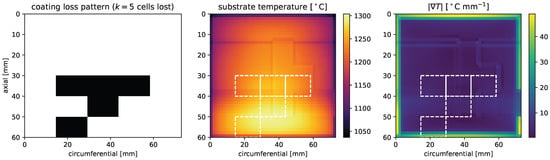
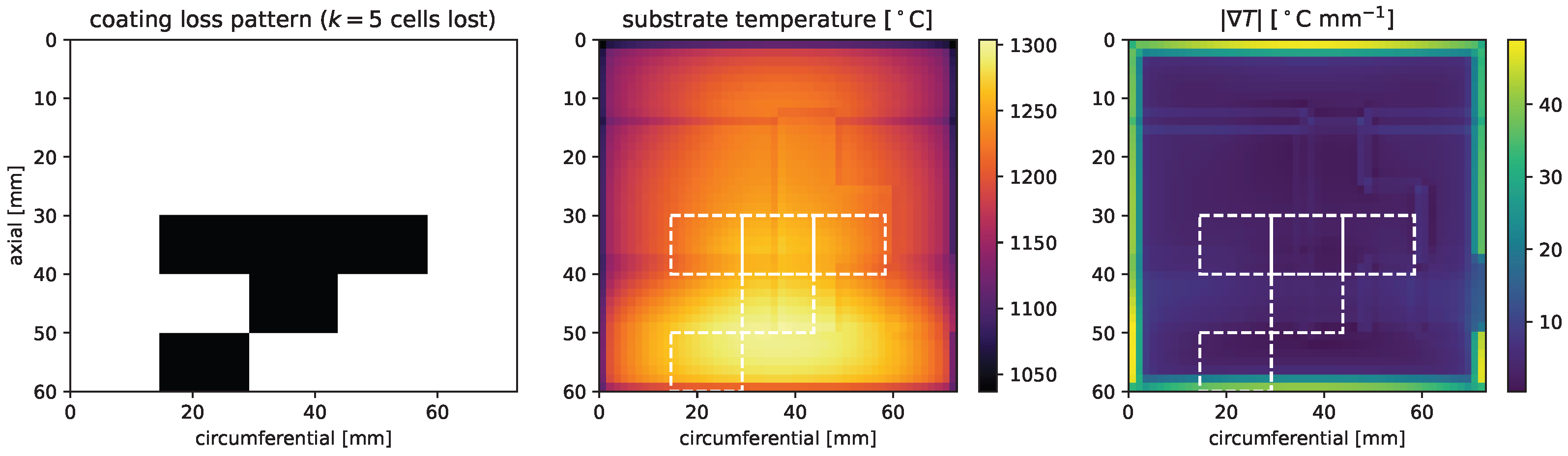
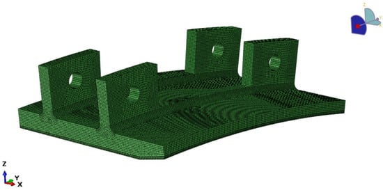
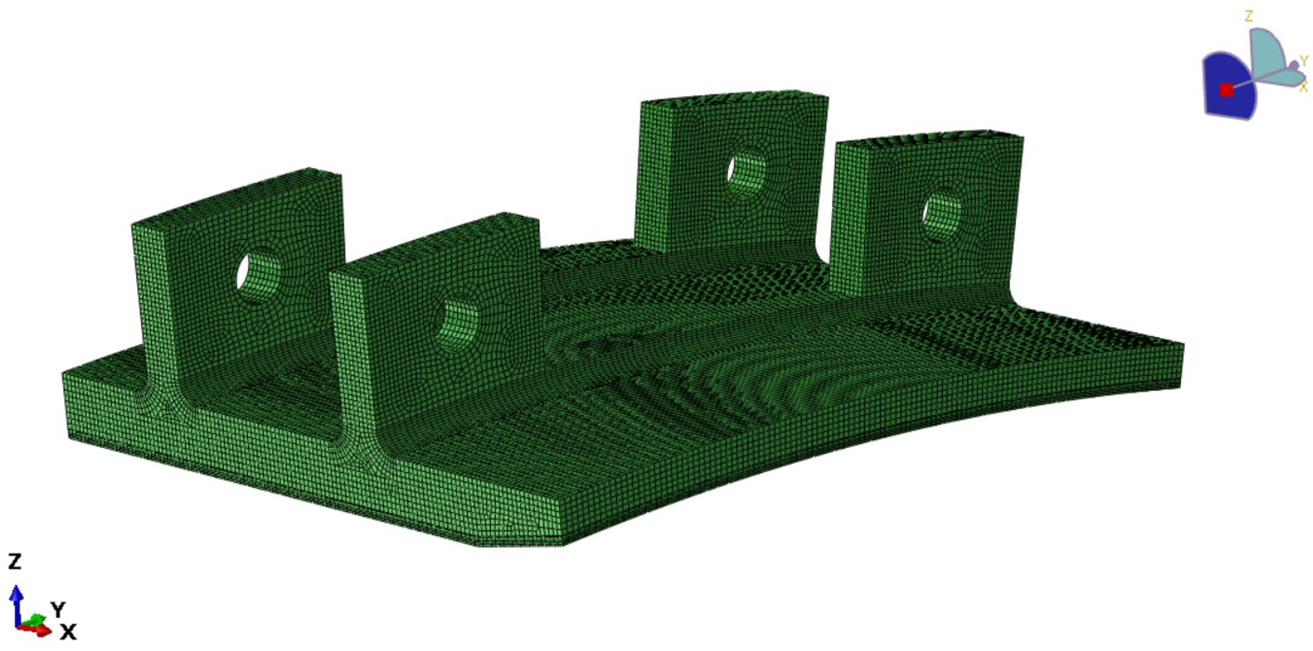
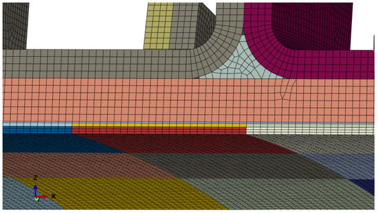
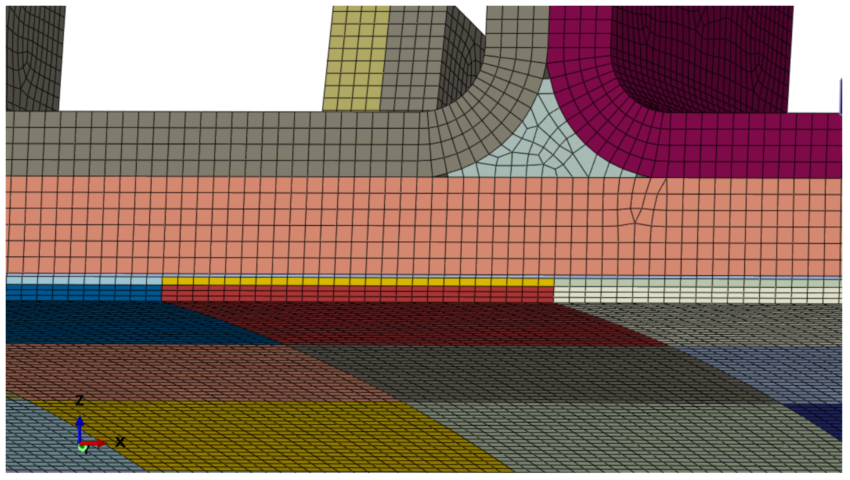
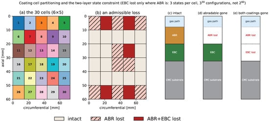
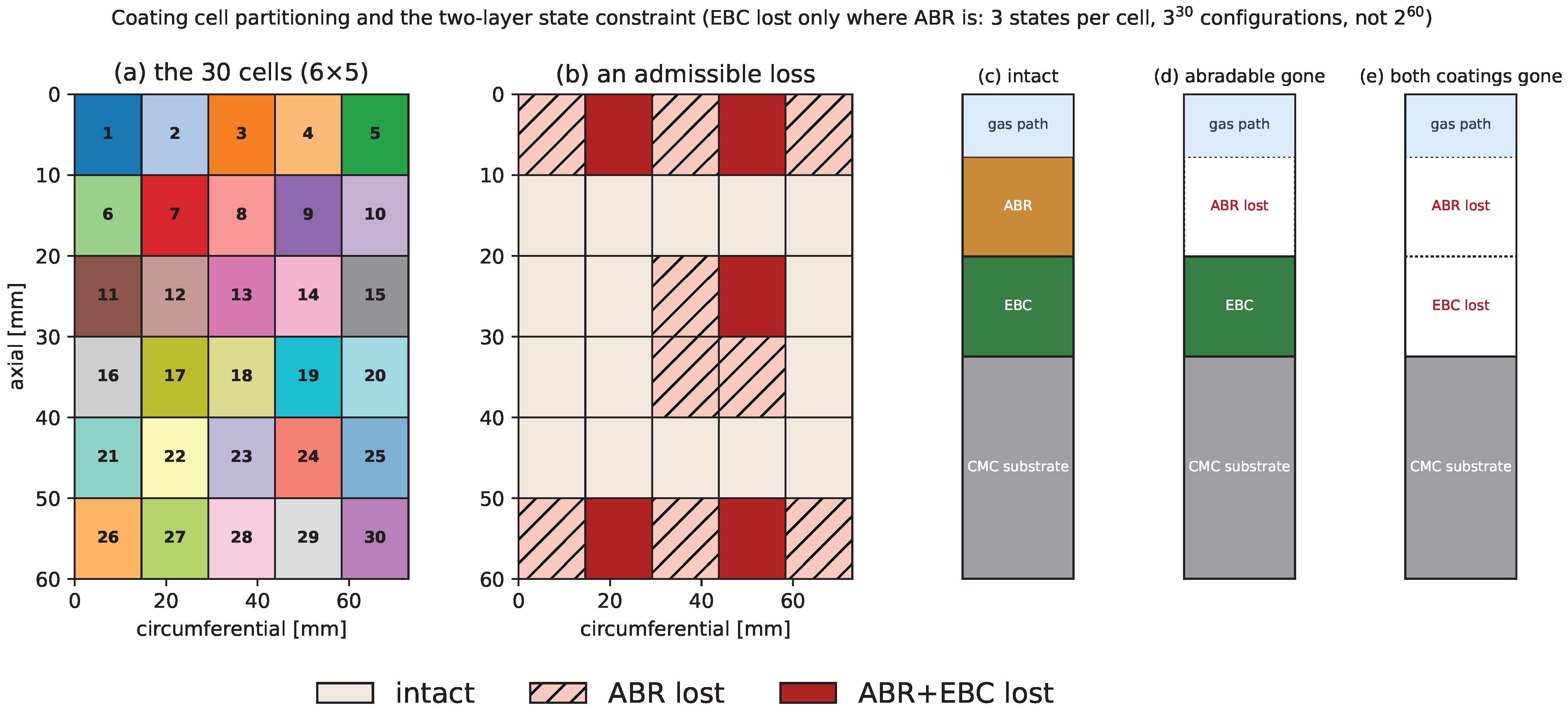
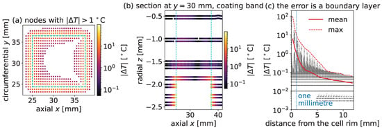
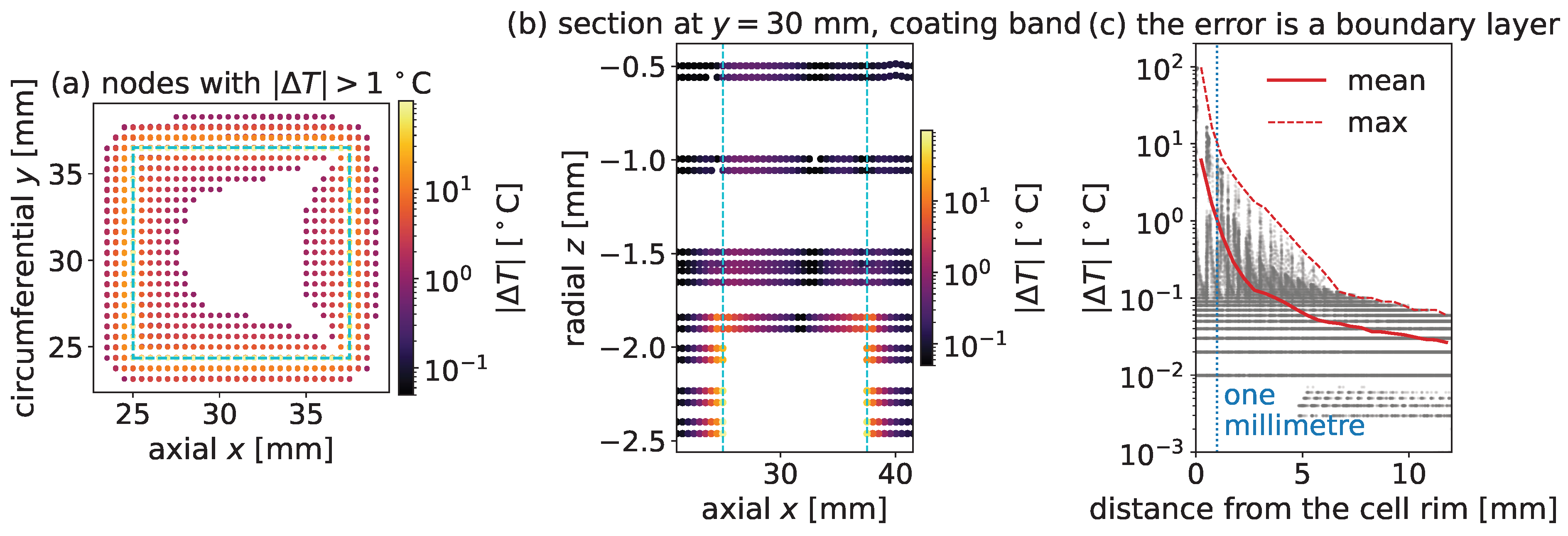
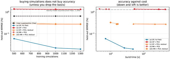
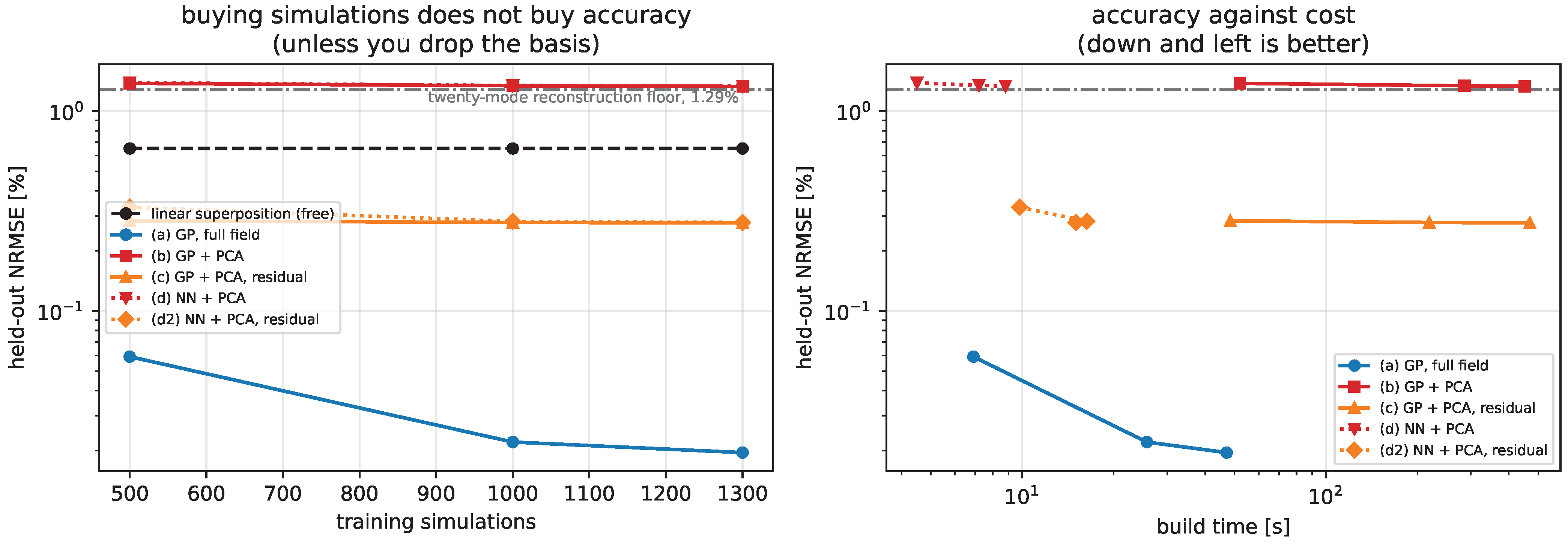
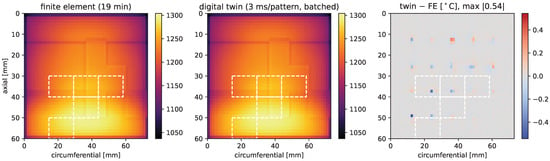
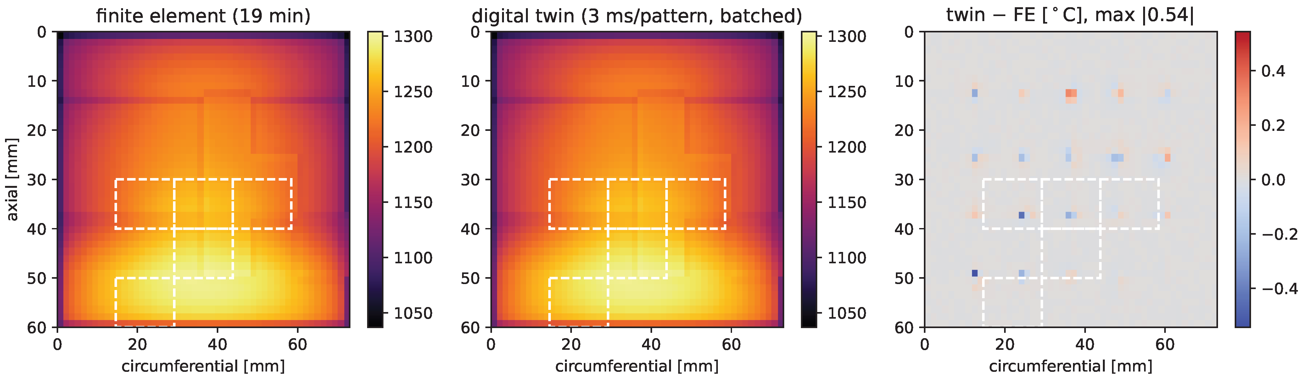
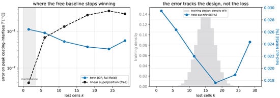
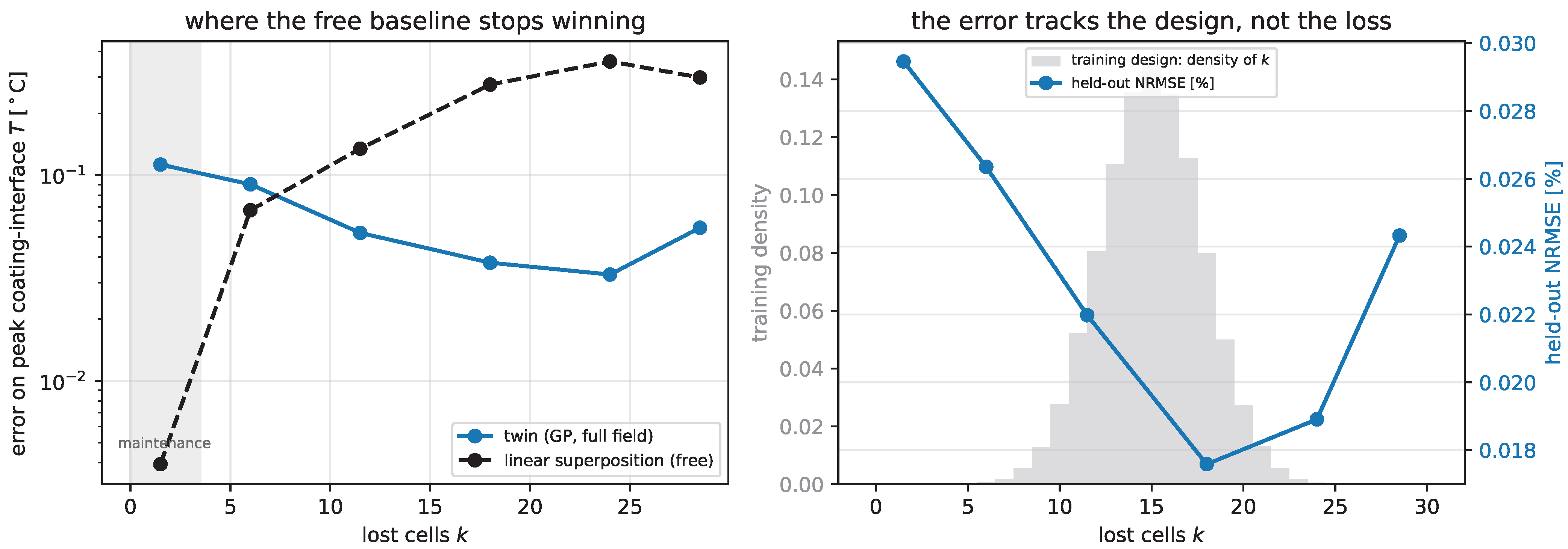
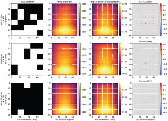
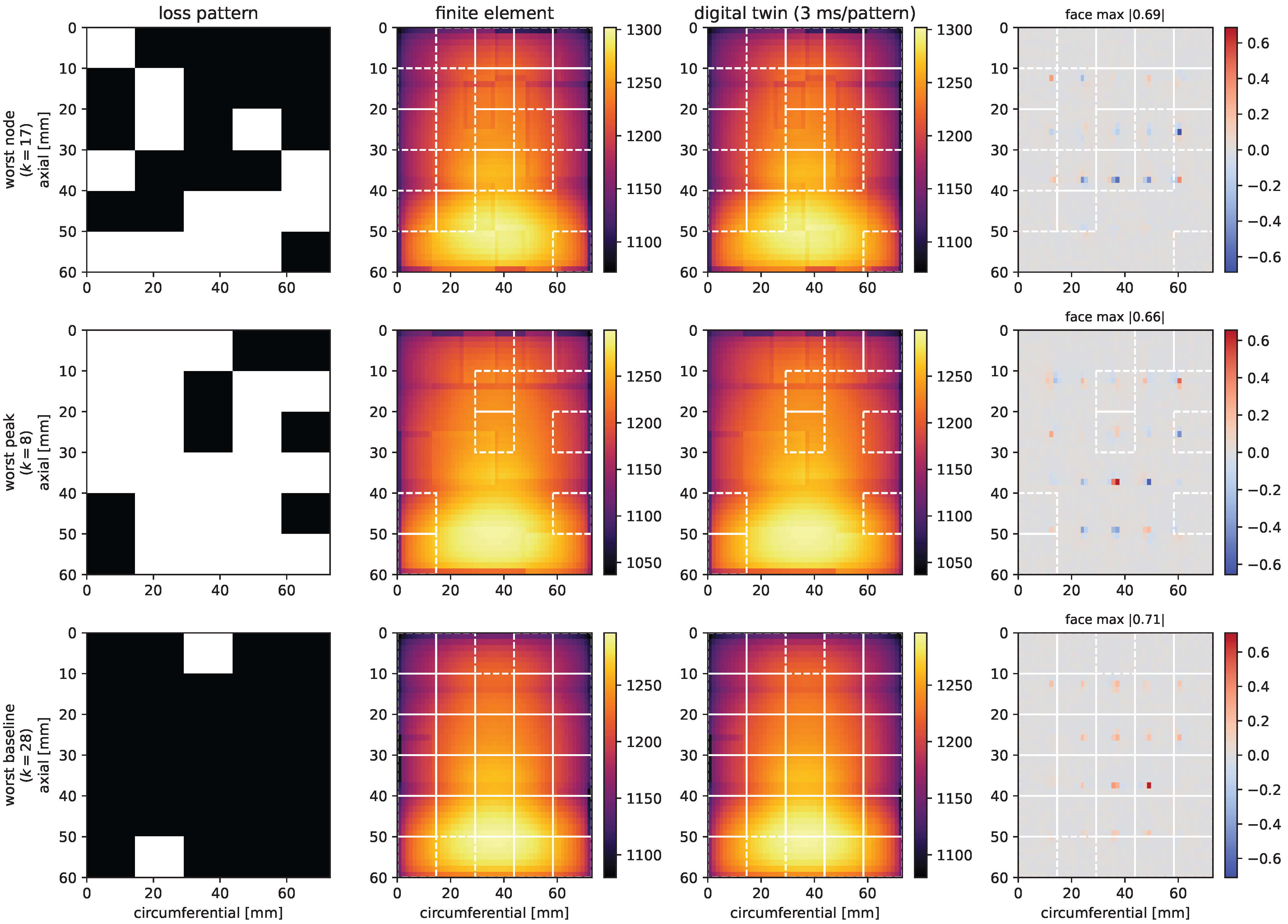
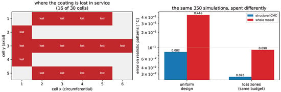
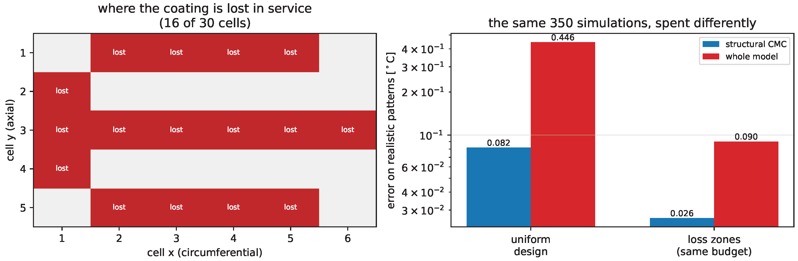
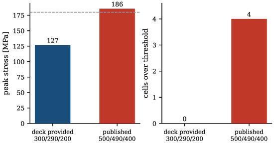
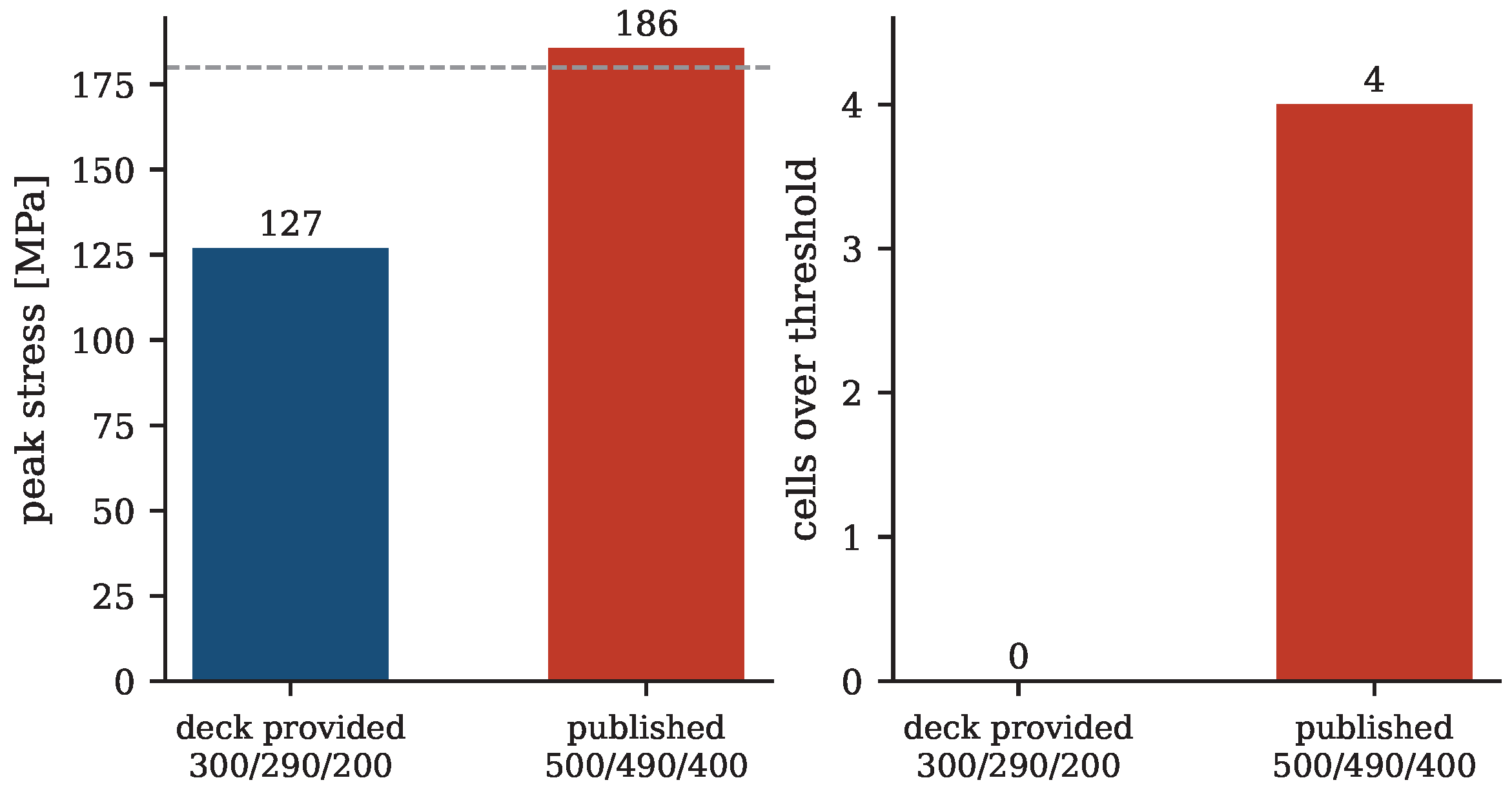
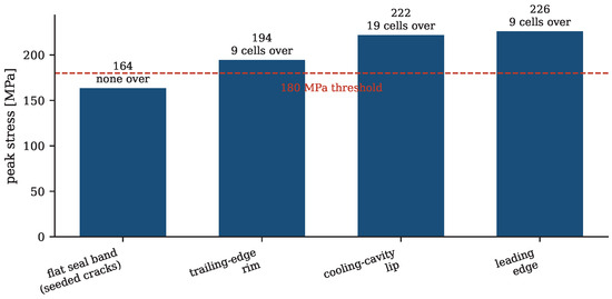
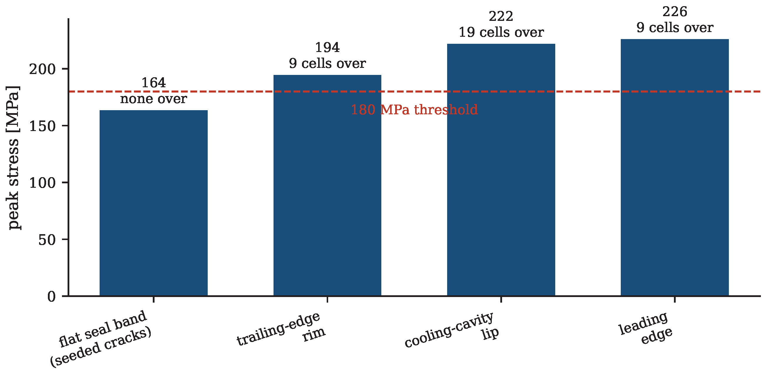
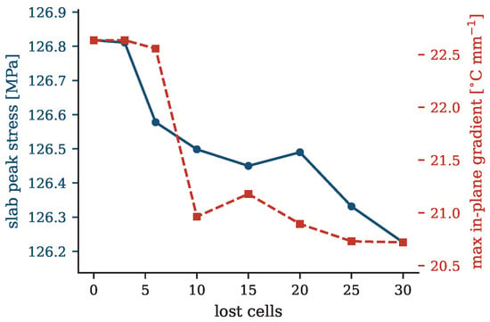
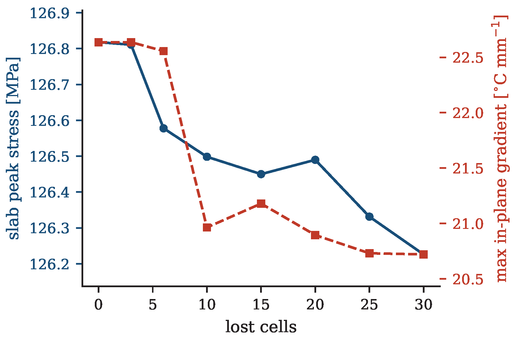
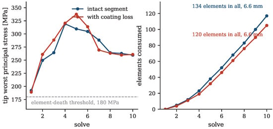
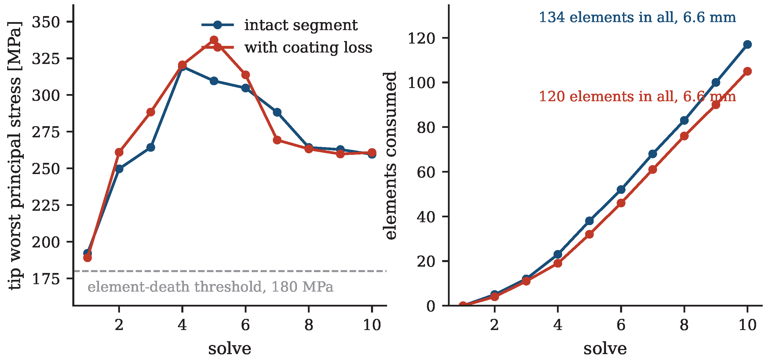

Disclaimer/Publisher’s Note: The statements, opinions and data contained in all publications are solely those of the individual author(s) and contributor(s) and not of MDPI and/or the editor(s). MDPI and/or the editor(s) disclaim responsibility for any injury to people or property resulting from any ideas, methods, instructions or products referred to in the content. |
© 2026 by the authors. Licensee MDPI, Basel, Switzerland. This article is an open access article distributed under the terms and conditions of the Creative Commons Attribution (CC BY) license.