Temporal-Correlated Deep Learning-Based GNSS Signal Classification in the Built Environment: A Comparative Experiment ^†

Abstract

As a key provider of Positioning, Navigation, and Timing (PNT) information, the characteristics of Global Navigation Satellite System (GNSS) signals, including types, Quality Indicators (QIs), and measurements, should be understood. This study employs temporally correlated deep learning models to classify GNSS signals as Line-of-Sight (LOS) or non-LOS using four QIs: the elevation angle, Carrier to Noise Ratio (C/N₀), code measurement’s standard deviation, and difference in azimuth angle. Autocorrelation analysis confirmed that these QIs exhibit significant temporal dependencies. The Bidirectional LSTM (Bi-LSTM) model, with four hidden layers, 64 units, and a sequence length of 18, achieved the best performance: 94.17% classification accuracy and a 2.61% False Positive (FP) rate. Positioning based on classified LOS signals significantly improved accuracy, reducing the mean errors in the horizontal, vertical, and 3D domain by 36.6%, 81.4%, and 59.6%, respectively, and reducing the Standard Deviation (STDEV) by 46.3%, 33.5%, and 45.5%, respectively. Moreover, the non-LOS probability output enables flexible signal selection and mitigates the issue of insufficient signal availability. These results highlight the effectiveness of temporally correlated models in GNSS signal classification and positioning performance.

1. Introduction

As a key provider of PNT information, GNSS offers worldwide coverage, supports standardisation, and facilitates sophisticated antennas, receivers, and auxiliary equipment [1]. Currently, over 120 operational GNSS satellites are available, and the number of satellites visible in open-sky areas typically ranges from 20 to 40 [2].

GNSS data can either be utilised as stand-alone data for PNT applications or integrated with data from other sensors. Regardless of the approach, it is essential to understand the characteristics of GNSS signals, including types, QIs, and measurements. Signals of specific types or those with significant measurement errors must be detected and subsequently corrected or excluded to ensure positioning accuracy and integrity. Moreover, QIs play a pivotal role as input features for classifying signal types and detecting faulty measurements.

GNSS signals can be commonly classified into four categories: LOS, Non-Line-of-Sight (NLOS), multipath, and blocked. Signals are deemed blocked when obstructions completely hinder their reception. LOS signals are received directly by a receiver without any obstructions. Multipath signals are received via multiple paths. Finally, NLOS signals are those diffracted, reflected, or refracted by surrounding obstructions.

GNSS signals at lower elevation angles are more likely to be blocked or interfered with by surrounding obstructions, potentially becoming NLOS or multipath signals, or non-LOS signals. These signals are prone to destructive interference, which reduces signal strength and increases multipath errors [1]. Such interference can also distort the receiver’s correlation function, alter signal polarisation, and cause inconsistencies in GNSS code measurements [3,4,5]. As a result, non-LOS signals are more likely to exhibit characteristics such as low elevation angles, reduced signal strength, altered polarisation, and inconsistent code measurements. These QIs can serve as effective input features for machine learning-based signal classification [4,6,7].

Although several studies on machine learning-based signal classification have been conducted, most treat QIs as a given moment, neglecting their temporal dynamics. Consequently, there has been limited exploration of advanced deep learning architectures, such as Long Short-Term Memory (LSTM) and the Gated Recurrent Unit (GRU), which can capture time-dependent signal characteristics. To address these limitations, this paper novelly invents a temporally correlated deep learning-based approach for GNSS signal classification to estimate non-LOS probabilities, increase classification accuracy, reduce the FP rate, and finally improve positioning accuracy. Section 2 presents a review of machine learning methods for GNSS signal classification. Section 3 describes the GNSS machine learning dataset. Section 4 details the experimental results, followed by the conclusions in Section 5.

2. Review of Machine Learning-Based GNSS Signal Classification Algorithms

Previous studies have labelled received signals into LOS- and non-LOS-using methods such as 3D city models, fisheye imagery, shadow matching, receiver-grade comparisons, and thresholds based on code residuals or C/N₀ [8,9,10]. QIs are frequently used as features for machine learning-based signal classification in preprocessing, including elevation and C/N₀ masking, to exclude faulty measurements. Two metrics are often utilised to evaluate the classification performance, which are the following:

1.

Classification accuracy: The ratio of correctly classified signals to the total number of signals;

2.

FP rate: The ratio of non-LOS signals classified as LOS to the total number of signals. Such misclassification may lead to the inclusion of faulty signals in positioning, potentially degrading accuracy and integrity.

Early work relied on a single QI. Sun et al. [7] utilised C/N₀ in combination with four machine learning models, which are the Gradient Boosting Decision Tree (GBDT), Decision Tree (DT), Distance-Weighted K-Nearest Neighbor (DW-KNN) and Adaptive Network-Based Fuzzy Inference System (ANFIS), resulting in classification accuracies of 74.1%, 67.3%, 59%, and 66.7%, respectively. Hsu [6] individually tested four distinct QIs as inputs to an Supporting Vector Machine (SVM) classifier: C/N₀, the change rate of C/N₀ $\Delta \mathrm{C}/{\mathrm{N}}_0$, code measurement residual ${\epsilon }_p$, and the difference between the delta code measurement and the code measurement rate $\Delta p-\dot{p}\Delta t$. The corresponding classification accuracies were 67.1%, 39.4%, 40.5%, and 65.4%, respectively.

Recent studies have improved GNSS signal classification by incorporating additional QIs. Hsu [6] explored Quality Indicator (QI) combinations such as C/N₀ with $\Delta p-\dot{p}\Delta t$, C/N₀ with ${\epsilon }_p$, and $\Delta p-\dot{p}\Delta t$ with ${\epsilon }_p$ using an SVM. The results showed that including C/N₀ improved the classification performance, while the combination of $\Delta p-\dot{p}\Delta t$ and ${\epsilon }_p$ underperforming compared with C/N₀ alone, highlighting the importance of QI relevance over quantity. Sun et al. [7] used C/N₀, the elevation angle, and ${\epsilon }_p$ as inputs to GBDT, DT, DW-KNN, and ANFIS models, achieving average accuracies between 70.7% and 72.8% across three datasets.

Similarly, Xu et al. [8] used the Signal-to-Noise Ratio (SNR), elevation, ${\epsilon }_p$, and $C_{{\Delta }_p}$ in an SVM model, obtaining 71.8% accuracy with a 24.4% FP rate. Luo et al. [10] expanded this to six QIs ${\epsilon }_p$, the elevation angle, C/N₀, $\Delta \mathrm{C}/{\mathrm{N}}_0$, $C_{{\Delta }_p}$, and standard deviation of code measurements $STDE{V}_p$, achieving up to 83.3% accuracy with 12.0% FP using Particle Swarm Optimisation-Enhanced LightGBM with Weighted Least Squares (PSO-LGBM-WLS).

The analysis of prior work reveals a key limitation in machine learning-based GNSS signal classification with QIs as input. Most studies equate all non-LOS signals with faulty measurements, resulting in their complete exclusion. This reduction in signal availability degrades satellite geometry and impairs positioning accuracy, particularly in the built environment, where non-LOS signals account for a significant proportion. Moreover, binary classification overlooks the varying quality and potential usability of non-LOS signals. To address this, Li et al. [11] proposed a probabilistic approach, namely using machine learning to estimate non-LOS probability. With a flexible threshold, signals can be selectively retained. Using a Random Forest (RF) model with four QIs, the pseudorange standard deviation, C/N₀, elevation, and difference in azimuth angle, the classification accuracy reached 93.43% with a 2.81% FP rate, demonstrating the method’s potential to enhance positioning performance.

Furthermore, most prior studies relied on point-wise QIs, neglecting their temporal correlations. However, time-varying patterns, such as a steadily decreasing elevation angle, can indicate a transition to non-LOS conditions and a decline in signal quality. Capturing these dynamics enables the use of QIs as temporal sequences rather than static inputs. This shift supports the applications of temporally correlated deep learning models, such as LSTM and GRU, offering potential for improved classification performance.

Based on these limitations, the subsequent section will present the methodology for machine learning-based GNSS signal classification, including analysis of the QIs and classification results.

3. Methodology

In the study by Li et al. [11], four QIs, the pseudorange standard deviation, C/N₀, elevation, and difference in azimuth angle, were selected from 10 based on Exploratory Data Analysis (EDA) and feature importance assessments, with a total importance value exceeding 0.95. Prior to temporally correlated deep learning regression, it is essential to evaluate the temporal dependencies of these four QIs with Autocorrelation Function (ACF) results.

Subsequently, four selected temporally correlated deep learning models, namely LSTM, GRU, Convolutional Neural Network LSTM (CNN-LSTM), and Bi-LSTM [12,13,14,15], were utilised for signal classification. LSTM introduces a memory cell and three gates, input, forget, and output, to effectively regulate information flow. This architecture allowed the model to retain or discard temporal information, thereby mitigating the vanishing gradient problem and enabling learning of long-term dependencies.

The GRU is designed to address long-term dependency issues with fewer parameters than LSTM. It employs two gates—update and reset—where the update gate combines the roles of LSTM’s input and forget gates and the reset gate controls the influence of past states. This structure enables faster training and reduced complexity. However, its simplicity may limit its ability to capture complex temporal patterns.

CNN-LSTM is a hybrid model that combines the spatial feature extraction capabilities of the Convolutional Neural Network (CNN) with the temporal modelling strengths of LSTM. CNN layers first extract local patterns from input sequences, which are then passed to LSTM layers to capture temporal dependencies. This architecture is well-suited for data with both spatial and temporal characteristics.

Bi-LSTM is an extension of the standard LSTM designed to process sequential data in both forward and backward directions. This dual-direction processing entails the collaboration of two LSTMs, merging their outputs at every temporal juncture and thereby empowering the network to assimilate time series data in both progressive and regressive sequences. Therefore, Bi-LSTM exhibits a superior capability in recognising intricate patterns and offers an exhaustive understanding of sequential data. However, this enhancement incurs increased computational intricacy and augmented memory requirements as the network effectively doubles in scale by integrating twin LSTM layers.

Instead of merely approaching this task as binary classification, this paper employs regression algorithms to estimate the probability of non-LOS signals. These signals are then classified by comparing their probabilities with a predetermined threshold. The threshold can be adjusted based on the specific requirements of applications. Consequently, this method allows for tailored classification, detection, and exclusion of potential faulty non-LOS signals, aiming to minimise FPs while maintaining sufficient classification accuracy.

Subsequently, based on the required number of signals for positioning, the system is designed to exclude possible faulty non-LOS signals with great probability values. This method mitigates a common issue in binary classification, where excessive non-LOS signals are classified and excluded, which could lead to insufficient signals or suboptimal satellite geometry.

4. Dataset Description

The GNSS data used in this study originated from an open-source dataset by Chemnitz University of Technology, collected in Berlin and Frankfurt, Germany [9]. It includes detailed urban driving routes near key landmarks, such as Frankfurt’s Commerzbank Tower. The data collection employed a mass-market U-blox EVK-M8T GNSS receiver paired with an ANN-MS patch antenna, a reference NovAtel SPAN differential GNSS receiver equipped with a GPS-703-GGG pinwheel antenna, and an odometry sensor. The ground truth was established by merging NovAtel receiver data with ego-motion information from the post-processing phase obtained from a Controller Area Network (CAN) sensor.

The dataset includes the Global Positioning System (GPS) week and seconds of the week, ground truth receiver position, heading, velocity, acceleration, and yaw rate of the vehicle, derived from NovAtel and ego-motion data. Ephemeris data were obtained from the International GNSS Service (IGS). Constellation and satellite identifiers, raw measurements, estimated standard deviations, carrier phase lock times, and C/N₀ were generated using U-blox data. Labelling signals as LOS and non-LOS was accomplished by comparing the signal timespan and availability recorded by both NovAtel and U-blox receivers [9]. Several studies have utilised this dataset to classify and detect non-LOS signals [11,16,17].

The data were collected in four regions, each with a non-LOS signal ratio exceeding $30\%$. To avoid data imbalance and enhance the accuracy and reliability of classification results, part of the LOS signals was randomly removed to equalise the number of the two signal categories. Moreover, this dataset comprises GPS and GLONASS signals, with over 97.92% of the recorded periods featuring more than 10 signals received concurrently.

The dataset was then formulated to support machine learning analysis by aggregating all essential QIs and correlating them with LOS and non-LOS labels. It contains 46,656 LOS and non-LOS signals each. The dataset was segmented into training, validation, and testing datasets randomly distributed at proportions of $52.5\%$, $17.5\%$, and $30\%$, respectively.

5. Results

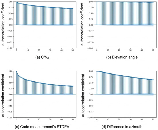
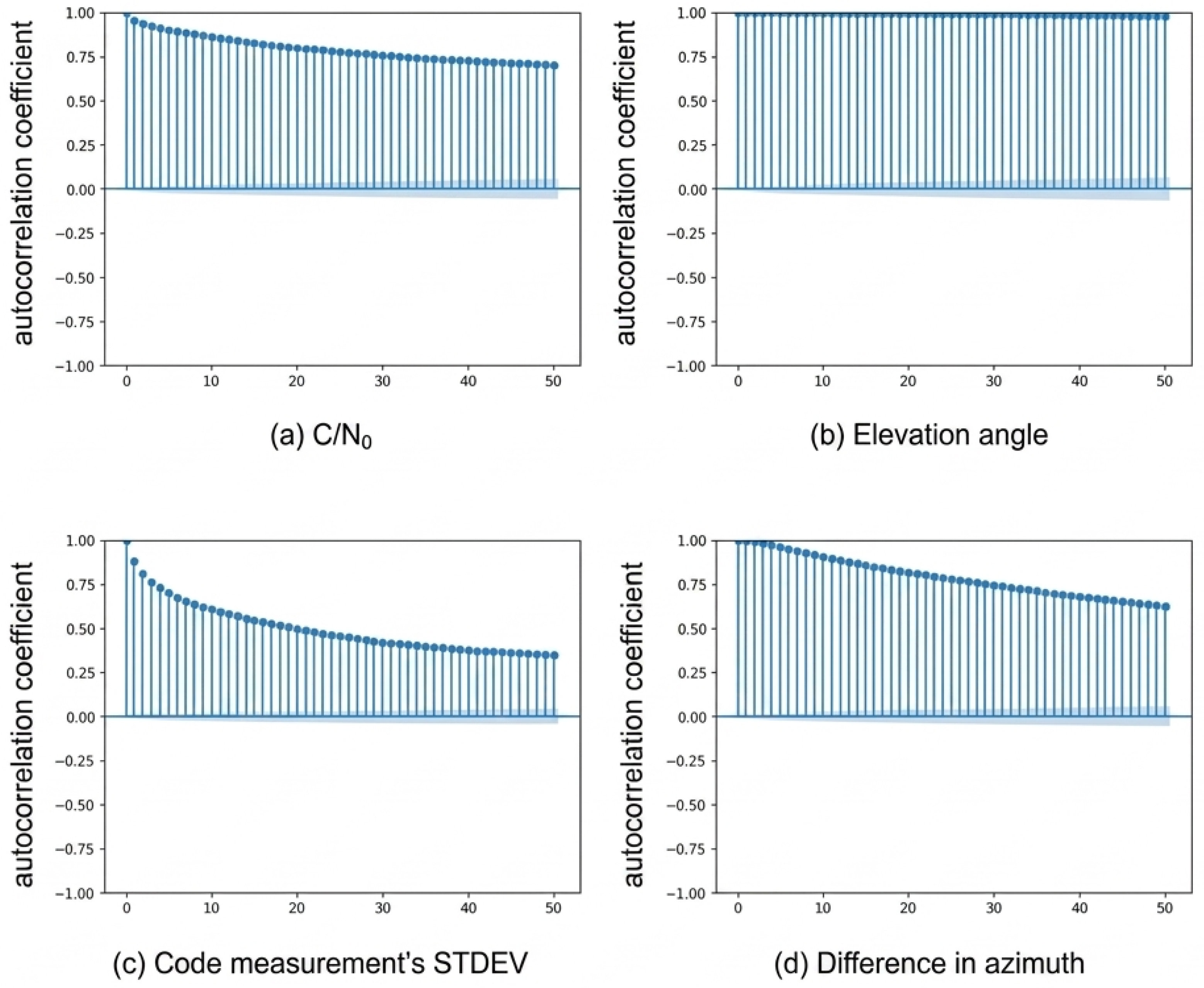
The ACF results in Figure 1 demonstrate that all four QIs exhibited notable temporal dependencies, with each showing significant autocorrelation in varying degrees and patterns. C/N₀ and the elevation angle displayed high initial autocorrelation that declined but remained positive across all lags, indicating a persistent influence of past values over time, an important property for time series prediction. In contrast, the standard deviation of code measurements and the difference in the azimuth angle also exhibited strong initial autocorrelation, but it attenuated more rapidly. Although their influence was less persistent, these features remain valuable for short-term predictions in a deep learning framework.

Figure 1. ACF results for four QIs.

The performance of temporally correlated deep learning models is influenced by their architecture, specifically the temporal sequence length, number of hidden layers, and hidden layer size. In our experiment, the sequence length was initially fixed at 10, while the other two parameters were varied during training and testing. After iterations, all models reached convergence. Table 1 presents a comprehensive performance analysis of four models, where “Layers/Size” represents the number of hidden layers and the size of the hidden layers.

Table 1. Results of signal classification using temporally correlated deep learning models.

Layers/Size	LSTM Acc (%)/FP (%)	GRU Acc (%)/FP (%)	CNN-LSTM Acc (%)/FP (%)	Bi-LSTM Acc (%)/FP (%)
1/16	85.10/8.13	84.15/8.40	84.37/8.42	84.36/8.51
2/16	86.13/7.43	85.70/7.97	84.74/8.39	86.97/7.48
3/16	87.05/7.43	86.21/7.93	85.08/7.73	87.58/7.01
4/16	87.71/7.08	87.10/7.53	84.43/7.56	88.77/6.54
1/32	86.51/7.66	85.84/8.01	85.12/8.23	86.41/7.85
2/32	88.95/6.47	87.53/7.36	86.28/7.98	89.76/5.58
3/32	90.47/5.52	89.48/6.07	86.48/7.51	91.06/4.94
4/32	91.05/5.06	90.48/5.54	86.23/7.94	92.02/4.18
1/64	88.97/6.24	88.19/7.15	85.55/8.38	89.21/6.08
2/64	92.55/3.87	91.33/4.88	87.67/6.94	92.76/3.79
3/64	92.94/3.31	92.81/3.61	87.71/7.22	93.16/3.46
4/64	92.60/3.81	93.00/3.50	90.16/6.10	93.17/3.52

A clear trend observed from the data is improved model performance with increasing complexity, both in the number and size of layers. Specifically, the Bi-LSTM model consistently outperformed the others across all configurations, achieving the highest accuracy and lowest FP rate of 97.17% and 3.52%, respectively, with four hidden layers and 64 hidden units. This suggests that Bi-LSTM, with its bidirectional processing, is particularly effective for this task.

LSTM consistently achieved higher accuracy and lower FP rates than the GRU. GRU models, known for their training efficiency due to fewer parameters and simpler architecture, remain a practical choice when computational resources are limited or faster training is required, despite a modest trade-off in performance. The CNN-LSTM model exhibited inferior performance in comparison with the other models. This indicates that the four QIs chosen and utilised in the other models successfully captured the essential information, hence limiting the potential for the CNN to contribute substantial value in this particular situation.

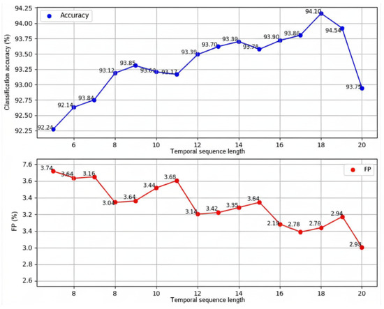
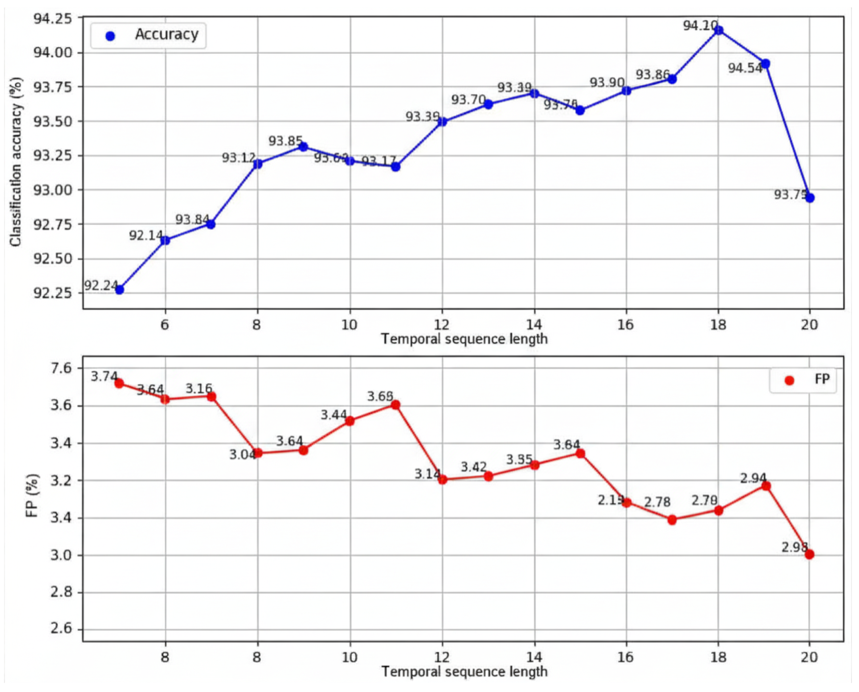
Based on the optimal Bi-LSTM structure, classification performance was further analysed by varying the temporal sequence length. As shown in Figure 2, increasing the sequence length initially improved the accuracy and reduced the false positive rate. However, performance declined when the length exceeded 18. The optimal length was thus 18, achieving a classification accuracy of 94.17% and a false positive rate of 2.61%.

Figure 2. The relationship between the classification performance and the length of the temporal sequence for the optimal Bi-LSTM model.

Compared with the point-wise machine learning models evaluated in Li et al. [11], the temporally correlated deep learning models demonstrated superior classification performance, underscoring the value of incorporating temporal sequences. The Bi-LSTM model, with four hidden layers, 64 units, and a sequence length of 18, excluded 45.20% of the signals, 98.42% of which were non-LOS. In contrast, the RF model excluded 45.56% of the signals, with 97.75% being non-LOS. Among the models, Bi-LSTM excluded the fewest signals while achieving the highest proportion of correctly identified non-LOS instances. Table 2 lists the numbers and ratios of LOS and non-LOS signals whose residual code measurement errors exceeded a specified threshold and were classified as non-LOS. The table also highlights performance differences between the RF and Bi-LSTM models; the RF model more accurately identified non-LOS signals, while Bi-LSTM performed better in correctly classifying LOS signals.

Table 2. The ratio of LOS and non-LOS signals with residual code measurement errors exceeding the specified absolute threshold. These signals were classified as non-LOS by the three models.

Threshold (m)	LOS	Classified	Ratio (%)	Non-LOS	Classified	Ratio (%)
DT
1	44,803	6371	14.22	41,731	35,848	85.90
5	39,857	5718	14.35	39,351	34,000	86.40
10	34,649	5097	14.71	36,762	31,893	86.76
50	11,075	1989	17.96	17,875	16,210	90.69
100	938	425	45.31	6902	6513	94.36
200	60	22	36.67	1073	1064	99.16
RF
1	44,803	937	2.09	41,731	40,962	98.16
5	39,857	838	2.10	39,351	38,661	98.25
10	34,649	753	2.17	36,762	36,143	98.32
50	11,075	268	2.42	17,875	17,650	98.74
100	938	51	5.44	6902	6875	99.61
200	60	2	3.33	1073	1072	99.91
Bi-LSTM
1	44,803	658	1.47	41,731	40,911	98.04
5	39,857	593	1.49	39,351	38,603	98.10
10	34,649	526	1.52	36,762	36,081	98.15
50	11,075	181	1.63	17,875	17,575	98.32
100	938	29	3.09	6902	6846	99.19
200	60	2	3.33	1073	1068	99.53

The positioning results using the original least squares estimation are shown in Table 3. The elevation angle and C/N₀ masks were set to 10 degrees and 10 decibels-Hertz (dB-Hz), respectively. The results show that applying these masks improved all positioning accuracy metrics except the horizontal standard deviation.

Table 3. Positioning results under different signal conditions and masking strategies.

Signal	Masks	Horizontal (m)		Vertical (m)		3D (m)
		Mean	STDEV	Mean	STDEV	Mean	STDEV
All	No	25.75	21.13	71.36	50.51	78.47	51.81
All	Yes	24.98	22.76	60.32	40.41	67.35	41.36
LOS	Yes	15.83	12.21	11.20	26.87	27.18	22.55
≥6	Yes	23.15	23.40	33.02	44.68	46.04	42.85

Using the Bi-LSTM model’s output labels, the classified LOS signals were used for positioning, with results shown in Table 3. The positioning accuracy based on signal classification was significantly improved, further highlighting the value of classification in achieving Failure Detection and Exclusion (FDE) during preprocessing. Compared with using all signals with masking, using only LOS signals improved the horizontal, vertical, and 3D mean positioning errors by 36.6%, 81.4%, and 59.6%, respectively. The Standard Deviation (STDEV) was also reduced by 46.3% (horizontal), 33.5% (vertical), and 45.5% (3D), indicating more stable performance.

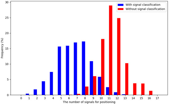
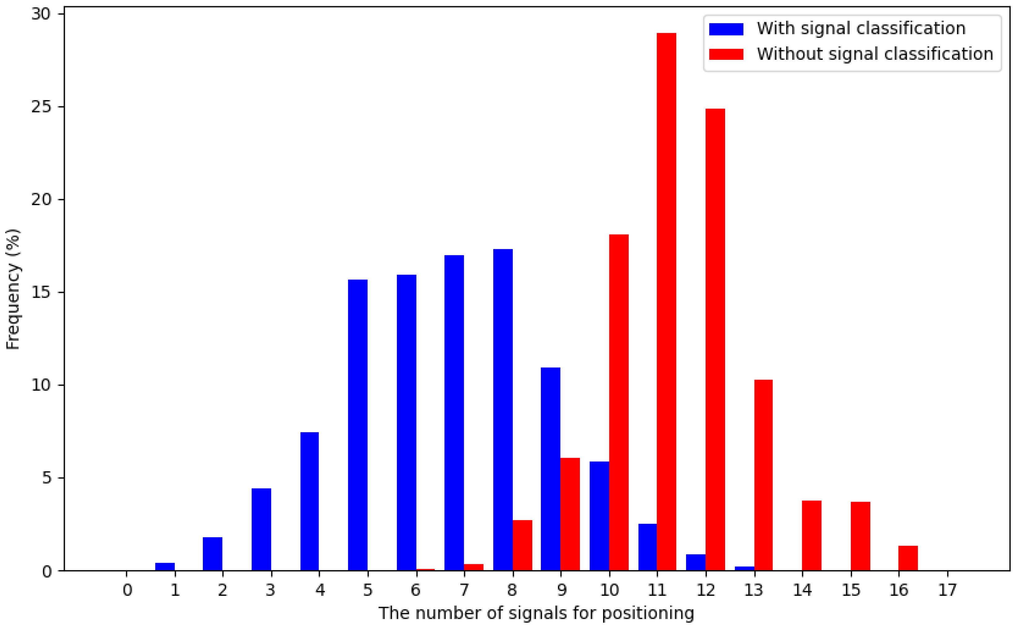
Although the positioning accuracy improved, the number of excluded signals before positioning also increased, potentially resulting in epochs where positioning became impossible due to insufficient signals. Figure 3 illustrates the number of usable signals per epoch with and without signal classification. With two masks applied, all epochs had at least six signals for positioning. However, when both masks and signal classification were used, 29.64% of the epochs contained fewer than six signals, making positioning impossible in nearly 30% of cases even when signals from two constellations were available.

Figure 3. Histogram of the number of signals for positioning with and without signal classification.

To mitigate this issue, the signal subsets were supplemented, with a few signals exhibiting relatively low non-LOS probabilities. The positioning results, based on epochs where positioning was successfully completed, are shown in Table 3. Compared with using all signals with elevation and C/N₀ masks, selecting at least six signals with the lowest non-LOS probabilities yielded substantial improvements in vertical and 3D mean positioning accuracy. However, other metrics showed only marginal improvements or slight degradations, likely due to the omission of satellite geometry, an important consideration for future work.

6. Discussion

Improved classification performance results in more LOS signals being correctly identified. However, this may also increase residual code measurement errors, as some included LOS signals could still contain significant errors. Future research will focus on maintaining classification accuracy while identifying erroneous LOS signals, in conjunction with the satellite geometry considerations discussed earlier.

7. Conclusions

The autocorrelation analysis confirmed that all four selected QIs exhibited significant temporal dependencies, validating the use of temporally correlated models for GNSS signal classification. Among the evaluated architectures, the Bi-LSTM model with four hidden layers, 64 units, and a temporal sequence length of 18 achieved the best performance, yielding a classification accuracy of 94.17% and an FP rate of 2.61%, outperforming the RF model overall. While the RF model was more effective at identifying non-LOS signals, Bi-LSTM demonstrated superior accuracy in classifying LOS signals.

Positioning based on classified LOS signals significantly improved the accuracy, reducing mean errors in the horizontal, vertical, and 3D domain by 36.6%, 81.4%, and 59.6%, respectively, and reducing the STDEV by 46.3%, 33.5%, and 45.5%, respectively, compared with conventional masking-based approaches. Furthermore, the non-LOS probability enabled more flexible signal selection strategies, mitigating the issue of insufficient signals for positioning after classification. These findings highlight the effectiveness of GNSS signal classification with temporally correlated deep learning models in enhancing both signal quality assessment and positioning performance.

References

- Groves, P.D. Principles of GNSS, inertial, and multisensor integrated navigation systems, 2nd edition [Book review]. IEEE Aerosp. Electron. Syst. Mag. 2015, 30, 26–27. [Google Scholar] [CrossRef] [Scilit]
- Haozhang, Z.; Pan, L. Current performance of open position service with almost fully deployed multi-GNSS constellations: GPS, GLONASS, Galileo, BDS-2, and BDS-3. Adv. Space Res. 2022, 69, 1994–2019. [Google Scholar] [CrossRef] [Scilit]
- Groves, P.D.; Jiang, Z.; Rudi, M.; Strode, P. A portfolio approach to NLOS and multipath mitigation in dense urban areas. In Proceedings of the 26th International Technical Meeting of the Satellite Division of The Institute of Navigation (ION GNSS+ 2013), Nashville, TN, USA, 16–20 September 2013. [Google Scholar]
- Bassma, G.; Tayeb, S. GNSS positioning enhancement based on NLOS multipath biases estimation using gaussian mixture noise. Int. J. Mob. Comput. Multimed. Commun. 2018, 9, 21–39. [Google Scholar] [CrossRef] [Scilit]
- Zhu, N.; Marais, J.; Bétaille, D.; Berbineau, M. GNSS position integrity in urban environments: A review of literature. IEEE Trans. Intell. Transp. Syst. 2018, 19, 2762–2778. [Google Scholar] [CrossRef] [Scilit]
- Hsu, L.T. GNSS multipath detection using a machine learning approach. In Proceedings of the 2017 IEEE 20th International Conference on Intelligent Transportation Systems (ITSC), Yokohama, Japan, 16–19 October 2017; pp. 1–6. [Google Scholar]
- Sun, R.; Wang, G.; Zhang, W.; Hsu, L.T.; Ochieng, W.Y. A gradient boosting decision tree based GPS signal reception classification algorithm. Appl. Soft Comput. 2020, 86, 105942. [Google Scholar] [CrossRef] [Scilit]
- Xu, H.; Angrisano, A.; Gaglione, S.; Hsu, L.T. Machine learning based LOS/NLOS classifier and robust estimator for GNSS shadow matching. Satell. Navig. 2020, 1, 15. [Google Scholar] [CrossRef] [Scilit]
- Reisdorf, P.; Pfeifer, T.; Breßler, J.; Bauer, S.; Weissig, P.; Lange, S.; Wanielik, G.; Protzel, P. The problem of comparable GNSS results–an approach for a uniform dataset with low-cost and reference data. In Proceedings of the International Conference on Advances in Vehicular Systems, Technologies and Applications (VEHICULAR), Barcelona, Spain, 13–17 November 2016. [Google Scholar]
- Luo, H.; Liu, J.; He, D. GNSS Signal Labeling, Classification and Positioning in Urban Scenes Based on PSO-LGBM-WLS Algorithm. IEEE Trans. Instrum. Meas. 2023, 72, 2528213. [Google Scholar] [CrossRef] [Scilit]
- Li, L.; Elhajj, M.; Feng, Y.; Ochieng, W.Y. Machine learning based GNSS signal classification and weighting scheme design in the built environment: A comparative experiment. Satell. Navig. 2023, 4, 12. [Google Scholar] [CrossRef] [Scilit]
- Sherstinsky, A. Fundamentals of recurrent neural network (RNN) and long short-term memory (LSTM) network. Phys. D Nonlinear Phenom. 2020, 404, 132306. [Google Scholar] [CrossRef] [Scilit]
- Dey, R.; Salem, F.M. Gate-variants of gated recurrent unit (GRU) neural networks. In Proceedings of the 2017 IEEE 60th International Midwest Symposium on Circuits and Systems (MWSCAS), Boston, MA, USA, 6–9 August 2017; pp. 1597–1600. [Google Scholar]
- Kim, T.Y.; Cho, S.B. Predicting residential energy consumption using CNN-LSTM neural networks. Energy 2019, 182, 72–81. [Google Scholar] [CrossRef] [Scilit]
- Hamayel, M.J.; Owda, A.Y. A novel cryptocurrency price prediction model using GRU, LSTM and Bi-LSTM machine learning algorithms. AI 2021, 2, 477–496. [Google Scholar] [CrossRef] [Scilit]
- Li, F.; Dai, Z.; Li, T.; Zhu, X. GNSS NLOS signals identification based on deep neural networks. In Proceedings of the 4th International Conference on Information Science, Electrical, and Automation Engineering (ISEAE 2022), Guangzhou, China, 25–27 March 2022; Volume 12257, pp. 160–169. [Google Scholar]
- Reisdorf, P.; Wanielik, G. Approach for Self-consistent NLOS Detection in GNSS multi constellation Based Localization. In Proceedings of the 31st International Technical Meeting of the Satellite Division of The Institute of Navigation (ION GNSS+ 2018), Miami, FL, USA, 24–28 September 2018; pp. 3663–3670. [Google Scholar]
Disclaimer/Publisher’s Note: The statements, opinions and data contained in all publications are solely those of the individual author(s) and contributor(s) and not of MDPI and/or the editor(s). MDPI and/or the editor(s) disclaim responsibility for any injury to people or property resulting from any ideas, methods, instructions or products referred to in the content. |
© 2026 by the authors. Licensee MDPI, Basel, Switzerland. This article is an open access article distributed under the terms and conditions of the Creative Commons Attribution (CC BY) license.