Quantum Theory and Unusual Dielectric Functions of Graphene

Abstract

We address the spatially nonlocal dielectric functions of graphene at any frequency derived starting from the first principles of thermal quantum field theory using the formalism of the polarization tensor. After a brief review of this formalism, the longitudinal and transverse dielectric functions are considered at any relationship between the frequency and the wave vector. The analytic properties of their real and imaginary parts are investigated at low and high frequencies. Emphasis is given to the double pole at zero frequency, which arises in the transverse dielectric function. The role of this unusual property in solving the problem of disagreement between experiment and theory in the Casimir effect is discussed. We believe that a more complete dielectric response of ordinary metals should also be spatially nonlocal and its transverse part may possess the double pole in the region of evanescent waves.

1. Introduction

It is common knowledge that quantum physics originated in 1900 from the work of Max Planck, who derived the distribution law for the monochromatic radiation, and introduced the concept of the quantum of energy and the new fundamental constant h, now known as the Planck constant [1]. In 1905, Albert Einstein arrived at a concept of the quanta of light, which were later called photons, and explained on this basis the photoelectric effect [2]. However, the first quantum theory—quantum mechanics—was created one hundred years ago by Werner Heisenberg (1925) [3] and Erwin Schödinger (1926) [4]. The relativistic quantum mechanics formulated by Paul Dirac in 1928 [5] introduced the concept of antiparticles and opened a path to the formulation of quantum field theory and its applications to all fundamental interactions of nature during the twentieth century.

For a long time, it was believed that quantum theory is only needed to describe very small submicroscopic objects on atomic and even subatomic scales. Later it was understood, however, that there are numerous macroscopic quantum phenomena characterized by scales greatly exceeding the atomic ones. These are the superconductivity, superfluidity, quantum Hall and Josephson effects, Bose–Einstein condensation, the Casimir effect, and others. Currently, the macroscopic quantum phenomena are not of only an academic interest, but are widely used in many technological and industrial applications, as well as in metrology.

Considerable recent attention has been focussed on various novel materials described by quantum theory, and the two-dimensional sheet of carbon atoms called graphene occupies a prominent place among them. Graphene is remarkable for many reasons, including its unique mechanical, electrical, and optical properties [6,7,8]. At energies below approximately 3 eV, graphene is quite well described by the Dirac model. This means that the field of either massless or very light electronic quasiparticles in graphene satisfies the (2 + 1)-dimensional Dirac equation rather than the Schrödinger equation, which describes the standard quasiparticles considered in condensed matter physics. In doing so, the Fermi velocity in graphene $v_F\approx c/300$ that plays the same role as the speed of light c in the usual Dirac equation.

The response of graphene to the electromagnetic field is spatially nonlocal. It is commonly described by the tensors of electric conductivity or dielectric permittivity. For a graphene sheet in the absence of constant magnetic field, these tensors are characterized by two functions, each depending on frequency $\omega$, the two-dimensional wave vector $\mathit{q}$, and on temperature $T$ (for gapped and doped, graphene, these tensors also depend on the mass gap parameter and chemical potential). These functions are the longitudinal ${\sigma }^{\mathrm{L}}$ and transverse ${\sigma }^{\mathrm{T}}$ conductivities and the corresponding dielectric functions ${\epsilon }^{\mathrm{L}}$ and ${\epsilon }^{\mathrm{T}}$. In the case of two spatial dimensions, the dielectric functions are expressed in terms of conductivities as [9,10]

$${\epsilon }^{\mathrm{L},\mathrm{T}}(\omega ,\mathit{q})=1+{\displaystyle \frac{2\pi \mathit{iq}}{\omega }}{\sigma }^{\mathrm{L},\mathrm{T}}(\omega ,\mathit{q}),$$

(1)

where $q=\left|\mathit{q}\right|=\sqrt{q_1^2+q_2^2}$. That is, in the Gaussian units used here and throughout the paper, the conductivities of graphene have the dimension of cm/s (for the three-dimensional materials, the dimension of conductivity is 1/s).

The response functions of graphene were investigated in both the spatially local ($\mathit{q}=0,{\epsilon }^{\mathrm{L}}={\epsilon }^{\mathrm{T}}=\epsilon$) and nonlocal cases using a number of more or less phenomenological approaches, such as the hydrodynamic model [11,12,13], Boltzmann transport theory and the Drude model [14,15,16,17,18,19,20,21,22], current–current correlation functions and the random phase approximation [23,24,25,26,27,28,29,30,31,32], density-functional theory [33,34], Kubo response theory [35,36,37,38,39,40,41,42,43,44,45,46], modeling graphene optics in terms of Lorentz-type oscillators [47] and by using the Fresnel reflection coefficients [48], and others (see also the reviews [49,50,51]). The obtained results have different levels of accuracy and different areas of application. In the framework of the Dirac model, however, the response functions of graphene can be found exactly starting from the first principles of thermal quantum field theory using the formalism of the polarization tensor in (2 + 1)-dimensions.

In this paper, we discuss the properties of the longitudinal and transverse dielectric functions of graphene expressed in the framework of quantum field theory via the components of the polarization tensor. The dependence of these functions on frequency is investigated over the entire region of positive frequencies (the dependence of the dielectric functions of graphene on temperature is investigated in Ref. [52]). It is shown that these functions possess some standard properties characteristic of common materials. Thus, they satisfy the Kramers–Kronig relations, go to unity with an indefinitely increasing frequency, and have the positive imaginary parts as it must be in accordance with the second law of thermodynamics [53]. At the same time, we demonstrate that the transverse dielectric function of graphene possesses an unusual property by having the double pole at zero frequency (it is generally believed that at zero frequency the response functions of metallic and dielectric materials have a single pole and are regular, respectively). We propose that in the region of evanescent waves, the transverse dielectric function of ordinary metals may have a double pole as well.

We start in Section 2 with a brief review of the most necessary results regarding the polarization tensor of graphene. Then, in Section 3, we consider the properties of dielectric functions of graphene expressed via a polarization tensor at low frequencies. Section 4 is devoted to the case of high frequencies. Section 5 and Section 6 contain the discussion and conclusions. For the sake of clarity in presentation, all mathematical equations are written for the case of a pristine graphene possessing the zero mass gap parameter and chemical potential. However, all the results presented remain valid for the gapped and doped graphene sheets.

2. Polarization Tensor of Graphene

In the one-loop approximation, the interaction of electronic quasiparticles in graphene with the electromagnetic field is described by the quasiparticle loop diagram having two photon legs. It is represented by the polarization tensor ${\mathrm{\Pi }}_{\mu \nu }$, where the Greek letter indices take the values $0,1,$ and 2. At zero temperature, the polarization tensor has long been calculated using (2+1)-dimensional quantum field theory [54,55]. Specifically, for graphene, whose properties are temperature-dependent, the polarization tensor was studied in detail at both zero and nonzero temperature [35,56,57,58,59,60]. In the latter case, the formalism of thermal quantum field theory in the Matsubara formulation was used.

The expressions for the polarization tensor of graphene valid over the entire plane of complex frequency, including the real frequency axis, were obtained in Refs. [61,62] (the previously obtained expressions [60] are valid only at the pure imaginary Matsubara frequencies). The expressions of Refs. [61,62] were used for investigation of the electric conductivity [63,64,65,66] and reflectivity [67,68,69] of graphene, as well as of the Casimir and Casimir–Polder forces in out-of-thermal-equilibrium graphene systems [70,71,72,73,74,75].

All components of the polarization tensor can be expressed via the two independent quantities [60], for example, via ${\mathrm{\Pi }}_{00}$ and

$$\mathrm{\Pi }(\omega ,\mathit{q})=q^2{\mathrm{\Pi }}_{\mu }^{\mu }(\omega ,\mathit{q})+\left({\displaystyle \frac{{\omega }^2}{c^2}}-q^2\right){\mathrm{\Pi }}_{00}(\omega ,\mathit{q}).$$

(2)

There are different but mathematically equivalent representations for the quantities ${\mathrm{\Pi }}_{00}$ and $\mathrm{\Pi }$. In this paper, the representations from Ref. [70] are used.

Note that the entire range of positive frequencies from zero to infinity can be divided into the regions of evanescent, $0<\omega <\mathit{cq}$, and propagating, $\omega ⩾\mathit{cq}$, waves. In the region of evanescent waves, it is convenient to separate the subregion of strongly evanescent waves, $0<\omega <v_{F}q$. The explicit expressions for ${\mathrm{\Pi }}_{00}$ and $\mathrm{\Pi }$ have different forms in the regions $0<\omega <v_{F}q$ and $\omega >v_{F}q$. We start with the region $0<\omega <v_{F}q$, i.e., with strongly evanescent waves. In this region, for ${\mathrm{\Pi }}_{00}$ one has [70]

$$\begin{array}{ccc}& & \mathrm{Re}{\mathrm{\Pi }}_{00}(\omega ,\mathit{q})={\displaystyle \frac{\pi \alpha \mathit{\hslash }c{q}^2}{\sqrt{v_F^2{q}^2-{\omega }^2}}}+{\displaystyle \frac{8\alpha \mathit{\hslash }c}{v_F^2}}\left\{\phantom{\left[\underset{0}{\overset{v_{F}q-\omega }{\int }}{\displaystyle \frac{\mathit{dx}}{e^{\beta x}+1}}\right]}{\displaystyle \frac{\ln 2}{\beta }}\right.\hfill \\ & & \left.+{\displaystyle \frac{1}{2\sqrt{v_F^2{q}^2-{\omega }^2}}}\left[\underset{0}{\overset{v_{F}q-\omega }{\int }}{\displaystyle \frac{\mathit{dx}}{e^{\beta x}+1}}{F}_1\left(x\right)-\underset{0}{\overset{v_{F}q+\omega }{\int }}{\displaystyle \frac{\mathit{dx}}{e^{\beta x}+1}}{F}_2\left(x\right)\right]\right\}\hfill \end{array}$$

(3)

and

$$\mathrm{Im}{\mathrm{\Pi }}_{00}(\omega ,\mathit{q})={\displaystyle \frac{4\alpha \mathit{\hslash }c}{v_F^2\sqrt{v_F^2{q}^2-{\omega }^2}}}\left[\underset{v_{F}q-\omega }{\overset{\infty }{\int }}{\displaystyle \frac{\mathit{dx}}{e^{\beta x}+1}}{F}_3\left(x\right)-\underset{v_{F}q+\omega }{\overset{\infty }{\int }}{\displaystyle \frac{\mathit{dx}}{e^{\beta x}+1}}{F}_4\left(x\right)\right],$$

(4)

where $\alpha =e^2/(\mathit{\hslash }c)$ is the fine structure constant with $e$ the elementary charge, ℏ is the reduced Planck constant, $\beta =\mathit{\hslash }/\left(2k_{B}T\right)$, $k_B$ is the Boltzmann constant, and

$$F_{1,2}\left(x\right)=\sqrt{v_F^2{q}^2-{(x\pm \omega )}^2},F_{3,4}\left(x\right)=\sqrt{{(x\pm \omega )}^2-v_F^2{q}^2}.$$

In a similar way, for $\mathrm{\Pi }$ one obtains [70]

$$\begin{array}{ccc}& & \mathrm{Re}\mathrm{\Pi }(\omega ,\mathit{q})={\displaystyle \frac{\pi \alpha \mathit{\hslash }{q}^2}{c}}\sqrt{v_F^2{q}^2-{\omega }^2}+{\displaystyle \frac{8\alpha \mathit{\hslash }}{v_F^{2}c}}\left\{\phantom{\left[\underset{0}{\overset{v_{F}q-\omega }{\int }}{\displaystyle \frac{\mathit{dx}}{e^{\beta x}+1}}\right]}{\displaystyle \frac{{\omega }^2\ln 2}{\beta }}\right.\hfill \\ & & \left.+{\displaystyle \frac{\sqrt{v_F^2{q}^2-{\omega }^2}}{2}}\left[\underset{0}{\overset{v_{F}q-\omega }{\int }}{\displaystyle \frac{\mathit{dx}}{e^{\beta x}+1}}{\displaystyle \frac{{(x+\omega )}^2}{F_1\left(x\right)}}-\underset{0}{\overset{v_{F}q+\omega }{\int }}{\displaystyle \frac{\mathit{dx}}{e^{\beta x}+1}}{\displaystyle \frac{{(x-\omega )}^2}{F_2\left(x\right)}}\right]\right\}\hfill \end{array}$$

(5)

and

$$\mathrm{Im}\mathrm{\Pi }(\omega ,\mathit{q})={\displaystyle \frac{4\alpha \mathit{\hslash }}{v_F^{2}c}}\sqrt{v_F^2{q}^2-{\omega }^2}\left[\underset{v_{F}q+\omega }{\overset{\infty }{\int }}{\displaystyle \frac{\mathit{dx}}{e^{\beta x}+1}}{\displaystyle \frac{{(x-\omega )}^2}{F_4\left(x\right)}}-\underset{v_{F}q-\omega }{\overset{\infty }{\int }}{\displaystyle \frac{\mathit{dx}}{e^{\beta x}+1}}{\displaystyle \frac{{(x+\omega )}^2}{F_3\left(x\right)}}\right].$$

(6)

In the remaining region of evanescent waves $v_{F}q<\omega <\mathit{cq}$ and in the region of propagating waves $\omega ⩾\mathit{cq}$, the quantities ${\mathrm{\Pi }}_{00}$ and $\mathrm{\Pi }$ are given by the unified expressions [70]. Thus, for ${\mathrm{\Pi }}_{00}$ one has

$$\begin{array}{ccc}& & \mathrm{Re}{\mathrm{\Pi }}_{00}(\omega ,\mathit{q})={\displaystyle \frac{4\alpha \mathit{\hslash }c}{v_F^2}}\left\{\phantom{\left[\underset{0}{\overset{v_{F}q-\omega }{\int }}{\displaystyle \frac{\mathit{dx}}{e^{\beta x}+1}}\right]}{\displaystyle \frac{2\ln 2}{\beta }}\right.-{\displaystyle \frac{1}{\sqrt{{\omega }^2-v_F^2{q}^2}}}\hfill \\ & & \left.\times \left[\underset{0}{\overset{\infty }{\int }}{\displaystyle \frac{\mathit{dx}}{e^{\beta x}+1}}{F}_3\left(x\right)-\underset{\omega +v_{F}q}{\overset{\infty }{\int }}{\displaystyle \frac{\mathit{dx}}{e^{\beta x}+1}}{F}_4\left(x\right)+\underset{0}{\overset{v_{F}q-\omega }{\int }}{\displaystyle \frac{\mathit{dx}}{e^{\beta x}+1}}{F}_4\left(x\right)\right]\right\}\hfill \end{array}$$

(7)

and

$$\mathrm{Im}{\mathrm{\Pi }}_{00}(\omega ,\mathit{q})={\displaystyle \frac{\alpha \mathit{\hslash }c}{\sqrt{{\omega }^2-v_F^2{q}^2}}}\left[\pi q^2-{\displaystyle \frac{4}{v_F^2}}\underset{-v_{F}q}{\overset{v_{F}q}{\int }}\mathit{dx}{\displaystyle \frac{\sqrt{v_F^2{q}^2-x^2}}{e^{\beta (\omega +x)}+1}}\right].$$

(8)

For $\mathrm{\Pi }$ the following expressions are valid:

$$\begin{array}{ccc}& & \mathrm{Re}\mathrm{\Pi }(\omega ,\mathit{q})={\displaystyle \frac{4\alpha \mathit{\hslash }}{v_F^{2}c}}\left\{\phantom{\left[\underset{0}{\overset{v_{F}q-\omega }{\int }}{\displaystyle \frac{\mathit{dx}}{e^{\beta x}+1}}\right]}{\displaystyle \frac{2{\omega }^2\ln 2}{\beta }}\right.-\sqrt{{\omega }^2-v_F^2{q}^2}\hfill \\ & & \times \left[\underset{0}{\overset{\infty }{\int }}{\displaystyle \frac{\mathit{dx}}{e^{\beta x}+1}}{\displaystyle \frac{{(x+\omega )}^2}{F_3\left(x\right)}}-\underset{\omega +v_{F}q}{\overset{\infty }{\int }}{\displaystyle \frac{\mathit{dx}}{e^{\beta x}+1}}{\displaystyle \frac{{(x-\omega )}^2}{F_4\left(x\right)}}\right.\left.\left.+\underset{0}{\overset{\omega -v_{F}q}{\int }}{\displaystyle \frac{\mathit{dx}}{e^{\beta x}+1}}{\displaystyle \frac{{(x-\omega )}^2}{F_4\left(x\right)}}\right]\right\}\hfill \end{array}$$

(9)

and

$$\mathrm{Im}\mathrm{\Pi }(\omega ,\mathit{q})={\displaystyle \frac{\alpha \mathit{\hslash }}{v_F^{2}c}}\sqrt{{\omega }^2-v_F^2{q}^2}\left[-\pi v_F^2{q}^2+4\underset{-v_{F}q}{\overset{v_{F}q}{\int }}{\displaystyle \frac{\mathit{dx}}{e^{\beta (\omega +x)}+1}}{\displaystyle \frac{x^2}{\sqrt{v_F^2{q}^2-x^2}}}\right].$$

(10)

Note that a summary of the auxiliary functions introduced above and some other notations used in the paper is contained in the Appendix A in Table A1.

The polarization tensor is gauge-invariant and, as a consequence, satisfies the transversality condition [54,55,56,57,58,59,60,61,62]

$$q^{\mu }{\mathrm{\Pi }}_{\mu \nu }(\omega ,\mathit{q})=0,q^{\mu }=(\omega /c,q^1,q^2).$$

(11)

Now, we use an expression for the current,

$$J^{\mu }(\omega ,\mathit{q})={\displaystyle \frac{c}{4\pi \mathit{\hslash }}}{\mathrm{\Pi }}^{\mu \nu }(\omega ,\mathit{q})A_{\nu }(\omega ,\mathit{q}),$$

(12)

arising due an application of the electromagnetic field, with $A_{\nu }$ the vector potential, and the microscopic relativistically covariant Ohm’s law [76]

$$J^{\mu }(\omega ,\mathit{q})={\sigma }^{\mu \nu }(\omega ,\mathit{q})E_{\nu }(\omega ,\mathit{q}),$$

(13)

where ${\sigma }^{\mu \nu }$ is the tensor of electric conductivity and $E_{\nu }$ is the 3-vector of the electric field (see also Ref. [77] for a definition of the relativistically covariant vectors of electric and magnetic fields). Through employing Equations (12) and (13) and $E_{\nu }=(i\omega /c)A_{\nu }$, one expresses the tensor of electric conductivity via the polarization tensor [23,78,79,80,81,82]

$${\sigma }^{\mu \nu }(\omega ,\mathit{q})={\displaystyle \frac{c^2}{4\pi \mathit{\hslash }}}{\displaystyle \frac{{\mathrm{\Pi }}^{\mu \nu }(\omega ,\mathit{q})}{i\omega }}.$$

(14)

With the help of Equation (14), the longitudinal and transverse conductivities of graphene are presented as follows [63,64,65,66]:

$${\sigma }^{\mathrm{L}}(\omega ,\mathit{q})=-{\displaystyle \frac{i\omega }{4\pi \mathit{\hslash }{q}^2}}{\mathrm{\Pi }}_{00}(\omega ,\mathit{q}),{\sigma }^{\mathrm{T}}(\omega ,\mathit{q})={\displaystyle \frac{{\mathrm{ic}}^2}{4\pi \mathit{\hslash }{q}^2\omega }}\mathrm{\Pi }(\omega ,\mathit{q}).$$

(15)

Finally, using Equation (1), for the longitudinal and transverse dielectric functions of graphene, one obtains [63,83]

$${\epsilon }^{\mathrm{L}}(\omega ,\mathit{q})=1+{\displaystyle \frac{1}{2\mathit{\hslash }q}}{\mathrm{\Pi }}_{00}(\omega ,\mathit{q}),{\epsilon }^{\mathrm{T}}(\omega ,\mathit{q})=1-{\displaystyle \frac{c^2}{2\mathit{\hslash }q{\omega }^2}}\mathrm{\Pi }(\omega ,\mathit{q}).$$

(16)

Note that recently the basics of quantum field theoretical approach to describing the electric conductivity and dielectric response of graphene were cast under doubt. It was noticed [84] that some of the results obtained using quantum field theory are in disagreement with those following from the Kubo model. Based on the Kubo formula, the polarization tensor ${\mathrm{\Pi }}^{\mu \nu }$ in Equations (12) and (14) was replaced with the so-called “regularized” quantity ${\tilde{\mathrm{\Pi }}}^{\mu \nu }$ defined as follows: [84]

$${\tilde{\mathrm{\Pi }}}^{\mu \nu }(\omega ,\mathit{q})={\mathrm{\Pi }}^{\mu \nu }(\omega ,\mathit{q})-\underset{\omega \to 0}{\lim }{\mathrm{\Pi }}^{\mu \nu }(\omega ,\mathit{q}).$$

(17)

It was shown, however, that the polarization tensor ${\mathrm{\Pi }}^{\mu \nu }$ is defined uniquely and cannot be modified with no violation of first principles of quantum theory [85]. In Ref. [84], derivation of Equation (15) with ${\tilde{\mathrm{\Pi }}}_{\mu \nu }(\omega ,\mathit{q})$ in place of ${\mathrm{\Pi }}_{\mu \nu }(\omega ,\mathit{q})$ from the Kubo formula used the nonrelativistic concept of causality rather than the relativistic one, as would be correct for the Dirac model. Specifically, Ref. [84] applied the one-sided Fourier transforms from 0 to ∞ instead of the two-sided one from $-\infty$ to ∞, which must be used in the relativistic theory, and obtained the subtracted term in Equation (17), making an integration by parts in the integral from 0 to ∞. This resulted in a violation of the gauge invariance and in other physically unacceptable consequences [86].

Thus, there is no any contradiction between the results obtained using the quantum field theory and the Kubo model if the latter is applied appropriately. When using the two-sided Fourier transforms, as one has to do in application to the relativistic systems, such as graphene, the Kubo formula results in the correct Equation (14) with the polarization tensor ${\mathrm{\Pi }}^{\mu \nu }$ [86].

3. Dielectric Functions of Graphene at Low Frequencies

Here, we consider the properties of both the longitudinal and transverse dielectric functions of graphene in the region of strongly evanescent waves $0<\omega <v_{F}q$. Substituting Equations (3) and (4) in the first equality of Equation (16), the real and imaginary parts of the longitudinal dielectric function read

$$\begin{array}{ccc}& & \mathrm{Re}{\epsilon }^{\mathrm{L}}(\omega ,\mathit{q})=1+{\displaystyle \frac{\pi \alpha cq}{2\sqrt{v_F^2{q}^2-{\omega }^2}}}+{\displaystyle \frac{4\alpha c}{v_F^{2}q}}\left\{\phantom{\left[\underset{0}{\overset{v_{F}q-\omega }{\int }}{\displaystyle \frac{\mathit{dx}}{e^{\beta x}+1}}\right]}{\displaystyle \frac{\ln 2}{\beta }}\right.\hfill \\ & & \left.+{\displaystyle \frac{1}{2\sqrt{v_F^2{q}^2-{\omega }^2}}}\left[\underset{0}{\overset{v_{F}q-\omega }{\int }}{\displaystyle \frac{\mathit{dx}}{e^{\beta x}+1}}{F}_1\left(x\right)-\underset{0}{\overset{v_{F}q+\omega }{\int }}{\displaystyle \frac{\mathit{dx}}{e^{\beta x}+1}}{F}_2\left(x\right)\right]\right\}\hfill \end{array}$$

(18)

and

$$\mathrm{Im}{\epsilon }^{\mathrm{L}}(\omega ,\mathit{q})={\displaystyle \frac{2\alpha c}{v_F^{2}q\sqrt{v_F^2{q}^2-{\omega }^2}}}\left[\underset{v_{F}q-\omega }{\overset{\infty }{\int }}{\displaystyle \frac{\mathit{dx}}{e^{\beta x}+1}}{F}_3\left(x\right)-\underset{v_{F}q+\omega }{\overset{\infty }{\int }}{\displaystyle \frac{\mathit{dx}}{e^{\beta x}+1}}{F}_4\left(x\right)\right].$$

(19)

As is seen in Equations (18) and (19), in the limiting case $\omega \to 0$ one has

$$\begin{array}{ccc}& & \underset{\omega \to 0}{\lim }\mathrm{Re}{\epsilon }^{\mathrm{L}}(\omega ,\mathit{q})=1+{\displaystyle \frac{\pi \alpha c}{2v_F}}+{\displaystyle \frac{8\alpha c\ln 2}{v_F^{2}q}}{\displaystyle \frac{k_{B}T}{\mathit{\hslash }}},\hfill \\ & & \underset{\omega \to 0}{\lim }\mathrm{Im}{\epsilon }^{\mathrm{L}}(\omega ,\mathit{q})=0,\hfill \end{array}$$

(20)

i.e., the longitudinal dielectric function of graphene is regular at zero frequency. From Equation (19), one finds that $\mathrm{Im}{\epsilon }^{\mathrm{L}}(\omega ,\mathit{q})>0$ because the integrand in the first integral is larger than in the second and integrated over the wider interval.

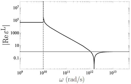
As an example, in Figure 1, $\mathrm{Re}{\epsilon }^{\mathrm{L}}$ (18) is shown at $T=300$ K, with $q=100{\mathrm{cm}}^{-1}$$\approx 1.24\times {10}^{-2}\mathrm{eV}$ as the function of frequency in the region to the left of the vertical dashed line $\omega =v_{F}q\approx {10}^{10}$ rad/s $\approx 6.58\times {10}^{-6}$ eV. When $\omega$ approaches $v_{F}q$, $\mathrm{Re}{\epsilon }^{\mathrm{L}}$ goes to infinity.

Figure 1. The magnitude of real part (18) of the longitudinal dielectric function of graphene versus frequency for $T=300$ K and $q=100{\mathrm{cm}}^{-1}$. The threshold at $\omega =v_{F}q$ is shown by the dashed vertical line.

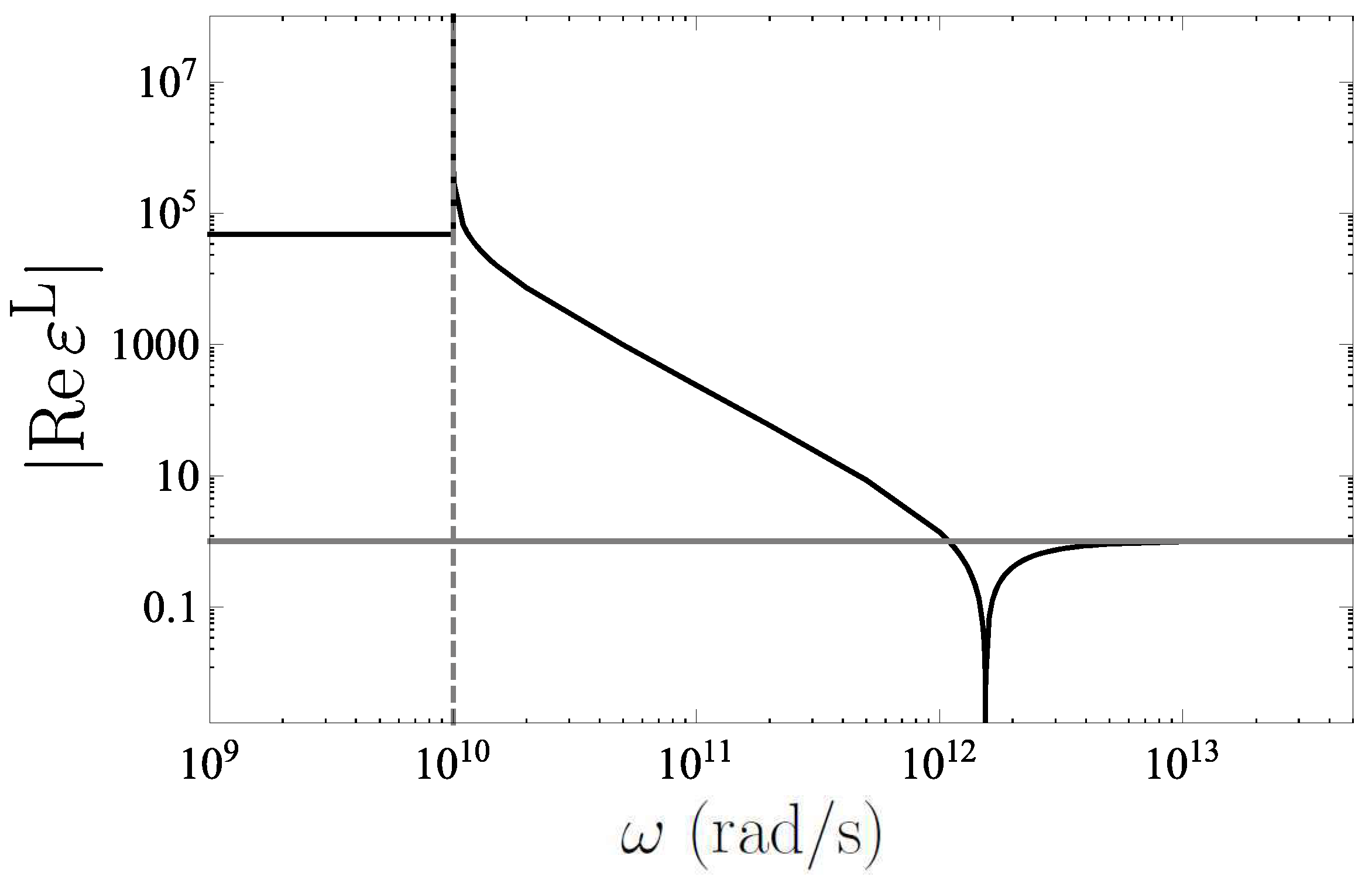
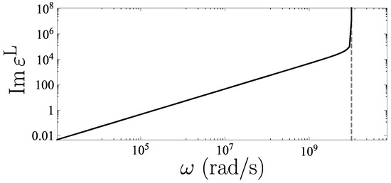
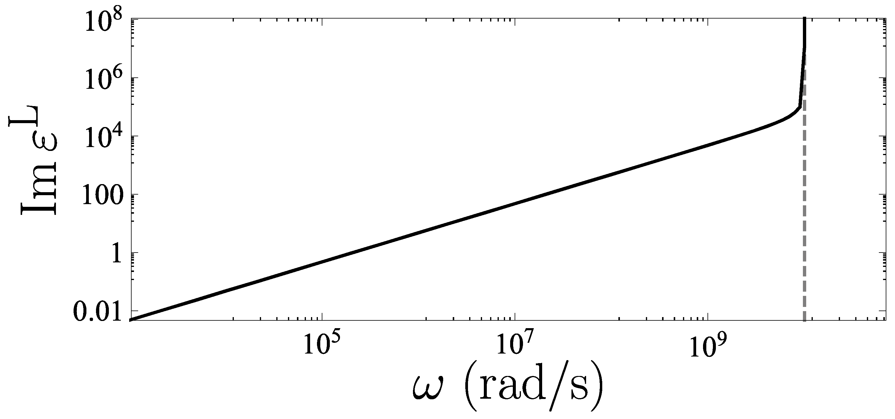
Figure 2 shows the imaginary part $\mathrm{Im}{\epsilon }^{\mathrm{L}}$ (19) of the longitudinal response function of graphene at $T=300$ K and $q=100{\mathrm{cm}}^{-1}$ as the function of frequency in the region to the left of the vertical dashed line $\omega =v_{F}q$. As is seen in Figure 2, $\mathrm{Im}{\epsilon }^{\mathrm{L}}$ goes to infinity when $\omega$ approaches $v_{F}q$ from the left, as does $\mathrm{Re}{\epsilon }^{\mathrm{L}}$.

Figure 2. The imaginary part (19) of the longitudinal dielectric function of graphene versus frequency for $T=300$ K and $q=100{\mathrm{cm}}^{-1}$. The threshold at $\omega =v_{F}q$ is shown by the dashed vertical line.

The real and imaginary parts of the transverse dielectric function of graphene at low frequencies ($\omega <v_{F}q$) are obtained by substituting Equations (5) and (6) into the second equality of Equation (16). The result is

$$\begin{array}{ccc}& & \mathrm{Re}{\epsilon }^{\mathrm{T}}(\omega ,\mathit{q})=1-{\displaystyle \frac{\pi \alpha \mathit{cq}}{2{\omega }^2}}\sqrt{v_F^2{q}^2-{\omega }^2}-{\displaystyle \frac{4\alpha c}{v_F^{2}q}}{\displaystyle \frac{\ln 2}{\beta }}\hfill \\ & & -{\displaystyle \frac{2\alpha c\sqrt{v_F^2{q}^2-{\omega }^2}}{v_F^{2}q{\omega }^2}}\left[\underset{0}{\overset{v_{F}q-\omega }{\int }}{\displaystyle \frac{\mathit{dx}}{e^{\beta x}+1}}{\displaystyle \frac{{(x+\omega )}^2}{F_1\left(x\right)}}-\underset{0}{\overset{v_{F}q+\omega }{\int }}{\displaystyle \frac{\mathit{dx}}{e^{\beta x}+1}}{\displaystyle \frac{{(x-\omega )}^2}{F_2\left(x\right)}}\right]\hfill \end{array}$$

(21)

and

$$\mathrm{Im}{\epsilon }^{\mathrm{T}}(\omega ,\mathit{q})={\displaystyle \frac{2\alpha c}{v_F^{2}q{\omega }^2}}\sqrt{v_F^2{q}^2-{\omega }^2}\left[\underset{v_{F}q-\omega }{\overset{\infty }{\int }}{\displaystyle \frac{\mathit{dx}}{e^{\beta x}+1}}{\displaystyle \frac{{(x+\omega )}^2}{F_3\left(x\right)}}-\underset{v_{F}q+\omega }{\overset{\infty }{\int }}{\displaystyle \frac{\mathit{dx}}{e^{\beta x}+1}}{\displaystyle \frac{{(x-\omega )}^2}{F_4\left(x\right)}}\right].$$

(22)

Now, let us consider the behavior of $\mathrm{Re}{\epsilon }^{\mathrm{T}}$ and $\mathrm{Im}{\epsilon }^{\mathrm{T}}$ in the limiting case $\omega \to 0$. From (21), it is seen that the second term on the right-hand side (r.h.s.) behaves as $-A/{\omega }^2$, where $A=\pi \alpha {\mathit{cv}}_F{q}^2/2$, i.e., $\mathrm{Re}{\epsilon }^{\mathrm{T}}$ has the double pole at $\omega =0$ which is very unusual. Recall that the commonly used Drude dielectric function of metals has the single pole at zero frequency, whereas for dielectrics the dielectric functions are regular at all frequencies. The formal presence of a double pole is typical for the plasma model. In the case of conventional metals, it is applicable only at high frequencies belonging to the far ultraviolet and Roentgen regions [53]. It is worth to note that the case of a double pole appearing in Re${\epsilon }^{\mathrm{T}}$ for graphene is not similar to the plasma oscillations in superconductors, which are described by the dielectric permittivities possessing the double pole at zero frequency [87,88,89,90,91,92,93,94,95]. The point is that the electric current in semiconductors associated with the double pole in the dielectric function is real and depends only on frequency in the local London limit. By contrast, in graphene the double pole is present only at $q\ne 0$ and the associated electric current is pure imaginary.

The behavior of the last term in Equation (21) in the limiting case $\omega \to 0$ is not so evident. To determine it, let us introduce the parameter $\kappa \equiv \omega /\left(v_{F}q\right)$ and perform the changes of variables $t=x/\left(v_{F}q\right)+\kappa$ and $t=x/\left(v_{F}q\right)-\kappa$, respectively, in the first and second integrals in the squared brackets in Equation (21). Then, one obtains

$$\underset{0}{\overset{v_{F}q-\omega }{\int }}{\displaystyle \frac{\mathit{dx}}{e^{\beta x}+1}}{\displaystyle \frac{{(x+\omega )}^2}{F_1\left(x\right)}}-\underset{0}{\overset{v_{F}q+\omega }{\int }}{\displaystyle \frac{\mathit{dx}}{e^{\beta x}+1}}{\displaystyle \frac{{(x-\omega )}^2}{F_2\left(x\right)}}=v_F^2{q}^2(I_1+I_2),$$

(23)

where

$$\begin{array}{ccc}& & I_1=\underset{\kappa }{\overset{1}{\int }}{\displaystyle \frac{t^2\mathit{dt}}{\sqrt{1-t^2}}}\left({\displaystyle \frac{1}{e^{\gamma t}{e}^{-\gamma \kappa }+1}}-{\displaystyle \frac{1}{e^{\gamma t}{e}^{\gamma \kappa }+1}}\right),\hfill \\ & & I_2=\underset{-\kappa }{\overset{\kappa }{\int }}{\displaystyle \frac{\mathit{dt}}{e^{\gamma t}{e}^{\gamma \kappa }+1}}{\displaystyle \frac{t^2}{\sqrt{1-t^2}}},\gamma \equiv v_{F}q\beta .\hfill \end{array}$$

(24)

Under the condition $\omega \ll v_{F}q$, i.e., $\kappa \ll 1$, at fixed $q,T\ne 0$, we expand the integrand in $I_1$ in powers of the small parameter $\beta \kappa$ and obtain

$$I_1=\gamma \kappa B_1+O\left({\gamma }^3{\kappa }^3\right),B_1\equiv 2\underset{0}{\overset{1}{\int }}{\displaystyle \frac{t^2\mathit{dt}}{\sqrt{1-t^2}}}{\displaystyle \frac{e^{\gamma t}}{{(e^{\gamma t}+1)}^2}}.$$

(25)

By making a similar expansion in $I_2$, one finds that in the lowest order $I_2={\kappa }^3/3$ and, thus, it does not contribute to the behavior of $\mathrm{Re}{\epsilon }^{\mathrm{T}}$ at low frequencies.

As a result, substituting Equations (23) and (25) into Equation (21), for the low-frequency behavior of the real part of transverse dielectric function of graphene, one finds

$$\mathrm{Re}{\epsilon }^{\mathrm{T}}(\omega ,\mathit{q})=1-8\ln 2{\displaystyle \frac{\alpha c}{v_F^{2}q}}{\displaystyle \frac{k_{B}T}{\mathit{\hslash }}}-{\displaystyle \frac{\alpha \mathit{\hslash }{\mathit{cv}}_F{q}^2}{k_{B}T}}{\displaystyle \frac{B_1}{\omega }}-{\displaystyle \frac{\pi \alpha {\mathit{cv}}_F{q}^2}{2{\omega }^2}}.$$

(26)

Note that the “regularized” polarization tensor (17) was introduced in Ref. [84] aiming removing the last term in Equation (26), which was considered in Ref. [84] as “nonphysical”. The presence of this term, however, is in agreement with all physical principles and was confirmed experimentally by measuring the Casimir force in graphene systems [96,97]. Using the current–current correlation functions [27] and the polarization tensor [60], it was predicted that in the systems with a graphene layer at nonzero temperature the Casimir force reaches high-temperature asymptotics equal to one-half of that valid for ideal metals already at short separations. According to Ref. [27], for graphene the high-temperature regime is reached under the condition ${\mathit{ak}}_{B}T\gtrsim \mathit{\hslash }{v}_F\approx 0.0033\mathit{\hslash }c$, where $a$ denotes the separation distance between two graphene sheets. Using the formalism of the polarization tensor, Ref. [60] indicated the application condition of the high-temperature regime for the system of a pristine graphene sheet parallel to a metallic plate as ${\mathit{ak}}_{B}T\gg \alpha \ln {\alpha }^{-1}\mathit{\hslash }c/\left[2\zeta \left(3\right)\right]\approx 0.015\mathit{\hslash }c$, where $\zeta \left(z\right)$ is the Riemann zeta function (note that in Ref. [60] the units with $\mathit{\hslash }=c=k_B=1$ are used). Employing the more exact asymptotic expressions for the polarization tensor, it was shown [98] that for this system the high-temperature regime takes place under a less severe condition

$${\mathit{ak}}_{B}T\gg {\displaystyle \frac{\mathit{\hslash }{v}_F^2}{8\ln 2\alpha c}}\approx 0.000276\mathit{\hslash }c.$$

(27)

This condition is in numerical agreement with that of Ref. [27], but, according to the condition of Ref. [60], the high-temperature regime begins at much larger values of ${\mathit{ak}}_{B}T$. The results of numerical computations [98] are in agreement with the application condition (27) of the high-temperature regime. The resulting unusually big finite-temperature Casimir effect in graphene systems, calculated using the polarization tensor, was measured in Refs. [96,97].

Now, we consider the imaginary part of ${\epsilon }^{\mathrm{T}}$ presented in Equation (22). By performing the same changes of variables as in Equation (21) above, namely, $t=x/\left(v_{F}q\right)+\kappa$ and $t=x/\left(v_{F}q\right)-\kappa$, in the first and second integrals in the square brackets, respectively, and expanding in powers of the small parameter $\beta \kappa$ as in the integral $I_1$ in Equation (24), one obtains

$$\begin{array}{ccc}& & \underset{v_{F}q-\omega }{\overset{\infty }{\int }}{\displaystyle \frac{\mathit{dx}}{e^{\beta x}+1}}{\displaystyle \frac{{(x+\omega )}^2}{F_3\left(x\right)}}-\underset{v_{F}q+\omega }{\overset{\infty }{\int }}{\displaystyle \frac{\mathit{dx}}{e^{\beta x}+1}}{\displaystyle \frac{{(x-\omega )}^2}{F_4\left(x\right)}}\hfill \\ & & =v_F^2{q}^2\underset{1}{\overset{\infty }{\int }}{\displaystyle \frac{t^2\mathit{dt}}{\sqrt{1-t^2}}}\left({\displaystyle \frac{1}{e^{\gamma t}{e}^{-\gamma \kappa }+1}}-{\displaystyle \frac{1}{e^{\gamma t}{e}^{\gamma \kappa }+1}}\right)=v_F^2{q}^2\left[\gamma \kappa B_2+O\left({\gamma }^3{\kappa }^3\right)\right],\hfill \end{array}$$

(28)

where

$$B_2\equiv 2\underset{1}{\overset{\infty }{\int }}{\displaystyle \frac{t^2\mathit{dt}}{\sqrt{t^2-1}}}{\displaystyle \frac{e^{\gamma t}}{{(e^{\gamma t}+1)}^2}}.$$

(29)

Substituting Equation (28) into Equation (22), the low-frequency behavior of the imaginary part of transverse dielectric function of graphene takes the following form:

$$\mathrm{Im}{\epsilon }^{\mathrm{T}}(\omega ,\mathit{q})={\displaystyle \frac{\alpha \mathit{\hslash }{\mathit{cv}}_F{q}^2}{k_{B}T}}{\displaystyle \frac{B_2}{\omega }}.$$

(30)

One can see that the second line of Equation (28) is indeed positive and, thus, $\mathrm{Im}{\epsilon }^{\mathrm{T}}>0$ as it should be.

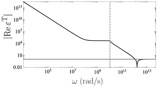
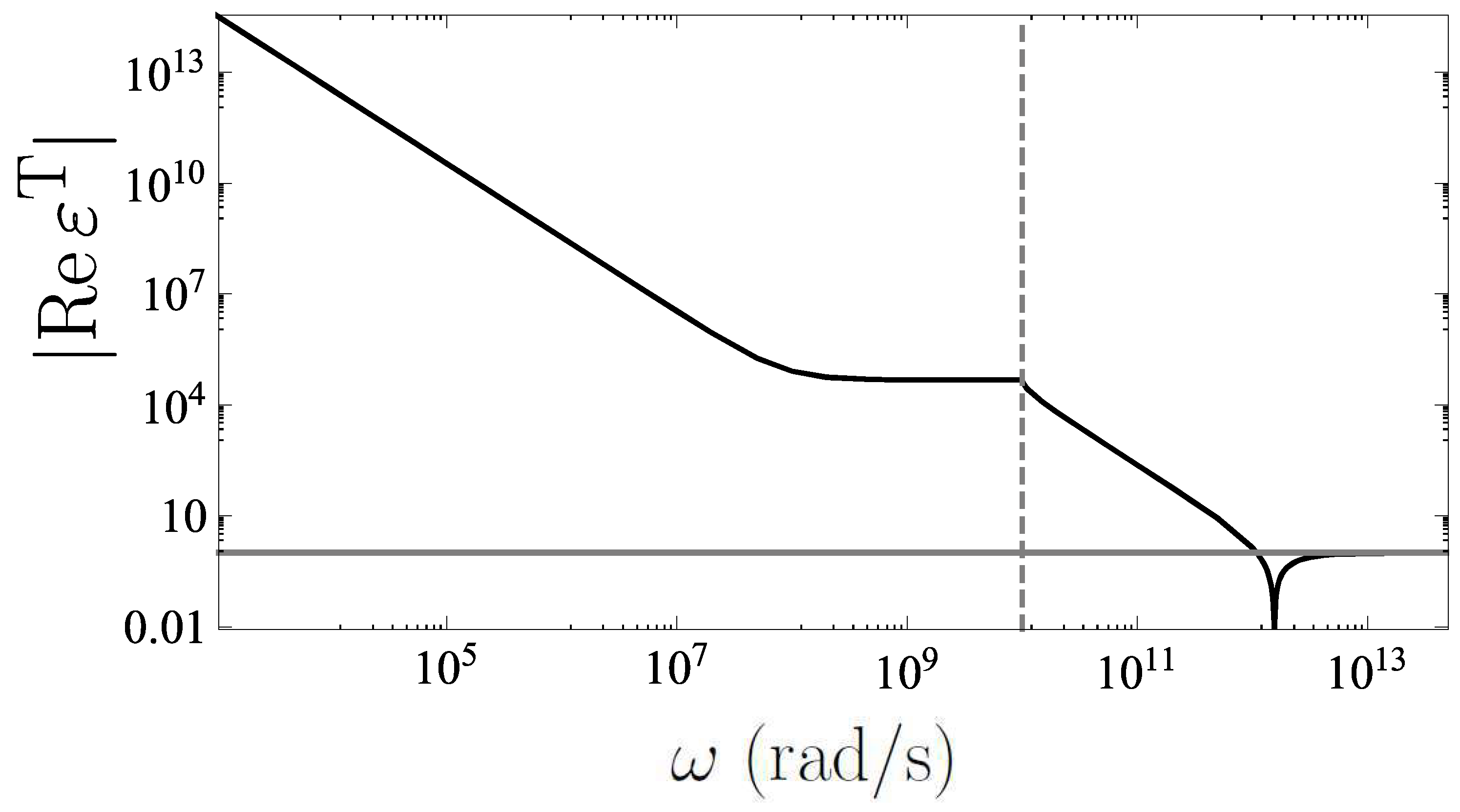
In Figure 3, $|\mathrm{Re}{\epsilon }^{\mathrm{T}}|$ defined by Equation (21) is shown as the function of frequency in the region $\omega <v_{F}q$ for the same values of $T$ and $q$ as in Figure 1 and Figure 2. When $\omega$ approaches $v_{F}q$, $\mathrm{Re}{\epsilon }^{\mathrm{T}}$ approaches the negative constant. The asymptotic expression (26) is well applicable at all $\omega <v_{F}q$.

Figure 3. The magnitude of the real part (21) of the transverse dielectric function of graphene versus frequency for $T=300$ K and $q=100{\mathrm{cm}}^{-1}$. The threshold at $\omega =v_{F}q$ is shown by a dashed vertical line.

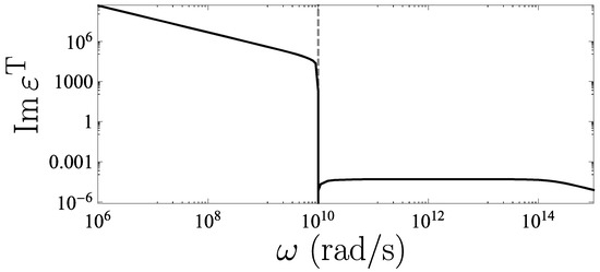
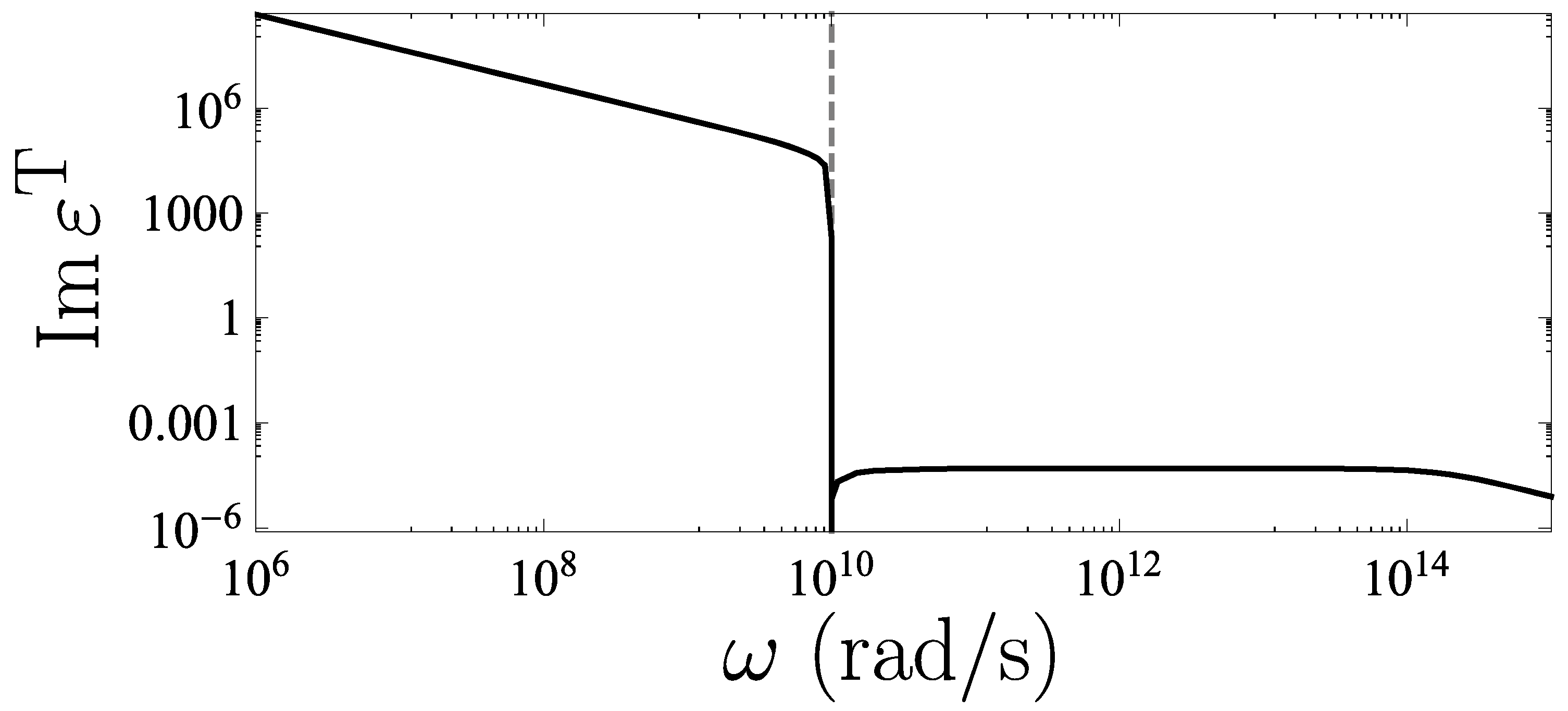
Figure 4 shows the imaginary part $\mathrm{Im}{\epsilon }^{\mathrm{T}}$ (22) of the transverse response function of graphene at $T=300$ K and $q=100{\mathrm{cm}}^{-1}$ as the function of frequency in the region to the left of the vertical line $\omega =v_{F}q$. As is seen in Figure 4, $\mathrm{Im}{\epsilon }^{\mathrm{T}}$ goes to zero when $\omega$ approaches $v_{F}q$ from the left. The asymptotic expression (30) is well applicable for $\omega <2\times {10}^9$ rad/s.

Figure 4. The imaginary part (22) of the transverse dielectric function of graphene versus frequency for $T=300$ K and $q=100{\mathrm{cm}}^{-1}$. The threshold at $\omega =v_{F}q$ is shown by the dashed vertical line.

As opposed to Equation (20) for ${\epsilon }^{\mathrm{L}}$, where one can consider the limit of zero $T$, Equations (26) and (30) for ${\epsilon }^{\mathrm{T}}$ are obtained under a condition $T\ne 0$. The exact expressions for ${\epsilon }^{\mathrm{T}}$ for any $\omega$ at $T=0$ are [99]

$$\mathrm{Im}{\epsilon }^{\mathrm{T}}(\omega ,\mathit{q})=\left\{\begin{array}{cc}-{\displaystyle \frac{\pi \alpha \mathit{qc}}{{\omega }^2}}\sqrt{v_F^2{q}^2-{\omega }^2},& \omega <v_{F}q,\hfill \\ i{\displaystyle \frac{\pi \alpha \mathit{qc}}{2{\omega }^2}}\sqrt{{\omega }^2-v_F^2{q}^2},& \omega >v_{F}q.\hfill \end{array}\right.$$

(31)

Thus, at zero temperature the double pole at zero frequency in ${\epsilon }^{\mathrm{T}}$ is preserved. Note that for graphene the limiting transitions of $\omega$ and $T$ to zero are not interchangeable.

4. Dielectric Functions of Graphene at High Frequencies

Now, we consider the longitudinal and transverse dielectric functions of graphene at all frequencies, satisfying the condition $\omega >v_{F}q$. This includes the region of evanescent waves $v_{F}q<\omega <\mathit{cq}$ and the region of propagating waves $\omega ⩾\mathit{cq}$.

The real and imaginary parts of the longitudinal dielectric function are obtained by substituting Equations (7) and (8) in the first equality of Equation (16):

$$\begin{array}{ccc}& & \mathrm{Re}{\epsilon }^{\mathrm{L}}(\omega ,\mathit{q})=1+{\displaystyle \frac{2\alpha c}{v_F^{2}q}}\left\{\phantom{\left[\underset{0}{\overset{v_{F}q-\omega }{\int }}{\displaystyle \frac{\mathit{dx}}{e^{\beta x}+1}}\right]}{\displaystyle \frac{2\ln 2}{\beta }}\right.-{\displaystyle \frac{1}{\sqrt{{\omega }^2-v_F^2{q}^2}}}\hfill \\ & & \left.\times \left[\underset{0}{\overset{\infty }{\int }}{\displaystyle \frac{\mathit{dx}}{e^{\beta x}+1}}{F}_3\left(x\right)-\underset{\omega +v_{F}q}{\overset{\infty }{\int }}{\displaystyle \frac{\mathit{dx}}{e^{\beta x}+1}}{F}_4\left(x\right)+\underset{0}{\overset{v_{F}q-\omega }{\int }}{\displaystyle \frac{\mathit{dx}}{e^{\beta x}+1}}{F}_4\left(x\right)\right]\right\}\hfill \end{array}$$

(32)

and

$$\mathrm{Im}{\epsilon }^{\mathrm{L}}(\omega ,\mathit{q})={\displaystyle \frac{\alpha c}{2q\sqrt{{\omega }^2-v_F^2{q}^2}}}\left[\pi q^2-{\displaystyle \frac{4}{v_F^2}}\underset{-v_{F}q}{\overset{v_{F}q}{\int }}\mathit{dx}{\displaystyle \frac{\sqrt{v_F^2{q}^2-x^2}}{e^{\beta (\omega +x)}+1}}\right].$$

(33)

Let us consider first the limiting value of $\mathrm{Re}{\epsilon }^{\mathrm{L}}$ (32) when $\omega \to \infty$. By introducing the new integration variable $y=x-\omega$ in the second integral of Equation (32), one obtains

$$-\underset{\omega +v_{F}q}{\overset{\infty }{\int }}{\displaystyle \frac{\mathit{dx}}{e^{\beta x}+1}}{F}_4\left(x\right)=-\underset{v_{F}q}{\overset{\infty }{\int }}{\displaystyle \frac{\mathit{dy}}{e^{\beta (\omega +y)}+1}}\sqrt{y^2-v_F^2{q}^2},$$

(34)

which goes to zero exponentially fast when $\omega \to \infty$ and can be omitted. In the remaining terms in the curly brackets of Equation (32), we change the integration variable according to $x=\omega y$, introduce the small parameter $\delta =v_{F}q/\omega$, and in the limit $\omega \to \infty$, obtain

$$\begin{array}{ccc}& & {\displaystyle \frac{2\ln 2}{\beta }}-{\displaystyle \frac{1}{\sqrt{{\omega }^2-v_F^2{q}^2}}}\underset{0}{\overset{\infty }{\int }}{\displaystyle \frac{\mathit{dx}}{e^{\beta x}+1}}[F_3\left(x\right)+F_4\left(x\right)]\hfill \\ & & ={\displaystyle \frac{2\ln 2}{\beta }}-{\displaystyle \frac{\omega }{\sqrt{1-{\delta }^2}}}\underset{0}{\overset{\infty }{\int }}\mathit{dy}{\displaystyle \frac{\sqrt{{(y+1)}^2-{\delta }^2}+\sqrt{{(y-1)}^2-{\delta }^2}}{e^{\beta \omega y}+1}}={\displaystyle \frac{2\ln 2}{\beta }}-2\omega \underset{0}{\overset{\infty }{\int }}{\displaystyle \frac{\mathit{dy}}{e^{\beta \omega y}+1}}=0.\hfill \end{array}$$

(35)

In Equation (35), it is taken into account that when $\omega \to \infty$, $\beta \omega \gg 1$ holds as well. As a result, the dominant contribution to the integrals is given by $y\ll 1$, so that ${(y+1)}^2\approx {(y-1)}^2\approx 1$, and the square roots can be expanded in powers of the small parameter ${\delta }^2$. Thus, in the limiting case $\omega \to \infty$, one obtains

$$\underset{\omega \to \infty }{\lim }\mathrm{Re}{\epsilon }^{\mathrm{L}}(\omega ,\mathit{q})=1,\underset{\omega \to \infty }{\lim }\mathrm{Im}{\epsilon }^{\mathrm{L}}(\omega ,\mathit{q})=0.$$

(36)

The second equality in Equation (36) is straightforward consequence of Equation (33).

From Equation (33), it also follows that $\mathrm{Im}{\epsilon }^{\mathrm{L}}>0$. The point is that the integrand in Equation (33) is the decreasing function of $\beta$. That is, this integrand takes the maximum value for $\beta =0$ (i.e., for $T=\infty$). Then, one finds

$$\max \underset{-v_{F}q}{\overset{v_{F}q}{\int }}\mathit{dx}{\displaystyle \frac{\sqrt{v_F^2{q}^2-x^2}}{e^{\beta (\omega +x)}+1}}={\displaystyle \frac{1}{2}}\underset{-v_{F}q}{\overset{v_{F}q}{\int }}\mathit{dx}\sqrt{v_F^2{q}^2-x^2}={\displaystyle \frac{\pi }{4}}{v}_F^2{q}^2.$$

(37)

Substituting Equation (37) into Equation (33), one finds that $\min \left(\mathrm{Im}{\epsilon }^{\mathrm{L}}\right)=0$ and conclude that for all $T<\infty$ holds $\mathrm{Im}{\epsilon }^{\mathrm{L}}>0$.

In Figure 1 and Figure 2, in the domains to the right of the dashed vertical lines ($\omega >v_{F}q$), the quantities $|\mathrm{Re}{\epsilon }^{\mathrm{L}}|$ (32) and $\mathrm{Im}{\epsilon }^{\mathrm{L}}$ (33), respectively, are shown as the functions of frequency. When $\omega$ increases from $v_{F}q$ to $1.54\times {10}^{12}$, $\mathrm{Re}{\epsilon }^{\mathrm{L}}$ varies from $-\infty$ to 0. With a further increase of $\omega$, $\mathrm{Re}{\epsilon }^{\mathrm{L}}$ changes its sign and increases to unity shown by the gray line in Figure 1. Regarding $\mathrm{Im}{\epsilon }^{\mathrm{L}}$, one sees that it abruptly drops to 0 for $\omega >v_{F}q$.

The real and imaginary parts of the transverse dielectric function of graphene under the condition $\omega >v_{F}q$ are found from Equations (9) and (10) and the second equality of Equation (16):

$$\begin{array}{ccc}& & \mathrm{Re}{\epsilon }^{\mathrm{T}}(\omega ,\mathit{q})=1-{\displaystyle \frac{2\alpha c}{v_F^{2}q}}\left\{\phantom{\left[\underset{0}{\overset{v_{F}q-\omega }{\int }}{\displaystyle \frac{\mathit{dx}}{e^{\beta x}+1}}\right]}{\displaystyle \frac{2\ln 2}{\beta }}\right.-{\displaystyle \frac{\sqrt{{\omega }^2-v_F^2{q}^2}}{{\omega }^2}}\hfill \\ & & \times \left[\underset{0}{\overset{\infty }{\int }}{\displaystyle \frac{\mathit{dx}}{e^{\beta x}+1}}{\displaystyle \frac{{(x+\omega )}^2}{F_3\left(x\right)}}-\underset{\omega +v_{F}q}{\overset{\infty }{\int }}{\displaystyle \frac{\mathit{dx}}{e^{\beta x}+1}}{\displaystyle \frac{{(x-\omega )}^2}{F_4\left(x\right)}}\right.\left.\left.+\underset{0}{\overset{v_{F}q-\omega }{\int }}{\displaystyle \frac{\mathit{dx}}{e^{\beta x}+1}}{\displaystyle \frac{{(x-\omega )}^2}{F_4\left(x\right)}}\right]\right\}\hfill \end{array}$$

(38)

and

$$\mathrm{Im}{\epsilon }^{\mathrm{T}}(\omega ,\mathit{q})={\displaystyle \frac{\alpha c}{2v_F^{2}q{\omega }^2}}\sqrt{{\omega }^2-v_F^2{q}^2}\left[\pi v_F^2{q}^2-4\underset{-v_{F}q}{\overset{v_{F}q}{\int }}{\displaystyle \frac{\mathit{dx}}{e^{\beta (\omega +x)}+1}}{\displaystyle \frac{x^2}{\sqrt{v_F^2{q}^2-x^2}}}\right].$$

(39)

Let us consider first $\mathrm{Re}{\epsilon }^{\mathrm{T}}$ in the limiting case $\omega \to \infty$. The second integral on the r.h.s. of Equation (38) vanishes and the remaining two integrals can be rearranged to

$$\begin{array}{ccc}& & -{\displaystyle \frac{\sqrt{{\omega }^2-v_F^2{q}^2}}{{\omega }^2}}\underset{0}{\overset{\infty }{\int }}{\displaystyle \frac{\mathit{dx}}{e^{\beta x}+1}}\left[{\displaystyle \frac{{(x+\omega )}^2}{F_3\left(x\right)}}+{\displaystyle \frac{{(x-\omega )}^2}{F_4\left(x\right)}}\right]\hfill \\ & & =-{\displaystyle \frac{\sqrt{{\omega }^2-v_F^2{q}^2}}{{\omega }^2}}\underset{0}{\overset{\infty }{\int }}{\displaystyle \frac{\mathit{dx}}{e^{\beta x}+1}}\left[F_3\left(x\right)+{\displaystyle \frac{v_F^2{q}^2}{F_3\left(x\right)}}+F_4\left(x\right)+{\displaystyle \frac{v_F^2{q}^2}{F_4\left(x\right)}}\right]\hfill \\ & & \approx -{\displaystyle \frac{\omega }{{\omega }^2}}\underset{0}{\overset{\infty }{\int }}{\displaystyle \frac{\mathit{dx}}{e^{\beta x}+1}}(\omega +\omega )=-2\underset{0}{\overset{\infty }{\int }}{\displaystyle \frac{\mathit{dx}}{e^{\beta x}+1}}=-{\displaystyle \frac{2\ln 2}{\beta }}.\hfill \end{array}$$

(40)

That is, the first term in the curly brackets of Equation (38) is canceled by Equation (40) and one obtains

$$\underset{\omega \to \infty }{\lim }\mathrm{Re}{\epsilon }^{\mathrm{T}}(\omega ,\mathit{q})=1,\underset{\omega \to \infty }{\lim }\mathrm{Im}{\epsilon }^{\mathrm{T}}(\omega ,\mathit{q})=0$$

(41)

(the latter limit is straightforward from Equation (39)).

From Equation (39), it is also seen that $\mathrm{Im}{\epsilon }^{\mathrm{T}}>0$. This is because the maximum value of the subtracted integral is reached at $\beta =0$ ($T=\infty$), similar to that in Equation (33). That is, the integral in Equation (39) is

$$\max \underset{-v_{F}q}{\overset{v_{F}q}{\int }}{\displaystyle \frac{x^2\mathit{dx}}{(e^{\beta (\omega +x)}+1)\sqrt{v_F^2{q}^2-x^2}}}={\displaystyle \frac{1}{2}}\underset{-v_{F}q}{\overset{v_{F}q}{\int }}{\displaystyle \frac{x^2\mathit{dx}}{\sqrt{v_F^2{q}^2-x^2}}}={\displaystyle \frac{\pi }{4}}{v}_F^2{q}^2,$$

(42)

which cancels the first term. Thus, at any $T<\infty$, the inequality $\mathrm{Im}{\epsilon }^{\mathrm{T}}>0$ holds.

In Figure 3 and Figure 4, in the region $\omega >v_{F}q$, the quantities $|\mathrm{Re}{\epsilon }^{\mathrm{T}}|$ (38) and $\mathrm{Im}{\epsilon }^{\mathrm{T}}$ (39), respectively, are shown as the functions of frequency. When $\omega$ increases from $v_{F}q$ to $1.52\times {10}^{12}$ rad/s, $\mathrm{Re}{\epsilon }^{\mathrm{T}}$ goes to 0, remaining negative, and then changes its sign and goes to unity shown by the gray line in Figure 3. For $\omega >v_{F}q$, $\mathrm{Im}{\epsilon }^{\mathrm{T}}$ first increases from 0 and then decreases to 0 at $\omega =\infty$. Figure 1, Figure 2, Figure 3 and Figure 4 demonstrate the presence of a threshold at $\omega =v_{F}q$ [85,99].

At $T=0$, below the threshold, $\mathrm{Re}{\epsilon }^{\mathrm{L},\mathrm{T}}$ are given by the first two terms in Equations (18) and (21), whereas $\mathrm{Im}{\epsilon }^{\mathrm{L},\mathrm{T}}=0$. Above the threshold, b $\mathrm{Re}{\epsilon }^{\mathrm{L},\mathrm{T}}=1$ and $\mathrm{Im}{\epsilon }^{\mathrm{L},\mathrm{T}}$ are given by the first terms in Equations (33) and (39). In each case, an order in the limiting transitions of $\omega$ and $q$ to 0 is fixed. At the point of threshold, the derivatives become discontinuous.

The dielectric functions of graphene expressed via the polarization tensor are, by construction, analytic in the upper half-plane of complex frequency and thus satisfy the Kramers–Kronig relations. The permittivity ${\epsilon }^{\mathrm{L}}$ is regular at zero frequency and satisfies the standard Kramers–Kronig relations that are valid for dielectric materials [53], but has a threshold at $\omega =v_{F}q$. Regarding the permittivity ${\epsilon }^{\mathrm{T}}$, it is of the most nonconventional character because, according to Equations (26) and (30), at nonzero temperature both the real and imaginary parts of ${\epsilon }^{\mathrm{T}}$ have a single pole at $\omega =0$, whereas $\mathrm{Re}{\epsilon }^{\mathrm{T}}$ also has the double pole. As noted above, both Equations (26) and (30) are obtained under the condition $T\ne 0$ and it is not possible to consider the limit of zero temperature in these expressions. At $T=0$, there is no single pole in ${\epsilon }^{\mathrm{T}}$ [99].

The presence of a single pole, like that in the imaginary part of the dielectric permittivity of the Drude model, gives rise to the known additional term in the Kramers–Kronig relations [53]. A similar term appears in the case of a double pole (see Ref. [99] for details). In Ref. [99], it is also shown that the branch points that are present in both ${\epsilon }^{\mathrm{L}}$ and ${\epsilon }^{\mathrm{T}}$ at $\omega =v_{F}q$ do not affect the form of the Kramers–Kronig relations.

As noted in Section 1, all derivations in this study are made for the case of pristine graphene possessing a zero mass gap parameter $\Delta =2{\mathit{mv}}_F^2$, with $m$ the quasiparticle mass, and zero chemical potential $\mu$. In the case when $\Delta$ and $\mu$ are not equal to 0, the low-frequency behavior of the dielectric functions of graphene depends on the values of $\Delta$ and $\mu$ and preserves the same pole structure as for a pristine graphene. Using expressions for the polarization tensor with the arbitrary values of $\Delta$ and $\mu$ (see, for instance, Ref. [74]), one can find that if $\Delta$, $\mu$ and $\omega$ simultaneously go to 0, one returns to Equations (20), (26) and (30) independently of the order of limiting transitions.

5. Discussion

In this paper, we investigated the dependence of the dielectric functions of graphene on frequency. The most intriguing unusual analytic properties were found for the real part of the transverse function, ${\epsilon }^{\mathrm{T}}$, at low frequencies. Thus, both the real and imaginary parts of ${\epsilon }^{\mathrm{T}}$ possess the single pole at zero frequency. What is more, the spatially nonlocal term in its real part also possesses the double pole, which is not the case for conventional materials according to present views. The double pole should be also present in the response functions of other two-dimensional Dirac materials such as germanene [100,101,102], silicene [103,104,105], phosphorene [106,107,108], and stanene [109,110,111]. In spite of the presence of a double pole, the dielectric functions of graphene satisfy all the necessary physical demands. These dielectric functions possess positive imaginary parts, which describe dissipation on the basis of first principles, and satisfy the Kramers–Kronig relations expressing the condition of causality. Because of this, an attempt [84] to modify the polarization tensor in order to remove the double pole predicted by the first principles of quantum field theory is unjustified.

There is also a long-standing problem called the Casimir puzzle. To bring the theoretical predictions of the fundamental Lifshitz theory in agreement with the measurement data, the dielectric response of metals at low frequencies was described by the plasma model possessing the double pole at $\omega =0$ (see Refs. [112,113,114,115] for a review). However, as remarked above, this model is applicable only at high enough frequencies. That is why an example of graphene, whose dielectric function possessing the double pole at zero frequency is derived starting from first physical principles and leads to agreement with measurements of the Casimir force, may pave the way for resolution of the Casimir puzzle.

6. Conclusions

In the foregoing, we listed several phenomenological theoretical approaches used for investigation of the dielectric response of graphene. It is underlined that at the characteristic energies below approximately 3 eV, the spatially nonlocal response functions of graphene can be derived within the Dirac model starting from the first principles of thermal quantum field theory. The obtained dielectric functions are instructive for a theoretical description of a number of physical phenomena in graphene systems, such as the Casimir and Casimir–Polder forces both in equilibrium situations and out of thermal equilibrium, radiative heat transfer, atomic friction, surface plasmons, and others.

According to the results obtained here, these functions possess all the properties necessary for the dielectric functions and their transverse part has the double pole at zero frequency at any nonzero wave vector. The above discussion allows to conjecture that the spatially nonlocal transverse electric response function of metals possesses the double pole in the region of evanescent waves, as holds for graphene. Recently, it was demonstrated [116] that the predictions of classical electrodynamics using the Drude dielectric function for the field of oscillating magnetic dipole reflected from a copper plate, which is fully determined by the transverse electric evanescent waves, are in contradiction with the measurements. Future progress in the investigation of such physical phenomena as the Casimir effect, atomic friction, radiative heat transfer, near-field optical microscopy, total internal reflection, and frustrated total internal reflection is closely aligned with the resolution of this problem.

References

- Planck, M. Zur Theorie des Gesetzes der Energieverteilung im Normalspectrum. Verhandl. Deutsch. Phys. Gesllsch. 1900, 2, 237–245, English translation: On the theory of the energy distribution law of the normal spectrum. In ter Haar, D. The Old Quantum Theory; Pergamon Press Ltd.: Oxford, UK, 1967; pp. 82–89. Available online: https://archive.org/details/oldquantumtheory00haar (accessed on 13 January 2025).
- Einstein, A. Über einen die Erzeugung und Verwandlung des Lichtes betreffenden heuristischen Gesichtspunkt. Ann. d. Phys. 1905, 17, 132–148, English translation: On a heuristic point of view about the creation and conversion of light. In ter Haar, D. The Old Quantum Theory; Pergamon Press Ltd.: Oxford, UK, 1967; pp. 91–107. Available online: https://archive.org/details/oldquantumtheory00haar (accessed on 13 January 2025).
- Heisenberg, W. Über quantentheoretische Umdeutung kinematischer und mechanischer Beziehungen. Z. Phys. 1925, 33, 879–893, English translation: Quantum-theoretical reinterpretation of kinematic and mechanical relations. In Sources of Quantum Mechanics; van derWaerden, B.L., Ed.; North-Holland Publishing Co.: Amsterdam, The Netherlands; Dover Publications, Inc.: New York, NY, USA, 1967; pp. 261–276. Available online: https://archive.org/details/sourcesofquantum0000unse (accessed on 13 January 2025).
- Schrödinger, E. An undulatory theory of the mechanics of atoms and molecules. Phys. Rev. 1926, 28, 1049–1070. [Google Scholar] [CrossRef] [Scilit]
- Dirac, P.A.M. The Quantum Theory of the Electron. Proc. R. Soc. A Math. Phys. Eng. Sci. 1928, 117, 610–624. [Google Scholar] [CrossRef] [Scilit]
- Castro Neto, A.H.; Guinea, F.; Peres, N.M.R.; Novoselov, K.S.; Geim, A.K. The electronic properties of graphene. Rev. Mod. Phys. 2009, 81, 109–162. [Google Scholar] [CrossRef] [Scilit]
- Aoki, H.; Dresselhaus, M.S. (Eds.) Physics of Graphene; Springer International Publishing Switzerland: Cham, Switzerland, 2014. [Google Scholar] [CrossRef] [Scilit]
- Katsnelson, M.I. The Physics of Graphene; Cambridge University Press: Cambridge, UK, 2020. [Google Scholar] [CrossRef] [Scilit]
- Sernelius, B.E. Retarded interactions in graphene systems. Phys. Rev. B 2012, 85, 195427. [Google Scholar] [CrossRef] [Scilit]
- Sernelius, B.E. Fundamentals of van der Waals and Casimir Interactions; Springer Nature Switzerland AG: Cham, Switzerland, 2018. [Google Scholar] [CrossRef] [Scilit]
- Barton, G. Casimir energies of spherical plasma shells. J. Phys. A Math. Gen. 2004, 37, 1011–1050. [Google Scholar] [CrossRef] [Scilit]
- Barton, G. Casimir effect for a flat plasma sheet. I. Energies. J. Phys. A Math. Gen. 2005, 38, 2997–3020. [Google Scholar] [CrossRef] [Scilit]
- Bordag, M. The Casimir effect for thin plasma sheets and the role of the surface plasmons. J. Phys. A Math. Gen. 2006, 39, 6173–6185. [Google Scholar] [CrossRef] [Scilit]
- Peres, N.M.R.; Lopes dos Santos, J.M.B.; Stauber, T. Phenomenological study of the electronic transport coefficients of graphene. Phys. Rev. B 2007, 76, 073412. [Google Scholar] [CrossRef] [Scilit]
- Vasko, F.T.; Ryzhii, V. Voltage and temperature dependencies of conductivity in gated graphene. Phys. Rev. B 2007, 76, 233404. [Google Scholar] [CrossRef] [Scilit]
- Falkovsky, L.A.; Pershoguba, S.S. Optical far-infrared properties of a graphene monolayer and multilayer. Phys. Rev. B 2007, 76, 153410. [Google Scholar] [CrossRef] [Scilit]
- Stauber, T.; Peres, N.M.R.; Guinea, F. Electronic transport in graphene: A semiclassical approach including midgap states. Phys. Rev. B 2007, 76, 205423. [Google Scholar] [CrossRef] [Scilit]
- Falkovsky, L.A.; Varlamov, A.A. Space-time dispersion of graphene conductivity. Eur. Phys. J. B 2007, 56, 281–284. [Google Scholar] [CrossRef] [Scilit]
- Falkovsky, L.A. Optical properties of graphene. J. Phys. Conf. Ser. 2008, 129, 012004. [Google Scholar] [CrossRef] [Scilit]
- Moriconi, L.; Niemeyer, D. Graphene conductivity near the charge neutral point. Phys. Rev. B 2011, 84, 193401. [Google Scholar] [CrossRef] [Scilit]
- Horng, J.; Chen, C.-F.; Geng, B.; Girit, C.; Zhang, Y.; Hao, Z.; Bechtel, H.A.; Martin, M.; Zettl, A.; Crommie, M.F.; et al. Drude conductivity of Dirac fermions in graphene. Phys. Rev. B 2011, 83, 165113. [Google Scholar] [CrossRef] [Scilit]
- Patel, D.K.; Sharma, A.C.; Ashraf, S.S.Z. Temperature dependent screened electronic transport in gapped graphene. Phys. Status Solidi 2015, 252, 282. [Google Scholar] [CrossRef] [Scilit]
- Wunsch, B.; Stauber, T.; Sols, F.; Guinea, F. Dynamical polarization of graphene at finite doping. New J. Phys. 2006, 8, 318. [Google Scholar] [CrossRef] [Scilit]
- Gusynin, V.P.; Sharapov, S.G.; Carbotte, J.P. Anomalous absorption line in the magneto-optical response of graphene. Phys. Rev. Lett. 2007, 98, 157402. [Google Scholar] [CrossRef] [Scilit]
- Hwang, E.H.; Das Sarma, S. Dielectric function, screening, and plasmons in two-dimensional graphene. Phys. Rev. B 2007, 75, 205418. [Google Scholar] [CrossRef] [Scilit]
- Qaiumzadeh, A.; Asgari, R. Ground-state properties of gapped graphene using the random phase approximation. Phys. Rev. B 2009, 79, 075414. [Google Scholar] [CrossRef] [Scilit]
- Gómez-Santos, G. Thermal van der Waals interaction between graphene layers. Phys. Rev. B 2009, 80, 245424. [Google Scholar] [CrossRef] [Scilit]
- Scholz, A.; Schliemann, J. Dynamical current-current susceptibility of gapped graphene. Phys. Rev. B 2011, 83, 235409. [Google Scholar] [CrossRef] [Scilit]
- Koppens, F.H.L.; Chang, D.E.; García de Abajo, F.J. Graphene plasmonics: A platform for strong light-matter interactions. Nano Lett. 2011, 11, 3370. [Google Scholar] [CrossRef] [Scilit] [PubMed]
- Svetovoy, V.; Moktadir, Z.; Elwenspoek, M.; Mizuta, H. Tailoring the thermal Casimir force with graphene. EPL (Europhys. Lett.) 2011, 96, 14006. [Google Scholar] [CrossRef] [Scilit]
- Sarabadani, J.; Naji, A.; Asgari, R.; Podgornik, R. Many-body effects in the van der Waals–Casimir interaction between graphene layers. Phys. Rev. B 2011, 84, 155407. [Google Scholar] [CrossRef] [Scilit]
- Gutiérrez-Rubio, A.; Stauber, T.; Guinea, F. Transverse current response of graphene at finite temperature: Plasmons and absorption. J. Opt. 2013, 15, 114005. [Google Scholar] [CrossRef] [Scilit]
- Palacios, J.J. Origin of the quasiuniversality of the minimal conductivity of graphene. Phys. Rev. B 2010, 82, 165439. [Google Scholar] [CrossRef] [Scilit]
- Rani, P.; Dubey, G.S.; Jindal, V.K. DFT study of optical properties of pure and doped graphene. Phys. E 2014, 62, 28–35. [Google Scholar] [CrossRef] [Scilit]
- Gusynin, V.P.; Sharapov, S.G. Transport of Dirac quasiparticles in graphene: Hall and optical conductivities. Phys. Rev. B 2006, 73, 245411. [Google Scholar] [CrossRef] [Scilit]
- Katsnelson, M.I. Zitterbewegung, chirality, and minimal conductivity in graphene. Eur. Phys. J. B 2006, 51, 157–160. [Google Scholar]
- Peres, N.M.R.; Guinea, F.; Castro Neto, A.H. Electronic properties of disordered two-dimensional carbon. Phys. Rev. B 2006, 73, 125411. [Google Scholar] [CrossRef] [Scilit]
- Tworzydło, J.; Trauzettel, B.; Titov, M.; Rycerz, A.; Beenakker, C.W.J. Sub-Poissonian shot noise in graphene. Phys. Rev. Lett. 2006, 96, 246802. [Google Scholar] [CrossRef] [Scilit] [PubMed]
- Ziegler, K. Robust transport properties in graphene. Phys. Rev. Lett. 2006, 97, 266802. [Google Scholar] [CrossRef] [Scilit] [PubMed]
- Ziegler, K. Minimal conductivity of graphene: Nonuniversal values from the Kubo formula. Phys. Rev. B 2007, 75, 233407. [Google Scholar] [CrossRef] [Scilit]
- Stauber, T.; Peres, N.M.R.; Geim, A.K. Optical conductivity of graphene in the visible region of the spectrum. Phys. Rev. B 2008, 78, 085432. [Google Scholar] [CrossRef] [Scilit]
- Peres, N.M.R.; Stauber, T. Transport in a clean graphene sheet at finite temperature and frequency. Int. J. Mod. Phys. B 2008, 22, 2529–2536. [Google Scholar] [CrossRef] [Scilit]
- Buividovich, P.V.; Luschevskaya, E.V.; Pavlovsky, O.V.; Polikarpov, M.I.; Ulybyshev, M.V. Numerical study of the conductivity of graphene monolayer within the effective field theory approach. Phys. Rev. B 2012, 86, 045107. [Google Scholar] [CrossRef] [Scilit]
- Drosdoff, D.; Phan, A.D.; Woods, L.M.; Bondarev, I.V.; Dobson, J.F. Effects of spatial dispersion on the Casimir force between graphene sheets. Eur. Phys. J. B 2012, 85, 365. [Google Scholar] [CrossRef] [Scilit]
- Bácsi, Á.; Virosztek, A. Low-frequency optical conductivity in graphene and in other scale-invariant two-band systems. Phys. Rev. B 2013, 87, 125425. [Google Scholar] [CrossRef] [Scilit]
- Dartora, C.A.; Cabrera, G.G. U(1)×SU(2) gauge invariance leading to charge and spin conductivity of Dirac fermions in graphene. Phys. Rev. B 2013, 87, 165416. [Google Scholar] [CrossRef] [Scilit]
- Drosdoff, D.; Woods, L.M. Casimir forces and graphene sheets. Phys. Rev. B 2010, 82, 155459. [Google Scholar] [CrossRef] [Scilit]
- Merano, M. Fresnel coefficients of a two-dimensional atomic crystal. Phys. Rev. A 2016, 93, 013832. [Google Scholar] [CrossRef] [Scilit]
- Gusynin, V.P.; Sharapov, S.G.; Carbotte, J.P. AC conductivity of graphene: From tight-binding model to 2+1-dimensional quantum electrodynamics. Int. J. Mod. Phys. B 2007, 21, 4611–4658. [Google Scholar] [CrossRef] [Scilit]
- Peres, N.M.R. The transport properties of graphene: An introduction. Rev. Mod. Phys. 2010, 82, 2673–2700. [Google Scholar] [CrossRef] [Scilit]
- Das Sarma, S.; Adam, S.; Hwang, E.H.; Rossi, E. Electronic transport in two-dimensional graphene. Rev. Mod. Phys. 2011, 83, 407–470. [Google Scholar] [CrossRef] [Scilit]
- Klimchitskaya, G.L.; Mostepanenko, V.M. Temperature dependence of the response functions of graphene: Impact on Casimir and Casimir–Polder forces in and out of thermal equilibrium. Physics 2025, 7, 44. [Google Scholar] [CrossRef] [Scilit]
- Landau, L.D.; Lifshitz, E.M.; Pitaevskii, L.P. Electrodynamics of Continuous Media; Pergamon Press Ltd.: Oxford, UK; Elsevier Ltd.: Oxford, UK, 1984; Available online: https://www.sciencedirect.com/book/monograph/9780080302751/electrodynamics-of-continuous-media (accessed on 13 January 2025).
- Pisarski, R.D. Chiral symmetry breaking in three-dimensional electrodynamics. Phys. Rev. D 1984, 29, 2423–2426. [Google Scholar] [CrossRef] [Scilit]
- Appelquist, T.W.; Bowick, M.J.; Karabali, D.; Wijewardhana, L.C.R. Spontaneous chiral-symmetry breaking in three-dimensional QED. Phys. Rev. D 1986, 33, 3704–3713. [Google Scholar] [CrossRef] [Scilit]
- Gorbar, E.V.; Gusynin, V.P.; Miransky, V.A.; Shovkovy, I.A. Magnetic field driven metal-insulator phase transition in planar systems. Phys. Rev. B 2002, 66, 045108. [Google Scholar] [CrossRef] [Scilit]
- Pyatkovsky, P.K. Dynamical polarization, screening, and plasmons in gapped graphene. J. Phys. Condens. Matter 2009, 21, 025506. [Google Scholar] [CrossRef] [Scilit]
- Bordag, M.; Fialkovsky, I.V.; Gitman, D.M.; Vassilevich, D.V. Casimir interaction between a perfect conductor and graphene described by the Dirac model. Phys. Rev. B 2009, 80, 245406. [Google Scholar] [CrossRef] [Scilit]
- Li, W.; Liu, G.-Z. Dynamical chiral symmetry breaking in QED3 at finite density and impurity potential. Phys. Rev. D 2010, 81, 045006. [Google Scholar] [CrossRef] [Scilit]
- Fialkovsky, I.V.; Marachevsky, V.N.; Vassilevich, D.V. Finite-temperature Casimir effect for graphene. Phys. Rev. B 2011, 84, 035446. [Google Scholar] [CrossRef] [Scilit]
- Bordag, M.; Klimchitskaya, G.L.; Mostepanenko, V.M.; Petrov, V.M. Quantum field theoretical description for the reflectivity of graphene. Phys. Rev. D 2015, 91, 045037. [Google Scholar] [CrossRef] [Scilit]
- Bordag, M.; Fialkovskiy, I.; Vassilevich, D. Enhanced Casimir effect for doped graphene. Phys. Rev. B 2016, 93, 075414. [Google Scholar] [CrossRef] [Scilit]
- Klimchitskaya, G.L.; Mostepanenko, V.M. Conductivity of pure graphene: Theoretical approach using the polarization tensor. Phys. Rev. B 2016, 93, 245419. [Google Scholar] [CrossRef] [Scilit]
- Klimchitskaya, G.L.; Mostepanenko, V.M. Quantum electrodynamic approach to the conductivity of gapped graphene. Phys. Rev. B 2016, 94, 195405. [Google Scholar] [CrossRef] [Scilit]
- Klimchitskaya, G.L.; Mostepanenko, V.M.; Petrov, V.M. Conductivity of graphene in the framework of Dirac model: Interplay between nonzero mass gap and chemical potential. Phys. Rev. B 2017, 96, 235432. [Google Scholar] [CrossRef] [Scilit]
- Klimchitskaya, G.L.; Mostepanenko, V.M. Kramers–Kronig relations and causality conditions for graphene in the framework of Dirac model. Phys. Rev. D 2018, 97, 085001. [Google Scholar] [CrossRef] [Scilit]
- Klimchitskaya, G.L.; Mostepanenko, V.M. Reflectivity properties of graphene with a nonzero mass-gap parameter. Phys. Rev. A 2016, 93, 052106. [Google Scholar] [CrossRef] [Scilit]
- Klimchitskaya, G.L.; Mostepanenko, V.M. Optical properties of dielectric plates coated with gapped graphene. Phys. Rev. B 2017, 95, 035425. [Google Scholar] [CrossRef] [Scilit]
- Klimchitskaya, G.L.; Mostepanenko, V.M.; Petrov, V.M. Impact of chemical potential on the reflectance of graphene in the infrared and microwave domains. Phys. Rev. A 2018, 98, 023809. [Google Scholar] [CrossRef] [Scilit]
- Klimchitskaya, G.L.; Mostepanenko, V.M.; Tsybin, O.Y. Casimir–Polder attraction and repulsion between nanoparticles and graphene in out-of-thermal-equilibrium conditions. Phys. Rev. B 2022, 105, 195430. [Google Scholar] [CrossRef] [Scilit]
- Klimchitskaya, G.L.; Korikov, C.C.; Mostepanenko, V.M.; Tsybin, O.Y. Impact of mass-gap on the dispersion interaction of nanoparticles with graphene out of thermal equilibrium. Appl. Sci. 2023, 13, 7511. [Google Scholar] [CrossRef] [Scilit]
- Klimchitskaya, G.L.; Korikov, C.C.; Mostepanenko, V.M.; Tsybin, O.Y. Nonequilibrium Casimir–Polder interaction between nanoparticles and substrates coated with gapped graphene. Symmetry 2023, 15, 1580. [Google Scholar] [CrossRef] [Scilit]
- Klimchitskaya, G.L.; Korikov, C.C.; Mostepanenko, V.M. Nonequilibrium Casimir–Polder force between nanoparticles and graphene-coated silica plate: Combined effect of the chemical potential and mass gap. Symmetry 2024, 16, 320. [Google Scholar] [CrossRef] [Scilit]
- Klimchitskaya, G.L.; Korikov, C.C.; Mostepanenko, V.M. Polarization tensor in spacetime of three dimensions and a quantum field-theoretical description of the nonequilibrium Casimir force in graphene systems. Phys. Rev. A 2025, 111, 012812. [Google Scholar] [CrossRef] [Scilit]
- Klimchitskaya, G.L.; Korikov, C.C.; Mostepanenko, V.M. Nonequilibrium Casimir pressure for two graphene-coated plates: Quantum field theoretical approach. Int. J. Mod. Phys. A 2025, 40, 2543003. [Google Scholar] [CrossRef] [Scilit]
- Starke, R.; Schober, G.A.H. Relativistic covariance of Ohms law. Int. J. Mod. Phys. D 2016, 25, 1640010. [Google Scholar] [CrossRef] [Scilit]
- Melrose, D.B. Quantum Plasmadynamics: Unmagnetized Plasmas; Springer Science+Business Media, LLC: New York, NY, USA, 2008. [Google Scholar] [CrossRef] [Scilit]
- Fialkovskiy, I.V.; Vassilevich, D.V. Quantum field theory in graphene. Int. J. Mod. Phys. A 2012, 27, 1260007. [Google Scholar] [CrossRef] [Scilit]
- Bordag, M.; Pirozhenko, I.G. Transverse-electric surface plasmon for graphene in the Dirac equation model. Phys. Rev. B 2014, 89, 035421. [Google Scholar] [CrossRef] [Scilit]
- Fialkovskiy, I.V.; Vassilevich, D.V. Graphene through the looking glass of QFT. Mod. Phys. Lett. A 2016, 31, 1630047. [Google Scholar] [CrossRef] [Scilit]
- Khusnutdinov, N.; Vassilevich, D.V. Impurities in graphene and their influence on the Casimir interaction. Phys. Rev. B 2024, 109, 235420. [Google Scholar] [CrossRef] [Scilit]
- Khusnutdinov, N.; Emelianova, N. The polarization tensor approach for Casimir effect. Int. J. Mod. Phys. A 2025, 40, 2543004. [Google Scholar] [CrossRef] [Scilit]
- Klimchitskaya, G.L.; Mostepanenko, V.M.; Sernelius, B.E. Two approaches for describing the Casimir interaction with graphene: Density-density correlation function versus polarization tensor. Phys. Rev. B 2014, 89, 125407. [Google Scholar] [CrossRef] [Scilit]
- Rodriguez-Lopez, P.; Wang, J.-S.; Antezza, M. Electric conductivity in graphene: Kubo model versus a nonlocal quantum field theory model. Phys. Rev. B 2025, 111, 115428. [Google Scholar] [CrossRef] [Scilit]
- Bordag, M.; Klimchitskaya, G.L.; Mostepanenko, V.M. Convergence of the polarization tensor in spacetime of three dimensions. Phys. Rev. D 2024, 109, 125014. [Google Scholar] [CrossRef] [Scilit]
- Bordag, M.; Khusnutdinov, N.; Klimchitskaya, G.L.; Mostepanenko, V.M. Comment on “Electric conductivity in graphene: Kubo model versus a nonlocal quantum field theory model”. arXiv 2025, to appear in Phys. Rev. B.. arXiv:2506.10792. [Google Scholar] [CrossRef] [Scilit]
- Rickayzen, G. Theory of Superconductivity; John Wiley & Sons, Inc.: New York, NY, USA, 1965; Available online: https://archive.org/details/theoryofsupercon0000rick (accessed on 13 January 2025).
- van der Marel, D.; Habermeier, H.-U.; Heitmann, D.; König, W.; Wittlin, A. Infrared study of the superconducting phase transition in YBa2Cu3O7-x. Phys. C Supercond. 1991, 176, 1–18. [Google Scholar] [CrossRef] [Scilit]
- Zimmermann, W.; Brandt, E.H.; Bauer, M.; Seider, E.; Genzel, L. Optical conductivity of BCS superconductors with arbitrary purity. Phys. C Supercond. 1991, 183, 99–104. [Google Scholar] [CrossRef] [Scilit]
- Berlinsky, A.J.; Kallin, C.; Rose, G.; Shi, A.-C. Two-fluid interpretation of the conductivity of clean BCS superconductors. Phys. Rev. B 1993, 48, 4074–4079. [Google Scholar] [CrossRef] [Scilit] [PubMed]
- Tachiki, M.; Koyama, T.; Takahashi, S. Electromagnetic phenomena related to a low-frequency plasma in cuprate superconductors. Phys. Rev. B 1994, 50, 7065–7084. [Google Scholar] [CrossRef] [Scilit] [PubMed]
- Pokrovsky, S.V.; Pokrovsky, V.L. Plasma resonance in layered normal metals and superconductors. J. Supercond. 1995, 8, 183–200. [Google Scholar] [CrossRef] [Scilit]
- Tinkham, M. Introduction to Superconductivity; McGraw-Hill, Inc.: Singapore, 1996; Available online: https://archive.org/details/introductiontosu0000mich (accessed on 13 January 2025).
- Bimonte, G.; Calloni, E.; Esposito, G.; Milano, L.; Rosa, L. Towards measuring variations of Casimir energy by a superconducting cavity. Phys. Rev. Lett. 2005, 94, 180402. [Google Scholar] [CrossRef] [Scilit]
- Bimonte, G. Casimir effect in a superconducting cavity and the thermal controversy. Phys. Rev. A 2008, 78, 062101. [Google Scholar] [CrossRef] [Scilit]
- Liu, M.; Zhang, Y.; Klimchitskaya, G.L.; Mostepanenko, V.M.; Mohideen, U. Demonstration of unusual thermal effect in the Casimir force from graphene. Phys. Rev. Lett. 2021, 126, 206802. [Google Scholar] [CrossRef] [Scilit]
- Liu, M.; Zhang, Y.; Klimchitskaya, G.L.; Mostepanenko, V.M.; Mohideen, U. Experimental and theoretical investigation of the thermal effect in the Casimir interaction from graphene. Phys. Rev. B 2021, 104, 085436. [Google Scholar] [CrossRef] [Scilit]
- Bordag, M.; Klimchitskaya, G.L.; Mostepanenko, V.M. Thermal Casimir effect in the interaction of graphene with dielectrics and metals. Phys. Rev. B 2012, 86, 165429. [Google Scholar] [CrossRef] [Scilit]
- Klimchitskaya, G.L.; Mostepanenko, V.M. Quantum field theoretical framework for the electromagnetic response of graphene and dispersion relations with implications to the Casimir effect. Phys. Rev. D 2023, 107, 105007. [Google Scholar] [CrossRef] [Scilit]
- Bianco, E.; Butler, S.; Jiang, S.; Restrepo, O.D.; Windl, W.; Goldberger, J.E. Stability and exfoliation of germanane: A germanium graphane analogue. ACS Nano 2013, 7, 4414–4421. [Google Scholar] [CrossRef] [Scilit]
- Bampoulis, P.; Zhang, L.; Safaei, A.; van Gastel, R.; Poelsema, B.; Zandvliet, H.J.W. Germanene termination of Ge2Pt crystals on Ge(110). J. Phys. Condens. Matter 2014, 26, 442001. [Google Scholar] [CrossRef] [Scilit]
- Yuhara, J.; Shimazu, H.; Ito, K.; Ohta, A.; Kurosawa, M.; Nakatake, M.; Le Lay, G. Germanene epitaxial growth by segregation through Ag(111) thin films on Ge(111). ACS Nano 2018, 12, 11632–11637. [Google Scholar] [CrossRef] [Scilit]
- Cahangirov, S.; Topsakal, M.; Aktürk, E.; Sahin, H.; Ciraci, S. Two- and one-dimensional honeycomb structures of silicon and germanium. Phys. Rev. Lett. 2009, 102, 236804. [Google Scholar] [CrossRef] [Scilit] [PubMed]
- Xu, M.; Liang, T.; Shi, M.; Chen, H. Graphene-like two-dimensional materials. Chem. Rev. 2013, 113, 3766–3798. [Google Scholar] [CrossRef] [Scilit] [PubMed]
- Küchle, J.T.; Baklanov, A.; Seitsonen, A.P.; Ryan, P.T.P.; Feulner, P.; Pendem, P.; Lee, T.-L.; Muntwiler, M.; Schwarz, M.; Haag, F.; et al. Silicene’s pervasive surface alloy on Ag(111): A scaffold for two-dimensional growth. 2D Mater. 2022, 9, 045021. [Google Scholar] [CrossRef] [Scilit]
- Li, L.; Yu, Y.; Ye, G.J.; Ge, Q.; Ou, X.; Wu, H.; Feng, D.; Chen, X.H.; Zhang, Y. Black phosphorus field-effect transistors. Nat. Nanotech. 2016, 9, 372–377. [Google Scholar] [CrossRef] [Scilit]
- Ritu, H. Large area fabrication of semiconducting phosphorene by Langmuir–Blodgett assembly. Sci. Rep. 2016, 6, 34095. [Google Scholar]
- Liu, N.; Hong, J.; Pidaparti, R.; Wang, X. Fracture patterns and the energy release rate of phosphorene. Nanoscale 2016, 8, 5728–5736. [Google Scholar] [CrossRef] [Scilit]
- Takahashi, L.; Takahashi, K. Low temperature pollutant trapping and dissociation over two-dimensional tin. Phys. Chem. Chem. Phys. 2015, 17, 21394–21396. [Google Scholar] [CrossRef] [Scilit]
- Yuhara, J.; Fujii, Y.; Isobe, N.; Nakatake, M.; Lede, X.; Rubio, A.; Le Lay, G. Large area planar stanene epitaxially grown on Ag(111). 2D Mater. 2018, 5, 025002. [Google Scholar] [CrossRef] [Scilit]
- Ahmed, R.; Nakagawa, T.; Mizuno, S. Structure determination of ultra-flat stanene on Cu(111) using low energy electron diffraction. Surf. Sci. 2020, 691, 121498. [Google Scholar] [CrossRef] [Scilit]
- Klimchitskaya, G.L.; Mohideen, U.; Mostepanenko, V.M. The Casimir force between real materials: Experiment and theory. Rev. Mod. Phys. 2009, 81, 1827–1885. [Google Scholar] [CrossRef] [Scilit]
- Bordag, M.; Klimchitskaya, G.L.; Mohideen, U.; Mostepanenko, V.M. Advances in the Casimir Effect; Oxford University Press: Oxford, UK, 2015. [Google Scholar]
- Mostepanenko, V.M. Casimir puzzle and conundrum: Discovery and search for resolution. Universe 2021, 7, 84. [Google Scholar] [CrossRef] [Scilit]
- Klimchitskaya, G.L.; Mostepanenko, V.M. Current status of the problem of thermal Casimir force. Int. J. Mod. Phys. A 2022, 37, 2241002. [Google Scholar] [CrossRef] [Scilit]
- Dhital, M.; Klimchitskaya, G.L.; Mostepanenko, V.M.; Mohideen, U. Measurement of the unusual dielectric response to low-frequency s-polarized evanescent waves in metals with implications for the Casimir effect. EPL (Europhys. Lett.) 2025, 151, 26002. [Google Scholar] [CrossRef] [Scilit]
Disclaimer/Publisher’s Note: The statements, opinions and data contained in all publications are solely those of the individual author(s) and contributor(s) and not of MDPI and/or the editor(s). MDPI and/or the editor(s) disclaim responsibility for any injury to people or property resulting from any ideas, methods, instructions or products referred to in the content. |
© 2026 by the authors. Licensee MDPI, Basel, Switzerland. This article is an open access article distributed under the terms and conditions of the Creative Commons Attribution (CC BY) license.