


Abstract
Leaf Area Index (LAI) is critical for monitoring cassava growth and yield prediction, yet ground measurements are time-consuming and labor-intensive for large-scale applications. While satellite-based vegetation indices (VIs) offer a scalable alternative, their performance for cassava LAI estimation remains poorly documented, and optimal index selection for different growth stages is unclear. This study evaluated the predictive performance of 13 Sentinel-2-derived VIs for estimating ground-measured LAI across cassava growth stages. Ground-LAI was measured monthly using a SunScan Canopy Analyzer from January to June 2022 (2–7 months after planting; MAP) in 47 cassava plots in Nakhon Ratchasima Province, Thailand. Linear mixed-effects models and stage-specific regressions assessed VI predictive performance using Coefficient of determination (R2) and Root Mean Squared Error (RMSE). The Green Normalized Difference Vegetation Index (GNDVI) and Normalized Difference Water Index (NDWI) demonstrated superior performance across all growth stages (R2 = 0.524; RMSE = 0.350), followed by Sentinel-2 LAI Green Index (SeLI R2 = 0.521, RMSE = 0.357). Stage-specific analysis revealed that Ratio Vegetation Index performed best during early growth (2 MAP, R2 = 0.671; RMSE = 0.164) while GNDVI and NDWI excelled during mid-growth (3–5 MAP) and SeLI at late growth (7 MAP, R2 = 0.393; RMSE = 0.422). While the presence of large trees altered the ranking of VI predictive performance, it did not substantially affect estimation errors, suggesting a relatively small impact of spatial heterogeneity on LAI estimation accuracy. These findings identify GNDVI and NDWI as the most operationally suitable Sentinel-2 indices for cassava LAI estimation and demonstrate that stage-specific index selection can improve monitoring accuracy, providing validated tools for regional-scale cassava crop monitoring using freely available satellite data.
1. Introduction
Among the world’s major staple crops, cassava (Manihot esculenta Crantz) ranks sixth in importance following wheat, rice, maize, potato, and barley [1]. This tropical root crop ensures food security throughout tropical regions and finds extensive application in starch manufacturing and bioethanol production [2]. Among Southeast Asia’s cassava-producing nations, Thailand maintains the position of second-largest producer behind Indonesia [1]. The scale of Thai cassava cultivation presents notable challenges, with individual farmers typically managing approximately 3.2 hectares per plot as of 2020 [3], making comprehensive monitoring throughout the cultivation period both labor-intensive and costly.
As a fundamental biophysical indicator, Leaf Area Index (LAI) represents the ratio of total leaf surface to ground surface area, serving as a key determinant of photosynthetic capacity and water vapor exchange [4,5]. Within cassava production systems, LAI functions as a valuable metric for evaluating growth dynamics and predicting eventual productivity [6], especially during critical developmental phases. Cassava canopy architecture undergoes characteristic transformations across the growing cycle, featuring an intensive foliar development phase during the 2–3 MAP (Months After Planting) period, followed by continued morphological adjustments through the peak carbohydrate redistribution phase spanning 6–10 MAP [2]. Accurate characterization of these LAI temporal dynamics provides essential data for refining agronomic interventions and forecasting harvest outcomes.
Traditional plot-based LAI quantification methods involve either direct measurements of total leaf area or of the transmitted light through the canopy. Despite their precision, these manual methods demand substantial human resources and time investments, rendering them unsuitable for monitoring extensive cassava cultivation systems. These practical constraints have catalyzed the growing adoption of remote sensing approaches for agricultural surveillance [7]. Satellite-derived vegetation indices (VIs) calculated from multispectral reflectance data present an attractive solution for achieving non-invasive, spatially continuous LAI characterization across broad agricultural landscapes [8].
Previous studies on using satellite VIs for LAI estimation in a wide range of major crops focused on the uses of red-edged bands in the 700–800 nm range. For example, in maize and soybean, CI (Chlorophyll index) was the most accurate and sensitive to LAI with an RMSE of 0.577 m2/m2 [9]. Red-edge-based VIs such as NDVI (Normalized Difference Vegetation Index), EVI (Enhanced Vegetation Index), and CI were more accurate than visible reflectance bands for LAI estimation in wheat and canola [10]. In rice growth monitoring, Modified Triangular Vegetation Index 2 (MTVI2) had a slightly higher predictive ability for LAI than NDVI [11]. The variation in the performance of VIs for predicting LAI in across crop plants reflects the differences in their phenology, highlighting the need to determine the most suitable index for each crop separately.
The European Space Agency’s Sentinel-2 satellite system delivers high-spatial-resolution multispectral observations featuring advanced spectral discrimination capabilities, notably including red-edge wavelength bands with heightened sensitivity to vegetation biochemistry and structural attributes [8,12,13]. Numerous VIs can be derived from Sentinel-2’s spectral bands [14], spanning conventional metrics such as the Normalized Difference Vegetation Index (NDVI) [15] to novel formulations that exploit the distinctive red-edge channels, including the Sentinel-2 LAI Green Index (SeLI) [16]. Despite this potential, the efficacy of these spectral indices for quantifying cassava LAI throughout varying developmental stages and diverse plot environments has received insufficient scientific scrutiny.
Empirical evidence indicates that VI-LAI relationships typically exhibit nonlinear characteristics and demonstrate crop-specific and phenology-dependent variations, with numerous indices experiencing reduced sensitivity at elevated LAI magnitudes [17]. Research utilizing Sentinel-2’s red-edge bands could estimate LAI with high accuracies across multiple crop species [8], while SeLI has proven effective for green LAI quantification in agricultural contexts [8,16,18]. Within cassava research, investigations employing multispectral and unmanned aerial vehicle imagery have documented correlations between NDVI, GNDVI, and LAI, yielding correlation coefficients spanning 0.53 to 0.76 [19]. Nevertheless, the systematic validation of Sentinel-2-derived VIs for ground-based LAI estimation in cassava under authentic production conditions spanning complete growth phases remains unexplored.
Optimal VI selection for LAI quantification faces additional complications arising from environmental variability and spatial heterogeneity within production plots. Cassava cultivation areas frequently feature scattered large trees distributed throughout the crop canopy, introducing spatial variation in structural complexity and irradiance regimes that potentially modulate VI-LAI associations. Furthermore, substrate optical properties, soil moisture dynamics, and surface roughness characteristics can introduce confounding effects in vegetation monitoring, especially during initial growth phases when bare soil reflectance substantially influences satellite observations [18]. LAI retrieval typically encounters maximum difficulty during early developmental stages due to inconsistent soil background reflectance driven by moisture fluctuations.
The present investigation addresses these research deficiencies by systematically evaluating 13 Sentinel-2-derived vegetation indices for their capacity to estimate ground-measured LAI in cassava plots operating under practical farming scenarios. Three primary research objectives for the current study are: (i) to identify which VIs demonstrate superior performance for ground-LAI estimation throughout the cassava growth season, (ii) to determine whether VI capabilities to estimate LAI differed by different growth stages, and (iii) to assess how the presence of interspersed trees affects model accuracy. Through a validation of satellite-derived VIs against plot-collected LAI measurements obtained at monthly intervals from January through June 2022 across 47 production plots in Nakhon Ratchasima Province, Thailand, this investigation delivers empirically grounded guidance for VI selection in cassava monitoring programs and constructs a methodological framework for advancing remote sensing-based yield forecasting capabilities.
2. Materials and Method
2.1. Study Site
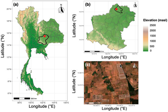
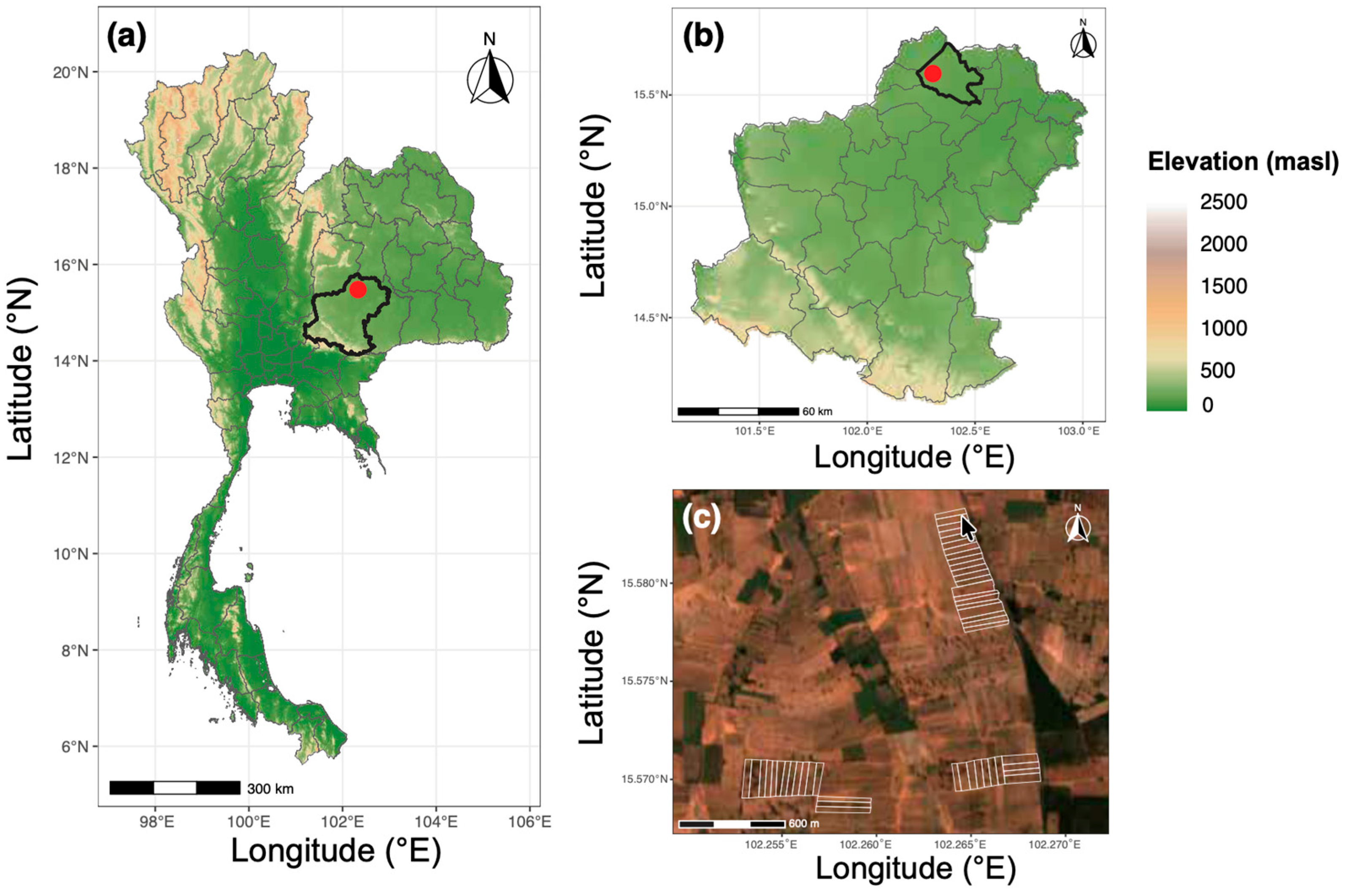
The study site was in Nong Bua Sa-Art Sub-district, Bua Yai District, Nakhon Ratchasima Province. The center of the study site was located at 102.262° N and 15.575° E. The study site included 47 cassava plots with a total area of approximately 0.71 hectare (Figure 1). However, about half of these plots had large trees growing in them (N = 28 out of 47 plots). The study was performed in the 2021/2022 late rainy season. Cassava farmers planted cassava in their plots during slightly different time periods. In our case, most plots began cultivation in December 2021 and completed the season by January 2022. Various cassava varieties were planted in the same plot, primarily Kasetsart 50, Rayong 72, and Huaybong 60. The soil texture is sandy loam with poor water retention. The soil pH ranges from strongly acidic to moderately acidic with low fertility (pH 5.5–7.0). Some areas of the cassava plots are a slope with approximately 2–5% gradient, causing topsoil loss due to rainwater runoff during the rainy season [20]. The rainy season in Thailand typically spans from May to October, followed by the dry season from November to April. However, in 2022, the La Niña phenomenon brought an earlier, longer rainy reason with above-average rainfall [21,22]. As a results, most cassava farmers harvested their crops prematurely in July 2022, only 7–8 months after planting (MAP), to protect the storage roots from rotting due to the excessive moisture caused by La Niña.
Figure 1.
Study site. (a) Thailand with plot site (red dot) in Nakhon Ratchasima Province (black polygon), (b) Nakhon Ratchasima Province with plot site (red dot) in Bua Yai District (black polygon), (c) Plot site at Nong Bua Sa-Art Sub-district, Bua Yai District, including 47 cassava plots (white polygons). The basemaps of (a,b) were CGIAR-SRTM elevation at a resolution of 1 km. The basemap of (c) was a Sentinel-2 image from 26 January 2022, with RGB color compositing at a resolution of 10 m.
2.2. General Workflow and Ground-LAI Measurement
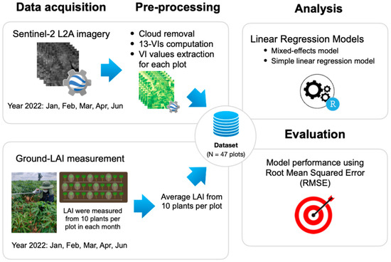
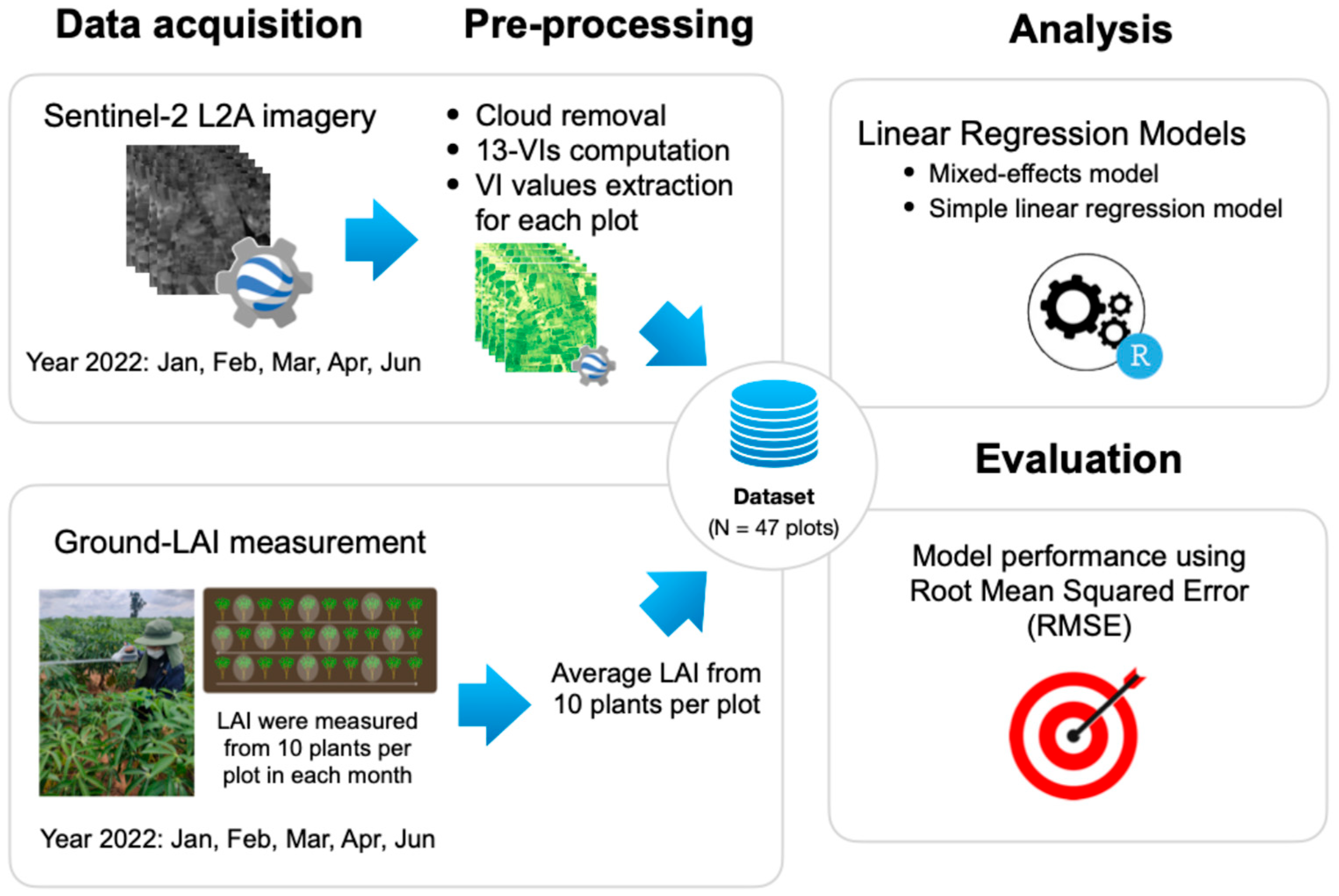
The following sections provide a detailed description of the methodological workflow, outlining the steps taken to acquire and pre-process Sentinel-2 imagery and ground-LAI data, implement the analysis and evaluate the models’ performance in estimating ground-LAI using Sentinel-2 derived vegetation indices (as illustrated in Figure 2).
Figure 2.
Methodological workflow for LAI estimation of cassava using Sentinel-2-derived vegetation indices.
The measurement of ground-level Leaf Area Index (ground-LAI) using an indirect method was conducted from January 2022 (at 2 months after planting, MAP) to June 2022 (at 8 MAP) using a SunScan Canopy Analyzer type SS1 (Delta-T Devices, Cambridge, United Kingdom). The SunScan Canopy Analyzer estimates LAI indirectly from measurements of radiation above and below the canopy, based on a theoretical relationship between leaf area and canopy transmittance [23]. This approach follows the Wood’s (1996) SunScan equations [24], which integrate Campbell’s (1986) analysis [25] of direct solar beam transmission through a canopy with generalized ellipsoidal leaf angle distribution (ELADP) over the whole sky to describe diffuse light transmission. For each plant, solar radiation measurements were taken twice: once above the canopy (full solar radiation) and once under the canopy (shaded by the canopy). These two measurements were then converted to LAI, according to the manufacturer’s protocol [26]. All LAI measurements were conducted under predominantly clear sky conditions.
For plot-level ground-LAI, measurements were collected monthly from all 47 cassava plots in the study. Within each plot, ten cassava plants were randomly selected for sampling, and their measurements were averaged to determine the plot-level LAI. These plot-level values were then averaged to calculate the monthly ground-LAI across the entire study area.
2.3. Preparation of Sentinel-2-Derived Vegetation Indices
2.3.1. Data Acquisition
Acquisition, pre-processing, and VI computation were performed on the Google Earth Engine (GEE) platform [27]. The study employed the data catalog of the Harmonized Sentinel-2 MSI: MultiSpectral Instrument, Level-2A (SR), which was surface reflectance imagery retrieved from Google Earth [28]. The Sentinel-2 imagery provides 13 spectral bands with varying spatial resolution: four bands at 10 m (Blue, Red, Green, and NIR), six bands at 20 m (including Red Edge and SWIR). Images covering the study site at Nong Bua Sa-Art Sub-district, Bua Yai District (bounded by coordinates 102.24965° E, 15.58734° N; 102.24965° E, 15.5596° N; 102.27575° E, 15.5596° N; 102.27575° E, 15.58734° N) were collected for the period between 1 January 2022 and 31 July 2022.
2.3.2. Data Pre-Processing
Preprocessing steps involved multiple operations to enhance data quality. First, the Level-2A data, which had already been atmospherically corrected using a Sen2Cor processor, were further processed to remove cloud contamination [29]. The cloud masking procedure was carried out by using the quality assessment band (QA60) provided with Sentinel-2 products, where bits 10 and 11 indicate the presence of clouds and cirrus clouds, respectively. A bitwise operation was applied to each image to remove cloud- and cirrus-affected pixels. After cloud masking, pixel values were scaled by dividing by 10,000 to convert digital numbers to surface reflectance values. To ensure overall data quality, images with cloud coverage exceeding 20% were completely excluded from the collection. From the preprocessing step, some months yielded only one available image per month. Therefore, we selected the representative image for each month based on the retrieval date closest to the LAI measurement date (Table 1).
Table 1.
List of LAI measurement dates and Sentinel-2 data retrieval dates in each month after planting (MAP) in 2022.
2.3.3. Vegetation Indices (VIs) Computation
This study selected 13 Vegetation Indices (VIs) across different spectral mechanisms to evaluate LAI estimation in cassava using Sentinel-2 data. NDVI, DVI, GNDVI, and GRVI serve as core canopy greenness proxies [15,30,31,32], while SAVI and EVI address soil background interference and NDVI saturation at high LAI values, both of which are common challenges in cassava plots [33,34]. CIG, TCARI, BNDVI, and VIG exploit chlorophyll absorption features that scale with leaf area development [35,36,37,38]. NDWI incorporates canopy water content, which correlates with increasing leaf area [39]. Finally, SeLI and RVI leverage Sentinel-2 red-edge bands, which are particularly sensitive to LAI dynamics in broadleaf tropical crops like cassava [40,41].
The thirteen VIs were implemented within the GEE JavaScript [27] using band arithmetic expressions following the formulas reported in Montero’s study [14], which curated the formulas of novel spectral indices (Table 2). Each index was derived from the corresponding spectral bands of the preprocessed Sentinel-2 images, including visible bands (R, G, and B), Near-infrared (N) band, and two Red Ege bands (RE1 and RE2), and stacked as additional input bands for subsequent analysis. All processed VI layers were subsequently exported as GeoTIFF format at a spatial resolution of 10 m with the WGS84 (EPSG: 4326) coordinate reference system.
Table 2.
Vegetation indices used in this study, including their formulas, Sentinel-2 band assignments, and original references.
For plot-level VIs, satellite imagery was processed to compute monthly VIs. A representative image for each month was selected, and VI values were extracted for each of the 47 cassava plots using zonal statistics with median aggregation that identifies the middle values in the distribution of all pixel values contained within each plot boundary. The analysis was conducted using the ‘terra’ package in R version 4.4.2 [42].
2.4. Statistical Analysis
2.4.1. Regression Analysis Between VIs and Ground–LAI
To evaluate the ability of Sentinel-2-derived-VIs in predicting ground-LAI, we constructed linear mixed-effects models using the ‘lmerTest’ package (version 3.1-3) in R [43]. For each of the thirteen VIs, an individual model was fitted using monthly VI values as fixed-effect predictors and monthly ground-LAI as the response variable. To account for spatial heterogeneity among cassava plots, potentially due to differences in cassava varieties, shading from trees within the plots, or management practices, plot identity was included as a random intercept effect. Temporal dependence was not accessed in this model, because each plot only had one value for each month and the effect of time was examined in separate stage-specific analyses below.
To evaluate the stage-specific performance of each VI during cassava growth, we fitted separate ordinary linear regression models using the ‘stats’ package (version 4.4.2) in R [44], at five distinct stages: 2, 3, 4, 5, and 7 months after planting (MAP). At each growth stage, thirteen models (one per VI) were fitted to determine which indices most accurately predicted ground-LAI at that particular stage of development.
To evaluate the influence of tree presence on model performance, we addressed the imbalanced distribution of plot types (with/without trees) through a rigorous bootstrap validation approach. Given that plots with and without large interspersed trees numbered 28 and 19 respectively, we implemented bootstrapping with 100 iterations to prevent bias toward the more abundant plot type. In each iteration, we randomly resampled data from plots with trees to match the sample size of plots without trees (n = 19) prior to model fitting. This approach generated distributions of RMSE values for each vegetation index, allowing us to calculate mean RMSE, 95% confidence intervals, standard deviations, and coefficients of variation, providing robust estimates of model performance and uncertainty that account for sampling variability.
2.4.2. Evaluation Metrics of Model Performance
Model performance was assessed using multiple evaluation metrics to provide comprehensive assessment of predictive capability. Root Mean Squared Error (RMSE) quantifies the average magnitude of prediction error between observed and predicted LAI values. We selected RMSE due to its interpretability and flexibility: it provides a consistent basis for comparing models fitted with different datasets and is robust for both mixed-effects and linear regression models [45,46]. Lower RMSE values indicate better model performance and higher predictive accuracy. Coefficient of determination (R2) was calculated to assess the proportion of variance in ground-LAI explained by each VI. For linear mixed-effects models, we reported marginal R2 to explain variance by fixed effects of VI only following the method of Nakagawa and Schielzeth [47]. For stage-specific ordinary linear regression models, adjusted R2 was reported to account for model complexity. Statistical significance of the fixed-effect predictor (VI) was evaluated using p-values derived from t-test for fixed effects in mixed-effects models. For stage-specific linear regression models, p-values from the F-test were reported. A significance threshold of α = 0.05 was applied to determine whether the relationship between VI and ground-LAI was statistically significant.
In our study, the datasets used for model fitting differed in sample size; mixed-effects models were built to evaluate the predictive capacity of VIs across all MAPs, whereas stage-specific models were based on subsets of data from individual MAPs. The combination of RMSE, R2, and p-values therefore enabled comprehensive evaluation of model performance, predictive power, and statistical reliability across these varying data structures.
3. Results
3.1. Temporal Patterns of Ground-LAI and Vegetation Indices
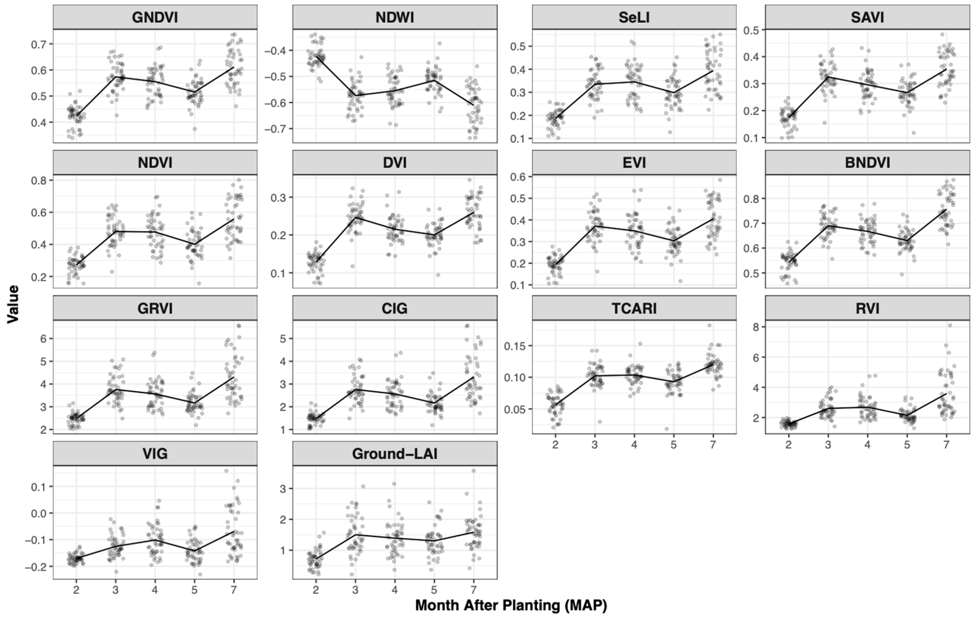
Analysis of temporal patterns of ground-LAI and vegetation indices throughout cassava growth stages (Figure 3 and Figure 4) revealed significant changes corresponding to plant development stages, from emergence, leaf development, and carbohydrate translocation. Ground-LAI increased rapidly from 0.72 ± 0.29 (Mean ± 1 Standard Deviation) at 2 MAP to 1.50 ± 0.60 at 3 MAP, representing the intensive leaf expansion period. Subsequently, ground-LAI decreased slightly at 4 MAP (1.39 ± 0.54) and 5 MAP (1.30 ± 0.46) before increasing again at 7 MAP (1.58 ± 0.55), reflecting the stage of root storage formation.
Figure 3.
Time-series of vegetation indices (VIs) and ground-LAI on cassava plots by Month After Planting (MAP). Points represent values of individual cassava plots. Lines represent average values by MAP.
Figure 4.
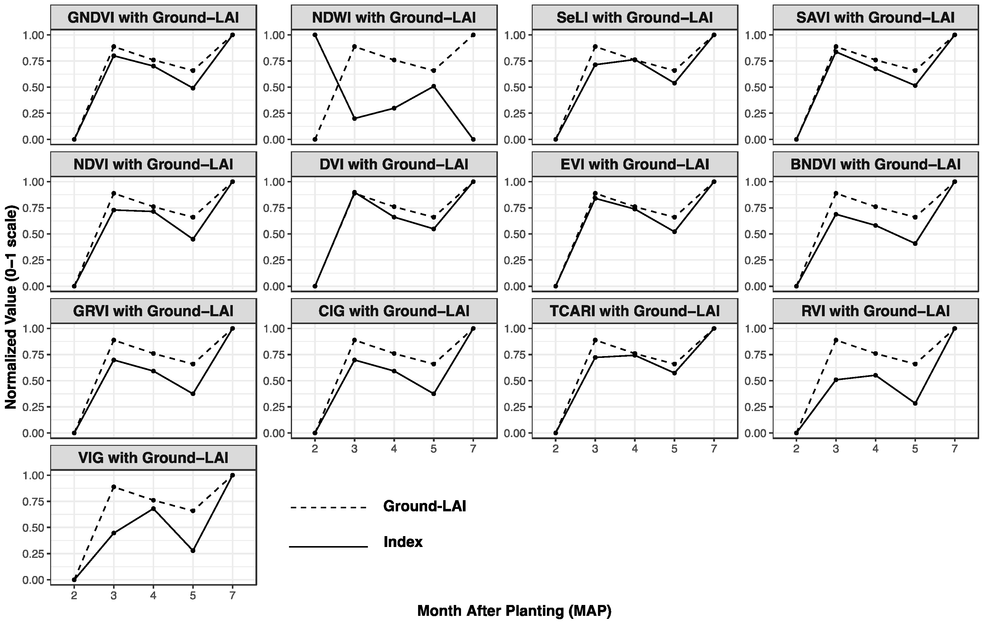
Comparison of vegetation indices (VIs) with ground-LAI for cassava plots by Month After Planting (MAP). Solid lines represent normalized average values of vegetation indices by MAP. Dashed lines represent normalized average values of ground-LAI by MAP.
Most vegetation indices exhibited similar patterns to ground-LAI, particularly GNDVI and NDWI, which showed positive and negative correlations, respectively. GNDVI values increased from 0.42 ± 0.04 at 2 MAP to 0.61 ± 0.07 at 7 MAP, while NDWI showed an opposite trend (−0.42 ± 0.04 to −0.61 ± 0.07). Analysis of normalized values (Figure 4) confirmed that GNDVI had the most consistent pattern with ground-LAI changes.
3.2. Predictive Performance of Vegetation Indices Across All Growth Stages
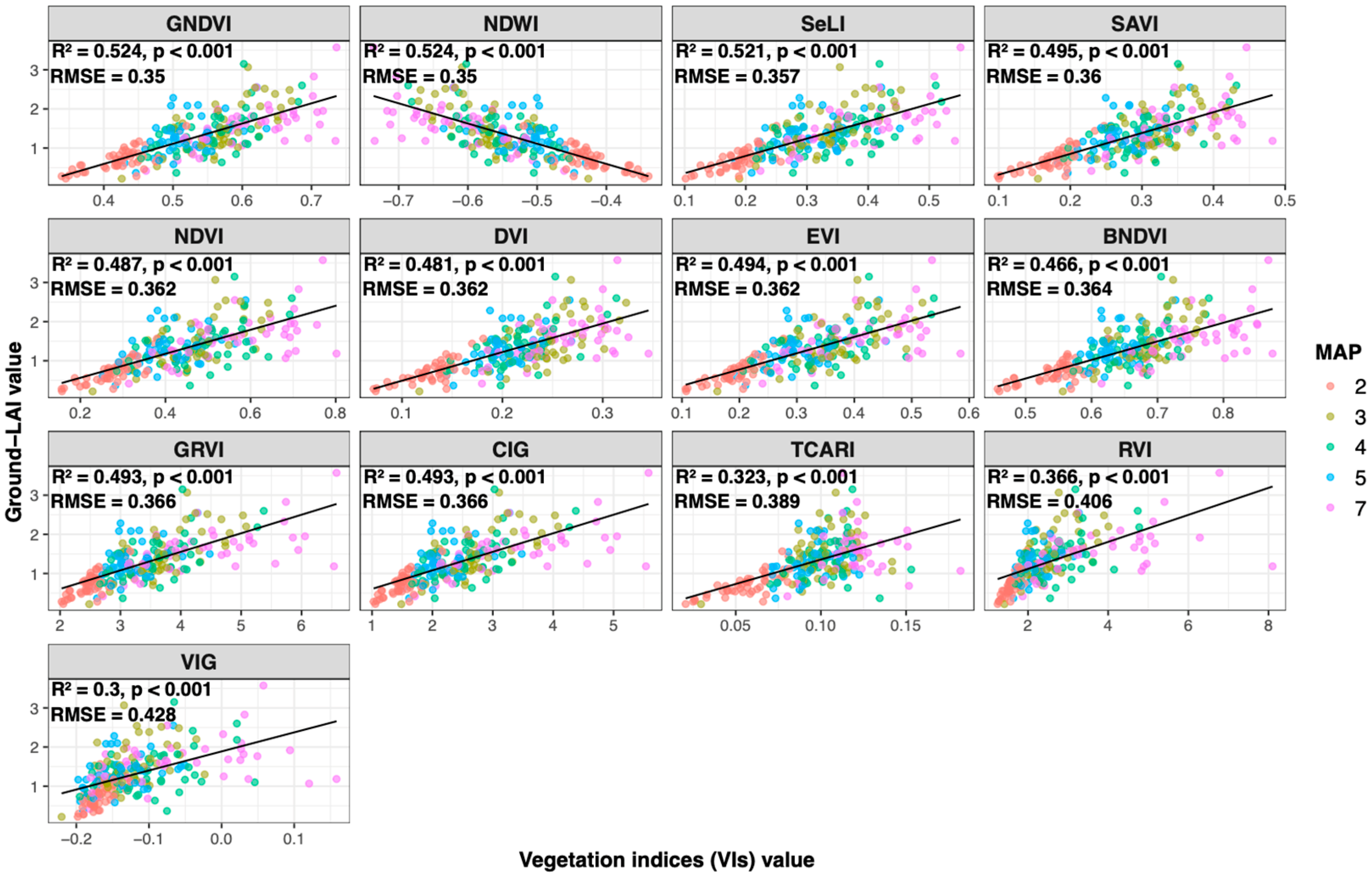
Linear mixed-effects model analysis combining data from all-time points (2–7 MAP) showed that GNDVI and NDWI demonstrated the best performance in predicting ground-LAI with RMSE values of 0.350 (marginal R2 = 0.524, p < 0.001), followed by SeLI (RMSE = 0.357, marginal R2 = 0.521, p < 0.001), SAVI (RMSE = 0.360, marginal R2 = 0.495, p < 0.001), and NDVI (RMSE = 0.362, marginal R2 = 0.487, p < 0.001), while VIG showed the poorest performance (RMSE = 0.428, marginal R2 = 0.300, p < 0.001) (Figure 5; Table S1).
Figure 5.
Vegetation indices (VIs) predictive capability for ground-LAI estimation in all cassava plots (N = 47 plots) across all time points (from 2 MAP to 7 MAP, labelled by different colors of points).
Results indicated that indices incorporating the green band (GNDVI) or related to water content (NDWI) outperformed traditional vegetation indices such as NDVI, possibly due to their higher sensitivity in detecting subtle changes in leaf structure.
3.3. Stage-Specific Performance of Vegetation Indices
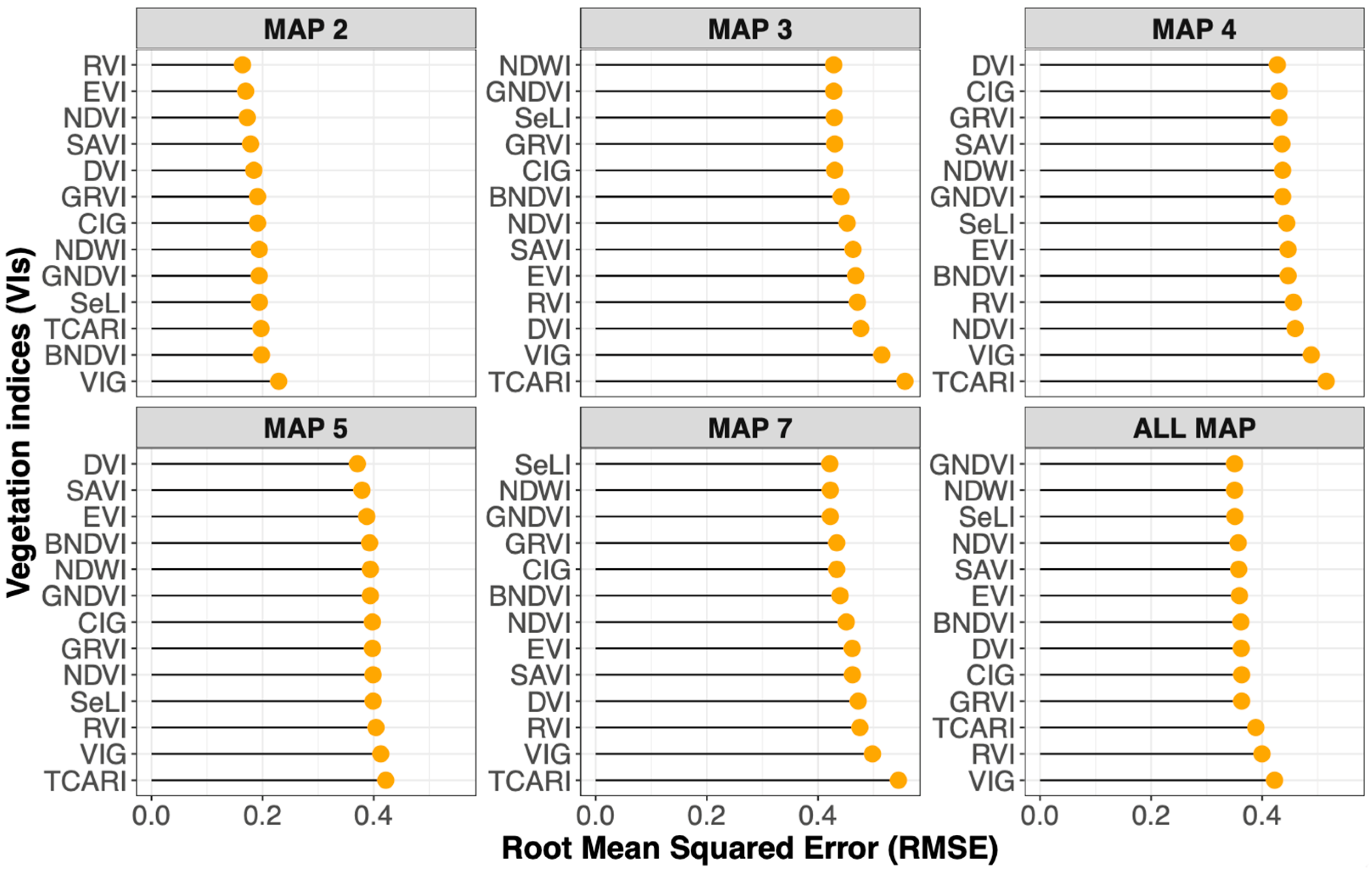
The performance of vegetation indices varied significantly across different growth stages (Figure 6; Tables S2–S6). During the early stage at 2 MAP, RVI demonstrated the best performance (RMSE = 0.164, adjusted R2 = 0.671, p < 0.001) followed by EVI (RMSE = 0.169, adjusted R2 = 0.648, p < 0.001) and NDVI (RMSE = 0.172, adjusted R2 = 0.636, p < 0.001), indicating that when cassava plants are small, indices emphasizing the contrast between NIR and red bands perform better.
Figure 6.
Predictive model performance of vegetation indices (VIs) in predicting ground LAI in all cassava plots (N = 47 plots) by Month After Planting (MAP) and across all time points from 2 MAP to 7 MAP (ALL MAP). Results were ranked by ascending RMSE from linear regression analysis (models by each MAP) and linear mixed-effects model analysis (the model across all MAP).
In the mid-stage from 3 to 5 MAP, GNDVI and NDWI consistently showed high performance, particularly at 3 MAP (RMSE = 0.428, adjusted R2 = 0.473, p < 0.001) with improving trends at 4 to 5 MAP, which corresponds to the period of maximum canopy density. This period represents the most challenging time for LAI estimation due to the complex canopy structure and high biomass density.
At the late stage of 7 MAP, SeLI returned to best performance (RMSE = 0.422, adjusted R2 = 0.393, p < 0.001) along with GNDVI and NDWI, suggesting that the utilization of red edge bands becomes beneficial when cassava plants begin to mature. This shift in optimal indices reflects the changing spectral characteristics of cassava leaves as they age and begin senescence.
3.4. Model Performance Comparison by Plot Types
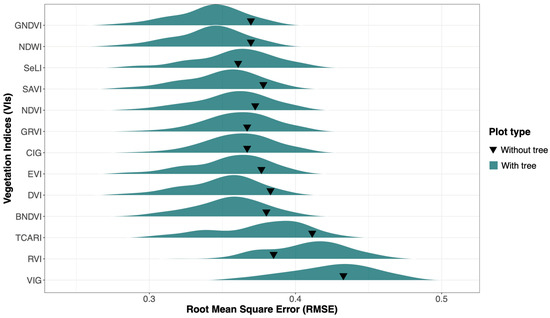
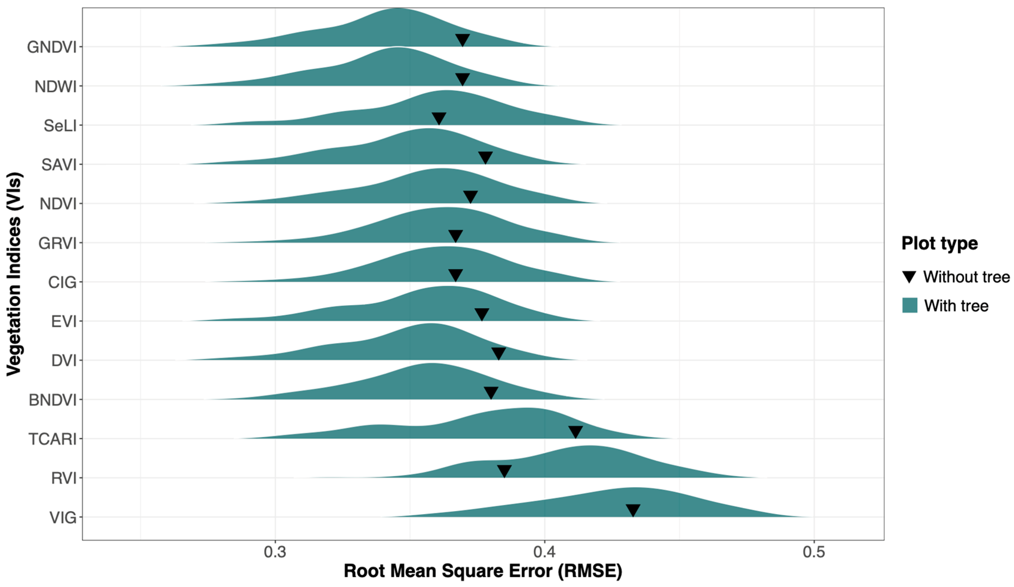
The evaluation of model performance across the plots with trees and without trees revealed that models derived from without-tree plots consistently achieved RMSE values that fell within the 95% confidence interval (95% CI) of the bootstrapping-derived with-tree plot models (Figure 7).
Figure 7.
Comparison of RMSE distributions from VIs models for ground-LAI prediction, between bootstrapping-derived with-tree plots (N = 19, 100 iterations) and without-tree plots (N = 19), ranked by ascending mean RMSE of bootstrapping-derived with-tree plots models.
For models trained on with-tree cassava plots using bootstrap validation (N = 19, 100 iteration; Table 3), the GNDVI and NDWI indices demonstrated that superior performance with the lowest prediction error (mean RMSE = 0.340, 95% CI: 0.286–0.380), followed by the SAVI and DVI indices (both with Mean RMSE = 0.349) ranked as the second-best performers. Conversely, the VIG index exhibited the poorest predictive capability for ground-LAI estimation in with-tree plots (Mean RMSE = 0.425, 95% CI: 0.364–0.573).
Table 3.
Bootstrap validation results for with-tree cassava plots using balanced sampling approach (19 plots randomly sampled from 28, across 100 iterations), ranked by ascending mean RMSE of bootstrapping-derived with tree plots models.
In contrast, models from without-tree plots showed different ranking patterns. The SeLI index achieved the lowest prediction error (RMSE = 0.361), demonstrating its effectiveness in homogeneous cassava environments. This was followed by CIG and GRVI indices (both RMSE = 0.367 and 0.370, respectively), which also ranked among the top three performers for without-tree conditions.
4. Discussion
4.1. Consistency of Ground-LAI and Vegetation Indices
The ground-LAI and VIs generally exhibited similar patterns throughout the growing period, corresponding to cassava growth and development. Cassava growth and development can be categorized into five distinct phases over the 12-month growing period: emergence and sprouting (5–15 days after planting; DAP), initial leaf development and root system formation (15 DAP to 3 months after planting; MAP), leaf development (3–6 MAP), intensive carbohydrate translocation to roots (6–10 MAP), and dormancy (10–12 MAP) [2]. The temporal patterns of ground-LAI and VIs by MAP clearly corresponded to cassava growth stages, showing rapid increases during 2–3 MAP and 5–7 MAP, corresponding to the periods of active leaf development and intensive root storage formation, respectively.
Cassava leaf life typically occurs between 90 and 180 DAP for various genotypes grown under different seasons in Thailand, with leaf life depending on genotype, shade level, and abiotic stresses such as water and temperature [48]. The fallen leaf ratio at 90 DAP was generally smaller than at 180 and 270 DAP for all cassava genotypes and planting dates, indicating a larger portion of leaf discarding in the middle and late growing periods, probably due to leaf senescence and shading effects [48]. This pattern aligns with our observed LAI fluctuations during the mid-growth stages. The older cassava has bigger shrubs that cause less chance for light interception and photosynthesis for lower leaves, ultimately leading to leaf discarding [48].
4.2. Predictive Performance of Vegetation Indices
4.2.1. Overall Performance (All Growth Stages)
Among the thirteen vegetation indices, GNDVI and NDWI demonstrated the best performance in predicting ground LAI across all growth stages, achieving the lowest root mean square error values. These best-performing indices were followed by SeLI, SAVI, and NDVI, respectively. While most temporal patterns of the vegetation indices were similar to ground LAI, their predictive performance differed considerably. Ground LAI estimation based on GNDVI and NDWI was more accurate than those based on other vegetation indices, with the lowest prediction error.
GNDVI demonstrated strong predictive performance for estimating LAI, often outperforming traditional NDVI, especially in dense crop canopies. This superiority is due to the unique properties of the green band. The green band, centered around 560 nm, penetrates the upper canopy layers but is more strongly absorbed by chlorophyll than the red or near infrared bands, making it particularly sensitive to changes in leaf chlorophyll content and new leaf flushing [31,37]. GNDVI, which uses the green and near infrared bands, is more responsive to chlorophyll variations and less prone to saturation in dense canopies compared to NDVI. This allows for better discrimination of canopy health and structure, especially in multilayered or high biomass environments.
A critical advantage of GNDVI is its resistance to saturation at high LAI values. NDVI is prone to saturation when LAI exceeds values between two and three, making it less sensitive to further increases in leaf area in dense crops [49,50,51,52]. In contrast, GNDVI maintains higher sensitivity to LAI across a broader range, especially in dense canopies. Studies in rice and oilseed rape found that GNDVI had higher correlation and lower root mean square error for LAI estimation compared to NDVI [4,37,53]. This characteristic is particularly relevant for cassava monitoring, where LAI values in our study ranged from 0.72 at 2 MAP to 1.58 at 7 MAP.
Both NDVI and GNDVI can be affected by factors such as leaf angle, chlorophyll content, and soil background. However, GNDVI is generally less sensitive to these confounding factors in dense canopies [4,37,54]. NDVI performance is particularly affected by soil background, canopy structure, and non-photosynthetic vegetation, leading to reduced accuracy in complex or mixed vegetation types [52,54,55,56]. Given that many cassava plots in our study contained interspersed trees, with 28 out of 47 plots showing heterogeneous canopy structures, GNDVI’s relative insensitivity to these complications likely contributed to its superior performance. GNDVI can be more sensitive to leaf chlorophyll content and may be influenced by leaf angle and species differences, especially at low LAI [54]. However, our mixed effects modeling approach with plot level random effects helped account for such variations across the three cassava varieties planted, which were Kasetsart 50, Rayong 72, and Huaybong 60.
For Sentinel-2 imagery, NDWI is equivalent to the negative of GNDVI because they use the same bands, including NIR band (B8; 830 nm) and green band (B3; 560 nm). Therefore, they had the same performance, with the lowest RMSE. NDWI and GNDVI from Sentinel 2 both use the green and NIR bands, but their formulas and applications differ [31,39]. Although both indices use the same bands, they invert the numerator, resulting in different sensitivities. NDWI highlights water features and produces positive values for water, while GNDVI highlights green vegetation and yields higher values for healthy, chlorophyll-rich plants. NDWI is optimized for water detection and can also indicate vegetation water content, while GNDVI is tailored for assessing vegetation health and chlorophyll content [54,57,58]. In our cassava study, both indices effectively captured the physiological status of the crop, likely because leaf water content and chlorophyll concentration are closely linked to overall canopy development and LAI.
While different vegetation indices are appropriate for predicting LAI in different crop species, our findings in cassava align with those of studies in rice. Specifically, one study found that GNDVI demonstrated superior performance for LAI estimation across different growth stages in rice with the use of the XGBoost model [4]. Similarly, another study reported that GNDVI showed strong potential for LAI estimation, particularly at early phenological stages in rice [49]. However, studies on LAI estimation across other crops has revealed that the most effective VIs differ considerably among species, such as CI for maize and soybean [9] and NDVI, EVI, and CI for wheat and canola [10]. These diverse outcomes across crop types can be attributed to species-specific differences in phenological patterns, canopy structure and leaf biochemistry, indicating that index selection should be tailored to individual crop species.
4.2.2. Stage-Specific Performance
The performance of vegetation indices in predicting ground-LAI varied significantly across cassava growth stages, with different indices demonstrating lowest prediction errors (RMSE) at different developmental phases. This stage-specific variation reflects the changing spectral characteristics of the canopy and the distinct physiological processes occurring at each growth stage [49,55].
During the initial leaf development phase at 2 MAP, the RVI, EVI, and NDVI demonstrated the highest predictive accuracy (RMSE = 0.164, 0.169, and 0.172, respectively). This superior performance can be attributed to their strong sensitivity to the pronounced NIR-Red contrast when cassava canopies are sparse [49,55,56]. At this stage, healthy cassava leaves reflect strongly in the near-infrared region while absorbing red light due to chlorophyll, resulting in high sensitivity to small variations in LAI [49,55]. These indices maintain linear relationships with LAI at low to moderate levels (LAI < 3–4), making them particularly suitable for early-stage monitoring [49,51,55]. EVI’s incorporation of soil and atmospheric correction factors further enhances accuracy when soil exposure remains substantial during initial leaf development [17].
During the leaf development and canopy establishment phase from 3–5 MAP, GNDVI, NDWI, and DVI consistently outperformed other indices. This period corresponds to maximum canopy density when traditional NDVI typically saturates at LAI > 2–4 due to maximal chlorophyll absorption in the red band and minimal increases in NIR reflectance [50,55,59]. GNDVI’s replacement of the red band with the green band extends the dynamic range and maintains sensitivity at high LAI values when NDVI plateaus [37]. NDWI’s sensitivity to canopy water content and structure further improves LAI estimation in dense vegetation [4]. DVI also demonstrated strong performance during this period, showing high sensitivity to LAI changes and being less prone to saturation effects [60]. The challenging nature of LAI estimation during canopy establishment stems from dense canopies causing overlapping leaves and complex vertical structures that limit light penetration and reduce the sensitivity of most vegetation indices [60].
During the late stage at 7 MAP, when cassava enters initial defoliation and intensive storage root formation, SeLI achieved the best predictive performance (RMSE = 0.422) alongside GNDVI and NDWI. This demonstrates that red-edge bands become particularly beneficial during crop maturation and early senescence. The superior performance of SeLI is driven by the red-edge inflection point’s specific sensitivity to declining chlorophyll content and the onset of leaf yellowing associated with defoliation [8,50,61]. SeLI, utilizing the 705 nm red-edge band, maintains accuracy without saturation effects even at moderate to high LAI values typical during this transition phase [40,50]. Red-edge indices outperform traditional indices during senescence and defoliation due to their enhanced responsiveness to chlorophyll reduction and increased carotenoid-to-chlorophyll ratios, both hallmarks of leaf aging [8,61]. Additionally, the closed canopy structure at this stage minimizes soil background effects, allowing red-edge indices to more accurately reflect canopy physiological status [62].
4.3. Impact of Spatial Heterogeneity on VI Performance
The presence of large trees within cassava plots was common among smallholder farming systems, but it could pose significant challenges for remote sensing-based crop monitoring. Spatial heterogeneity in agricultural landscapes, including variations in crop type, health, soil properties, and management practices, significantly influences spectral reflectance and the accuracy of satellite-based biophysical parameter estimation [63,64,65]. In our study area, 59.6% of plots (28 out of 47) contained large trees growing among cassava plants, creating spatial heterogeneity that potentially affects both cassava growth and the spectral reflectance patterns captured by satellite imagery. This heterogeneity is represented through multiple mechanisms: direct shading effects that reduce photosynthetically active radiation reaching cassava canopies, competition for water and nutrients between established tree root systems and shallow-rooted cassava plants, and the creation of mixed pixels in Sentinel-2 imagery where individual 10 m × 10 m pixels may contain varying proportions of cassava canopy, tree canopy, shadows, and soil background [63,66,67]. At Sentinel-2’s moderate spatial resolution (10 m), such heterogeneity increasingly averages out fine-scale differences, reducing the ability to detect detailed within-plot variability and leading to mixed pixel effects that can compromise the accuracy of vegetation index calculations [63,64,65]. These factors combine to alter both the actual LAI development of cassava and the spectral signatures used to estimate LAI remotely.
The evaluation of the tree effects on model performance revealed differences in the ranking of vegetation index performance between plot types, though importantly, the absolute RMSE values remained comparable. For models trained on with-tree cassava plots using bootstrap validation, the GNDVI and NDWI indices demonstrated superior performance with the lowest prediction error, followed by the SAVI and DVI indices as the second-best performers. The strong performance of GNDVI and NDWI in heterogeneous conditions reflects their ratio-based normalization providing partial illumination invariance, and the green band’s position among the most sensitive spectral regions for crop variability [65,67], while being less affected by shadows than red bands. However, atmospheric scattering and adjacency effects can introduce errors in visible bands within heterogeneous landscapes [68,69], though our use of Sentinel-2 Level-2A atmospherically corrected data helps mitigate these effects. The low coefficient of variation indicates stable performance across different plot combinations.
In contrast, without-tree plots showed different rankings, with SeLI achieving the lowest RMSE, followed by CIG and GRVI. SeLI’s superior performance in homogeneous environments reflects its exploitation of the red-edge region (705 nm and 865 nm), one of the most sensitive spectral regions for crop variability [65,67], with high sensitivity to chlorophyll content and low saturation at high biomass [40]. However, SeLI ranked only eighth in with-tree plots, likely because red-edge bands are more susceptible to shadow contamination and their native 20 m resolution (resampled to 10 m) provides less spatial detail when heterogeneity is present [40,64,70].
Despite the different ranking in model performance, RMSE values from without-tree plots consistently fell within the 95% CI of with-tree bootstrap models for all thirteen indices. For example, GNDVI’s without-tree RMSE (0.370) fell within its with-tree 95% CI (0.286–0.380), and SeLI’s without-tree RMSE (0.361) fell within its with-tree 95% CI (0.294–0.406). This indicated no statistically significant difference in model performance between plot types, despite ranking differences, demonstrating that the evaluated indices were sufficiently robust across varying spatial heterogeneity levels. This robustness was noteworthy given that fragmented parcels with interspersed vegetation are particularly challenging for moderate-resolution satellites [64,70,71].
The range of RMSE values within each plot type (0.085 for with-tree and 0.072 for without-tree, representing 20–25% differences) substantially exceeded typical differences for the same VI across plot types (less than 10%), indicating that VI selection was more critical than plot type for accurate LAI estimation. For heterogeneous landscapes where conditions varied or were unknown, GNDVI or NDWI represented robust choices, performing optimally in with-tree conditions (RMSE = 0.340) while maintaining near-optimal performance in pure cassava plots (RMSE = 0.370). For precision agriculture with well-characterized plots, different indices could be selected in regard to the presence of large trees: GNDVI/NDWI for with-tree plots and SeLI for without-tree plots. While fine spatial resolution imagery (3 m or less) better captures within-plot variability [65,67,72], Sentinel-2’s free availability, frequent revisit, and operational nature make it more practical for regional-scale monitoring.
The low coefficients of variation (0.067–0.082) and overlapping confidence intervals demonstrated that our bootstrap approach successfully handled imbalanced data while capturing generalizable VI-LAI relationships. However, temporal dynamics such as crop growth stages and management practices can alter spatial heterogeneity over time, affecting reflectance patterns [63,66,67]. Our study captured five growth stages (2–7 MAP), but premature harvest due to La Niña prevented observation of the complete 12-month cycle. Future studies should explore additional heterogeneity sources across complete growing seasons to further refine understanding of how environmental complexity influences satellite-based crop parameter estimation.
5. Conclusions
This study systematically evaluated thirteen Sentinel-2-derived vegetation indices for estimating ground-measured LAI in cassava fields, addressing optimal index selection, growth-stage dependent performance, and the small influence of field heterogeneity on model accuracy.
GNDVI and NDWI demonstrated superior performance for ground-LAI estimation across the overall cassava growth trajectory (R2 = 0.524; RMSE = 0.350; p < 0.001), outperforming traditional NDVI (R2 = 0.487; RMSE = 0.362; p < 0.001). Their effectiveness stemmed from enhanced sensitivity to chlorophyll variations, resistance to saturation at higher LAI values, and reduced susceptibility to confounding factors such as soil background and complex canopy structures. Validation against monthly field measurements confirmed their reliability for operational cassava monitoring.
Vegetation index performance varied with cassava’s growth stages. Early stages favored indices emphasizing NIR-Red contrast such as RVI (R2 = 0.671; RMSE = 0.164; p < 0.001), EVI (R2 = 0.648; RMSE = 0.169; p < 0.001), and NDVI (R2 = 0.636; RMSE = 0.172; p < 0.001), which effectively captured sparse canopies. Mid-growth periods at maximum canopy density required saturation-resistant indices, including GNDVI (R2 = 0.473; RMSE = 0.428; p < 0.001), NDWI (R2 = 0.473; RMSE = 0.428; p < 0.001), and DVI (R2 = 0.332; RMSE = 0.427; p < 0.001), to maintain accuracy. Late stages benefited from indices with red-edge bands, such as SeLI (R2 = 0.393; RMSE = 0.422; p < 0.001), which are sensitive to declining chlorophyll during initial defoliation. This phenology-dependent variation necessitates adaptive monitoring strategies aligned with cassava developmental phases.
Spatial heterogeneity from interspersed trees did not significantly compromise model accuracy. Bootstrap validation confirmed that index selection proved more critical than plot type for accurate estimation, with GNDVI and NDWI (mean RMSE = 0.340, 95% CI: 0.286–0.380) maintaining robust performance across both homogeneous and heterogeneous conditions. This validates Sentinel-2 applicability for smallholder farming systems characterized by mixed vegetation landscapes.
Despite the early harvest due to La Niña conditions preventing observation of the complete twelve-month cultivation cycle, this research established a validated methodological framework for satellite-based cassava monitoring. The empirically grounded guidance for vegetation index selection based on growth stage and field conditions provides practical support for developing operational yield forecasting systems and advancing remote sensing applications in tropical root crop production. Future research should extend these approaches across complete growing seasons and diverse agro-ecological zones to further refine predictive capabilities and enhance decision support for sustainable cassava production management.
Supplementary Materials
The following supporting information can be downloaded at: https://www.mdpi.com/article/10.3390/agriengineering8040134/s1, Table S1: Performance metrics of linear mixed-effects models for ground-LAI estimation using Sentinel-2 derived vegetation indices across all growth stages (2–7 MAP). Results were ranked by ascending RMSE; Table S2: Performance metrics of linear models for ground-LAI estimation using Sentinel-2 derived vegetation indices at 2 MAP. Results were ranked by ascending RMSE; Table S3: Performance metrics of linear models for ground-LAI estimation using Sentinel-2 derived vegetation indices at 3 MAP. Results were ranked by ascending RMSE; Table S4: Performance metrics of linear models for ground-LAI estimation using Sentinel-2 derived vegetation indices at 4 MAP. Results were ranked by ascending RMSE; Table S5: Performance metrics of linear models for ground-LAI estimation using Sentinel-2 derived vegetation indices at 5 MAP. Results were ranked by ascending RMSE; Table S6: Performance metrics of linear models for ground-LAI estimation using Sentinel-2 derived vegetation indices at 7 MAP. Results were ranked by ascending RMSE.
Author Contributions
Conceptualization, K.P. and E.K.; methodology, K.P. and E.K.; software, K.P. and E.K.; validation, K.P. and T.J.; formal analysis, K.P. and T.J.; investigation, K.P. and T.J.; writing—original draft preparation, K.P.; writing—review and editing, K.P., P.K. and E.K.; visualization, K.P.; supervision, P.K. and E.K.; project administration, P.K.; funding acquisition, P.K. All authors have read and agreed to the published version of the manuscript.
Funding
This research was partially funded by Digital Economy and Society Development Fund, Ministry of Digital Economy and Society (MDES) of Thailand. K.P.’s graduate scholarship was from Science Achievement Scholarship of Thailand (SAST), through the Office of Higher Education Commission, Ministry of Higher Education, Science Research and Innovation (OPS-MHES).
Data Availability Statement
Data and associated codes in JavaScript and R are available through https://github.com/fonnknp/Sentinel-2-derived-VIs-LAI-on-cassava-plots (accessed on 27 March 2026).
Acknowledgments
We would like to thank the cassava farmers at Nongbua Sa-art, Bua Yai, Nakhon Ratchasima, for allowing us to use their fields and for maintaining the plants throughout the study. We are also grateful to Phongnapha Phanthanong, Sangsuree Thippawan, Napat Jantaraprasit, Patsakorn Tiwutanon, and Pichit Wiroonpan for their assistance in collecting ground-truth data.
Conflicts of Interest
The authors declare no conflicts of interest. The funders had no role in the design of the study; in the collection, analyses, or interpretation of data; in the writing of the manuscript; or in the decision to publish the results.
Abbreviations
The following abbreviations are used in this manuscript:
| LAI | Leaf Area Index |
| VIs | Vegetation Indices |
| RMSE | Root Mean Squared Error |
| CV | Coefficients of Variation |
| 95% CI | 95% of Confidence Interval |
| GEE | Google Earth Engine |
| MAP | Month After Planting |
| R | Red band |
| B | Blue band |
| G | Green band |
| RE1 | Red Edge 1 |
| RE2 | Red Edge 1SW |
| SWIR | Short-wave Infrared |
| NDVI | Normalized Difference Vegetation Index |
| SAVI | Soil-Adjusted Vegetation Index |
| EVI | Enhanced Vegetation Index |
| BNDVI | Blue Normalized Difference Vegetation Index |
| CIG | Chlorophyll Index Green |
| DVI | Difference Vegetation Index |
| GNDVI | Green Normalized Difference Vegetation Index |
| GRVI | Green Ratio Vegetation Index |
| NDWI | Normalized Difference Water Index |
| RVI | Ratio Vegetation Index |
| SeLI | Sentinel-2 LAI Green Index |
| TCARI | Transformed Chlorophyll Absorption in Reflectance Index |
| VIG | Vegetation Index Green |
References
- FAO. FAOSTAT Statistical Database; FAO: Rome, Italy, 2020. [Google Scholar]
- Lebot, V. Tropical Root and Tuber Crops: Cassava, Sweet Potato, Yams and Aroids; CABl: Hong Kong, 2020. [Google Scholar]
- OAE. Cassava: Planting Area, the Number of Smallholders, and the Average Planting Area per Smallholder—The Province Level in 2020; OAE: Bangkok, Thailand, 2020. [Google Scholar]
- Liu, F.; Song, Q.; Zhao, J.; Mao, L.; Bu, H.; Hu, Y.; Zhu, X.G. Canopy occupation volume as an indicator of canopy photosynthetic capacity. New Phytol. 2021, 232, 941–956. [Google Scholar] [CrossRef] [Scilit] [PubMed]
- Hoek van Dijke, A.J.; Mallick, K.; Schlerf, M.; Machwitz, M.; Herold, M.; Teuling, A.J. Examining the link between vegetation leaf area and land–atmosphere exchange of water, energy, and carbon fluxes using FLUXNET data. Biogeosciences 2020, 17, 4443–4457. [Google Scholar] [CrossRef] [Scilit]
- Pipatsitee, P.; Eiumnoh, A.; Praseartkul, P.; Ponganan, N.; Taota, K.; Kongpugdee, S.; Sakulleerungroj, K.; Cha-um, S. Non-Destructive Leaf Area Estimation Model for Overall Growth Performances in Relation to Yield Attributes of Cassava (Manihot esculenta Cranz) under Water Deficit Conditions. Not. Bot. Horti Agrobot. Cluj-Napoca 2019, 47, 580–591. [Google Scholar] [CrossRef] [Scilit]
- Mulla, D.J. Twenty five years of remote sensing in precision agriculture: Key advances and remaining knowledge gaps. Biosyst. Eng. 2013, 114, 358–371. [Google Scholar] [CrossRef] [Scilit]
- Sun, Y.; Qin, Q.; Ren, H.; Zhang, T.; Chen, S. Red-Edge Band Vegetation Indices for Leaf Area Index Estimation From Sentinel-2/MSI Imagery. IEEE Trans. Geosci. Remote Sens. 2020, 58, 826–840. [Google Scholar] [CrossRef] [Scilit]
- Viña, A.; Gitelson, A.A.; Nguy-Robertson, A.L.; Peng, Y. Comparison of different vegetation indices for the remote assessment of green leaf area index of crops. Remote Sens. Environ. 2011, 115, 3468–3478. [Google Scholar] [CrossRef] [Scilit]
- Dong, T.; Liu, J.; Shang, J.; Qian, B.; Ma, B.; Kovacs, J.M.; Walters, D.; Jiao, X.; Geng, X.; Shi, Y. Assessment of red-edge vegetation indices for crop leaf area index estimation. Remote Sens. Environ. 2019, 222, 133–143. [Google Scholar] [CrossRef] [Scilit]
- Serrano Reyes, J.; Jiménez, J.U.; Quirós-McIntire, E.I.; Sanchez-Galan, J.E.; Fábrega, J.R. Comparing Two Methods of Leaf Area Index Estimation for Rice (Oryza sativa L.) Using In-Field Spectroradiometric Measurements and Multispectral Satellite Images. AgriEngineering 2023, 5, 965–981. [Google Scholar] [CrossRef] [Scilit]
- Delegido, J.; Verrelst, J.; Alonso, L.; Moreno, J. Evaluation of Sentinel-2 Red-Edge Bands for Empirical Estimation of Green LAI and Chlorophyll Content. Sensors 2011, 11, 7063–7081. [Google Scholar] [CrossRef] [Scilit]
- Zou, X.; Zhu, S.; Mõttus, M. Estimation of Canopy Structure of Field Crops Using Sentinel-2 Bands with Vegetation Indices and Machine Learning Algorithms. Remote Sens. 2022, 14, 2849. [Google Scholar] [CrossRef] [Scilit]
- Montero, D.; Aybar, C.; Mahecha, M.D.; Wieneke, S. Spectral: Awesome Spectral Indices deployed via the Google Earth Engine JavaScript API. Int. Arch. Photogramm. Remote Sens. Spat. Inf. Sci. 2022, 48, 301–306. [Google Scholar] [CrossRef] [Scilit]
- Rouse, J.W.; Haas, R.H.; Schell, J.A.; Deering, D.W. Monitoring Vegetation Systems in the Great Plains with ERTS; NASA: Washington, DC, USA, 1974. [Google Scholar]
- Pasqualotto, N.; Bolognesi, S.F.; Belfiore, O.R.; Delegido, J.; D’Urso, G.; Moreno, J. Canopy chlorophyll content and LAI estimation from Sentine1-2: Vegetation indices and Sentine1-2 Leve1-2A automatic products comparison. In Proceedings of the 2019 IEEE International Workshop on Metrology for Agriculture and Forestry (MetroAgriFor), Naples, Italy, 24–26 October 2019; pp. 301–306. [Google Scholar]
- Kang, Y.; Özdoğan, M.; Zipper, S.; Román, M.; Walker, J.; Hong, S.; Marshall, M.; Magliulo, V.; Moreno, J.; Alonso, L.; et al. How Universal Is the Relationship between Remotely Sensed Vegetation Indices and Crop Leaf Area Index? A Global Assessment. Remote Sens. 2016, 8, 597. [Google Scholar] [CrossRef] [Scilit]
- Li, W.; Li, D.; Liu, S.; Baret, F.; Ma, Z.; He, C.; Warner, T.A.; Guo, C.; Cheng, T.; Zhu, Y.; et al. RSARE: A physically-based vegetation index for estimating wheat green LAI to mitigate the impact of leaf chlorophyll content and residue-soil background. ISPRS J. Photogramm. Remote Sens. 2023, 200, 138–152. [Google Scholar] [CrossRef] [Scilit]
- Selvaraj, M.G.; Valderrama, M.; Guzman, D.; Valencia, M.; Ruiz, H.; Acharjee, A.; Acharjee, A.; Acharjee, A. Machine learning for high-throughput field phenotyping and image processing provides insight into the association of above and below-ground traits in cassava (Manihot esculenta Crantz). Plant Methods 2020, 16, 87. [Google Scholar] [CrossRef] [Scilit]
- LDD. Soil Series of Bua Yai Distinct, Nakhon Ratchasima Province; Land Development Department (LDD): Bangkok, Thailand, 2018. [Google Scholar]
- CPC. El Niño/Southern Oscillation (ENSO) Diagnostic Discussion-13 January 2022; Climate Prediction Center: College Park, MD, USA, 2022. [Google Scholar]
- TMD. El Niño/La Niña Phenomenon Monitoring; TMD: Bangkok, Thailand, 2022; pp. 1–3. [Google Scholar]
- Oguntunde, P.G.; Olukunle, O.J.; Fasinmirin, J.T.; Abiolu, O.A. Performance of the SunScan canopy analysis system in estimating leaf area index of maize. Agric. Eng. Int. CIGR J. 2012, 14, 1–7. [Google Scholar]
- Wood, J. SunData Software and Canopy Theory; John Wood of Peak Design Ltd.: Derbyshire, UK, 1996. [Google Scholar]
- Campbell, G.S. Extinction coefficients for radiation in plant canopies calculated using an ellipsoidal inclination angle distribution. Agric. For. Meteorol. 1986, 36, 317–321. [Google Scholar] [CrossRef] [Scilit]
- Webb, N.; Nicholl, C.; Wood, J. User Manual for the SunScan Canopy Analysis System Type SS1, Version 3.3 ed.; Delta-T Devices: Cambridge, UK, 2016. [Google Scholar]
- Gorelick, N.; Hancher, M.; Dixon, M.; Ilyushchenko, S.; Thau, D.; Moore, R. Google Earth Engine: Planetary-scale geospatial analysis for everyone. Remote Sens. Environ. 2017, 202, 18–27. [Google Scholar] [CrossRef] [Scilit]
- Google Earth, E. Harmonized Sentinel-2 MSI: MultiSpectral Instrument, Level-2A (SR); Earth Engine Data Catalog; ESA: Paris, France, 2023. [Google Scholar]
- Main-Knorn, M.; Pflug, B.; Louis, J.; Debaecker, V.; Müller-Wilm, U.; Gascon, F. Sen2Cor for Sentinel-2. In Proceedings of the Image and Signal Processing for Remote Sensing XXIII, Warsaw, Poland, 11–14 September 2017; p. 3. [Google Scholar]
- Roujean, J.-L.; Breon, F.-M. Estimating PAR absorbed by vegetation from bidirectional reflectance measurements. Remote Sens. Environ. 1995, 51, 375–384. [Google Scholar] [CrossRef] [Scilit]
- Gitelson, A.A.; Kaufman, Y.J.; Merzlyak, M.N. Use of a green channel in remote sensing of global vegetation from EOS-MODIS. Remote Sens. Environ. 1996, 58, 289–298. [Google Scholar] [CrossRef] [Scilit]
- Sripada, R.P.; Heiniger, R.W.; White, J.G.; Weisz, R. Aerial Color Infrared Photography for Determining Late-Season Nitrogen Requirements in Corn. Agron. J. 2005, 97, 1443–1451. [Google Scholar] [CrossRef] [Scilit]
- Huete, A.R. A soil-adjusted vegetation index (SAVI). Remote Sens. Environ. 1988, 25, 295–309. [Google Scholar] [CrossRef] [Scilit]
- Huete, A.R.; Liu, H.Q.; Batchily, K.; van Leeuwan, W. A comparison of vegetation indices over a global set of TM images for EOS-MODIS. Remote Sens. Environ. 1997, 59, 440–451. [Google Scholar] [CrossRef] [Scilit]
- Gitelson, A.A.; Gritz, Y.; Merzlyak, M.N. Relationships between leaf chlorophyll content and spectral reflectance and algorithms for non-destructive chlorophyll assessment in higher plant leaves. J. Plant Physiol. 2003, 160, 271–282. [Google Scholar] [CrossRef] [Scilit]
- Haboudane, D.; Miller, J.R.; Tremblay, N.; Zarco-Tejada, P.J.; Dextraze, L. Integrated narrow-band vegetation indices for prediction of crop chlorophyll content for application to precision agriculture. Remote Sens. Environ. 2002, 81, 416–426. [Google Scholar] [CrossRef] [Scilit]
- Wang, F.-m.; Huang, J.-f.; Tang, Y.-l.; Wang, X.-z. New Vegetation Index and Its Application in Estimating Leaf Area Index of Rice. Rice Sci. 2007, 14, 195–203. [Google Scholar] [CrossRef] [Scilit]
- Gitelson, A.A.; Kaufman, Y.J.; Stark, R.; Rundquist, D. Novel algorithms for remote estimation of vegetation fraction. Remote Sens. Environ. 2002, 80, 76–87. [Google Scholar] [CrossRef] [Scilit]
- McFeeters, S.K. The use of the Normalized Difference Water Index (NDWI) in the delineation of open water features. Int. J. Remote Sens. 1996, 17, 1425–1432. [Google Scholar] [CrossRef] [Scilit]
- Pasqualotto, N.; Delegido, J.; Van Wittenberghe, S.; Rinaldi, M.; Moreno, J. Multi-Crop Green LAI Estimation with a New Simple Sentinel-2 LAI Index (SeLI). Sensors 2019, 19, 904. [Google Scholar] [CrossRef] [Scilit]
- Birth, G.S.; McVey, G.R. Measuring the Color of Growing Turf with a Reflectance Spectrophotometer. Agron. J. 1968, 60, 640–643. [Google Scholar] [CrossRef] [Scilit]
- Hijmans, R.J. terra: Spatial Data Analysis. 2024. Available online: https://cran.r-project.org/web/packages/terra/index.html (accessed on 9 November 2025).
- Kuznetsova, A.; Brockhoff, P.B.; Christensen, R.H.B. lmerTest Package: Tests in Linear Mixed Effects Models. J. Stat. Softw. 2017, 82, 1–26. [Google Scholar] [CrossRef] [Scilit]
- R Core Team. R: A Language and Environment for Statistical Computing; R Core Team: Vienna, Austria, 2024. [Google Scholar]
- Chai, T.; Draxler, R.R. Root mean square error (RMSE) or mean absolute error (MAE)?—Arguments against avoiding RMSE in the literature. Geosci. Model Dev. 2014, 7, 1247–1250. [Google Scholar] [CrossRef] [Scilit]
- Hodson, T.O. Root-mean-square error (RMSE) or mean absolute error (MAE): When to use them or not. Geosci. Model Dev. 2022, 15, 5481–5487. [Google Scholar] [CrossRef] [Scilit]
- Nakagawa, S.; Schielzeth, H. A general and simple method for obtaining R2 from generalized linear mixed-effects models. Methods Ecol. Evol. 2013, 4, 133–142. [Google Scholar] [CrossRef] [Scilit]
- Phosaengsri, W.; Banterng, P.; Vorasoot, N.; Jogloy, S.; Theerakulpisut, P. Leaf Performances of cassava genotypes in different seasons and its relationship with biomass. Turk. J. Field Crops 2019, 24, 54–64. [Google Scholar] [CrossRef] [Scilit]
- Din, M.; Zheng, W.; Rashid, M.; Wang, S.; Shi, Z. Evaluating Hyperspectral Vegetation Indices for Leaf Area Index Estimation of Oryza sativa L. at Diverse Phenological Stages. Front. Plant Sci. 2017, 8, 820. [Google Scholar] [CrossRef] [Scilit] [PubMed]
- Xie, Q.; Dash, J.; Huang, W.; Peng, D.; Qin, Q.; Mortimer, H.; Casa, R.; Pignatti, S.; Laneve, G.; Pascucci, S.; et al. Vegetation Indices Combining the Red and Red-Edge Spectral Information for Leaf Area Index Retrieval. IEEE J. Sel. Top. Appl. Earth Obs. Remote Sens. 2018, 11, 1482–1493. [Google Scholar] [CrossRef] [Scilit]
- Lykhovyd, P. Sweet Corn Yield Simulation Using Normalized Difference Vegetation Index and Leaf Area Index. J. Ecol. Eng. 2020, 21, 228–236. [Google Scholar] [CrossRef] [Scilit] [PubMed]
- Bajocco, S.; Ginaldi, F.; Savian, F.; Morelli, D.; Scaglione, M.; Fanchini, D.; Raparelli, E.; Bregaglio, S.U.M. On the Use of NDVI to Estimate LAI in Field Crops: Implementing a Conversion Equation Library. Remote Sens. 2022, 14, 3554. [Google Scholar] [CrossRef] [Scilit]
- Han, J.; Song, X.; Zhou, Z.; Chen, Y.; Wei, C.; Liu, W.; Huang, J.; Song, P.; Zhang, D.; Han, B. Estimating leaf area index of winter oilseed rape using high spatial resolution satellite data. In Proceedings of the 2016 Fifth International Conference on Agro-Geoinformatics (Agro-Geoinformatics), Tianjin, China, 18–20 July 2016; pp. 1–5. [Google Scholar]
- Zou, X.; Haikarainen, I.; Haikarainen, I.P.; Mäkelä, P.; Mõttus, M.; Pellikka, P. Effects of Crop Leaf Angle on LAI-Sensitive Narrow-Band Vegetation Indices Derived from Imaging Spectroscopy. Appl. Sci. 2018, 8, 1435. [Google Scholar] [CrossRef] [Scilit]
- Qiao, K.; Zhu, W.; Xie, Z.; Li, P. Estimating the Seasonal Dynamics of the Leaf Area Index Using Piecewise LAI-VI Relationships Based on Phenophases. Remote Sens. 2019, 11, 689. [Google Scholar] [CrossRef] [Scilit]
- Towers, P.C.; Strever, A.; Poblete-Echeverría, C. Comparison of Vegetation Indices for Leaf Area Index Estimation in Vertical Shoot Positioned Vine Canopies with and without Grenbiule Hail-Protection Netting. Remote Sens. 2019, 11, 1073. [Google Scholar] [CrossRef] [Scilit]
- Gao, B.-c. NDWI—A normalized difference water index for remote sensing of vegetation liquid water from space. Remote Sens. Environ. 1996, 58, 257–266. [Google Scholar] [CrossRef] [Scilit]
- Sims, D.A.; Gamon, J.A. Estimation of vegetation water content and photosynthetic tissue area from spectral reflectance: A comparison of indices based on liquid water and chlorophyll absorption features. Remote Sens. Environ. 2003, 84, 526–537. [Google Scholar] [CrossRef] [Scilit]
- Gitelson, A.A. Wide Dynamic Range Vegetation Index for Remote Quantification of Biophysical Characteristics of Vegetation. J. Plant Physiol. 2004, 161, 165–173. [Google Scholar] [CrossRef] [Scilit] [PubMed]
- Jingguo, T.; Shudong, W.; Lifu, Z.; Taixia, W.; Xiaojun, S.; Hailing, J. Evaluating different vegetation index for estimating lai of winter wheat using hyperspectral remote sensing data. In Proceedings of the 2015 7th Workshop on Hyperspectral Image and Signal Processing: Evolution in Remote Sensing (WHISPERS), Tokyo, Japan, 2–5 June 2015; pp. 1–4. [Google Scholar]
- Delegido, J.; Verrelst, J.; Meza, C.M.; Rivera, J.P.; Alonso, L.; Moreno, J. A red-edge spectral index for remote sensing estimation of green LAI over agroecosystems. Eur. J. Agron. 2013, 46, 42–52. [Google Scholar] [CrossRef] [Scilit]
- Xing, N.; Huang, W.; Ye, H.; Dong, Y.; Kong, W.; Ren, Y.; Xie, Q. Remote sensing retrieval of winter wheat leaf area index and canopy chlorophyll density at different growth stages. Big Earth Data 2022, 6, 580–602. [Google Scholar] [CrossRef] [Scilit]
- Zhao, J.; Zhong, Y.; Hu, X.; Wei, L.; Zhang, L. A robust spectral-spatial approach to identifying heterogeneous crops using remote sensing imagery with high spectral and spatial resolutions. Remote Sens. Environ. 2020, 239, 111605. [Google Scholar] [CrossRef] [Scilit]
- Aduvukha, G.R.; Abdel-Rahman, E.M.; Sichangi, A.W.; Makokha, G.O.; Landmann, T.; Mudereri, B.T.; Tonnang, H.E.Z.; Dubois, T. Cropping Pattern Mapping in an Agro-Natural Heterogeneous Landscape Using Sentinel-2 and Sentinel-1 Satellite Datasets. Agriculture 2021, 11, 530. [Google Scholar] [CrossRef] [Scilit]
- Skakun, S.; Kalecinski, N.I.; Brown, M.G.L.; Johnson, D.M.; Vermote, E.F.; Roger, J.-C.; Franch, B. Assessing within-Field Corn and Soybean Yield Variability from WorldView-3, Planet, Sentinel-2, and Landsat 8 Satellite Imagery. Remote Sens. 2021, 13, 872. [Google Scholar] [CrossRef] [Scilit]
- Ding, Y.; Zhao, K.; Zheng, X.; Jiang, T. Temporal dynamics of spatial heterogeneity over cropland quantified by time-series NDVI, near infrared and red reflectance of Landsat 8 OLI imagery. Int. J. Appl. Earth Obs. Geoinf. 2014, 30, 139–145. [Google Scholar] [CrossRef] [Scilit]
- Zhang, D.; Hou, L.; Lv, L.; Qi, H.; Sun, H.; Zhang, X.; Li, S.; Min, J.; Liu, Y.; Tang, Y.; et al. Precision Agriculture: Temporal and Spatial Modeling of Wheat Canopy Spectral Characteristics. Agriculture 2025, 15, 326. [Google Scholar] [CrossRef] [Scilit]
- Houborg, R.; McCabe, M.F. Impacts of dust aerosol and adjacency effects on the accuracy of Landsat 8 and RapidEye surface reflectances. Remote Sens. Environ. 2017, 194, 127–145. [Google Scholar] [CrossRef] [Scilit]
- Choi, W.; Ryu, Y.; Kong, J.; Jeong, S.; Lee, K. Evaluation of spatial and temporal variability in Sentinel-2 surface reflectance on a rice paddy landscape. Agric. For. Meteorol. 2025, 363, 110401. [Google Scholar] [CrossRef] [Scilit]
- Burchard-Levine, V.; Nieto, H.; Riaño, D.; Migliavacca, M.; El-Madany, T.S.; Guzinski, R.; Carrara, A.; Martín, M.P. The effect of pixel heterogeneity for remote sensing based retrievals of evapotranspiration in a semi-arid tree-grass ecosystem. Remote Sens. Environ. 2021, 260, 112440. [Google Scholar] [CrossRef] [Scilit]
- Rossi, C.; McMillan, N.A.; Schweizer, J.M.; Gholizadeh, H.; Groen, M.; Ioannidis, N.; Hauser, L.T. Parcel level temporal variance of remotely sensed spectral reflectance predicts plant diversity. Environ. Res. Lett. 2024, 19, 074023. [Google Scholar] [CrossRef] [Scilit]
- Park, S.; Park, N.-W.; Na, S.-i. An Object-Based Weighting Approach to Spatiotemporal Fusion of High Spatial Resolution Satellite Images for Small-Scale Cropland Monitoring. Agronomy 2022, 12, 2572. [Google Scholar] [CrossRef] [Scilit]

Disclaimer/Publisher’s Note: The statements, opinions and data contained in all publications are solely those of the individual author(s) and contributor(s) and not of MDPI and/or the editor(s). MDPI and/or the editor(s) disclaim responsibility for any injury to people or property resulting from any ideas, methods, instructions or products referred to in the content. |
© 2026 by the authors. Licensee MDPI, Basel, Switzerland. This article is an open access article distributed under the terms and conditions of the Creative Commons Attribution (CC BY) license.