Sensor Layout Optimization and Natural Gas Leakage Source Term Estimation Based on Non-Dominated Sorting Genetic Algorithm

Abstract

For gas leakage monitoring in obstacle environments such as oil and gas stations, the layout of fixed sensors directly affects the validity of monitoring data and the accuracy of subsequent leakage source localization. To achieve effective coverage of high-risk areas with a limited number of sensors and reduce deployment costs, this paper proposes a multi-objective optimization method for sensor layout based on the non-dominated sorting genetic algorithm-II (NSGA-II). Based on multi-scenario computational fluid dynamics simulation data, the peak concentration, hazardous concentration duration, and leakage probability at each monitoring point are extracted as risk characteristic indicators. The NSGA-II analytic hierarchy process is employed to determine the weight of each indicator, and a comprehensive risk classification model for the monitored area is established. This is adopted for solution seeking. Through non-dominated sorting and crowding distance calculation, the Pareto optimal front is searched in the solution space. The optimized layout scheme is applied to the leakage source term estimation based on particle filter, and the performance of different layout schemes is compared and analyzed with the source localization error as the evaluation index. Case studies show that the sensor layout optimized by the non-dominated sorting genetic algorithm achieves effective coverage of high-risk areas. With the same number of sensors, its high-risk area coverage rate outperforms that of the multi-objective particle swarm optimization algorithm (MPSOA). Following the application of the optimized layout, the localization accuracy of leakage source term estimation is significantly improved. Compared with the traditional grid and circular layouts, the source localization error is reduced by approximately 44%. Compared with the layouts optimized by the MPSOA and genetic algorithm (GA), the error is decreased by 30.4% and 33.3%, respectively. The proposed sensor layout optimization method based on the NSGA-II can effectively balance monitoring coverage and economic cost, and significantly improve the localization accuracy of gas leakage sources. This study provides a theoretical basis and technical support for the optimal deployment of fixed gas sensor networks in complex scenarios.

1. Introduction

With the continuous growth of energy demand and the rapid development of the chemical industry, the number of hazardous chemical production and storage facilities such as oil and gas stations and hydrogen refueling stations has increased. Once a gas leakage accident occurs in these places, it is very likely to cause catastrophic consequences such as fire and explosion, posing a serious threat to the safety of people’s lives and property as well as the ecological environment [1,2]. Therefore, the establishment of an efficient and reliable fixed gas sensor network is of great significance for ensuring industrial production safety and improving emergency response capabilities [3]. A reasonable sensor layout can quickly capture concentration signals in the early stage of leakage, providing key data support for subsequent leakage source localization and emergency decision-making [4,5].

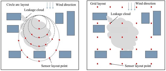
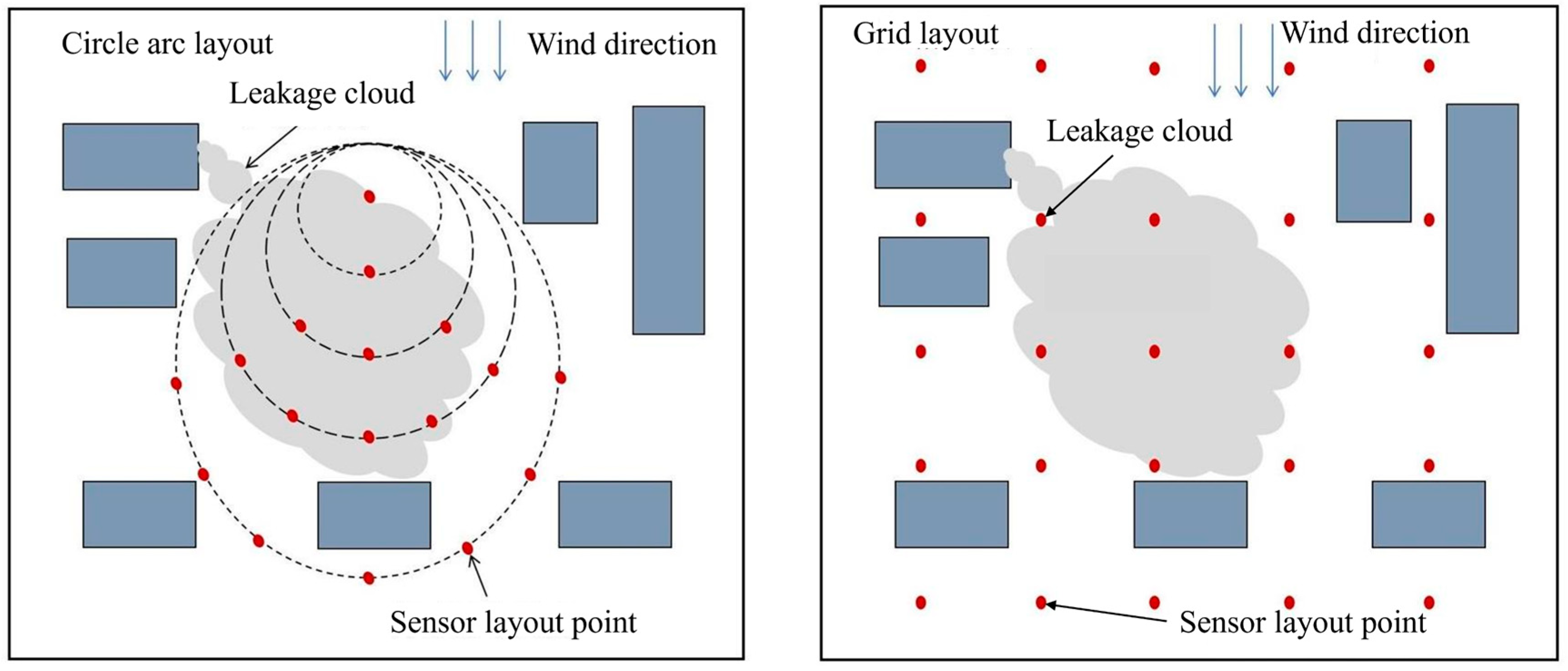
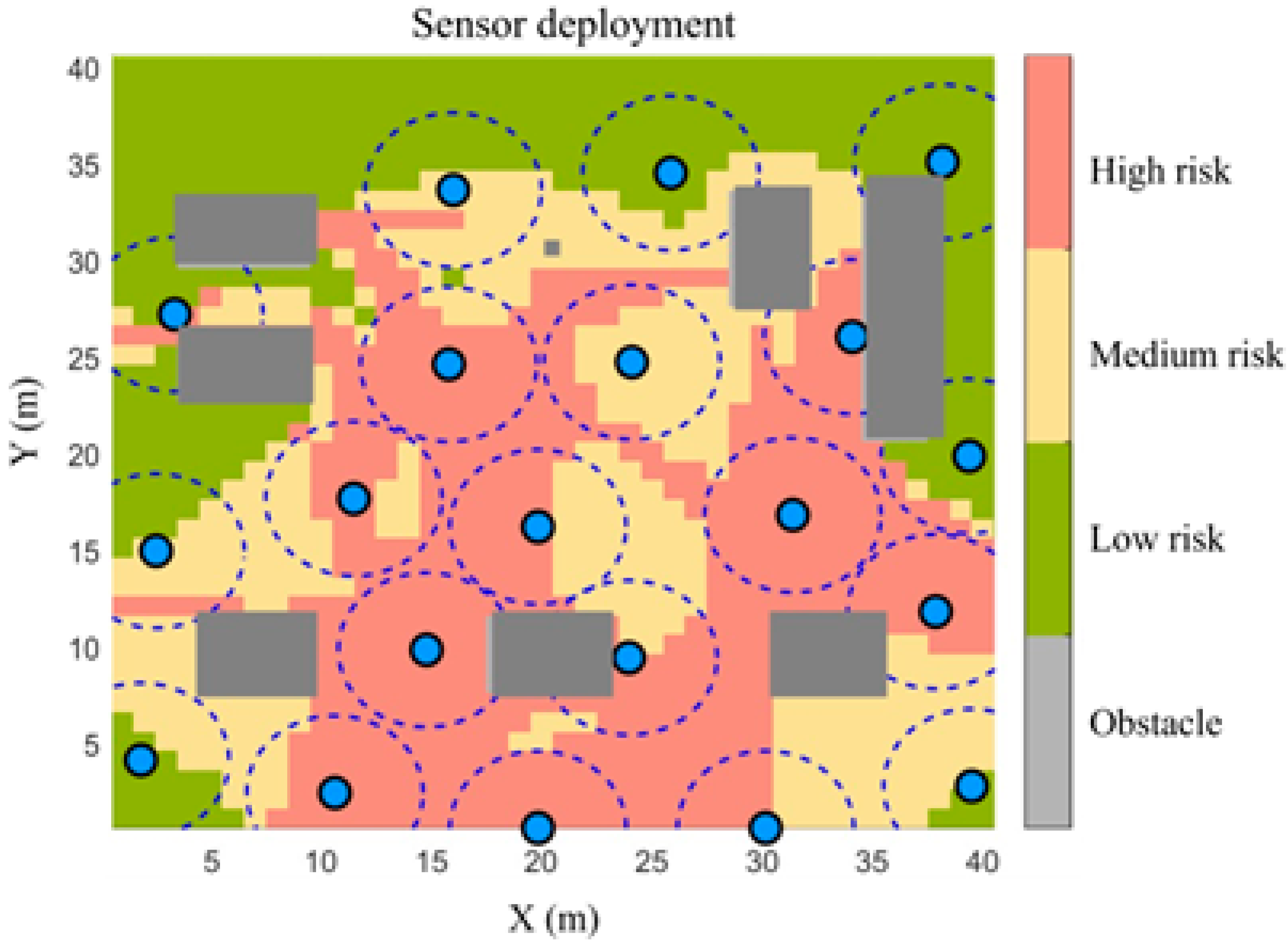
Traditional grid and circular arc layouts are commonly used because of their simple implementation, as illustrated in Figure 1. However, these layouts mainly rely on geometric rules and do not fully consider gas dispersion characteristics, obstacle effects, or spatial risk differences.

Figure 1. Traditional sensor layouts.

In recent years, scholars at home and abroad have carried out extensive research on the optimization of gas sensor layout, forming a diverse methodological system. Benavides et al. [6] proposed a stochastic algorithm that guides sensor placement by minimizing risk values while accounting for sensor errors, and performs numerical optimization using diffusion simulations. Compared with other methods, this approach improves sensor performance. Cen et al. [7] proposed a quantitative filtering method to select representative leakage scenarios from all leakage scenarios, and presented a stochastic mixed-integer linear programming model based on leakage risk to guide sensor layout, reducing the leakage risk under all possible conditions to a certain extent. Following the research idea of optimizing sensor layout based on risk control, other scholars have further expanded the application scenarios and optimization objectives. Legg et al. [8,9] formulated the sensor placement problem as an optimization problem. In the FLACS environment, they guided the sensor layout by minimizing the detection time while ensuring sensor coverage, and proposed a stochastic programming method to solve the optimization problem. Zhou et al. [10] proposed a stochastic programming method to optimize the placement of gas detectors. They transformed the optimal sensor layout problem into minimizing gas leakage risk, and then adopted the particle swarm optimization algorithm to solve the optimization problem, thus improving the performance of the gas detection system. In addition to stochastic programming, integer linear programming and the set covering problem have also become important tools for sensor layout optimization, with more emphasis on multi-objective balance. Oleynik et al. [11] employed the set covering problem to design the sensor array layout, taking the minimization of sensor quantity, sensor cost, and leakage probability as constraints for sensor placement. Rad et al. [12] extended integer linear programming to address the two optimization objectives of maximizing sensor coverage and minimizing detection time, and introduced a multi-level voting mechanism to ensure the effectiveness of sensor placement.

Information theory has also been introduced into sensor layout design, focusing on reducing information redundancy and improving information acquisition efficiency. Khorshidi et al. [13] proposed a sensor placement strategy based on a hybrid information entropy optimization framework to identify leaks in water distribution networks. By maximizing the value of information and minimizing the mutual information entropy, the strategy ensures that sensors capture more information while minimizing the number of sensors used. Terman et al. [14] adopted a similar approach: they minimized the mutual information between sensor pairs to avoid redundant information, while maximizing the total information to ensure that the sensor network obtained the maximum information. This allows more information to be captured with the same number of sensors. Kwak et al. [15] proposed a mixed-integer linear programming model that minimizes risk by reflecting regional characteristics, and compared the exposed area and residual risk score. The method is suitable for cities with uneven distribution of characteristics. On the other hand, the correlation between sensor layout and source term estimation has also attracted the attention of researchers, who have explored the optimal layout from the perspective of improving estimation accuracy. Ma et al. [16] proposed an active firefly algorithm for source term estimation in gas dispersion and investigated the influence of sensor placement on the performance of the active firefly algorithm. Lang et al. [17] captured data using uniformly arranged sensors and combined sensor data with an atmospheric dispersion model via cluster analysis and proposed a multi-sensor data-driven source term estimation model, which improved computational efficiency compared with traditional direct methods and neural network methods. Shui et al. [18]. constructed a comprehensive leakage scenario set using Latin hypercube sampling over leak location, orifice size, direction, and wind field, and then optimized detector layouts under an explicit scenario-coverage constraint based on time-varying concentration outputs at monitoring points from CFD. Liu et al. [19] used MILP to optimize sensor placement in a small hydrogen cylinder compartment with 12 candidate positions, balancing coverage and detection time. Due to entropy being an important concept in stochastic theory, it can objectively measure the information gain brought about by sensor deployment. Its physical significance is closely related to source term evaluation and is more suitable for the quantification of methane emissions. Detailed comparisons are summarized in Table 1.

Table 1. Comparison of existing gas sensor deployment mechanisms.

Deployment Mechanisms	Advantages	Limitations
Traditional grid layout	Straightforward design and deployment; convenient for routine maintenance	Neglects gas diffusion laws and poor data collection efficiency
Stochastic programming	Capable of coping with leakage uncertainties; applicable to risk-oriented decision analysis	Demands abundant representative leakage working conditions
Information theory	Cuts redundant sensor readings and boosts the efficiency of information capturing	Information obtained cannot fully reflect safety risks or source positioning precision
Risk-based layout	Closely correlated with on-site safety demands	Estimation precision relies heavily on risk modeling and assigned risk weights

Traditional grid-based and circular deployment methods have been widely used in gas sensor networks. However, uniform layouts are usually adopted, and spatial risk differences are not considered. Information-theory-based methods have also been applied, but redundancy reduction is mainly focused on, while direct risk interpretation is limited. Stochastic and integer programming methods have been introduced, but strong dependence on scenario settings and simplification of dispersion effects are still observed. In addition, PSO- and GA-based methods have been used for optimization; however, premature convergence and weight sensitivity in multi-objective transformation are often reported [20,21].

Therefore, risk-weighted and obstacle-aware characteristics are not fully incorporated in existing studies. Meanwhile, the trade-off between coverage performance, deployment cost, and source estimation accuracy is not sufficiently balanced. In this study, a NSGA-II-based multi-objective optimization framework is proposed. Risk-weighted coverage and deployment cost are simultaneously considered, and Pareto optimal solutions are generated to improve sensor layout quality in obstacle-present gas leakage environments.

Based on the above analysis, this paper proposes a fixed gas sensor layout method that integrates risk classification and multi-objective optimization. Firstly, a comprehensive risk classification model is constructed based on computational fluid dynamics simulation data. Secondly, with the objectives of maximizing risk-weighted coverage and minimizing deployment cost, the NSGA-II is adopted to obtain the optimal layout scheme. Finally, the effectiveness of the proposed method is verified by comparing the localization errors of leakage sources, so as to provide a theoretical basis and technical support for the optimal deployment of gas sensor networks in complex scenarios.

2. Methodology

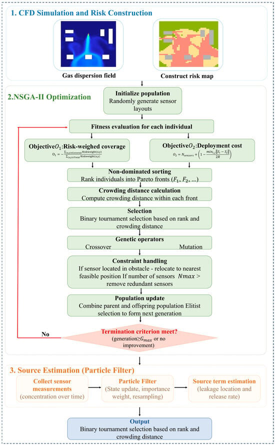
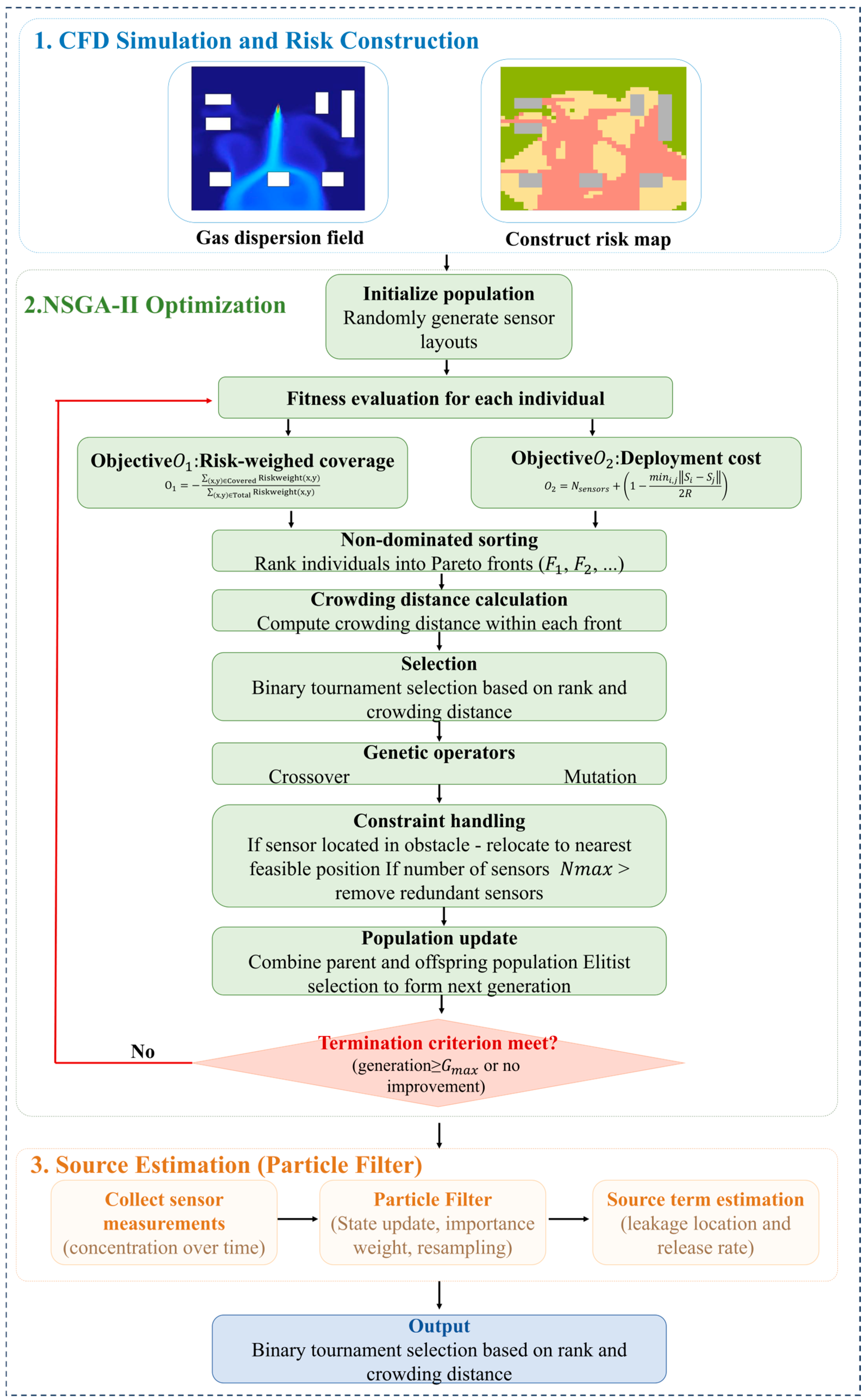
The sensor layout optimization and gas leakage source term estimation method proposed in this study is illustrated in Figure 2. First, computational fluid dynamics is employed to construct gas diffusion contours in obstacle-present scenarios. A comprehensive risk index is then calculated using parameters such as peak concentration and leakage probability, based on which risk classification is performed. NSGA-II is adopted for multi-objective optimization of sensor layout, and the optimal layout scheme is extracted from the Pareto optimal front. Then, particle filtering based on Bayesian theory is applied for gas leakage source term estimation. The main steps of the proposed method are shown in Figure 2. Each step and its underlying principle will be elaborated in detail in the subsequent sections.

Figure 2. Steps of the sensor layout optimization and source estimation.

2.1. Non-Dominated Sorting Genetic Algorithm-II

Gas sensor layout optimization is a typical multi-objective optimization problem in the field of wireless sensor network topology planning. Studying gas sensor layout is essential to investigate the problem of maximizing the coverage of the monitoring network composed of fixed sensors and minimizing the cost consumption. To quantify the theoretical conditions of this problem, certain assumptions are required: sensor nodes exhibit isomorphic characteristics, with fixed sensing radius and communication radius; there is no functional coupling between nodes in the topology, and the working state of each node satisfies the independence condition; and the system operates in an idealized two-dimensional plane, ignoring spatial heterogeneity such as terrain undulations. Based on the above assumptions, the sensor layout optimization problem can be modeled as follows: within a given area $A\in R^2$, the spatial coordinate configuration is performed for the sensor set $S=\{s_1 ,s_2 ,\dots ,s_n\}$. The coordinate configuration should simultaneously satisfy the optimal solution set of the objective functions, namely, maximizing the risk coverage $\mathit{max}\left\{U_{i=1}^{n}C(s_i)\right\}$ and minimizing the deployment cost $\mathit{min}\left\{{\sum }_{i=1}^{n}F(s_i)\right\}$, where $C(s_i)$ denotes the circular monitoring range of the sensor and $F\left(s_i\right)$ represents the cost function.

In this study, fixed methane gas concentration sensors are considered for natural gas leakage monitoring. Since methane is the main component of natural gas, methane concentration is used as the monitoring variable. The sensors are assumed to be homogeneous, and each sensor has the same sensing radius, detection threshold, response characteristics, and measurement accuracy. In the numerical case, the sensing radius of each sensor is set to 4 m. The detection threshold of gas sensors is set to $5\times {10}^{-4} \mathrm{k}\mathrm{g}/{\mathrm{m}}^3$, with a detection rate of 70%.

Sensor layout optimization, as a typical multi-objective optimization problem, is solved in this section using the NSGA-II. The algorithm achieves a dynamic balance between objective functions in the solution space by constructing a multi-objective Pareto optimal set. Its core framework consists of the following three parts:

Hierarchical sorting based on the Pareto dominance relation: non-dominated sorting is performed on individuals in the population by establishing the Pareto dominance criterion to construct a hierarchical optimization structure. For any two solution vectors $A$ and $B$, solution $A$ dominates solution $B$ if and only if $f_i(A)\le f_i(B)\left(i=\mathrm{1,2},\dots m\right)$ and there exists at least one objective j such that $f_j(A)\le f_j(B)$.

Non-dominated individuals are recursively selected to form front ranks, which constitute the convergence guidance criterion of the algorithm. Self-adaptive genetic operation system: using the binary tournament strategy, fitness evaluation is carried out based on the dual indicators of individual rank and crowding distance, so as to ensure the directional transmission of superior genes. The crossover probability is controlled based on the distribution index to achieve continuous recombination of the characteristic parameters of the parent individuals. Mutation probability is introduced to maintain population diversity and prevent the algorithm from falling into local optima. Elite Preservation Strategy and Crowding Distance Sorting: By constructing a combined population consisting of parent and offspring individuals, an elite preservation strategy is employed to select non-dominated solutions. The crowding distance metric is used to quantify the distribution density of the solution set, and individuals in higher front ranks and sparser regions are retained preferentially, which effectively balances the convergence speed and the distribution uniformity of the solution set.

The core of multi-objective optimization lies in constructing a reasonable objective function. In sensor layout optimization, the spatial distribution parameters of sensors (including quantity configuration and position selection) are systematically adjusted to seek the Pareto optimal solution between maximizing risk coverage and minimizing deployment cost. Herein, risk coverage refers to the monitoring capability of the sensor network for high-risk areas, which should ensure that high-risk locations have priority for coverage. Deployment cost is mainly reflected in minimizing the number of sensors, that is, achieving optimal resource allocation on the premise of satisfying monitoring requirements. Therefore, the objective functions are designed as follows:

Equation (1) defines the risk-weighted coverage objective of the deployed sensor network:

$$O_1=-{\displaystyle \frac{{\sum }_{\left(x,y\right)\in Covered}Riskweight(x,y)}{{\sum }_{\left(x,y\right)\in Total}Riskweight(x,y)}}$$

(1)

In this formulation, the numerator represents the total risk weight of all grid cells that are successfully covered by at least one sensor. Each grid cell is assigned a risk weight $Riskweight(x,y)$, which is obtained from CFD-based simulation results, including peak gas concentration, hazardous exposure duration, and leakage probability.

The denominator represents the total risk weight of the entire monitoring region, which is used as a normalization factor to ensure comparability across different scenarios.

The ratio, therefore, represents the fraction of total risk that is successfully monitored by the sensor network. A higher value indicates better coverage of high-risk regions.

A negative sign is introduced because the NSGA-II framework is formulated as a minimization problem. Therefore, maximizing risk coverage is equivalently converted into minimizing the uncovered risk ratio.

Equation (2) defines the deployment cost function of the sensor network:

$$O_2={\displaystyle \frac{N_{sensors}}{N_{max}}}+\left(1-{\displaystyle \frac{{\mathit{min}}_{i,j}‖S_i-S_j‖}{2R}}\right)$$

(2)

In this expression, the first term $N_{sensors}$ represents the total number of deployed sensors, which directly reflects installation and maintenance cost, and $N_{max}$ is the maximum allowable number of sensors. A smaller number of sensors indicates lower deployment cost.

The second term is introduced as a spacing penalty term, which is used to avoid excessive clustering of sensors.

$S_i,S_j$ represent the spatial positions of sensor $i$ and sensor $j$, respectively;

${\mathit{min}}_{i,j}‖S_i-S_j‖$ represents the minimum distance between any pair of sensors in the deployment scheme;

$R$ is the sensing radius of a single sensor.

The term $\left(1−{\displaystyle \frac{{\mathrm{m}\mathrm{i}\mathrm{n}}_{i,j}\parallel S_i-S_j\parallel }{2R}}\right)$ penalizes cases where sensors are placed too close to each other. When sensors are densely clustered, the minimum distance becomes small, leading to a larger penalty value. Conversely, when sensors are well separated, the penalty approaches zero.

The normalization by $2R$ ensures that the spacing constraint is consistent with the physical sensing range, preventing redundant overlap between adjacent sensors.

According to the established objective functions, the flow of the sensor layout optimization algorithm is shown in Algorithm 1.

Algorithm 1 NSGA-II Based Sensor Layout Optimization

Input: ·Risk map $R(x, y)$ ·Maximum number of sensors $Nmax$ ·Population size $P$ ·Maximum generations $Gmax$ Output: ·Optimal sensor layout $X^{*}$ (selected from Pareto front) 1: // Initialization 2: t = 0; 3: Generate initial population $X(t) = \{X1, X2,..., Xp];$ 4: Evaluate objectives $O_1$ and $O_2$ for all individuals; 5: // Evolution process 6: while $(t < G_{max})$ do 7: Perform non-dominated sorting and obtain fronts $F1, F2 ,...;$ 8: Calculate crowding distance for individuals in each front; 9: Select parents by binary tournament selection; 10: Apply crossover to generate offspring population $Q(t)$; 11: Apply mutation to $Q(t)$; 12: Handle constraints (obstacle avoidance and $N_{max}$); 13: Evaluate objectives $O_1$ and $O_2$ for all offspring; 14: Combine $R(t)= X(t)\mathrm{U}Q(t)$; 15: Perform non-dominated sorting on $R(t)$; 16: Fill next population $X(t + 1)$ using elitist strategy basedon rank and crowding distance; 17: $t=t+1$; 18: end while 19: // Output 20: Obtain Pareto front $F_1$ from the final population; 21: Select best compromise solution $X^{*}$from $F_1$; 22: return $X^{*}$; Symbols Explanation: $R\left(\mathrm{x},\mathrm{y}\right):$ Risk weight of grid cell $(x, y)$ $O_1$: Risk-weighted coverage objective $(\mathrm{E}\mathrm{q}\mathrm{u}\mathrm{a}\mathrm{t}\mathrm{i}\mathrm{o}\mathrm{n}(1))$ $O_2$: Deployment cost objective $(\mathrm{E}\mathrm{q}\mathrm{u}\mathrm{a}\mathrm{t}\mathrm{i}\mathrm{o}\mathrm{n}(2))$ $N_{max}$: Maximum allowable number of sensors $P$: Population size $G_{max}$: Maximum number of generations $X\left(t\right)$: Population at generation $t$ $Q(t)$: Offspring population at generation $t$ $F_i$: $i-th$ Pareto front

2.2. Particle Filtering

Particle filtering, as a classic method in data assimilation, is widely used in the source term estimation of atmospheric pollutants and the parameter estimation of radiation sources. In the leakage source localization method based on Bayesian theory, the prior information of the natural gas leakage source is converted into posterior information combined with the concentration data from gas sensors [22,23]. The theoretical basis of Bayesian theory is shown as follows:

$$P\left(m|n\right)={\displaystyle \frac{P(n|m)p(m)}{p(n)}}\propto P(n|m)p(m)$$

(3)

where $m(x,y)$ represents the parameters of the natural gas leakage source, including its position coordinates. $N(n_1 ,n_2 ,\dots ,n_k )$ denotes the concentration data measured by gas sensors.

$P(m)$ is the prior distribution of the natural gas leakage source term parameters calculated from prior information. In complex environments, the prior information of natural gas leakage sources is difficult to obtain, and a uniform distribution is generally adopted. $P(n)$ is the posterior distribution of the natural gas leakage source parameters. $P(n\mid m)$ refers to the likelihood probability of the gas sensor concentration given the natural gas leakage source parameters, also known as the likelihood function. $P(m\mid n)$ represents the probability distribution of the natural gas leakage source term parameters.

The selection of the likelihood probability determines the stability and accuracy of the inversion model, which is jointly affected by the systematic error ${\epsilon }_1$ of natural gas sensors and the error ${\epsilon }_2$ of the gas dispersion model. In general, these two errors approximately follow normal distributions, namely ${\epsilon }_1~N(0,{{\sigma }_1}^2)$ and ${\epsilon }^2~N\left(0,{{\sigma }_2}^2\right).$

$$P(n\mid m)={\displaystyle {\prod }_{i=1}^k}(n_i\mid m)\propto \mathit{exp}\{-{\displaystyle \frac{[f(m)-n_i{]}^2}{2({\sigma }_{1,i}^2+{\sigma }_{2,i}^2)}}\}$$

(4)

where $n_i$ denotes the actual measured value of the gas sensor, and $f(m)$ represents the output value of the natural gas dispersion model.

The specific steps of particle filtering are as follows:

(1) A uniform distribution is chosen as the prior distribution of the natural gas leakage source term. The particle swarm $[Xi(x,y\left)\right]$ is initialized, and the initial weight of each particle is assigned as $w=1/k$.

(2) Update the particle states at the j step. For the particle set $i=\mathrm{1,2},\dots ,k$, the importance weight of each particle is calculated according to the likelihood function, and the weights are normalized.

$$w_i(j)={\displaystyle \frac{w[X_i(j)]}{{\sum }_{i=1}^{k}w[X_i(j)]}}$$

(5)

(3) To alleviate the problem of particle degeneracy, the effective sample size Neff is defined. Resampling is required when $Neff$ is smaller than a preset threshold. Such resampling duplicates high-weight particles multiple times, resulting in the loss of particle diversity.

$$Neff={\displaystyle \frac{1}{{\sum }_{i=1}^N[w_i(j){]}^2}}$$

(6)

(4) After several iterations, the particles converge to the high-likelihood region of the leakage source parameters. The estimated parameters of the natural gas leakage source can then be obtained by calculating the mean of the particles.

3. Result and Discussion

3.1. Simulation Case Results

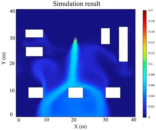
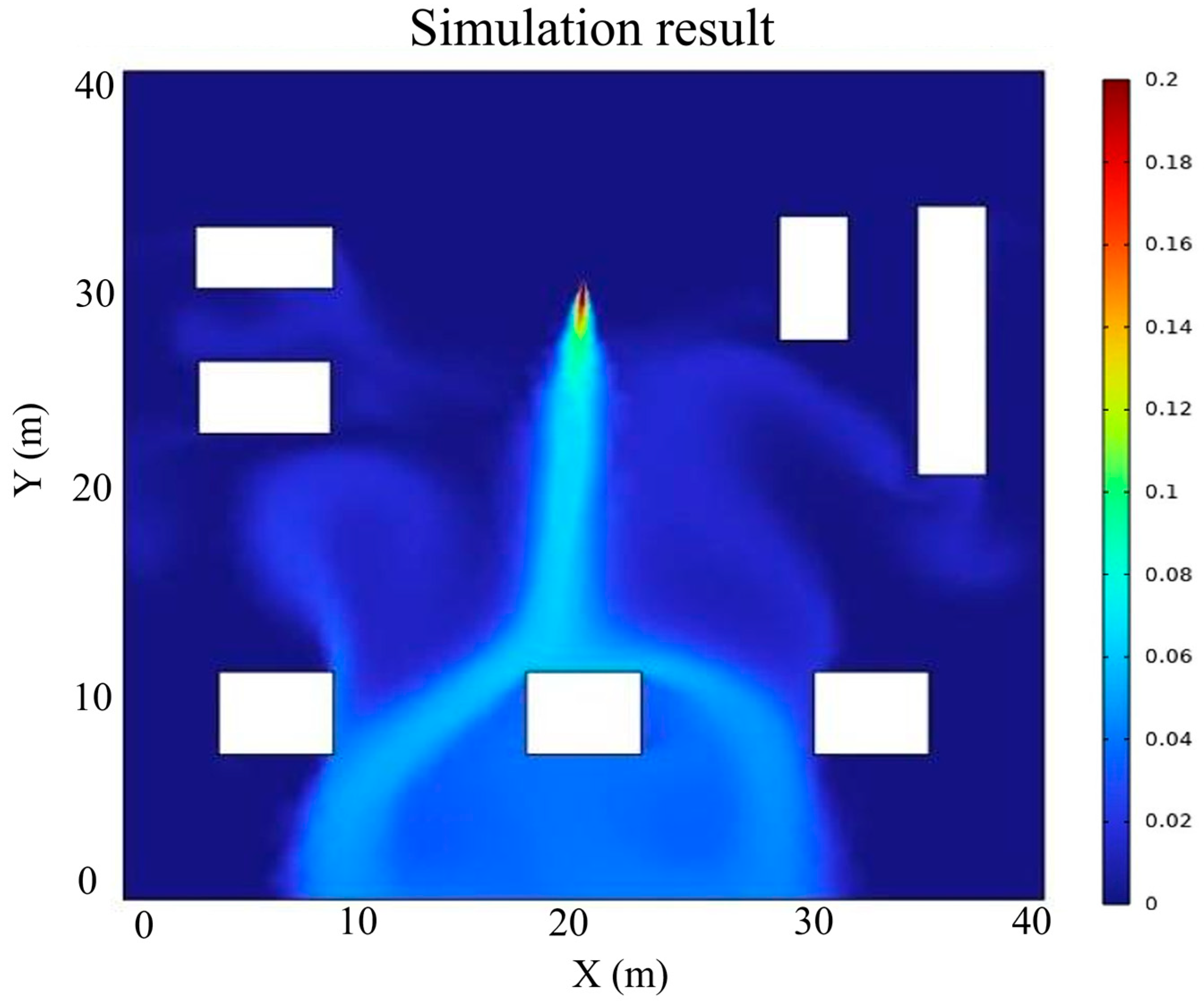
In this study, COMSOL6.4 simulation software was used to systematically simulate the natural gas leakage and dispersion process with obstacles, based on the $k-\epsilon$ turbulence model coupled with the mass transfer equation. A $40 \mathrm{m} \times 40 \mathrm{m}$ two-dimensional plane was adopted as the computational domain. The leakage hole diameter was set to 10 cm, the leakage source coordinate was (20, 30), the leakage rate was 3 kg/s, and the wind speed was 2 m/s. The simulation results are shown in Figure 3. Obstacles enhance the turbulence intensity of the gas. When blocked by obstacles during diffusion, the gas forms unique concentration distributions around obstacles, such as gas accumulation and delayed diffusion in the wake region. On the leeward side of obstacles, the gas flows around obstacles and forms vortices and local gas accumulation, leading to uneven concentration distributions.

Figure 3. Computational fluid dynamic simulation result.

The CFD simulation was used to obtain the gas concentration distribution in the monitoring region. The monitoring area was discretized into grid cells, and the concentration-time information of each grid cell was extracted. Based on the simulated concentration field, three risk indicators were obtained: peak concentration, hazardous concentration duration, and leakage probability. These indicators were then normalized and weighted to construct the comprehensive risk index. Parameter settings for simulation in Table 2.

Table 2. Parameter settings for simulation.

Category	Parameter	Setting
CFD simulation domain	Computational domain	40 m × 40 m (2D)
	Obstacle setting	Rectangular buildings
	Leakage source location	(20, 30)
	Leakage rate	3 kg/s
	Leak hole diameter	0.10 m
	Wind speed	2 m/s
	Wind direction	Uniform
CFD solver settings	Solver type	Pressure-based solver
	Flow model	k–ε turbulence model
	Pressure–velocity coupling	SIMPLE algorithm

It should be noted that the numerical benchmark case in this work adopts fixed meteorological and leakage parameters, including a uniform wind speed of 2 m/s, a fixed leakage rate of 3 kg/s and a single leakage position, which is designed to serve as a representative 2D obstacle-containing benchmark to fully demonstrate the integrated technical route of CFD risk mapping, NSGA-II multi-objective layout optimization and particle filter source inversion. Systematic parametric analysis covering variable wind speeds, wind directions and leakage flow rates requires massive additional CFD simulation cases, which will greatly expand the research scope and computational burden of the current manuscript, so such multi-condition comparative tests are not carried out in this paper. Nevertheless, the proposed optimization framework has strong generalization ability. When facing different wind fields or leakage working conditions, researchers only need to reconstruct the regional risk weight map by updating CFD simulation parameters, and the subsequent NSGA-II layout solving and particle filter source term estimation modules can be completely reused without structural modification of the algorithm.

3.2. Area Risk Classification Results

Based on the above case, the detection area is discretized into regular grid cells of $0.2 \mathrm{m} \times 0.2 \mathrm{m}$. Indexes including peak concentration, duration of gas concentration within $5\text{–}15\%$, and leakage probability (i.e., leakage frequency under each scenario) at each grid point are extracted. The weighted risk value of each grid node under different leakage scenarios is calculated and taken as the comprehensive risk index $R_i$. Obstacles are assigned zero risk weight and are not considered as coverage targets. However, they significantly influence gas dispersion patterns, leading to high-risk accumulation zones in surrounding regions. Therefore, sensor efficiency is evaluated based on risk-weighted coverage rather than geometric coverage.

$$R_i=w_1\cdot C_i+w_2\cdot T_i+w_3\cdot P_i$$

(7)

In the formula, $R_i$ is the comprehensive risk index, $C_i$ is the normalized peak concentration, $T_i$ is the normalized duration when the gas concentration ranges from 5% to 15%, and $P_i$ is the leakage probability. $w_1$, $w_2$, and $w_3$ are the weights of peak concentration, duration, and leakage probability, respectively.

The weights of the three risk indicators were determined using the analytic hierarchy process (AHP). The selected indicators include peak concentration, hazardous concentration duration, and leakage probability. First, a pairwise comparison matrix was established according to the relative importance of the three indicators in gas leakage risk assessment. The judgment matrix is expressed as:

$$A=\left[\begin{array}{ccc}1& 0.837& 1.714\\ 1.194& 1& 2.048\\ 0.583& 0.488& 1\end{array}\right]$$

(8)

where the three rows and columns correspond to peak concentration, hazardous concentration duration, and leakage probability, respectively. The priority vector was calculated by normalizing the eigenvector corresponding to the maximum eigenvalue of the judgment matrix.

The weights are determined by the analytic hierarchy process, with values of 0.36, 0.43, and 0.21.

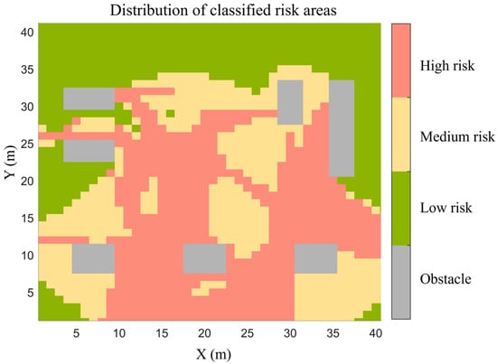
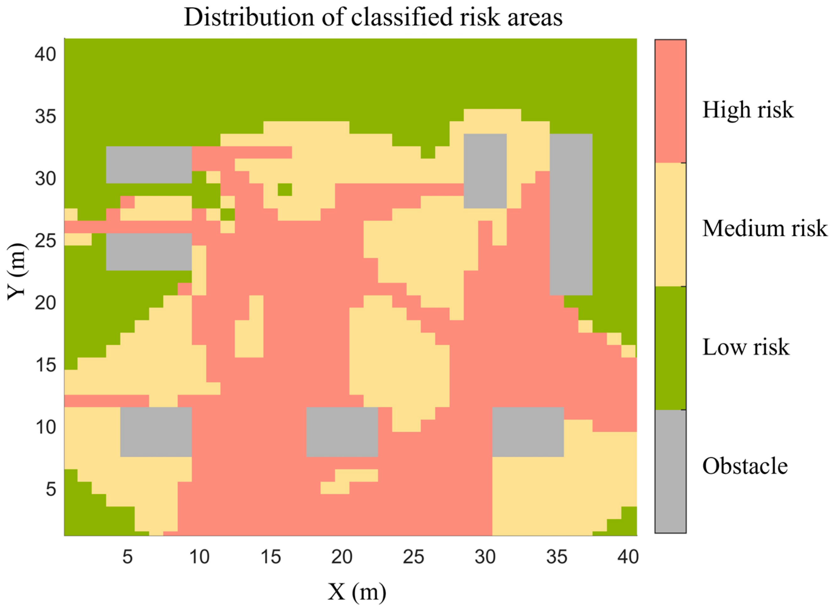
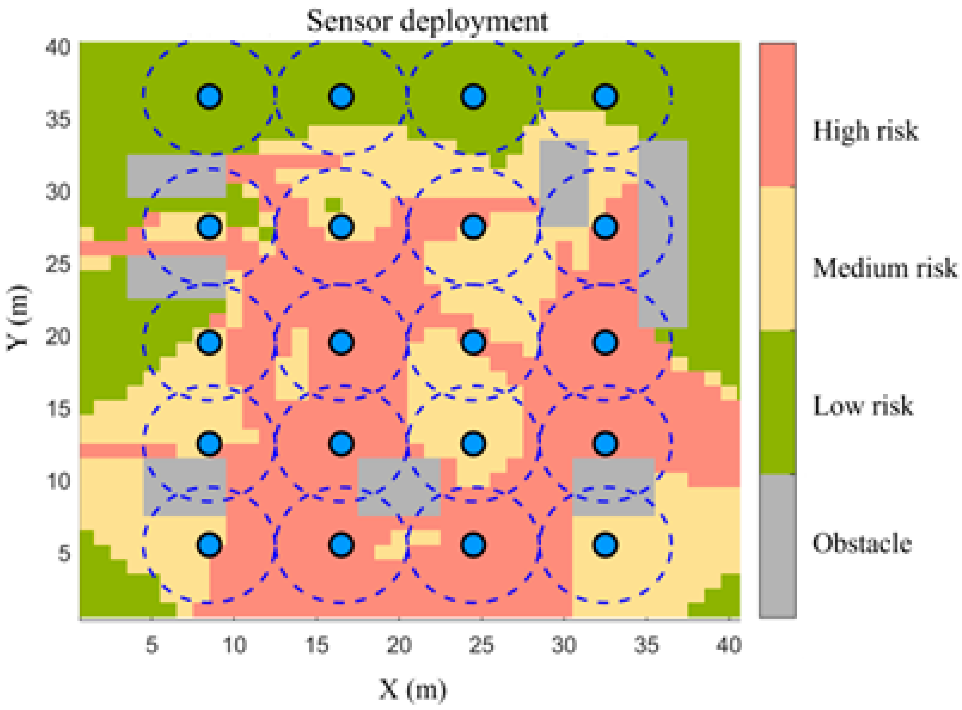
Then, the statistical quantile method is applied to determine the risk level thresholds. In this paper, the 30% and 60% percentiles are selected as the thresholds for low-medium risk and medium-high risk, respectively. Accordingly, the risk index is divided into three risk levels: low, medium, and high. Finally, a risk level matrix is constructed using a spatial interpolation algorithm to realize risk classification of the monitoring area. Weights are assigned to different risk level regions: the weight of obstacles is 0, low-risk is 1, medium-risk is 2, and high-risk is 4. The risk classification of the monitoring area is shown in Figure 4.

Figure 4. Area risk classification.

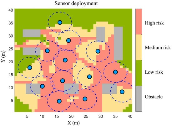
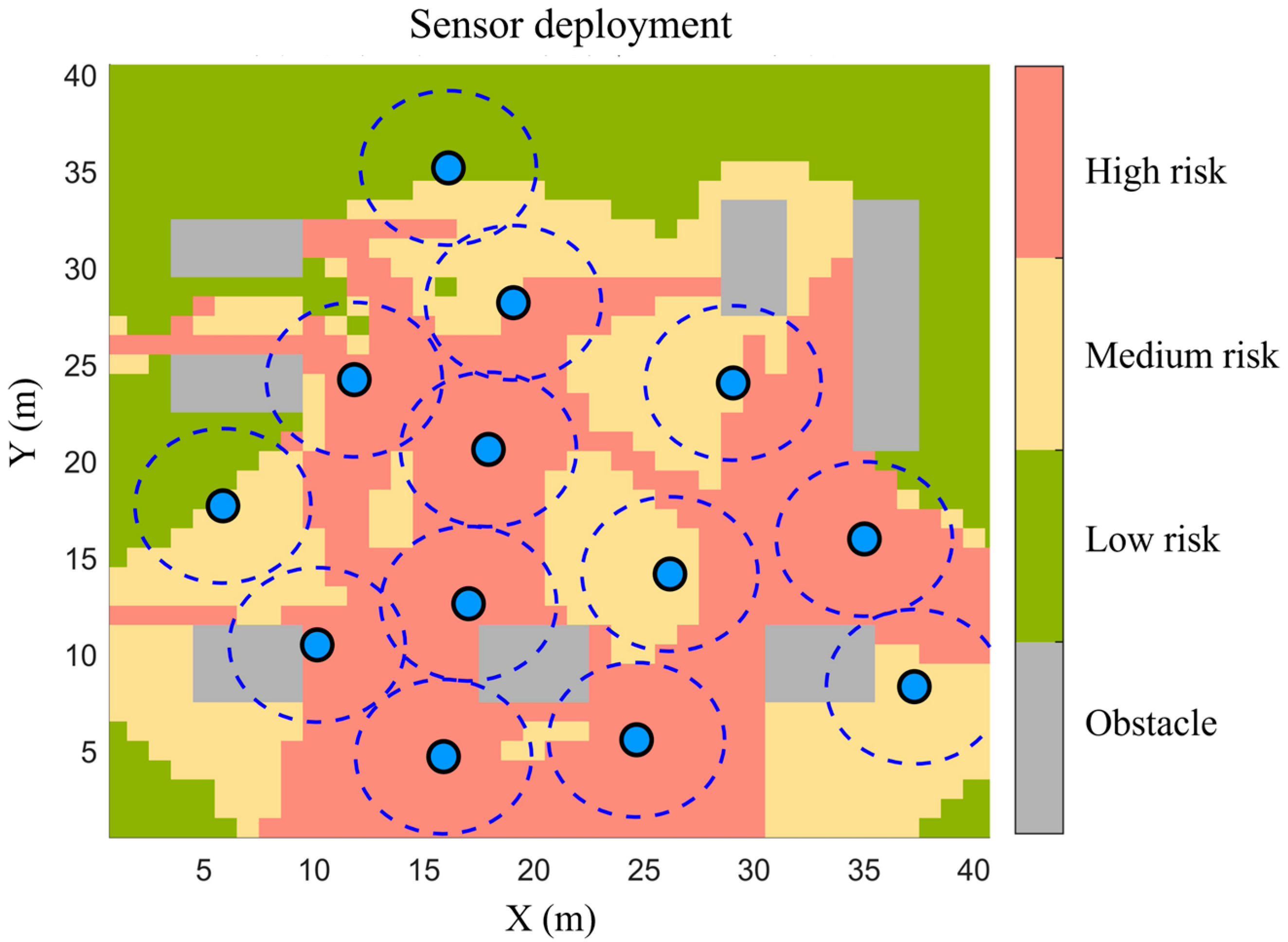
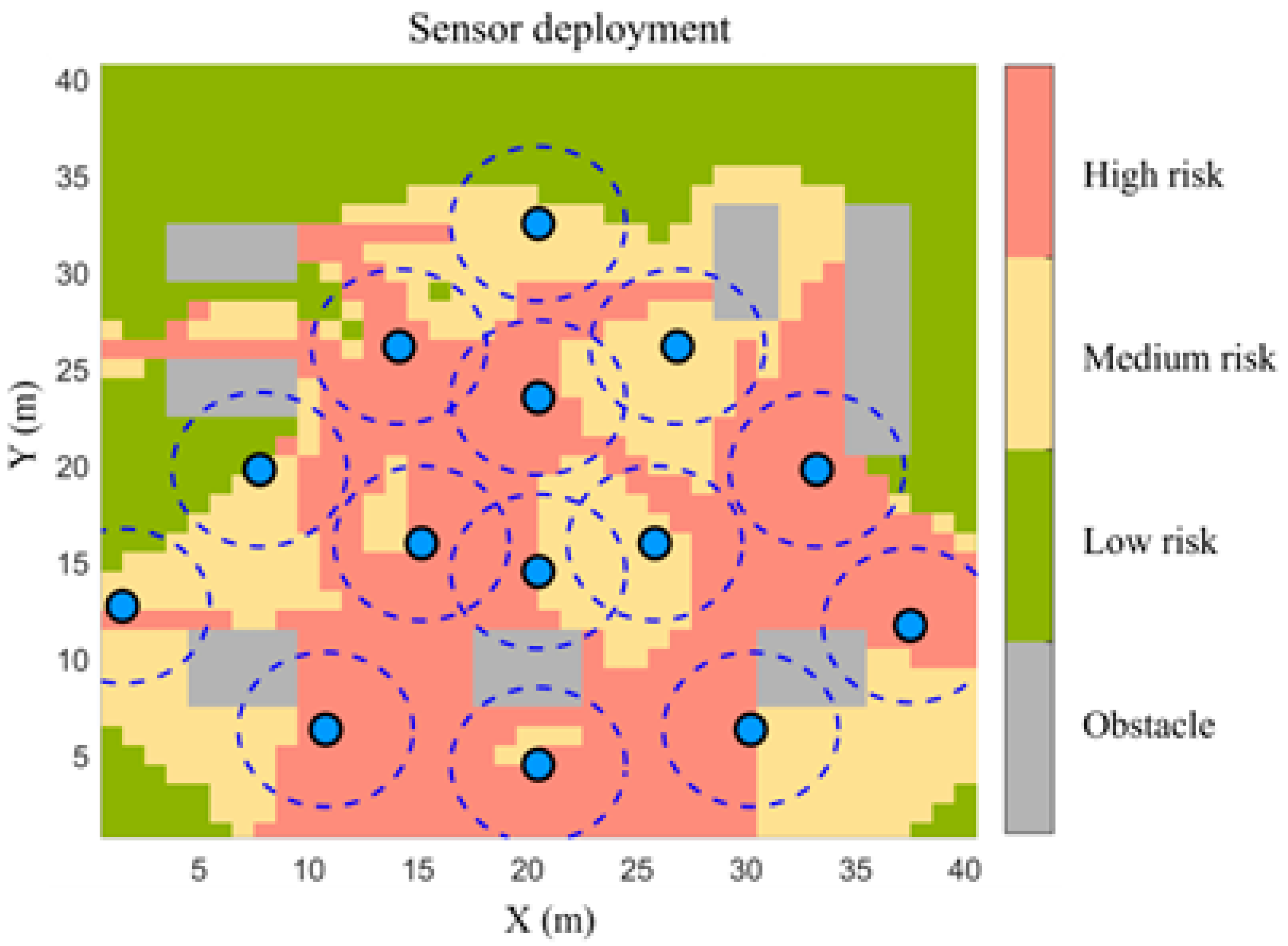
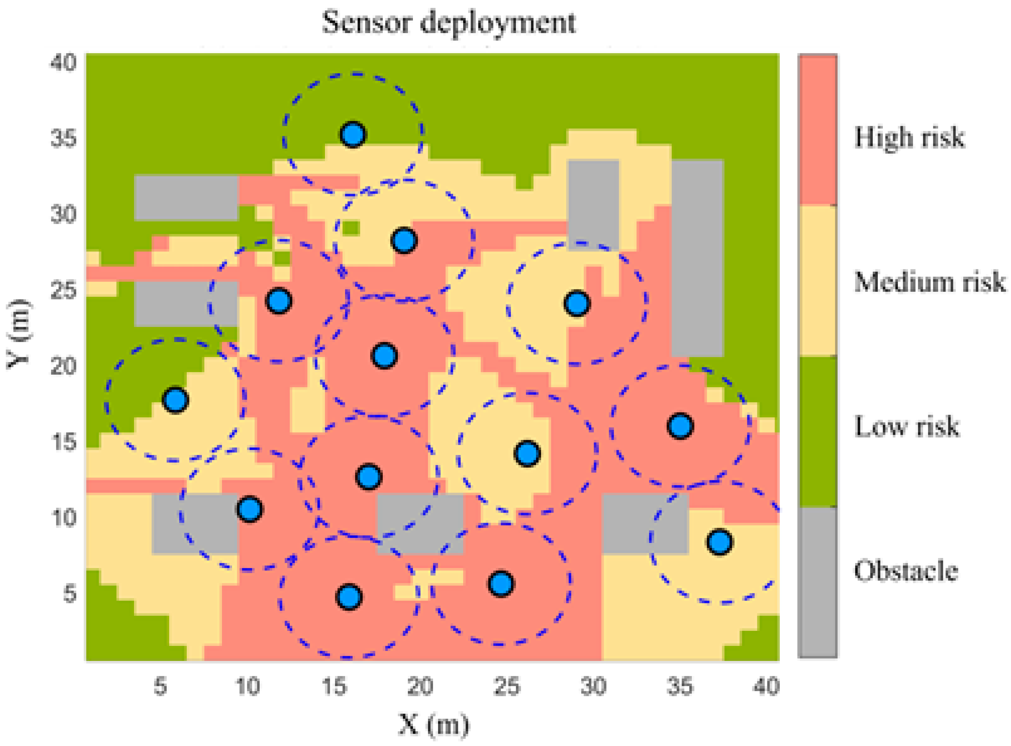
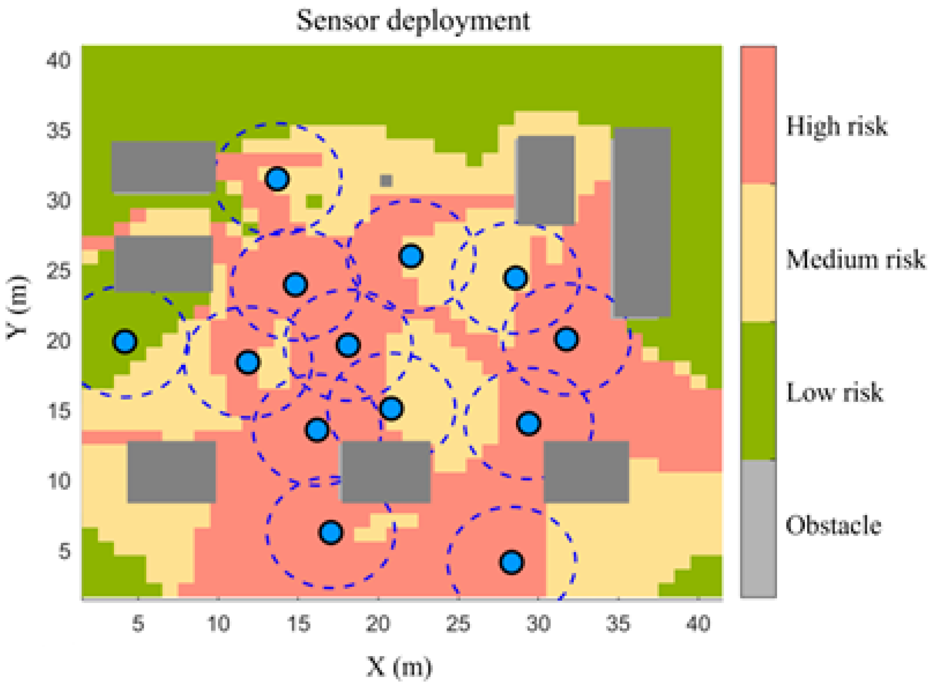
In this paper, the maximum number of sensors is set to no more than 20, with a sensing radius of 4 m for each sensor. The NSGA-II is adopted to continuously adjust the sensor positions through operations such as selection, crossover, and mutation, so as to balance the coverage of risk areas and the economic cost of sensor deployment. Finally, the solution with the relatively highest coverage rate is selected from the solution set. The optimized sensor layout is shown in Figure 5. The blue solid dots represent sensor positions, and the blue dashed circles indicate the coverage range of each sensor.

Figure 5. NSGA-II optimized layout.

The computational complexity of the proposed NSGA-II-based sensor layout optimization mainly comes from fitness evaluation, non-dominated sorting, and crowding distance calculation. For a population size of P, number of objectives M, number of monitoring grid cells G, and number of sensors N, the fitness evaluation has an approximate complexity of when direct coverage calculation is used. The non-dominated sorting procedure has a complexity of approximately, and the crowding distance calculation has a complexity of approximately.

Since the sensor layout optimization is an offline design procedure, the computational burden does not affect real-time monitoring after deployment. In this study, the population size and maximum number of generations were selected to balance optimization quality and computational cost. During iteration, the Pareto front gradually becomes stable, and the improvement in risk-weighted coverage becomes limited after repeated generations. Therefore, the maximum generation number and the stability of the Pareto solution set were used as termination criteria.

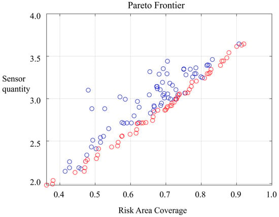
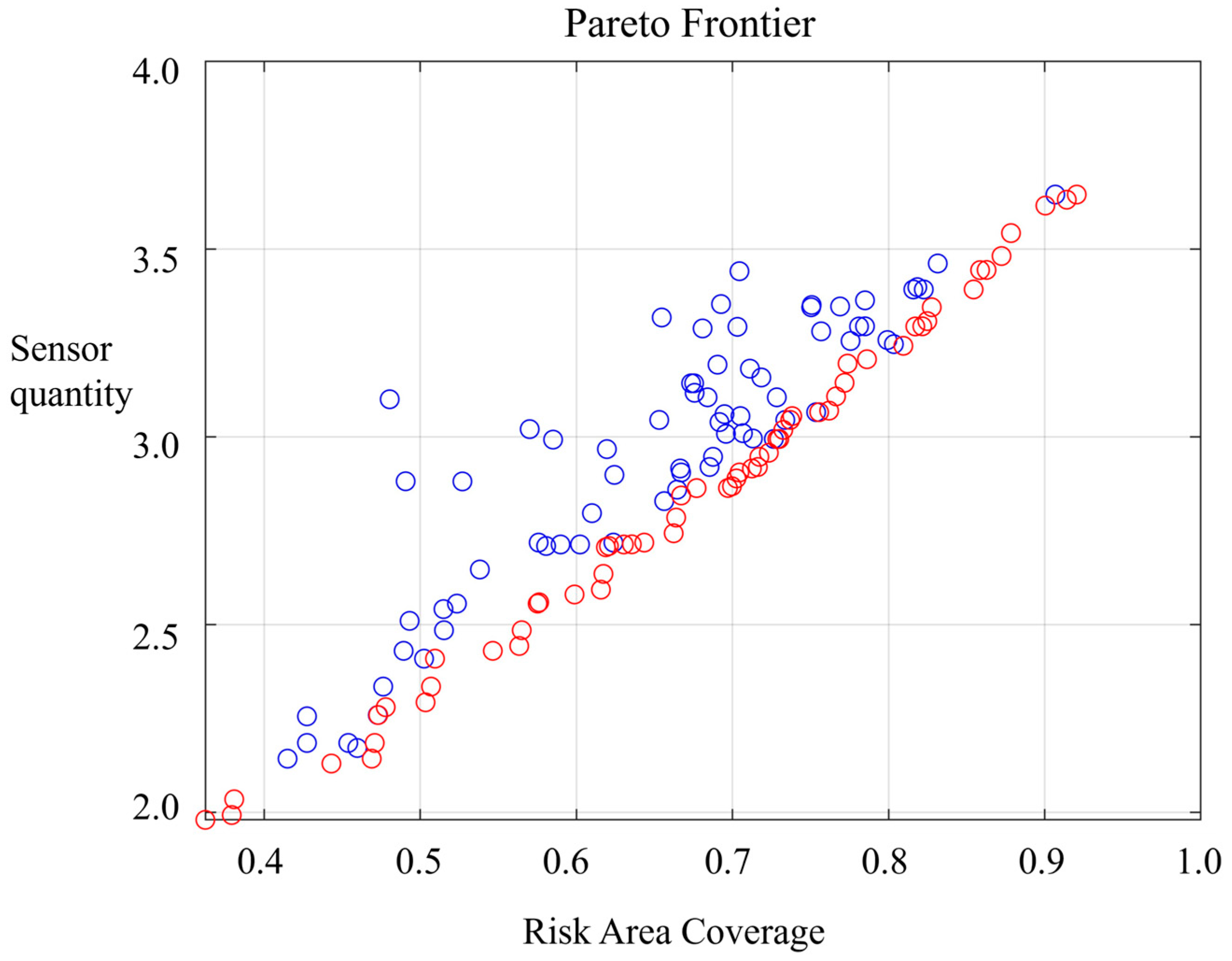
It can be seen from the Pareto front that the points are clustered along an approximate Pareto frontier curve, as shown in Figure 6. This indicates that with a limited number of sensors, the solution set exhibits typical non-dominated characteristics, reflecting the multi-objective trade-off between risk area coverage and resource constraints. It can be intuitively observed from the sensor layout distribution that the sensor network optimized by the NSGA-II exhibits significant spatial uniformity and achieves almost full coverage of high-risk areas. This demonstrates that the NSGA-II can effectively deploy sensors in key regions to improve overall coverage and monitoring performance.

Figure 6. Pareto frontier.

3.3. Particle Filter Results

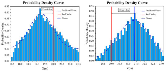
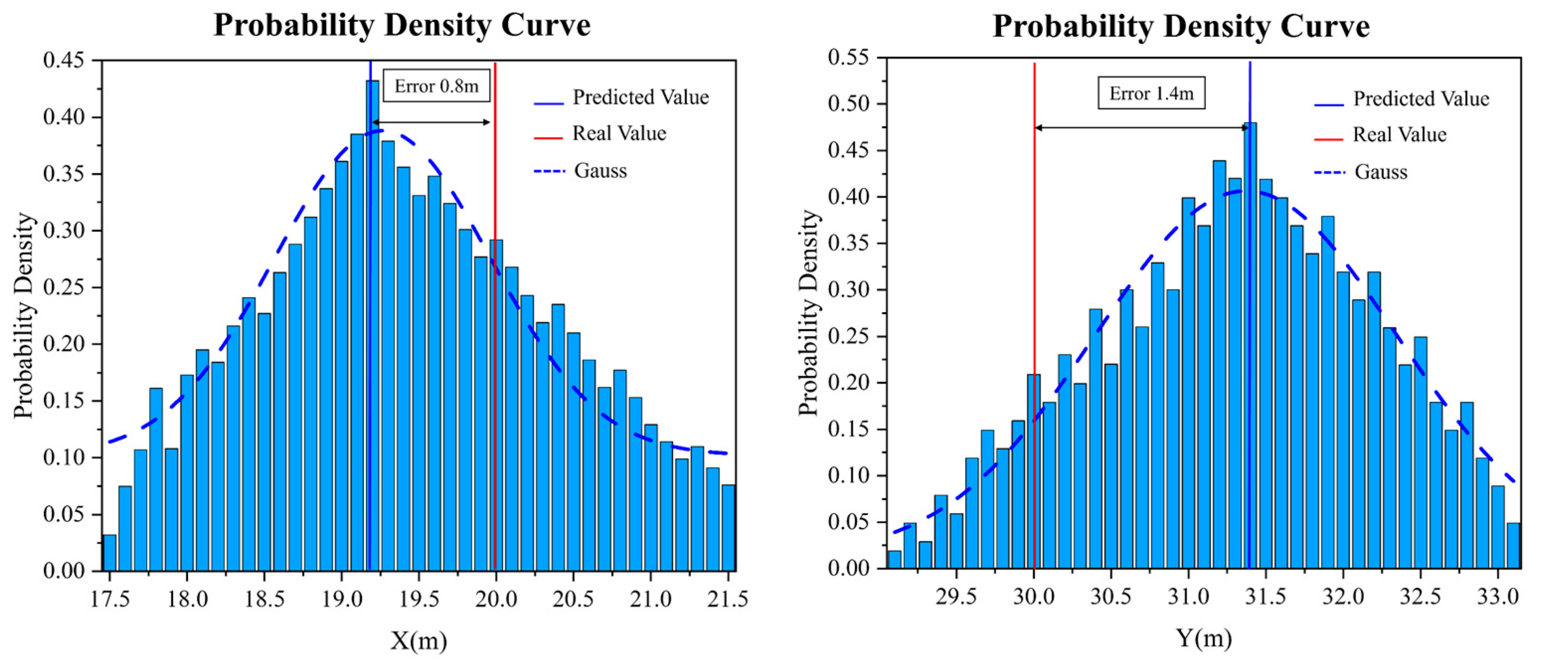
Figure 7 further illustrates the uncertainty distribution of the estimation results using a histogram. It can be observed that the localization errors in both X and Y directions are within 1.5 m. The proposed method can not only yield a single estimated value of leakage source parameters but, more importantly, can also derive the full posterior probability distribution. Meanwhile, it can also be observed that the high-probability regions in the histogram are mostly concentrated near the estimated position. This feature better satisfies the requirements of uncertainty quantification in practical engineering applications.

Figure 7. Posterior probability distribution of leakage source coordinates.

3.4. Comparison with Various Sensor Layout Methods

To evaluate the quality of the Pareto solution set, the Hypervolume indicator is used to comprehensively assess the convergence and diversity of the solution set. The Hypervolume indicator [24,25] balances convergence and diversity by quantifying the coverage volume of the solution set in the objective space. Since it does not require the true Pareto front, the Hypervolume indicator is widely adopted in engineering optimization design. The formula for the Hypervolume indicator is given as follows:

$$HV\left(S,r\right)=Volume\left({\bigcup }_{s\in S}\left[s_1,r_1\right]\times \left[s_2,r_2\right]\times \cdots \times \left[s_n,r_n\right]\right)$$

(9)

where $n$ is the number of objectives, and $s$ is a solution in the solution set $S$. Each solution $s$ corresponds to a hypercube whose vertices are defined by $s$ and the reference point $r$. In this section, the reference point is selected as the maximum value of each objective function plus a 5% offset to ensure that all solutions dominate the reference point.

Table 3 compares the performance of sensor layouts under different optimization algorithms. It can be seen from the table that compared with the MOPSO, the NSGA-II achieves higher coverage efficiency with fewer sensors. Its Hypervolume indicator is much higher than that of MOPSO, indicating that NSGA-II achieves a better balance between convergence and diversity of the solution set. Benefiting from the non-dominated sorting mechanism and crowding distance calculation, NSGA-II can effectively maintain the diversity and convergence of the solution set in sensor layout optimization. The MOPSO algorithm uses the same number of sensors as NSGA-II, but achieves a lower risk area coverage ratio. This is because the inertia mechanism in MOPSO may lead to uneven distribution of the solution set, thus degrading the risk area coverage performance.

Table 3. Comparison of sensor placement results under different optimization algorithms.

Sensor Layout Optimization Algorithm	Number of Sensors	Risk Area Coverage Ratio	Hypervolume Indicator
NSGA-II	13	78%	0.52
MOPSO	13	70%	0.43

Table 4 shows the comparison of gas leakage source estimation results under different sensor layouts. It can be seen from the table that after optimization by the non-dominated sorting genetic algorithm (NSGA-II), the accuracy of gas source estimation is greatly improved, and the localization error is reduced by approximately 44% compared with traditional layouts (grid layout and circular layout).

Table 4. Estimation results of source items under different sensor layouts.

Gas Sensor Layout		True Position of Gas Leakage Source	Estimated Position of Gas Leakage Source	Localization Error
Grid layout		(20, 30)	(18.69, 32.51)	2.83 m
Circular arc layout		(20, 30)	(18.95, 32.43)	2.64 m
NSGA-II Optimized layout		(20, 30)	(19.79, 31.57)	1.58 m
MOPSO Optimized layout		(20, 30)	(18.94, 32.01)	2.27 m
GA Optimized layout		(20, 30)	(18.62, 31.93)	2.37 m

Compared with MOPSO and GA, the source localization error after NSGA-II optimization is reduced by 0.304 and 0.333, respectively. This is because NSGA-II can effectively balance multiple optimization objectives through non-dominated rank and crowding distance comparison, avoiding the algorithm from falling into local optima. Although the MOPSO has a fast convergence speed, it relies heavily on collaboration among particles and has a weak ability in handling multi-objective problems, being easily affected by inertia weight and learning factors. The GA can only optimize a single objective, so it needs to assign weights to the multi-objective function and transform it into a single-objective function. This leads to excessive dependence on weight selection, which affects the sensor layout optimization.

Compared with traditional grid and circular arc layouts, the NSGA-II optimized layout places more sensors in high-risk regions derived from CFD simulation. These regions usually correspond to higher concentration, longer hazardous duration, and higher leakage occurrence probability. Therefore, under the same number of sensors, the NSGA-II optimized layout is expected to provide earlier leakage detection. However, detection time is not directly used as an optimization objective in this study. The main focus of this work is to balance risk-weighted coverage, deployment cost, and source localization accuracy. Quantitative detection-time optimization will be further investigated in future work.

4. Conclusions

In this study, a multi-objective optimization method is adopted to optimize the sensor layout for node deployment in fixed sensor networks. Hazardous areas are demarcated based on CFD simulation data in obstacle-present scenarios, with the maximization of risk area coverage and the minimization of sensor quantity set as the dual optimization objectives. The non-dominated sorting genetic algorithm is then applied to optimize the node distribution of the sensor network. Furthermore, the sensor layout results obtained from this method are compared with those generated by the multi-objective particle swarm optimization algorithm and the genetic algorithm.

The multi-objective optimization method for sensor layout based on NSGA-II proposed in this study can achieve precise coverage of high-risk areas in the monitoring region under the constraint of sensor quantity. With 13 sensors, a risk area coverage rate of 78% is achieved, representing an 8-percentage-point increase compared with the MOPSO algorithm using the same number of sensors. Moreover, the hypervolume indicator of its Pareto solution set reaches 0.52, which is much higher than 0.43 of the MOPSO algorithm. This demonstrates superior clustering performance, convergence and diversity of the solution set, and effectively balances the monitoring coverage of high-risk areas and the economic cost of sensor deployment.

The application of the NSGA-II-optimized sensor layout to particle filter-based natural gas leakage source term inversion significantly improves the leakage source localization accuracy, yielding a localization error of only 1.58 m. This represents an approximate 44% reduction in error compared with traditional grid and circular arc layouts, and a 30.4% and 33.3% decrease relative to the layouts optimized by the MOPSO and GA algorithms, respectively.

In addition, there exists a limitation in this study: the validation of the sensor layout optimization and source term estimation method is only carried out under a single fixed meteorological and leakage scenario. Future research will carry out multi-condition parametric analysis, including variable wind speeds, wind directions and different leakage rates, to quantify the influence of meteorological and leakage parameters on risk distribution and optimal sensor deployment schemes.

References

- Wang, X.; Zhang, D. Inverse identification of multiple contaminant sources and pollution states using future spatial-temporal information. J. Clean. Prod. 2021, 289, 125790. [Google Scholar] [CrossRef] [Scilit]
- Ni, C.; Lang, Z.; Wang, B.; Li, A.; Cao, C.; Du, W. Data-driven source term estimation of hazardous gas leakages in complex chemical industrial parks. Comput. Chem. Eng. 2026, 206, 109530. [Google Scholar] [CrossRef] [Scilit]
- Dong, J.; Wang, B.; Wang, X.; Cao, C.; Chen, S.; Du, W. Optimization of sensor deployment sequences for hazardous gas leakage monitoring and source term estimation. Chin. J. Chem. Eng. 2023, 56, 169–179. [Google Scholar] [CrossRef] [Scilit]
- Jing, Q.; Song, X.; Sun, B.; Li, Y.; Zhang, L. Efficient estimation of natural gas leakage source terms using physical information and improved particle filtering. Reliab. Eng. Syst. Saf. 2025, 260, 110989. [Google Scholar] [CrossRef] [Scilit]
- Ni, C.; Lang, Z.; Wang, B.; Li, A.; Cao, C.; Du, W. Source term estimation of hazardous gas leakages under turbulent atmospheric transport dispersion scenarios. Chin. J. Chem. Eng. 2025, 88, 222–238. [Google Scholar] [CrossRef] [Scilit]
- Benavides-Serrano, A.J.; Mannan, M.S.; Laird, C.D. A quantitative assessment on the placement practices of gas detectors in the process industries. J. Loss Prev. Process Ind. 2015, 35, 339–351. [Google Scholar] [CrossRef] [Scilit]
- Cen, K.; Yao, T.; Wang, Q.; Xiong, S. A risk-based methodology for the optimal placement of hazardous gas detectors. Chin. J. Chem. Eng. 2018, 26, 1078–1086. [Google Scholar] [CrossRef] [Scilit]
- Legg, S.W.; Wang, C.; Benavides-Serrano, A.J.; Laird, C.D. Optimal gas detector placement under uncertainty considering Conditional-Value-at-Risk. J. Loss Prev. Process Ind. 2013, 26, 410–417. [Google Scholar] [CrossRef] [Scilit]
- Legg, S.W.; Benavides-Serrano, A.J.; Siirola, J.D.; Watson, J.P.; Davis, S.G.; Bratteteig, A. A stochastic programming approach for gas detector placement using CFD-based dispersion simulations. Comput. Chem. Eng. 2012, 47, 194–201. [Google Scholar] [CrossRef] [Scilit]
- Zhou, C.; Zhang, B.; Qiao, S.; Mu, C. A stochastic programming approach for the optimization of gas detector placement in offshore platforms. Ocean Eng. 2019, 187, 106223. [Google Scholar] [CrossRef] [Scilit]
- Oleynik, A.; García-Ibáñez, M.I.; Blaser, N.; Omar, A.; Alendal, G. Optimal sensors placement for detecting CO2 discharges from unknown locations on the seafloor. Int. J. Greenh. Gas Control 2020, 95, 102951. [Google Scholar] [CrossRef] [Scilit]
- Rad, A.; Rashtchian, D.; Eghbal Ahmadi, M.H. Optimum placement of gas detectors considering voting strategy with different detection set points. J. Loss Prev. Process Ind. 2018, 55, 53–60. [Google Scholar] [CrossRef] [Scilit]
- Khorshidi, M.S.; Nikoo, M.R.; Taravatrooy, N.; Sadegh, M.; Al-Wardy, M.; Al-Rawas, G.A. Pressure sensor placement in water distribution networks for leak detection using a hybrid information-entropy approach. Inf. Sci. 2020, 516, 56–71. [Google Scholar] [CrossRef] [Scilit]
- Terman, M.S.; Kojouri, N.M.; Khalafi, H. Optimal placement of fixed in-core detectors for Tehran Research Reactor using information theory. Prog. Nucl. Energy 2018, 106, 300–315. [Google Scholar] [CrossRef] [Scilit]
- Kwak, D.; Jeong, J.; Shin, Y.; Lee, N.; Shin, D. Sensor placement optimization for fenceline monitoring of toxic gases considering spatiotemporal risk of the plant-urban interface. J. Taiwan Inst. Chem. Eng. 2022, 130, 103858. [Google Scholar] [CrossRef] [Scilit]
- Ma, D.; Ga, J.; Zhang, Z.; Wang, Q. An Improved Firefly Algorithm for Gas Emission Source Parameter Estimation in Atmosphere. IEEE Access 2019, 7, 111923–111930. [Google Scholar] [CrossRef] [Scilit]
- Lang, Z.; Wang, B.; Wang, Y.; Cao, C.; Peng, X.; Du, W.; Qian, F. A Novel Multi-Sensor Data-Driven Approach to Source Term Estimation of Hazardous Gas Leakages in the Chemical Industry. Processes 2022, 10, 1633. [Google Scholar] [CrossRef] [Scilit]
- Shui, Y.; Li, K.; Dang, J.; Zou, J.; Liu, Y. Optimization of hydrogen detector layout for leakage scenarios in hydrogen refueling stations. Int. J. Hydrogen Energy 2025, 178, 151499. [Google Scholar] [CrossRef] [Scilit]
- Liu, S.; He, R. Optimization of hydrogen sensor placement for hydrogen leakage monitoring in the fuel cell truck. J. Braz. Soc. Mech. Sci. Eng. 2023, 45, 193. [Google Scholar] [CrossRef] [Scilit]
- Feng, Y.; Lang, Z.; Jin, X.; Wang, B.; Cao, C. Physical field distribution-driven scenario reduction for gas sensor layout optimization within hydrogen-fueled gas turbine enclosures. Process Saf. Environ. Prot. 2026, 214, 109011. [Google Scholar] [CrossRef] [Scilit]
- Xie, Z.; Tang, J.; Yu, H.; Hu, Q.; Zhang, Y.; Meng, J.; Tian, G.; Li, R. Optimizing methane continuous monitoring networks in oil and gas fields: A multi-objective framework based on information theory. J. Clean. Prod. 2026, 552, 148010. [Google Scholar] [CrossRef] [Scilit]
- Chow, F.K.; Kosovic, B.; Chan, S. Source inversion for contaminant plume dispersion in urban environments using building-resolving simulations. J. Appl. Meteorol. Climatol. 2008, 47, 1553–1572. [Google Scholar] [CrossRef] [Scilit]
- Wang, S.; Li, L.; Cao, Z.; Li, H.; Fernandez, C.; Blaabjerg, F. Improved particle swarm-untracked particle filtering for accurate battery energy state estimation with the influence of multi-parameter varying temperature constraints in Inner Mongolia power station. Energy 2025, 341, 139492. [Google Scholar] [CrossRef] [Scilit]
- Braddstreet, L. The hypervolume indicator for multi-objective optimisation: Calculation and use. Ph.D. Thesis, The University of Western Australia, Perth, WA, Australia, 2011; pp. 10–17. [Google Scholar]
- Liu, Z.; An, K.; Tang, J.; Huo, J.; Chen, J. Current-Aware Informer and Reinforcement Learning enhanced Particle Filtering for mobile target localization in UASNs. Measurement 2026, 258, 119339. [Google Scholar] [CrossRef] [Scilit]
Disclaimer/Publisher’s Note: The statements, opinions and data contained in all publications are solely those of the individual author(s) and contributor(s) and not of MDPI and/or the editor(s). MDPI and/or the editor(s) disclaim responsibility for any injury to people or property resulting from any ideas, methods, instructions or products referred to in the content. |
© 2026 by the authors. Licensee MDPI, Basel, Switzerland. This article is an open access article distributed under the terms and conditions of the Creative Commons Attribution (CC BY) license.