Spatio-Temporal Assessment of a Live Fuel Moisture Content Monitoring Model from an Operational Perspective

Abstract

Live fuel moisture content (LFMC) is a key determinant of fuel flammability and forest fire danger; however, its operational monitoring remains challenging due to the limited spatial and temporal coverage of field measurements. This study aims to assess the operational suitability of a Random Forest-based methodology for LFMC estimation by extending a previously validated local-scale approach to a regional and multi-year context. Weighted average LFMC was modeled across 67 shrubland plots in the Valencian Region (eastern Spain) from 2017 to 2025 using Sentinel-2 spectral indices and aggregated meteorological variables consistent with prior research. Model performance was evaluated under spatially independent and combined spatio-temporal training–testing scenarios designed to approximate real-world wildfire monitoring conditions. Results show that the model exhibits good spatial transferability when applied to shrubland plots not used during training within the same temporal domain, while temporal extrapolation is more limited and dependent on the stability of climatic conditions represented in the training data, with a marked decline in performance under changing temperature and precipitation regimes. These findings highlight key drivers of LFMC prediction, identify validation strategies under operational constraints, and contribute to the development of scalable monitoring approaches for wildfire danger assessment and fuel management in Mediterranean shrublands.

1. Introduction

Wildfires occur across regions worldwide, and their characteristics are increasingly influenced by climate change, fuel accumulation, and land-use transformations, which can shape their ecological, economic, and social outcomes [1,2,3]. These drivers are particularly pronounced in Mediterranean ecosystems, characterised by recurrent summer droughts and strong interannual climatic variability, where wildfires have intensified in frequency and severity over recent decades [4,5,6]. Reliable wildfire danger assessment is therefore essential for prevention, early warning, and operational fire management, requiring accurate monitoring of vegetation status and fuel conditions.

In Mediterranean-climate regions, shrublands play a central role in wildfire behaviour because they constitute one of the dominant fuel types and are characterised by high horizontal continuity and pronounced seasonal drying. These characteristics favour fire propagation across the landscape, while the vertical arrangement of shrubs and understory vegetation may facilitate transitions from surface to crown fires by acting as ladder fuels [7,8]. Recent studies have further shown that ladder fuels are more closely associated with wildfire severity than canopy fuel loads alone [9]. This is particularly relevant in Mediterranean ecosystems, where crown fire initiation has been linked to intense surface fires capable of generating direct flame contact with the canopy [10]. Consequently, understanding and monitoring the moisture dynamics of shrubland fuels is essential for improving wildfire danger assessment and supporting operational fire management.

Among the biophysical variables influencing fire ignition, spread, and behaviour, live fuel moisture content (LFMC) is recognised as a key determinant of fuel flammability [11,12,13,14]. LFMC affects heat release, ignition thresholds, combustion efficiency, and rate of spread, with lower values strongly associated with extreme fire behaviour [15,16,17]. However, traditional LFMC estimation based on destructive sampling is labour-intensive, spatially limited, and temporally infrequent [18], motivating the development of remote sensing approaches capable of landscape-scale monitoring.

Optical remote sensing has long been used to estimate LFMC by exploiting vegetation spectral responses to water content [19,20,21]. Vegetation indices such as NDVI, NDII, MSI, EVI, and chlorophyll-related indices have shown sensitivity to LFMC across shrublands and forest ecosystems [12,22,23,24], while radiative transfer modelling has improved understanding of spectral–moisture interactions [13,25]. Meteorological drivers—including precipitation, temperature, vapour pressure deficit (VPD), and relative humidity—further modulate LFMC through plant–atmosphere water exchange and soil–plant hydraulic stress [26,27,28].

Machine learning (ML) approaches, particularly Random Forest, Gradient Boosting, and neural networks, have recently improved LFMC estimation by modelling nonlinear interactions among spectral and meteorological variables [29,30,31]. Studies have demonstrated promising results across Mediterranean zones [32,33]. Yet, concerns remain regarding the spatial and temporal transferability of empirical and ML-based LFMC models, especially when applied beyond the environmental domain where they were trained [34].

Recent research emphasises the need for operational LFMC products designed for real-time wildfire danger assessment. Watt et al. [35] describe a roadmap for near-real-time LFMC monitoring, highlighting sensor complementarity, data fusion, and model integration into fire danger rating systems. Benali et al. [36] present a national operational LFMC product demonstrating the potential for real-time fire-risk applications. Transferability studies by Marino et al. [37] reveal substantial limitations when empirical LFMC models are applied across heterogeneous landscapes. The need for spatial and temporal independent validation schemes is evident to realistically assess model robustness and carry out its operational deployment.

Mediterranean shrublands exhibit strong spatial and phenological heterogeneity, which complicates LFMC modelling at regional scales [38]. Local-scale studies using Sentinel-2 spectral indices and meteorological variables have demonstrated the potential to achieve accurate LFMC predictions in these ecosystems. For example, the study described in [31] calibrated models using field observations collected between June 2020 and November 2021 across 43 shrubland plots distributed within 13 zones of the Valencian Region (eastern Spain). Although this and similar works confirm the suitability of combined spectral and meteorological predictors for LFMC estimation, most studies to date are based on relatively short observation periods and limited site networks. Consequently, important questions remain regarding the scalability of these approaches and their reliability when applied over longer time periods and across broader spatial extents.

Building upon these previous findings, the Random Forest (RF) framework adopted in the present study is based on the methodology developed in [31], where RF demonstrated robust performance for LFMC estimation in Mediterranean shrublands owing to its ability to represent the complex, non-linear relationships between spectral, meteorological, and environmental predictors. Likewise, TCARI was retained as the spectral predictor because its suitability for LFMC estimation in the study area had previously been demonstrated, owing to its sensitivity to chlorophyll content [39]. This sensitivity is particularly relevant in Mediterranean ecosystems, where variations in chlorophyll content are often associated with changes in vegetation health and water status under hydric stress. Building on this validated foundation, the present study further extends the modelling framework by introducing methodological refinements, including a logarithmic transformation of accumulated precipitation (ln(1 + p60)), the evaluation of an additional candidate predictor (vapour pressure deficit, VPD), and a substantially extended operational assessment through multi-year spatio-temporal validation.

Accordingly, the present study evaluates the operational robustness of this modelling framework using 67 shrubland plots across the Valencian Region during the period 2017–2025. Building upon a previously validated modelling framework enables direct assessment of model robustness while evaluating the methodological extensions introduced in the present study. Model robustness is assessed under spatially independent, temporally independent, and combined spatio-temporal validation scenarios designed to mimic real operational conditions. Specifically, the objectives of this study are to (i) analyse the accuracy of the Random Forest approach when extrapolating LFMC estimates to time periods not represented in the training dataset, and (ii) evaluate the robustness of the methodology when applied to spatially independent plots located at varying distances from those used for model training. This work contributes to the development of scalable LFMC monitoring tools to support wildfire danger assessment, fuel management, and early-warning systems in Mediterranean shrubland regions.

2. Materials and Methods

2.1. Study Area and Field Data

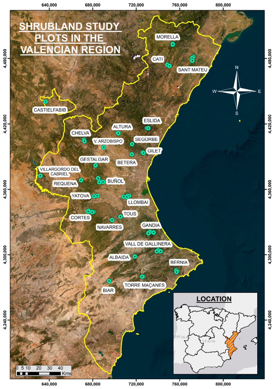
The field LFMC data used in this study are based on the same sampling campaigns and quality-control procedures implemented in earlier work by [31], in which field measurements were collected across 43 shrubland plots in the Valencian Region (eastern Spain). The same database, extended to include additional plots to reach 67 sites for the period 2017–2025 (see Figure 1), was adopted here.

The study area is characterised by typical Mediterranean climatic conditions, with hot, dry summers and mild winters, and is dominated by shrubland formations exhibiting strong spatial variability in structure, species composition, and moisture dynamics, making the region particularly suitable for analysing LFMC variability across environmental gradients. Live fuel moisture content was calculated using the standard gravimetric Method (1), as follows:

$$\mathrm{L}\mathrm{F}\mathrm{M}\mathrm{C}={\displaystyle \frac{W_f-W_d}{W_d}}\times 100$$

(1)

where $W_f$ is the fresh weight of the vegetation sample and $W_d$ is its dry weight after oven-drying to constant mass. For each plot and date of observation, the weighted average LFMC was computed using the fraction of canopy cover (FCC) of dominant species, following the approach adopted in previous studies [31,38,40]. This weighting procedure ensures that the contribution of each species to overall fuel moisture reflects its proportional presence in the plot. In its most recent version, the database includes revised and updated information on vegetation type and fraction of canopy cover (FCC).

2.2. Data Sources and Operational Infrastructure

The data used in this study are hosted on the SIGIF web platform (https://prevencionincendiosgva.es/HCVivo, last accessed: 7 January 2026), which corresponds to the Integrated Forest Fire Management System of the Government of the Valencian Region. This platform currently implements the linear LFMC estimation models developed in [38]. The existing data infrastructure has been leveraged to evaluate the performance of the Random Forest-based methodology, with the aim of assessing its potential to replace the operational linear models in future implementations. The database integrates spectral and meteorological data at a spatial resolution of 100 × 100 m, obtained through an automated system that retrieves and processes meteorological and spectral information on a daily basis at this resolution.

2.3. Predictor Variables and Preprocessing

Spectral and meteorological predictors were derived following a harmonised spatio-temporal framework designed for operational LFMC modelling. The initial predictor pool comprised 26 candidate variables representing spectral, meteorological, seasonal, geographic, and topographic information. These variables were derived from a dataset with daily temporal resolution based on field plot coordinates.

2.3.1. Spectral Variables

Spectral indices associated with vegetation water status and canopy structure, including EVI (Enhanced Vegetation Index), SAVI (Soil-Adjusted Vegetation Index), OSAVI (Optimized Soil-Adjusted Vegetation Index), NDVI (Normalized Difference Vegetation Index), RVI (Ratio Vegetation Index), VARI (Visible Atmospherically Resistant Index), SLA (Specific Leaf Area Index), ARVI (Atmospherically Resistant Vegetation Index), Vgreen (Green Vegetation Index), TCARI (Transformed Chlorophyll Absorption in Reflectance Index), NDMI (Normalized Difference Moisture Index), NMDI (Normalized Multi-band Drought Index), NDWI (Normalized Difference Water Index), MSI (Moisture Stress Index), and TCARI/OSAVI, were computed from atmospherically corrected Sentinel-2 Level-2A imagery through the Google Earth Engine (GEE) platform, following the methodology described in [40]. These indices capture leaf water absorption features, chlorophyll activity, and canopy stress conditions.

2.3.2. Meteorological Variables

Meteorological predictors were obtained from daily observations recorded at weather stations operated by the Spanish Meteorological Agency (AEMET). The original dataset included variables related to air temperature, relative humidity, and precipitation from nearby meteorological stations. To transfer these observations to all study plots, spatial interpolation was performed using the Meteoland package [41] in the R 4.5.1 software environment. This approach enables the estimation of meteorological conditions at unsampled locations by accounting for geographic coordinates (X–Y), elevation, slope, and terrain aspect, thereby generating plot-level predictors consistent with local topographic variability.

Specifically, the initial meteorological predictors were: t60 (mean daily air temperature averaged over the previous 60 days), p60 (cumulative precipitation over the previous 60 days), and HUmin15 (mean minimum daily relative humidity over the previous 15 days). Wind speed and direction were not included, as these variables were available from a more limited number of meteorological stations.

Although additional temporal windows of 7, 15, and 30 days were tested for averaging or accumulating these variables, the selected periods showed the strongest correlation with LFMC. These meteorological predictors were derived following the same data acquisition and preprocessing framework described in [31]. However, one of the original variables (cumulative precipitation during the 60 days preceding each field sample—p60) was modified for the present study. Cumulative precipitation was transformed using the natural logarithm of 1 + p60 (i.e., ln(1 + p60)) instead of using p60 directly. Applying this log transformation reduces the influence of extreme precipitation events and helps stabilise variance by moderating the rapid increase in p60 values during periods of intense rainfall, while the addition of a constant ensures numerical stability and allows the transformation to be applied consistently under zero-precipitation conditions. Furthermore, this study incorporated an additional variable: VPD (daily maximum vapour pressure deficit), which represents the difference between saturation vapour pressure and actual vapour pressure in the air. It is computed using daily maximum temperature and minimum relative humidity following the formulations presented in [42,43,44]. VPD is a key factor for understanding plant water stress, as high values indicate dry atmospheric conditions that can increase plant water demand. Therefore, it is strongly linked to LFMC dynamics. Moreover, this variable plays a critical role in the likelihood of large forest fires by acting as a primary driver of fuel aridity and atmospheric evaporative demand [45].

2.3.3. Seasonal and Spatial Predictors

Seasonality was represented using the sine and cosine of the day of year, while geographic coordinates (Xcoord, Ycoord) and topographic descriptors (altitude, slope, and aspect) were included to capture spatial gradients in LFMC dynamics. Topographic variables were derived from a 5 m resolution Digital Elevation Model (DEM) provided by the Institut Cartogràfic Valencià (ICV). The inclusion of these seasonal, spatial, and topographic predictors is based on the findings of [31,38], which indicate their important role in LFMC estimation.

2.4. Feature Selection, Validation, and Model Development Framework

To simplify models and reduce the risk of overfitting, a Forward Feature Selection (FFS) method was applied, consisting of training models using all possible combinations of two variables from the initial set of 26 predictors (15 spectral indices derived from satellite imagery, 4 meteorological, 2 seasonal, 2 spatial, and 3 topographic). Variables were then added iteratively, selecting at each step the variable producing the greatest reduction in prediction error. The selection procedure identified six key variables for estimating weighted LFMC: the TCARI spectral index, t60 (mean temperature over 60 days), ln(1 + p60), sine of day of year, cosine of day of year, and Ycoord (northing coordinate).

To evaluate model performance, a Leave-Location-Out Cross-Validation (LLOCV) framework was implemented. Unlike conventional random validation, which may produce overly optimistic error estimates due to spatial autocorrelation, LLOCV excludes an entire location (plot), including all observations across all dates for that location, at each iteration. This approach ensures that the results reflect the model’s ability to predict LFMC at spatially independent sites.

Model development and tuning were carried out in R, using the packages CAST (for FFS and LLOCV), caret (for training management), and randomForest (for implementing the Random Forest algorithm). The number of trees (ntree) was set to 500, while the mtry parameter (number of randomly selected variables at each split) was tuned interactively, starting from a value of 2 and selecting the value that minimised prediction error.

2.5. Definition of Specific Models

Models were developed to estimate weighted LFMC based on data collected during the period 2017–2025 across multiple shrubland plots in the Valencian Region. Model performance was evaluated using spatially independent, and spatio-temporally independent validation schemes, considering the three scenarios described below.

2.5.1. Scenario A

The Random Forest model was trained using all available shrubland samples collected between June 2020 and November 2021. This configuration mirrors the temporal setup of the previously published study [31], while extending the spatial coverage from the 43 plots originally used to 56 plots containing observations within that same training period. Among these 56 plots, 41 also include observations from periods outside the training interval. The complete database comprises 67 shrubland plots, of which 11 include observations only outside the training period and were therefore not considered in model development under this scenario, serving exclusively for spatio-temporally independent validation. This updated dataset is consistent with the spatial framework adopted by SIGIF from the year 2025 and described in Section 2.1. Model performance was evaluated under two temporally independent validation subsets: Validation A1, corresponding to backward temporal extrapolation using observations collected during 2017–2020, and Validation A2, corresponding to forward temporal extrapolation using observations collected during 2022–2025.

2.5.2. Scenario B

The model was trained using samples from the entire 2017–2025 period, selecting 80% of the shrubland plots for training and reserving the remaining 20% for validation. Plot selection was stratified to ensure representation of municipalities with multiple sampling sites in both subsets. Model evaluation was based exclusively on validation plots not used during training (spatially independent validation).

2.5.3. Scenario C

The temporal generalisation capacity of the Random Forest model was evaluated using a sequential year-by-year validation approach. For each evaluation year, the model was trained using only samples collected prior to that year and tested on samples from the corresponding year, which were not included in the training dataset (one-year spatio-temporally independent validation).

Together, the three validation scenarios described above test the ability of the models to predict LFMC in new locations and under varying climatic conditions. Within this context, the modelling framework integrates automated feature selection, spatial cross-validation, and explicit extrapolation assessment into a unified approach that mitigates overfitting and enhances model robustness when applied across heterogeneous Mediterranean shrubland environments.

2.6. LFMC Mapping

Cartographic LFMC estimates were generated for 14 July 2021 and 8 August 2022. Differences between field-measured and cartographically predicted LFMC were calculated for Scenario A, Scenario B, and the Random Forest model presented in [31], using 54 plots with field observations collected close to 14 July 2021, and 26 additional plots with observed values collected close to 8 August 2022. For the July 2021 comparison, field measurements ranged from 1 July to 29 July 2021, whereas for the August 2022 comparison, field observations ranged from 27 July to 23 August 2022.

Cartographic representation of LFMC was performed using the operational data infrastructure of the Integrated Forest Fire Management System (SIGIF), which provides spectral and meteorological predictors at a spatial resolution of 100 × 100 m across the Valencian Region. Using these inputs, the trained Random Forest models corresponding to Scenario A, Scenario B, and the model described in [31] were applied to generate spatially continuous LFMC prediction maps for the two selected dates. Spatial predictions were restricted to shrubland areas, consistent with the scope of the models, which were specifically developed for dense shrub fuel types: SH4 and SH5 [46], as defined in the official fuel models map of the Valencian Government (https://cjusticia.gva.es/es/web/prevencion-de-incendios/models-de-combustible; last accessed: 1 May 2026). In addition to the LFMC prediction maps, spatial representations of prediction error were generated to evaluate model performance under operational mapping conditions. Prediction error was calculated at each plot as the difference between the cartographically predicted LFMC and the corresponding field measurement. These differences were mapped at the plot locations to visualise the spatial distribution of model deviations.

Furthermore, to quantify systematic deviations between predicted and observed LFMC values, the Bias (BIAS) metric was calculated for each date and modelling scenario. BIAS was computed as the mean of the differences between predicted and field LFMC values across all plots considered for each cartographic comparison. This metric provides an aggregate measure of the tendency of the models to overestimate or underestimate LFMC under the climatic conditions represented on each mapping date.

3. Results

This section presents the performance of the Random Forest models for estimating weighted average live fuel moisture content (LFMC) in shrubland plots under three different training and testing scenarios. Although the final models were implemented using a reduced set of predictor variables (DOY_SIN, DOY_COS, ln(1 + p60), T60, Ycoord, and TCARI), the modelling process initially started from the 26 candidate predictors discussed in Section 2.4, including multiple spectral, meteorological, seasonal, geographic, and topographic variables. As described in Section 2.4, Forward Feature Selection was used to derive a reduced subset of predictors. Reducing the model to six predictors resulted in similar predictive accuracy while improving model parsimony, interpretability, and stability. The selected subset closely aligns with the key variables identified in [31], facilitating comparison with earlier work while maintaining a consistent and robust framework for evaluating model behaviour across spatial and temporal validation schemes.

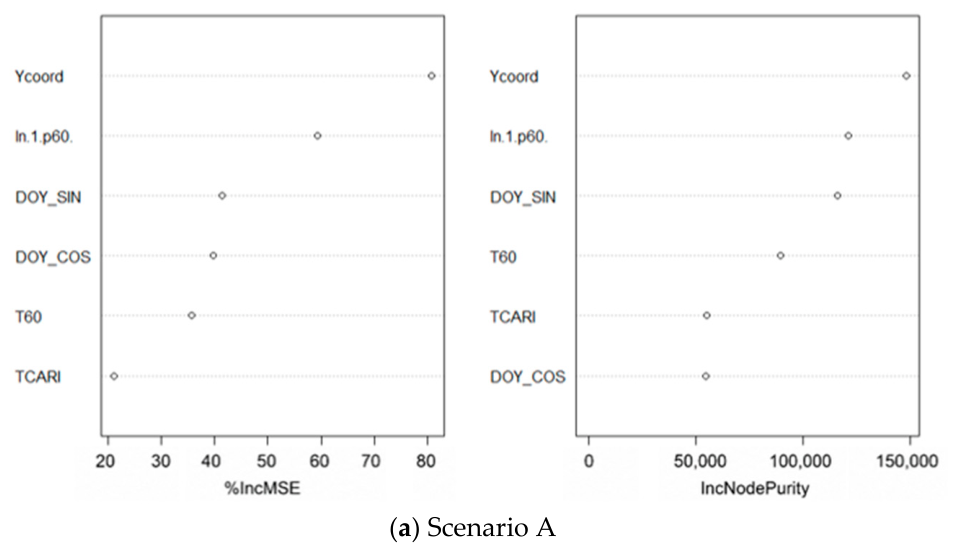
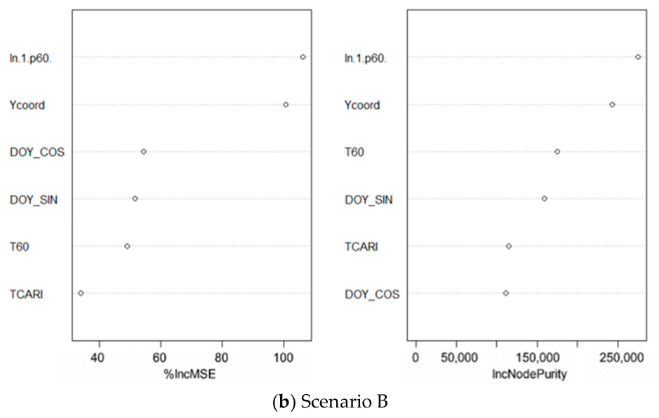
Figure 2 presents the analysis of the variable importance. For comparative purposes, the training datasets from Scenario A (samples collected between June 2020 and November 2021) and Scenario B (samples from the 2017–2025 period, selecting 80% for training) were used, allowing the variation in variable selection to be observed when using a smaller versus a larger training dataset, as shown in Figure 2a and Figure 2b, respectively. The validation results obtained with these scenarios are described in detail in Section 3.1 and Section 3.2.

3.1. Scenario A: Space–Time Extrapolation from a Fixed Training Period (2020–2021)

To facilitate comparison between the two temporal validation subsets (before and after that training period, respectively),

Table 1. Performance metrics derived during model development (2020–2021) and for independent testing scenarios: A1 (2017–2020) and A2 (2022–2025).

Dataset	No. Samples	R2 Adj (%)	RMSE	MAE
No. training plots: 56	1670	57.655	13.147	10.751
No. A1 testing plots: 36	699	58.796	10.265	8.444
No. A2 testing plots: 30	1404	39.524	18.271	15.499

summarises the performance metrics obtained for Scenario A under Validation A1 (2017–2020) and Validation A2 (2022–2025). This table provides an overview of model behaviour across temporally independent conditions, while detailed results for each validation subset are described in the following subsections. In this case, the model was evaluated on both plots that were included in the training dataset (but at different dates) and plots not used during training.

3.1.1. Validation A1: Testing on Earlier-Period Data (2017–2020)

The first validation subset consisted of samples collected between May 2017 and May 2020, corresponding to dates preceding the training period. Results, shown in Table 1, indicate a moderate predictive performance, with acceptable agreement between observed and predicted LFMC values. It should be noted that the performance metrics obtained during the model design were derived using leave-one-location-out cross-validation (LLOCV), ensuring that all samples from a given plot were excluded simultaneously during validation.

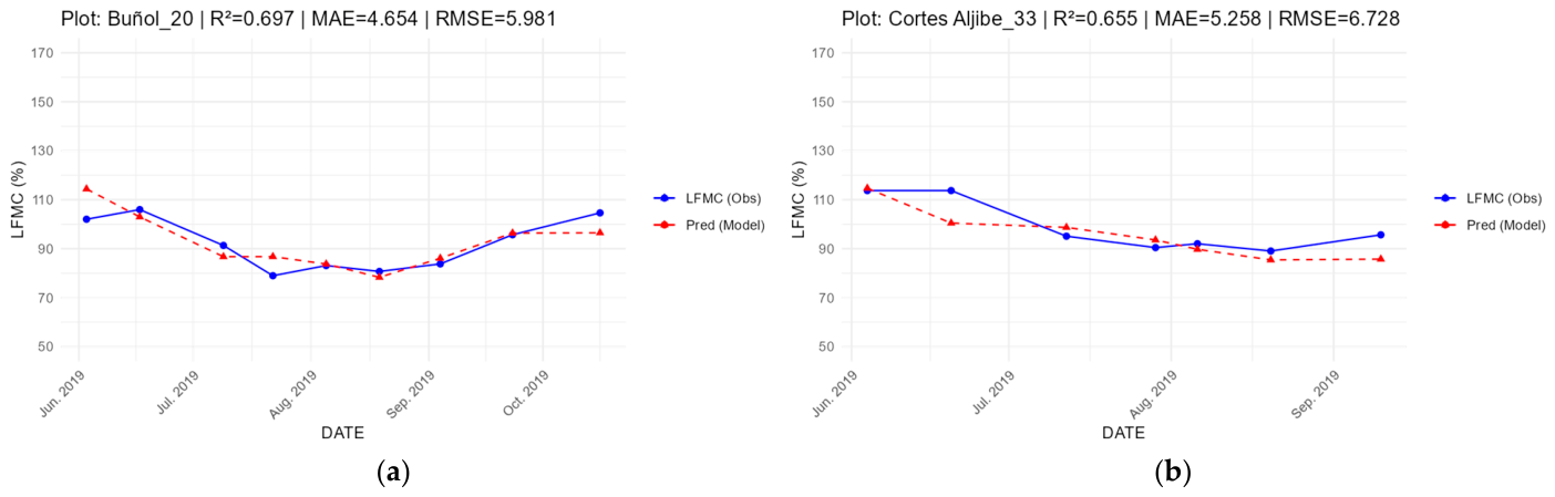
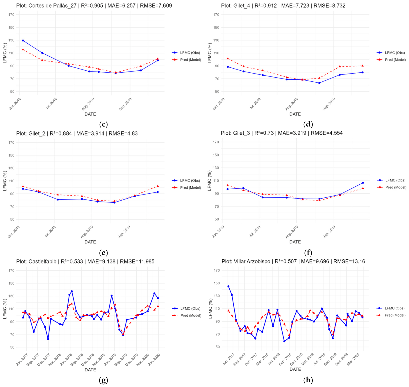
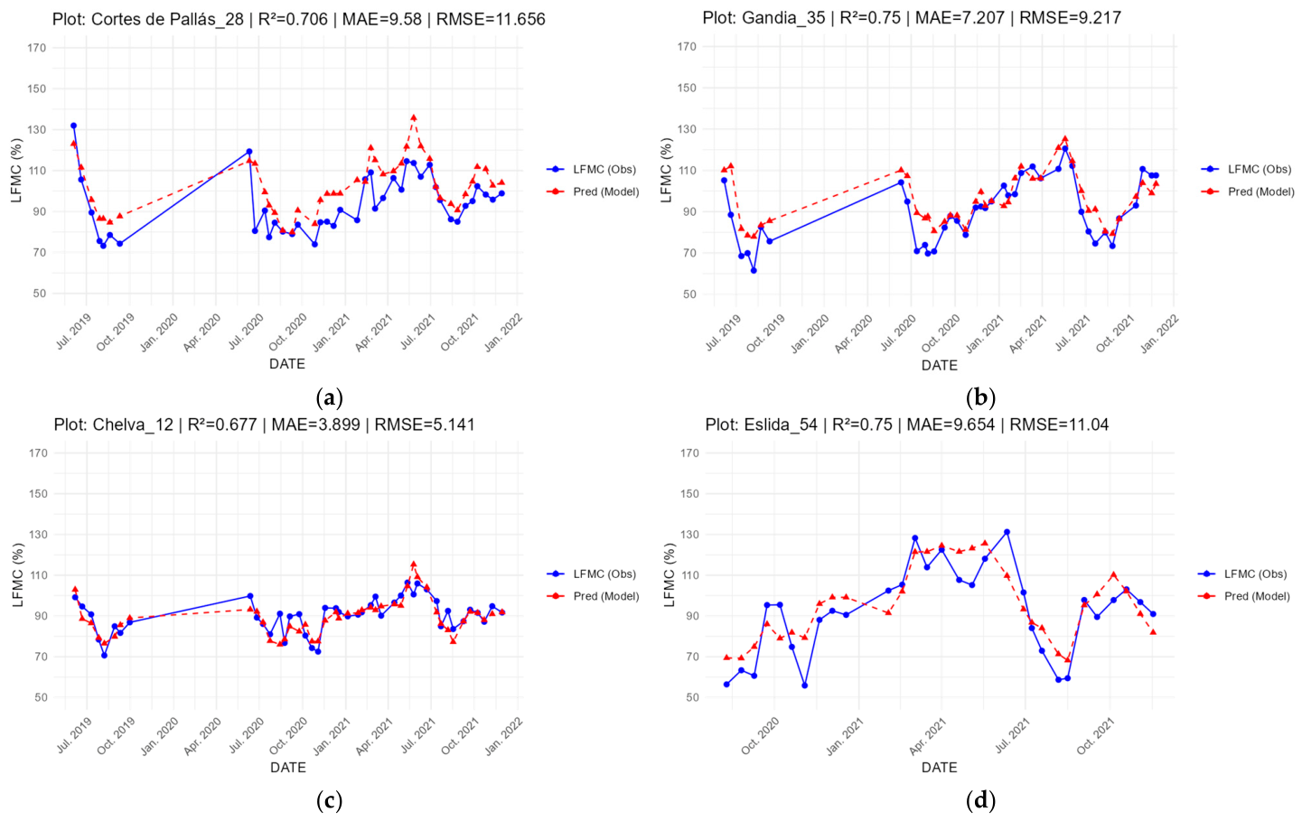
Figure 3 shows the temporal evolution of the observed and predicted values of the weighted average LFMC for selected plots under the A1 validation scenario. Some of the selected plots are located in close spatial proximity, providing illustrative examples of model predictions at neighbouring sites. For example, the distance between the Cortes de Pallás_27 and Cortes Aljibe_33 plots is approximately 4.2 km, while the three plots located in Gilet (Gilet 2, Gilet 3, and Gilet 4) are separated by distances ranging from 235 m to 725 m. The reported distances simply describe the spatial relationships among the illustrative examples presented in Figure 3 and are independent of the adopted validation strategy. The results show that the model reproduces the main temporal patterns of LFMC across these selected validation plots.

It is important to note that spatial proximity between validation plots does not necessarily imply ecological similarity. For example, although Gilet 2 and Gilet 3 are located only a few hundred metres apart, they differ markedly in vegetation composition, species fractional canopy cover (FCC), and fuel structure. Gilet 2 is characterised by a very dense shrub layer with high horizontal and vertical continuity, whereas Gilet 3 is characterised by woody shrubs with a continuous shrub-litter layer. In addition, the dominant species differ substantially, with Pinus halepensis representing approximately 35% of the FCC in Gilet 2 compared with about 70% in Gilet 3, while Erica multiflora accounts for around 20% and 3% of the FCC, respectively. The two plots also differ in the presence of other shrub species, such as Quercus coccifera and Phillyrea angustifolia. Consequently, despite experiencing similar regional meteorological conditions, these plots represent distinct vegetation configurations, which may lead to different LFMC responses.

In addition, differences in model performance were quantified among validation plots within Scenario A (validation period 2017–2020). The average RMSE was notably lower for plots with observations exclusively in 2019 (mean RMSE = 9.09), compared to the remaining plots with observations across multiple years within the 2017–2020 period (mean RMSE = 12.11). The observed variability is likely associated with interannual differences in meteorological conditions, particularly in precipitation patterns, as illustrated in the ombrothermic diagram (Figure S4, Supplementary Materials), which shows marked contrasts in rainfall distribution among years. These results help contextualise the patterns shown in Figure 3.

3.1.2. Validation A2: Testing on Later-Period Data (2022–2025)

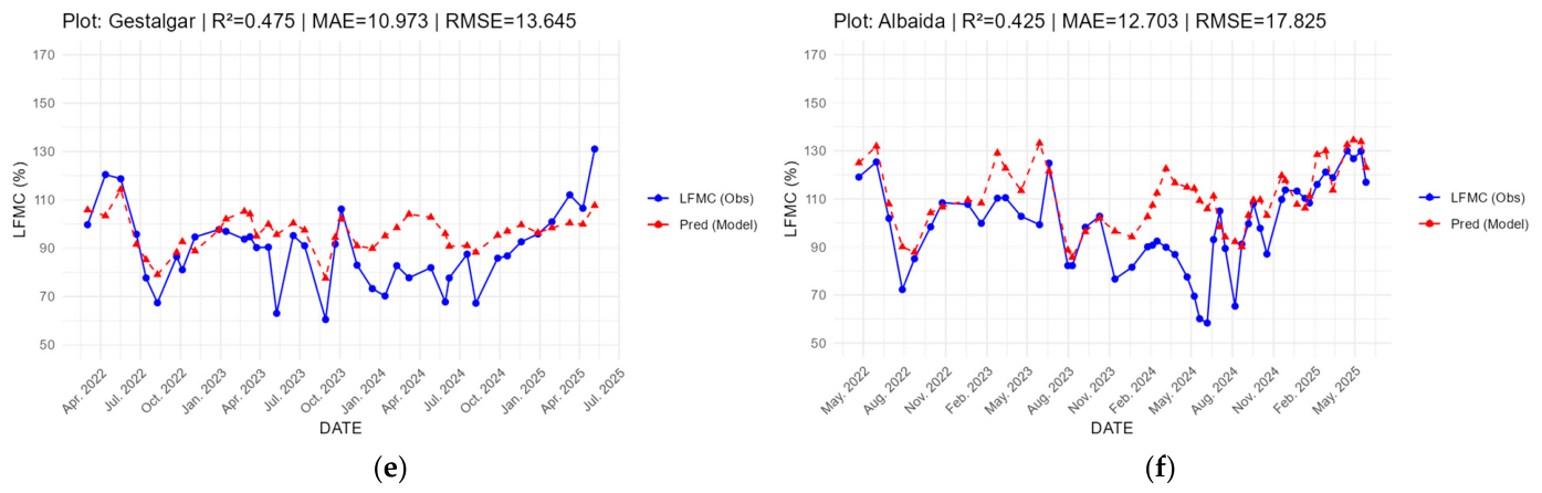
The second validation subset included samples collected between January 2022 and June 2025. In this case, the model performed worse compared to Validation A1, with larger errors and lower coefficients of determination. In contrast to the previous case, for validation during the 2022–2025 period, 10 out of 30 plots used for testing differed from the training set.

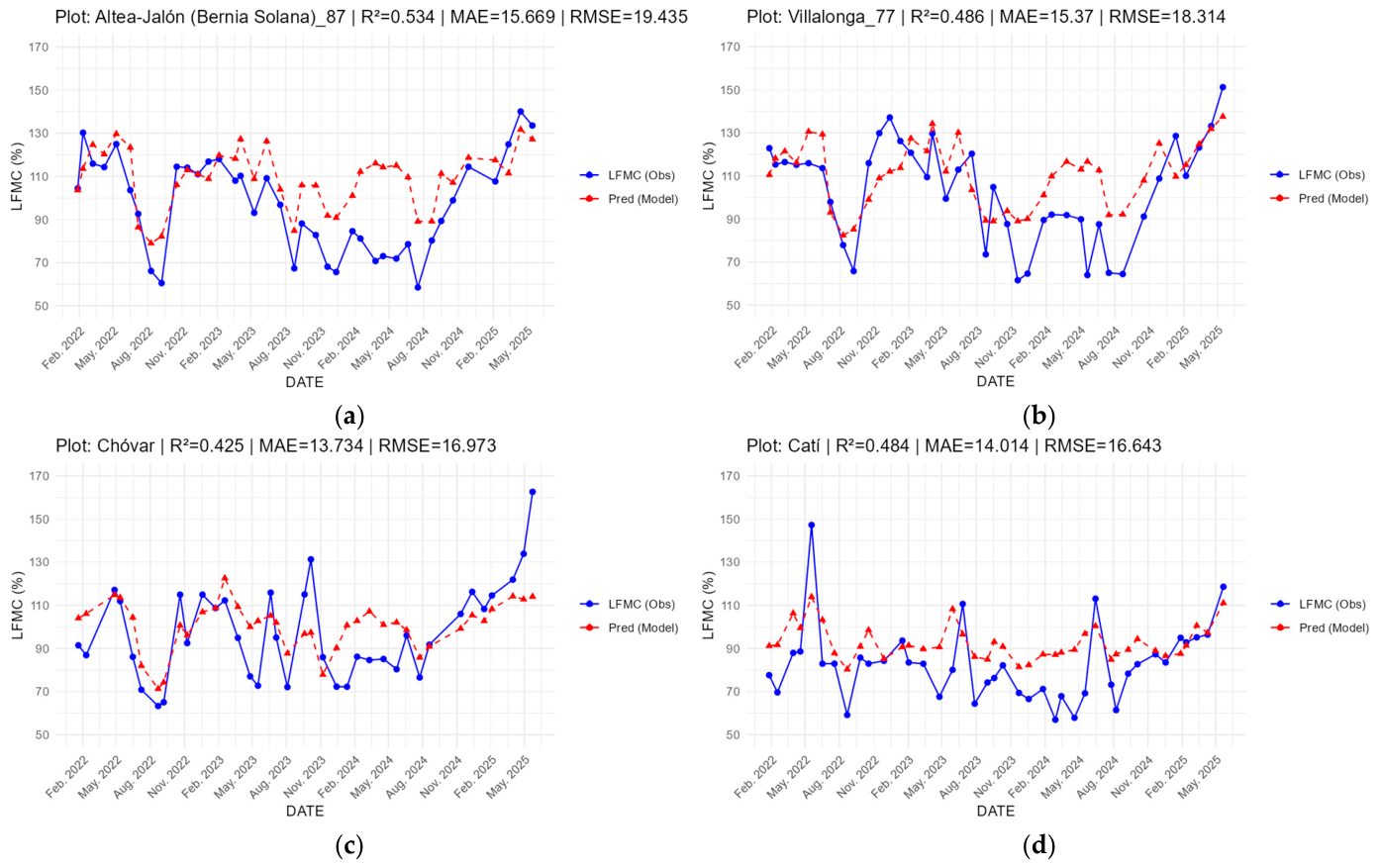
As shown in Figure 4, predictions tended to differ more strongly from observed LFMC values, particularly during periods characterised by higher summer temperatures and altered precipitation patterns (Figure S5). However, the model reproduced more accurately the dates closest to the end of the training period (around 2021), indicating better performance under conditions similar to those represented in the calibration dataset. A good agreement is also observed during the wetter period, spanning from October 2024 to 2025, even in plots such as Catí, which exhibit a relatively low variability in predicted values. In contrast, the model shows greater difficulty in capturing the lowest LFMC values, which are associated with the driest conditions and are particularly relevant from a fire-risk perspective.

To evaluate whether model performance differed between plots included in the training phase and the new ones, RMSE values were compared between both groups for the A2 validation period (2022–2025). The average RMSE obtained for plots that had been used during model training was 18.31, with a standard deviation of 7.74, while a very similar mean RMSE of 18.19 was observed for plots not included in the training dataset, with a lower standard deviation of 3.98. Although variability was higher for training plots, this was driven by a small number of sites exhibiting markedly higher prediction errors, in several cases associated with a limited number of available LFMC observations. Overall, the comparable mean RMSE values indicate that model performance during post-training validation was not systematically affected by whether a plot had been previously included in the training phase.

3.2. Scenario B: Spatial Generalisation with Training Data from 2017 to 2025

Results in Scenario B indicate that the model achieved consistent performance across validation sites, demonstrating its capacity to generalise spatially when trained on a temporally comprehensive dataset (see

Table 2. Model performance metrics for Scenario B (training: 2017–2025; spatially independent validation).

Dataset	No. Samples	R2 Adj (%)	RMSE	MAE
No. training plots: 54	3171	56.688	13.446	10.775
No. testing plots: 13	602	57.836	11.469	9.447

and Figure 5). Although the coefficient of determination was slightly lower compared to Scenario A within the training period, prediction errors remained within acceptable ranges, and overall stability improved. It should be noted that the training dataset in Scenario B comprised 3171 samples (Table 2), approximately 1.9 times the number of samples used in Scenario A (1670 samples; Table 1).

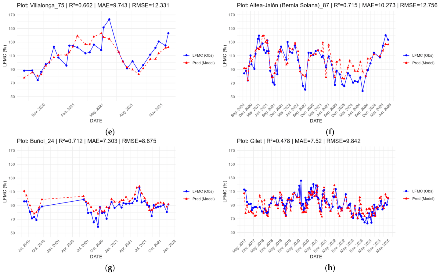
As shown in Figure 5, model predictions exhibit good agreement with observed LFMC values during the testing period. The interval between June 2019 and December 2021 corresponds to the period with the highest availability of field observations across the study plots, which explains why a larger number of plots were selected for model testing within this interval.

The temporal patterns illustrated in Figure 5 reveal plot-specific differences in model performance that can be related to the spatial proximity and temporal coverage of the training data. For the Gilet plot, several nearby plots (Gilet 2 and Gilet 3) were included in the training dataset, providing spatially close reference information. However, field observations for these neighbouring training plots are limited to the period between 2019 and 2021. This restricted temporal coverage likely contributes to the lower predictive performance observed for the Gilet plot during earlier years (2017–2018) and again after 2023, when model predictions extend beyond the temporal range represented in the training data.

A comparable situation is observed for the Altea-Jalón (Bernia Solana)_87 plot. In this case, the closest plots used for training are Xaló_86 and Xaló_88, both of which provide field observations only from September 2020 to November 2021. Between September 2023 and September 2024, observed LFMC values at Altea-Jalón (Bernia Solana)_87 are notably lower than those recorded during previous winter and spring periods, representing conditions that differ from those captured in the neighbouring training plots. As a result, predictions during this interval show increased deviations from the observed values, reflecting the temporal distance between validation conditions and the available training data.

Differences in the predictive behaviour for Altea-Jalón (Bernia Solana)_87 can also be identified by comparing its results in Figure 4 and Figure 5. While prediction errors increase for the September 2023 to September 2024 period under Scenario A, the corresponding results under Scenario B show improved agreement with observed LFMC values over the same interval. This comparison suggests that incorporating more recent field observations into the training dataset enhances model performance when predicting LFMC under temporally evolving conditions.

Additionally, the overestimation of LFMC observed for the Buñol_24 plot can be partly explained by differences in vegetation composition relative to nearby plots used for model training (Buñol, Buñol_20, Buñol_21, and Buñol_semanal). Buñol_24 is characterised by a markedly higher FCC of Quercus coccifera (50%) and Juniperus oxycedrus (30%) compared with the neighbouring training plots, which exhibit a greater relative contribution of more xerophytic shrub species such as Ulex parviflorus, or Cistus albidus. Furthermore, given that the LFMC response variable is computed as a weighted average by species fractional canopy cover, the dominance of species typically associated with higher and more stable moisture content leads the model to predict higher LFMC values. When combined with local conditions yielding lower observed LFMC (Buñol_24), this compositional difference results in systematic overestimation, reflecting a degree of extrapolation beyond the vegetation structures represented in the training dataset.

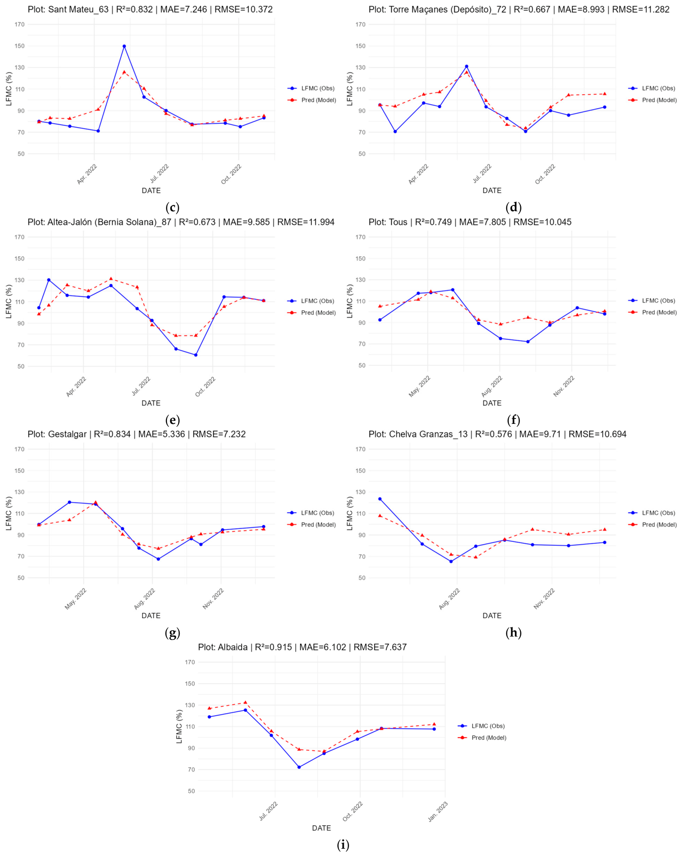
3.3. Scenario C: Year-by-Year Temporal Generalisation

3.3.1. Training 2017–2021, Testing 2022

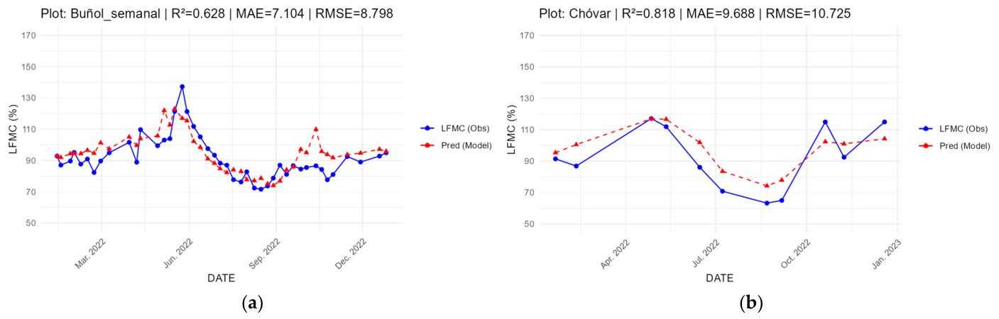
As shown in

Table 3. Model performance metrics for Scenario C (training: 2017–2021; testing: 2022).

Year	No. Samples	R2 Adj (%)	RMSE	MAE
Training: 2017–2021	2376	56.919	12.555	10.172
Testing: 2022	371	65.512	12.849	10.837

and Figure 6, when trained on data from 2017 to 2021 and evaluated on samples from 2022, the model showed satisfactory predictive performance, with metrics remaining within expected ranges.

It is worth highlighting that, for the plot referred to as Buñol_semanal, field observations were collected at a weekly interval (every 7 days), in contrast to the monthly sampling frequency applied in most other plots. The temporal behaviour of the Buñol_semanal plot was consistent with that observed in the other plots shown in Figure 6, although represented by a higher number of observation dates.

With regard to Figure 6, model predictions successfully reproduce the pronounced increase in LFMC observed during spring 2022, following several months characterised by higher-than-usual precipitation. The predicted trajectories also capture the sharp decline in LFMC during the summer and early autumn months, which is partly associated with above-average temperatures during this period. These temporal patterns are consistent with the climatic conditions reported by the Spanish Meteorological Agency (AEMET) in its monthly climatological summary reports, which document anomalously wet conditions during spring 2022, followed by unusually warm and dry conditions in summer and early autumn (AEMET climatological summaries; https://www.aemet.es/es/serviciosclimaticos/vigilancia_clima/resumenes?w; last accessed: 13 January 2026). To further contextualise these observations, the ombrothermic diagrams presented in the Supplementary Material (Figures S4 and S5) display average temperature and accumulated precipitation not only for the study period but also relative to the historical climatological baseline for 1981–2010, providing a reference framework for identifying the climatic anomalies influencing LFMC dynamics during the validation year.

3.3.2. Training 2017–2022, Testing 2023

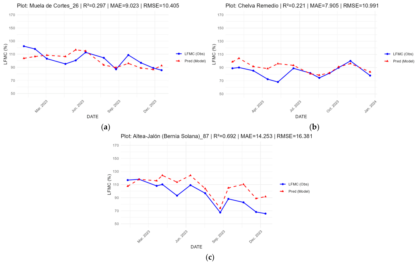
When extending the training dataset to include 2022 and testing on 2023 samples, model performance decreased substantially. Metrics, shown in

Table 4. Model performance metrics for Scenario C (training: 2017–2022; testing: 2023).

Year	No. Samples	R2 Adj (%)	RMSE	MAE
Training: 2017–2022	2748	60.611	12.567	10.179
Testing: 2023	435	22.109	15.570	12.720

, indicated weaker agreement between predicted and observed LFMC values.

This behaviour can also be observed in Figure 7:

As illustrated in Figure 7, the predictions for 2023 reflect a markedly different spring behaviour compared with the previous year. According to records from the Spanish Meteorological Agency (AEMET), March 2023 was the second warmest on record (only surpassed by March 2001) and the driest since records began, while April 2023 was also the second warmest (only exceeded by April 2014), the driest, and the sunniest April on record. For two consecutive months during the spring of 2023, climatic conditions were classified as very warm and extremely dry. These anomalous conditions are reflected in the field observations, which show unusually low LFMC values during spring 2023, in sharp contrast with the wetter spring observed in 2022.

Although the model accounts for previous cumulative precipitation including ln(1 + p60) as an independent variable, LFMC predictions are also influenced by static predictors such as the sine and cosine of the day of year, whose contribution within the Random Forest framework may depend more strongly on the temporal characteristics represented in the training dataset. This dependence contributes to reduced sensitivity to atypical spring conditions when those deviate substantially from those observed during the training period.

This effect is particularly evident for the Altea-Jalón (Bernia Solana)_87 plot when comparing predictions for 2022 (Figure 6) and 2023 (Figure 7). While observed LFMC values during summer are lower in 2023 than in 2022, model predictions for 2023 remain closer to those obtained for the previous year. Despite this, the model is still able to reproduce the overall seasonal dynamics, capturing the general decline during summer and early autumn, albeit with reduced accuracy under the exceptionally dry and warm conditions experienced in 2023.

3.3.3. Training 2017–2023, Testing 2024

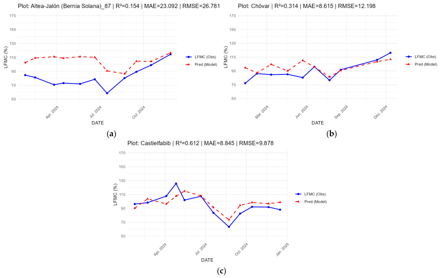
Using samples from 2017 to 2023 for training and testing on 2024 data resulted in mixed performance. While some metrics showed slight improvement compared to the previous case (Training 2017–2022, testing 2023), others remained similar or worse, and overall predictive capacity remained limited, as shown in

Table 5. Model performance metrics for Scenario C (training: 2017–2023; testing: 2024).

Year	No. Samples	R2 Adj (%)	RMSE	MAE
Training: 2017–2023	3183	58.606	12.576	10.128
Testing: 2024	422	21.630	17.695	15.286

.

Figure 8 shows that LFMC predictions for 2024 exhibit reduced agreement with field observations at several sites, particularly during the winter and spring periods. This behaviour is exemplified by the Altea-Jalón (Bernia Solana)_87 plot, where predicted LFMC values deviate more markedly from observations during early 2024. Similar patterns are observed across most of the analysed plots, indicating a generalised decrease in predictive accuracy during this period.

Winter and spring 2024 were persistently characterised by low precipitation, following the dry conditions already recorded during the final months of 2023 (See the ombrothermic diagrams in the Supplementary Material, Figures S4 and S5). These antecedent dry conditions likely contributed to unusually low observed LFMC values, particularly during seasons when higher moisture levels are typically expected. Under these circumstances, model predictions exhibit greater discrepancies, reflecting the difficulty of extrapolating LFMC under prolonged and atypical dry conditions that extend beyond the range of variability represented in the training data.

From all plots analyzed, only one—shown in Figure 8c—exhibited metrics consistent with the model design.

In summary, in Scenario C, the model trained on data from 2017 to 2021 achieved satisfactory performance when predicting LFMC in 2022, indicating that model generalisation remained effective when validation meteorological conditions were still broadly consistent with the historical range captured during training. In contrast, predictive accuracy decreased markedly when extrapolating to 2023 and 2024, even when the training dataset was progressively extended to include data from 2022 and 2023. This decline reflects a reduced ability of the model to reproduce LFMC patterns under subsequent years characterised by altered meteorological conditions and changing temporal dynamics.

3.4. Comparative Summary of Scenarios

Across the three scenarios, Random Forest models showed good performance when applied within the temporal domain represented in the training dataset and reasonable spatial generalisation to plots not used for training. Overall, these results highlight clear behaviour differences between spatial and temporal extrapolation and show that, while Random Forest models can be spatially and temporally extrapolated in the short term, their predictive performance decreases as the differences from the original training conditions increase. These patterns are further illustrated in the figures provided in the Supplementary Materials (Figures S1–S3), which show the temporal evolution of observed and predicted LFMC values at three plots where field observations are available since 2022. These plots are far from those used for training up to 2021 and were selected to enable a more detailed assessment of model performance under combined spatial and temporal extrapolation across scenarios.

At the Albaida plot, the largest prediction errors occur between January and September 2024, a period during which observed LFMC values are consistently lower than those recorded during the same months in previous years. Incorporating data from the full training period (2017–2025) reduces prediction errors during this interval, even when the additional training data comes from other plots within the study region, highlighting the benefits of expanding the temporal coverage of the training dataset.

For the Yátova plot, the models are unable to reproduce the LFMC peaks associated with periods of high precipitation, such as spring 2022, autumn 2024, and March 2025. Nevertheless, extending the training dataset to include plots with observations from 2022 onwards improves model performance during dry periods, which are particularly relevant from a wildfire danger perspective.

In the case of Ares del Maestrat, the largest discrepancies between predicted and observed LFMC values occur during 2023. Model performance is notably reduced during dry periods when LFMC values fall below 70, indicating increased difficulty in reproducing extreme low-moisture conditions under combined spatial and temporal extrapolation. This behaviour is consistent with the vegetation composition of the plot, where Rosmarinus officinalis and Ulex parviflorus are the dominant species due to their high fraction of canopy cover (FCC). Among all species present, these two are typically the first to be affected under warm and dry climatic conditions, such as those recorded throughout 2023, which is reflected in low LFMC values and, consequently, in a reduction in the plot-level weighted average LFMC.

3.5. Comparative Spatial Validation (Summer 2021 and 2022)

To evaluate the operational performance of the Random Forest models under real mapping conditions, an independent spatial validation was conducted for two representative summer dates: 14 July 2021 and 8 August 2022. These dates were selected to represent contrasting seasonal conditions, ranging from relatively moderate summer moisture levels to more pronounced drought conditions. For each date, spatial LFMC predictions were generated using the two modelling approaches considered in this study (Scenario A and Scenario B) and the Random Forest model presented in [31]. Model performance was assessed by comparing predicted LFMC values with field observations available for plots sampled close to each corresponding date. In addition to the spatial prediction maps, prediction error distributions and BIAS metrics were analysed to evaluate the consistency and robustness of the models under operational conditions.

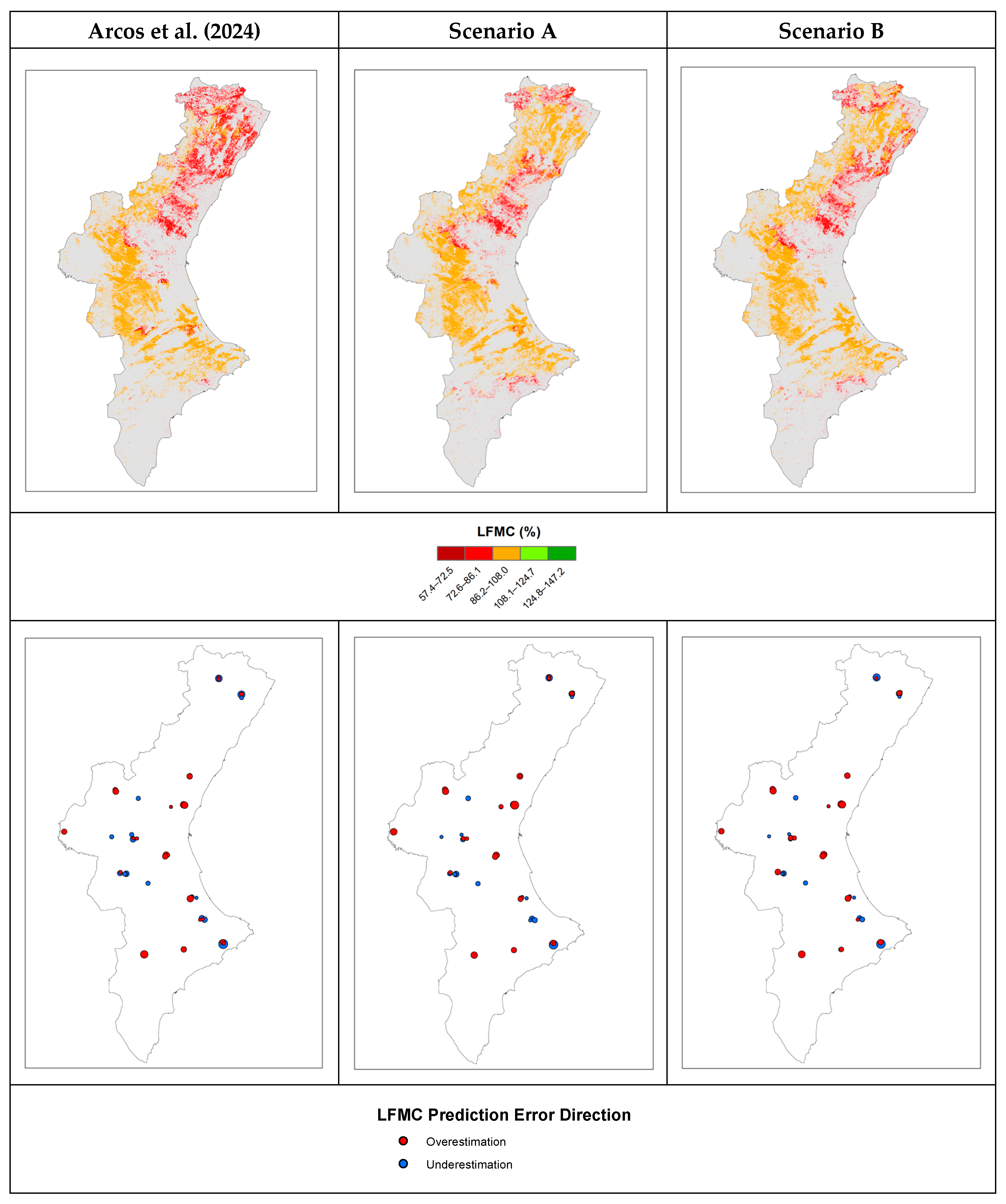
3.5.1. July 2021

For 14 July 2021, differences were distributed around zero across the three models. Most absolute errors remained within the range defined by the respective structural RMSE values. No systematic overestimation or underestimation pattern was observed. This behaviour is also reflected in the bias (BIAS) values calculated for the three models. Bias remained very close to zero, with values of +0.99% for Scenario A, +0.87% for Scenario B, and −0.34% for the model presented in [31]. These values confirm that cartographic LFMC estimates were well centred for this date, with only negligible systematic deviation. This pattern is consistent with the prediction error maps shown in Figure 9 (lower panel), where positive and negative differences between predicted and field LFMC values are distributed around zero across the study plots.

In July 2021, all plots shown in Figure 9 (lower panel) were used for training the model in Scenario A; however, field measurements were not available exactly on 14 July in all cases, and comparisons were therefore based on observations from nearby dates. In contrast, in Scenario B, 13 plots were not used for training because they were part of the testing phase; however, the prediction errors observed at these plots did not increase significantly. Similarly, for the model developed in [31], 16 of these plots were not included during the training phase; among them, only three exhibited RMSE values higher than expected according to the model design, while the remaining plots did not show a substantial increase in prediction error. Overall, the model presented in [31] displayed a comparable dispersion of errors, although isolated deviations exceeding ±17.5 were observed in specific plots.

Figure 9 (upper panel) shows a consistent spatial pattern across the three Random Forest implementations. Taken together, cartographic performance for July 2021 was consistent with the internal validation metrics of each model. Lower LFMC values are predominantly distributed in the northern and interior mountainous areas of the region, while intermediate values appear more frequently in southern and coastal zones. Scenario A and Scenario B display very similar spatial structures, with only minor differences in the extent of intermediate LFMC classes. The model presented in [31] exhibits slightly greater spatial contrast in some northern areas, with a somewhat broader representation of the lowest LFMC class. However, general dry–wet transitions are coherent across all three maps.

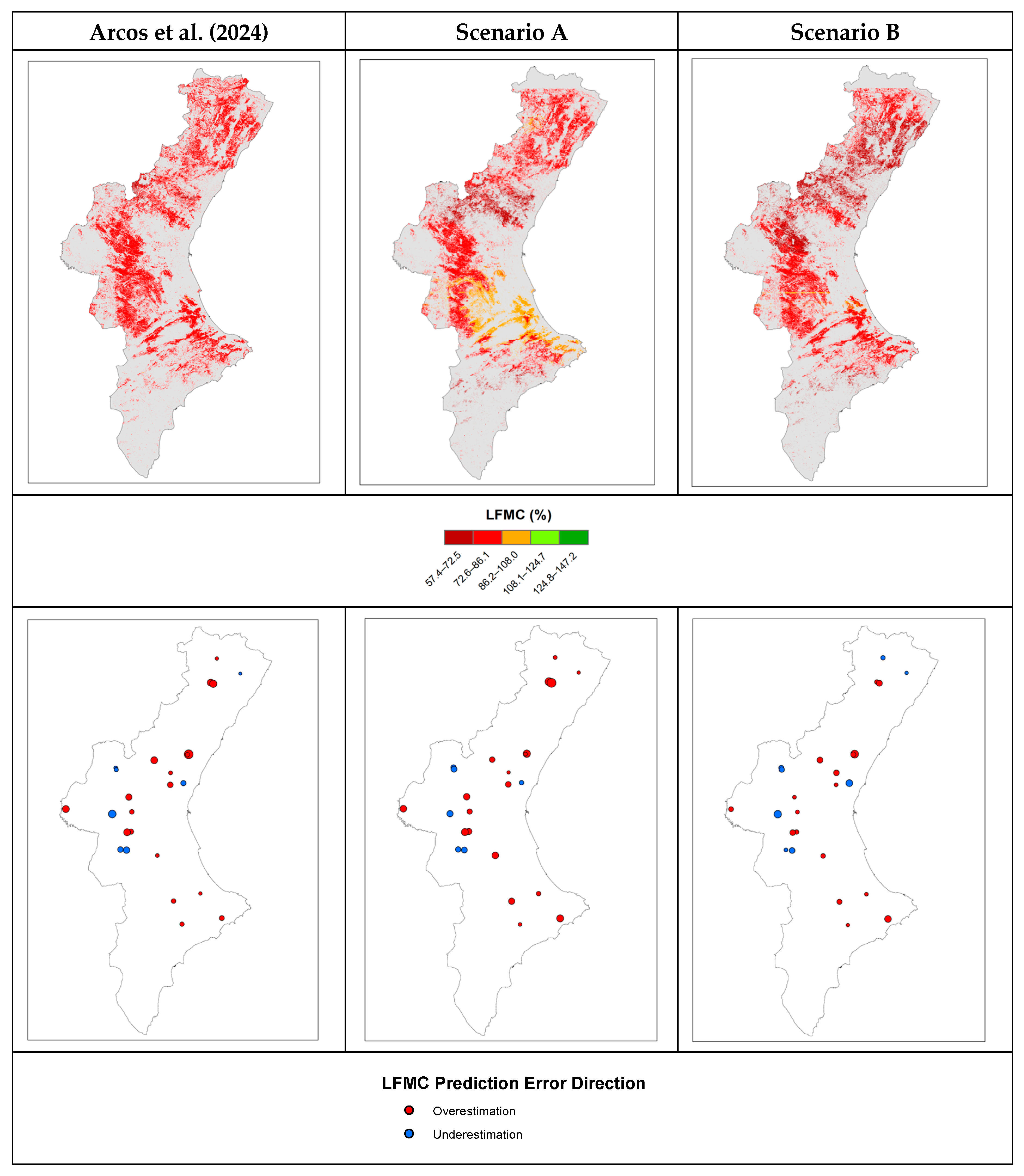
3.5.2. August 2022

For 8 August 2022, a different pattern emerged. Differences were predominantly negative across the three models, indicating a tendency to overestimate LFMC under dry summer conditions. The BIAS analysis confirms this systematic tendency. Bias values increased substantially compared with July 2021, reaching +5.63% for Scenario A, +2.32% for Scenario B, and +4.66% for the model presented in [31]. These results indicate a consistent overestimation of LFMC across all models under the drier conditions of summer 2022, with Scenario B showing the lowest systematic deviation. This tendency is also visible in the prediction error maps shown in Figure 10 (lower panel), where positive differences (in red) between predicted and field LFMC values predominate across the sampled plots.

Several plots exhibited absolute errors exceeding the structural RMSE values derived from the training datasets (Table 1 and Table 2), particularly in sites with low observed LFMC. Scenario A showed the largest deviations in these cases. Scenario B reduced the magnitude of the error in multiple dry plots (e.g., Ares del Maestrat, Catí, Tous, Yátova), while the model described in [31] also exhibited overestimation under these conditions. Across models, larger deviations were observed when LFMC values were low. Although minor temporal offsets existed between field measurements and cartographic dates, the overall error pattern remained consistent across plots.

In contrast to the July 2021 mapping, several plots shown in Figure 10 (lower panel) were not used during the training phase of the models. In Scenario A, nine of the plots represented in Figure 10 were not included in the training dataset, three of which exhibited prediction errors ranging between 15% and 23.5%. Similarly, for the model developed in [31], 17 plots were not part of the training phase, among which seven showed errors ranging between 15% and 23%. By comparison, Scenario B included a larger proportion of these plots within its training dataset, with only two plots excluded from training; in these cases, the observed prediction errors remained slightly below 15.

For 8 August 2022 (Figure 10, upper panel), the cartographic patterns differ markedly from those observed in 2021. Low LFMC values dominate most shrubland areas across the region, indicating widespread dry conditions. Although the three models reproduce this generalised drying pattern, noticeable differences emerge. Scenario A shows localised areas classified within intermediate LFMC ranges, particularly in central and southern sectors, suggesting partial smoothing of extreme dryness. In contrast, Scenario B presents a more extensive representation of the lowest LFMC classes in these areas, reducing the spatial extent of intermediate values. The Random Forest model from [31] also depicts widespread low LFMC values, though with some differences in spatial continuity compared to Scenarios A and B. These visual differences align with the plot-level evaluation, where August 2022 was characterised by predominantly negative differences (field − predicted), indicating systematic overestimation of LFMC under dry conditions, but with errors remaining below 23.5 in all comparisons with field observations from nearby dates.

4. Discussion

4.1. Temporal Extrapolation Under Changing Environmental Conditions

The results show that models trained to estimate live fuel moisture content (LFMC) exhibit strong limitations when extrapolated beyond the temporal domain represented in the training dataset. In Scenario A, models calibrated using data from 2020 to 2021 performed reasonably well when applied to earlier observations (2017–2020), but showed a marked decline in performance when evaluated on later periods (2022–2025). Similarly, Scenario C revealed that models trained on pre-2022 data could predict LFMC in 2022 with acceptable accuracy, whereas predictive skill deteriorated substantially for subsequent years.

These findings highlight the sensitivity of empirical and machine learning LFMC models to changes in precipitation regimes, temperature patterns, and seasonal water availability. When such shifts occur, models trained under earlier conditions may no longer capture the dominant controls on vegetation moisture dynamics, leading to degraded performance when extrapolated in time.

In this context, the limitation observed in temporal extrapolation is consistent with findings in other environmental machine learning applications, where models often maintain good performance under spatial or randomly split validation schemes but show substantial performance degradation when evaluated using temporally independent validation years [47]. This behaviour reflects the difficulty of reproducing patterns under conditions that fall outside the range represented in the training data, as documented in environmental modelling studies analysing extrapolation performance [48].

Consistent with this, the observed decline in model performance after 2021 coincides with documented changes in regional meteorological conditions, including higher temperatures and altered precipitation patterns. These shifts provide a plausible explanation for the reduced predictive skill, as they represent conditions that were not fully captured within the training dataset. The final predictor configuration combines seasonal descriptors (DOY sine and cosine) with year-specific meteorological variables (T60 and ln(1 + p60)), allowing the model to reproduce the general seasonal evolution of LFMC while accounting for interannual climatic variability. However, under exceptionally warm and dry conditions that fall outside the range represented in the training dataset, the influence of the seasonal descriptors may contribute to smoothing the expected temporal behaviour, thereby reducing sensitivity to atypical LFMC responses. This interpretation is further supported by the particularly large prediction errors observed during 2023, when exceptionally warm and dry spring conditions, documented by AEMET, resulted in unusually low LFMC values that were poorly represented within the temporal range of the training dataset. This, in turn, is reflected in the reduced temporal transferability of LFMC models under changing climatic conditions. Accordingly, LFMC–predictor relationships do not appear to be temporally invariant, and model generalisation across years cannot be assumed, particularly in Mediterranean environments subject to increasing climatic variability. These findings reinforce the importance of continuously updating operational LFMC models with newly acquired field observations spanning a broader range of climatic conditions.

In addition, alongside temperature (T60) and precipitation (ln(1 + p60)), vapour pressure deficit (VPD) was also considered as a potential predictor, derived from meteorological station data. VPD has been widely used as an indicator of atmospheric moisture demand and vegetation water stress, and its relevance for LFMC estimation has been highlighted in studies such as Jolly et al. [49]. Based on this, VPD was evaluated during the selection process. Although it showed a level of importance comparable to that of T60, its inclusion neither significantly improved model performance nor provided sufficient explanatory gain to replace T60 in the final predictor set. Consequently, it was not retained in the adopted configuration. Similarly, the selection of TCARI as the only spectral predictor should not be interpreted as indicating that other spectral indices related to vegetation condition were uninformative. During the feature selection process, several spectral indices—including the water-sensitive indices NMDI, NDMI, and NDWI, as well as the vegetation indices Vgreen and VARI—also showed substantial predictive potential for LFMC estimation. These indices capture complementary aspects of vegetation condition, including canopy water content, vegetation vigour, physiological status, and photosynthetic activity, all of which are closely linked to LFMC dynamics. However, once seasonal and meteorological predictors were incorporated into the Random Forest model, the inclusion of these alternative spectral indices did not provide sufficient improvement in predictive performance to justify increasing model complexity. Therefore, following the principle of parsimony, TCARI was retained because it achieved comparable predictive performance while preserving methodological consistency with the Random Forest framework previously developed in [31]. Building upon this validated framework allowed the present study to specifically evaluate the effects of extending the methodology from a local to a regional scale and from a short-term to a multi-year operational framework, while incorporating the methodological refinements introduced in the present study.

4.2. Spatial and Temporal Generalisation in Operational LFMC Monitoring

A central finding of this study is the contrasting behaviour of Random Forest models with respect to spatial and temporal generalisation. When trained on a temporally comprehensive dataset spanning the full study period (2017–2025), the models demonstrated stable performance when applied to plots not included in the training phase. In contrast, model performance consistently deteriorated when predictions were extrapolated to future periods characterised by climatic conditions that were not fully represented in the training data. While spatial extrapolation within a given climatic regime appears feasible, temporal extrapolation across evolving climate–vegetation interactions introduces substantially greater uncertainty, underscoring the need to account for temporal representativeness when designing operational LFMC prediction frameworks.

The observed spatial generalisation should be interpreted in the context of the adopted validation framework. Although the LLOCV approach ensures independence at the plot level, it does not eliminate potential spatial autocorrelation among nearby plots. As a result, some degree of spatial dependence may have influenced the validation results, particularly where neighbouring plots share similar environmental conditions. Future studies may explore complementary validation strategies based on explicit spatial buffer distances to further assess model transferability under stricter spatial independence criteria.

From an operational perspective, these results emphasise the importance of continuous model updating. Comparisons between scenarios show that incorporating newly acquired field observations into the training dataset reduces performance degradation and improves model robustness. Rather than treating recalibration as a methodological limitation, periodic retraining should be regarded as an essential component of LFMC monitoring systems operating over extended time frames. Such dynamic frameworks allow models to remain aligned with current climatic and ecological conditions, enhancing their reliability for wildfire danger assessment, fuel monitoring, and decision-support applications.

At the implementation level, spatial resolution is a key consideration for LFMC monitoring systems. The models currently implemented within the operational platform of the Valencian Region (https://prevencionincendiosgva.es/HCVivo, last accessed: 16 July 2026) rely on the retrieval of spectral information and the interpolation of meteorological variables at a spatial resolution of 100 × 100 m to generate regional LFMC maps. This existing operational framework was leveraged in the present study to assess the applicability of Random Forest models at the same spatial resolution.

An additional operational advantage of the proposed Random Forest framework is that it employs a single predictor configuration across the entire Valencian Region. In contrast, the operational linear methodology requires dividing the study area into different bioclimatic zones and selecting different predictor combinations for each zone. Furthermore, some linear models incorporate predictors based on long-term temporal averages of spectral indices, which require updating as new observations become available and may alter the optimal predictor set during recalibration. Consequently, maintaining and updating the linear framework over extended periods under changing climatic conditions becomes operationally more complex. The proposed Random Forest framework avoids this regional differentiation while maintaining a consistent predictor structure, thereby simplifying operational implementation and future model updating.

4.3. Comparison with Other Random Forest-Based LFMC Modelling Approaches

Recent studies have demonstrated the potential of Random Forest (RF) models for operational or near-operational estimation of live fuel moisture content (LFMC), although reported performance varies substantially depending on sensor choice, training sample size, vegetation representation, and validation design. In Portugal, ref. [36] developed a near-real-time RF LFMC product based on a small predictor set (drought code, day-of-year, and satellite vegetation indices) and reported R² = 0.78 and RMSE = 12.82% for the validation dataset, using LFMC measurements aggregated at site level across 16 sampling sites and MODIS-based inputs. While these results demonstrate the potential of RF approaches for operational monitoring, the limited number of sampling sites and the use of spatially coarse inputs constrain direct comparison with regional-scale applications based on higher-resolution data.

Among other studies conducted in Mediterranean environments, ref. [29] evaluated LFMC retrieval for both tree and shrub species in Spain using Sentinel-2 data at 20 m spatial resolution and reported a baseline RF performance of R² = 0.55, MAE = 15.1%, and RMSE = 19.7%, improving to R² = 0.63 and MAE = 13.4% when ancillary and static information (e.g., vegetation cover) was incorporated; the authors also noted a limited added value of Sentinel-1 SAR data in their experiments. Compared with the present study, their approach was evaluated over shorter temporal windows (2016–2020) and did not explicitly assess spatial and temporal extrapolation under operational conditions, which limits direct comparison despite the use of similar optical data sources.

At broader spatial extents, ref. [32] mapped LFMC across the Mediterranean Basin using RF models combining MODIS spectral/thermal information and day-of-year, reporting overall RMSE values of 19.9% (calibration period) and 16.4% (temporal validation period), with generalisation errors commonly in the ~16–20% RMSE range depending on vegetation type and season. While these subcontinental products emphasise scalability, their coarser resolution and heterogeneous vegetation sampling conditions differ markedly from regional implementations based on higher-resolution inputs. Complementarily, ref. [30] reported an RF application driven by Sentinel-2 predictors and intensive field sampling at two sites (246 samples, April–October 2022) in Southern Portugal, achieving R² = 0.69 with RMSE = 6.47% for LFMC at those sites; this highlights the accuracy gains that can be obtained under geographically and temporally focused sampling designs, but also underscores potential limitations for transferability beyond the sampled conditions.

Similarly, ref. [50] reported strong RF performance for species-level moisture estimation in Andalusia (Spain), with R² > 0.89 and a maximum RF RMSE of 0.744 (in log-transformed LFMC units). This approach relied on species-specific parameterisation and localised training conditions. In contrast, the present study targets regional operability by modelling weighted average LFMC using a unified predictor set applied consistently across shrublands in the entire Valencian Region.

Against this background, the RF models developed in the present study—implemented at 100 × 100 m resolution using a consistent predictor set across the Valencian Region—achieved comparable performance to published RF approaches when evaluated under operationally motivated validation strategies. In line with the limitations discussed above, published evidence and our results (R² = 57.83, RMSE = 11.46%, and MAE = 9.44%) suggest that differences in reported accuracy across studies are often driven less by the RF algorithm itself than by the representativeness and size of the field dataset, the degree of temporal non-stationarity encountered during testing, and the spatial scale and resolution at which LFMC is defined and modelled.

4.4. Spatial Validation Under Anomalous Dry Summer Conditions

The independent spatial validation reveals a clear contrast between performance under conditions falling within the range of the training dataset (July 2021) and performance under drier, more anomalous conditions (August 2022). In July 2021, all three Random Forest implementations behaved consistently with their structural RMSE, confirming that model performance during mapping remains stable when climatic conditions fall within the range represented during calibration. In contrast, August 2022 showed systematic overestimation of LFMC, particularly under low-moisture conditions. This pattern suggests that the models encounter limitations when extrapolated to meteorological regimes characterised by more severe drought conditions than those predominating during training. This contrast is also reflected in the bias analysis. While bias remained close to zero in July 2021 for all models, indicating well-centred predictions, substantially higher positive bias values were observed in August 2022. This confirms that LFMC was systematically overestimated under the drier summer conditions, particularly for Scenario A and the model presented in [31], whereas Scenario B exhibited a smaller increase in bias.

Importantly, Scenario B demonstrated improved robustness relative to Scenario A. The inclusion of additional temporal variability in the training dataset reduced error magnitude in several of the driest plots. This supports the hypothesis that expanding temporal representativeness enhances model stability under evolving climatic conditions. The similar degradation observed in [31] indicates that the limitation is not algorithm-specific but rather related to the representation of extreme climatic states within the training dataset.

From an operational perspective, the tendency to overestimate LFMC during very dry conditions is particularly relevant, as minimum LFMC values correspond to periods of elevated wildfire danger. However, even under these conditions, prediction errors remained within moderate ranges in most cases. For example, in Scenario B on 8 August 2022, 22 out of 26 plots (85%) exhibited absolute errors below 11.5, while the remaining plots (15%) showed errors below 19, despite temporal offsets of up to 15 days between field measurements and the cartographic prediction date. Although model updating mitigates this effect, complete elimination of bias under extreme drought conditions remains challenging. These findings reinforce the need for continuous temporal updating of LFMC monitoring systems in Mediterranean shrublands, especially under increasingly variable climatic regimes.

Overall, the spatial comparison highlights the stability of all models under conditions falling within the range of the training dataset (July 2021) and their differentiated behaviour under more severe drought conditions (August 2022). While spatial patterns remained coherent across implementations, the extended training dataset used in Scenario B appears to reduce the smoothing of extreme dryness observed in Scenario A.

Importantly, these results confirm that differences between modelling scenarios become evident primarily under anomalously dry conditions (2022), reinforcing the importance of temporal representativeness in operational LFMC monitoring systems.

4.5. Implications for Future Research

The limitations identified in this study highlight the need for methodological developments capable of improving temporal extrapolation under changing climatic conditions. The reduced predictive performance observed during the anomalously warm and dry years analysed here should not be interpreted solely as a consequence of unprecedented climatic conditions, but also as a manifestation of the inherent limitations of empirical machine learning models when extrapolating beyond the range of environmental conditions represented in the training dataset. Because Random Forest models are fundamentally data-driven, they cannot reliably infer relationships under climatic regimes that were insufficiently represented during model calibration.

Future work should therefore explore hybrid modelling approaches that integrate empirical machine learning methods with process-based or physically informed models to improve temporal robustness. Additionally, investigating adaptive training strategies, such as incremental learning or climate-regime-specific models, may help mitigate the effects of non-stationarity by allowing models to better accommodate evolving climatic conditions. Expanding long-term LFMC field datasets to encompass a broader range of climatic variability will also remain essential for improving model resilience and supporting more reliable operational LFMC monitoring under future climate scenarios.

5. Conclusions

This study demonstrates the potential and limitations of Random Forest models for regional-scale monitoring of live fuel moisture content (LFMC) in Mediterranean shrublands when evaluated under operationally realistic conditions. By extending a previously validated methodology to a multi-year (2017–2025) and spatially extensive dataset encompassing 67 plots across the Valencian Region, this work provides a robust assessment of both spatial generalisation and temporal extrapolation capabilities.

Results show that Random Forest models can generalise effectively across space when trained on datasets that capture sufficient temporal variability, enabling stable LFMC estimation in plots without direct field observations. In contrast, predictive performance consistently deteriorates when models are extrapolated to future periods characterised by climatic conditions not fully represented during training, particularly under extreme warm and dry conditions or during anomalous meteorological events that alter vegetation behaviour over short time intervals.

Importantly, the results indicate that model performance can be substantially improved through periodic updating of the training dataset while maintaining the same set of predictor variables. Scenarios incorporating newly acquired field observations show enhanced robustness and reduced performance degradation, underscoring the necessity of dynamic, continuously updated modelling frameworks rather than static calibrations.

The study further demonstrates the feasibility of implementing Random Forest models using a consistent set of spectral and meteorological predictors across the entire region. When regularly updated, the proposed approach provides an operationally scalable framework based on a consistent predictor configuration across shrublands throughout the Valencian Region. Compared with the currently implemented linear methodology, which requires different predictor sets for different bioclimatic zones and periodic redefinition during model updating, the proposed framework simplifies operational implementation while providing robust predictive performance under the adopted validation framework. This operational simplicity enhances regional deployment and scalability for wildfire danger assessment. However, these results also emphasise that model reliability may be compromised under atypical climatic conditions, reinforcing the need for continuous monitoring and cautious interpretation of predictions during extreme or rapidly changing environmental scenarios.