Physics-Based Modelling of Pine Needle Surface Fires and a Single Douglas Fir Tree: Comparison with Experiments

Abstract

Wildland fires, including surface and crown fires, present significant challenges for ecosystems and forest management. Accurate fire modelling is crucial for risk assessment and mitigation strategies. The Fire Dynamics Simulator (FDS) v6.8.0, developed by the National Institute of Standards and Technology (NIST), is a physics-based model that simulates fire behaviour by incorporating advanced physics and chemistry. However, its reliability requires thorough validation. This study validates FDS 6.8.0’s performance in modelling both surface fires and single tree burning. Two separate simulation sets were conducted. For surface fires, pine needle fuel beds were used at a laboratory scale to examine fire behaviour on slopes of 0°, 10°, and 20°. The results were validated against experimental data. A burning Douglas fir tree was simulated, and the results were compared with experimental measurements. The surface fire simulations at 0° and 10° slopes showed strong agreement with experimental data. In single-tree burning, both experimental and simulated results exhibited similar trends, with a rapid increase to a peak mass-loss rate (MLR) followed by a gradual decline. Validating FDS 6.8.0 forms an essential first step toward supporting the investigation of complex wildland fire behaviour, such as surface-to-crown fire transition, canyon fire, and dynamic escalation, using the same FDS version.

1. Introduction

Wildfires represent among the most significant natural calamities globally, often resulting in property damage and human casualties. Accurately predicting wildfire behaviour is crucial for effective fire control and reducing associated losses. Forest fires are typically classified into three main types: surface fires, crown fires, and subsurface (or ground) fires. Surface fires primarily burn vegetation and combustible materials on or near the ground surface. These materials include loose needles, moss, lichen, herbaceous plants, shrubs, small trees, and young trees. The burning is mainly through flames. The spread of surface fires largely influences fire expansion through these surface fuels. Subsurface fires, in contrast, smoulder slowly beneath the ground in organic matter, such as peat, duff, or roots, often persisting for extended periods without visible flames and potentially reigniting surface fires [1]. Surface fires can increase in intensity to the point where they scorch or even destroy the forest canopy, which is a characteristic observed in crown fires [2]. Due to the significant impact of fire on our economy, society, and environment, substantial efforts have been dedicated to developing empirical fire spread models, such as those developed by Rothermel [3] and McArthur [4]. Fire spread models are widely used for predicting surface fire spread rate and intensity. Most of these models, based on empirical observations, consider factors like fuel moisture, wind speed, and slope to estimate fire spread rates and have been widely adopted for practical fire management across various jurisdictions. These empirical and mathematical models are crucial for tasks like evacuation planning, fire suppression management, and preparedness activities [5].

Empirical fire spread rate models, such as McArthur [4], Rothermel [6], the Canadian Forest Fire Danger Rating System [7], and Vesta’s models [8], were developed in the last century to aid fire management. More recently, spatially explicit analogue fire behaviour platforms like FARSITE [9], PHOENIX Rapid-fire [10] and SPARK [11] have been introduced to forecast fire spread faster than in real time. Land management agencies widely utilize these models for operational purposes. These models offer rapid fire spread predictions that can readily apply to situations at field and community scales. However, they may occasionally yield non-physical outcomes [12]. Additionally, these models cannot predict fire behaviour within the complex mixture of vegetation and structural fuels found in the wildland–urban interface (WUI), which is characterized as the zone where residential structures are either within or close to natural vegetation and represents the prime area of concern in terms of wildfire risk to human populations. This heightened risk arises from the adjacency of potentially combustible vegetation to inhabited areas.

Given these limitations, there is a growing need for models that can better capture the complex dynamics of wildland fire behaviour. Advanced physical-based models, often utilizing a multiphase approach, have become valuable tools for investigating the underlying processes driving various phenomena associated with wildland fires [13,14,15]. This technique has been extensively reviewed in the wildland fire modelling literature [16,17,18]. In several studies, these models have been rigorously evaluated against detailed experimental measurements (beyond just spread rate), as the models’ accuracy relies on their capacity to predict the fundamental physical processes that govern overall fire behaviour. These models have been compared with experimental data on the burning characteristics of individual vegetation species [19,20,21], ignition, and flame spread in simplified fuel beds (such as pine needles, excelsior, and wood sticks) at laboratory scales [22,23,24,25,26,27] and more complex fuel beds at field scales [28,29].

Examples of physical-based models for wildland fire simulations include the Fire Dynamics Simulator (FDS) and the Wildland–Urban Interface Fire Dynamics Simulator (WFDS). The WFDS was developed as a vegetative fuel and fire model by the U.S. Forest Service (USFS) on the foundation of the FDS developed by the National Institute of Standards and Technology (NIST). While the WFDS is no longer being developed, it helped to extend the capabilities of the newer versions of the FDS by incorporating vegetation as a fuel source to simulate wildland fire behaviour. It includes two thermal degradation sub-models, a ‘linear’ model and an ‘Arrhenius’ model, both of which address different aspects of the pyrolysis process necessary for modelling vegetation combustion [30,31,32]. The FDS is now a three-dimensional, fully physics-based wildland fire model, which enables detailed simulations of fire spread across various vegetative fuels, such as trees, grasslands, and scrublands [33].

In recent years, a range of studies have utilized physics-based models to investigate fire scenarios, including surface fires and single-tree burning. These models provide detailed insights into fire dynamics by simulating the physical and chemical processes involved, enabling researchers to understand better and predict fire behaviour under various conditions. For grassland fires, prior simulations using the WFDS (compatible with older FDS versions) have established key consensuses on fire propagation dynamics. Mell et al. [17] employed the WFDS (FDS version 4) to model fire spread through surface fuels on flat terrain, comparing results to experimental data from Australian grassfire studies and empirical relations. Moinuddin et al. [29] simulated grassland fires with the WFDS (FDS version 6), achieving grid convergence at 250 mm and revealing linear relationships between fire spread rate and wind speed, as well as transitions from boundary-layer to plume modes with increasing grass height. Innocent et al. [34] examined wind and slope effects under low-speed winds, finding exponential relationships for spread rate, pyrolysis width, and fire intensity with slope angle, consistent with experiments. Collectively, these grassland studies demonstrate that physics-based models can reliably capture surface fire behaviours like spread rates and plume dynamics under controlled conditions, with good alignment to empirical and experimental data.

For tree and pine fuel simulations, similar validations highlight capabilities but also limitations in model versions and fuel specificity. For tree fires, Mell et al. [19] conducted experiments and WFDS modelling (FDS V4) on ignited trees of varying heights without wind, comparing mass-loss rates (MLRs) and heat fluxes, and noted strong influences from moisture and bulk density on burning characteristics. Yang et al. [35] experimentally studied pine needle fuel beds (1.2 kg/m² load) on slopes from −30° to 10°, revealing non-linear spread rate responses to downslope and dominant flame radiation heating, supported by a two-dimensional energy balance model. Recent validations include Wadhwani et al. [21] (FDS 6.7.8 for merging fires, with 5–35% errors in spread rates vs. Ribeiro et al. [36] experiments), Gupta et al. [37] (FDS 6.9.1 for single pine tree HRR and MLR), and Mueller et al. [22] (FDS 6.7.9 for quiescent pine needle flame spread, showing alignment in heat flux and MLR using simple decomposition models). However, a persistent limiting factor is that these studies rely on older or inconsistent FDS versions, often focusing on grassland or isolated scenarios without integrating slope effects on pine needle fuels and single-tree (e.g., Douglas fir) burning under a unified, updated model—hindering reliable progression to complex wildland fire predictions. This study addresses this gap by validating FDS 6.8.0 against experimental data from Yang et al. [35] for pine needle surface fires on 0° and 10° slopes (focusing on ROS and flame length) and Mell et al. [19] for Douglas fir tree burning (focusing on MLR and heat flux), establishing benchmarks for advancing simulations of intricate behaviours like surface-to-crown transitions.

FDS version 4, released in 2004, employed more simplified treatments of combustion, radiation, and solid-phase pyrolysis, with limited coupling between gas-phase and solid-phase processes. In contrast, later releases introduced significant improvements in physical sub-models, numerical stability, and validation scope, making them more suitable for detailed fire behaviour and wildland fire simulations [38]. FDS 6.8.0 incorporates substantial advancements in pyrolysis, combustion, radiation, and near-wall flow modelling compared to previous versions. Its integrated pyrolysis–combustion framework, which couples a one-dimensional solid-phase model with a three-dimensional gas-phase representation, has undergone systematic validation against experimental data, demonstrating its reliability and accuracy [39]. Enhancements in radiation modelling refine heat transfer calculations for more precise thermal analysis. Additionally, the Lagrangian particle framework now supports heat transfer and pyrolysis for solid walls, improving the representation of particle behaviour in fire scenarios [40]. These improvements, along with enhanced numerical stability in multi-mesh computations, establish FDS 6.8.0 as a more robust tool for fire behaviour analysis. While FDS 6.9 and FDS 6.10 series are available, in terms of field-scale wildland fire modelling, their use does not change the predicted fire behaviour in any material way compared to FDS 6.8 unless one deliberately uses newer or experimental features introduced after version 6.8. The FDS 6.8 series is often considered the baseline, and results have been easier to reproduce historically. Before conducting any simulations with any version of the FDS, it is essential to validate that specific version against experimental data to ensure the model’s accuracy. For consistency for the investigation of complex wildland fire behaviour, such as surface-to-crown fire transition, canyon fire, dynamic escalation, vorticity-driven lateral spread, use of the same FDS version is desirable. Given the limited validation studies available for FDS v6.8, the novelty of this work lies in validating the model in relation to both surface fire and tree fire by comparing its simulation results with experimental data under similar fire conditions.

We selected two experimental studies for comparison: a surface fire in pine needles conducted by Yang et al. [35] and a single Douglas fir tree fire conducted by Mell et al. [19]. The experimental datasets used for validation in this study were obtained directly from these two references. In the surface fire simulations, we will evaluate the rate of spread (ROS) and flame length from our simulations against experimental measurements at slope inclinations of 0° and 10°. For the single Douglas fir tree simulation, we will compare our results for the mass-loss rate and heat flux for a 2 m tree with Mell’s experimental data. Mell et al. [19] used their experimental data in earlier work to validate the WFDS, which was based on FDS version 4. In the current study, the novelty lies in the validation of FDS 6.8.0, which is vastly different from FDS version 4. Recent efforts such as the FIRE-RES D5.4 report [41] have also applied FDS 6.8.0 to wildland fire scenarios, including Douglas fir tree burning, and included comparisons of mass-loss rate and heat flux with experimental data. However, the present study differs in its explicit disclosure of thermo-physical fuel properties, optimization procedures for kinetic parameters, and systematic grid-sensitivity analyses. In addition, this work integrates both pine needle surface fires and single-tree burning within a unified validation framework, providing a more comprehensive and reproducible reference for future FDS-based wildland fire simulations. Our simulations are configured to replicate conditions from the experimental setup, as described in Section 2. This validation process is designed to ensure that the simulation accurately represents real-world fire scenarios, thereby increasing confidence in the model’s predictive capabilities and its utility in understanding fire behaviour.

2. Methodology

In this study, the surface fuel consists of pine needles, and the simulated single tree is a 2 m high Douglas fir. For efficient parallel computing, the computational domain in the FDS is divided into subdomains and appropriate grid sizes in the near-field and far-field. It is to be noted that the FDS only uses structural (cuboid) mesh for a finite difference scheme. The FDS automatically calculates the time step size based on fulfilling the Courant–Friedrichs–Lewy condition (CFL) criteria.

Within the FDS, there are various turbulence sub-models: The LES (Large Eddy Simulation) sub-model integrates turbulence effects into the simulation by resolving large-scale motions while employing an eddy viscosity approach to model the effects of smaller-scale motions. The VLES (Very Large Eddy Simulation) sub-model is a modification of the LES that aims to only capture the largest turbulent scales using coarse filters. It provides a compromise between the computational efficiency of Reynolds-Averaged Navier–Stokes (RANS) models and the accuracy of the LES. The VLES is often used in situations where a balance between accuracy and computational cost is required. It is suitable for cases where the full resolution of the LES may be too computationally expensive, but more detail than RANS is still necessary. In our study, we will employ the VLES model (the default in FDS 6.8.0) for our simulation.

We have used Fuel Element (FE) model of the FDS, which is suitable for representing vegetation occupying specific volumes, such as trees. This model necessitates a gas-phase grid with adequate resolution to sufficiently depict temperature gradients and heat exchange between the gas and solid phases, as outlined in the FDS technical guide [32]. The FE model is required to resolve fuel elements such as needles, branches, etc.; therefore, for consistency, it was used in both scenarios: the surface fire and the single-tree fire. The Methodology Section of this paper is divided into two parts: the first details the approach used for surface fire simulations, and the second describes the methodology applied in simulating the single tree. It is important to note that the single-tree and surface fire simulations are conducted separately and are not interconnected. The results for each scenario are independently compared to the corresponding experimental studies to provide comprehensive validation across two distinct fire scenarios.

Part I: Simulation of Surface Fire

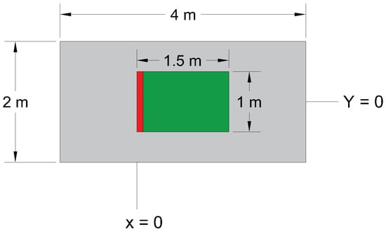
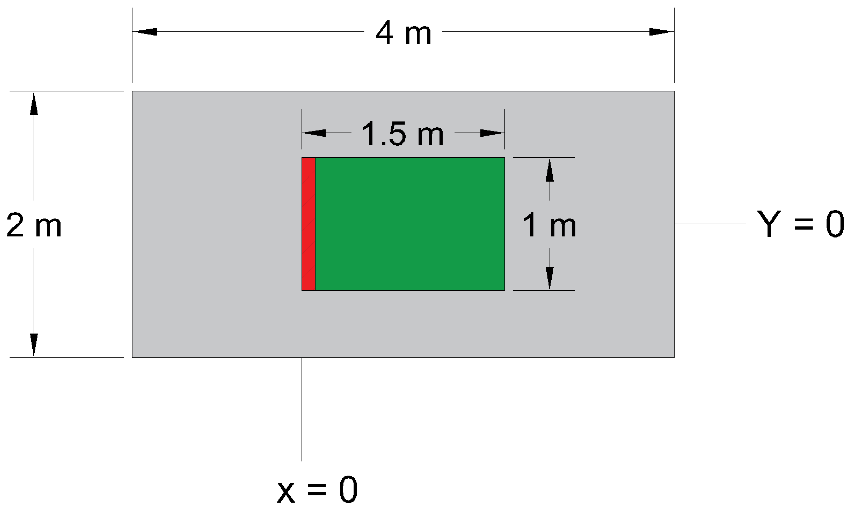
In this scenario, we followed the same setup used in the experimental work conducted by Yang et al. [35]. The domain length is 4 m from x = −1.25 to x = 2.75, the width is 2 m from y = −1 to y = 1, and the domain height is 2.5 m. The vegetative fuel bed in this scenario started from x = 0 to x = 1.5 m and from y = −0.5 to y = 0.5, so they are the same dimensions used in the experiment. Additionally, we followed the same experiment’s fuel load of 1.2 kg/m² in our simulations. The experimental study includes a range of slopes from −30° to +10°. For our simulations, we selected two cases from the experimental data—a zero slope and a +10° slope—and added a +20° slope case to examine the effect of increased slope on the rate of spread (ROS). It is to be noted that physics-based models have limitations in simulating fire propagation on downslopes [34]. Figure 1 shows the top view for the zero-slope case, and the red line represents the fire line. Table 1 shows a list of the thermo-physical and thermal properties utilized in this simulation. The properties assigned to the pine needle vegetation are based on Müller’s recent validation study using FDS version 6.7.9 [22]. Values for moisture content, relative humidity, and air temperature were taken from the experimental paper, varying from case to case, as shown in Table 1. To replicate real-world conditions, the inlet, outlet, sides, and top boundary were set as open, facilitating the inflow and outflow of air and matching with the real experiment.

Figure 1. The top view for the simulation.

Table 1. Thermo-physical, pyrolysis, and combustion parameters for the surface fuel.

Fuel Parameter	Values	Reference
Vegetative fuel	pine needles	[22]
Heat of combustion	17,700 kJ/kg
Surface area to volume ratio	4661 m−1
Moisture content	13.5% (zero slope) 11.6% (10° and 20° slopes)	[35]
Relative humidity	62% (zero slope) 59% (10° and 20° slopes)
Air temperature	8.9 °C (zero slope) 10.6 °C (10° and 20° slopes)
Fuel load	1.2 kg/m2
Ignition line intensity (HRRPUA)	150 kW/m2	Simulated condition
Thermal conductivity	100 W/m.K	[22]
Density	650 kg/m3
Pre-exponential factor A (dry vegetation)	1.18 × 103 s−1
Activation Energy E (dry vegetation)	6.58 × 104 J/mol
Pre-exponential factor $A$ (MOISTURE)	4.83 × 103 s−1
Activation Energy $E$ (MOISTURE)	3.91 × 104 J/mol
Pre-exponential factor $A_{char}$ (char oxidation)	465 m/s
Activation Energy $E_{char}$ (char oxidation)	68,000 J/mol

Two methods are available for simulating sloped terrain in the FDS. The common approach, known as the gravity method, involves adjusting the X and Z gravity components in the simulation input file to represent the slope, as described in the FDS user guide [40]. This method simulates the slope by effectively tilting the entire computational domain through modified gravitational forces, which primarily influence buoyant flow and create an uphill bias in plume tilt. However, because the underlying geometry remains flat, it often results in more uniform, two-dimensional flow patterns with limited lateral air entrainment from the sides of the fuel bed. Plume dynamics under this approach are driven by the altered buoyancy vector, leading to smoother plume rise angled along the effective slope but potentially underestimating turbulent mixing from surface irregularities. In terms of flame spread physics, the gravity method promotes faster uphill propagation due to the parallel gravity component assisting convective heat transfer, though it may not fully capture the intermittent flame attachment observed in real terrains [41].

The alternative, called the step method, creates a staircase of obstacles with a slope equal to the desired terrain angle. Utilizing the step method enhances air entrainment from the sides of the test bed into the flame, leading to more representative results compared to real-world scenarios. The stepped fuel arrangement facilitates airflow at varying angles, closely mimicking the complex entrainment dynamics observed in actual fire conditions [42]. Fundamentally, the step method introduces geometric discontinuities that generate vortical structures and increased turbulence, enhancing three-dimensional entrainment from gaps beneath and beside the steps. This results in more complex plume dynamics with greater mixing and variability, better replicating the asymmetric uphill/downhill flow patterns seen in experimental studies. For flame spread, the steps allow for localized preheating and flame attachment at edges, leading to more realistic spread rates that account for terrain roughness rather than assuming a smooth surface. The step method is thus more realistic beyond numerical agreement, as it physically approximates the irregularities and airflow pathways in natural sloped environments, which experimental visualizations show significantly amplify entrainment and attachment-driven spread [42].

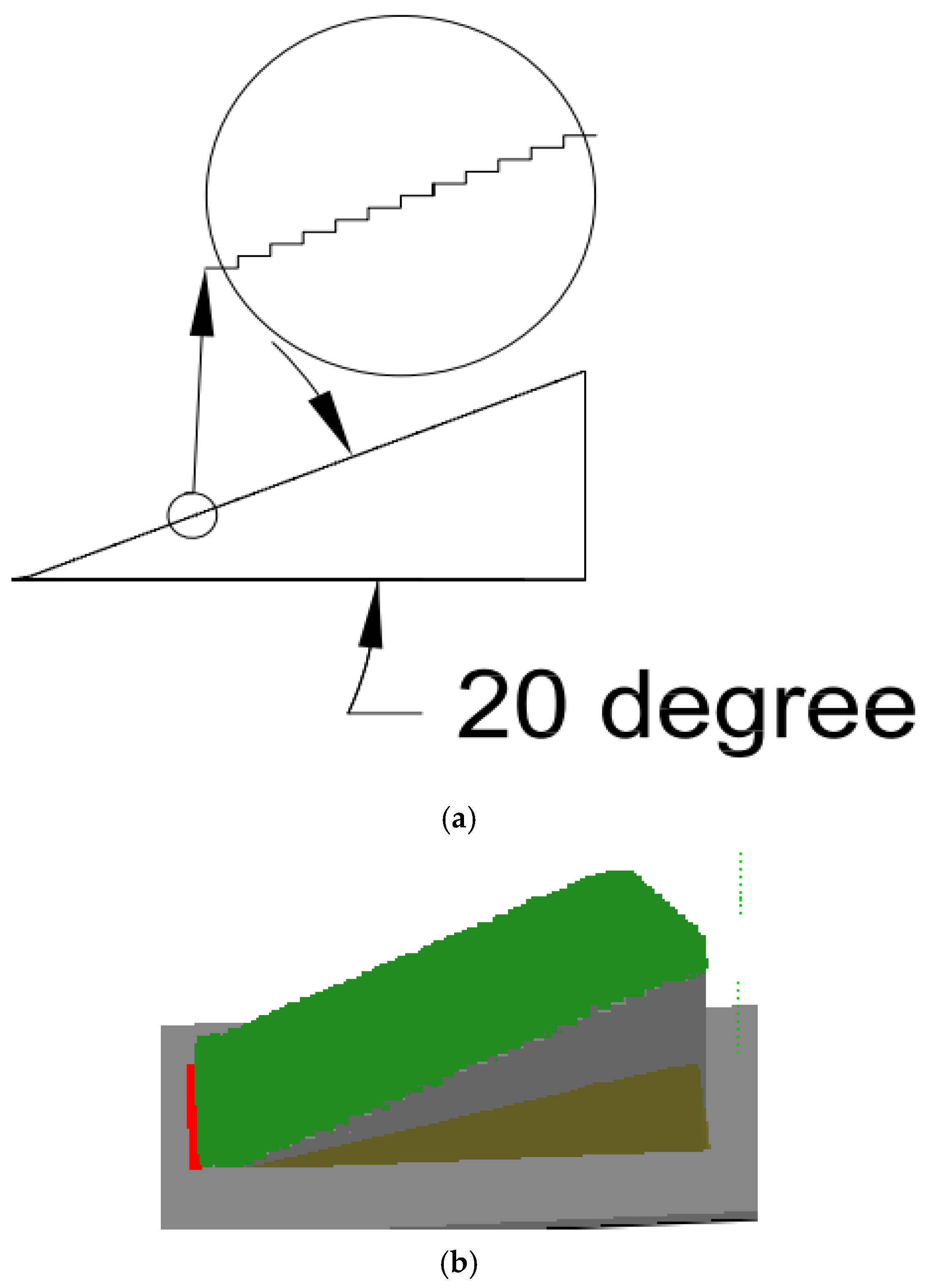
Figure 2a presents the analysis conducted for the 20° slope using the step method. The same analysis was applied to the 10° slope; we enlarged a section (highlighted within the circle) for better visualization. In these cases, all step faces are covered with vegetation, as illustrated in the Smokeview visualizations in Figure 2b. In our simulations with 10° and 20° slopes, we applied both available methods to examine the differences in their results. Each method’s rate of spread (ROS) was then compared with experimental data to determine which aligns more closely with observed values.

Figure 2. Step method analysis. (a) Analysis of the step method on a 20° slope, (b) Smokeview visualization for a 20° slope.

In the step method, different step sizes can be used to represent the slope, with smaller steps providing a more detailed approximation of the terrain. However, the step size cannot be smaller than the grid resolution, as the simulation grid dictates the minimum level of detail that can be captured. Therefore, in our simulation, the step size was set equal to the grid size to achieve the most refined representation of the slope while ensuring consistency with the computational resolution. The gravity method, as previously mentioned, relies on the X and Z gravity values specified in the FDS script file. The arctangent of the ratio of the X gravity parameter to the Z gravity parameter must equal the desired slope value. For the 10° slope, we set GVEC to −1.7, 0.0, −9.66 in the MISC line, while for the 20° slope, we used GVEC = −3.355, 0.0, −9.218. The negative sign indicates that the slope is directed in the positive X direction.

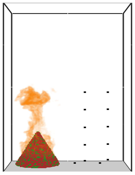
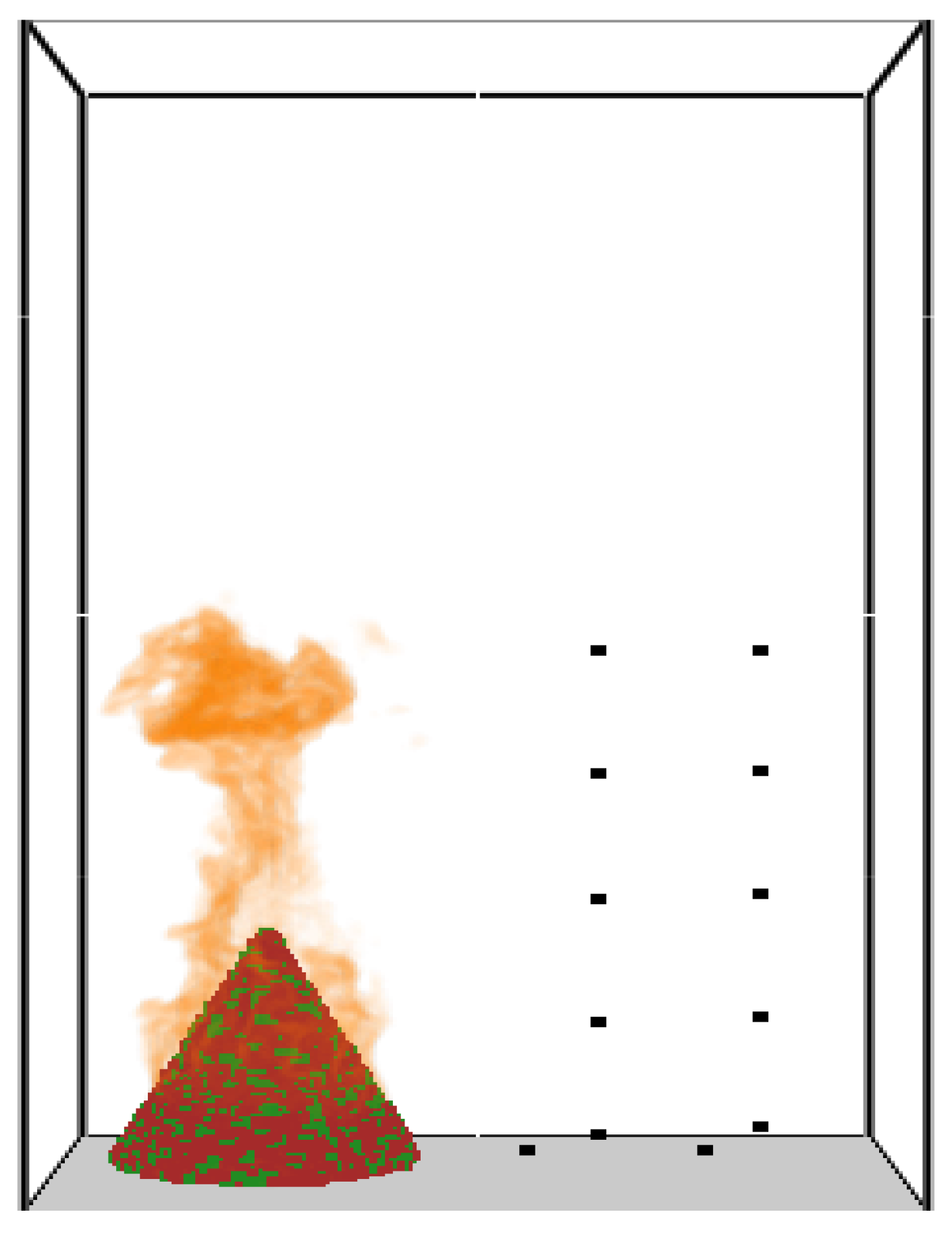
• Part II: Simulation of Single Douglas Fir Tree

The tree burning case selected for our study involves a 2 m-tall Douglas fir tree with 14% moisture content. Figure 3 presents a screenshot captured from the smoke view of the simulation results. In this scenario, our simulation setup closely adhered to the experimental methodology previously documented in Mell et al. [19]. The numerical model necessitates various thermo-physical properties for both the gas phase and the vegetative fuel. The specific properties required for the vegetative fuel are outlined in Table 2 and Table 3, which are taken from the original validation study. Table 3 presents the kinetic constants utilized in the simulation. It is to be noted that the thermo-physical properties used in Mell et al. [19] were not measured in their own laboratory for the same vegetation that was burned. These properties vary from species to species and even among the same species found in different geographical locations [43,44]. Therefore, we manually conducted an optimization study to obtain model-specific pre-exponential factor (A) and activation energy (E) values for vegetation and char by adjusting the values up to ±42% relative to the values used in Mell et al. [19]. The adjustment process was not random; instead, a structured parametric sweep was adopted in which A and E were varied incrementally within predefined bounds while monitoring key output indicators such as ignition timing, peak heat release rate, and overall mass-loss trends. The parameters were tuned iteratively and sequentially rather than all at once, allowing the influence of each parameter group to be observed before proceeding to the next. This adjustment range was selected to account for the inherent physical variability in pyrolysis kinetic parameters observed in wildland vegetation, which can arise from differences in species composition (e.g., cellulose, hemicellulose, and lignin content), moisture levels, plant age or condition (live vs. dead), and environmental factors [45]. The literature reports significant ranges in these parameters; for instance, activation energies (E) for biomass pyrolysis can vary by over 100% across species and conditions (e.g., 123–270 kJ/mol in distributed activation energy models), while pre-exponential factors (A) show logarithmic variations spanning several orders of magnitude [45]. The ±50% bound thus represents a conservative envelope to capture these uncertainties and derive effective parameters tailored to our model’s assumptions and fuel bed configuration, without exceeding typical reported deviations [46]. An advantage of this approach is its transparency and direct physical interpretability, as the sensitivity of the model’s response to each kinetic parameter can be explicitly observed. However, a limitation is that the procedure is computationally demanding and may not guarantee a mathematically unique optimum, since different parameter combinations can sometimes yield similar macroscopic fire behaviour. It is noted that various optimization algorithms exist in the literature to obtain A and E [47], including inverse modelling techniques that adjust parameters within bounded ranges to fit experimental data while accounting for measurement limitations (e.g., heating rates and off-gassing effects) [46].

Figure 3. The smoke view for the single fir tree simulation.

Table 2. Thermo-physical, pyrolysis, and burning parameters for Douglas fir trees [19].

	Parameter		Value
Gas phase	Mass-based heat of combustion		17,425 KJ/kg
	Fuel formula		C2.1H6.2O2.16
	A fraction of the consumed fuel mass is converted to soot		0.01
Solid phase	Fraction of virgin solid fuel converted to char		0.25
	Fraction of char converted to ash		0.04
	Specific heat capacity for water		4.22 KJ/kg C
	Moisture		14%
	Fuel density		514 Kg/m3
	Bulk density (total)		2.63 Kg/m3
	Foliage	Mass fraction	64%
		Surface-to-volume ratio	3940 m−1
	Small round wood	Mass fraction	11%
		Surface-to-volume ratio	2667 m−1
	Medium round wood	Mass fraction	10%
		Surface-to-volume ratio	888 m−1
	Large round wood	Mass fraction	15%
		Surface-to-volume ratio	500 m−1
	Fuel Geometry		cone
	Cone height		1.96 m
	Cone radius		0.85 m

Table 3. The kinetic constants used in the simulations.

	Kinetic Constant	Value	Reference
GENERIC VEGETATION	Pre-exponential factor log(A)	4 s−1	[19] +25%
	Activation Energy E	61,041 J/mol	[19]
CHAR	Pre-exponential factor log(A)	4.66 s−1	[19] +42%
	Activation Energy E	61,200 J/mol	[19] −10%

In our study, the validation process involves comparing the experimental mass-loss rate and experimental heat flux with the corresponding values obtained from the simulation. The mass-loss rate is a key parameter, as it arises from the combined processes of heat generated by gas-phase combustion, the convective and radiative transfer of this heat to the vegetation, and the subsequent thermal degradation of the vegetation (mass loss), which can produce additional fuel vapour for sustained burning. The mass-loss rate is automatically calculated within the simulation, while the heat flux is measured using sensors placed at specific locations mirroring those in the real experiment. Ten sensors are strategically positioned to measure the heat flux. Five sensors are placed at a radius of 2 m from the centre of the tree at heights of 0.2 m, 1.2 m, 2.3 m, 3.4 m, and 4.5 m from the reference zero z level. Additionally, five sensors are positioned at a radius of 3 m from the centre, also spanning the same height levels from the ground. All of these sensors can be seen in Figure 3 as black dots; this setup ensures comprehensive coverage and accurate data collection for heat flux analysis. Overall, this validation approach combines automated simulation calculations for mass-loss rate with real-time sensor data collection for heat flux, providing a robust framework for evaluating the accuracy and reliability of the simulation model.

3. Grid Size Analysis

3.1. Surface Fire Simulations

Before conducting any sensitivity analysis for grid resolution, we examined the extinction length scale, as suggested in Morvan [15] for the FE vegetation model. According to Morvan, the grid resolution should be finer than the extinction length, determining using the following equation:

$${\delta }_{\mathrm{R}}={\displaystyle \frac{4}{{\alpha }_s{\sigma }_s}}$$

(1)

where

• ${\delta }_{\mathrm{R}}$ is the extinction length (m);
• ${\alpha }_s$ represents the packing ratio, which is the volume fraction occupied by the vegetation;
• ${\sigma }_s$ denotes the surface area-to-volume ratio.

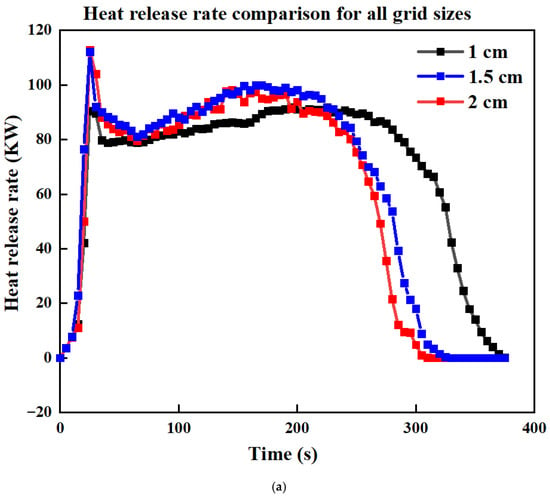
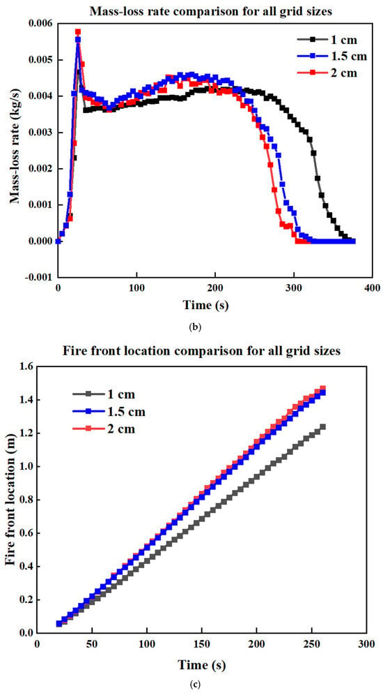
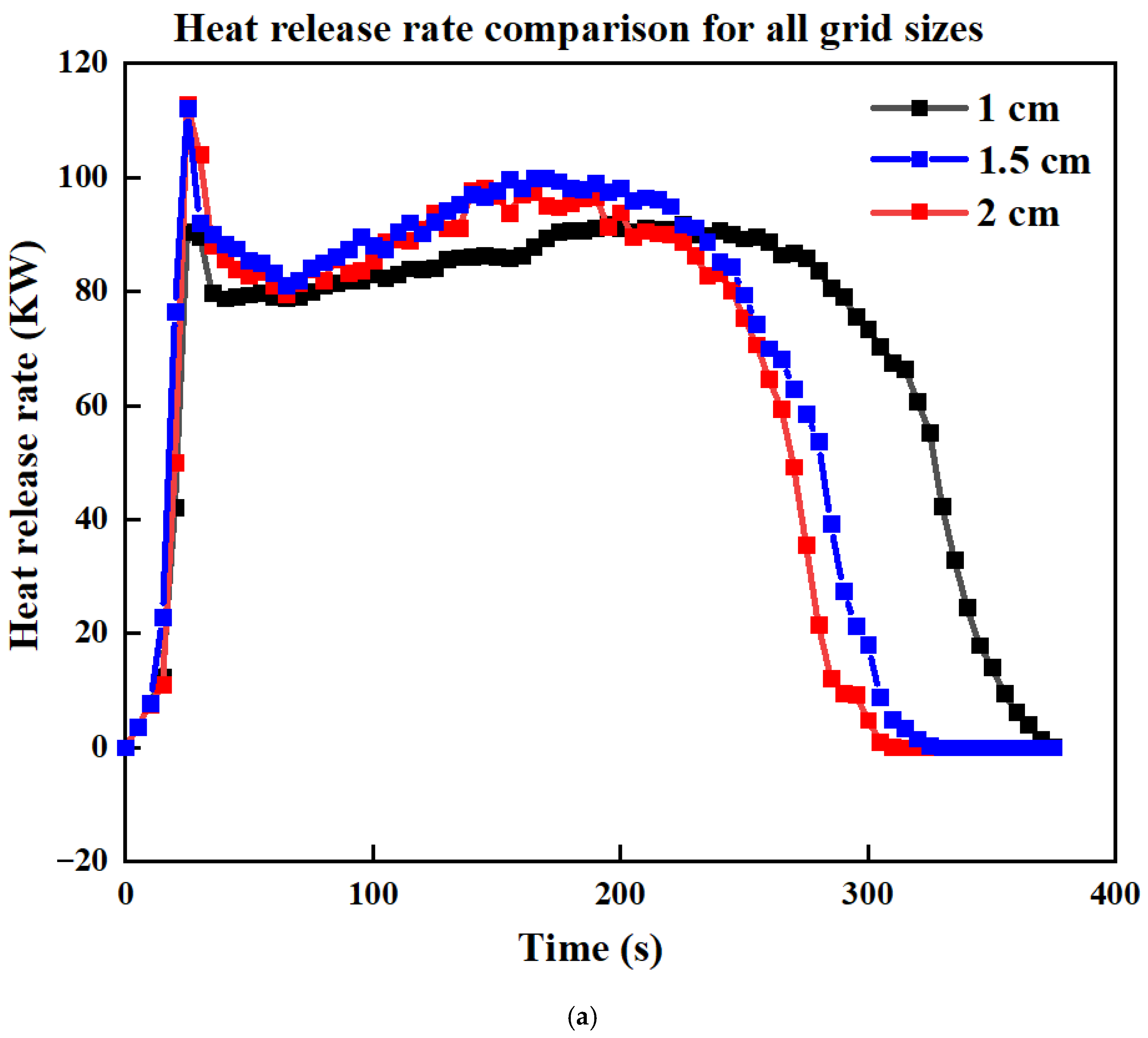
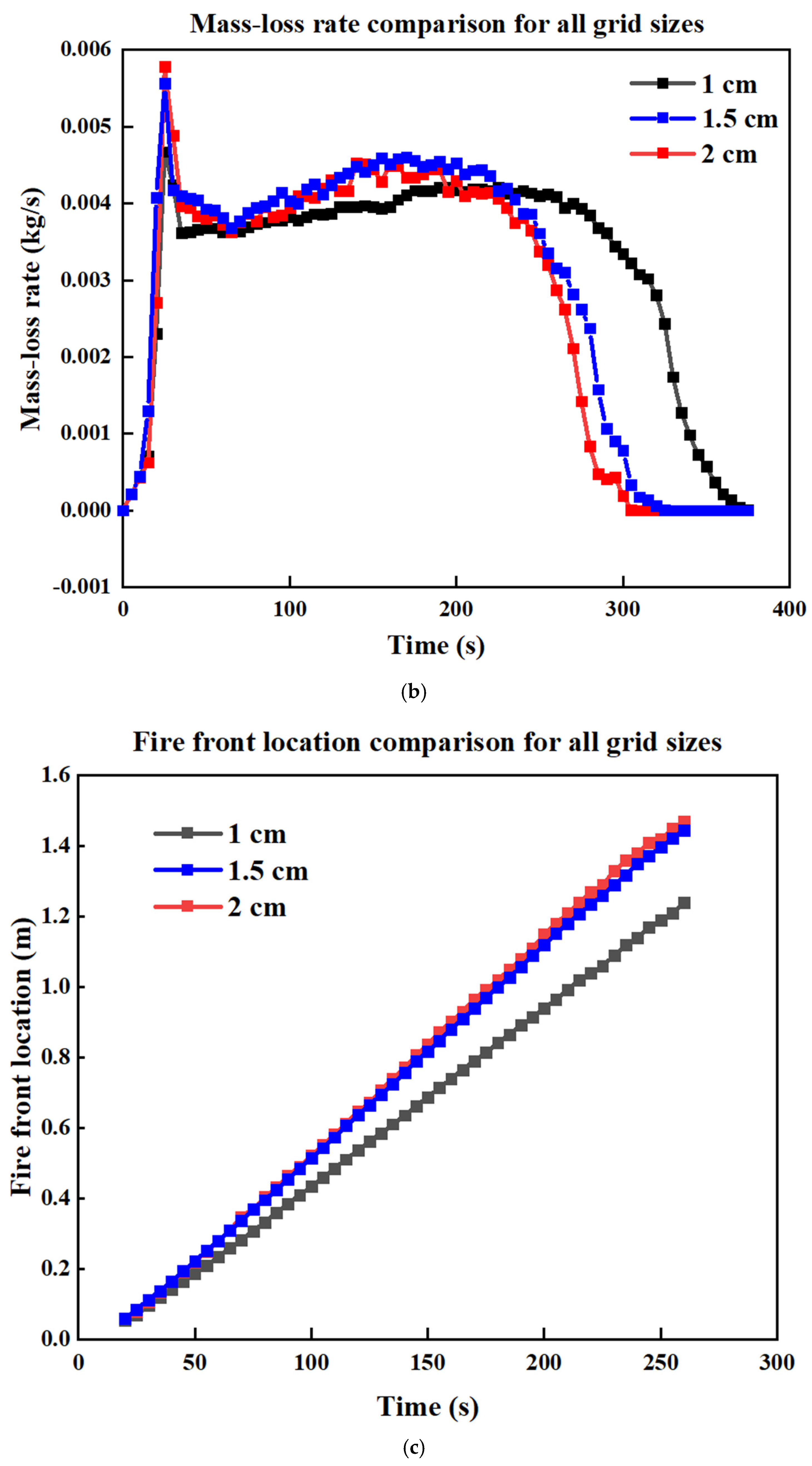
The extinction length for our vegetation was calculated to be 4.6 cm. To evaluate the influence of grid resolution, we compared the heat release rate (HRR), mass-loss rate (MLR) and fire front location across three grid sizes—2 cm, 1.5 cm and 1 cm—as shown in Figure 4. The results indicate that the 1.5 cm and 2 cm grid sizes produce similar MLRs, HRRs, and fire front locations, indicating that reducing the grid from 2 cm to 1.5 cm does not improve the results. In contrast, the 1 cm and 2 cm grid sizes produce similar HRR and MLR values up to approximately 225 s. Beyond this time, some differences emerge in the absolute values, although the overall trend remains consistent between the two grids. Reducing the grid size below 1 cm would be computationally difficult due to the substantial resource demands. In Figure 4c, which compares the fire front location, we observe that the grid size of 1 cm exhibits a different slope compared to the 1.5 cm and 2 cm grids.

Figure 4. Comparison of (a) HRR (b) MLR, and (c) fire front location for four cases with different grid sizes, for the surface fire simulations.

The Grid Convergence Index (GCI) [48] is a way to measure how sensitive simulation results are to changes in grid resolution. It is used in grid refinement studies to assess how the results are converging towards a solution, and can be expressed as follows:

$$\mathrm{G}\mathrm{C}\mathrm{I}={\mathrm{F}}_{\mathrm{s}} {\displaystyle \frac{{\in }_{rms}}{ r^q-1}} \times 100$$

(2)

The value q shows the order of the numerical method used (in this study, q = 2 for a second-order method), and F_s is a safety factor, usually between 1.25 and 3 [48]. The grid refinement ratio r is calculated using the number of cells in two simulations, one with a finer mesh (N1) and one with a coarser mesh (N2), using the formula r = (N1/N2)^1/3. The symbol ${\in }_{rms}$ stands for the root mean square of the relative error, which gives a basic idea of how much the results change with finer grids. Based on the fire front location, we calculated the GCI between the 2 cm, 1.5 cm, and 1 cm grids, as presented in Table 4.

Table 4. Grid convergence percentage difference for the surface fire simulations.

Coarse Grid/Fine Grid	GCI Value
2 cm/1.5 cm	9.17%
1.5 cm/1 cm	44.25%
2 cm/1 cm	20.11%

The GCI analysis shows a relatively low value of 9.17% between the 2 cm and 1.5 cm grids, as expected with the close result observed in Figure 4c. However, the GCI rises significantly to 44.25% between the 1.5 cm and 1 cm grids; for the 2 cm to 1 cm comparison, the GCI falls in between at 20.11%. Although the 2 cm and 1.5 cm grids give very similar results, the GCI with 1 cm shows very different values and this discrepancy arises due to the grid refinement ratio r used in the GCI equation. Since there is minimal difference in the results between the 1.5 cm and 2 cm grids, while noticeable differences remain between these grids and the 1 cm resolution, we selected the 1 cm and 2 cm grid resolutions for all simulation cases. As outlined in the Methodology section, the step size is set equal to the grid size. Accordingly, for cases with a 1 cm grid size, the step size is 1 cm, while for cases with a 2 cm grid size, the step size is 2 cm.

Finally, after completing the grid size analysis and the domain sensitivity analysis, as shown in Appendix A, and determining all simulation parameters, we will proceed to simulate 10 cases; each case is designated by slope (Z for zero slope, S10 for 10° slope, and S20 for 20° slope), slope method (G for gravity and S for step), and grid resolution (1C for 1 cm and 2C for 2 cm). For example, case S10S2C represents a 10° slope with the step method and a 2 cm grid. Further details regarding the sensitivity analysis conducted for the surface fire simulations are provided in Appendix A.1.

3.2. Single Douglas Fir Tree

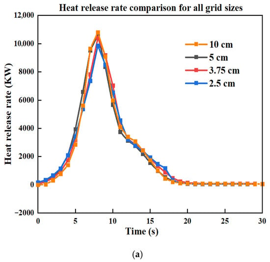
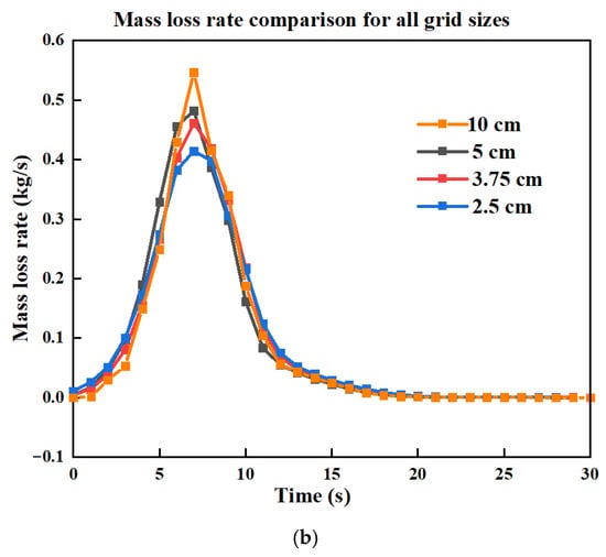
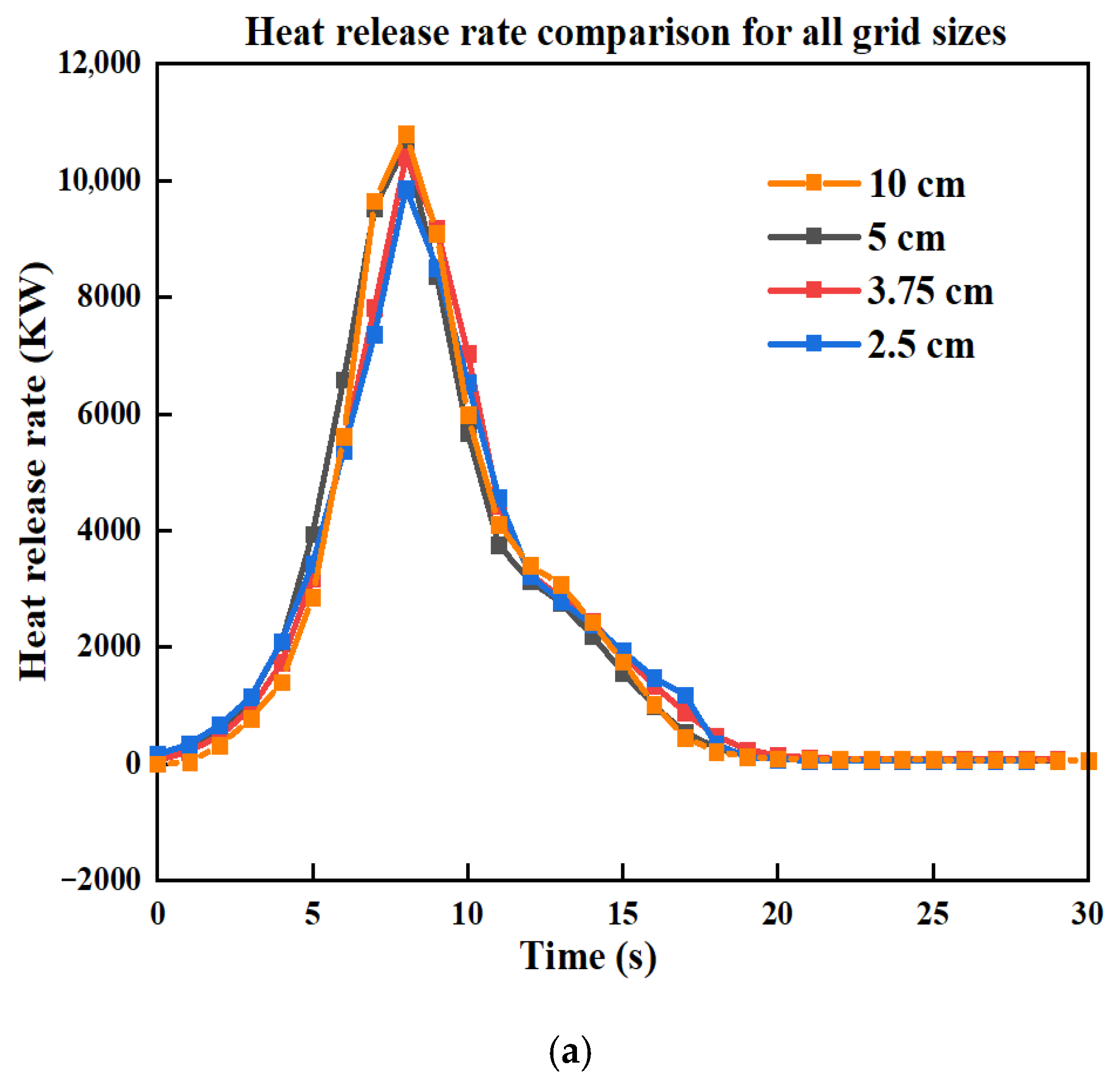
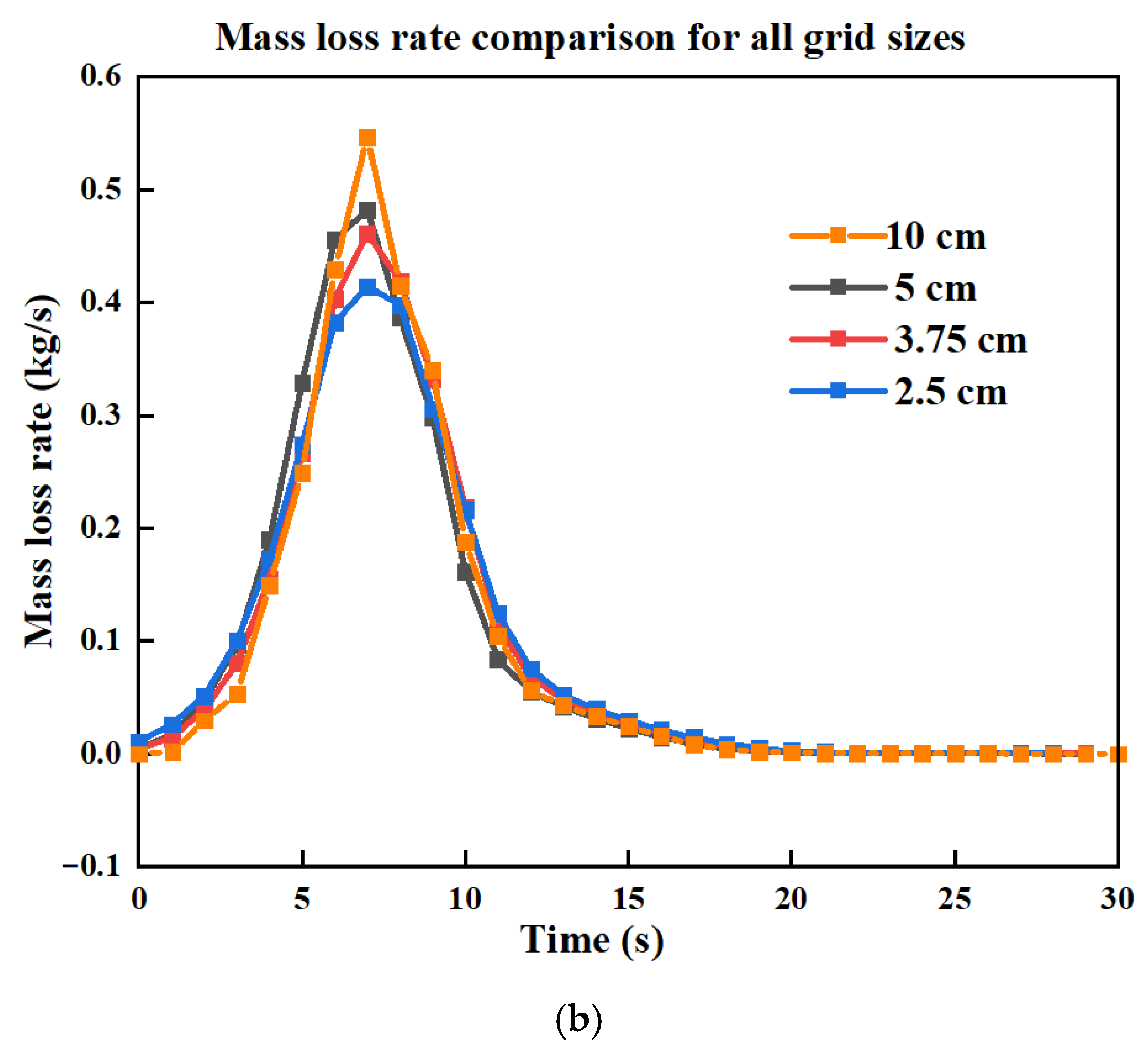
To evaluate the influence of grid resolution, we first followed Morvan’s [15] suggestion to determine the extinction length for Douglas fir tree vegetation, which was found to be 39 cm. Based on this, we selected grid sizes smaller than this threshold and compared the heat release rate (HRR) and mass-loss rate (MLR) across four grid sizes—10 cm (the grid size used in the original validation), 5 cm, 3.75 cm, and 2.5 cm—as shown in Figure 5. For the HRR in Figure 5a, the differences between all grid sizes were minimal. However, for the MLR, noticeable differences emerged between the grid sizes. The 5 cm and 3.75 cm grids produced similar results, with MLR values lower than those of the 10 cm grid but higher than those of the 2.5 cm grid. Comparing the 2.5 cm and 3.75 cm grids, their MLR curves closely align, differing by only 9% in peak MLR value. Consequently, we selected 2.5 cm as the appropriate grid size. Furthermore, using a 2.5 cm grid instead of 3.75 cm improves the ability to capture complex physics more realistically and enhances the resolution of turbulent structures and smaller eddies. Given the close results in Figure 5, we calculated the GCI for r = 2 only and present the values in Table 5. It shows that GCI values of 30–50% in terms of the HRR with r = 2 can be considered well-converged results. Further details regarding the sensitivity analysis conducted for the single Douglas fir tree are provided in Appendix A.2.

Figure 5. (a) Comparison of HRR and (b) MLR for three cases with different grid sizes, for the single Douglas fir tree simulation.

Table 5. Grid convergence percentage difference for single Douglas fir tree.

Coarse Grid/Fine Grid.	GCI Value %
10 cm/5 cm	30.36%
5 cm/2.5 cm	48.27%

4. Results and Discussion

4.1. Surface Fire

4.1.1. Rate of Spread

We began by comparing fire spread over a flat pine needle fuel bed (0° slope). The rate of fire spread is a key factor in comparing the simulation results with experimental data to validate our model. To determine the rate of fire spread (ROS), we employed a method involving the extraction of forefront locations, represented as a threshold surface temperature, along the central axis of the burnable pine plot at various time intervals from the boundary file. This extraction process was performed using MATLAB version (R2023b) and can also be automated by inserting a device into the simulation file to obtain this location. By plotting fire front locations against time, we can derive the ROS, which is quantified as the slope of the curve. This provides insights into the dynamic behaviour of fire spread over time. The ROS was then compared with experimental results from Yang et al. [35].

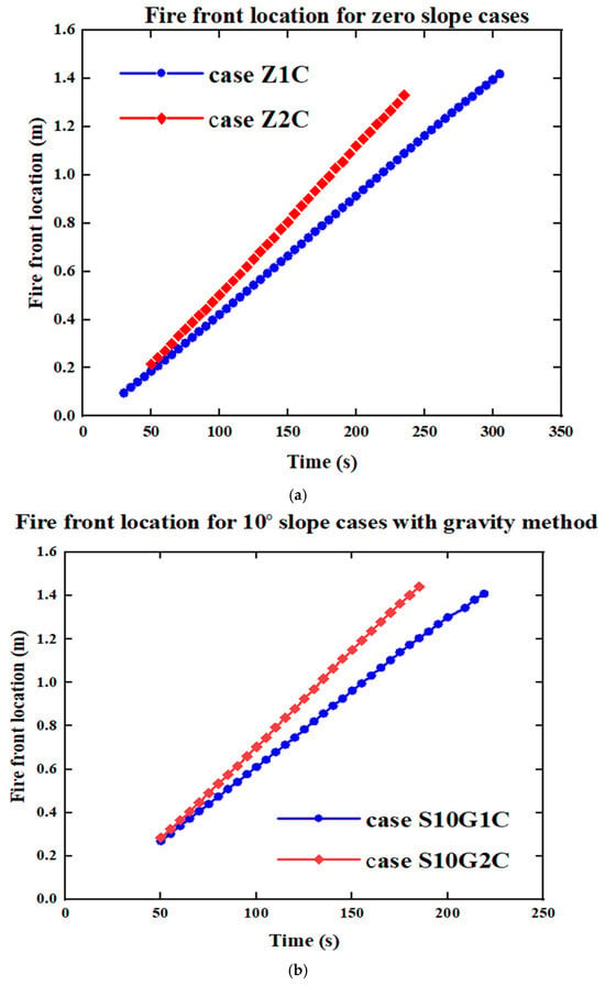
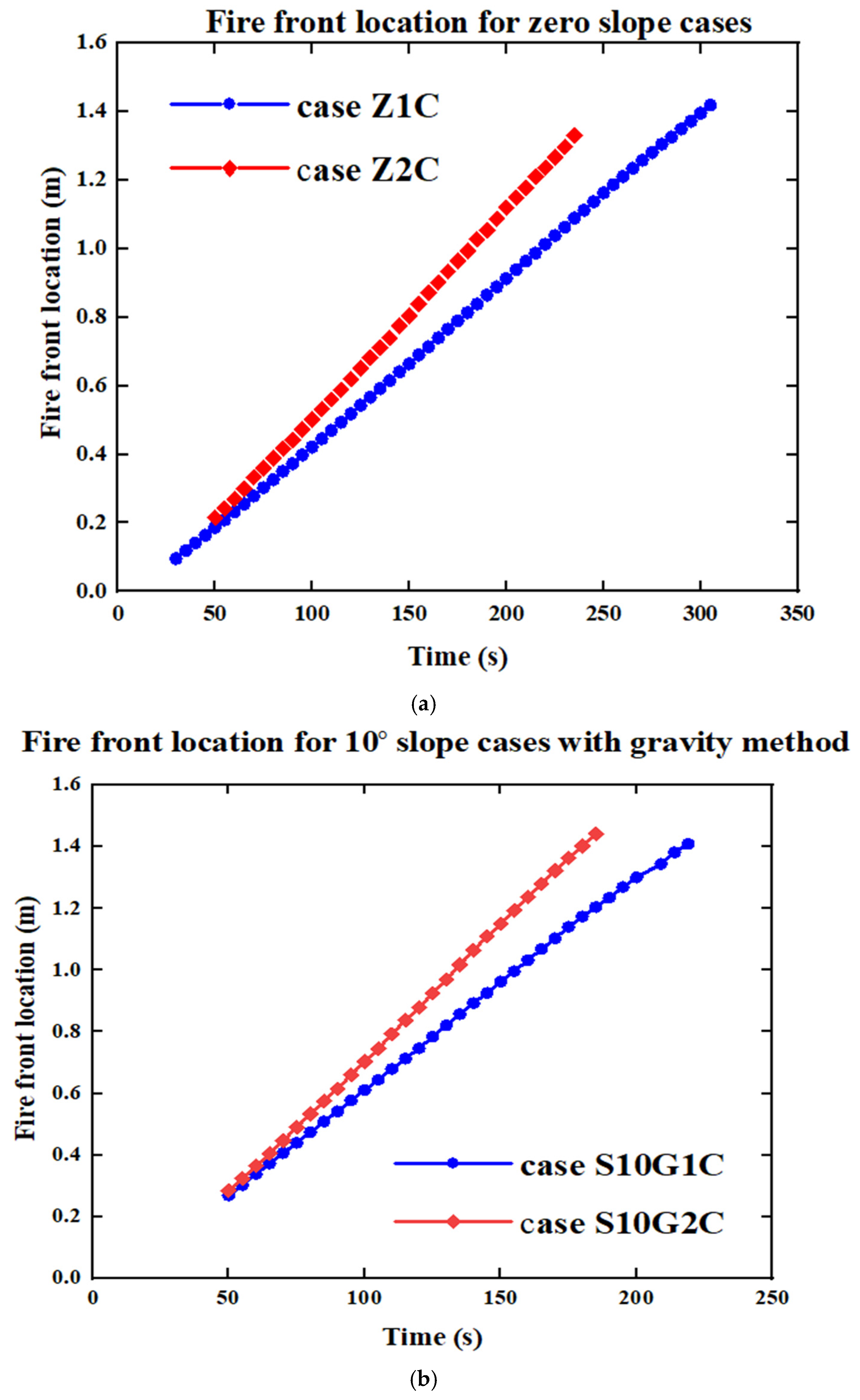
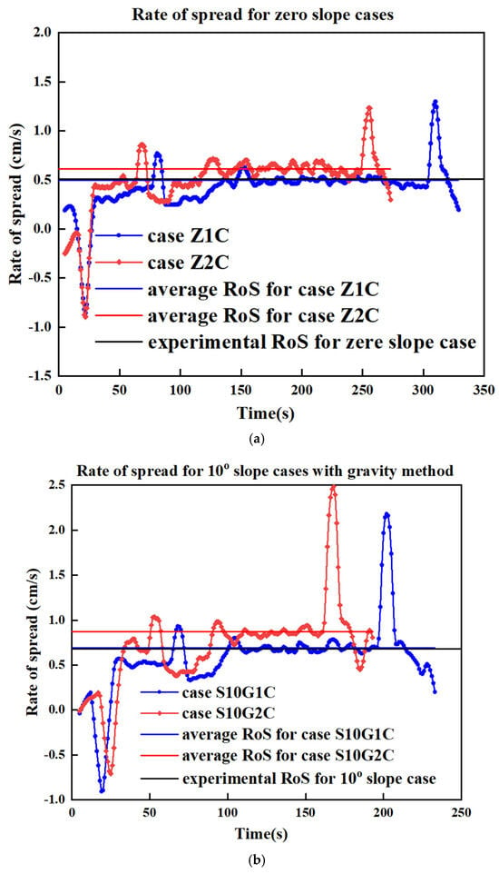
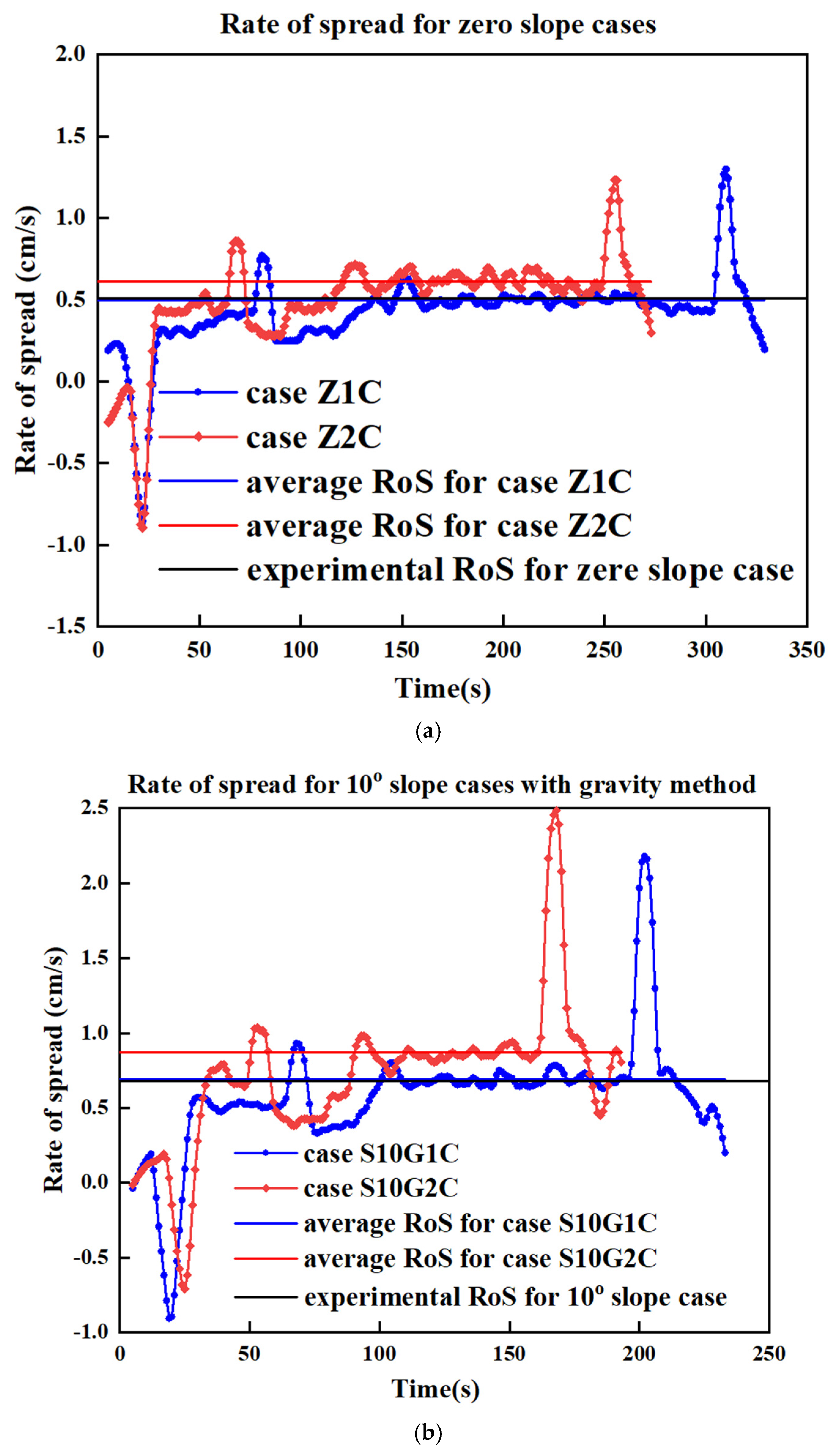
In Figure 6a, fire front location results are presented. The slopes of these lines represent the ROS and are presented in Figure 7a. For a grid size of 1 cm, the ROS was 0.5 cm/s, whereas for a grid size of 2 cm, the ROS increased to 0.61 cm/s. These values closely align with the experimental value of 0.507 cm/s. The relative error for the 1 cm grid case is 1.38%, indicating a strong agreement between the simulation and experimental results. In contrast, the 2 cm grid case shows a relative error of 20.3%. As expected, a finer grid resolution improves the accuracy of the results.

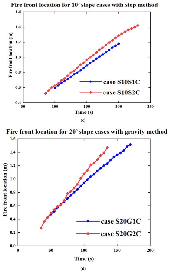
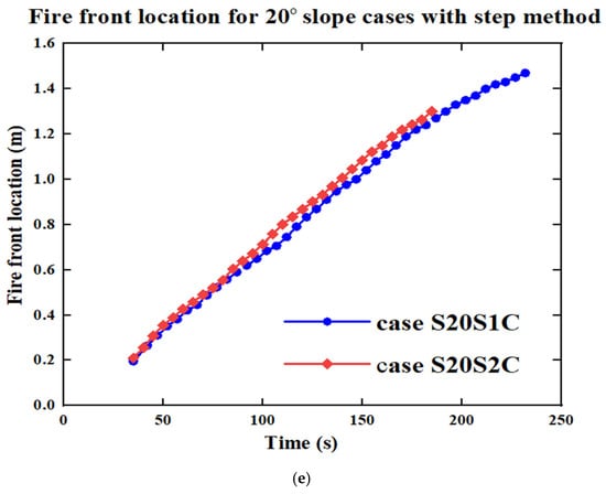
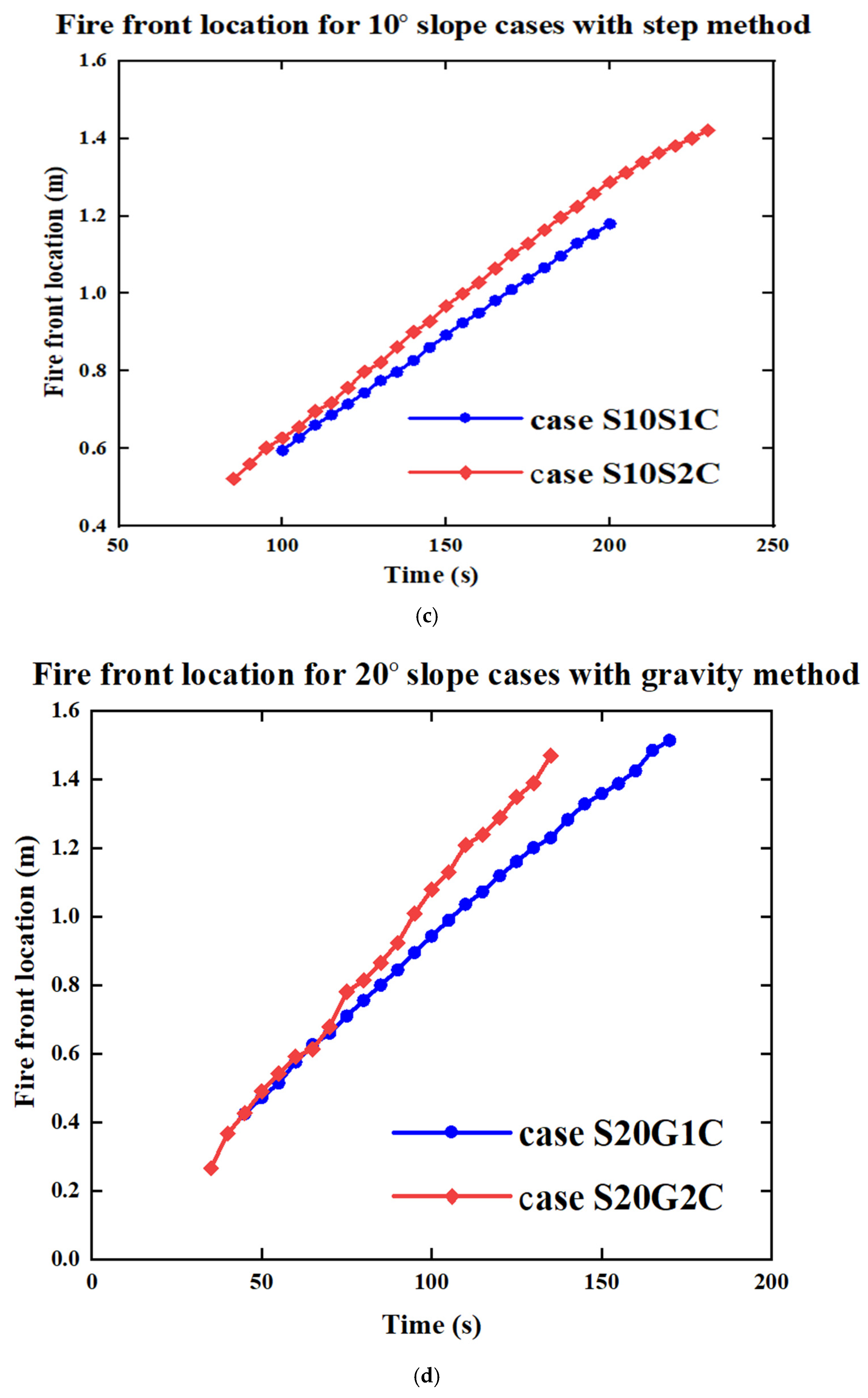
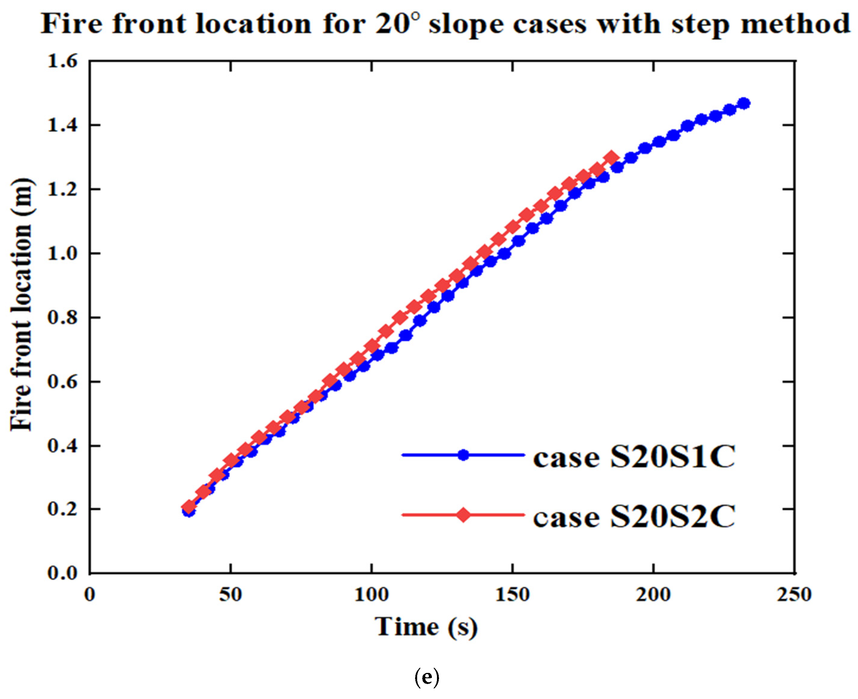
Figure 6. Fire front positions for all simulated cases at each time step. The blue lines represent cases with a fine grid size of 1 cm, while the red lines correspond to cases with a coarse grid size of 2 cm. The blue lines exhibit a lower slope, indicating a reduced rate of fire spread compared to the red lines. (a) Zero slope, (b) 10° slope with gravity method, (c) 10° slope with step method, (d) 20° slope with gravity method, and (e) 20° slope with step method.

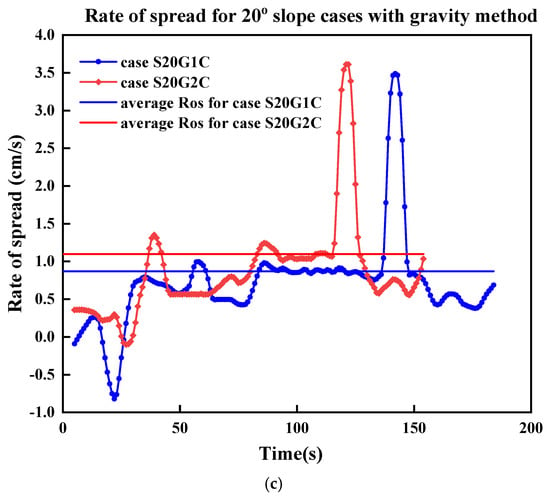
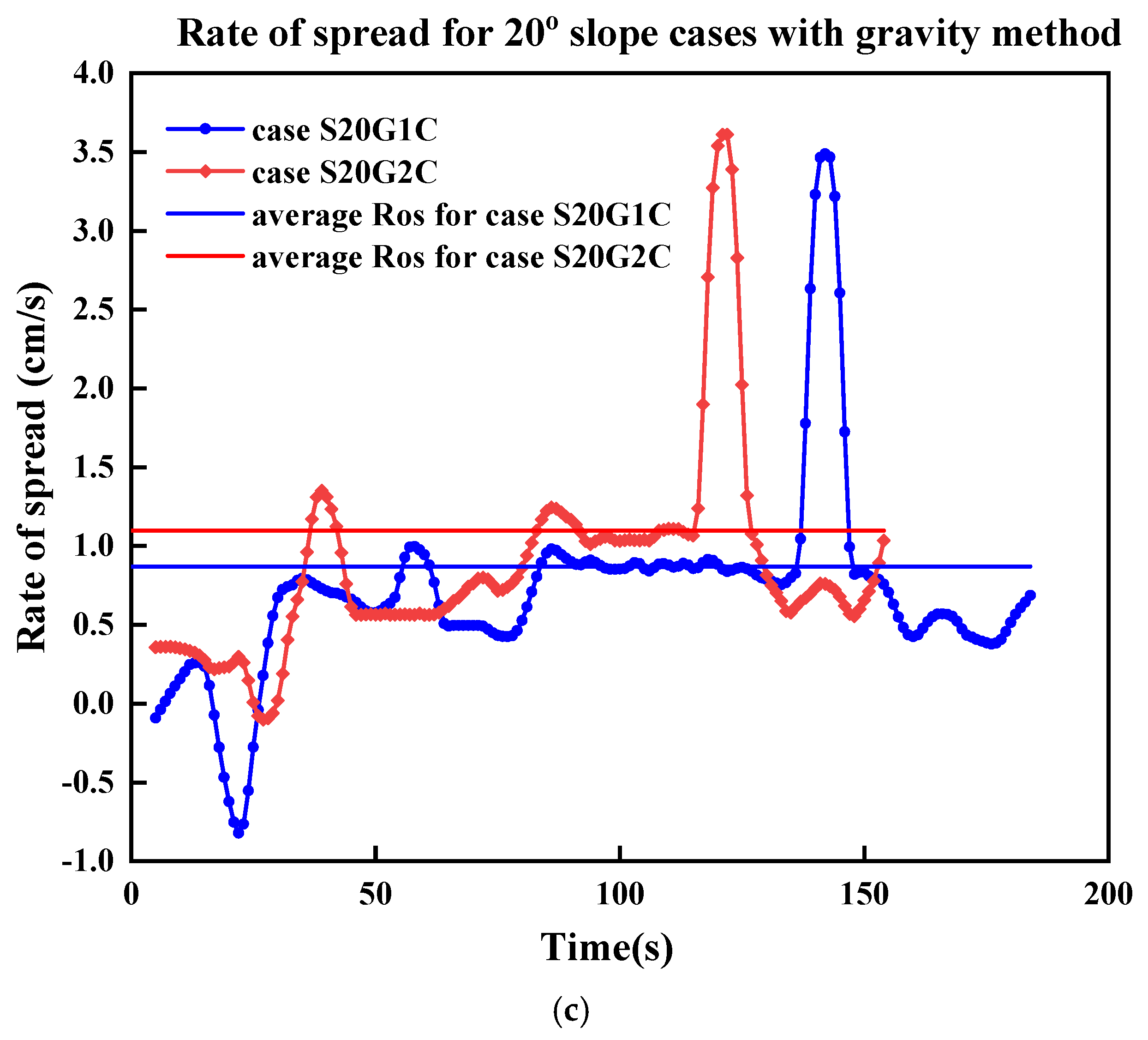
Figure 7. Rate of fire spread for simulated cases at each time step, where blue lines (1 cm grid) show a lower rate of spread compared to red lines (2 cm grid) across (a) zero slope cases, (b) 10° slope cases using the gravity method, and (c) 20° slope cases using the gravity method; the blue and red horizontal lines represent the average ROS for the 1 cm and 2 cm grid sizes, respectively, while the horizontal black line represents the experimental ROS value from Yang et al. [35].

After validating the model on flat terrain, we introduced inclined surfaces (10° and 20° slopes) to examine the FDS’s reliability to simulate upslope fire spread. Figure 6b,c illustrate the fire front location for simulations with a 10° slope using the gravity and step methods, respectively. In both cases, a finer grid resolution results in a lower slope of the fire front progression, consistent with observations from the zero-slope cases. ROSs have are shown in Figure 7b for the gravity method. For the 10° slope, the gravity method with a 1 cm grid predicted an ROS of 0.69 cm/s, closely matching the experimental value of 0.679 cm/s with only a 1.6% error. The 2 cm grid overestimated the ROS (0.87 cm/s), with a relative error of 28.1%. Once again, as expected, a finer grid can increase the accuracy of the results. The step method produced lower ROS values (0.59 cm/s for the 1 cm grid and 0.66 cm/s for the 2 cm grid). The difference with the experimental value is not significant in absolute values. The better result with a coarser grid may attributed to the right amount of air flow from the sides. In the stepped-slope configuration, the discretized geometry introduces small vertical discontinuities that interact with the flow field. With a very fine grid, these discontinuities can locally restrict lateral entrainment and modify the near-surface velocity field, slightly reducing the predicted ROS. A coarser grid, on the other hand, smooths these micro-scale obstructions and allows a more uniform side-air entrainment, which, in this specific configuration, happened to compensate for other numerical biases and yielded a closer ROS to the experimental value. This behaviour should not be interpreted as a general advantage of coarse grids, but rather as a case-specific numerical compensation effect. Overall, the gravity method with a 1 cm grid size yields the best agreement with experimental results for this slope condition. Table 6 presents a summary of the ROS results along with the relative errors for the simulated cases.

Table 6. The summary of the ROS results.

Case	Simulated ROS (cm/s)	Experimental ROS (cm/s)	Relative Error %
Z1C	0.5	0.507	1.38%
Z2C	0.61	0.507	20.3%
S10G1C	0.69	0.679	1.6
S10G2C	0.87	0.679	28.1
S10S1C	0.59	0.679	13.1
S10S2C	0.66	0.679	2.7
S20G1C	0.87	Not Available	Not Available
S20G2C	1.1	Not Available	Not Available
S20S1C	0.72	Not Available	Not Available
S20S2C	0.73	Not Available	Not Available

Figure 6d and Figure 6e depict the fire front location for simulations with a 20° slope using the gravity and step methods, respectively. Notably, this specific scenario is not included in the experimental data; however, it was simulated to evaluate the models’ performance under varying conditions. For the gravity method, the ROS increases by 26% when transitioning from the 10° to the 20° slope for the 1 cm grid case and by 26.4% for the 2 cm grid case. Similarly, for the step method, the ROS increases by 22% for the 1 cm grid case and by 10.6% for the 2 cm grid case. This difference can be attributed to the fact that in the gravity method, the only variable affecting the ROS is the grid size, leading to a consistent increase across different resolutions. In contrast, the step method involves both grid size and step size variations, resulting in different ROS increments for each grid resolution. Additionally, as observed in the 10° slope scenario, there is minimal difference in the ROS between the 1 cm and 2 cm grid sizes when using the step method. Furthermore, consistent with trends seen in the zero-slope and 10° slope cases, simulations with a finer (1 cm) grid resolution produce lower ROS values compared to those with a course (2 cm) grid.

Compared to the step method, the gravity method exhibits a greater sensitivity to grid resolution. This indicates that the step method may offer computational efficiency for slope simulations, as it performs consistently without requiring a finer grid.

The fluctuations in the ROS shown in Figure 7—including distinct peaks and drops—are not observed in Figure 6. These variations indicate transient disturbances in fire propagation that were not accounted for in the ROS calculations in Figure 6, where only a smoothed average value was considered, neglecting turbulence effects. The two horizontal lines in each plot indicate the average ROS value for each case, corresponding to the slope of the curves in Figure 6. For cases using the step method, our current code is unable to compute the ROS at each time step due to the complexity introduced by multiple steps and layers. This limitation highlights the need for further code modifications to enable accurate time step-based ROS calculations for such cases. Across all cases shown in Figure 6, the ROS for simulations with a 2 cm grid size is consistently higher than that of the corresponding 1 cm grid cases, a trend also observed in Figure 6.

4.1.2. Flame Length

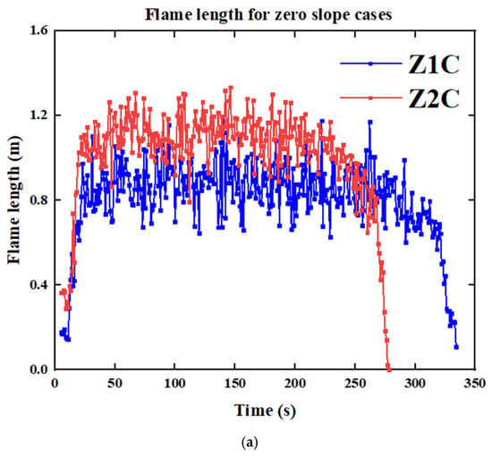
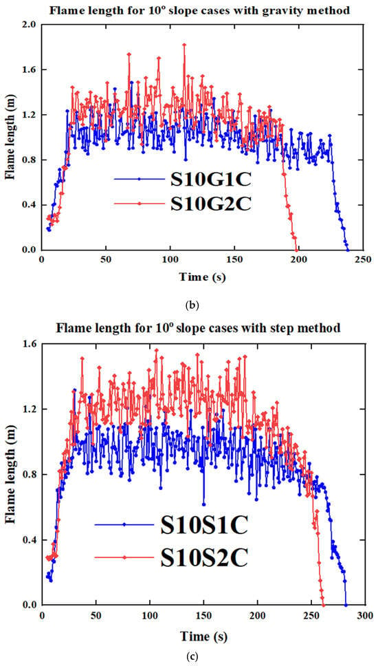
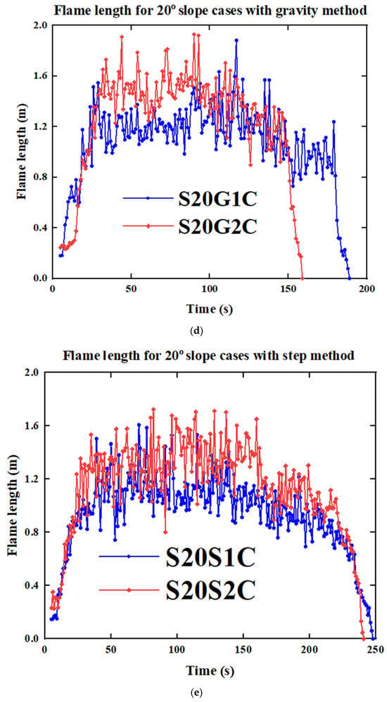
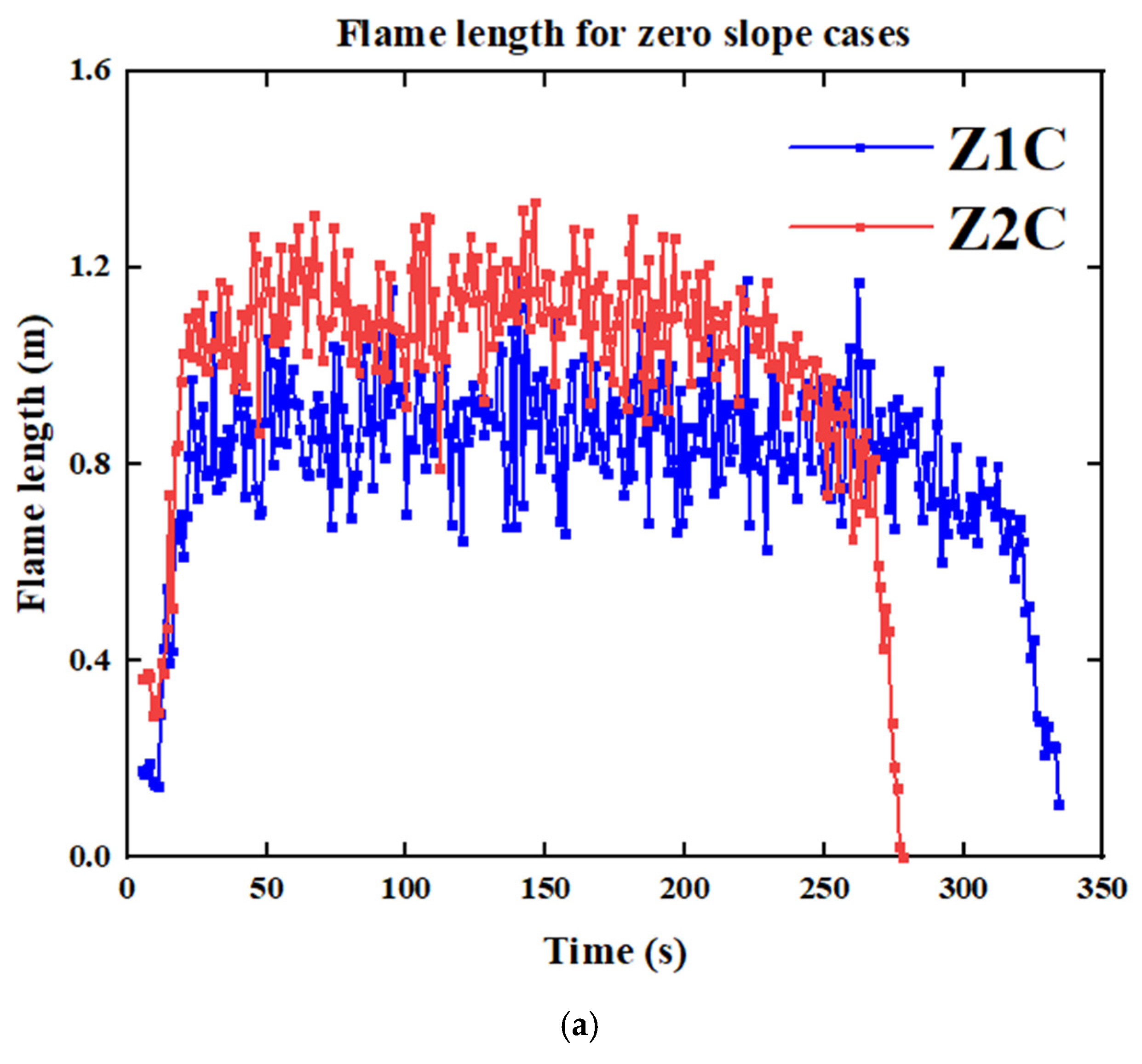
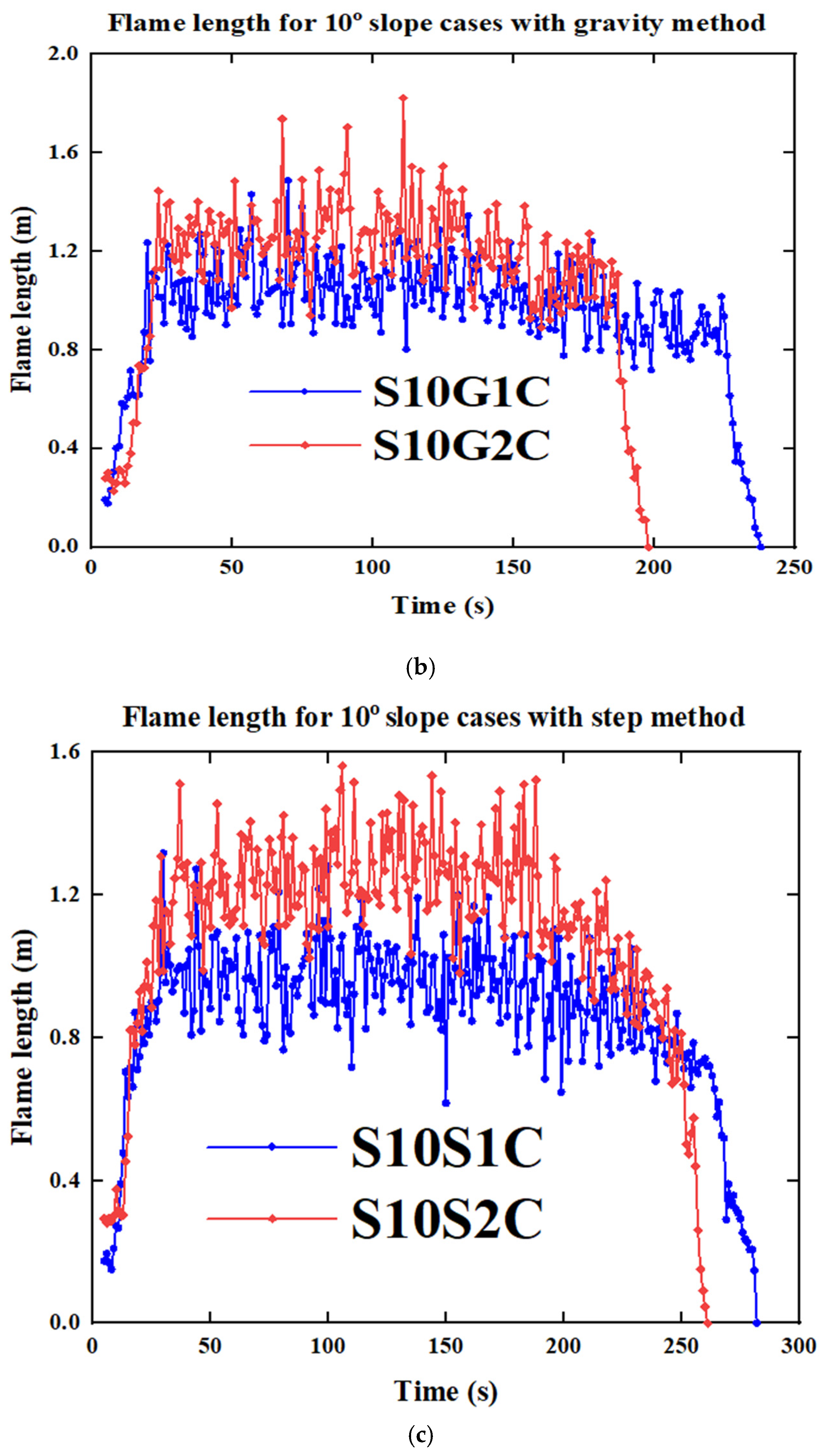
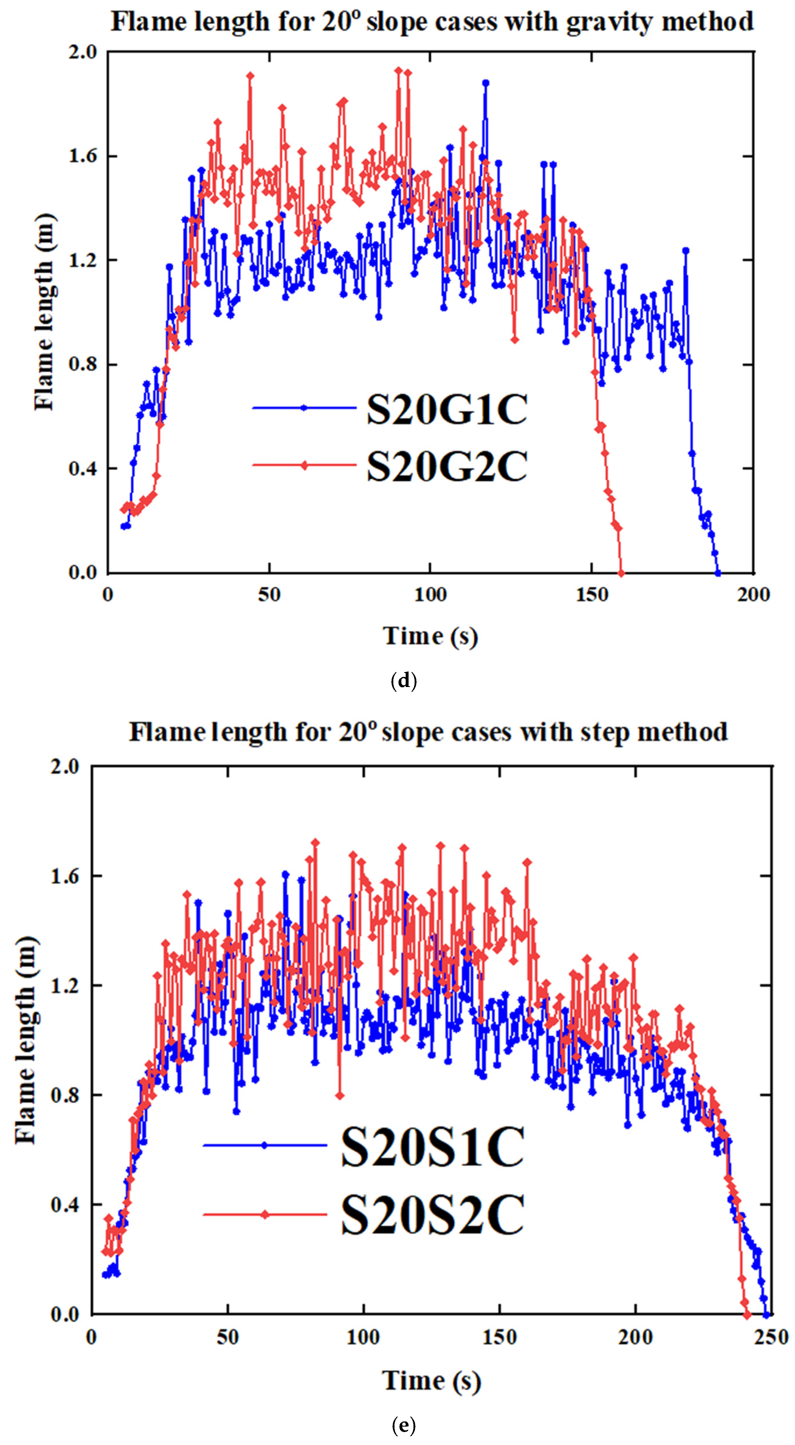
We analyzed flame length, an important parameter for fire intensity, by comparing the experimental results with the simulation. Table 7 presents the experimental and the average range of the simulated flame length values for the zero-slope and 10° slope scenarios. The relative error between the simulation and experimental results ranges from 6.6% to 20.7%, demonstrating the model’s capability to simulate surface fire with outcomes closely matching reality. The flame length is figured out by looking at the heat release rate (HRR) data from the slice file along the centreline at each moment (y = 0). At every time step, we analyze the HRR data and use the highest observed HRR value as a threshold value to create a black-and-white image. In this image, areas inside the threshold value boundary are marked as one, and those outside are marked as zero. Following the approach of Cobian-Iñiguez et al. [49], we use MATLAB version (R2023b) to fit an ellipse to this binary image at each time step. This ellipse is fitted using the moments of the nonzero region in the image, ensuring its shape reflects the spread of the region. The flame length is then calculated based on the major axis of this fitted ellipse, representing the distance from the centre of the flame base to the tip of the flame.

Table 7. Experimental and simulated flame length for the zero-slope and 10° slope scenarios.

Case	Experimental Value (m)	Average Simulation Value (m)	Relative Error
Z1C	0.952	0.6–1	15.9%
Z2C	0.952	1–1.3	20.7%
S10G1C	1.018	0.9–1.3	8%
S10G2C	1.018	1–1.4	17.8%
S10S1C	1.018	0.8–1.1	6.6%
S10S2C	1.018	1.1–1.35	20.3%

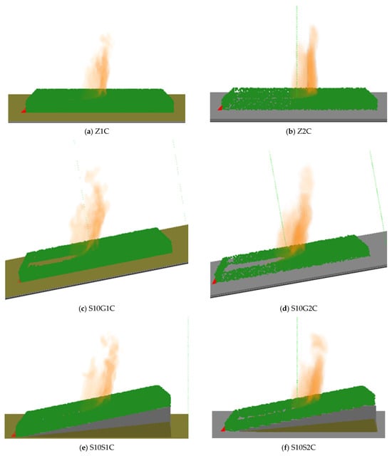
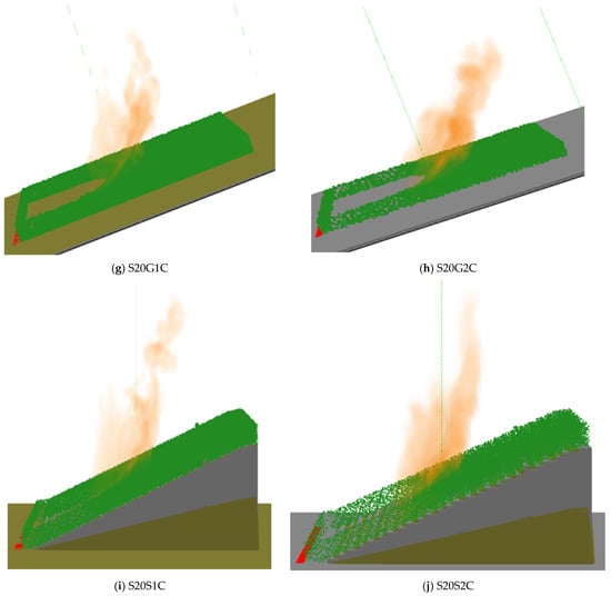
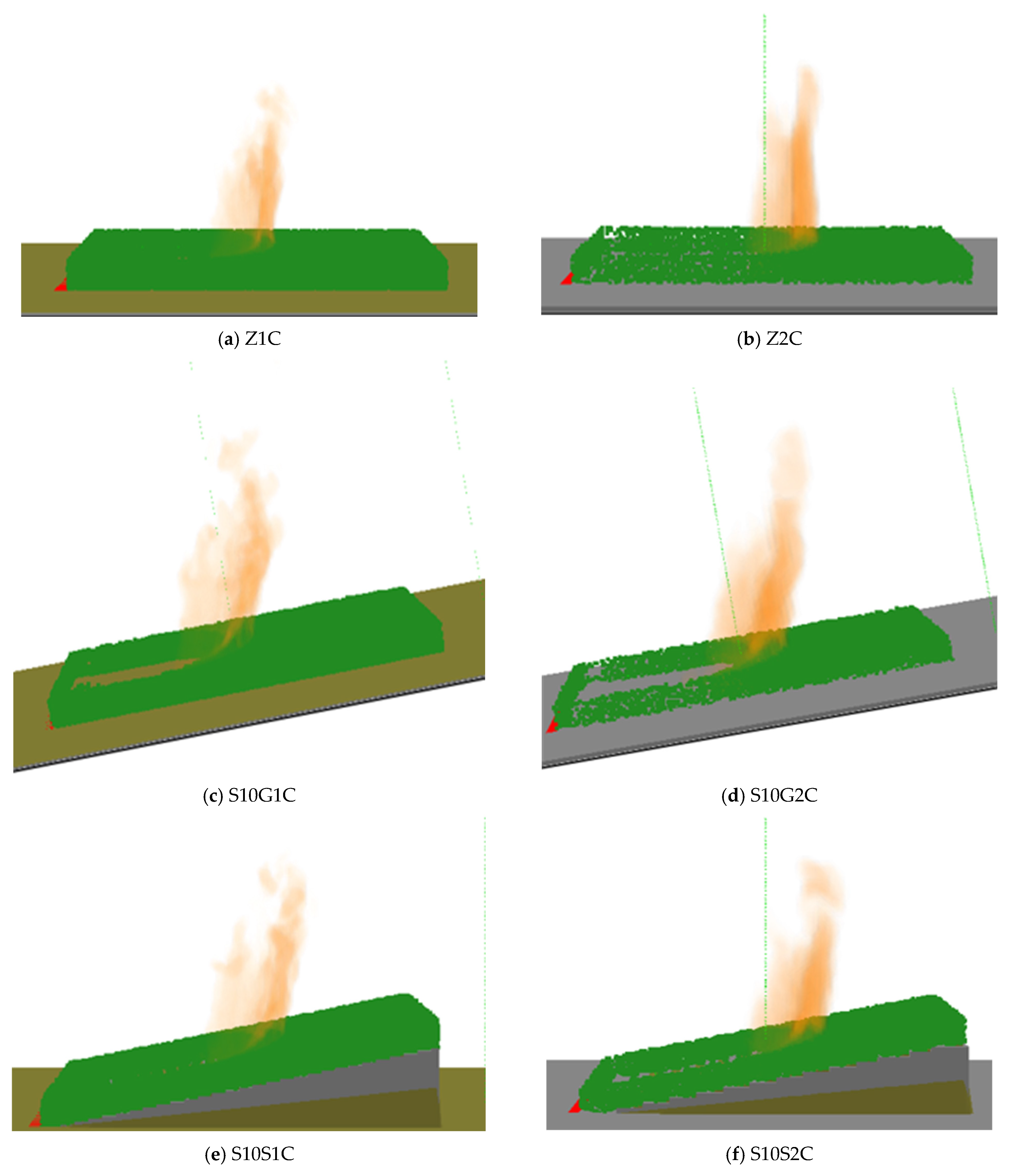
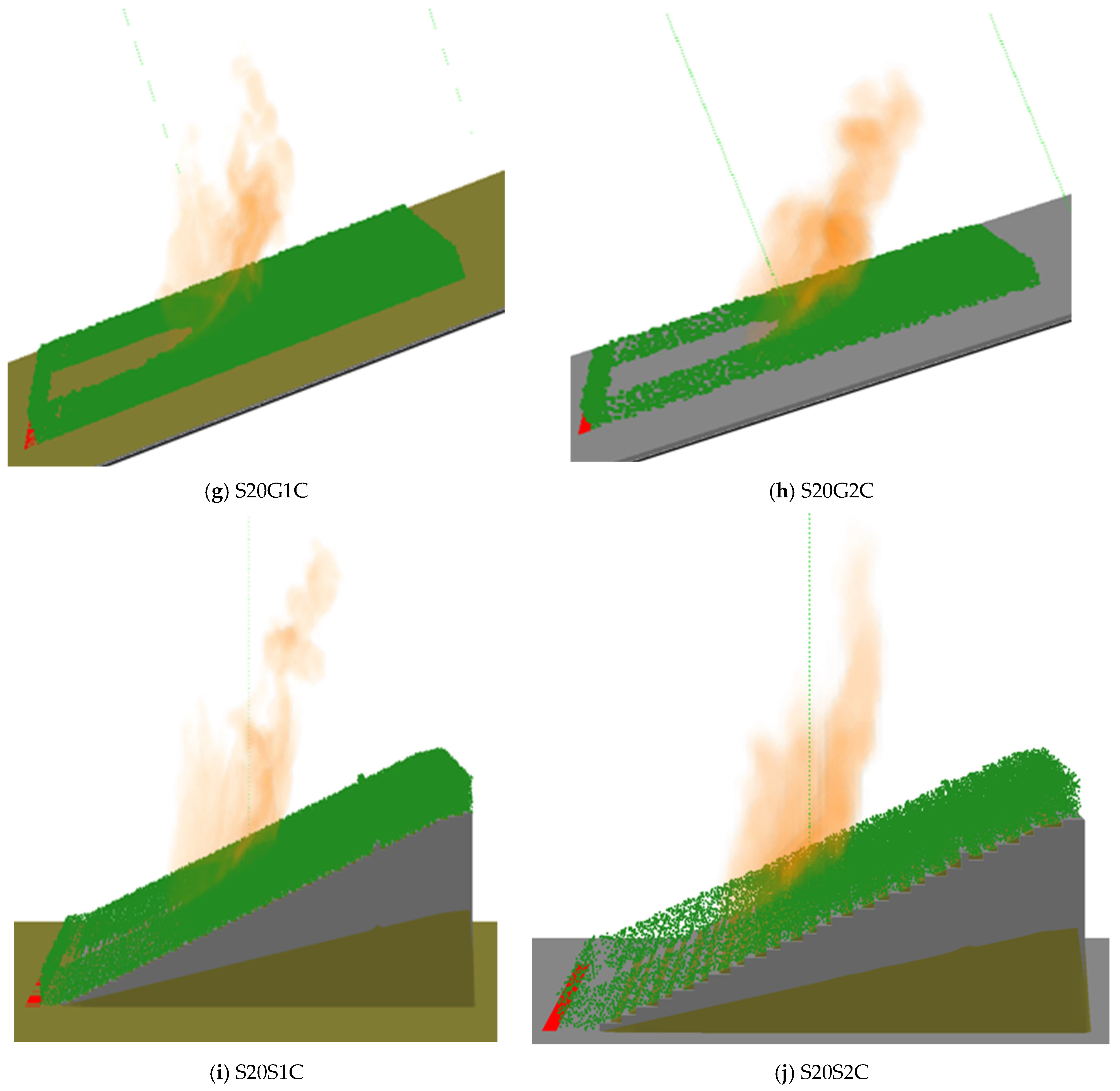
Figure 8 illustrates the flame length for all simulated cases, showing that cases with a coarse grid size exhibit a higher flame length than those with a finer grid size across all scenarios and higher relative errors. This behaviour is attributed to the influence of grid resolution on turbulence, entrainment, and heat transfer. Coarse grids under-resolve turbulent eddies and air entrainment, leading to reduced mixing with ambient air, higher localized temperatures, and elongated flames [32]. Additionally, numerical diffusion and averaging effects in coarse-grid simulations exaggerate flame length by failing to capture fine-scale turbulence and radiative heat loss [50]. In contrast, finer grids more accurately represent turbulence and heat dissipation, leading to shorter and more realistic flame structures [51]. These effects are further illustrated in Figure 9, which provides a smoke view comparison of flame lengths across all simulated cases, highlighting the grid-dependent variations in flame behaviour.

Figure 8. Flame length for all simulated cases at each time step. The blue lines represent cases with a fine grid size of 1 cm, while the red lines correspond to cases with a coarse grid size of 2 cm. The blue lines exhibit a lower flame length compared to the red lines. (a) Zero slope, (b) 10° slope with gravity method, (c) 10° slope with step method, (d) 20° slope with gravity method, and (e) 20° slope with step method.

Figure 9. Flame length visualization from the smoke view for all simulated cases, showing the influence of grid resolution on fire behaviour, with coarser grids resulting in higher flame lengths across all scenarios.

4.2. Single Douglas Fir Tree

4.2.1. Mass-Loss Rate

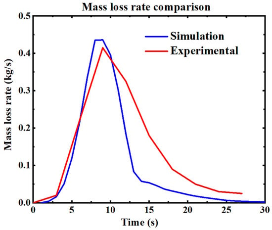
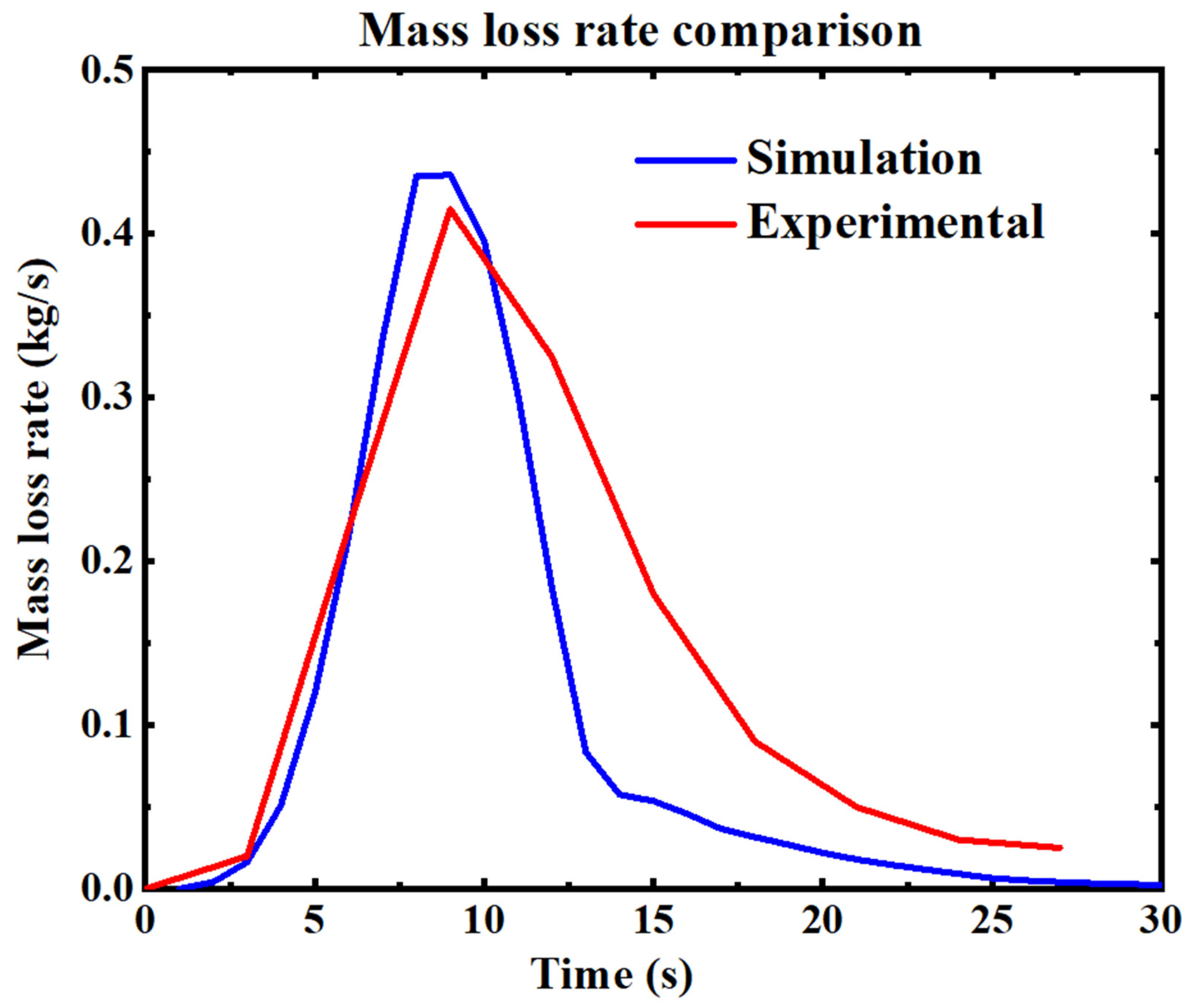
After evaluating surface fire behaviour, we now focus on single-tree fire simulations. Figure 10 illustrates the average mass-loss rate observed in the tree-burning experiments (red line) alongside the results from the FDS simulations (blue line). The mass-loss rate represents a key metric arising from the coupled interaction between fire and fuel as the flames progress through the vegetation. The experimental data and simulation results show similar trends, with both curves exhibiting a rapid increase to a peak MLR, followed by a gradual decline.

Figure 10. Comparison of mass-loss rate between simulation and experimental data. The red curve represents the experimental mass-loss rate from Mell et al. [19], while the blue curve corresponds to the simulated mass-loss rate.

The simulated peak MLR for the simulation slightly underestimates the experimental value. Still, it closely matches the overall profile, particularly in the decay phase, indicating that the model captures the essential dynamics of the combustion process. This alignment suggests that FDS 6.8 effectively replicates the thermal degradation behaviour and fuel consumption rate observed in the experiment, supporting the model’s validity for similar fire scenarios. The peak mass-loss rate from the experimental data is 0.415 kg/s; in comparison, the peak mass-loss rate from the simulation is 0.436 kg/s, resulting in a 5% error compared to the experimental value, which indicates that the FDS effectively captures the burning rate during the most intense burning phase, and suggests that the model accurately represents the thermal degradation processes at peak fire activity. The total mass loss is 3.9 kg in the experimental data and 2.93 kg in the simulation, yielding a 24.8% error relative to the experimental results. While a 24.8% error is relatively high, it might still be within an acceptable range, depending on the experimental setup and the complexity of the fire behaviour being modelled.

4.2.2. Heat Flux

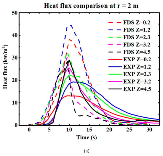
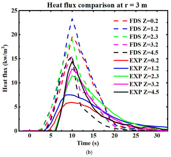
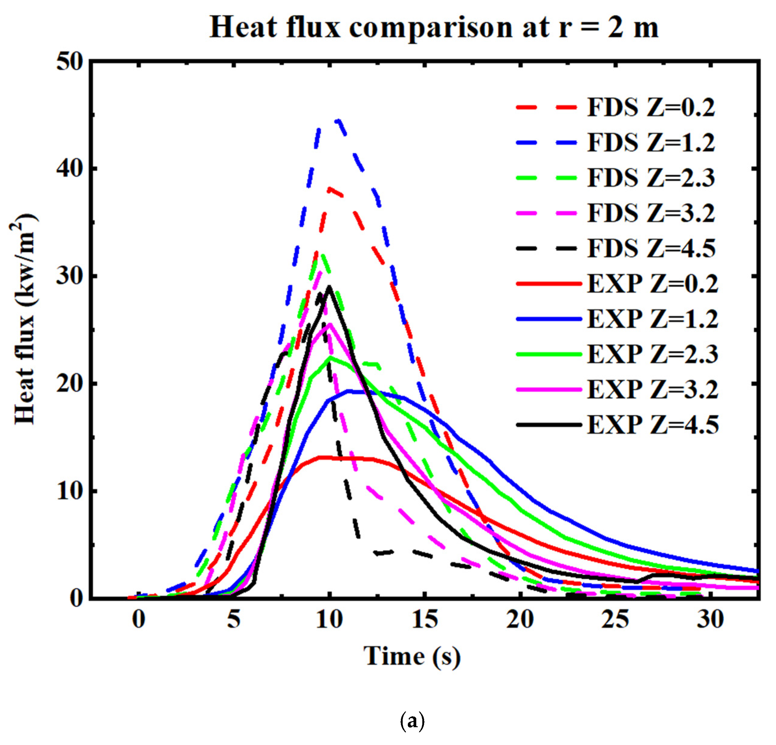
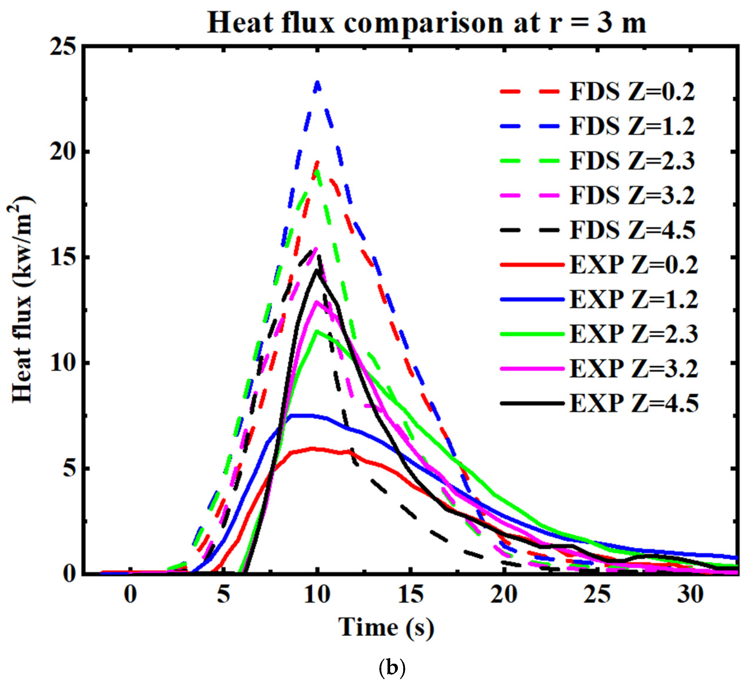
Radiation can be a crucial factor in the spread of fires at the wildland–urban interface (WUI) by preheating fuels in advance of the fire front. This preheating facilitates piloted ignition, either through direct flame contact or potentially from firebrands produced by burning vegetation or structures. Figure 11 presents the time history of the total heat flux measured in the experiment (solid lines) and the incident radiant flux predicted by the FDS (dashed lines). The heat flux was recorded at two horizontal distances from the centre of the tree (x = 2 m and x = 3 m), with measurements taken at five heights above the base of the tree trunk (z = 0.2 m, 1.2 m, 2.3 m, 3.4 m, and 4.5 m), as previously described.

Figure 11. Comparison of heat flux between simulation and experimental data. The dashed curves represent the simulation results, while the solid curves correspond to the experimental data from Mell et al. [19]: (a) at 2 m from the tree centre and (b) at 3 m from the tree centre.

In the FDS, the term “incident radiant flux” refers to the radiant flux in the gas phase. From the experimental data, it is observed that maximum heat flux increases with measurement height. This trend is attributed to the fire occupying a larger view angle at higher measurement points. The FDS successfully replicated this trend at the lower heights (z = 0.2 m and z = 1.2 m), though the simulated heat flux values are higher than the experimental values. At the higher levels (z = 2.3 m, z = 3.2 m, and z = 4.5 m), the simulated and experimental heat flux values are more closely aligned compared to the lower levels, indicating improved accuracy of the simulation at these heights. This alignment at higher levels suggests that the FDS can capture radiant flux at elevated points, although discrepancies remain at lower levels. This may be due to the idealization of the cone shape (see Figure 3), leading to a larger amount of fuel near the ground in the simulation compared to the actual tree-burning experiments.

Although the validation presented in this study was conducted at laboratory scale, the underlying fire–flow interactions resolved by the FDS are governed by non-dimensional parameters that enable cautious extrapolation to larger scales. Fire behaviour can be classified into buoyancy-dominated and wind-dominated fires, characterized by the Byram number (or, equivalently, the Froude number). These non-dimensional quantities characterize the relative contributions of vertical fluid motion due to buoyancy and inertial forces due to the driving wind [52]. Dimensionless parameters are valued in fluid dynamics as they offer the possibility of self-similar flow and thus allow scaling of laboratory-scale results to predict larger-scale flow behaviour. While the simulation of the Navier–Stokes equations conserves fluid mass, momentum, and energy, offering the prospect of applying dimensionless scaling, the heat transfer mechanisms—radiation and convection—do not non-dimensionalize in the same manner as the Navier–Stokes equations. Therefore, extrapolating results from laboratory scale to field scale is not straightforward. Nonetheless, the observations of [52] suggest that some scaling with the Byram number does occur.

5. Conclusions

This study presents a validation analysis of the FDS (6.8) for two scenarios. In the first scenario, we simulated surface fires on slopes of 0°, 10°, and 20°, using two methods for upslope fire spread: gravity and step methods. We compared our simulations for the 0° and 10° slopes with experimental data. For the 0° slope, the relative error in the ROS between the simulation and the experiment was 1.38% for a 1 cm grid and 20.3% for a 2 cm grid, demonstrating that finer grids produce more accurate results. For the 10° slope (gravity method), the relative error in the ROS was 1.6% for a 1 cm grid and 28.1% for a 2 cm grid. However, for the 10° slope (step method), the relative error was 13.1% for a 1 cm grid and 2.8% for a 2 cm grid.

Based on these results, finer grids produce more accurate simulations for surface fires on flat terrain (0° slope) and for 10° slopes using the gravity method. However, for the 10° slope with the step method, reducing the grid size leads to less improvement in accuracy compared to the gravity method. By comparing the simulated flame length with experimental results, we observe that the relative error ranges from 6.6% to 15.9% for simulations with a fine grid, whereas it increases from 17.8% to 20.7% for a coarse grid. As expected, using a finer grid improves the accuracy of flame length predictions compared to a coarser grid.

In the second scenario, we compared the simulation of a single Douglas fir tree with experimental results. The relative error was 5% for the peak mass-loss rate and 24.8% for the total mass-loss rate. Additionally, we observed that the simulated heat flux trends at 2 m and 3 m from the tree centre closely followed the experimental data. Based on the obtained results, it can be concluded that the Fire Dynamic Simulator (FDS6.8) has been adequately validated. This validation supports confidence in using FDS6.8 for future simulations, where accurate and trusted results are anticipated.

Appendix A.1. Surface Fire Simulations

We will conduct sensitivity analyses for the surface fire simulations on the ignition line intensity and domain size, in addition to the grid size sensitivity analysis already conducted in Section 3.1. This analysis will initially be conducted for the zero-slope case, and the finalized parameters will subsequently be applied to simulations involving other slope angles.

Appendix A.1.1. Ignition Line Intensity (HRRPUA)

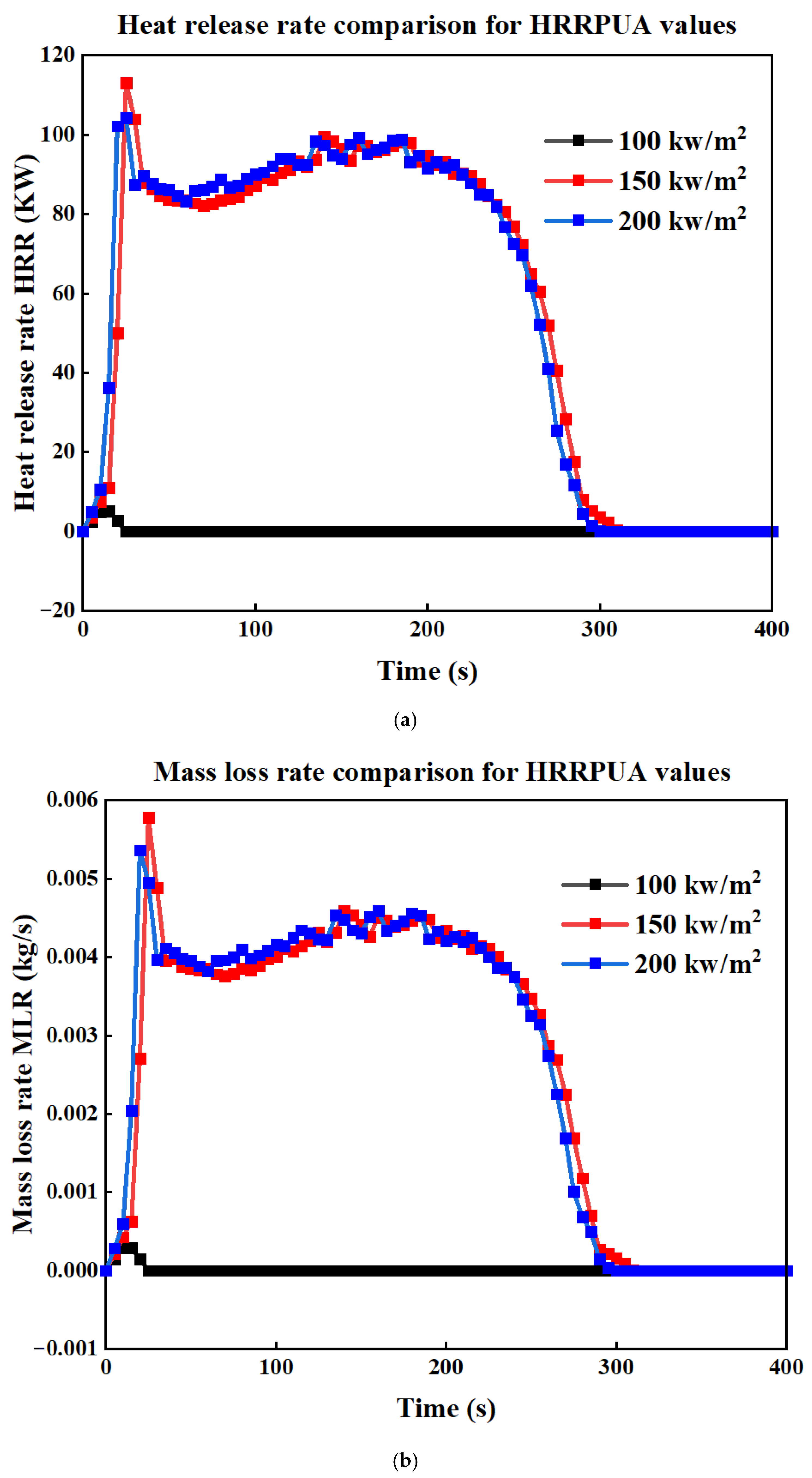
In this section, we discuss simulations using three different ignition line intensities (HRRPUA): 100 kW/m², 150 kW/m², and 200 kW/m². The results, presented in Figure A1, show that the 100 kW/m² intensity is insufficient to sustain surface fire propagation, as evidenced by the lack of significant HRR or MLR throughout the simulation period. Furthermore, the HRR and MLR results for the 150 kW/m² and 200 kW/m² cases display no substantial differences, indicating that both intensities yield similar outcomes. Based on these findings, we selected an HRRPUA of 150 kW/m² for our simulations.

Figure A1. (a) Comparison of HRR and (b) MLR for three cases with different HRRPUA values, for surface fire simulations.

Figure A1. (a) Comparison of HRR and (b) MLR for three cases with different HRRPUA values, for surface fire simulations.

Appendix A.1.2. Domain Size

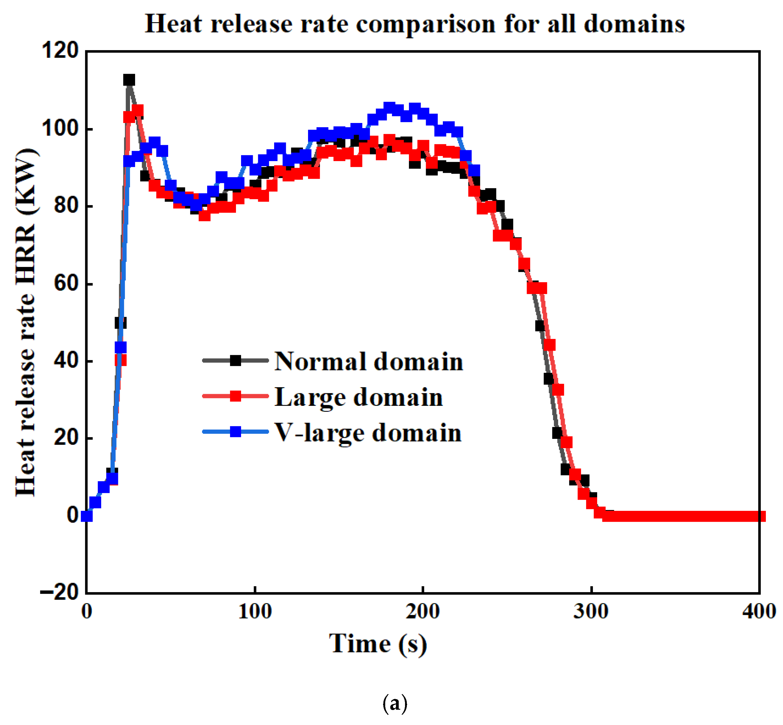
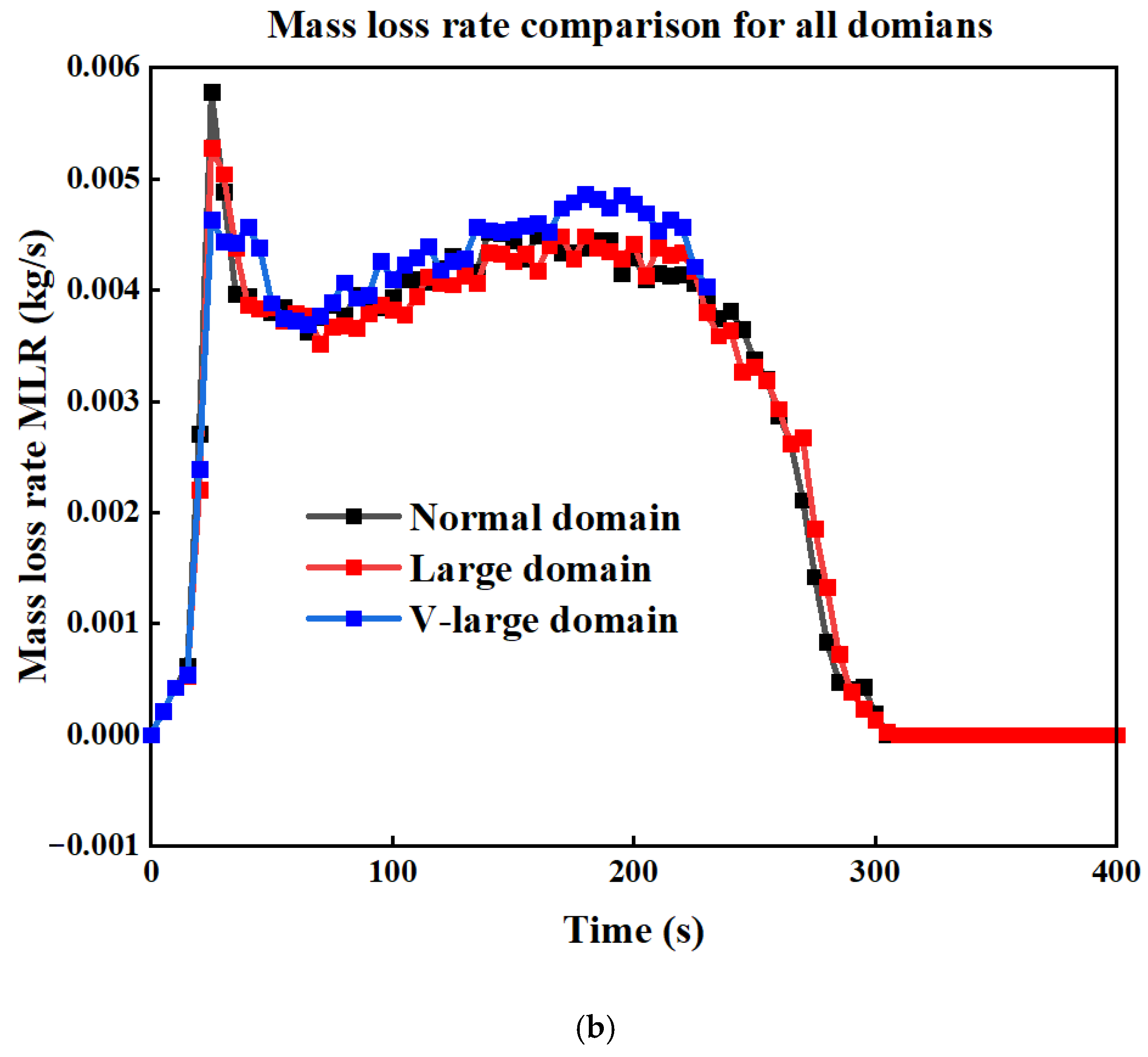
In this section, we conducted simulations using three domain sizes labelled as “normal,” “large,” and “very large,” as detailed in Table A1, which also provides the dimensions for each domain. This comparison aims to assess the impact of domain size on fire growth. The results, presented in Figure A2, illustrate the differences in the HRR and MLR across these cases. As shown in Figure A2a,b, there are no significant differences in the HRR and MLR between the normal and large domains. This finding suggests that the normal domain is the more efficient choice in terms of computational resources without affecting the accuracy.

Table A1. The dimensions of the simulated domains.

Simulation	Domain Size	Distance of Ignition Line from Inlet	Bordering Subdomain (Both Sides)	Distance from End of the Burnable Plot to the Outlet
V-large domain	8 m long × 4 m wide × 2.5 m high	3.25 m	1.5 m	3.25 m
Large domain	6 m long × 3m wide × 2 m high	2.25 m	1 m	2.25 m
Normal domain	4 m long × 2 m wide × 1.5 m high	1.25 m	0.5 m	1.25 m

Table A1. The dimensions of the simulated domains.

Simulation	Domain Size	Distance of Ignition Line from Inlet	Bordering Subdomain (Both Sides)	Distance from End of the Burnable Plot to the Outlet
V-large domain	8 m long × 4 m wide × 2.5 m high	3.25 m	1.5 m	3.25 m
Large domain	6 m long × 3m wide × 2 m high	2.25 m	1 m	2.25 m
Normal domain	4 m long × 2 m wide × 1.5 m high	1.25 m	0.5 m	1.25 m

Figure A2. (a) Comparison of HRR and (b) MLR for three cases with different domain sizes, for surface fire simulations.

Figure A2. (a) Comparison of HRR and (b) MLR for three cases with different domain sizes, for surface fire simulations.

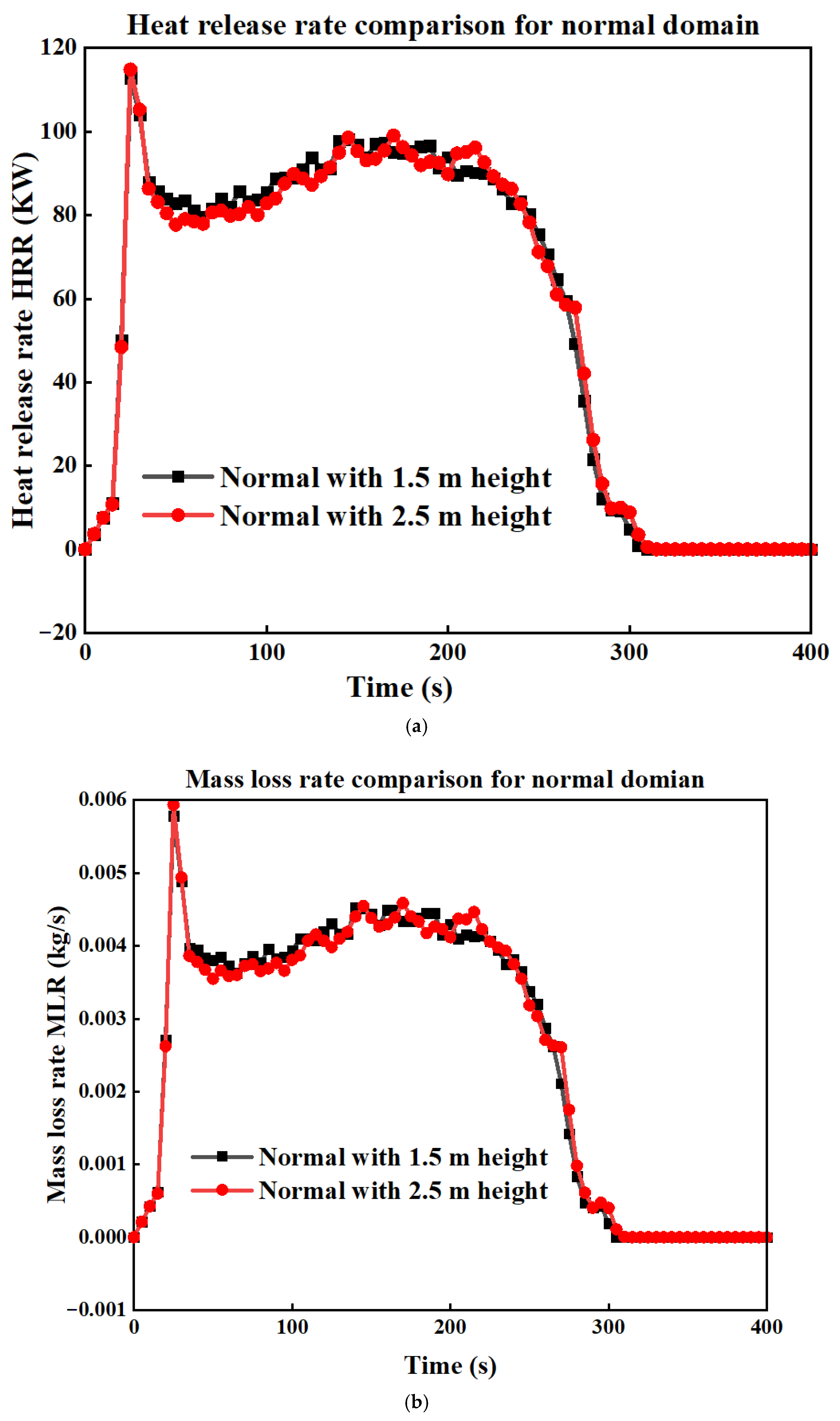
In our sensitivity analysis for a zero slope, a domain height of 1.5 m is sufficient without affecting the results. However, for slopes of 10° and 20°, especially using the step method, 1.5 m is not adequate due to the increased flame height. To resolve this, we compared the normal domain at heights of 1.5 m and 2.5 m. As shown in Figure A3, there is no significant difference in HRR and MLR between the two domains with different heights. Therefore, we will use the normal domain dimensions with a height of 2.5 m for our simulations.

Table A2 gives details about all the other simulated cases included in the surface fire simulations.

Table A2. Descriptions of all the simulated cases.

Case	Slope	Slope Method	Grid Size
Z1C	Zero	Non	1 cm
Z2C	Zero	Non	2 cm
S10G1C	10° slope	Gravity	1 cm
S10G2C	10° slope	Gravity	2 cm
S10S1C	10° slope	Step	1 cm
S10S2C	10° slope	Step	2 cm
S20G1C	20° slope	Gravity	1 cm
S20G2C	20° slope	Gravity	2 cm
S20S1C	20° slope	Step	1 cm
S20S2C	20° slope	Step	2 cm

Table A2. Descriptions of all the simulated cases.

Case	Slope	Slope Method	Grid Size
Z1C	Zero	Non	1 cm
Z2C	Zero	Non	2 cm
S10G1C	10° slope	Gravity	1 cm
S10G2C	10° slope	Gravity	2 cm
S10S1C	10° slope	Step	1 cm
S10S2C	10° slope	Step	2 cm
S20G1C	20° slope	Gravity	1 cm
S20G2C	20° slope	Gravity	2 cm
S20S1C	20° slope	Step	1 cm
S20S2C	20° slope	Step	2 cm

Figure A3. (a) Comparison of HRR and (b) MLR for the normal domain with two different domain heights.

Figure A3. (a) Comparison of HRR and (b) MLR for the normal domain with two different domain heights.

Appendix A.2. Single Douglas Fir Tree

We will conduct sensitivity analyses for the single Douglas fir tree on ignition line intensity and domain size, in addition to the grid size sensitivity analysis already conducted in Section 3.2.

Appendix A.2.1. Ignition Line Intensity (HRRPUA)

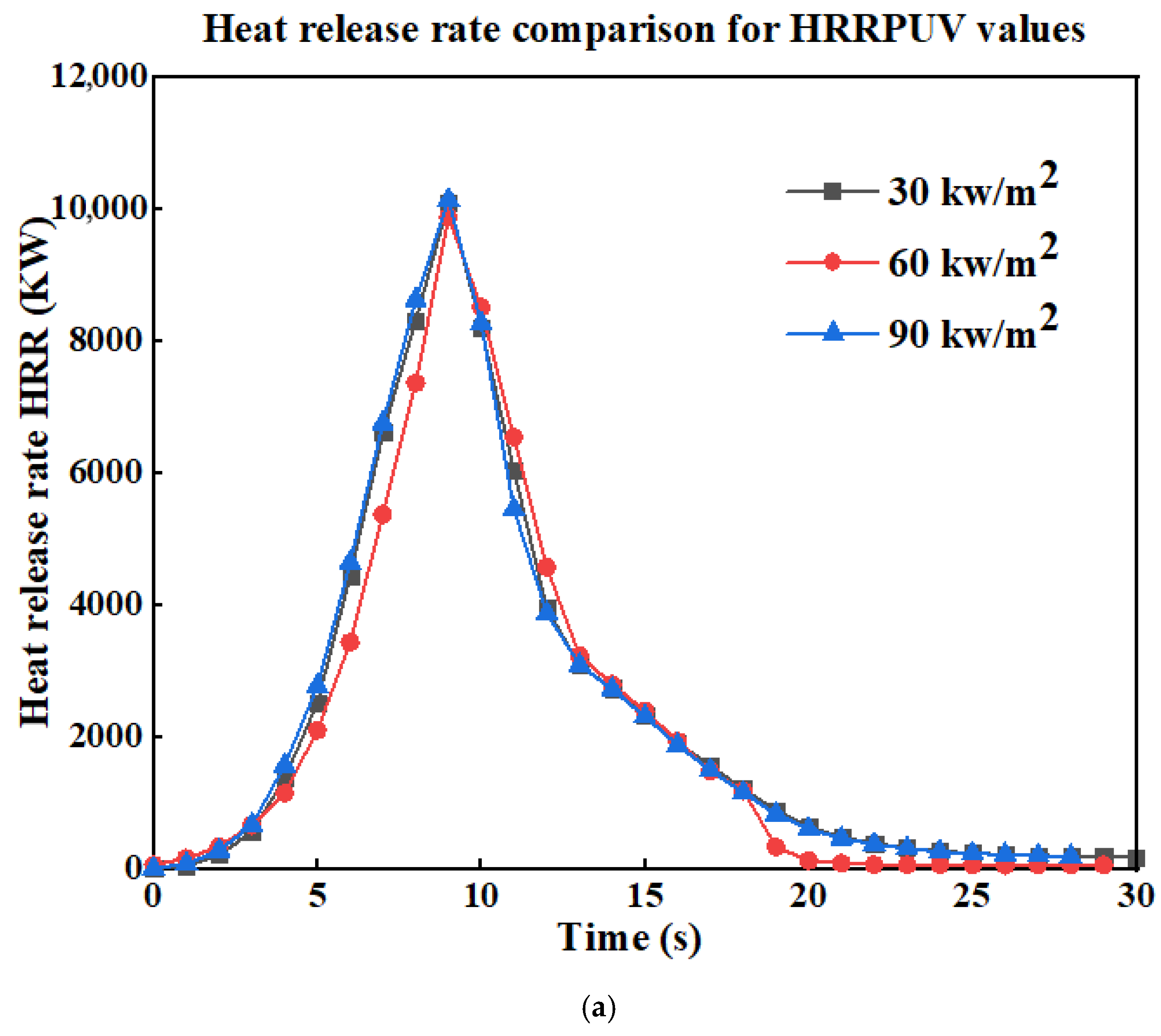
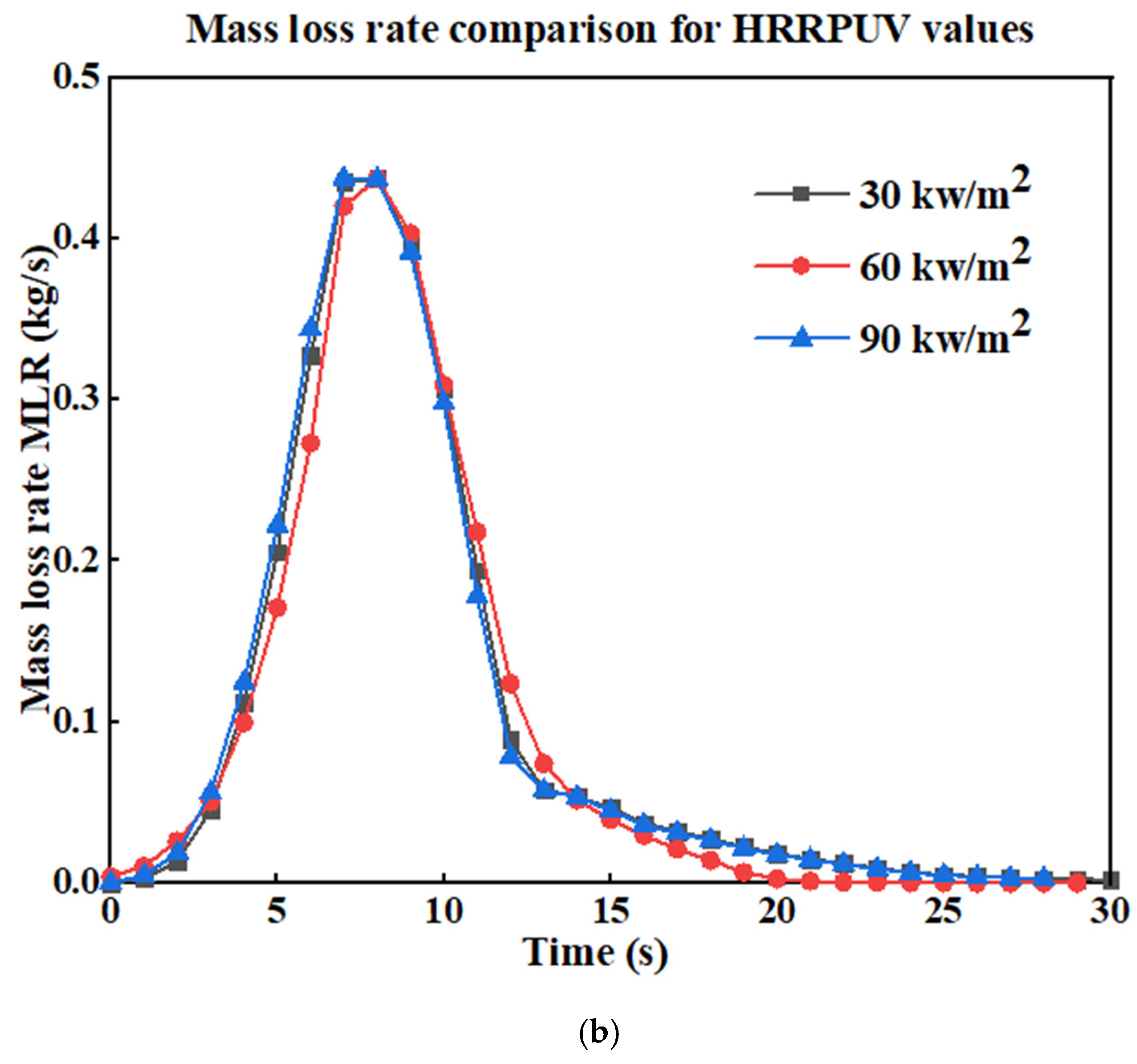
In this section, we apply the same methodology used in the surface fire simulations to assess the sensitivity of our results to different ignition line intensities (HRRPUA). We simulated three cases using HRRPUA values of 30 kW/m², 60 kW/m², and 90 kW/m². As shown in Figure A4, there are no significant differences in the HRR or MLR among the three cases. Therefore, we adopt the average value, 60 kW/m², which was also used in the original study conducted by Mell.

Figure A4. (a) Comparison of HRR and (b) MLR for three cases with different HRRPUA values for the single Douglas fir tree simulation.

Figure A4. (a) Comparison of HRR and (b) MLR for three cases with different HRRPUA values for the single Douglas fir tree simulation.

Appendix A.2.2. Domain Size

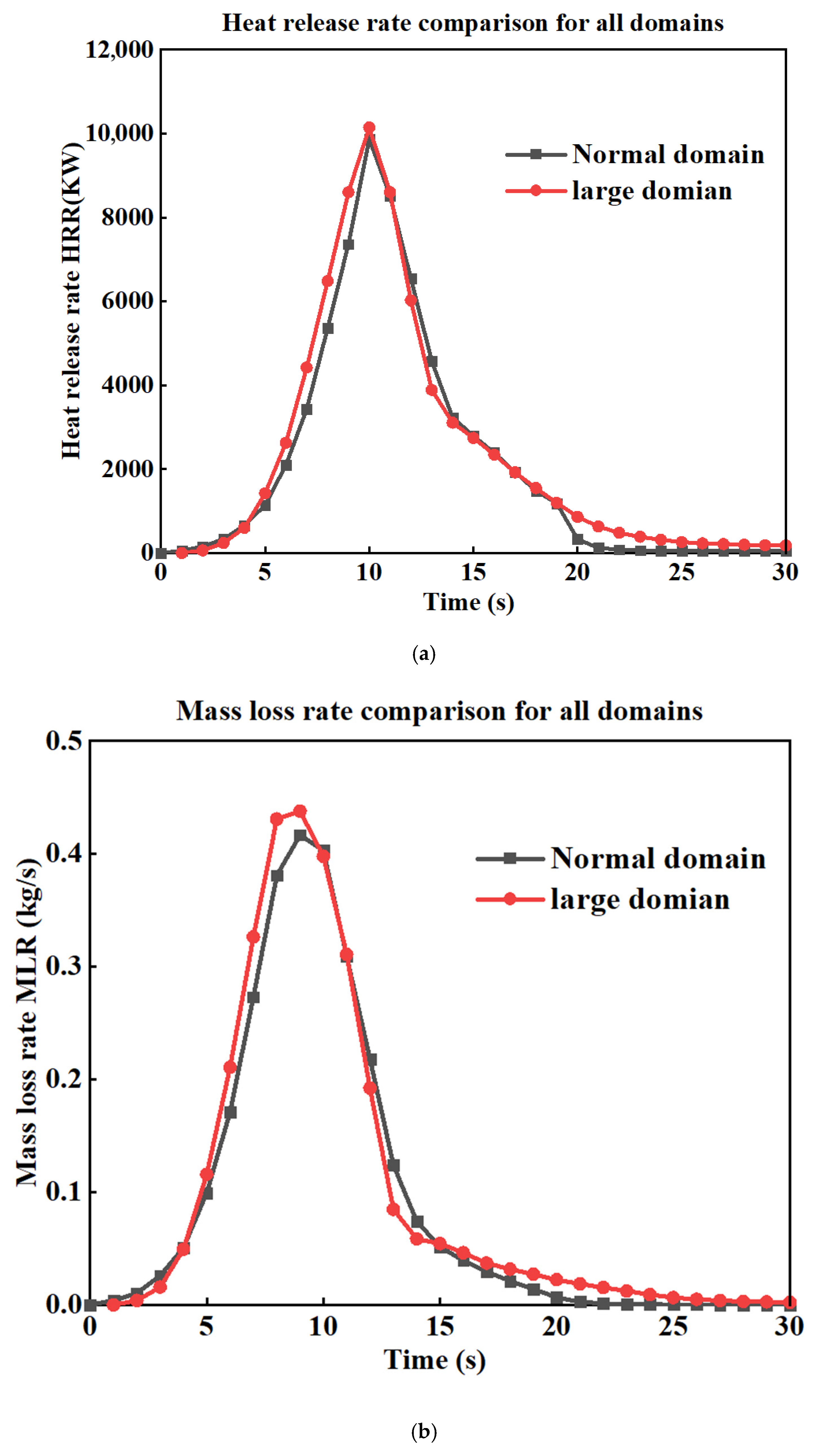
In this section, we adopt the same methodology used in the surface fire simulation to assess the sensitivity of our results to domain size. We compare the HRR shown in Figure 7a and the MLR shown in Figure A5b for two computational domains: a larger domain and the standard domain used throughout our simulations. We cannot adopt a smaller domain in this study, as it would not be sufficient to include both the tree and the heat flux sensors in their original positions, as presented in the experimental setup. The standard domain also corresponds to the one used in the original study by Mell. The dimensions of both domains are provided in Table A3. The comparison reveals no significant differences in the HRR or MLR between the large and standard domains. Therefore, we proceed with the standard (smaller) domain for the remainder of our simulations, as it offers a more computationally efficient option without compromising the accuracy of the results.

Table A3. The dimensions of the simulated domains for the single Douglas fir tree.

Simulation	Domain Size	Distance of Tree Centre from Inlet
Large domain	9.6 m long × 4.8 m wide × 9.6 m high	2.4 m
Normal domain	4.8 m long × 2.4 m wide × 9.6 m high	1.2 m

Table A3. The dimensions of the simulated domains for the single Douglas fir tree.

Simulation	Domain Size	Distance of Tree Centre from Inlet
Large domain	9.6 m long × 4.8 m wide × 9.6 m high	2.4 m
Normal domain	4.8 m long × 2.4 m wide × 9.6 m high	1.2 m

Figure A5. (a) Comparison of HRR and (b) MLR for two cases with different domain sizes, for the single Douglas fir tree simulation.

Figure A5. (a) Comparison of HRR and (b) MLR for two cases with different domain sizes, for the single Douglas fir tree simulation.

The input script utilized for single Douglas fir tree simulation can be found at the following location: fds/Validation/NIST_Douglas_Firs/FDS_Input_Files/tree_2_m_14_pc.fds at master·firemodels/fds·GitHub (https://github.com/firemodels/fds, accessed on 20 February 2025).

References

- Rein, G.; Huang, X. Smouldering wildfires in peatlands, forests and the arctic: Challenges and perspectives. Curr. Opin. Environ. Sci. Health 2021, 24, 100296. [Google Scholar] [CrossRef] [Scilit]
- Bennett, M.; Fitzgerald, S.A.; Parker, B.; Main, M.L.; Perleberg, A.; Schnepf, C.; Mahoney, R.L. Reducing Fire Risk on Your Forest Property. 2010. Available online: https://ir.library.oregonstate.edu/concern/administrative_report_or_publications/ws859f89n (accessed on 15 March 2025).
- Rothermel, R.C. Predicting Behavior and Size of Crown Fires in the Northern Rocky Mountains; US Department of Agriculture, Forest Service, Intermountain Research Station: Ogden, UT, USA, 1991.
- McArthur, A.G.; Forest Research Institute. Forest Fire Danger Meter; Forest Research Institute, Forestry & Timber Bureau: Canberra, Australia, 1973. [Google Scholar]
- Sullivan, A.; Knight, I. Estimating error in wind speed measurements for experimental fires. Can. J. For. Res. 2001, 31, 401–409. [Google Scholar] [CrossRef]
- Rothermel, R.C. How to Predict the Spread and Intensity of Forest and Range Fires; US Department of Agriculture, Forest Service, Intermountain Forest and Range: Ogden, UT, USA, 1983.
- Alexander, M.E.; Lawson, B.D.; Stocks, B.J.; Van Wagner, C.E. User Guide to the Canadian Forest Fire Behavior Prediction System: Rate of Spread Relationships; Canadian Forestry Service: Ottawa, ON, Canada, 1984. [Google Scholar]
- Gould, J.S.; McCaw, W.; Cheney, N.; Ellis, P.F.; Knight, I.; Sullivan, A.L. Project Vesta: Fire in Dry Eucalypt Forest: Fuel Structure, Fuel Dynamics and Fire Behaviour; Csiro Publishing: Clayton, VIC, Australia, 2008. [Google Scholar]
- Finney, M.A. FARSITE, Fire Area Simulator—Model Development and Evaluation; US Department of Agriculture, Forest Service, Rocky Mountain Research Station: Fort Collins, CO, USA, 1998; No. 4. [Google Scholar]
- Tolhurst, K.; Shields, B.; Chong, D. Phoenix: Development and application of a bushfire risk management tool. Aust. J. Emerg. Manag. 2008, 23, 47–54. [Google Scholar]
- Miller, C.; Hilton, J.; Sullivan, A.; Prakash, M. SPARK–A bushfire spread prediction tool. In International Symposium on Environmental Software Systems; Springer: Berlin/Heidelberg, Germany, 2015; pp. 262–271. [Google Scholar]
- Beer, T. The interaction of wind and fire. Bound.-Layer Meteorol. 1991, 54, 287–308. [Google Scholar] [CrossRef] [Scilit]
- Grishin, A.M. Mathematical Modeling of Forest Fires and New Methods of Fighting Them; Publishing House of the Tomsk State University: Tomsk, Russia, 1997. [Google Scholar]
- Larini, M.; Giroud, F.; Porterie, B.; Loraud, J.-C. A multiphase formulation for fire propagation in heterogeneous combustible media. Int. J. Heat Mass Transf. 1998, 41, 881–897. [Google Scholar] [CrossRef] [Scilit]
- Morvan, D. Physical phenomena and length scales governing the behaviour of wildfires: A case for physical modelling. Fire Technol. 2011, 47, 437–460. [Google Scholar] [CrossRef] [Scilit]
- Pastor, E.; Zárate, L.; Planas, E.; Arnaldos, J. Mathematical models and calculation systems for the study of wildland fire behaviour. Prog. Energy Combust. Sci. 2003, 29, 139–153. [Google Scholar] [CrossRef] [Scilit]
- Mell, W.; Jenkins, M.A.; Gould, J.; Cheney, P. A physics-based approach to modelling grassland fires. Int. J. Wildland Fire 2007, 16, 1–22. [Google Scholar] [CrossRef] [Scilit]
- Sullivan, A.L. Wildland surface fire spread modelling, 1990–2007. 1: Physical and quasi-physical models. Int. J. Wildland Fire 2009, 18, 349–368. [Google Scholar] [CrossRef] [Scilit]
- Mell, W.; Maranghides, A.; McDermott, R.; Manzello, S.L. Numerical simulation and experiments of burning douglas fir trees. Combust. Flame 2009, 156, 2023–2041. [Google Scholar] [CrossRef] [Scilit]
- Dahale, A.; Ferguson, S.; Shotorban, B.; Mahalingam, S. Effects of distribution of bulk density and moisture content on shrub fires. Int. J. Wildland Fire 2013, 22, 625–641. [Google Scholar] [CrossRef] [Scilit]
- Wadhwani, R.; Sutherland, D.; Moinuddin, K.; Huang, X. Numerical simulation of two parallel merging wildfires. Int. J. Wildland Fire 2023, 32, 1726–1740. [Google Scholar] [CrossRef] [Scilit]
- Mueller, E.V.; Campbell-Lochrie, Z.; Walker-Ravena, C.; Hadden, R.M. Numerical simulations of flame spread in pine needle beds using simple thermal decomposition models. Fire Saf. J. 2023, 141, 103886. [Google Scholar] [CrossRef] [Scilit]
- El Houssami, M.; Lamorlette, A.; Morvan, D.; Hadden, R.M.; Simeoni, A. Framework for submodel improvement in wildfire modeling. Combust. Flame 2018, 190, 12–24. [Google Scholar] [CrossRef] [Scilit]
- Korobeinichev, O.; Kumaran, S.M.; Raghavan, V.; Trubachev, S.; Paletsky, A.; Shmakov, A.; Glaznev, R.; Chernov, A.; Tereshchenko, A.; Loboda, E. Investigation of the impact of pinus silvestris pine needles bed parameters on the spread of ground fire in still air. Combust. Sci. Technol. 2023, 195, 3072–3094. [Google Scholar] [CrossRef] [Scilit]
- Korobeinichev, O.; Kumaran, S.M.; Shanmugasundaram, D.; Raghavan, V.; Trubachev, S.; Paletsky, A.; Shmakov, A.; Glaznev, R.; Chernov, A.; Tereshchenko, A. Experimental and numerical study of flame spread over bed of pine needles. Fire Technol. 2022, 58, 1227–1264. [Google Scholar] [CrossRef] [Scilit]
- Morvan, D.; Accary, G.; Meradji, S.; Frangieh, N.; Bessonov, O. A 3D physical model to study the behavior of vegetation fires at laboratory scale. Fire Saf. J. 2018, 101, 39–52. [Google Scholar] [CrossRef] [Scilit]
- Perez-Ramirez, Y.; Mell, W.E.; Santoni, P.-A.; Tramoni, J.-B.; Bosseur, F. Examination of WFDS in modeling spreading fires in a furniture calorimeter. Fire Technol. 2017, 53, 1795–1832. [Google Scholar] [CrossRef] [Scilit]
- Mueller, E.V.; Skowronski, N.S.; Clark, K.L.; Gallagher, M.R.; Mell, W.E.; Simeoni, A.; Hadden, R.M. Detailed physical modeling of wildland fire dynamics at field scale-An experimentally informed evaluation. Fire Saf. J. 2021, 120, 103051. [Google Scholar] [CrossRef] [Scilit]
- Moinuddin, K.A.M.; Sutherland, D.; Mell, W. Simulation study of grass fire using a physics-based model: Striving towards numerical rigour and the effect of grass height on the rate of spread. Int. J. Wildland Fire 2018, 27, 800–814. [Google Scholar] [CrossRef] [Scilit]
- McGrattan, K.; Klein, B.; Hostikka, S.; Floyd, J. Fire Dynamics Simulator (Version 5), User’s Guide; NIST Special Publication: Gaithersburg, MD, USA, 2010; Volume 1019, No. 5, pp. 1–186. [Google Scholar]
- McGrattan, K.; Hostikka, S.; Floyd, J.; Baum, H.; Rehm, R.; Mell, W.; McDermott, R. Fire Dynamics Simulator (Version 5) Technical Reference Guide; NIST Special Publication: Gaithersburg, MD, USA, 2010; Volume 1018, No. 5. [Google Scholar]
- Miloua, H. Numerical prediction of the fire spread in vegetative fuels using NISTWFDS Model. Int. J. Eng. Res. Afr. 2016, 20, 177–192. [Google Scholar] [CrossRef] [Scilit]
- Innocent, J.; Sutherland, D.; Khan, N.; Moinuddin, K. Physics-based simulations of grassfire propagation on sloped terrain at field scale: Motivations, model reliability, rate of spread and fire intensity. Int. J. Wildland Fire 2023, 32, 496–512. [Google Scholar] [CrossRef] [Scilit]
- Yang, Z.; Zhang, H.; Zhang, L.; Chen, H. Experimental Study on Downslope Fire Spread over a Pine Needle Fuel Bed. Fire Technol. 2018, 54, 1487–1503. [Google Scholar] [CrossRef] [Scilit]
- Ribeiro, C.; Reis, L.; Raposo, J.; Rodrigues, A.; Viegas, D.X.; Sharples, J. Interaction between two parallel fire fronts under different wind conditions. Int. J. Wildland Fire 2022, 31, 492–506. [Google Scholar] [CrossRef] [Scilit]
- Gupta, S.; Sharaf, M.; Arun, M.; Guerrierri, M.; Moinuddin, K. Experimental and Numerical Investigation of Burning Characteristics of Australian Pine Trees for Wildfire Modelling Combustion and Flame. Fire Saf. J. 2025, 157, 104500. [Google Scholar] [CrossRef] [Scilit]
- McGrattan, K. (Ed.) Fire Dynamics Simulator (Version 4) Technical Reference Guide; N.S.P. 1018; NIST: Gaithersburg, MD, USA, 2006. [Google Scholar]
- Abu-Bakar, A.S. Characterization of Fire Properties for Coupled Pyrolysis and Combustion Simulation and Their Optimised Use. Ph.D. Thesis, Victoria University, Melbourne, VIC, Australia, 2015. [Google Scholar]
- McGrattan, K.; Klein, B.; Hostikka, S.; Floyd, J. Fire Dynamics Simulator (Version 5), User’s Guide; NIST Special Publication: Gaithersburg, MD, USA, 2008; Volume 1019, No. 6. [Google Scholar]
- Kling, T.; Korhonen, T.; Verma, N.; Hakkarainen, T.; Maijala, T.; Gorshkova, E.; Niemi, T.; Kallio, S. D5.4_FIRE-RES_Modelling-of-Fire-Combustion-and-Convective-Processes_Compressed; VTT Technical Research Centre of Finland Ltd.: Espoo, Finland, 2024. [Google Scholar]
- Soummar, A.; Miloua, H. Using the CFD capabilities of FDS to predict a vegetation fire in a sloped terrain. Ukr. J. Ecol. 2022, 12, 47–56. [Google Scholar]
- Sánchez-Monroy, X.; Mell, W.; Torres-Arenas, J.; Butler, B. Fire spread upslope: Numerical simulation of laboratory experiments. Fire Saf. J. 2019, 108, 102844. [Google Scholar] [CrossRef] [Scilit]
- Peduzzi, E.; Boissonnet, G.; Maréchal, F. Biomass modelling: Estimating thermodynamic properties from the elemental composition. Fuel 2016, 181, 207–217. [Google Scholar] [CrossRef] [Scilit]
- Jayalakshmy, M.S.; Philip, J. Thermophysical Properties of Plant Leaves and Their Influence on the Environment Temperature. Int. J. Thermophys. 2010, 31, 2295–2304. [Google Scholar] [CrossRef] [Scilit]
- Amini, E.; Safdari, M.-S.; Johnson, N.; Weise, D.R.; Fletcher, T.H. Pyrolysis kinetics of wildland vegetation using model-fitting methods. J. Anal. Appl. Pyrolysis 2021, 157, 105167. [Google Scholar] [CrossRef] [Scilit]
- Lautenberger, C.; Fernandez-Pello, C. Optimization algorithms for material pyrolysis property estimation. Fire Saf. Sci. 2011, 10, 459–470. [Google Scholar] [CrossRef]
- Wei, S.; Liu, F.; Chen, X.; Huang, G.; Li, C.; Ding, Y. Thermal degradation behavior of Photinia × fraseri Dress leaves based on TG-FTIR and main components separation by SCE optimization. Biomass Convers. Biorefinery 2024, 15, 16473–16483. [Google Scholar] [CrossRef] [Scilit]
- Roy, C.J. Grid convergence error analysis for mixed-order numerical schemes. AIAA J. 2003, 41, 595–604. [Google Scholar] [CrossRef] [Scilit]
- Cobian-Iñiguez, J.; Aminfar, A.; Weise, D.R.; Princevac, M. On the use of semi-empirical flame models for spreading chaparral crown fire. Front. Mech. Eng. 2019, 5, 50. [Google Scholar] [CrossRef] [Scilit]
- Montakhab, A.A. Numerical Investigation of the Effect of Inlet Turbulence Intensity on a Bluff-Body Stabilized Flame at Near Blow-Off Condition; Syracuse University: Syracuse, NY, USA, 2022. [Google Scholar]
- Spalart, P. Strategies for turbulence modelling and simulations. In Engineering Turbulence Modelling and Experiments 4; Elsevier: Amsterdam, The Netherlands, 1999; pp. 3–17. [Google Scholar] [CrossRef] [Scilit]
- Morvan, D.; Frangieh, N. Wildland fires behaviour: Wind effect versus Byram’s convective number and consequences upon the regime of propagation. Int. J. Wildland Fire 2018, 27, 636–641. [Google Scholar] [CrossRef] [Scilit]
Disclaimer/Publisher’s Note: The statements, opinions and data contained in all publications are solely those of the individual author(s) and contributor(s) and not of MDPI and/or the editor(s). MDPI and/or the editor(s) disclaim responsibility for any injury to people or property resulting from any ideas, methods, instructions or products referred to in the content. |
© 2026 by the authors. Licensee MDPI, Basel, Switzerland. This article is an open access article distributed under the terms and conditions of the Creative Commons Attribution (CC BY) license.