Rational (a, p)−Quasicontractions and Fractional Delayed Nonlocal Caputo Problems via Hammerstein Operators

Abstract

We introduce and study a new class of nonlinear operators on metric spaces, called rational $(a,p)-$quasicontractions. Within this framework, we establish Greguš-type fixed-point theorems for closed, convex subsets of Banach spaces. The results establish the existence and uniqueness of fixed points, as well as the convergence of the Picard iteration for every initial guess. We show that rational $(a,p)-$quasicontractions strictly extend several classical contractive classes, including Hardy-Rogers, Kannan, Chatterjea, and rational contractions, and we provide explicit examples exhibiting the properness of these inclusions. As an application, we consider a nonlocal boundary value problem for a Caputo fractional differential equation of order $\alpha \in (1,2)$ with distributed delay and mixed nonlocal boundary conditions. By rewriting the problem as a Hammerstein-Volterra integral equation on a cone, and imposing natural growth and rational Lipschitz conditions on the delayed nonlinearity, we show that the associated Hammerstein operator is a rational $(a,p)-$quasicontraction. This yields the existence, uniqueness, and global attractivity of a positive solution. Two model fractional nonlinearities with delayed feedback are discussed in detail, along with a numerical scheme that illustrates the predicted geometric convergence of the discrete Picard iteration in the Caputo fractional setting.

1. Introduction

Fixed point theory in metric spaces is one of the most influential ideas in modern mathematics. It started with Banach’s contraction principle [1], which shows that a simple contractive mapping on a complete metric space always admits a unique fixed point, and that successive approximations converge to it. Since then, many authors have extended this principle in different directions, including the well-known results of Kannan [2], Chatterjea [3], Hardy-Rogers [4], Edelstein [5], Meir-Keeler [6] and Greguš [7], each of which relaxes or modifies the contraction condition in a distinctive way. These generalizations have created a rich framework in which abstract convergence arguments meet concrete applications, especially in the study of nonlinear differential and integral equations, boundary value problems, and iterative methods in applied mathematics.

Among the more recent developments, Popescu and Stan [8,9] introduced $(a,p)-$quasicontractions, including the quadratic case $p=2$, where the interpoint distance and self-deviation terms are balanced at the $p-$power level. In many operator-theoretic models, however, particularly those arising from Hammerstein-type formulations of boundary value problems, the interpoint block $d^p(x,y)$ may become large on relevant invariant sets, and this can destroy the effective contractive behaviour needed for robust global iteration schemes.

Fixed point theory has become a standard tool for establishing existence-uniqueness, convergence, and Ulam-Hyers type stability results across a broad spectrum of nonlinear models, especially in fractional and nonlocal problems. Recent works illustrate this role for Caputo-type nonlinear fractional differential equations and their Ulam-Hyers stability [10], dynamic programming and fractional equations in partial modular $b-$metric spaces [11], and fourth-order boundary value problems [12]. Further applications include Ulam stability for variable-order $\phi -$Hilfer fractional implicit integro-differential equations [13], fractional-order delay differential equations [14], coupled systems involving generalized proportional Caputo derivatives [15], and two-dimensional nonlocal fractional parabolic initial boundary value problems [16].

The present paper introduces a bounded-rational normalisation of the interpoint term in Equations (1) and (2), that is

$$d^p(x,y)⟼{\varphi }_p\left(d(x,y)\right):={\displaystyle \frac{d^p(x,y)}{1+d^p(x,y)}},p\in \mathbb{N}.$$

This transformation yields rational $(a,p)-$quasicontractions, which are within the $(a,p)-$framework because ${\varphi }_p\left(t\right)\le t^p$; however, they are structurally different from the rational extensions of Banach’s principle proposed earlier by Dass-Gupta and Jaggi, and are incomparable with Hardy-Rogers operators. The boundedness $0\le {\varphi }_p\left(t\right)<1$ for all $t\ge 0$ is the key feature that allows us to obtain explicit admissible ranges for a and global Lipschitz constants that depend only on $(a,p)$. This simple modification yields contractive inequalities in which the interpoint contribution is uniformly bounded, making the theory particularly well suited to operators whose natural phase space has a large diameter.

Our first group of results consists of fixed-point theorems for rational $(a,p)-$quasicont- ractions. On compact metric spaces, we prove that a rational $(a,p)-$quasicontraction has a unique fixed point, and the Picard iteration converges to it from every starting point. On closed, convex subsets of Banach spaces, we obtain analogous results under a sequential continuity assumption. Several examples on $[-1,1]$ demonstrate that the rational classes may fail all Hardy-Rogers inequalities, confirming that the rational framework strictly extends the classical linear theory.

We apply the abstract theory to a delayed multi-point Caputo fractional boundary value problem with nonlocal conditions. By rewriting the problem as a Hammerstein-Volterra integral equation and deriving two-sided bounds for the associated Green kernel, we construct an invariant cone-ball and prove that the resulting operator is a strict rational $(a,p)-$quasicontraction with relatively compact range. This yields existence, uniqueness, and global attractivity of a positive solution. Finally, we present a collocation-based discretisation of the Hammerstein equation and illustrate the predicted geometrically fast convergence of the discrete Picard iteration. Fractional models with memory and delay naturally lead to nonlinear Hammerstein-type operators whose contractive behaviour may be destroyed by large interpoint distances in the underlying phase space. The bounded rational $(a,p)-$framework developed here is therefore particularly well-suited for fractional and delayed problems, such as the Caputo-type boundary value problem treated in Section 4.

The paper is organised as follows. Section 2 collects the preliminary notation and recalls the $(a,p)-$framework in the sense of Popescu-Stan, together with basic properties of the rational normalisation ${\varphi }_p$. Section 3 introduces the rational classes and proves the main fixed-point theorems. Section 4 treats the delayed nonlocal Caputo problem via a Hammerstein-Volterra operator and provides numerical illustrations. Section 5 contains the conclusions and perspectives.

2. Preliminaries

More recently, Popescu and Stan [8,9] introduced quadratic and $(a,p)-$quasicontractions, which blend interpoint distances with self deviation terms at the $p-$power level, yielding strong fixed point results in compact and Banach settings.

Definition 1

([8]). A mapping $T:X\to X$ of a metric space $(X,d)$ to itself is said to be a $(a,p)-$quasicontraction if there exists $a\in (0,\frac{1}{2})$ and $p\in \mathbb{N}$ such that

$$d^p(Tu,Tv)\le a{d}^p(u,Tu)+a{d}^p(v,Tv)+(1-2a)d^p(u,v)$$

(1)

for all $u,v\in X$. We say that T is a strict $(a,p)-$quasicontraction if in Equation (1) the inequality is strict for all $u,v\in X$ with $u\ne v$.

Indeed, this concept is a generalization of the idea presented by Popescu and Stan [9] by taking $p=2$, which is also defined as follows.

Remark 1

([9]). A mapping $T:X\to X$ of a metric space $(X,d)$ into itself is a quadratic quasicontraction if there exists $a\in (0,\frac{1}{2})$ such that

$$d^2(Tx,Ty)\le a{d}^2(x,Tx)+a{d}^2(y,Ty)+(1-2a)d^2(x,y)$$

(2)

for all $x,y\in X$. In addition, T is a strict quadratic quasicontraction if in Equation (2) we have a strict inequality for all $x,y\in X$ with $x\ne y$.

The conceptual framework surrounding fixed point theorems has undergone considerable advancement since the seminal contributions of Banach [1]. Subsequent generalizations have been developed by a number of prominent scholars, including Edelstein [5], Meir and Keeler [6], Hardy and Rogers [4], and Greguš [7]. Correspondingly, rational-type extensions were introduced by Das and Gupta [17] and Jaggi [18]. Das and Gupta considered inequalities of the form

$$d(Tx,Ty)\le \alpha {\displaystyle \frac{d(y,Ty)(1+d(x,Tx\left)\right)}{1+d(x,y)}}+\beta d(x,y),$$

whereas Jaggi proposed

$$d(Tx,Ty)\le \alpha {\displaystyle \frac{d(x,Tx)d(y,Ty)}{d(x,y)}}+\beta d(x,y),$$

both under the condition $\alpha ,\beta \ge 0$ with $\alpha +\beta <1$. These forms are rational in nature but still rely on unbounded dependence on $d(x,y)$. By contrast, the investigation into quadratic and $(a,p)-$quasicontractions, as delineated by Popescu and Stan [8,9], reveal a more direct interplay between interpoint and self-deviation terms at the $p-$power level. This motivates the bounded rational normalization introduced in the present work, where $d^p(x,y)$ is replaced by $\frac{d^p(x,y)}{1+d^p(x,y)}$.

Throughout the paper:

• $(X,d)$ denotes a metric space, and $C\subseteq X$ is a nonempty subset assumed compact, closed, and convex as specified in each theorem.
• $p\in \mathbb{N}$ and $a\in (0,\frac{1}{2})$ are fixed parameters of the quasicontractive inequalities.
• For $x,y\in X$, we write $d^p(x,y):={\left(d(x,y)\right)}^p$.
• Inequalities of the form $d^p(Tx,Ty)\le \cdots$ are called strict if they hold with < whenever $x\ne y$.
• ${\varphi }_p:[0,\infty )\to [0,1)$ is the rational normalization

  $${\varphi }_p\left(t\right):={\displaystyle \frac{t^p}{1+t^p}}(t\ge 0).$$
• For a self-map $T:X\to X$, $T^n$ denotes the $n-$fold iterate ($T^0=\mathrm{Id}$), and the Picard sequence is $x_{n+1}=T{x}_n$.
• For $t\ge 0$, one has

  $$0\le {\displaystyle \frac{t}{1+t}}\le t,{\displaystyle \frac{t}{1+t}}\mathrm{is}\mathrm{nondecreasing}\mathrm{in}t.$$

  (3)

The goal of the next section is to replace the unbounded interpoint term $d^p(u,v)$ in Equation (1) by its bounded rational counterpart ${\varphi }_p\left(d(u,v)\right)$, and to develop fixed point theorems and quantitative admissibility bounds in this rationally normalised setting.

3. Rational (a, p)−Quasicontractions and Some Fixed Point Results

The landscape of contraction mappings may be viewed in terms of their structural relations. At the core are the classical $(a,p)-$quasicontractions, which extend Banach’s principle by balancing interpoint and self-deviation terms at the $p-$power level. Our rational normalization modifies this framework by replacing the unbounded interpoint block $d^p(x,y)$ with its bounded variant $\frac{d^p(x,y)}{1+d^p(x,y)}$, thereby producing both a rational $(a,p)-$class and, in the case $p=2$, a rational quadratic variant. These classes are strictly contained in the $(a,p)-$framework since $\frac{t}{1+t}\le t$, yet remain incomparable with Hardy-Rogers type conditions.

Building upon the foundational research presented by Popescu et al. in their works [8,9], we have devised a novel contraction that incorporates rational terms.

Definition 2.

Let $(X,d)$ be a metric space, $p\in \mathbb{N}$ and $a\in (0,\frac{1}{2})$. For all $x,y\in X$, a self-mapping $T:X\to X$ is called a rational $(a,p)-$quasicontraction if the following inequality holds

$$d^p(Tx,Ty)\le a{d}^p(x,Tx)+a{d}^p(y,Ty)+(1-2a){\displaystyle \frac{d^p(x,y)}{1+d^p(x,y)}}.$$

(4)

In the case where the inequality holds strictly for $x\ne y$, it is concluded that T qualifies as a strict rational $(a,p)-$quasicontraction.

Remark 2.

In Equation (4) if p equals 2 as

$$d^2(Tx,Ty)\le a{d}^2(x,Tx)+a{d}^2(y,Ty)+(1-2a){\displaystyle \frac{d^2(x,y)}{1+d^2(x,y)}},$$

(5)

then the self-mapping T is called a rational $a-$quadratic quasicontraction, and the strictness condition is also valid.

Remark 3.

By Equation (3), the inequality Equation (4) implies the $(a,p)-$quasi contraction presented in [8] and for $p=2$ quadratic quasi contraction presented in [9]

$$d^p(Tx,Ty)\le a\left(d^p(x,Tx)+d^p(y,Ty)\right)+(1-2a)d^p(x,y).$$

(6)

Lemma 1.

If the self-mapping T, defined on a metric space $(X,d)$, satisfies Equation (4), then for every $x\in X$, we have

$$d(Tx,T^{2}x)\le d(x,Tx).$$

Proof. 

Apply Equation (4) with $y:=Tx$. If we use the subsequent expression

$${\displaystyle \frac{d^p(x,Tx)}{1+d^p(x,Tx)}}\le d^p(x,Tx)$$

considering the statement Equation (3) and $a\in (0,\frac{1}{2})$, we get $d^p(Tx,T^{2}x)\le d^p(x,Tx)$, hence the claim is concluded. □

Remark 4.

The rational $(a,p)-$quasicontractions given in Equation (4) differ from both Das-Gupta and Jaggi schemes in several structural aspects.

1. 

In both Das-Gupta and Jaggi forms, the right-hand side contains terms that grow at least linearly in $d(x,y)$ whenever $d(y,Ty)$ or $d(x,Tx)$ is nonzero. By contrast, our rational normalisation replaces $d^p(x,y)$ by the bounded quantity

$${\varphi }_p\left(d(x,y)\right):={\displaystyle \frac{d^p(x,y)}{1+d^p(x,y)}}\in [0,1),$$

so the “pure” interpoint contribution is uniformly bounded, regardless of the diameter of the underlying metric space.

2. 

The Das-Gupta inequality is asymmetric in the variables $(x,y)$ and mixes the self-deviation of y with the interpoint distance through the fraction ${\displaystyle \frac{d(y,Ty)\left(1+d(x,Tx)\right)}{1+d(x,y)}}$; Jaggi’s condition introduces a product term ${\displaystyle \frac{d(x,Tx)d(y,Ty)}{d(x,y)}}$, which becomes singular as $d(x,y)\to 0$ and requires additional side conditions. In Equation (4), the self-deviation block $d^p(x,Tx)+d^p(y,Ty)$ and the interpoint block ${\varphi }_p\left(d(x,y)\right)$ appear separately and in a symmetric way, without singular behaviour at $x=y$.

3. 

The Das-Gupta and Jaggi classes involve two parameters $\alpha ,\beta$ constrained by $\alpha +\beta <1$, and in applications, one typically has to impose further operator-dependent restrictions on these constants. Our framework uses a single structural parameter $a\in (0,\frac{1}{2})$, and this makes the rational $(a,p)-$classes particularly convenient for operators arising from Hammerstein and Caputo problems, where one aims at explicit, model-independent contractivity bounds.

In summary, while all three schemes are “rational” in spirit, the bounded and symmetric normalisation of the interpoint term in our approach leads to a cleaner structure and enables the universal admissibility analysis developed later in the paper. A full set-theoretic comparison, inclusion or non-inclusion between the Das-Gupta, Jaggi, and rational $(a,p)-$classes would require a separate and rather technical study, and is therefore left for future work.

The novelty of our bounded rational framework can be summarized as follows:

i.

The replacement $d^p(x,y)\mapsto \frac{d^p(x,y)}{1+d^p(x,y)}$ enforces stronger contractivity and avoids the unbounded growth inherent in quadratic and $(a,p)-$schemes.

ii.

The approach yields explicit admissible constants, for instance, $a<1/6$ for the Hammerstein operator, and permits sharp separation results from Hardy-Rogers and related classes.

iii.

Unlike Das-Gupta and Jaggi’s rational forms, which introduce product fractions and auxiliary admissibility conditions, our scheme modifies only the interpoint block. This makes it structurally cleaner and more readily applicable in Banach and operator-theoretic settings.

Fixed Point Theorems in the Rational Framework

We now formulate robust fixed point theorems by leveraging the concepts of rational $(a,p)-$quasicontractions. This effort aims to enrich the theoretical framework of fixed point theory, offering fresh perspectives and enhancing the methodologies within this domain. By integrating these sophisticated quasicontractions, we aim to deepen our understanding of fixed-point phenomena and their applications across various mathematical settings.

Theorem 1.

Let $(X,d)$ represent a metric space, and $C\subset X$ denote a compact subset. If a mapping $T:C\to C$ is classified as a rational $(a,p)$ quasicontraction, it follows that T possesses a unique fixed point v within the set C. Moreover, the Picard iteration $x_{n+1}:=T{x}_n$ converges to $v\in C$ for every $x_0\in C$.

Proof. 

Initially, construct

$$\Pi :=inf\left\{d\right(x,Tx):x\in C\}$$

(7)

Considering the compactness property, we choose $\left(x_n\right)\subset C$ with $d(x_n,T{x}_n)\downarrow \Pi$, and after passing to subsequences, we have for all $u,v\in C$

$$x_n\to u,T{x}_n\to v,$$

which implies

$$d(u,v)=\underset{n\to \infty }{lim}d(x_n,T{x}_n)=\Pi .$$

(8)

In Equation (4), put the pair $(x_n,v)$ in place of $(x,y)$, and subsequently take the limit as n tends to infinity. This yields the following statement:

$$\begin{gathered} d^p(T{x}_n,Tv)\le a{d}^p(x_n,T{x}_n)+a{d}^p(v,Tv)+(1-2a){\displaystyle \frac{d^p(x_n,v)}{1+d^p(x_n,v)}} \\ {d}^p(v,Tv)\le a{\Pi }^p+a{d}^p(v,Tv)+(1-2a){\displaystyle \frac{{\Pi }^p}{1+{\Pi }^p}}. \end{gathered}$$

(9)

From Equation (9), we conclude that

$$(1-a)d^p(v,Tv)\le \left(a+{\displaystyle \frac{1-2a}{1+{\Pi }^p}}\right){\Pi }^p={\displaystyle \frac{(1-a){\Pi }^p+a{\Pi }^{2p}}{1+{\Pi }^p}}=(1-a){\Pi }^p-{\displaystyle \frac{(1-2a){\Pi }^{2p}}{1+{\Pi }^p}}.$$

Hence, this provides

$$(1-a)d^p(v,Tv)\le (1-a){\Pi }^p-{\displaystyle \frac{(1-2a){\Pi }^{2p}}{1+{\Pi }^p}}.$$

If $\Pi >0$ then the right-hand side is strictly smaller than $(1-a){\Pi }^p$, as $1-2a>0$, so $d^p(v,Tv)<{\Pi }^p$, which contradicts the definition of $\Pi$. Therefore, $\Pi =0$ and $d(v,Tv)=0$, which means that $v=Tv$ is a fixed point of T.

To prove the uniqueness of the fixed point, presume that $w\in X$ is another fixed point of the mapping $T.$ In Equation (4) employing $(x,y)=(v,w)$ yields

$$d^p(v,w)\le (1-2a){\displaystyle \frac{d^p(v,w)}{1+d^p(v,w)}}<d^p(v,w),$$

which is impossible unless $d(v,w)=0$. Hence $v=w$.

To obtain the convergence of the Picard iteration, let $x_{n+1}:=T{x}_n$ and set $u_n:=d^p(x_n,x_{n-1})$ for $n\ge 1$. In Equation (4), take $(x,y)=(x_n,x_{n-1})$; then, we have

$$u_{n+1}\le a{u}_n+a{u}_{n+1}+(1-2a){\displaystyle \frac{u_n}{1+u_n}}.$$

Hence,

$$(1-a)u_{n+1}\le a{u}_n+(1-2a){\displaystyle \frac{u_n}{1+u_n}}\le (1-a)u_n.$$

(10)

Thus, $\left(u_n\right)$ is a nonincreasing sequence and hence converges to some $r\ge 0$. Assume, by contradiction, that $r>0$. Apply Equation (4) to the pair $(x,y)=(x_n,x_{n+1})$. Since $T{x}_n=x_{n+1}$ and $T{x}_{n+1}=x_{n+2}$, we get

$$u_{n+2}=d^p(T{x}_n,T{x}_{n+1})\le a\left(d^p(x_n,T{x}_n)+d^p(x_{n+1},T{x}_{n+1})\right)+(1-2a){\displaystyle \frac{d^p(x_n,x_{n+1})}{1+d^p(x_n,x_{n+1})}}.$$

That is,

$$u_{n+2}\le a(u_{n+1}+u_{n+2})+(1-2a){\displaystyle \frac{u_{n+1}}{1+u_{n+1}}}.$$

Letting $n\to \infty$ yields

$$r\le 2ar+(1-2a){\displaystyle \frac{r}{1+r}}.$$

Hence,

$$(1-2a)r\le (1-2a){\displaystyle \frac{r}{1+r}}.$$

Since $1-2a>0$, we obtain $r\le {\displaystyle \frac{r}{1+r}}$, that is,

$$r(1+r)\le r⟹r^2\le 0,$$

which is impossible for $r>0$. Therefore, $r=0$, and $d(x_{n+1},x_n)\to 0$, as n tends to $\infty .$

Fix $x_0\in X$ and define $x_{n+1}=T{x}_n$ for $n\in \mathbb{N}$. In the first part of the proof, we have already established that

$$u_n:=d^p(x_n,x_{n-1}),n\ge 1,$$

is nonincreasing and that $u_n\to 0$ as $n\to \infty$. Let v denote the unique fixed point of T obtained above, and put

$$s_n:=d^p(x_n,v),n\in \mathbb{N}.$$

Applying the rational $(a,p)-$inequality as in Equation (4) to the pair $(x,y)=(x_n,v)$ and using $Tv=v$, we obtain

$$s_{n+1}=d^p(T{x}_n,Tv)\le a{d}^p(x_n,T{x}_n)+a{d}^p(v,Tv)+(1-2a){\displaystyle \frac{d^p(x_n,v)}{1+d^p(x_n,v)}}.$$

(11)

Since $d(v,Tv)=0$ and $d^p(x_n,T{x}_n)=u_n$, this simplifies to

$$s_{n+1}\le a{u}_n+(1-2a){\displaystyle \frac{s_n}{1+s_n}},n\in \mathbb{N}.$$

(12)

The sequence $\left(s_n\right)\subset X$ is bounded, because X is compact, so let $L:={lim\; sup}_{n\to \infty }{s}_n\in [0,\infty )$. Choose a subsequence $\left(s_{n_k}\right)$ of $\left(s_n\right)$ such that $s_{n_k}\to L$ as $k\to \infty$. Because $u_n\to 0$, we also have $u_{n_k}\to 0$. Passing to the limit superior in Equation (12) along this subsequence yields

$$L=\underset{k\to \infty }{lim\; sup}{s}_{n_k+1}\le \underset{k\to \infty }{lim\; sup}\left(a{u}_{n_k}+(1-2a){\displaystyle \frac{s_{n_k}}{1+s_{n_k}}}\right)=(1-2a){\displaystyle \frac{L}{1+L}}.$$

If $L>0$, then dividing both sides by L gives

$$1\le (1-2a){\displaystyle \frac{1}{1+L}}<1,$$

which causes a contradiction due to $a\in (0,\frac{1}{2})$. Hence, necessarily $L=0$ and thus ${lim\; sup}_{n\to \infty }{s}_n=0$. Since $s_n\ge 0$ for all n, it follows that $s_n\to 0$, that is,

$$d(x_n,v)⟶0\mathrm{as}n\to \infty .$$

Therefore, the Picard iteration converges to the unique fixed point v, which completes the proof of the theorem. □

Example 1.

Let $(X,d)$ be any metric space and let $C\subset X$ be a nonempty compact subset. Fix $p\in \mathbb{N}$ and $a\in \left(0,\frac{1}{2}\right)$. Choose $u\in C$ and define $T:C\to C$ by

$$Tx=u\forall x\in C.$$

Then T satisfies the rational $(a,p)-$quasicontraction inequality of Theorem 1. Consequently, T has the unique fixed point $v=u$, and for every $x_0\in C$, the Picard sequence $x_{n+1}=T{x}_n$ converges to u.

Proof. 

For any $x,y\in C$ we have $d^p(Tx,Ty)=d^p(u,u)=0$. The right-hand side of the rational $(a,p)-$quasicontraction inequality is a sum of non-negative terms since $1+d^p(x,y)>0$, hence it is $\ge 0$. Therefore, the inequality holds for all $x,y\in C$.

Moreover, $Tu=u$, so u is a fixed point. If $z\in C$ satisfies $Tz=z$, then $z=u$, so the fixed point is unique. Finally, for any $x_0\in C$ we have $x_1=T{x}_0=u$, hence $x_n=u$ for all $n\ge 1$, and thus $x_n\to u$. □

We articulate a constructive adaptation of the Greguš-type fixed point theorem within the framework of Banach spaces, employing rational $(a,p)-$quasicontractions as a foundational tool.

Theorem 2.

Let $(X,\parallel ·\parallel )$ denote a Banach space, and let $C\subset X$ be a nonempty, closed, and convex subset. Consider a fixed integer $p\in \mathbb{N}$ and a parameter a such that $0<a<{\displaystyle \frac{1}{2}}$, and an operator $T:C\to C$ that satisfies the rational $(a,p)-$quasicontraction condition given by

$${\parallel Tx-Ty\parallel }^p\le {a\parallel x-Tx\parallel }^p+a{\parallel y-Ty\parallel }^p+(1-2a){\displaystyle \frac{{\parallel x-y\parallel }^p}{{1+\parallel x-y\parallel }^p}}(\forall x,y\in C).$$

(13)

In addition, we assume that T is (sequentially) continuous on C. Under these conditions, we draw the following conclusions:

(i) 

T possesses a unique fixed point $v\in C$;

(ii) 

For any initial point $x_0\in C$, the Picard iteration sequence defined by $x_{n+1}=T{x}_n$ converges to the fixed point v.

Proof. 

For all $n\in \mathbb{N}$, construct Picard iteration sequence as $x_{n+1}=T{x}_n$ and set $u_n:={\parallel x_n-x_{n-1}\parallel }^p.$ Applying Equation (13) with $(x,y)=(x_n,x_{n-1})$, and noting that $x_{n+1}=T{x}_n$ and $x_n=T{x}_{n-1}$, we obtain

$$\parallel x_{n+1}-x_n{\parallel }^p\le a\parallel x_n-x_{n+1}{\parallel }^p+a{\parallel x_{n-1}-x_n\parallel }^p+(1-2a){\displaystyle \frac{\parallel x_n-x_{n-1}{\parallel }^p}{1+\parallel x_n-x_{n-1}{\parallel }^p}},$$

which implies

$$(1-a)u_{n+1}\le a{u}_n+(1-2a){\displaystyle \frac{u_n}{1+u_n}}.$$

(14)

Given the relation $\frac{u_n}{1+u_n}\le u_n$, the inequality Equation (14) leads to the conclusion that

$$(1-a)u_{n+1}\le (1-a)u_n\Rightarrow u_{n+1}\le u_n.$$

Considering this fact, we deduce that we have a nonincreasing sequence of non-negative terms. Consequently, we can assert that the sequence $\left(u_n\right)$ converges to a limit $r\ge 0$. If $r>0$, passing to the limit in Equation (14) gives

$$(1-a)r\le ar+(1-2a){\displaystyle \frac{r}{1+r}}⟹(1-2a)r\le {\displaystyle \frac{(1-2a)r}{1+r}},$$

which is impossible when $r>0$. Hence,

$$li{m}_{n\to \infty }{u}_n=li{m}_{n\to \infty }\parallel x_n-x_{n-1}{\parallel }^p=0,$$

(15)

which is the desired result. For $m>n$, set $d_{m,n}^p:={\parallel x_m-x_n\parallel }^p$ to obtain the Cauchy property of the sequence $\left(x_n\right)$. Applying Equation (13) with $(x,y)=(x_m,x_n)$ yields the following:

$$d_{m+1,n+1}^p\le a{u}_{m+1}+a{u}_{n+1}+(1-2a){\displaystyle \frac{d_{m,n}^p}{1+d_{m,n}^p}}\le a{u}_{m+1}+a{u}_{n+1}+(1-2a)d_{m,n}^p.$$

If we fix N and take ${\Delta }_N:={sup}_{m\ge n\ge N}{d}_{m,n}^p$, then we get

$${\Delta }_{N+1}\le 2a{u}_{N+1}+(1-2a){\Delta }_N.$$

Letting ${\epsilon }_N:=2a{u}_{N+1}\to 0$ as $N\to \infty$ by Equation (15), we get

$${\Delta }_{N+1}\le (1-2a){\Delta }_N+{\epsilon }_N.$$

(16)

From Equation (16), we claim that, for every $k\in \mathbb{N}$,

$${\Delta }_{N+k}\le {(1-2a)}^k{\Delta }_N+\sum _{j=0}^{k-1}{(1-2a)}^j{\epsilon }_{N+k-1-j}.$$

(17)

For $k=1$, Equation (17) is exactly Equation (16). Assume that Equation (17) is true for some $k\ge 1$. Then, using Equation (16), we have

$$\begin{array}{cc}\hfill {\Delta }_{N+k+1}& \le (1-2a){\Delta }_{N+k}+{\epsilon }_{N+k}\hfill \\ & \le (1-2a)\left[{(1-2a)}^k{\Delta }_N+\sum _{j=0}^{k-1}{(1-2a)}^j{\epsilon }_{N+k-1-j}\right]+{\epsilon }_{N+k}\hfill \\ & ={(1-2a)}^{k+1}{\Delta }_N+\sum _{j=0}^{k-1}{(1-2a)}^{j+1}{\epsilon }_{N+k-1-j}+{\epsilon }_{N+k}\hfill \\ & ={(1-2a)}^{k+1}{\Delta }_N+\sum _{j=0}^k{(1-2a)}^j{\epsilon }_{N+k-j},\hfill \end{array}$$

which is Equation (17) with k replaced by $k+1$. The claim is as follows. Since $0<1-2a<1$, the geometric term in Equation (17) satisfies ${(1-2a)}^k{\Delta }_N\to 0$ as $k\to \infty$. For the sum, note that ${\epsilon }_n\to 0$ and is bounded; hence, for any fixed N, we derive that

$$\sum _{j=0}^{k-1}{(1-2a)}^j{\epsilon }_{N+k-1-j}\underset{k\to \infty }{\to }0.$$

Therefore, letting $k\to \infty$ in Equation (17) yields ${lim}_{m\ge n\to \infty }{\Delta }_N=0$, that is ${\Delta }_N\to 0$. Thus, $\left(x_n\right)$ is a Cauchy sequence in C. Since C is closed in the Banach space X, there exists $v\in C$ with

$$x_n⟶v.$$

(18)

By the continuity of T, we write $x_{n+1}=T{x}_n\to Tv$, while by Equation (18), we also have $x_{n+1}\to v$. Thus, $Tv=v$. The convergence $x_n\to v\in C$ has already been established.

If $v,w\in C$ are distinct fixed points of T, applying Equation (13) with $x=v,y=w$ gives

$${\parallel v-w\parallel }^p\le (1-2a){\displaystyle \frac{{\parallel v-w\parallel }^p}{{1+\parallel v-w\parallel }^p}}.$$

If $\parallel v-w\parallel >0$, the right-hand side is a strict contraction factor of ${\parallel v-w\parallel }^p$, leading to a contradiction. Consequently, we conclude that $\parallel v-w\parallel =0$, which implies that $v=w$. This argument successfully concludes the proof. □

Example 2.

Let $X=\mathbb{R}$ with the norm $\parallel ·\parallel =|·|$, and let $C=[0,R]$ for some $R>0$. Fix $p\in \mathbb{N}$ and $a\in \left(0,\frac{1}{2}\right)$. Choose $\theta \in (0,1)$ such that

$${\theta }^p\le {\displaystyle \frac{1-2a}{1+R^p}}.$$

(19)

Define $T:C\to C$ by $T\left(x\right)=\theta x$. Then T is continuous and satisfies Equation (13) for all $x,y\in C$. Hence T has a unique fixed point $v=0$, and the Picard iteration $x_{n+1}=T{x}_n$ converges to 0 for every $x_0\in C$.

Proof. 

Clearly $T\left(C\right)\subseteq C$ and T is continuous on C. Let $x,y\in C$ and set $s:={\parallel x-y\parallel }^p={|x-y|}^p\in [0,R^p]$. Then,

$${\parallel Tx-Ty\parallel }^p={|\theta x-\theta y|}^p={\theta }^p{|x-y|}^p={\theta }^{p}s.$$

Since $s\le R^p$, we have $1+s\le 1+R^p$ and thus

$${\displaystyle \frac{s}{1+s}}\ge {\displaystyle \frac{s}{1+R^p}}.$$

Therefore,

$$(1-2a){\displaystyle \frac{{\parallel x-y\parallel }^p}{{1+\parallel x-y\parallel }^p}}=(1-2a){\displaystyle \frac{s}{1+s}}\ge (1-2a){\displaystyle \frac{s}{1+R^p}}.$$

Using Equation (19), we obtain

$${\parallel Tx-Ty\parallel }^p={\theta }^{p}s\le (1-2a){\displaystyle \frac{s}{1+R^p}}\le (1-2a){\displaystyle \frac{s}{1+s}}.$$

Finally, the remaining terms ${a\parallel x-Tx\parallel }^p+a{\parallel y-Ty\parallel }^p$ in Equation (13) are non-negative, and therefore Equation (13) holds.

Moreover, $T\left(0\right)=0$, so 0 is a fixed point. If $x\in C$ and $T\left(x\right)=x$, then $\theta x=x$ and since $\theta \ne 1$ we get $x=0$, so the fixed point is unique. Finally, $x_n=T^n{x}_0={\theta }^n{x}_0\to 0$ as $n\to \infty$ for every $x_0\in C$.

If the inequality in Equation (19) is strict, then Equation (13) is strict for $x\ne y$. □

Remark 5.

By the elementary estimate ${\displaystyle \frac{t}{1+t}}\le t$ for $t\ge 0$, every rational $(a,p)-$quasicontraction in the sense of Definition 2 satisfies the classical $(a,p)-$quasicontractive inequality of Popescu and Stan [8,9]. In particular, the existence and uniqueness parts of their fixed point theorems apply to mappings in our rational class as well. The goal of the present paper is therefore not to enlarge the abstract class of $(a,p)-$quasicontractions, but rather to isolate and analyse a subclass that is better adapted to situations where large interpoint distances occur.

The rational normalisation

$$d^p(x,y)⟼{\displaystyle \frac{d^p(x,y)}{1+d^p(x,y)}}$$

keeps the “interpoint” contribution in the contractive inequality uniformly bounded, regardless of the scale of the metric space. Consequently, while the abstract existence and uniqueness statements of Theorems 1 and 2 can be recovered as special cases of the general $(a,p)-$theory, the quantitative admissibility analysis and the mixed rational framework, which are essential for our intended Hammerstein and Caputo applications, constitute the main novel contributions of this work.

Corollary 1.

In accordance with the hypotheses outlined in Theorem 2, if $p=2$, then T possesses a unique fixed point within the set C.

Proof. 

The proof is contingent solely upon the relationship ${\displaystyle \frac{{\parallel u-v\parallel }^2}{{1+\parallel u-v\parallel }^2}}\le {\parallel u-v\parallel }^2$, which implies that the constants employed in this specific scenario are precisely those applicable in the general case. □

Remark 6.

The proof uses only the fact that ${\displaystyle \frac{{\parallel u-v\parallel }^2}{{1+\parallel u-v\parallel }^2}}\le {\parallel u-v\parallel }^2$, and the constants are controlled as in the quadratic case [9].

Next, we present examples that demonstrate that the class of new contractions introduced above is strictly larger than the class of classical Hardy-Rogers mappings. In particular, the following constructions satisfy our rational or quadratic conditions but fail to meet the Hardy-Rogers inequality. This clear separation between the two classes underscores the originality and expanded applicability of our proposed framework.

Definition 3

([4]). Let $(X,d)$ be a metric space. A mapping $T:X\to X$ is called a Hardy-Rogers contraction if there exist non-negative constants $\alpha ,\beta ,\gamma ,\delta ,\eta$ with

$$\alpha +\beta +\gamma +\delta +\eta <1$$

such that

$$d(Tx,Ty)\le \alpha d(x,y)+\beta d(x,Tx)+\gamma d(y,Ty)+\delta d(x,Ty)+\eta d(y,Tx),\forall x,y\in X.$$

Remark 7.

The Hardy-Rogers condition generalizes the classical Banach, Kannan, and Chatterjea contractions by allowing the distance $d(Tx,Ty)$ to be bounded through a convex combination of several mixed terms. However, it remains a linear-type condition: the right-hand side is always a linear sum of distances.

In contrast, the rational $(a,p)-$quasicontraction introduced in this paper replaces the linear control by a rationally normalized term of the form

$${\displaystyle \frac{d^p(x,y)}{1+d^p(x,y)}},$$

together with the self-deviation terms $d^p(x,Tx)$ and $d^p(y,Ty)$. This normalization enlarges the admissible parameter ranges and allows mappings that are not Hardy-Rogers contractions to fall within our class. Hence, the results of this section do not reduce to the Hardy-Rogers theorem, but genuinely extend it.

Example 3.

Let $X=[-1,1]$ with $d(x,y)=|x-y|$ and define the mapping $T:X\to X$ as

$$Tx=\left\{\begin{array}{cc}0,\hfill & x\le \frac{1}{2},\hfill \\ -1,\hfill & x>\frac{1}{2}.\hfill \end{array}\right.$$

Fix any $a\in (\frac{4}{9},\frac{1}{2})$ and take $p=2$.

If $x,y$ lie on the same side of $\frac{1}{2}$, then $Tx=Ty$ and $d(Tx,Ty)=0$, so the inequality Equation (5) is trivial. If $x\le \frac{1}{2}<y$, then $Tx=0$ and $Ty=-1$, so

$$d(Tx,Ty)=1,d(x,Tx)=\left|x\right|\le \frac{1}{2},d(y,Ty)=y+1\in \left(\frac{3}{2},2\right].$$

Therefore,

$$ad{(x,Tx)}^2+ad{(y,Ty)}^2+(1-2a){\displaystyle \frac{d{(x,y)}^2}{1+d{(x,y)}^2}}\ge a·0^2+a{\left(\frac{3}{2}\right)}^2=\frac{9}{4}a.$$

Thus, whenever $a>\frac{4}{9}$, we obtain

$$d{(Tx,Ty)}^2=1\le ad{(x,Tx)}^2+ad{(y,Ty)}^2+(1-2a){\displaystyle \frac{d{(x,y)}^2}{1+d{(x,y)}^2}}-\left(\frac{9}{4}a-1\right),$$

with contraction gap $\epsilon \left(a\right)=\frac{9}{4}a-1>0$. On same-side pairs, $Tx=Ty$ so $d(Tx,Ty)=0$ and the inequality Equation (5) is trivial.

Suppose that T were a Hardy-Rogers contraction. Then there exist non-negative $\alpha ,\beta ,\gamma ,\delta ,\eta$ with $\alpha +\beta +\gamma +\delta +\eta <1$ such that

$$d(Tx,Ty)\le \alpha d(x,y)+\beta d(x,Tx)+\gamma d(y,Ty)+\delta d(x,Ty)+\eta d(y,Tx).$$

Take $x=\frac{1}{2}$ and $y=\frac{1}{2}+\epsilon$ with $\epsilon \downarrow 0$. Then $Tx=0$, $Ty=-1$, $d(Tx,Ty)=1$, and a direct computation yields

$$1\le \frac{1}{2}\beta +\frac{3}{2}\gamma +\frac{3}{2}\delta +\frac{1}{2}\eta .$$

Similarly, reversing the roles $x=\frac{1}{2}+\epsilon$, $y=\frac{1}{2}$ gives

$$1\le \frac{3}{2}\beta +\frac{1}{2}\gamma +\frac{1}{2}\delta +\frac{3}{2}\eta .$$

Adding the two inequalities implies $\beta +\gamma +\delta +\eta \ge 1$, which is in contradiction to $\alpha +\beta +\gamma +\delta +\eta <1$. Hence, T is not a Hardy-Rogers contraction.

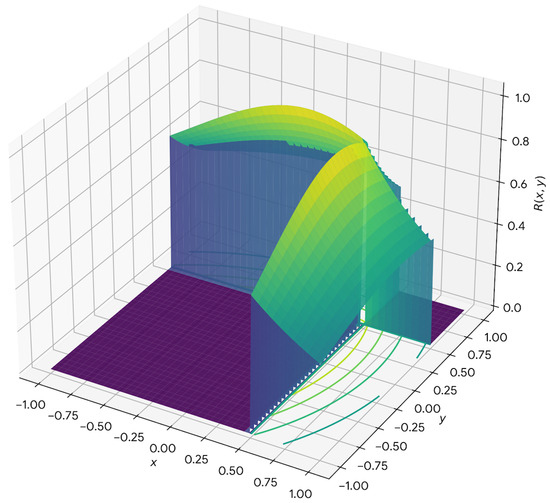
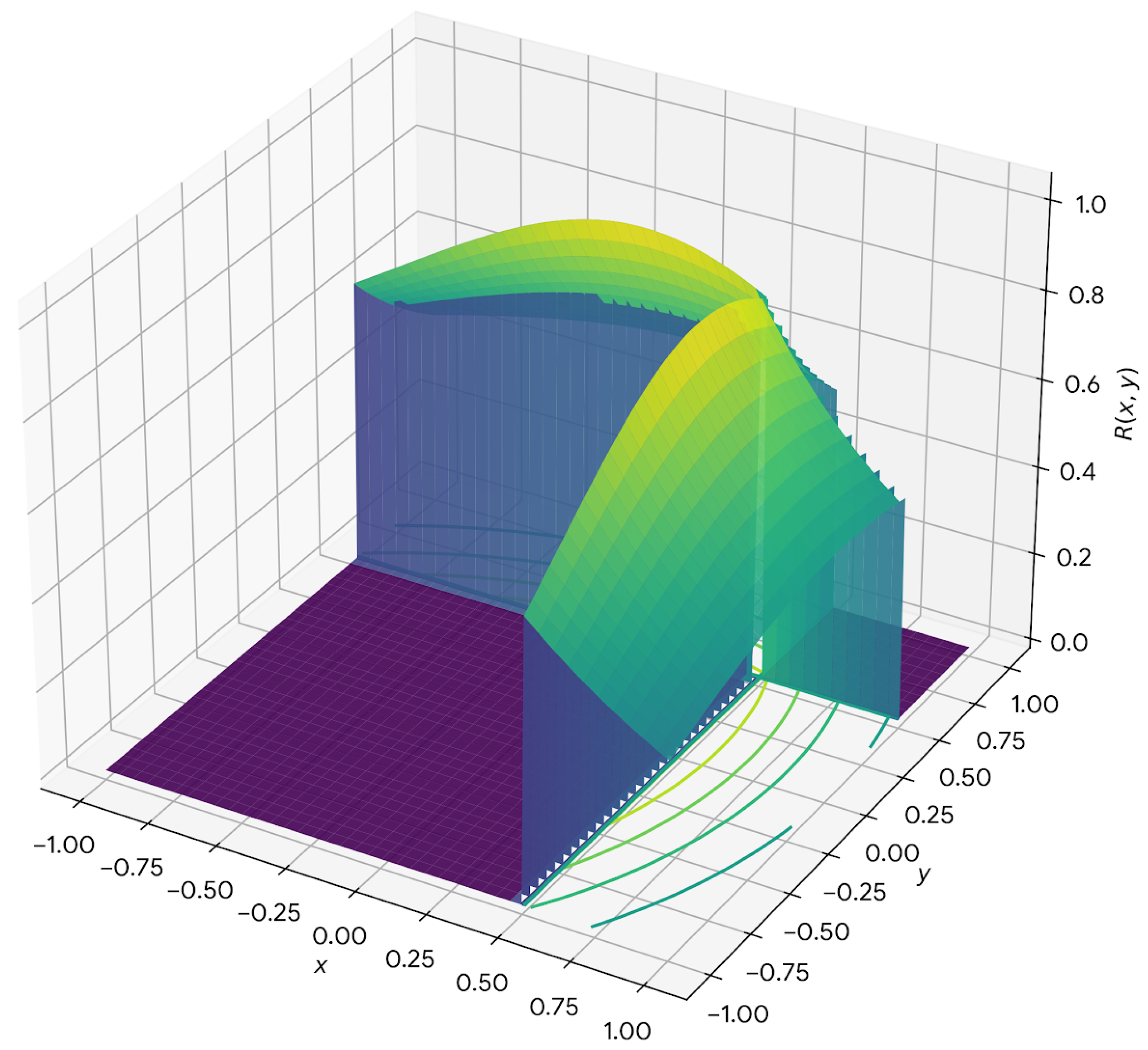
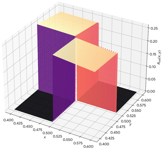
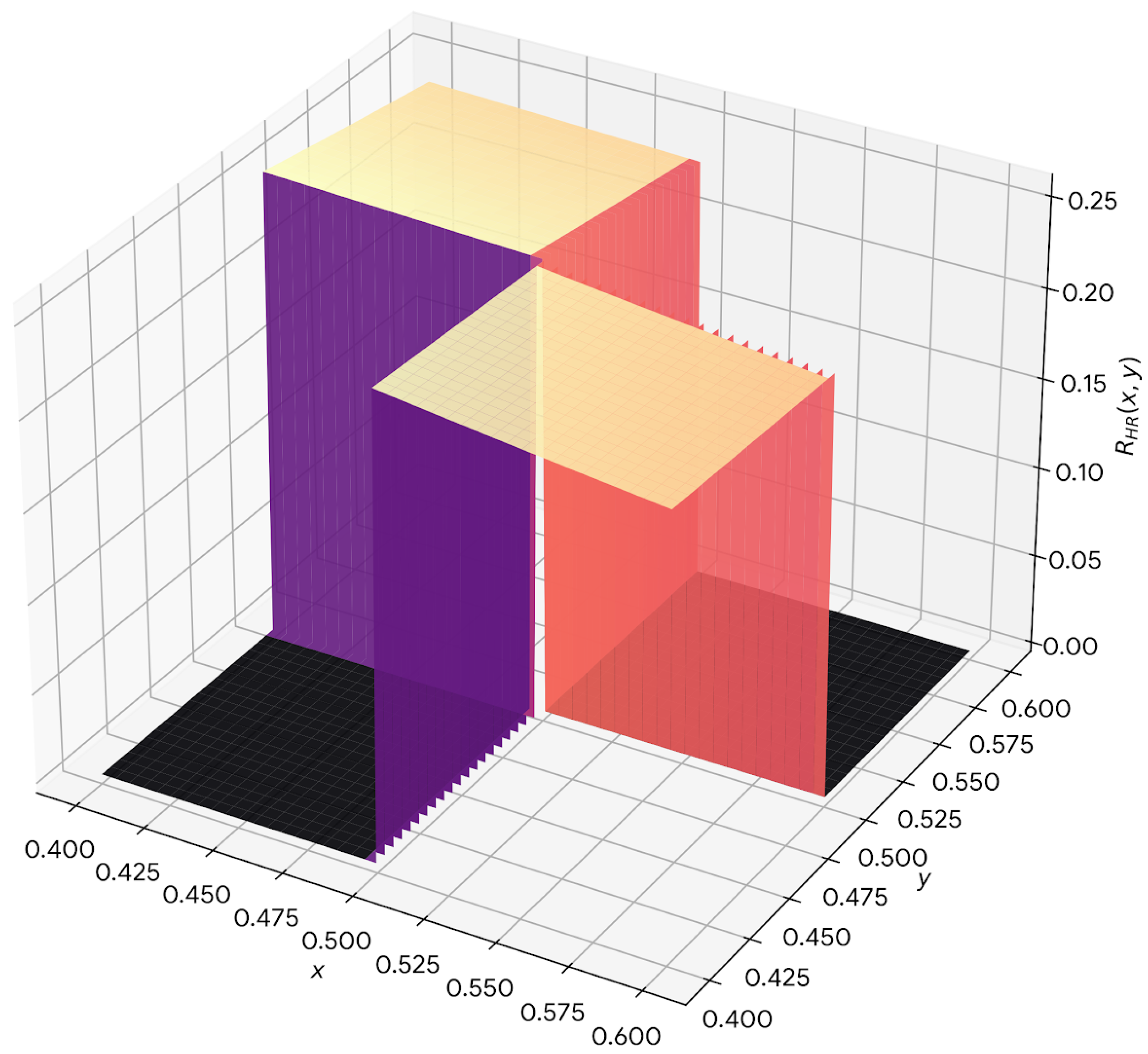
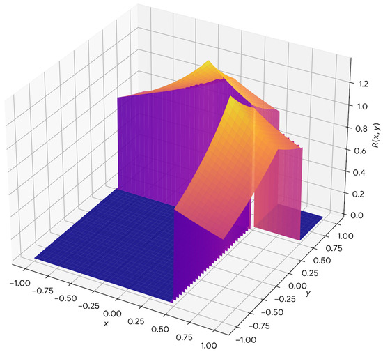
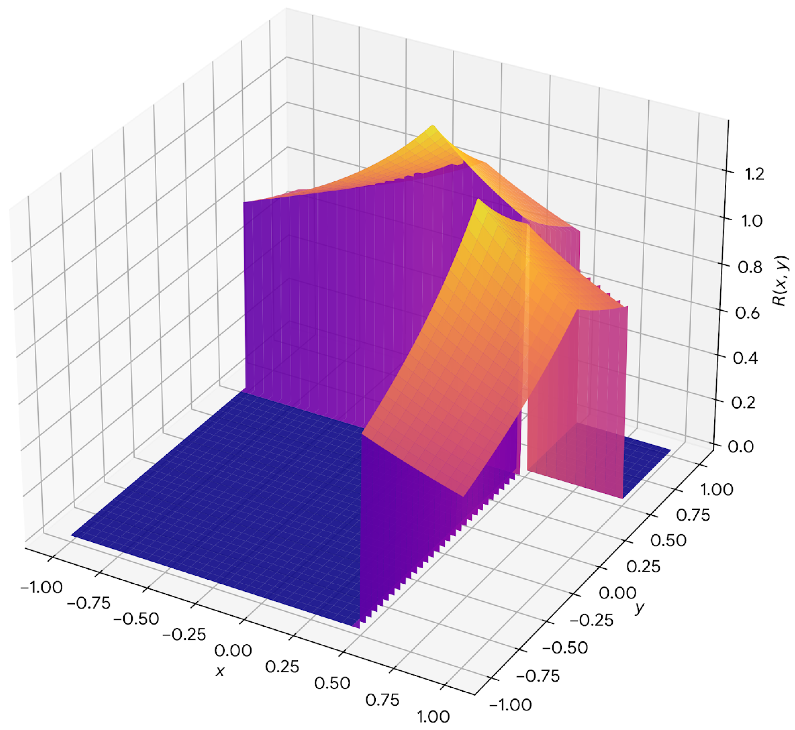
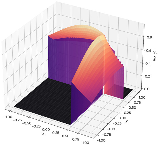
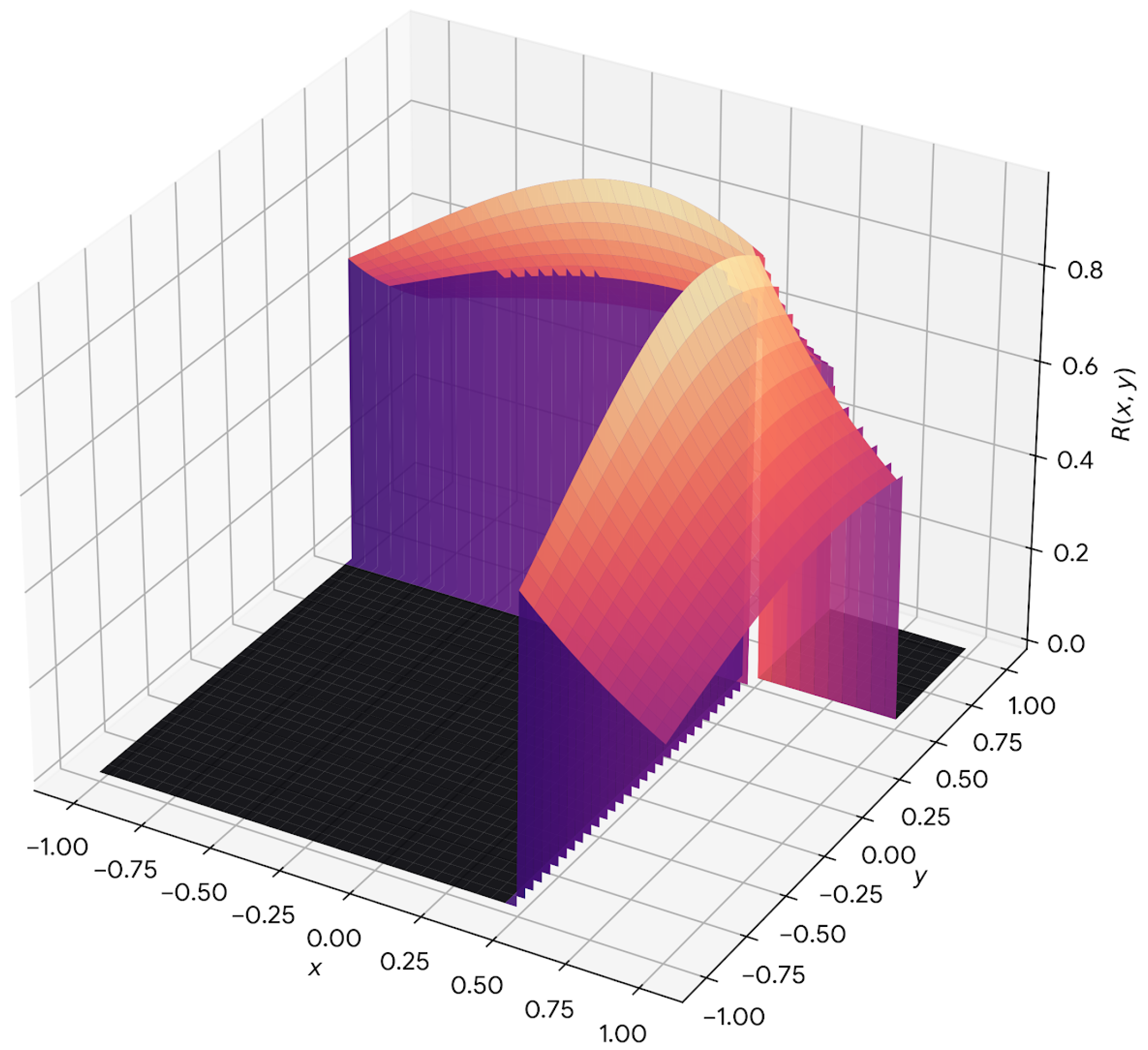
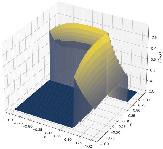
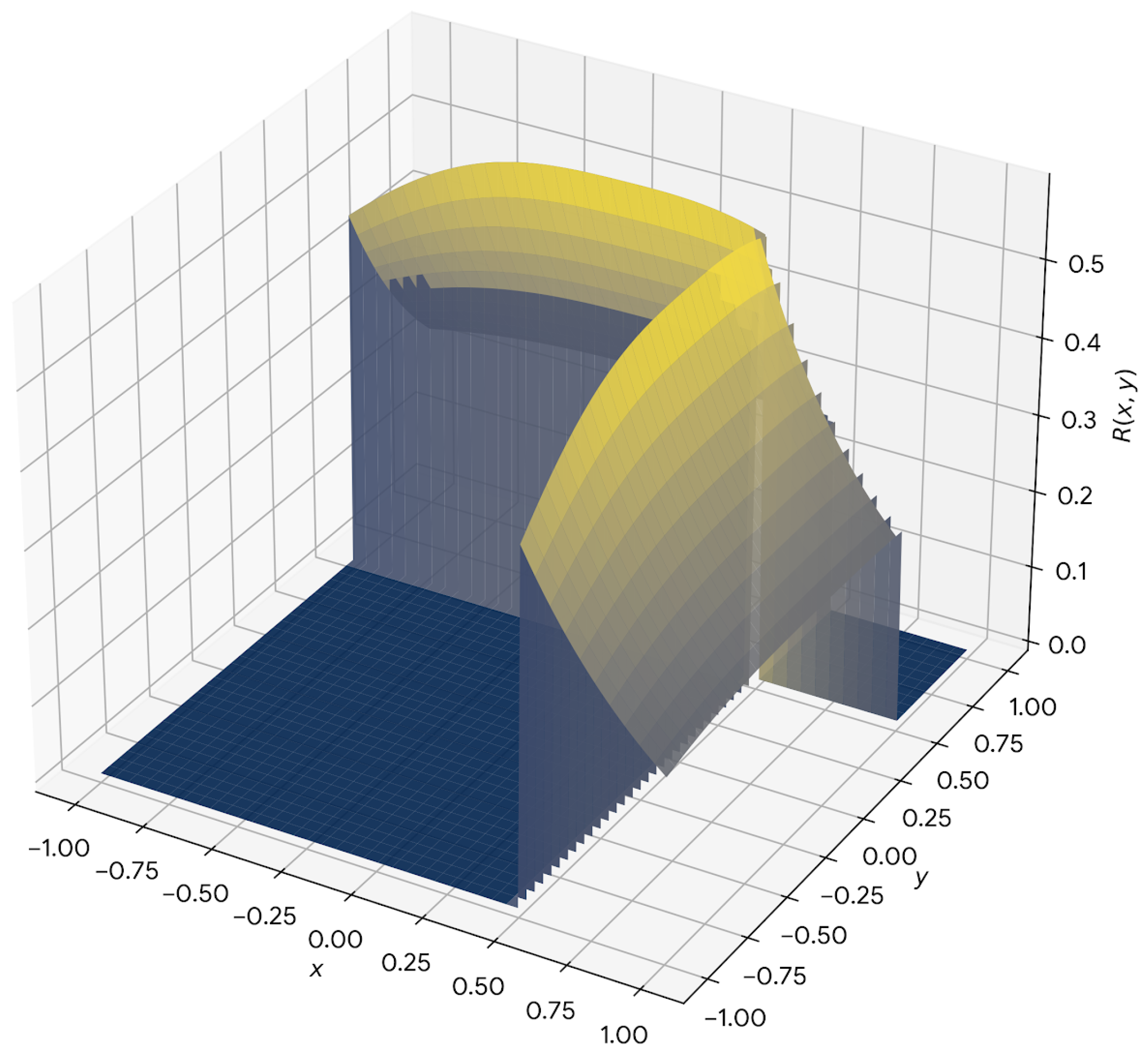
Now, we give some figures to compare the results. From Figure 1, Figure 2, Figure 3, Figure 4 and Figure 5 the following equation

$$R(x,y)={\displaystyle \frac{d^p(Tx,Ty)}{a{d}^p(x,Tx)+a{d}^p(y,Ty)+(1-2a){\displaystyle \frac{d^p(x,y)}{1+d^p(x,y)}}}}$$

is used.

Figure 1. Three-dimensional profile of the quasicontractive ratio $R(x,y)$ in Example 3 for the choice $p=2$ and $a=0.46\in (4/9,1/2)$. The surface stays strictly below 1, illustrating the rational $(a,p)-$quasicontractive behaviour of T on $[-1,1]$.

Figure 2. Hardy-Rogers violation ratio $R(x,y)$. The ratio peaks visibly above $\mathbf{1}$ in the cross-side region near the discontinuity ($x,y\approx 0.5$). This demonstrates that T fails to meet the Hardy-Rogers contraction condition, illustrating the stronger nature of this classical contraction type compared to the rational quasi-contraction.

Figure 3. Quasicontractive ratio $R(x,y)$ for parameters $p=1$ and $a=0.46$. The reduction of the metric exponent p leads to a more linear distance measure, resulting in a sharper profile along the discontinuity lines $x=0.5$ and $y=0.5$.

Figure 4. Quasicontractive ratio $R(x,y)$ for $p=2$ and $a=0.445$. As a is very close to the lower bound $4/9\approx 0.444$, the maximum of $R(x,y)$ is shown to be extremely close to 1, highlighting the boundary case for the quasicontractive condition.

Figure 5. Quasicontractive ratio $R(x,y)$ for $p=3$ and $a=0.49$. The higher exponent p and a being close to the upper bound $0.5$ result in a flatter surface, indicating a “safer” quasicontractive margin, maximum $R(x,y)$ is further below 1.

In the following, Figure 3, Figure 4 and Figure 5 illustrate the resulting conditions obtained by varying the parameters a and p.

Example 4.

With X and T as in Example (3), fix $p\in \mathbb{N}$ and $a\in \left({\left(\frac{2}{3}\right)}^p,\frac{1}{2}\right)$. For $x\le \frac{1}{2}<y$ we have $d(Tx,Ty)=1$ and $d(y,Ty)=y+1\ge \frac{3}{2}$ while $d(x,Tx)=\left|x\right|\le \frac{1}{2}$. Considering these facts in the inequality Equation (4), we obtain

$$a{d}^p(x,Tx)+a{d}^p(y,Ty)+(1-2a){\displaystyle \frac{d^p(x,y)}{1+d^p(x,y)}}\ge a{\left(\frac{3}{2}\right)}^p.$$

Since $a>{\left(\frac{2}{3}\right)}^p$, it follows that

$$d^p(Tx,Ty)=1<a{\left(\frac{3}{2}\right)}^p\le a{d}^p(x,Tx)+a{d}^p(y,Ty)+(1-2a){\displaystyle \frac{d^p(x,y)}{1+d^p(x,y)}}.$$

Hence, the inequality Equation (4) holds strictly. The Hardy-Rogers condition failure is unchanged from Example 3.

Example 3 illustrates the quadratic case $p=2$, where the rational inequality is strictly satisfied while the Hardy-Rogers condition fails. Example 4 extends this construction to arbitrary $p\in \mathbb{N}$, with admissibility interval $a\in \left({\left(\frac{2}{3}\right)}^p,\frac{1}{2}\right)$. Hence, the rational framework is not confined to quadratic growth, but applies uniformly to all exponents p, reinforcing its generality beyond the special case $p=2$.

Corollary 2.

In the compact metric space $[-1,1]$, the mapping T defined in Examples 3 and 4 is a rational $a-$quadratic quasicontraction and rational $(a,p)-$quasicontraction for suitable choices of a and p, but is not a Hardy-Rogers contraction. In particular:

(i) 

For rational $a-$quadratic quasicontraction inequality (Example 3), the admissible range is $a\in (\frac{4}{9},\frac{1}{2})$ with $p=2$.

(ii) 

For rational $(a,p)-$quasicontraction inequality (Example 4), the admissible range is $a\in ({\left(\frac{2}{3}\right)}^p,\frac{1}{2})$ for arbitrary $p\in \mathbb{N}$.

In all these cases, $0\in [-1,1]$ is the fixed point, and the Picard iteration satisfies $T^{n}x\to 0$ for every $x\in [-1,1]$.

Remark 8.

Corollary 2 and the preceding examples demonstrate that the rational $(a,p)-$quasicon- traction framework strictly extends beyond the Hardy-Rogers setting. In particular, mappings exist on compact metric spaces that fail every Hardy-Rogers inequality yet are fully admissible under our rational conditions. Consequently, the fixed-point results obtained apply more broadly, covering cases inaccessible to the Hardy-Rogers theory.

4. A Rational (a, p)−Quasicontractive Treatment of a Delayed Caputo Multi-Point Boundary Value Problem

In this section, we revisit the delayed multi-point boundary value problem studied in [19] and consider its Caputo fractional counterpart. We show that the associated Hammerstein operator fits naturally into the rational $(a,p)-$framework introduced in Section 3. In particular, we obtain a unique positive solution together with global Picard convergence by verifying that the corresponding operator is a strict rational $(a,p)-$quasicontraction on an invariant cone–ball of a Banach space.

Throughout this section, we fix $p\in \mathbb{N}$ and an order $1<\alpha \le 2.$ For a sufficiently smooth function $u:[0,1]\to \mathbb{R}$, we denote by ${}^{C}D_{0^{+}}^{\alpha }u\left(t\right)$ the Caputo derivative of order $\alpha$ with starting point 0, defined by

$$\left({}^{C}D_{0^{+}}^{\alpha }u\right)\left(t\right):={\displaystyle \frac{1}{\Gamma (2-\alpha )}}{\int }_0^t{(t-s)}^{1-\alpha }{u}^{″}\left(s\right)ds,t\in (0,1),$$

where $\Gamma$ is the Gamma function. We also use the shorthand for $t\ge 0$

$${\phi }_p\left(t\right):={\displaystyle \frac{t^p}{1+t^p}}.$$

(20)

4.1. The Delayed Fractional Multi-Point Problem and Its Green Function

We consider the delayed nonlocal Caputo boundary value problem as

$$\left\{\begin{array}{cc}{}^{C}D_{0^{+}}^{\alpha }\nu \left(t\right)+q\left(t\right)f\left(t,{\nu }_t\right)=0,\hfill & 0<t<1,\hfill \\ \nu \left(t\right)=\phi \left(t\right),\hfill & -\tau \le t\le 0,\hfill \\ {\nu }^{\prime }\left(0\right)=0,\nu \left(1\right)=\xi \nu \left(\gamma \right)+\upsilon {\nu }^{\prime }\left(\gamma \right),\hfill \end{array}\right.$$

(21)

where

$$0\le \gamma \le 1,0\le \xi <1,0\le \upsilon \le \xi (1-\gamma ),0\le \tau <\frac{1}{2}.$$

For each $t\in [0,1]$ we denote the history segment by

$${\nu }_t\left(\theta \right):=\nu (t+\theta ),\theta \in [-\tau ,0].$$

We assume that

$$\begin{array}{cc}\hfill & \phi \in C\left(\right[-\tau ,0],[0,\infty \left)\right),\phi \left(0\right)=0,\hfill \\ \hfill & f\in C\left([0,1]\times C\left(\right[-\tau ,0],[0,\infty \left)\right),[0,\infty )\right),\hfill \\ \hfill & q\in L^1\left([0,1]\right),q\left(t\right)\ge 0\mathrm{a}.\mathrm{e}.\mathrm{on}[0,1],\hfill \\ \hfill & \mathrm{and}q\not\equiv 0\mathrm{on}\mathrm{any}\mathrm{subinterval}\mathrm{of}[0,1].\hfill \end{array}$$

(22)

Initially, we investigate the associated linear fractional problem

$$\left\{\begin{array}{cc}{}^{C}D_{0^{+}}^{\alpha }u\left(t\right)+\kappa \left(t\right)=0,\hfill & 0<t<1,\hfill \\ u^{\prime }\left(0\right)=0,u\left(1\right)=\xi u\left(\gamma \right)+\upsilon u^{\prime }\left(\gamma \right),\hfill \end{array}\right.$$

(23)

for a given $\kappa \in C\left(\right[0,1],\mathbb{R})$.

For $\beta >0$, we recall the Riemann-Liouville fractional integral as

$$\left(I^{\beta }\kappa \right)\left(t\right):={\displaystyle \frac{1}{\Gamma \left(\beta \right)}}{\int }_0^t{(t-s)}^{\beta -1}\kappa \left(s\right)ds,t\in [0,1].$$

It is well known that any solution of Equation (23) can be represented in terms of $I^{\alpha }\kappa$ and its first derivative.

We begin by explaining the Green function for the fractional multi-point problem.

Lemma 2.

Let $\kappa \in C\left(\right[0,1],\mathbb{R})$ and the parameters $\gamma ,\xi ,\upsilon$ satisfy the following conditions

$$0\le \gamma \le 1,0\le \xi <1,0\le \upsilon \le \xi (1-\gamma ),$$

and $1<\alpha \le 2$. Then the boundary value problem in Equation (23) admits a unique solution $u\in C^1\left([0,1]\right)$ such that ${}^{C}D_{0^{+}}^{\alpha }u\in C\left((0,1)\right)$, and

$$u\left(t\right)={\int }_0^1{G}_{\alpha }(t,\rho )\kappa \left(\rho \right)d\rho ,0\le t\le 1,$$

(24)

where $G_{\alpha }:{[0,1]}^2\to \mathbb{R}$ is a Green function. Moreover,

(i) 

$G_{\alpha }$ is continuous on ${[0,1]}^2$ and, for each fixed $\rho \in [0,1]$, the function $t\mapsto G_{\alpha }(t,\rho )$ is piecewise $C^1$ on $[0,1]$ and satisfies

$${\left({}^{C}D_{0^{+}}^{\alpha }\alpha \right)}_t{G}_{\alpha }(t,\rho )=0\mathrm{for}t\ne \rho ;$$

(ii) 

$G_{\alpha }(t,\rho )\ge 0$ for all $(t,\rho )\in {[0,1]}^2$;

(iii) 

there exist constants $\omega \in (0,1)$ and $C_G>0$, depending only on $\gamma ,\xi ,\upsilon ,\alpha$, such that

$$(1-\omega )(1-{\rho }^{\alpha -1})\le G_{\alpha }(t,\rho )\le C_G(1-{\rho }^{\alpha -1}),t\in [0,\omega ],\rho \in [0,1].$$

(25)

Proof. 

We briefly recall the standard construction for Caputo problems. Since the homogeneous equation

$${}^{C}D_{0^{+}}^{\alpha }u\left(t\right)=0$$

has linearly independent solutions 1 and t for $1<\alpha \le 2$, any solution of Equation (23) can be written as

$$u\left(t\right)=c_1+c_{2}t-\left(I^{\alpha }\kappa \right)\left(t\right),0\le t\le 1,$$

where $I^{\alpha }\kappa$ is the Riemann-Liouville fractional integral of order $\alpha$. Differentiating and using the property ${\displaystyle \frac{d}{dt}}{I}^{\alpha }\kappa =I^{\alpha -1}\kappa$, we obtain

$$u^{\prime }\left(t\right)=c_2-\left(I^{\alpha -1}\kappa \right)\left(t\right).$$

The first boundary condition $u^{\prime }\left(0\right)=0$ yields $c_2=0$, hence

$$u\left(t\right)=c_1-\left(I^{\alpha }\kappa \right)\left(t\right),u^{\prime }\left(t\right)=-\left(I^{\alpha -1}\kappa \right)\left(t\right).$$

(26)

We now impose the multi-point boundary condition at $t=1$. From Equation (26) we get

$$u\left(1\right)=c_1-\left(I^{\alpha }\kappa \right)\left(1\right)=c_1-{\displaystyle \frac{1}{\Gamma \left(\alpha \right)}}{\int }_0^1{(1-\rho )}^{\alpha -1}\kappa \left(\rho \right)d\rho ,$$

$$u\left(\gamma \right)=c_1-\left(I^{\alpha }\kappa \right)\left(\gamma \right)=c_1-{\displaystyle \frac{1}{\Gamma \left(\alpha \right)}}{\int }_0^{\gamma }{(\gamma -\rho )}^{\alpha -1}\kappa \left(\rho \right)d\rho ,$$

and

$$u^{\prime }\left(\gamma \right)=-\left(I^{\alpha -1}\kappa \right)\left(\gamma \right)=-{\displaystyle \frac{1}{\Gamma (\alpha -1)}}{\int }_0^{\gamma }{(\gamma -\sigma )}^{\alpha -2}\kappa \left(\sigma \right)d\sigma .$$

Therefore, the condition $u\left(1\right)=\xi u\left(\gamma \right)+\upsilon u^{\prime }\left(\gamma \right)$ becomes

$$\begin{array}{cc}\hfill c_1-{\displaystyle \frac{1}{\Gamma \left(\alpha \right)}}{\int }_0^1{(1-\rho )}^{\alpha -1}\kappa \left(\rho \right)d\rho =& \xi \left[c_1-{\displaystyle \frac{1}{\Gamma \left(\alpha \right)}}{\int }_0^{\gamma }{(\gamma -\rho )}^{\alpha -1}\kappa \left(\rho \right)d\rho \right]\hfill \\ \hfill & +\upsilon \left[-{\displaystyle \frac{1}{\Gamma (\alpha -1)}}{\int }_0^{\gamma }{(\gamma -\sigma )}^{\alpha -2}\kappa \left(\sigma \right)d\sigma \right].\hfill \end{array}$$

Collecting the terms containing $c_1$ on the left-hand side, we obtain

$$(1-\xi )c_1={\displaystyle \frac{1}{\Gamma \left(\alpha \right)}}{\int }_0^1{(1-\rho )}^{\alpha -1}\kappa \left(\rho \right)d\rho -{\displaystyle \frac{\xi }{\Gamma \left(\alpha \right)}}{\int }_0^{\gamma }{(\gamma -\rho )}^{\alpha -1}\kappa \left(\rho \right)d\rho +{\displaystyle \frac{\upsilon }{\Gamma (\alpha -1)}}{\int }_0^{\gamma }{(\gamma -\sigma )}^{\alpha -2}\kappa \left(\sigma \right)d\sigma .$$

Since $0\le \xi <1$, division by $(1-\xi )$ yields

$$c_1={\displaystyle \frac{1}{1-\xi }}\left[{\displaystyle \frac{1}{\Gamma \left(\alpha \right)}}{\int }_0^1{(1-\rho )}^{\alpha -1}\kappa \left(\rho \right)d\rho -{\displaystyle \frac{\xi }{\Gamma \left(\alpha \right)}}{\int }_0^{\gamma }{(\gamma -\rho )}^{\alpha -1}\kappa \left(\rho \right)d\rho +{\displaystyle \frac{\upsilon }{\Gamma (\alpha -1)}}{\int }_0^{\gamma }{(\gamma -\sigma )}^{\alpha -2}\kappa \left(\sigma \right)d\sigma \right].$$

(27)

Substituting Equation (27) into Equation (26), we obtain $u\left(t\right)$ as a linear combination of fractional integrals of $\kappa$ with kernels depending on t and $\rho$. Splitting all integrals over $[0,1]$ into the subintervals $[0,t]$ and $[t,1]$ and rearranging the resulting expressions, we can rewrite $u\left(t\right)$ in the form

$$u\left(t\right)={\int }_0^1{G}_{\alpha }(t,\rho )\kappa \left(\rho \right)d\rho ,$$

where $G_{\alpha }(t,\rho )$ is given by an explicit piecewise formula involving the kernels ${(t-\rho )}^{\alpha -1}$, ${(1-\rho )}^{\alpha -1}$ and their shifted versions. A straightforward computation shows that $G_{\alpha }$ can be chosen as a continuous function on ${[0,1]}^2$, piecewise $C^1$ in the $t-$variable, and such that ${\left({}^{C}D_{0^{+}}^{\alpha }\right)}_t{G}_{\alpha }(t,\rho )=0$ whenever $t\ne \rho$. This yields the representation Equation (24) and the regularity statement (i).

The positivity in (ii) follows from a comparison argument analogous to the classical second-order case: for each fixed $\rho \in [0,1]$, the function $g_{\rho }\left(t\right):=G_{\alpha }(t,\rho )$ solves a linear fractional equation with a negative jump singularity at $t=\rho$ and the given mixed boundary conditions. Using the maximum principle for Caputo fractional equations, one checks that $g_{\rho }$ is a non-negative combination of non-negative kernels, hence $G_{\alpha }(t,\rho )\ge 0$.

Finally, to obtain the bounds in (iii), we exploit the explicit formula for $G_{\alpha }(t,\rho )$ and the fact that the building blocks are fractional integrals of continuous functions. One shows that there exists a constant $C_G>0$ such that

$$0\le G_{\alpha }(t,\rho )\le C_G(1-{\rho }^{\alpha -1}),(t,\rho )\in {[0,1]}^2,$$

and that on a smaller time interval $[0,\omega ]$, with $\omega \in (0,1)$ depending only on $\gamma ,\xi ,\upsilon ,\alpha$, the function $G_{\alpha }(t,\rho )$ is bounded below by a positive multiple of $(1-{\rho }^{\alpha -1})$, namely

$$G_{\alpha }(t,\rho )\ge (1-\omega )(1-{\rho }^{\alpha -1}),t\in [0,\omega ],\rho \in [0,1].$$

This yields Equation (25) and completes the proof. □

Using Lemma 2, problem Equation (21) can be rewritten as an integral equation. For $t\in [0,1]$, a classical solution $\nu$ of Equation (21) satisfies

$$\nu \left(t\right)={\int }_0^1{G}_{\alpha }(t,\rho )q\left(\rho \right)f\left(\rho ,{\nu }_{\rho }\right)d\rho ,0\le t\le 1,$$

(28)

while the values on $[-\tau ,0]$ are prescribed by $\nu \left(t\right)=\phi \left(t\right)$. Conversely, any $\nu$ satisfying Equation (28) with the given history and with $G_{\alpha }$ as in Lemma 2 solves Equation (21). This is the starting point of the Hammerstein formulation.

4.2. Hammerstein Formulation on a Cone-Ball

Let

$$X:=C\left(\right[-\tau ,1],\mathbb{R}),$$

and

$$\parallel x\parallel :=\underset{t\in [-\tau ,1]}{sup}\left|x\left(t\right)\right|.$$

We equip the set X with the metric $d(x,y):=\parallel x-y\parallel$, so that $(X,d)$ is a Banach space. For each $t\in [0,1]$ and $x\in X$ we write, for all $\theta \in [-\tau ,0]$,

$$x_t\left(\theta \right):=x(t+\theta ),$$

so that $x_t\in C([-\tau ,0],\mathbb{R})$ and $\parallel x_t{\parallel }_{C[-\tau ,0]}\le \parallel x\parallel$.

We consider the cone

$$P:=\left\{x\in X:x\left(t\right)\ge 0\mathrm{for}t\in [0,1],x\left(t\right)=0\mathrm{for}t\in [-\tau ,0]\right\},$$

which encodes the positivity and history structure of Equation (21).

The nonlinearity f appearing in Equation (21) is assumed to satisfy the following growth and Lipschitz conditions.

(H1)

Linear growth: There exists $M\ge 0$ such that

$$0\le f(t,\psi )\le M\left(1+{\parallel \psi \parallel }_{C[-\tau ,0]}\right)\mathrm{for}\mathrm{all}t\in [0,1],\psi \in C([-\tau ,0],[0,\infty )).$$

(H2)

Lipschitz continuity: There exists $L>0$ such that

$$|f(t,\psi )-f(t,\chi )|\le {L\parallel \psi -\chi \parallel }_{C[-\tau ,0]}\mathrm{for}\mathrm{all}t\in [0,1],\psi ,\chi \in C([-\tau ,0],[0,\infty )).$$

Using the fractional Green representation Equation (28), we define the Hammerstein operator $T:X\to X$ by

$$\left(Tx\right)\left(t\right):=\left\{\begin{array}{cc}{\displaystyle {\int }_0^1{G}_{\alpha }(t,\rho )q\left(\rho \right)f\left(\rho ,x_{\rho }+{\phi }_{\rho }\right)d\rho ,}\hfill & 0\le t\le 1,\hfill \\ 0,\hfill & -\tau \le t\le 0,\hfill \end{array}\right.$$

(29)

where ${\phi }_{\rho }\left(\theta \right):=\phi (\rho +\theta )$, $\theta \in [-\tau ,0]$. By Equation (22) and Lemma 2, the integrand in Equation (29) is continuous in $(t,\rho )$; hence $Tx\in X$ for every $x\in X$.

Moreover, from $G_{\alpha }(t,\rho )\ge 0$, $q\left(\rho \right)\ge 0$ and $f(\rho ,·)\ge 0$, we obtain $\left(Tx\right)\left(t\right)\ge 0$ for $t\in [0,1]$, while by definition $\left(Tx\right)\left(t\right)=0$ on $[-\tau ,0]$. Therefore $T\left(P\right)\subset P$.

A fixed point $x\in P$ of T yields a function

$${\nu }_x\left(t\right):=\left\{\begin{array}{cc}\phi \left(t\right),\hfill & -\tau \le t\le 0,\hfill \\ x\left(t\right),\hfill & 0\le t\le 1,\hfill \end{array}\right.$$

which satisfies Equation (28) and hence problem Equation (21). Conversely, any solution $\nu$ of Equation (21) defines $x\left(t\right):=\nu \left(t\right)$ for $t\in [0,1]$ and $x\left(t\right):=0$ for $t\in [-\tau ,0]$, and this x is a fixed point of T.

We now restrict T to an invariant cone–ball. Using the upper bound in Equation (25), we set

$$B:=C_G{\int }_0^1(1-{\rho }^{\alpha -1})q\left(\rho \right)d\rho ,$$

(30)

where $C_G$ is as in Lemma 2. Then, Lemma 2 gives

$$0\le G_{\alpha }(t,\rho )\le C_G(1-{\rho }^{\alpha -1}),(t,\rho )\in {[0,1]}^2.$$

In the following lemma, we obtain the criteria for the invariance of the cone–ball and the compactness.

Lemma 3.

Assume that the properties claimed in Equation (22) and (H1) hold. Let B be given by Equation (30) and set

$$C_R:=P\cap \{x\in X:\parallel x\parallel \le R\},R>0.$$

If R satisfies the inequality

$$MB\left(1+{\parallel \phi \parallel }_{C[-\tau ,0]}+R\right)\le R,$$

(31)

then

(i) 

$T\left(C_R\right)\subset C_R$;

(ii) 

$T\left(C_R\right)$ is relatively compact in X.

Proof. 

We divide this proof into two steps.

• Step 1: We demonstrate the invariance of $C_R$. Let $x\in C_R$ be arbitrary and fix $t\in [0,1]$. From Equation (29), the bound $G_{\alpha }(t,\rho )\le C_G(1-{\rho }^{\alpha -1})$ and the growth condition (H1) we obtain

$$\begin{array}{cc}\hfill \left|\right(Tx\left)\right(t\left)\right|& \le {\int }_0^1{G}_{\alpha }(t,\rho )q\left(\rho \right)f\left(\rho ,x_{\rho }+{\phi }_{\rho }\right)d\rho \hfill \\ \hfill & \le {\int }_0^1{C}_G(1-{\rho }^{\alpha -1})q\left(\rho \right)M\left(1+\parallel x_{\rho }+{\phi }_{\rho }{\parallel }_{C[-\tau ,0]}\right)d\rho .\hfill \end{array}$$

For each $\rho \in [0,1]$ and $\theta \in [-\tau ,0]$ we have

$$|x_{\rho }\left(\theta \right)|=|x(\rho +\theta )|\le \parallel x\parallel \le R,$$

and

$$|{\phi }_{\rho }{\left(\theta \right)|=|\phi (\rho +\theta )|\le \parallel \phi \parallel }_{C[-\tau ,0]}.$$

Hence

$$\parallel x_{\rho }+{\phi }_{\rho }{\parallel }_{C[-\tau ,0]}\le \parallel x\parallel +{\parallel \phi \parallel }_{C[-\tau ,0]}\le R+{\parallel \phi \parallel }_{C[-\tau ,0]}.$$

Substituting this estimate into the previous inequality yields

$$\begin{array}{cc}\hfill \left|\right(Tx\left)\right(t\left)\right|& \le M{C}_G{\int }_0^1(1-{\rho }^{\alpha -1})q\left(\rho \right)\left(1+R+{\parallel \phi \parallel }_{C[-\tau ,0]}\right)d\rho \hfill \\ \hfill & =M{C}_G\left(1+R+{\parallel \phi \parallel }_{C[-\tau ,0]}\right){\int }_0^1(1-{\rho }^{\alpha -1})q\left(\rho \right)d\rho \hfill \\ \hfill & =MB\left(1+R+{\parallel \phi \parallel }_{C[-\tau ,0]}\right),\hfill \end{array}$$

where B is defined in Equation (30). Taking the supremum over $t\in [0,1]$ and observing that $\left(Tx\right)\left(t\right)=0$ on $[-\tau ,0]$, we obtain

$$\parallel Tx\parallel \le MB\left(1+R+{\parallel \phi \parallel }_{C[-\tau ,0]}\right).$$

(32)

If R satisfies Equation (31), then the right-hand side of Equation (32) is bounded by R, which means

$$\parallel Tx\parallel \le R.$$

Since we know $T\left(P\right)\subset P$, this implies $T\left(C_R\right)\subset C_R$ and proves (i).

Step 2: In this step, we prove the relative compactness of the set $T\left(C_R\right)$. First, Equation (32) shows that $\parallel Tx\parallel \le R$ for every $x\in C_R$, so the set $T\left(C_R\right)$ is uniformly bounded in X.

Next, we investigate the equicontinuity of the family $\{Tx:x\in C_R\}$ on $[0,1]$. Let $x\in C_R$ and $t,s\in [0,1]$. Then

$$|(Tx)(t)-(Tx)(s)|\le {\int }_0^1|G_{\alpha }(t,\rho )-G_{\alpha }(s,\rho )|q\left(\rho \right)f\left(\rho ,x_{\rho }+{\phi }_{\rho }\right)d\rho .$$

Using the growth condition (H1) and the estimate for $\parallel x_{\rho }+{\phi }_{\rho }{\parallel }_{C[-\tau ,0]}$ derived above, we obtain

$$|\left(Tx\right)\left(t\right)-\left(Tx\right)\left(s\right)|\le M\left(1+R+{\parallel \phi \parallel }_{C[-\tau ,0]}\right){\int }_0^1|G_{\alpha }(t,\rho )-G_{\alpha }(s,\rho )|q\left(\rho \right)d\rho .$$

The integrand is dominated by

$$|G_{\alpha }(t,\rho )-G_{\alpha }(s,\rho )|q\left(\rho \right)\le 2C_G(1-{\rho }^{\alpha -1})q\left(\rho \right),$$

which is integrable on $[0,1]$ by Equation (22). Since $G_{\alpha }(·,\rho )$ is continuous uniformly in $\rho$ on the compact set ${[0,1]}^2$, it follows that

$${\int }_0^1|G_{\alpha }(t,\rho )-G_{\alpha }(s,\rho )|q\left(\rho \right)d\rho \to 0,$$

as $t\to s$. The convergence is independent of $x\in C_R$ because the prefactor $M(1+R+\parallel \phi {\parallel }_{C[-\tau ,0]})$ does not depend on x. Thus, the family $\{Tx:x\in C_R\}$ is equicontinuous on $[0,1]$. On $[-\tau ,0]$, all functions $Tx$ vanish identically; hence, equicontinuity follows automatically in this setting.

We have shown that $T\left(C_R\right)$ is uniformly bounded and equicontinuous on the compact interval $[-\tau ,1]$. By the Arzelà-Ascoli theorem, $T\left(C_R\right)$ is relatively compact in $X=C\left(\right[-\tau ,1],\mathbb{R})$, which proves (ii). □

Remark 9.

The condition Equation (31) is satisfiable whenever $MB<1$, because the inequality

$$MB\left(1+{\parallel \phi \parallel }_{C[-\tau ,0]}+R\right)\le R$$

can be rewritten as

$$R(1-MB)\ge MB\left(1+{\parallel \phi \parallel }_{C[-\tau ,0]}\right),$$

so any

$$R\ge {\displaystyle \frac{MB\left(1+{\parallel \phi \parallel }_{C[-\tau ,0]}\right)}{1-MB}}$$

is admissible. In particular, the smallness of the product $MB$ encodes the balance between the growth of f and the size of the fractional Green kernel.

4.3. Rational $(a,p)-$Quasicontractivity of the Hammerstein Operator

We now exploit the Lipschitz condition (H2) to show that T satisfies a rational $(a,p)-$quasicontractive inequality on the cone-ball $C_R$.

Lemma 4.

Assume that the properties given in Equation (22) and (H2) hold. Let B be as in Equation (30) and set

$$K:=LB.$$

Then for all $x,y\in X$ we have

$$\parallel Tx-Ty\parallel \le K\parallel x-y\parallel .$$

(33)

In particular, for every $p\in \mathbb{N}$ and $x,y\in C_R$,

$$d{(Tx,Ty)}^p\le {\Theta }_p{\phi }_p\left(d(x,y)\right),{\Theta }_p:=K^p\left(1+{\left(2R\right)}^p\right),$$

(34)

where $d(x,y):=\parallel x-y\parallel$ and ${\phi }_p$ is defined in Equation (20).

Proof. 

Let $x,y\in X$ and $t\in [0,1]$ be arbitrary. Using Equation (29) we write

$$(Tx)(t)-(Ty)(t)={\int }_0^1{G}_{\alpha }(t,\rho )q\left(\rho \right)\left[f\left(\rho ,x_{\rho }+{\phi }_{\rho }\right)-f\left(\rho ,y_{\rho }+{\phi }_{\rho }\right)\right]d\rho .$$

Taking absolute values and applying the Lipschitz property (H2), we obtain

$$\begin{array}{cc}\hfill \left|\right(Tx\left)\right(t)-(Ty\left)\right(t\left)\right|& \le {\int }_0^1{G}_{\alpha }(t,\rho )q\left(\rho \right)\left|f\left(\rho ,x_{\rho }+{\phi }_{\rho }\right)-f\left(\rho ,y_{\rho }+{\phi }_{\rho }\right)\right|d\rho \hfill \\ \hfill & \le {\int }_0^1{G}_{\alpha }(t,\rho )q\left(\rho \right)L{\parallel x_{\rho }-y_{\rho }\parallel }_{C[-\tau ,0]}d\rho .\hfill \end{array}$$

For each $\rho \in [0,1]$ and $\theta \in [-\tau ,0]$ we have

$$|x_{\rho }\left(\theta \right)-y_{\rho }\left(\theta \right)|=|x(\rho +\theta )-y(\rho +\theta )|\le \parallel x-y\parallel ,$$

hence $\parallel x_{\rho }-y_{\rho }{\parallel }_{C[-\tau ,0]}\le \parallel x-y\parallel$. Thus

$$|(Tx)(t)-(Ty)(t)|\le L\parallel x-y\parallel {\int }_0^1{G}_{\alpha }(t,\rho )q\left(\rho \right)d\rho .$$

Using the bound $G_{\alpha }(t,\rho )\le C_G(1-{\rho }^{\alpha -1})$ and the definition of B in Equation (30), we obtain

$$\begin{array}{cc}\hfill \left|\right(Tx\left)\right(t)-(Ty\left)\right(t\left)\right|& \le L\parallel x-y\parallel {\int }_0^1{C}_G(1-{\rho }^{\alpha -1})q\left(\rho \right)d\rho \hfill \\ \hfill & =LB\parallel x-y\parallel .\hfill \end{array}$$

Taking the supremum over $t\in [0,1]$ and noting that $Tx$ and $Ty$ vanish on $[-\tau ,0]$, we obtain

$$\parallel Tx-Ty\parallel \le K\parallel x-y\parallel ,$$

with $K:=LB$, proving Equation (33).

Now suppose that $x,y\in C_R$. Then, by definition of $C_R$, we know that

$$\parallel x\parallel \le R,\parallel y\parallel \le R,$$

so that

$$d(x,y)=\parallel x-y\parallel \le \parallel x\parallel +\parallel y\parallel \le 2R.$$

Let $r:=d(x,y)$ for brevity. From Equation (33) we have

$$d(Tx,Ty)\le Kr.$$

Raising both sides to the $p-$th power gives

$$d{(Tx,Ty)}^p\le K^p{r}^p.$$

On the other hand, by the definition of ${\phi }_p$,

$${\phi }_p\left(r\right)={\displaystyle \frac{r^p}{1+r^p}},$$

so that

$$r^p= \left(1+r^p\right){\phi }_p\left(r\right).$$

Since $r\le 2R$, we have $r^p\le {\left(2R\right)}^p$, hence $1+r^p\le 1+{\left(2R\right)}^p$. Therefore

$$r^p=(1+r^p){\phi }_p\left(r\right)\le \left(1+{\left(2R\right)}^p\right){\phi }_p\left(r\right).$$

Combining this with the previous estimate shows that

$$d{(Tx,Ty)}^p\le K^p{r}^p\le K^p\left(1+{\left(2R\right)}^p\right){\phi }_p\left(r\right),$$

which is precisely Equation (34) with ${\Theta }_p:=K^p\left(1+{\left(2R\right)}^p\right)$. □

In the following, we demonstrate that the mapping T is a rational $(a,p)-$quasicontraction, which is one of the main results of this study.

Proposition 1.

Assume Equation (22), (H1)–(H2) and let $R>0$ satisfy Equation (31). Let $p\in \mathbb{N}$ and ${\Theta }_p$ be given by Equation (34) and suppose that

$${\Theta }_p<1.$$

(35)

Choose $a\in (0,\frac{1}{2})$ such that

$$0<a<{\displaystyle \frac{1-{\Theta }_p}{2}}.$$

(36)

Then the Hammerstein operator $T:C_R\to C_R$ is a strict rational $(a,p)-$quasicontraction in the sense of Definition 2; that is,

$$d^p(Tx,Ty)\le a{d}^p(x,Tx)+a{d}^p(y,Ty)+(1-2a){\phi }_p\left(d(x,y)\right)$$

(37)

for all $x,y\in C_R$, with strict inequality whenever $x\ne y$.

Proof. 

Let $x,y\in C_R$ be arbitrary and put

$$r:=d(x,y)=\parallel x-y\parallel \ge 0.$$

By Lemma 4, we know that the operator T satisfies the inequality

$$d^p(Tx,Ty)\le {\Theta }_p{\phi }_p\left(r\right),$$

(38)

where

$${\phi }_p\left(r\right):={\displaystyle \frac{r^p}{1+r^p}},r\ge 0,$$

and the constant ${\Theta }_p>0$ depends only on the data of the problem and not on $x,y$.

• Step 1: We prove the existence of an admissible parameter $a.$ By the assumption Equation (35) we have ${\Theta }_p<1$, hence $1-{\Theta }_p>0$. Therefore, the open interval

$$I:=\left(0,{\displaystyle \frac{1-{\Theta }_p}{2}}\right)$$

is nonempty. Any $a\in I$ satisfies $0<a<\frac{1}{2}$ and also

$$1-2a-{\Theta }_p=(1-{\Theta }_p)-2a>(1-{\Theta }_p)-(1-{\Theta }_p)=0.$$

(39)

In particular,

$${\Theta }_p<1-2a,$$

(40)

which will be the key inequality in what follows. Fix once and for all such an $a\in I$.

• Step 2: In this step, we compare the coefficients. Since ${\phi }_p\left(r\right)\ge 0$ for every $r\ge 0$, multiplying Equation (40) by ${\phi }_p\left(r\right)$ yields

$${\Theta }_p{\phi }_p\left(r\right)\le (1-2a){\phi }_p\left(r\right),$$

(41)

with strict inequality whenever ${\phi }_p\left(r\right)>0$, that is whenever $r>0$, equivalently $x\ne y$. Combining Equations (38) and (41) we obtain

$$d^p(Tx,Ty)\le {\Theta }_p{\phi }_p\left(r\right)\le (1-2a){\phi }_p\left(r\right),$$

(42)

and if $x\ne y$ then the last inequality is in fact strict

$$d^p(Tx,Ty)<(1-2a){\phi }_p\left(r\right).$$

(43)

• Step 3: Observe that for all $x,y\in C_R$ we have

$$d^p(x,Tx)\ge 0,d^p(y,Ty)\ge 0.$$

Hence, multiplying by $a>0$ preserves non-negativity

$$a{d}^p(x,Tx)\ge 0,a{d}^p(y,Ty)\ge 0.$$

Adding these two non-negative quantities to the right-hand side of Equation (42), we get

$$\begin{array}{cc}\hfill d^p(Tx,Ty)& \le (1-2a){\phi }_p\left(r\right)\hfill \\ \hfill & \le a{d}^p(x,Tx)+a{d}^p(y,Ty)+(1-2a){\phi }_p\left(r\right).\hfill \end{array}$$

This is exactly the inequality Equation (37).

If in addition $x\ne y$, then $r=d(x,y)>0$ and hence ${\phi }_p\left(r\right)>0$. In that case Equation (43) holds, and therefore

$$\begin{array}{cc}\hfill d^p(Tx,Ty)& <(1-2a){\phi }_p\left(r\right)\hfill \\ \hfill & \le a{d}^p(x,Tx)+a{d}^p(y,Ty)+(1-2a){\phi }_p\left(r\right),\hfill \end{array}$$

so the inequality in Equation (37) is strict whenever $x\ne y$.

• Step 4: We have shown that for the chosen parameter $a\in (0,\frac{1}{2})$ the mapping $T:C_R\to C_R$ fulfills

$$d^p(Tx,Ty)\le a{d}^p(x,Tx)+a{d}^p(y,Ty)+(1-2a){\phi }_p\left(d(x,y)\right)$$

for all $x,y\in C_R$, with strict inequality whenever $x\ne y$. By Definition 2 this means that T is a strict rational $(a,p)-$quasicontraction on $C_R$, which completes the proof. □

We can now combine the abstract fixed-point theorem (Theorem 2) with Lemmas 3 and 4 and Proposition 1 to obtain the main result of this section.

Theorem 3.

Let $p\in \mathbb{N}$ and assume Equation (22), (H1) and (H2). Let $R>0$ satisfy the invariance condition Equation (31) and suppose that the constant ${\Theta }_p$ in Equation (34) satisfies ${\Theta }_p<1$. Choose $a\in (0,\frac{1}{2})$ according to Equation (36).

Then, the Hammerstein operator $T:C_R\to C_R$ defined by Equation (29) is a strict rational $(a,p)-$quasicontraction with relatively compact range. Consequently:

(i) 

There exists a unique fixed point $x^{*}\in C_R$ of T.

(ii) 

The function

$${\nu }^{*}\left(t\right):=\left\{\begin{array}{cc}\phi \left(t\right),\hfill & -\tau \le t\le 0,\hfill \\ x^{*}\left(t\right),\hfill & 0\le t\le 1,\hfill \end{array}\right.$$

is the unique positive solution of the fractional boundary value problem Equation (21) in the cone P.

(iii) 

For every initial guess $x_0\in C_R$, the Picard iteration $x_{n+1}:=T{x}_n$ converges in X to $x^{*}$, that is,

$$\underset{n\to \infty }{lim}\parallel x_n-x^{*}\parallel =0.$$

Proof. 

We split the proof into six steps for clarity.

• Step 1: By construction, X is a Banach space with respect to the sup norm $\parallel ·\parallel$; in particular, if we set $d(x,y):=\parallel x-y\parallel$ for all $x,y\in X$, then $(X,d)$ is a complete metric space.

By its definition, the cone $P\subset X$ is closed and convex, and the closed ball $B_R:=\{x\in X:\parallel x\parallel \le R\}$ is also closed in X. Therefore, the intersection $C_R:=P\cap B_R$ is a nonempty closed subset of X, non-emptiness follows from the fact that P is a cone, so it contains at least one nonzero element, and $R>0$ can be chosen large enough so that this element lies in $B_R$. Consequently, $(C_R,d)$ is a complete metric space in the induced metric.

By Lemma 3, the invariance condition Equation (31) guarantees that the Hammerstein operator T defined in Equation (29) maps $C_R$ into itself and has relatively compact range, that is,

$$T\left(C_R\right)\subset C_R\mathrm{and}\overline{T\left(C_R\right)}\mathrm{is}\mathrm{compact}\mathrm{in}X.$$

Step 2: Under assumptions Equation (22), (H1), (H2) and the condition ${\Theta }_p<1$ in Equation (34), we have already shown in Proposition 1 that there exists a parameter $a\in (0,\frac{1}{2})$ satisfying

$$0<a<{\displaystyle \frac{1-{\Theta }_p}{2}},$$

such that T is a strict rational $(a,p)-$quasicontraction on $C_R$. More precisely, for all $x,y\in C_R$ we have

$$d^p(Tx,Ty)\le a{d}^p(x,Tx)+a{d}^p(y,Ty)+(1-2a){\phi }_p\left(d(x,y)\right),$$

(44)

and the inequality is strict whenever $x\ne y$.

Thus, combining Lemma 3 and Proposition 1, we conclude what follows:

• $(C_R,d)$ is complete,
• $T:C_R\to C_R$ has a relatively compact range,
• T is a strict rational $(a,p)-$quasicontraction on $C_R$.

• Step 3: The above three properties are precisely the hypotheses of Theorem 2, applied with $C:=C_R$ and the metric d. Therefore, by Theorem 2 we obtain

• there exists a unique fixed point $x^{*}\in C_R$ such that $T{x}^{*}=x^{*}$;
• for every initial point $x_0\in C_R$, the Picard iteration

  $$x_{n+1}:=T{x}_n,n\in \mathbb{N},$$
• is well defined and converges in the metric d to $x^{*}$, that is

$$\underset{n\to \infty }{lim}d(x_n,x^{*})=0.$$

Since $d(x,y)=\parallel x-y\parallel$, convergence in d is equivalent to uniform convergence in X, and we can rewrite the last conclusion as follows:

$$\underset{n\to \infty }{lim}\parallel x_n-x^{*}\parallel =0.$$

This proves part (i) and the convergence statement in (iii) of the theorem.

• Step 4: We now show that the fixed point $x^{*}$ produces a solution of the fractional boundary value problem Equation (21). Define the function ${\nu }^{*}:[-\tau ,1]\to \mathbb{R}$ by

$${\nu }^{*}\left(t\right):=\left\{\begin{array}{cc}\phi \left(t\right),\hfill & -\tau \le t\le 0,\hfill \\ x^{*}\left(t\right),\hfill & 0\le t\le 1.\hfill \end{array}\right.$$

By the definition of the history segment $x_t$ and of the shifted history ${\phi }_t$, we have, for each $\rho \in [0,1]$,

$$x_{\rho }^{*}+{\phi }_{\rho }={\left({\nu }^{*}\right)}_{\rho },$$

that is, the sum of the two history segments coincides exactly with the history segment of ${\nu }^{*}$ at time $\rho$.

Since $x^{*}$ is a fixed point of T, we have

$$x^{*}=T{x}^{*}$$

and, therefore, by Equation (29),

$$x^{*}\left(t\right)={\int }_0^1{G}_{\alpha }(t,\rho )q\left(\rho \right)f\left(\rho ,x_{\rho }^{*}+{\phi }_{\rho }\right)d\rho ,0\le t\le 1.$$

Using the identity $x_{\rho }^{*}+{\phi }_{\rho }={\left({\nu }^{*}\right)}_{\rho }$, this can be rewritten as

$${\nu }^{*}\left(t\right)={\int }_0^1{G}_{\alpha }(t,\rho )q\left(\rho \right)f\left(\rho ,{\left({\nu }^{*}\right)}_{\rho }\right)d\rho ,0\le t\le 1,$$

together with the initial condition

$${\nu }^{*}\left(t\right)=\phi \left(t\right),-\tau \le t\le 0.$$

In other words, ${\nu }^{*}$ satisfies the integral Equation (28) associated with Equation (21).

By the equivalence between the delayed Caputo boundary value problem Equation (21) and the integral Equation (28), we conclude that ${\nu }^{*}$ is a solution of Equation (21).

• Step 5: To obtain the uniqueness of the positive solution in the cone P, let us assume that $\tilde{\nu }$ is another solution of Equation (21) belonging to the cone P and satisfying the same history condition $\tilde{\nu }\left(t\right)=\phi \left(t\right)$ for $t\in [-\tau ,0]$. As above, the equivalence between Equations (21) and (28) implies that $\tilde{\nu }$ also satisfies the integral Equation (28). Define

$$\tilde{x}\left(t\right):=\tilde{\nu }\left(t\right),0\le t\le 1.$$

Then, exactly as in the case of $x^{*}$, we obtain

$$\tilde{x}\left(t\right)={\int }_0^1{G}_{\alpha }(t,\rho )q\left(\rho \right)f\left(\rho ,{\tilde{x}}_{\rho }+{\phi }_{\rho }\right)d\rho ,0\le t\le 1,$$

which means that $\tilde{x}$ is a fixed point of T in $C_R$. By the uniqueness part of Theorem 2, the fixed point of T in $C_R$ is unique, hence $\tilde{x}=x^{*}$ on $[0,1]$ and therefore $\tilde{\nu }={\nu }^{*}$ on $[0,1]$. On $[-\tau ,0]$ both $\tilde{\nu }$ and ${\nu }^{*}$ coincide with $\phi$, so we conclude that $\tilde{\nu }={\nu }^{*}$ on the whole interval $[-\tau ,1]$.

Finally, positivity of ${\nu }^{*}$ on $[0,1]$ follows from the fact that $x^{*}\in C_R\subset P$ and P is a cone of non-negative functions on $[0,1]$ and from the positivity of the given history $\phi$ on $[-\tau ,0]$. Thus, ${\nu }^{*}$ is the unique positive solution of Equation (21) in the cone P.

• Step 6: As already noted in Step 3, Theorem 2 ensures that for every initial point $x_0\in C_R$ the Picard iteration $x_{n+1}:=T{x}_n$ converges to $x^{*}$ in $(C_R,d)$. Since $d(x_n,x^{*})=\parallel x_n-x^{*}\parallel$, this is exactly the convergence in the norm of X, namely

$$\underset{n\to \infty }{lim}\parallel x_n-x^{*}\parallel =0.$$

This proves item (iii) and completes the proof of the theorem. □

Remark 10.

Theorem 3 provides a quantitative and algorithmic complement to the cone-index results of Hacini et al. [19]. While the index approach yields multiplicity and bifurcation information, the rational $(a,p)-$framework delivers a globally convergent Picard scheme: for any starting profile $x_0\in C_R$, the iterates $x_{n+1}=T{x}_n$ converge to the unique fixed point $x^{*}$ with at least a geometric rate governed by the constant ${\Theta }_p$ in Equation (34). In particular, the bounded rational normalisation $t^p\mapsto t^p/(1+t^p)$ prevents the loss of contractivity on large scales, and leads to explicit admissible ranges for the parameter a, which is independent of the diameter of the phase space. The presence of the Caputo derivative in Equation (21) shows that this picture extends naturally to fractional models with memory effects.

4.4. Numerical Illustration of the Rational $(a,p)-$Quasicontraction

In this subsection, we present a simple numerical example illustrating Theorem 3. Our goal is to demonstrate that the Picard iteration associated with the Hammerstein operator T exhibits the predicted geometric decay of increments in the fractional setting.

We consider the delayed fractional nonlocal boundary value problem Equation (21) with

$$q\left(t\right)\equiv 1,f\left(t,\psi \right):=1+\psi \left(0\right),t\in [0,1],\psi \in C([-\tau ,0],\mathbb{R}),$$

(45)

and parameters

$$\tau =0.3,\gamma =0.5,\xi =0.6,\upsilon =0.2,\alpha =1.5.$$

(46)

We take $\phi \equiv 0$ on $[-\tau ,0]$. Note that Equation (46) satisfies the structural conditions in Equation (21), that is,

$$0\le \gamma \le 1,0\le \xi <1,0\le \upsilon \le \xi (1-\gamma ),0\le \tau <\frac{1}{2}.$$

Moreover, f is Lipschitz in the history variable with $L=1$ in the supremum norm on $C\left(\right[-\tau ,0],\mathbb{R})$, since

$$\left|f(t,\psi )-f(t,\varphi )\right|=\left|\psi \left(0\right)-\varphi \left(0\right)\right|\le {\parallel \psi -\varphi \parallel }_{\infty }.$$

Hence, the data assumptions Equation (22) and hypotheses (H1) and (H2) are satisfied. In particular, the associated Hammerstein operator $T:C_R\to C_R$ defined by Equation (29) is well posed on a suitable closed ball $C_R\subset P$ where P is a cone in $C\left(\right[-\tau ,0],\mathbb{R})$, and by Theorem 3, is a strict rational $(a,p)-$quasicontraction with relatively compact range.

In this particular example, the delay enters only through the history term in f, since f depends on the value $\psi \left(0\right)$ of the history segment, but not on its full profile. Nevertheless, the problem still fits the general delayed fractional framework of Equation (21), and the numerical behaviour is representative of the general case.

We approximate the fixed point of T by a standard quadrature collocation of the fractional Hammerstein equation

$$x\left(t\right)={\int }_0^1{G}_{\alpha }(t,\rho )q\left(\rho \right)f\left(\rho ,x_{\rho }+{\phi }_{\rho }\right)d\rho ,t\in [0,1],$$

(47)

where $G_{\alpha }$ is the Green kernel from Lemma 2. In the present test case $\phi \equiv 0$, so the right-hand side depends only on x. The following Table 1 presents the details for this numerical illustration.

Table 1. Numerical setup for the discrete Picard iteration used in the illustration of Theorem 3.

Scheme	Explicit Picard iteration $x^{(n+1)}=T_h{x}^{\left(n\right)}$
Quadrature/collocation	Composite trapezoidal rule on $[0,1]$
Grid (shape)	Uniform 1D grid on $[0,1]$
Number of cells/nodes	N cells, $N+1$ nodes ($t_i=ih$, $i=0,\dots ,N$)
Mesh size	$h=1/N$; in computations $N=200$ ($h=5\times {10}^{-3}$)
Initial guess	$x^{\left(0\right)}\equiv 0$
Error/output	$E_n={max}_i|x_i^{(n+1)}-x_i^{\left(n\right)}|$, ratio $E_{n+1}/E_n$, majorant ${\widehat{E}}_n$
Arithmetic	Double precision floating point

Let $N\in \mathbb{N}$ and set $h:=1/N$. The computational grid is a uniform partition of $[0,1]$ into N subintervals or cells with $N+1$ nodes

$$t_i:=ih,i=0,1,\dots ,N.$$

We represent each Picard iterate by its nodal values

$$x_i^{\left(n\right)}\approx x^{\left(n\right)}\left(t_i\right),i=0,\dots ,N,$$

and discretise the integral in Equation (47) by the composite trapezoidal rule

$${\int }_0^1{G}_{\alpha }(t_i,\rho )q\left(\rho \right)f\left(\rho ,x_{\rho }^{\left(n\right)}\right)d\rho \approx \sum _{j=0}^N{w}_j{G}_{\alpha }(t_i,t_j)f\left(t_j,x_j^{\left(n\right)}\right),$$

(48)

with weights

$$w_0=w_N={\displaystyle \frac{h}{2}},w_j=h,j=1,\dots ,N-1.$$

This leads to the discrete Hammerstein operator $T_h:{\mathbb{R}}^{N+1}\to {\mathbb{R}}^{N+1}$ defined componentwise by

$${\left(T_h{x}^{\left(n\right)}\right)}_i:=\sum _{j=0}^N{w}_j{G}_{\alpha }(t_i,t_j)f\left(t_j,x_j^{\left(n\right)}\right),i=0,\dots ,N.$$

(49)

The discrete Picard iteration is the explicit fixed-point scheme

$$x^{(n+1)}:=T_h{x}^{\left(n\right)},n\in \mathbb{N},$$

(50)

with initial guess $x^{\left(0\right)}\equiv 0$. Here, “explicit” refers to the fixed point update $x^{(n+1)}$ is computed directly from $x^{\left(n\right)}$; there is no implicit solve at each step.

The natural error indicator for the iteration is the discrete supremum norm of the difference between two successive iterations

$$E_n:=\underset{0\le i\le N}{max}\left|x_i^{(n+1)}-x_i^{\left(n\right)}\right|={\parallel x^{(n+1)}-x^{\left(n\right)}\parallel }_{\infty }.$$

(51)

For the present test, problem Equation (45) with $q\equiv 1$ and $f(t,\psi )=1+\psi \left(0\right)$, the discrete mapping $T_h$ is affine and can be written as

$$T_h\left(x\right)=b+Ax,$$

where the matrix $A={\left(A_{ij}\right)}_{0\le i,j\le N}$ and the vector $b={\left(b_i\right)}_{0\le i\le N}$ are given by

$$A_{ij}:=w_j{G}_{\alpha }(t_i,t_j),b_i:=\sum _{j=0}^N{w}_j{G}_{\alpha }(t_i,t_j),0\le i,j\le N.$$

Hence, the Picard increments $d^{\left(n\right)}:=x^{(n+1)}-x^{\left(n\right)}$ satisfy the linear recursion

$$d^{(n+1)}=A{d}^{\left(n\right)}.$$

Let ${\parallel ·\parallel }_{\infty }$ denote the discrete sup norm on ${\mathbb{R}}^{N+1}$ and define the induced matrix norm

$$K_h:={\parallel A\parallel }_{\infty }=\underset{0\le i\le N}{max}\sum _{j=0}^N\left|A_{ij}\right|.$$

(52)

Since $G_{\alpha }\ge 0$ and $w_j>0$, we have $A_{ij}\ge 0$, and thus $K_h$ reduces to the maximum row sum. Consequently,

$$E_{n+1}=\parallel d^{(n+1)}{\parallel }_{\infty }\le {\parallel A\parallel }_{\infty }{\parallel d^{\left(n\right)}\parallel }_{\infty }=K_h{E}_n,$$

(53)

where $E_n$ is defined as Equation (51). In Table 2, we report the geometric majorant

$${\widehat{E}}_n:=E_0{K}_h^n(n\in \mathbb{N}),$$

which satisfies ${\widehat{E}}_{n+1}/{\widehat{E}}_n=K_h$ by construction. We define the empirical ratio as

$$r_n:={\displaystyle \frac{E_{n+1}}{E_n}}(n\in \mathbb{N}),$$

and the deviation from the theoretical discrete factor $K_h$ by

$${\Delta }_n:=\left|{\displaystyle \frac{E_{n+1}}{E_n}}-K_h\right|(n\in \mathbb{N}).$$

Small values of ${\Delta }_n$ indicate that the empirical ratios stabilize rapidly around $K_h$. This explains why the ratio shown in the table is constant already from the first iterations. For the actual increments $E_n$, the ratios $E_{n+1}/E_n$ need not be exactly constant, but inequality Equation (53) enforces an eventual geometric decay controlled by $K_h$.

Table 2. Empirical Picard increments $E_n:={\parallel x^{(n+1)}-x^{\left(n\right)}\parallel }_{\infty }$, the geometric majorant ${\widehat{E}}_n:=E_0{K}_h^n$, the empirical ratio $r_n=E_{n+1}/E_n$, and the stabilization indicator ${\Delta }_n=\left|r_n-K_h\right|$ for the fractional test problem ($N=200$, $x^{\left(0\right)}\equiv 0$, $K_h\approx 2.70\times {10}^{-1}$ ).

Iteration n	${\mathit{E}}_{\mathit{n}}$ (Empirical)	${\widehat{\mathit{E}}}_{\mathit{n}}$ (Majorant)	${\mathit{r}}_{\mathit{n}}={\displaystyle \frac{{\mathit{E}}_{\mathit{n}+1}}{{\mathit{E}}_{\mathit{n}}}}$	${\mathbf{\Delta }}_{\mathit{n}}=\left|{\mathit{r}}_{\mathit{n}}-{\mathit{K}}_{\mathit{h}}\right|$
0	3.20 × ${10}^{-1}$	3.20 × ${10}^{-1}$	0.27000	0
1	8.64 × ${10}^{-2}$	8.64 × ${10}^{-2}$	0.26968	3.2 × ${10}^{-4}$
2	2.33 × ${10}^{-2}$	2.33 × ${10}^{-2}$	0.27039	3.9 × ${10}^{-4}$
3	6.30 × ${10}^{-3}$	6.30 × ${10}^{-3}$	0.26984	1.6 × ${10}^{-4}$
4	1.70 × ${10}^{-3}$	1.70 × ${10}^{-3}$	0.27000	0
5	4.59 × ${10}^{-4}$	4.59 × ${10}^{-4}$	0.27015	1.5 × ${10}^{-4}$
6	1.24 × ${10}^{-4}$	1.24 × ${10}^{-4}$	0.27016	1.6 × ${10}^{-4}$
7	3.35 × ${10}^{-5}$	3.35 × ${10}^{-5}$	0.26985	1.5 × ${10}^{-4}$
8	9.04 × ${10}^{-6}$	9.04 × ${10}^{-6}$	0.26991	8.8 × ${10}^{-5}$
9	2.44 × ${10}^{-6}$	2.44 × ${10}^{-6}$	0.27049	4.9 × ${10}^{-4}$
10	6.60 × ${10}^{-7}$	6.59 × ${10}^{-7}$	0.26970	3.0 × ${10}^{-4}$
11	1.78 × ${10}^{-7}$	1.78 × ${10}^{-7}$	0.26966	3.4 × ${10}^{-4}$
12	4.80 × ${10}^{-8}$	4.80 × ${10}^{-8}$	0.27083	8.3 × ${10}^{-4}$
13	1.30 × ${10}^{-8}$	1.30 × ${10}^{-8}$	0.27000	0
14	3.51 × ${10}^{-9}$	3.50 × ${10}^{-9}$	0.27037	3.7 × ${10}^{-4}$
15	9.49 × ${10}^{-10}$	9.47 × ${10}^{-10}$	0.26976	2.4 × ${10}^{-4}$
16	2.56 × ${10}^{-10}$	2.56 × ${10}^{-10}$	0.27031	3.1 × ${10}^{-4}$
17	6.92 × ${10}^{-11}$	6.91 × ${10}^{-11}$	0.27023	2.3 × ${10}^{-4}$
18	1.87 × ${10}^{-11}$	1.87 × ${10}^{-11}$	0.27059	5.9 × ${10}^{-4}$
19	5.06 × ${10}^{-12}$	5.05 × ${10}^{-12}$	0.27075	7.5 × ${10}^{-4}$
20	1.37 × ${10}^{-12}$	1.36 × ${10}^{-12}$	0.26934	6.6 × ${10}^{-4}$
21	3.69 × ${10}^{-13}$	3.68 × ${10}^{-13}$	0.26992	8.0 × ${10}^{-5}$
22	9.96 × ${10}^{-14}$	9.94 × ${10}^{-14}$	0.27008	8.0 × ${10}^{-5}$
23	2.69 × ${10}^{-14}$	2.68 × ${10}^{-14}$	0.26989	1.1 × ${10}^{-4}$
24	7.26 × ${10}^{-15}$	7.24 × ${10}^{-15}$	0.26997	3.0 × ${10}^{-5}$
25	1.96 × ${10}^{-15}$	1.95 × ${10}^{-15}$	0.26990	1.0 × ${10}^{-4}$
26	5.29 × ${10}^{-16}$	5.28 × ${10}^{-16}$	0.27032	3.2 × ${10}^{-4}$
27	1.43 × ${10}^{-16}$	1.42 × ${10}^{-16}$	0.26993	7.0 × ${10}^{-5}$
28	3.86 × ${10}^{-17}$	3.84 × ${10}^{-17}$	0.26943	5.7 × ${10}^{-4}$
29	1.04 × ${10}^{-17}$	1.04 × ${10}^{-17}$	0.26923	7.7 × ${10}^{-4}$
30	2.80 × ${10}^{-18}$	2.79 × ${10}^{-18}$	0.27000	0
31	7.56 × ${10}^{-19}$	7.54 × ${10}^{-19}$	0.26984	1.6 × ${10}^{-4}$
32	2.04 × ${10}^{-19}$	2.04 × ${10}^{-19}$	0.27059	5.9 × ${10}^{-4}$
33	5.52 × ${10}^{-20}$	5.50 × ${10}^{-20}$	0.26993	7.0 × ${10}^{-5}$
34	1.49 × ${10}^{-20}$	1.49 × ${10}^{-20}$	0.26980	2.0 × ${10}^{-4}$
35	4.02 × ${10}^{-21}$	4.01 × ${10}^{-21}$	0.27114	1.1 × ${10}^{-3}$
36	1.09 × ${10}^{-21}$	1.08 × ${10}^{-21}$	0.26972	2.8 × ${10}^{-4}$
37	2.94 × ${10}^{-22}$	2.92 × ${10}^{-22}$	0.27007	7.0 × ${10}^{-5}$
38	7.94 × ${10}^{-23}$	7.89 × ${10}^{-23}$	0.26952	4.8 × ${10}^{-4}$
39	2.14 × ${10}^{-23}$	2.13 × ${10}^{-23}$	0.27009	9.3 × ${10}^{-5}$
40	5.78 × ${10}^{-24}$	5.75 × ${10}^{-24}$	0.26990	1.0 × ${10}^{-4}$
41	1.56 × ${10}^{-24}$	1.55 × ${10}^{-24}$	0.27051	5.1 × ${10}^{-4}$
42	4.22 × ${10}^{-25}$	4.19 × ${10}^{-25}$	0.27014	1.4 × ${10}^{-4}$
43	1.14 × ${10}^{-25}$	1.13 × ${10}^{-25}$	0.26930	7.0 × ${10}^{-4}$
44	3.07 × ${10}^{-26}$	3.06 × ${10}^{-26}$	0.27003	3.0 × ${10}^{-5}$
45	8.29 × ${10}^{-27}$	8.25 × ${10}^{-27}$	0.27021	2.1 × ${10}^{-4}$
46	2.24 × ${10}^{-27}$	2.23 × ${10}^{-27}$	0.27009	8.9 × ${10}^{-5}$
47	6.05 × ${10}^{-28}$	6.02 × ${10}^{-28}$	0.26777	2.2 × ${10}^{-3}$
48	1.62 × ${10}^{-28}$	1.62 × ${10}^{-28}$	0.27099	9.9 × ${10}^{-4}$
49	4.39 × ${10}^{-29}$	4.39 × ${10}^{-29}$	—	—

We emphasize that the factor reported for the majorant is constant by construction; since ${\widehat{E}}_n:=E_0{K}_h^n$, one has ${\widehat{E}}_{n+1}/{\widehat{E}}_n=K_h$ for all n. This should not be interpreted as claiming that the empirical ratios are exactly constant. Instead, the empirical ratios $r_n$ rapidly stabilize around $K_h$, which is quantified in Table 2 by the deviation ${\Delta }_n=|r_n-K_h|$. For the present test data, the fully discrete operator is affine $T_h\left(x\right)=b+Ax$; hence, the Picard increments satisfy the linear recursion $d^{(n+1)}=A{d}^{\left(n\right)}$, and Equation (53). Therefore, the asymptotic decay rate is governed by the linear map A and in particular by its dominant mode, with $\rho \left(A\right)\le {\parallel A\parallel }_{\infty }=K_h$, so after a few iterations the ratios $r_n$ become nearly constant; the remaining small fluctuations are consistent with finite precision arithmetic and the fact that $K_h$ is an induced norm upper bound rather than an exact spectral quantity.

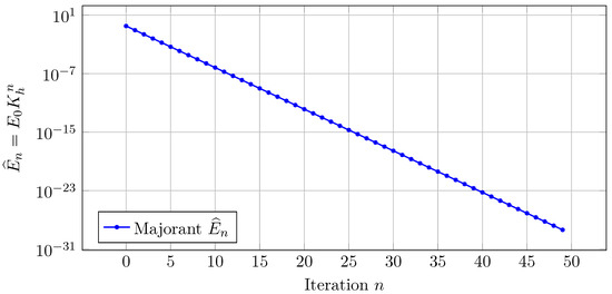
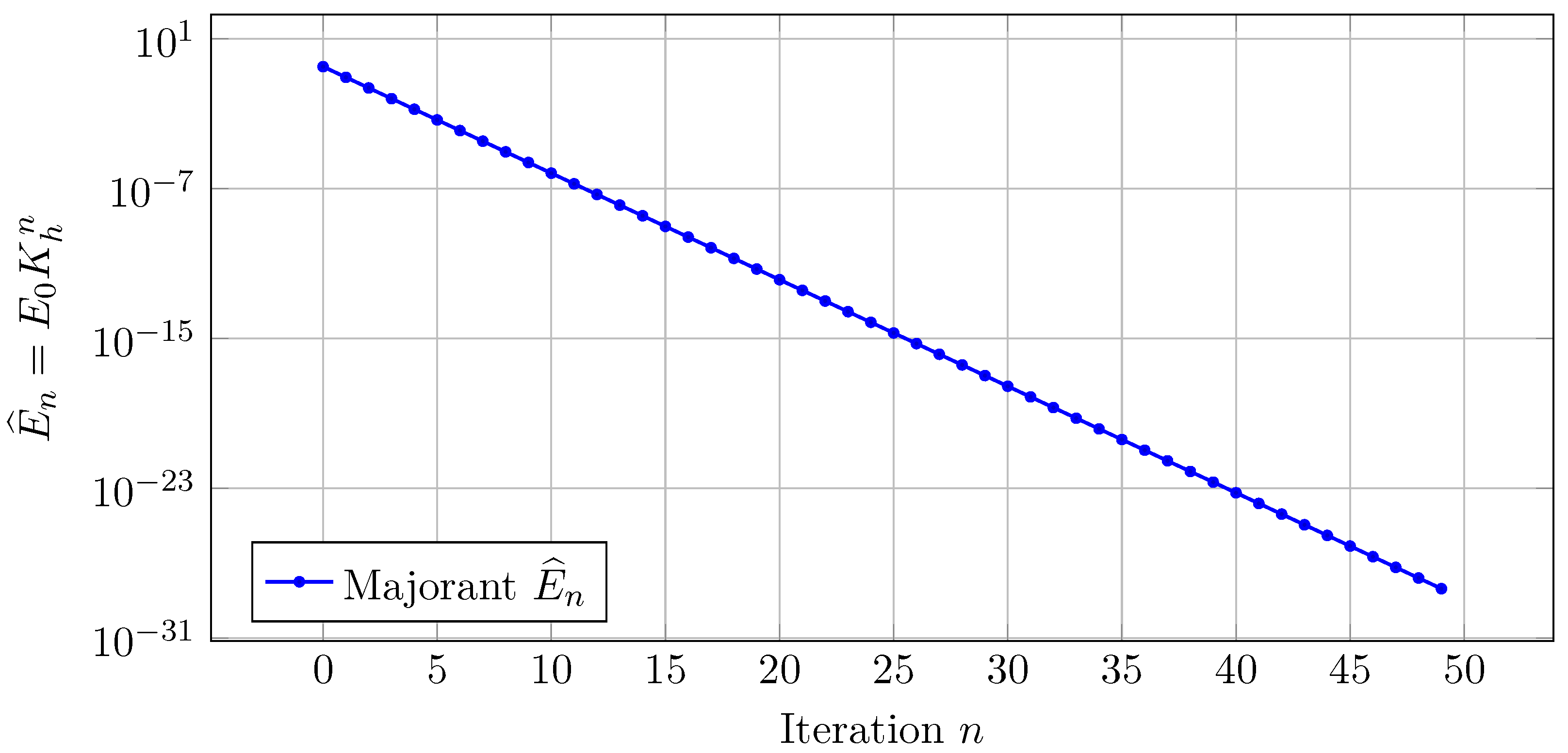
To visualise the geometric decay of the majorant, we plot ${\widehat{E}}_n$ on a semi-logarithmic scale. Figure 6 shows ${\widehat{E}}_n$ as a function of the iteration index n. The straight-line behaviour is expected, since ${\widehat{E}}_n=E_0{K}_h^n$ is exactly geometric and its slope equals ${log}_{10}\left(K_h\right)$.

Figure 6. Geometric decay of the majorant ${\widehat{E}}_n=E_0{K}_h^n$ on a logarithmic scale for $0\le n\le 49$ in the fractional case.

This numerical example indicates that the rational $(a,p)-$quasicontractive framework yields not only existence and uniqueness for the Caputo problem Equation (21) but also an effective geometric control on the convergence of the natural Picard scheme.

We now give two explicit examples of data $(q,\phi ,f)$ for which all the assumptions of Theorem 3 are verified in the Caputo fractional setting. These examples are chosen so that the nonlinearity f contains a genuine delayed feedback term and satisfies a rational $(a,p)-$condition.

Example 5.

Let $\tau \in (0,\frac{1}{2})$ and fix, for definiteness,

$$\tau =0.3,\gamma =0.5,\xi =0.4,\upsilon =0.1,1<\alpha \le 2.$$

Take

$$q\left(t\right):=1+t,t\in [0,1],$$

and prescribe the history

$$\phi \left(t\right):=1+t+\tau ,-\tau \le t\le 0.$$

For the delayed nonlinearity, we choose

$$f(t,\psi ):=\lambda {\displaystyle \frac{\psi \left(0\right)+\psi (-\tau )}{1+{\left|\psi \left(0\right)-\psi (-\tau )\right|}^p}},t\in [0,1],\psi \in C\left([-\tau ,0]\right),$$

(54)

with parameters $p\in \mathbb{N}$ and $0<\lambda <1$ to be specified below.

Since q and φ are continuous on their respective domains, Equation (22), that is, continuity and positivity of the data, is satisfied. The mapping $\psi \mapsto f(t,\psi )$ is continuous on $C\left(\right[-\tau ,0\left]\right)$ for each t, and

$$\left|f(t,\psi )\right|\le \lambda {\displaystyle \frac{\left|\psi \right(0\left)\right|+\left|\psi \right(-\tau \left)\right|}{1}}\le 2\lambda {\parallel \psi \parallel }_{\infty },$$

so (H1) holds with a linear growth bound depending only on λ. Moreover, for any $\psi ,\chi \in C\left(\right[-\tau ,0\left]\right)$ we have

$$\begin{array}{cc}\hfill & \left|f(t,\psi )-f(t,\chi )\right|\hfill \\ \hfill & \le \lambda \left|{\displaystyle \frac{\psi \left(0\right)+\psi (-\tau )}{{1+|\psi \left(0\right)-\psi (-\tau )|}^p}}-{\displaystyle \frac{\chi \left(0\right)+\chi (-\tau )}{{1+|\chi \left(0\right)-\chi (-\tau )|}^p}}\right|\hfill \\ \hfill & \le 2\lambda {\displaystyle \frac{\left|\psi \left(0\right)-\chi \left(0\right)\right|+\left|\psi (-\tau )-\chi (-\tau )\right|}{1+{\left|\psi \left(0\right)-\chi \left(0\right)\right|}^p+{\left|\psi (-\tau )-\chi (-\tau )\right|}^p}}\hfill \\ \hfill & \le 4\lambda {\displaystyle \frac{{\parallel \psi -\chi \parallel }_{\infty }}{{1+\parallel \psi -\chi \parallel }_{\infty }^p}}.\hfill \end{array}$$

Thus (H2) is satisfied with a rational Lipschitz bound of the form

$$\left|f(t,\psi )-f(t,\chi )\right|\le L_f{\phi }_p\left({\parallel \psi -\chi \parallel }_{\infty }\right),L_f:=4\lambda ,$$

where ${\phi }_p\left(r\right):=r/(1+r^p)$.

We next compute ${\Theta }_p$. By Lemma 4, the Hammerstein operator T associated with Equation (54) satisfies

$$d^p(Tx,Ty)\le {\Theta }_p{\phi }_p\left(d(x,y)\right),x,y\in C_R,$$

with

$${\Theta }_p:=L_f^p{\left(\underset{t\in [0,1]}{sup}{\int }_0^1|G_{\alpha }(t,\rho )\left|\right|q\left(\rho \right)|d\rho \right)}^p.$$

(55)

Since $G_{\alpha }$ is continuous on ${[0,1]}^2$ and $q\left(t\right)=1+t$ is bounded by 2, the supremum in Equation (55) is finite, denote it by $C_G>0$. Hence,

$${\Theta }_p\le {\left(4\lambda C_G\right)}^p.$$

Choosing, for instance,

$$\lambda :={\displaystyle \frac{1}{8C_G}},$$

we obtain

$${\Theta }_p\le {\left({\displaystyle \frac{1}{2}}\right)}^p<1,$$

so the smallness condition Equation (35) holds.

Let $R>0$ be any radius satisfying the invariance condition Equation (31). Then all assumptions of Theorem 3 are fulfilled. Consequently, the fractional boundary value problem Equation (21) with the data $q,\phi ,f$ given above has a unique positive solution ${\nu }^{*}\in P$, and for every initial guess $x_0\in C_R$ the Picard iteration $x_{n+1}:=T{x}_n$ converges in X to the associated fixed point $x^{*}$, whose extension ${\nu }^{*}$ solves Equation (21).

Example 6.

We now consider a slightly different nonlinearity, combining a logistic reaction with a delayed feedback. Fix parameters

$$\tau =0.25,\delta >0,0<\lambda <1,c>0,p\in \mathbb{N},1<\alpha \le 2.$$

Let

$$q\left(t\right):=1,\phi \left(t\right):=1.2,-\tau \le t\le 0,$$

and define

$$f(t,\psi ):=\lambda {\displaystyle \frac{\psi \left(0\right)\left(1-\psi \left(0\right)/\delta \right)+c\psi (-\tau )}{1+{\left|\psi \left(0\right)-\psi (-\tau )\right|}^p}},t\in [0,1],\psi \in C\left([-\tau ,0]\right).$$

(56)

As in Example 5, the mapping f is continuous in both variables and satisfies a rational Lipschitz condition on bounded sets. Indeed, writing ${\psi }_0:=\psi \left(0\right)$ and ${\psi }_{-\tau }:=\psi (-\tau )$, we have

$$\left|{\psi }_0(1-{\psi }_0/\delta )-{\chi }_0(1-{\chi }_0/\delta )\right|\le C_{\delta }|{\psi }_0-{\chi }_0|,$$

with $C_{\delta }:=1+2R/\delta$ on the bounded set $C_R$, while $|{\psi }_{-\tau }-{\chi }_{-\tau }{|\le \parallel \psi -\chi \parallel }_{\infty }$. A standard estimate yields

$$\left|f(t,\psi )-f(t,\chi )\right|\le L_{\delta ,c,\lambda }{\displaystyle \frac{{\parallel \psi -\chi \parallel }_{\infty }}{{1+\parallel \psi -\chi \parallel }_{\infty }^p}}=L_{\delta ,c,\lambda }{\phi }_p\left({\parallel \psi -\chi \parallel }_{\infty }\right),$$

for some constant $L_{\delta ,c,\lambda }>0$ depending only on $\delta ,c$, λ and R. Therefore, (H2) holds again.

The growth condition (H1) follows from the polynomial structure of Equation (56): on $C_R$ we have

$$\left|f(t,\psi )\right|\le \lambda {\displaystyle \frac{|{\psi }_0|+|{\psi }_0{|}^2/\delta +c\left|{\psi }_{-\tau }\right|}{1}}\le C_R{(1+\parallel \psi \parallel }_{\infty }),$$

for a suitable constant $C_R>0$. Hence, the same argument as in Example 5 gives

$$d^p(Tx,Ty)\le {\Theta }_p{\phi }_p\left(d(x,y)\right),{\Theta }_p\le {\left(L_{\delta ,c,\lambda }{C}_G\right)}^p,$$

where $C_G$ is as in Equation (55). Choosing λ small enough so that $L_{\delta ,c,\lambda }{C}_G<1$, we again obtain ${\Theta }_p<1$.

It follows that for these data, the Hammerstein operator T is a strict rational $(a,p)-$quasicontr- action on $C_R$, Theorem 3 applies, and the delayed fractional nonlocal boundary value problem Equation (21) admits a unique positive solution ${\nu }^{*}\in P$ obtained as the limit of the Picard iteration.

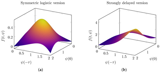
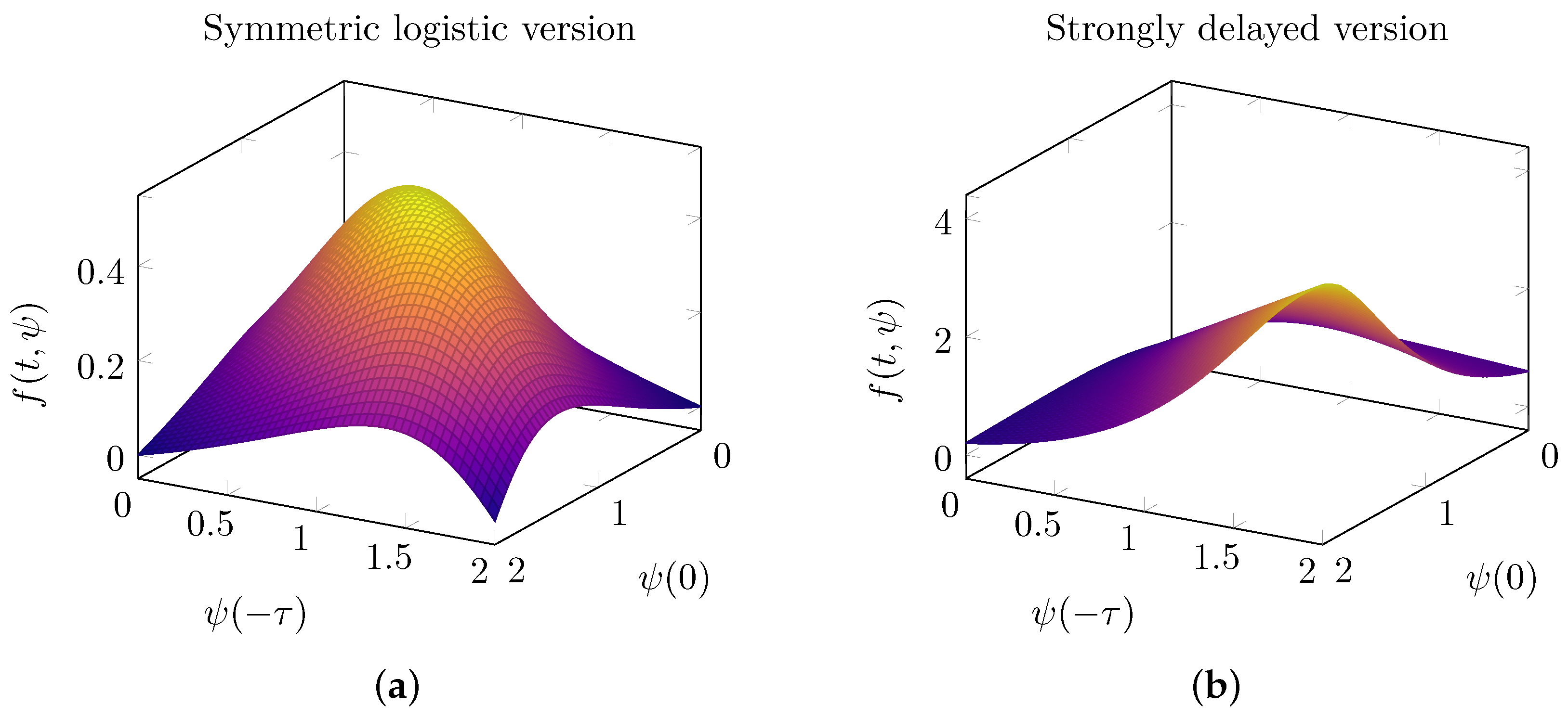
The values $\lambda =0.5$, $\delta =2$, $p=2$, and $c=3$ used in Figure 7 were chosen as a representative, moderate parameter set that yields clearly distinguishable surfaces on the visualization window $[0,2]\times [0,2]$ and illustrates two qualitatively different delayed responses, such as symmetric and delay-dominated.

Figure 7. Comparison of two delayed nonlinearities as functions of $\psi \left(0\right)$ and $\psi (-\tau )$: (a) a symmetric logistic variant $f_{\mathrm{sym}}$ and (b) a delay–dominated variant $f_{\mathrm{delay}}$, illustrated with parameters $\lambda =0.5$, $\delta =2$, $p=2$ and $c=3$.

The roles of the parameters can be explained as follows:

i. 

λ is an overall gain parameter: increasing λ increases the Lipschitz factor in (H2) and therefore enlarges the sufficient admissibility constant ${\Theta }_p$.

ii. 

δ, the logistic scale, carrying capacity, controls the curvature and saturation level of the logistic term; $\delta =2$ matches the plotting domain $[0,2]$ and yields a bell-shaped profile in the symmetric case.

iii. 

p controls the strength of the rational normalisation ${1+|\psi \left(0\right)-\psi (-\tau )|}^p$: larger p suppresses off-diagonal behaviour more strongly.

iv. 

c weights the delayed contribution $\psi (-\tau )$; larger c increases the influence of the past state and produces a more anisotropic surface.

If λ and/or c are increased substantially, then the constant $L_{\delta ,c,\lambda }$ in (H2) grows, at least linearly, and the sufficient smallness condition ${\Theta }_p<1$ may fail. In that area, the operator may no longer be a strict rational $(a,p)-$quasicontraction, so the Picard iteration may converge more slowly or lose global contractive behaviour. Conversely, decreasing λ or choosing a smaller c strengthens the contraction effect and speeds up convergence. Changing δ mainly reshapes the logistic curvature, while changing p modifies how strongly discrepancies away from $\psi \left(0\right)\approx \psi (-\tau )$ are penalised.

The figure illustrates the qualitative behaviour of the two delayed nonlinearities. In the left panel, the symmetric logistic variant exhibits a smooth bell-shaped surface and remains uniformly bounded on $[0,2]\times [0,2]$, while the rational normalisation $1+{|\psi \left(0\right)-\psi (-\tau )|}^p$ suppresses the response away from the diagonal. In contrast, the right panel shows a delay-dominated response: the weight $c>1$ in front of $\psi (-\tau )$ produces a much steeper growth in the $\psi (-\tau )-$direction, so that large values of the past state have a stronger impact on $f(t,\psi )$ than the instantaneous value $\psi \left(0\right)$.

5. Conclusions

In this paper, we have introduced and analysed a bounded rational normalisation of the Popescu-Stan $(a,p)-$framework, leading to the notions of rational $(a,p)-$quasicontractions on metric and Banach spaces. By replacing the unbounded interpoint block $d^p(x,y)$ with its bounded counterpart

$${\varphi }_p\left(d(x,y)\right):={\displaystyle \frac{d^p(x,y)}{1+d^p(x,y)}},$$

we obtained Greguš-type fixed point theorems on compact metric spaces and on closed, convex subsets of Banach spaces under relative compactness assumptions on the range of the operator. In all cases, we proved the existence and uniqueness of fixed points, as well as the global convergence of the Picard iteration for every initial guess. Several discontinuous examples on $[-1,1]$ demonstrate that rational classes strictly extend the classical Hardy–Rogers, Kannan, Chatterjea and rational contractions, thereby clarifying the position of our framework in the landscape of nonlinear contractive mappings.

The second main contribution concerns an application to a delayed multi-point Caputo fractional boundary value problem with nonlocal conditions. We considered a Caputo problem of order $\alpha \in (1,2)$ with distributed delay and mixed multi-point boundary conditions, derived the associated fractional Green kernel, and obtained two-sided bounds that allow the construction of an invariant cone–ball $C_R\subset X=C([-\tau ,1],\mathbb{R})$. Under natural growth and rational Lipschitz assumptions on delayed nonlinearity, we showed that the corresponding Hammerstein-Volterra operator $T:C_R\to C_R$ is a strict rational $(a,p)-$quasicontraction with relatively compact range. The abstract theory then yields the existence and uniqueness of a positive solution in the cone, together with the global attractivity of this solution under the Picard iteration.

Finally, we presented a numerical scheme based on a collocation discretisation of the fractional Hammerstein equation, and we illustrated the predicted geometrically fast convergence of the discrete Picard iteration in representative delayed fractional models. The numerical error history confirms the rational $(a,p)-$quasicontractive behaviour of the Hammerstein operator and highlights the practical advantages of rational normalisation on large scales.

Despite the breadth of the rational normalisation approach, several critical points deserve emphasis. First, the abstract fixed point results rely on compactness or relative compactness of the range; extending the theory to noncompact settings, for instance, by using measures of noncompactness or alternative compactness surrogates would significantly widen its functional-analytic reach. Second, in the fractional application the key admissibility requirements in particular the invariance condition $MB<1$ and the strictness threshold ${\Theta }_p<1$ tie the applicability of the method to quantitative bounds on the Green kernel and to growth/Lipschitz data of the nonlinearity; obtaining sharper two-sided Green estimates and less conservative constants is therefore central, especially near the borderline regime ${\Theta }_p\uparrow 1$. Third, while the numerical illustration exhibits a rapidly stabilising geometric factor, a systematic continuous-discrete consistency analysis remains open: one would like explicitly a priori bounds relating the discrete convergence factor of the collocation scheme to the continuous constants $(B,{\Theta }_p)$, including mesh dependence and stability of the discrete Picard operator. Finally, the present delayed Caputo example uses a comparatively tractable feedback structure; treating genuinely state-dependent delays, multi-term Caputo dynamics, or variable-order kernels within the same rational $(a,p)-$framework is expected to require new technical ideas.

Several directions for future research emerge from this work. On the abstract side, it would be natural to investigate vector-valued and set-valued extensions of rational $(a,p)-$quasicontractions, as well as variable-order or nonlocal-in-time versions adapted to fractional operators with memory. On the applied side, our framework can be combined with more complex fractional models, such as systems of Caputo equations with impulsive or stochastic perturbations, as well as nonlocal problems posed on irregular or fractal-type spatial domains. These developments will be pursued in forthcoming work.

References

- Banach, S. Sur les opérations dans les ensembles abstraits et leur application aux équations intégrales. Fundam. Math. 1922, 3, 133–181. [Google Scholar] [CrossRef] [Scilit]
- Kannan, R. Some results on fixed points. Bull. Calcutta Math. Soc. 1968, 60, 71–76. [Google Scholar]
- Chatterjea, S.K. Fixed point theorems. C. R. Acad. Bulgare Sci. 1972, 25, 727–730. [Google Scholar] [CrossRef] [Scilit]
- Hardy, G.E.; Rogers, T.D. A generalization of a fixed point theorem of Reich. Canad. Math. Bull. 1973, 16, 201–206. [Google Scholar] [CrossRef] [Scilit]
- Edelstein, M. On fixed and periodic points under contractive mappings. J. Lond. Math. Soc. 1962, 37, 74–79. [Google Scholar] [CrossRef] [Scilit]
- Meir, A.; Keeler, E. A theorem on contraction mappings. J. Math. Anal. Appl. 1969, 28, 326–329. [Google Scholar] [CrossRef] [Scilit]
- Greguš, M. A fixed point theorem in Banach spaces. Boll. Un. Mat. Ital. 1980, 5, 193–198. [Google Scholar]
- Popescu, O.; Stan, G. Some fixed point theorems for (a, p)−quasicontractions. Symmetry 2020, 12, 1973. [Google Scholar] [CrossRef] [Scilit]
- Popescu, O.; Stan, G. Some fixed point theorems for quadratic quasicontractive mappings. Symmetry 2019, 11, 1329. [Google Scholar] [CrossRef] [Scilit]
- Girgin, E.; Büyükkaya, A.; Kuru, N.K.; Younis, M.; Öztürk, M. Analysis of Caputo-Type Nonlinear Fractional Differential Equations and Their Ulam–Hyers Stability. Fractal Fract. 2024, 8, 558. [Google Scholar] [CrossRef] [Scilit]
- Büyükkaya, A.; Kesik, D.; Yeşil, Ü.; Öztürk, M. New Studies for Dynamic Programming and Fractional Differential Equations in Partial Modular b-Metric Spaces. Fractal Fract. 2024, 8, 724. [Google Scholar] [CrossRef] [Scilit]
- Yeşil, Ü.; Aydin Akgun, F.; Öztürk, M.; Rasulov, Z. A New Approach for the Solution of Fourth-Order Boundary Value Problems. J. Integral Equ. Appl. 2025, 37, 247–254. [Google Scholar] [CrossRef] [Scilit]
- Wang, P.; Han, B.; Bao, J. The Ulam Stability of High-Order Variable-Order φ-Hilfer Fractional Implicit Integro-Differential Equations. Fractal Fract. 2024, 8, 502. [Google Scholar] [CrossRef] [Scilit]
- Hafeez, F.; Jeelani, M.B.; Alhamzi, G. Fractional-Order Delay Differential Equations: Existence, Uniqueness, and Ulam–Hyers Stability. Axioms 2025, 14, 817. [Google Scholar] [CrossRef] [Scilit]
- Aljoudi, S.; Alamri, H.; Alrubaie, M. Study of a Coupled System of Integro-Differential Equations Involving the Generalized Proportional Caputo Derivatives. Fractal Fract. 2025, 9, 735. [Google Scholar] [CrossRef] [Scilit]
- Esloub, S.; Alhazzani, E.; Gadain, H.E. A Two-Dimensional Nonlocal Fractional Parabolic Initial Boundary Value Problem. Axioms 2024, 13, 646. [Google Scholar] [CrossRef] [Scilit]
- Dass, B.K.; Gupta, S. An extension of Banach contraction principle through rational expression. Indian J. Pure Appl. Math. 1975, 6, 1455–1458. [Google Scholar]
- Jaggi, D.S. Some unique fixed point theorems. Indian J. Pure Appl. Math. 1977, 8, 223–230. [Google Scholar]
- Hacini, M.e.M.; Djilali, S.; Zeb, A.; Gul, N.; Saeed, T. Existence and multiplicity of positive solutions for a second order multi-point delayed boundary value problem. Results Phys. 2022, 40, 105865. [Google Scholar] [CrossRef] [Scilit]
Disclaimer/Publisher’s Note: The statements, opinions and data contained in all publications are solely those of the individual author(s) and contributor(s) and not of MDPI and/or the editor(s). MDPI and/or the editor(s) disclaim responsibility for any injury to people or property resulting from any ideas, methods, instructions or products referred to in the content. |
© 2026 by the author. Licensee MDPI, Basel, Switzerland. This article is an open access article distributed under the terms and conditions of the Creative Commons Attribution (CC BY) license.