


Abstract
This paper proposes a rotation-locking alignment scheme and system based on a Gaussian beam addressing the relative displacement between the receiver and the spot center during the fine tracking phase of spaceborne laser communication APT technology caused by platform vibration, temperature variations and other factors. By rotational scanning fitting, the offset angle and offset distance of the receiver relative to the spot center can be derived and achieve high-precision adaptive tracking. The simulated result demonstrates that the fitting distance error of this scheme is less than 1%, and the fitting angle error is less than π/32. At the same time, the system prototype is developed to conduct ground-based validation experiments, including the static test and outdoor link establishment test. The system prototype features simpler structure, lower computational complexity, and easier integration, satisfying the miniaturization and lightweight design requirements for spaceborne laser communication terminals. The test results verify the system can successfully establish stable laser communication links rapidly.
1. Introduction
With the development of modern space–air–ground information networks, traditional microwave satellite communication technology is gradually struggling to meet the demands of high-capacity, high-speed data transmission. Moreover, microwave communication terminals are characterized by significant mass and volume, which increase system power consumption and the load on satellite platforms. In contrast, laser communication technology offers advantages such as strong confidentiality, high data transmission rates, and compact terminal sizes [1,2,3,4,5,6]. Consequently, spaceborne laser communication technology holds broad application prospects and significant development potential for next-generation satellite communication networks. Internationally, extensive verification research has been conducted on related theories and experimental apparatus [7,8,9,10,11,12,13,14].
In spaceborne laser communication technology, due to the extremely small divergence angle of laser beams, communication terminals require exceptionally high pointing alignment accuracy to achieve continuous and reliable communication. The acquisition, pointing, and tracking (APT) technology is one of the key technologies for establishing stable and aligned laser communication links by rapidly acquiring the optical signal within an initial uncertainty area with high precision and achieving tracking to ensure efficient coupling of the optical signal into the receiving fiber [15,16,17,18]. To guarantee alignment efficiency and accuracy, APT systems typically employ a composite control structure comprising coarse tracking and fine tracking [19,20]. The coarse tracking system is used to acquire the approximate position of the beam on the receiver, while the fine tracking system further corrects the position offset caused by satellite platform vibration, temperature variations, or other factors, to improve beam alignment accuracy.
This paper proposes a novel rotation-locking scheme and algorithm based on Gaussian beams aimed at the miniaturization and lightweight requirements of spaceborne laser communication APT systems, which can calculate the relative distance offset and angle offset between the spot position and the receiver to achieve alignment and tracking through a fitting algorithm. The simulation result indicates that the fitting algorithm achieves a distance error of less than 1% and an angle error of less than π/32. The specific computation is implemented on Field Programmable Gate Array (FPGA), and the prototype testing system is designed to verify the feasibility of the algorithm. Through ground tests, the system successfully achieves adaptive alignment and link establishment. Compared with traditional fine-tracking schemes, its core advantage is no need for complex systems and beacon-assisted optical paths and lower computational complexity and resource occupation, which is suitable for low-cost, miniaturized, lightweight spaceborne terminals with SWaP (Size, Weight, and Power) constraints.
2. Materials and Methods
During the fine tracking process of laser communication, various factors cause relative displacement between the optical receiver and the received spot, such as vibration-induced deformation of the mechanical structure and temperature variations. This prevents precise alignment between the transmitting laser signal and the receiver, thereby degrading communication quality. This paper proposes a rotation-locking fitting algorithm based on a Gaussian beam model by transforming the Gaussian intensity distribution into linear equation form and applying the least squares method to analyze the collected intensity and obtain a regression line. In this way, the angle offset φ and distance offset d between the receiver and the spot center can be calculated to achieve accurate tracking. The specific algorithm principle and calculation process is described below.
2.1. Materials
Based on the Gaussian intensity distribution model, the system takes the coordinate of the received cumulative spot center as the center of a scan circle and controls a laser signal to perform equally spaced rotational scanning along the circular path. When the scanning spot center positions at different locations, the receiver correspondingly collects the optical signal intensity from each scan to fit the angle offset and distance offset .
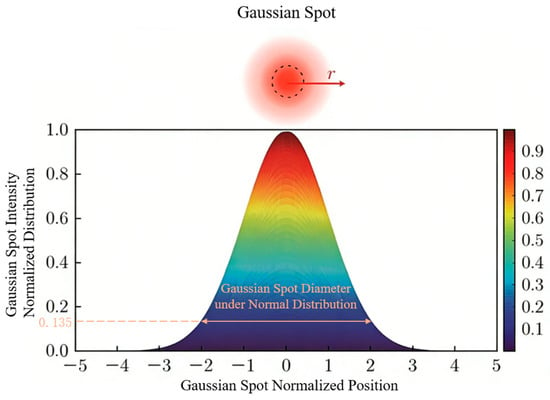
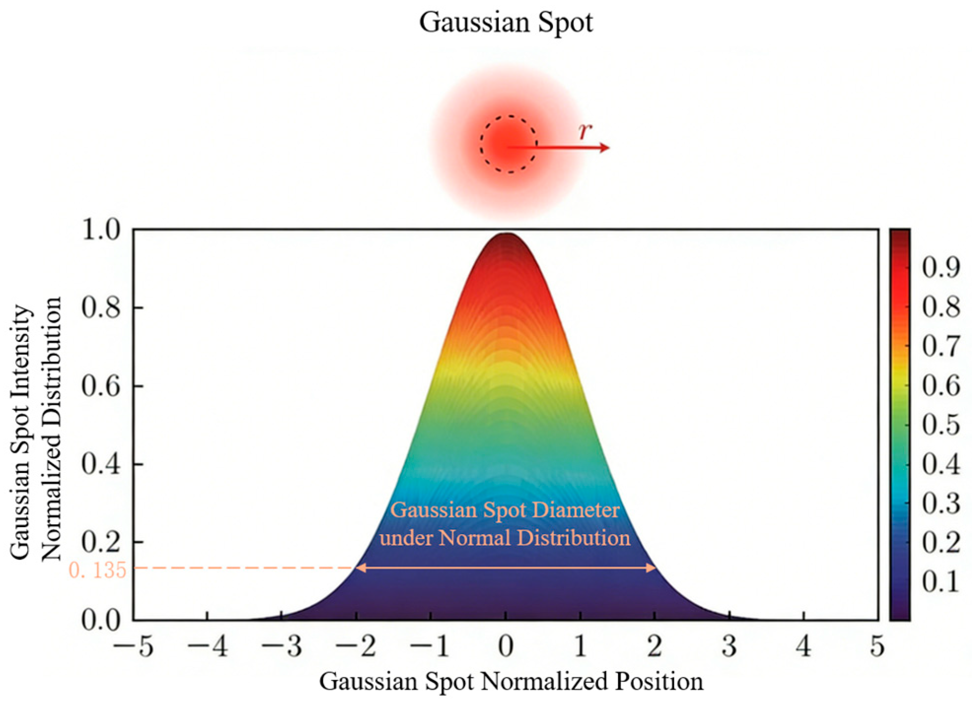
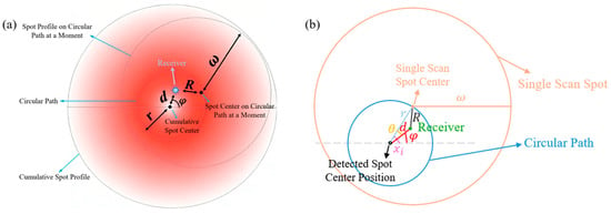
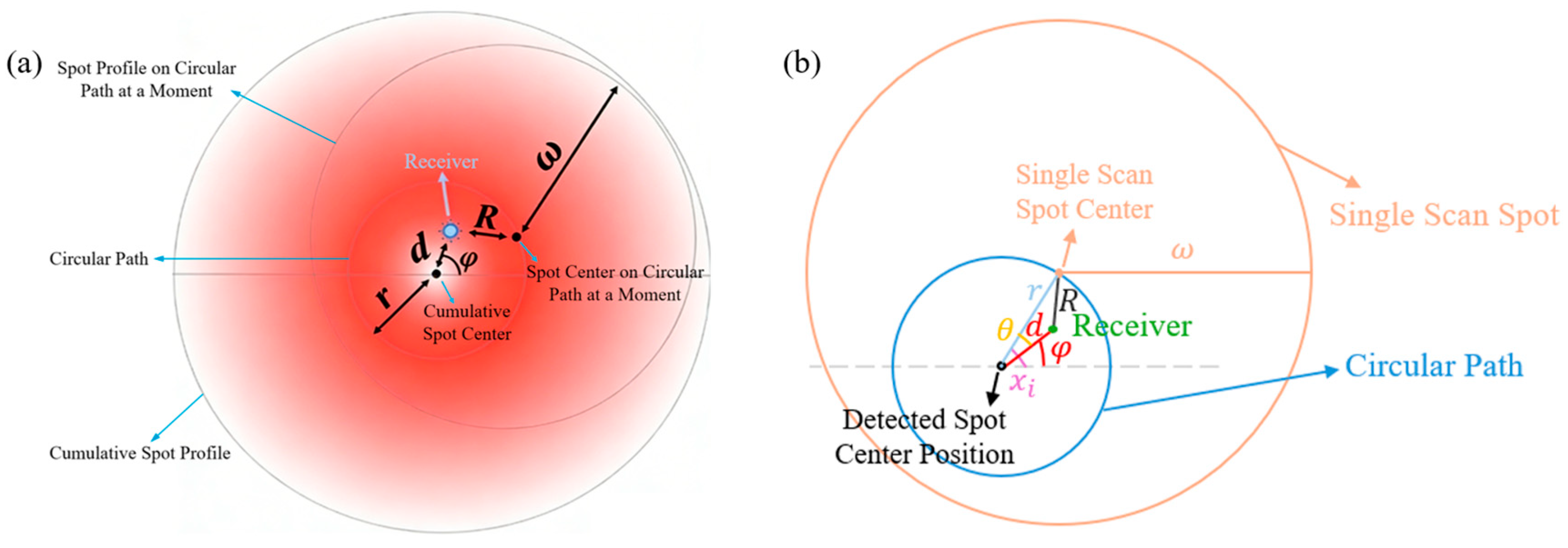
Figure 1 shows the Gaussian intensity distribution of the laser signal [21,22], and Figure 2a shows the rotational scanning principle at a specific moment, including the positions of cumulative spot center and profile, circular path, the momentary scanning spot center and profile, as well as the receiver. It can be observed that there is an angle offset and a distance offset d between the receiver and the cumulative spot center. The center of a circular path is found using the coordinates of a cumulative spot center detected by coarse tracking. The scanning laser signal is controlled to rotate along the circular path of radius r at equal intervals. Figure 2b presents a simplified model, where represents the scan angle for the i-th scan.
Figure 1.
Schematic diagram of ideal Gaussian intensity distribution: the dashed circle represents the waist radius of the Gaussian spot.
Figure 2.
The position of spot and receiver in rotational scanning principle at a specific moment: (a) specific spot model; (b) simplify mathematical model.
Assuming the power of a scanning laser is and its spot radius is , the scanning optical intensity collected by the receiver at its location shown in Figure 2b can be expressed as
where S is the spot area, and R is the distance between the receiver and the single scanning spot center, which can be expressed as
where .
The optical intensity can be also expressed as
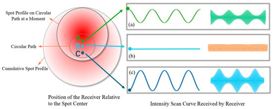
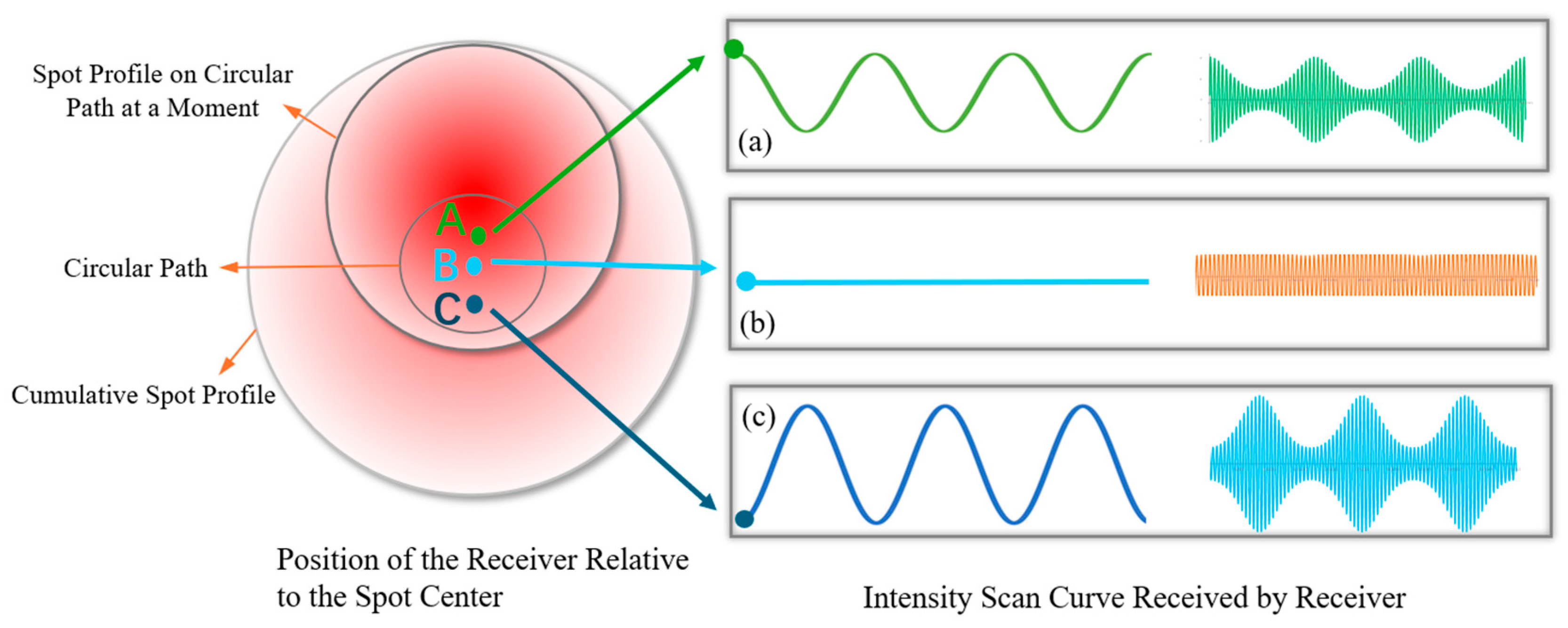
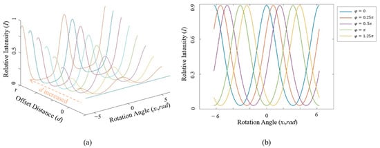
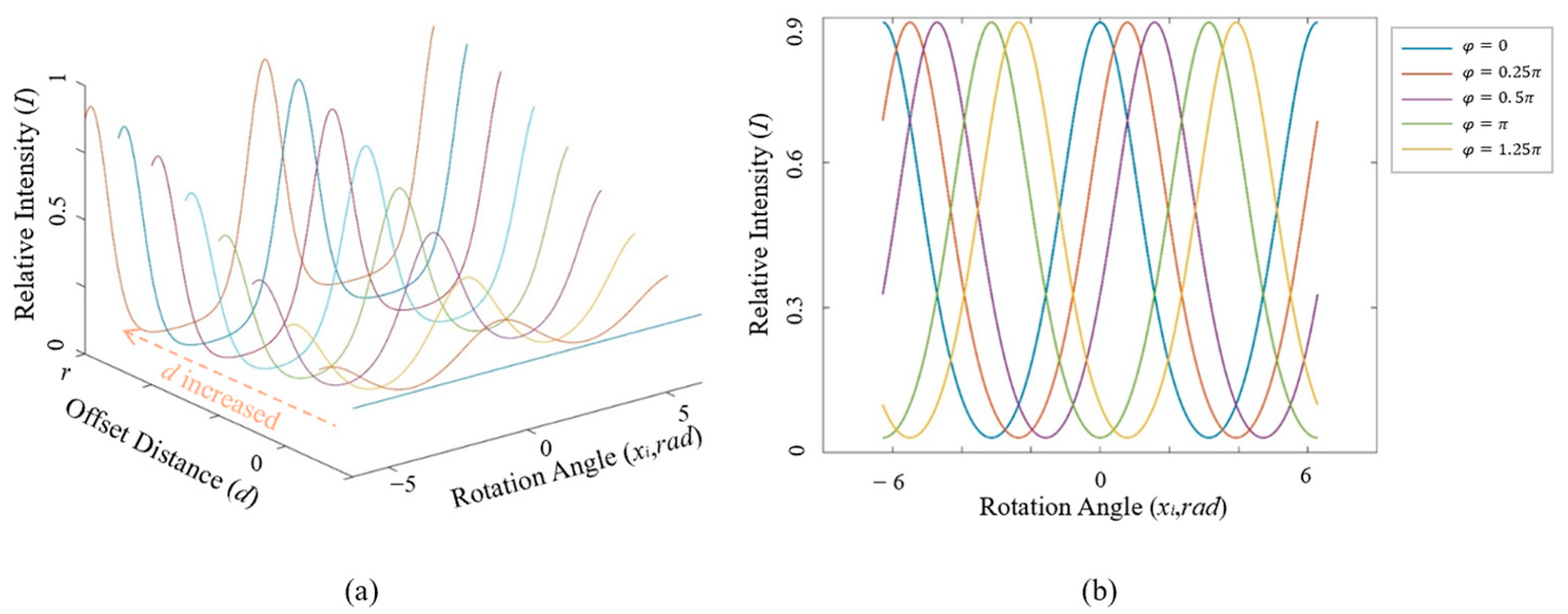
According to this equation, the intensity scan curve at the receiver (variation in scanning intensity with scan angle ) when the receiver is positioned at different locations relative to the cumulative spot center is shown in Figure 3. Point B in Figure 3 represents the receiver located on the cumulative spot center, where and . And the points A and C represent the receiver being located above and below the cumulative spot center. As and vary, the amplitude and phase of intensity scan curves are different. When the receiver is on point B, the collected signal almost remains constant at each scanning point, and the intensity scan curve of optical intensity and scanning angle seems a straight line (as in Figure 3b), which means the link is in the aligned state. Figure 4 further illustrates the variation trend of the intensity scan curve with offset angle and offset distance. When keeps constant, the amplitude fluctuation of the intensity scan curve increases as increases. When keeps constant, the phase of the intensity scan curve changes correspondingly with . Therefore, and can be fitted from the intensity scan curve.
Figure 3.
Intensity scan curves when the receiver is at different positions relative to the cumulative spot center: (a) the receiver located on point A; (b) the receiver located on point B; (c) the receiver located on point C.
Figure 4.
Variation trend of the ideal optical intensity curve with and : (a) relative intensity curve with different offset distance; (b) relative intensity curve with different offset angle.
In FPGA, solving complex exponential functions consumes significant resources, difficult to implement in engineering. To simplify the calculation of and from Equation (3) with complex functions, take the logarithm of both sides:
Assuming , , the above equation can be expressed as
Thus, it transforms the complex function operation into a linear fitting process of InI and , simplifying the computational process and reducing the computational load.
2.2. Calculation Method of
According to the expression of parameter B, B > 0, it can be learned that the closer the value of approaches zero, the greater the received optical intensity I becomes. Therefore, by finding the maximum value and the second maximum value of the scanning intensity and their corresponding scan angles, an approximate value approaching can be obtained. Then, the offset distance d can be calculated based on the scan points and its linear fitting relationship with substituting . Subsequently, the value of can be iterated through the estimation of d.
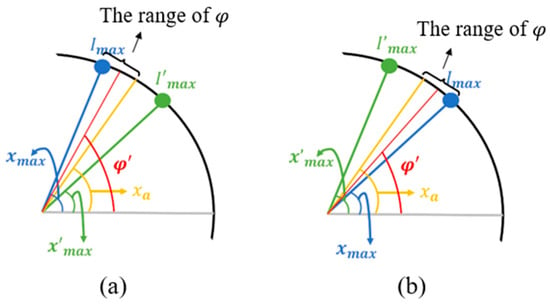
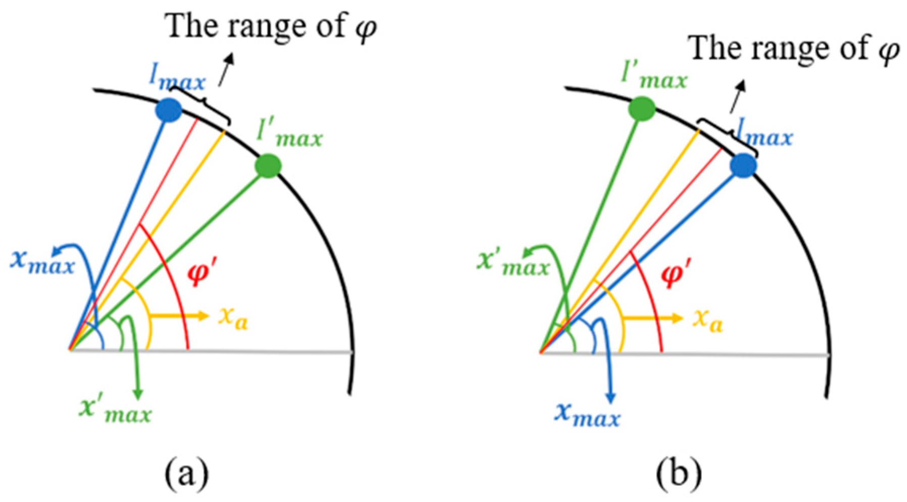
The calculation of is as follows: As the scanning spot moves at equal angular intervals along the circular path, assuming the number of scan points is N, the scan step size is 2π/N. When the scan angle of a spot more closely approaches the true offset angle of the receiver, the received optical intensity is greater. Based on the maximum value () and the second maximum value (), it can be inferred that should be closer to the maximum value . Let be the angle bisector between scan angles and be the angle bisector of and . The actual offset angle can fall into the following three cases, as shown in Figure 5:
Figure 5.
The estimated analysis of from the scanning angle of the maximum received optical intensity value and the second maximum value: (a) ; (b)
(a) When , the offset angle lies within the interval . The can be expressed as
(b) When , the offset angle lies within the interval . The can be expressed as
(c) In a special case, .
In these three cases, the error between and is less than . The number of scan points N should be selected to minimize the influence of on the offset distance estimation considering the computational load. Substituting to calculate d, the actual offset angle can be iteratively derived:
2.3. Calculation Method of d
The value of d can be calculated by fitting the optical intensity scanning curve with the least squares method. Assuming and , Equation (5) can be simplified into the linear expression
Then, the coordinate points of the scanning circle can be transformed into the corresponding coordinates for the linear expression. The least squares method fits these points to minimize the overall error for a fitted line. Through parameters A and B, the offset distance d can be solved.
The error equation of each scanning point is established as follows:
Taking the partial derivatives with respect to A and B, the equations can be obtained as follows:
The expressions for A and B are solved as follows:
Then, d can be calculated by fitting parameter B:
Based on the above theory analysis and calculation methods, the control mechanism of the rotation-locking method will be summarized further in this section. When the received optical intensity distribution conforms to the Gaussian model, the signal collected by the receiver is related to the distance between the receiver and the beam center. In the fine-tracking stage, the beam center position is obtained during the acquisition stage as the center of circular scanning, and the radius of the scanning circle is set to scan spaced evenly along the circumference. When the receiver is exactly located at the beam center, the scanning curve is a straight line. When the receiver shifts away, unless the offset angle of the receiver exactly equals the preset scanning angle, the received optical intensity varies at different scanning points due to the properties of the Gaussian distribution. The nearest scanning point to the receiver receives the strongest signal, and the signal becomes weaker as the distance increases.
From the intensity data and corresponding scanning angles, the nearest scanning angle and the distance between the receiver and the scanning spot can be fitted based on the Gaussian function, which has a triangular relationship (as Figure 2b) with the actual offset distance we need. In this way, the receiver can be localized.
3. Simulation
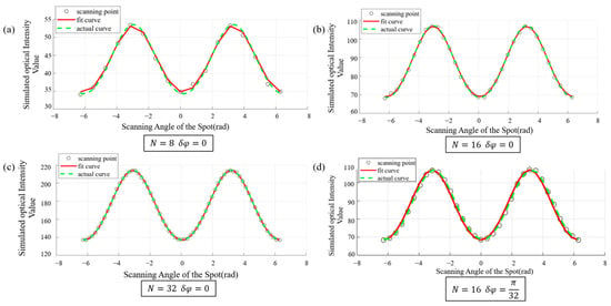
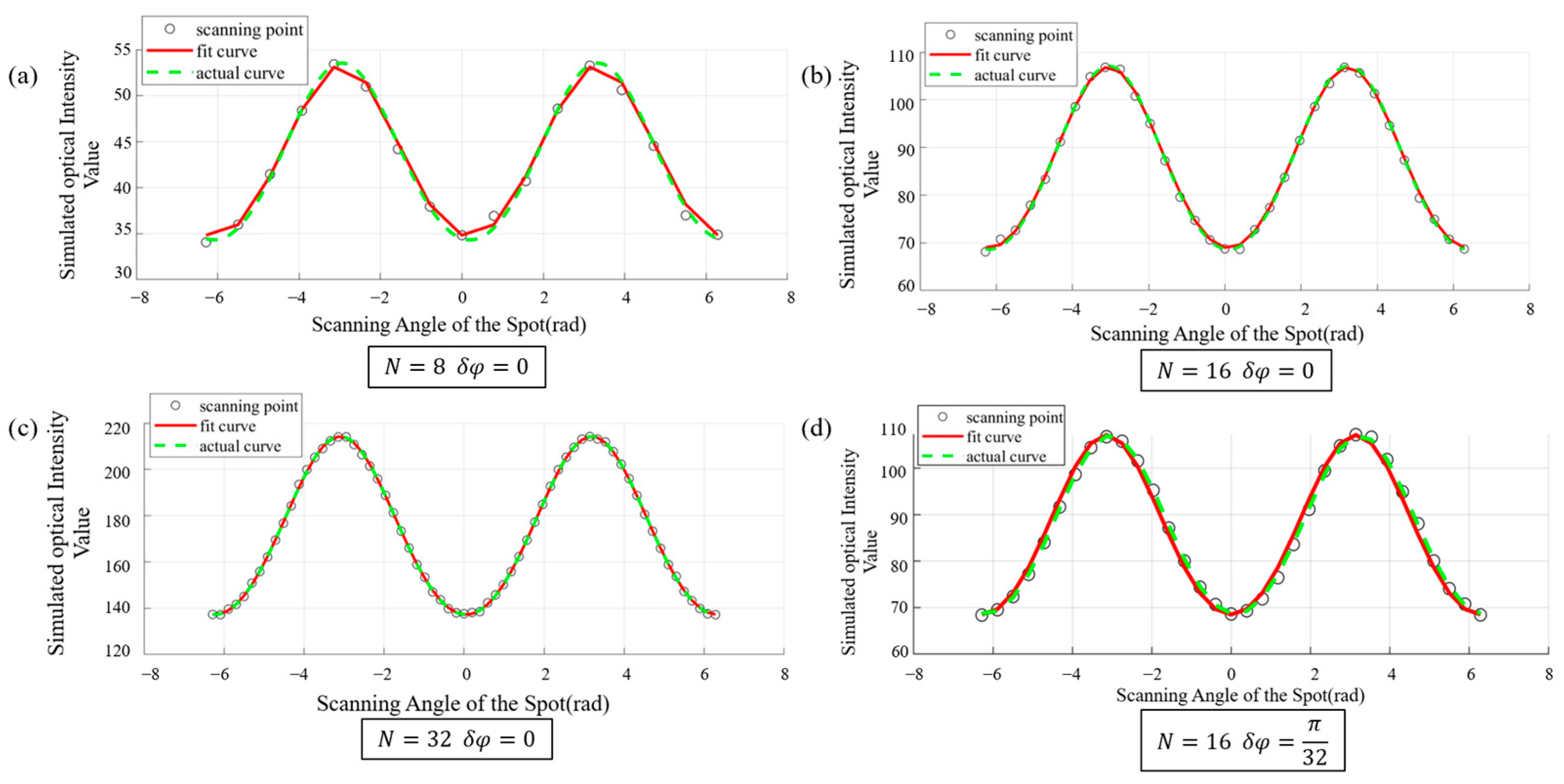
For simulation, the Gaussian beam waist radius is set to 3 mm, and the scanning circle radius is 1 mm. The additive white noise is added to simulate system noise conditions. In the calculation of , the scan points N influence the approximate value , and the error can be derived to be less than . Figure 6a–c shows the sampled points, fitted curves, and actual curves with N = 8, 16, and 32. When N = 8, the fitted curve has fewer overlapping parts with the actual curve, appearing sharp and jagged. When N = 16 and N = 32, the fitted curve becomes smoother and almost overlapped with the actual curve. Considering the computational load, N = 16 is chosen as the scan points for the system. Table 1 lists the fitting accuracy of different scanning points on the offset distance and the offset angle. Considering the fitting accuracy and computational complexity, we select N = 16 for subsequent simulations and experiments.
Figure 6.
(a–c) Fitted curves under different numbers of scan points: (a) N = 8, (b) N = 16, (c) N = 32 and offset angle error = 0. (d) The fitted curve and the actual curve when N = 16, = π/32.
Table 1.
The accuracy of N on fitting offset distance (d = 0.5) and offset angle error.
When scanning 16 points at equal intervals along the circular path, according to the calculation method of , the error is less than π/32. Figure 6d shows the sampled points, the actual curve, and the fitted curve with the maximum error value of = π/32. These curves are essentially consistent with each other, and the offset distance calculated from the fitted curve is 0.5032 with 0.64% error, less than 1% relative to the set offset distance of 0.5, indicating that when ≤ π/32, the impact of the offset angle error on offset distance calculation is small.
When the offset distance d exceeds the spot radius, the scanning spot will move outside the receiver totally at certain rotation angles during simulation. In this case, the receiver barely detects any scanning optical signal, resulting in near-zero optical power data points. And in outdoor tests, random atmospheric turbulence may cause spot wander, leading to the spot being outside the receiver. The near-zero noise detected by the receiver mainly includes background light noise and the photodetector noise. The background light noise can be largely suppressed by an optical filter. The shot noise and thermal noise power of the photodetector are of 10−24~10−22 A2/Hz normally, and dark current is about several tens of nA. The noise is approximately additive white Gaussian noise.
Due to the logarithmic operation used in linear equation conversion, the noise near zero in the received optical intensity is amplified when mapped to , leading to unsatisfactory fitting results. A threshold substitution method is adopted in the fitting algorithm. Specifically, during the measurement process, all points below a certain threshold are replaced with the minimum measured value. Through multiple fitting simulations, it acheives the best fitting performance, setting the threshold to 2.5% of the maximum value. Figure 7 illustrates the fitted curves and actual curves before and after threshold substitution when the scanned data contains values near zero. In the figure, the red dashed line represents the fitted curve, and the black dashed line represents the actual curve. It can be observed that before threshold substitution, the noise near zero significantly impacts the fitting, causing the curves to be largely misaligned. Through threshold substitution, the curve achieves better fit.
Figure 7.
Effect of noise near zero on fitting curve: (a) before threshold substitution, (b) after threshold substitution.
In spaceborne laser communication, there is no atmospheric turbulence, so the probability of near-zero data points caused by spot wander is greatly reduced. The offset distance d is a slowly varying quantity caused by environmental factors such as temperature changes, which induce a slow relative drift between the transceivers. Assuming that the acquisition and tracking module is activated once the offset distance reaches a certain level, the data points with near-zero intensity can be avoided.
Since FPGA can only use the exhaustive approach to implement division in the least squares method by using piecewise functions to represent the optical intensity values in different intervals, the exhaustive step size influences the fitting effect.
To balance fitting performance and resource utilization, we simulated the specific impact of the optical intensity value step size m on fitting performance. Figure 8a–d presents the comparison plots between the fitted curves and actual curves when m = 2, 4, 8, and 16, respectively. In these figures, the red points and curves represent the sampled values and fitted curves, while the black points and curves represent the actual intensity values and corresponding curves. As m increases, the fitted curve gradually approaches the actual curve. When m = 16, the fitted curve essentially coincides with the actual curve.
Figure 8.
The influence of optical intensity value step size on curve fitting: (a) m = 2; (b) m = 4; (c) m = 8; (d) m = 16.
To further evaluate the error of m on the fitting accuracy, Table 2 shows the fitted offset distance values d1 and their fitting errors relative to the set actual value d for different m. As m increases, the error gradually decreases. When m > 128, the fitted curve closely matches the actual curve, and the fitting error for the offset distance is less than 1%.
Table 2.
The influence of optical intensity value step size on fitting distance when d = 3.
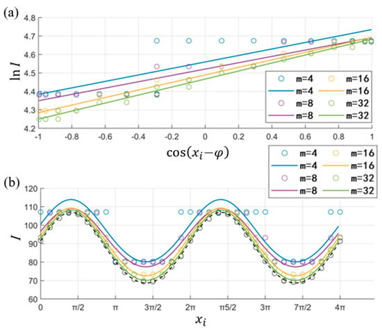
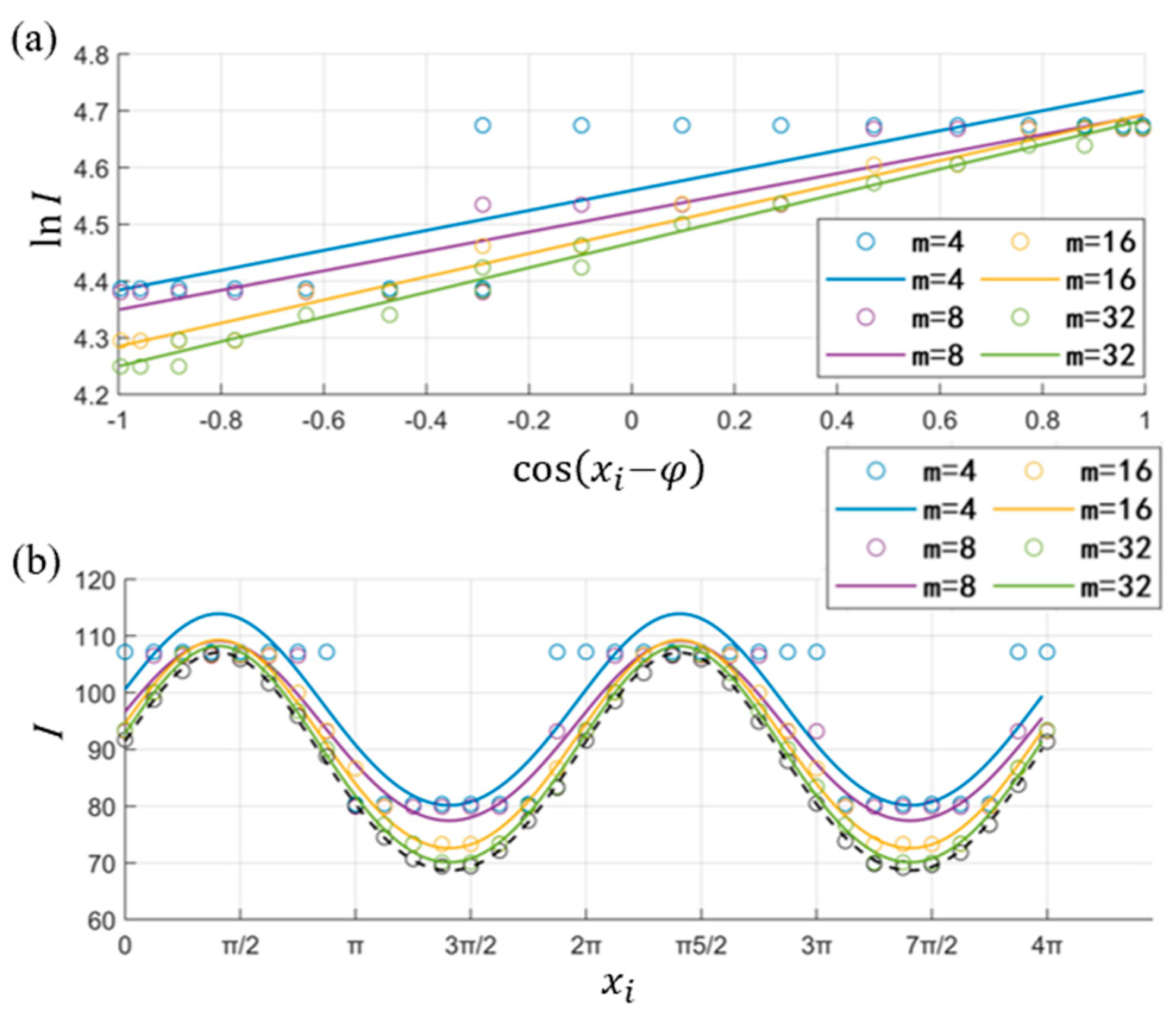
When the setting distance d is small, it is found that increasing m results in little to no change in the fitting error in Table 3. When d = 0.5 and m increases from 4 to 8, the fitting error changes very little. By fitting the regression line and the scanning curve (Figure 9), it can be observed that the regression lines for m = 4 and m = 8 are almost parallel. When using , the fitting errors are very close. The specific reason is that when d is small, the value of optical intensity is significantly greater than zero, and when the intensity value interval is divided into and equal parts for smaller m, the upper bound of the interval containing the minimum value is the same as the maximum value. After reassigning values, the maximum and minimum values used in the calculation are essentially identical.
Table 3.
The influence of optical intensity value step size on fitting distance when d = 0.5.
Figure 9.
The fitting points and curves on different optical intensity value step sizes: (a) linear regression fitting; (b) scanning curve fitting, the black dashed line and circles represent the ideal fitting curve.
During the circular spot scanning process, the received maximum and minimum powers can be expressed as
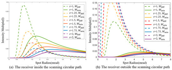
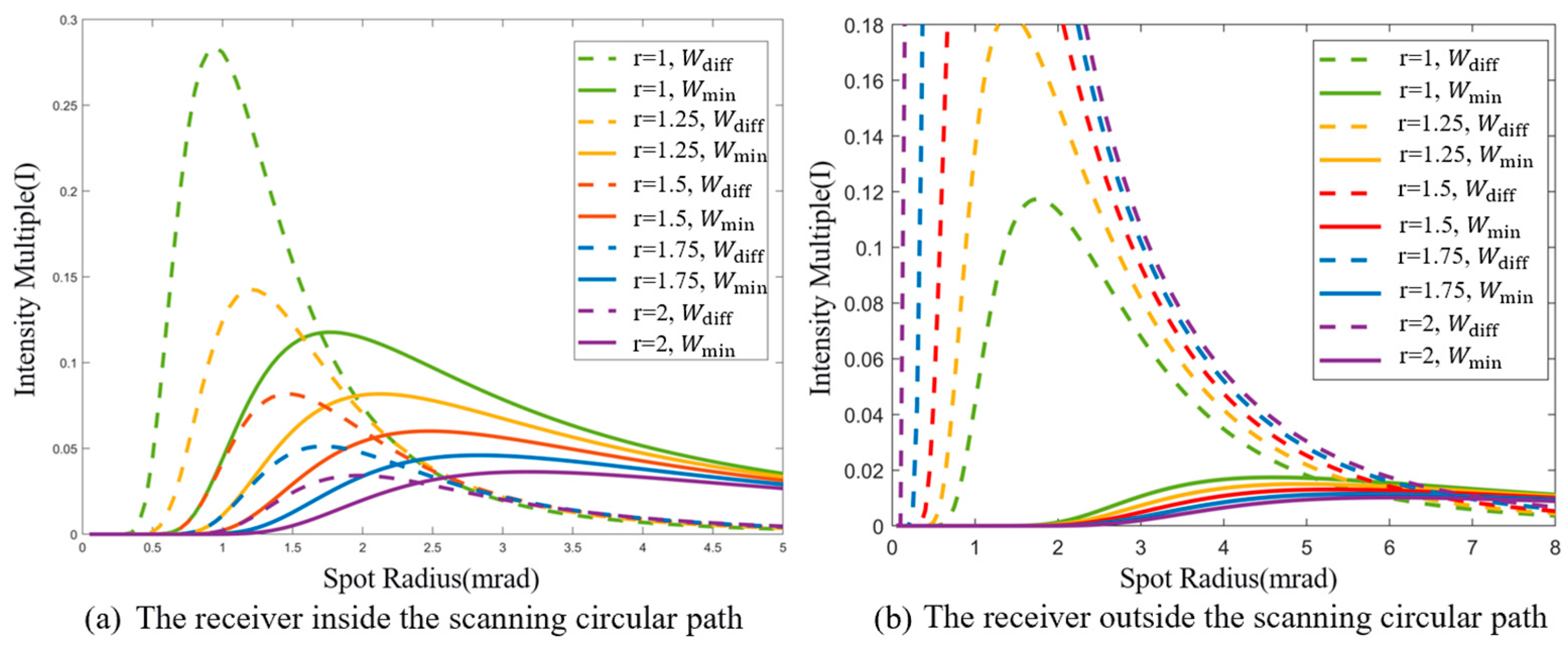
It is defined that to characterize the relative motion, with a larger Wdiff indicating a greater difference between the maximum and minimum intensities, which is beneficial for identifying the location of the strongest signal and achieving higher tracking accuracy. Meanwhile, a larger Wd,min implies higher received signal power, which means better communication quality. In specific environments, the laser power is constrained by the source while the receiver offset is influenced by the external environment. Therefore, both high tracking accuracy and good communication quality can be simultaneously achieved by optimizing the spot radius and the scanning circle radius.
Figure 10 illustrates the variation curves of tracking accuracy and communication quality with the spot radius and the scanning circle radius. The angular value is used commonly to describe lengths in practical laser communication systems. When the detector is located inside the scanning circle (Figure 10a), as the spot radius increases, both communication quality and tracking accuracy initially increase, then decrease, and eventually tend toward a stable value. As the scanning circle radius increases, both communication quality and tracking accuracy decrease. When the detector is located outside the scanning circle (Figure 10b), as the spot radius increases, communication quality gradually improves and approaches a stable value, while tracking accuracy still initially increases and then decreases. As the scanning circle radius increases, tracking accuracy improves, but communication quality decreases. Therefore, in practical systems, it is necessary to reasonably select the parameters of the spot radius and the scanning circle radius.
Figure 10.
Variation curves of tracking accuracy and communication quality with spot radius and scanning circle radius.
4. Experiment
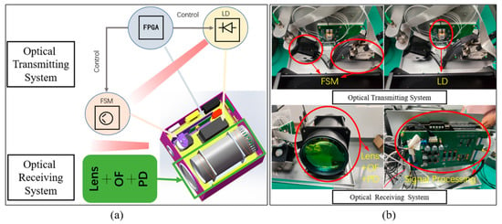
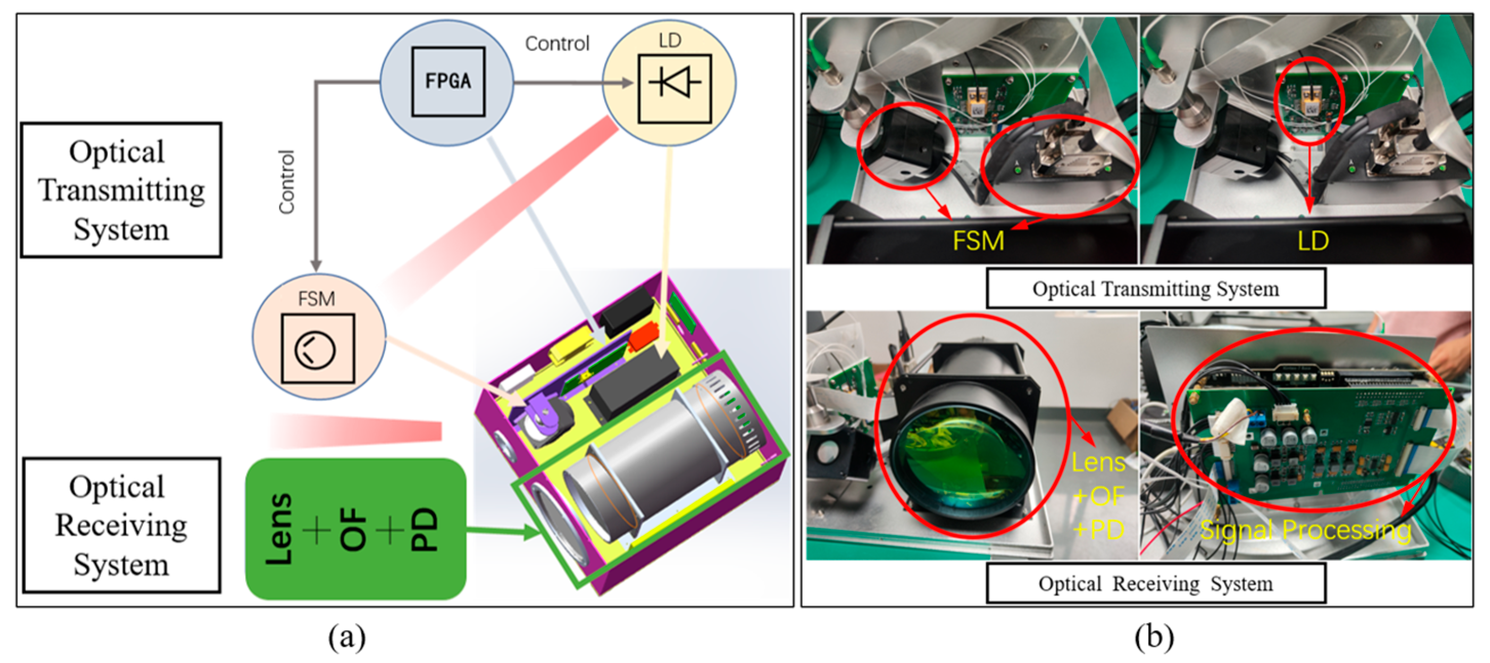
In the simulation, the influences of the number of scan points, noise near zero, and the step size of optical intensity values on curve fitting, as well as the effects of spot radius and scanning circle radius on tracking accuracy and communication quality, are analyzed. Based on this, the number of scan points N = 16 and the step size of optical intensity values m = 256 are selected to implement the algorithm computation process on FPGA, considering system performance and computational load. The integrated laser communication tracking and pointing prototype, as shown in Figure 11, is developed for on-ground static testing and link establishment testing to validate the alignment scheme and system.
Figure 11.
(a) The composition of the laser communication fine tracking prototype; (b) The physical diagram of the laser communication fine tracking prototype. (LD: Laser Diode; FPGA: Field-Programmable Gate Array; FSM: Fast Steering Mirror; OF: Optical Filter; PD: Photodetector).
The prototype mainly includes a transmitter and a receiver. The overall size is 30 cm × 40 cm × 40 cm, the weight is 15 kg, and the average power consumption is less than 30 W, which has relative size and power consumption advantages compared with the 60–80 W classical spaceborne laser communication terminals (SCOT80). The transmitter consists of LD, FPGA, and FSM. The receiver comprises receiving lens, OF, PD, and signal processing module, which are used to receive the optical signal and perform optical power information calculation. Before rotation locking and tracking, the two transceiver prototypes at opposite ends control their respective beams to carry out mutual rectangular spiral scanning to determine the approximate position range of the light spot.
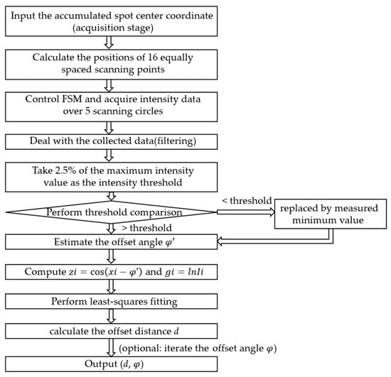
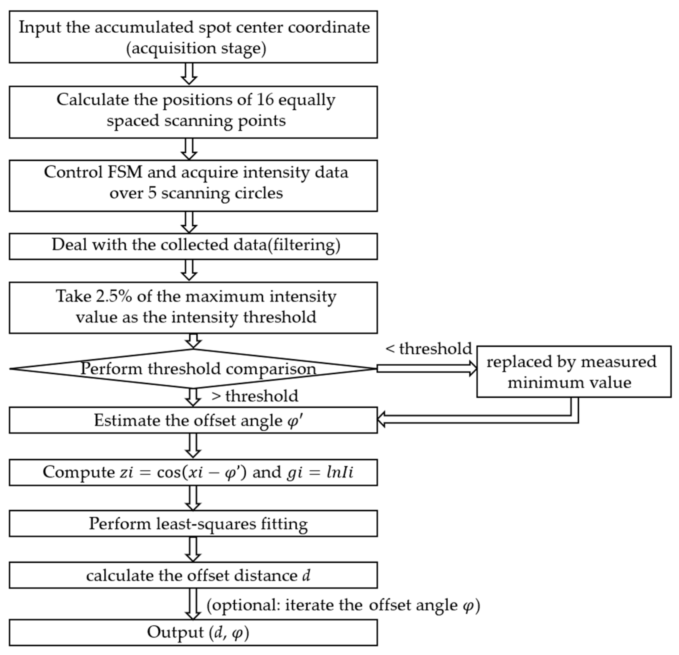
The specific fine-tracking fitting workflow is shown in Figure 12, and the steps are as follows: 1. obtain and input the coordinates of the accumulated spot center determined during the acquisition stage; 2. compute the coordinates of 16 equally spaced points on a circle of preset radius centered at the accumulated spot center; 3. control the fast steering mirror (FSM) to sequentially point to each scanning position and acquire optical intensity data at 5 complete circles, with each circle containing 16 points; 4. deal with optical intensity data by averaging and filtering; 5. take 2.5% of the maximum intensity value among all scanning points as the threshold and compare each data; 6. estimate an approximate offset angle using Equation (6) or (7) based on the scanning angles of the point with maximum intensity and its neighboring point; 7. perform a least squares fit on the set of points to obtain the parameters of the linear model and fit offset distance from Equation (13); 8. use Equation (8) to iteratively update, further reducing the angle estimation error if higher accuracy is required. The key parameters and their meanings in the algorithm can be found in Table 4.
Figure 12.
The algorithm flow chart of the rotation-locking alignment scheme.
Table 4.
The key parameters and their meanings in the algorithm.
The output results data will be written into the control frame of the communication data back to the transmitter and control the FSM to achieve alignment. Therefore, the prototype can achieve acquisition and pointing without a beacon optical system or common aperture for transmitting and receiving, and the overall equipment volume and weight are significantly reduced. Compared with traditional fine tracking systems [11,12,13], the prototype features simpler structure with lightweight and miniaturization for spaceborne laser communication applications.
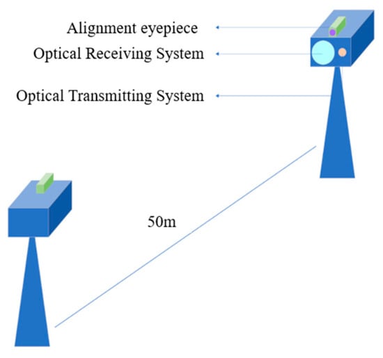
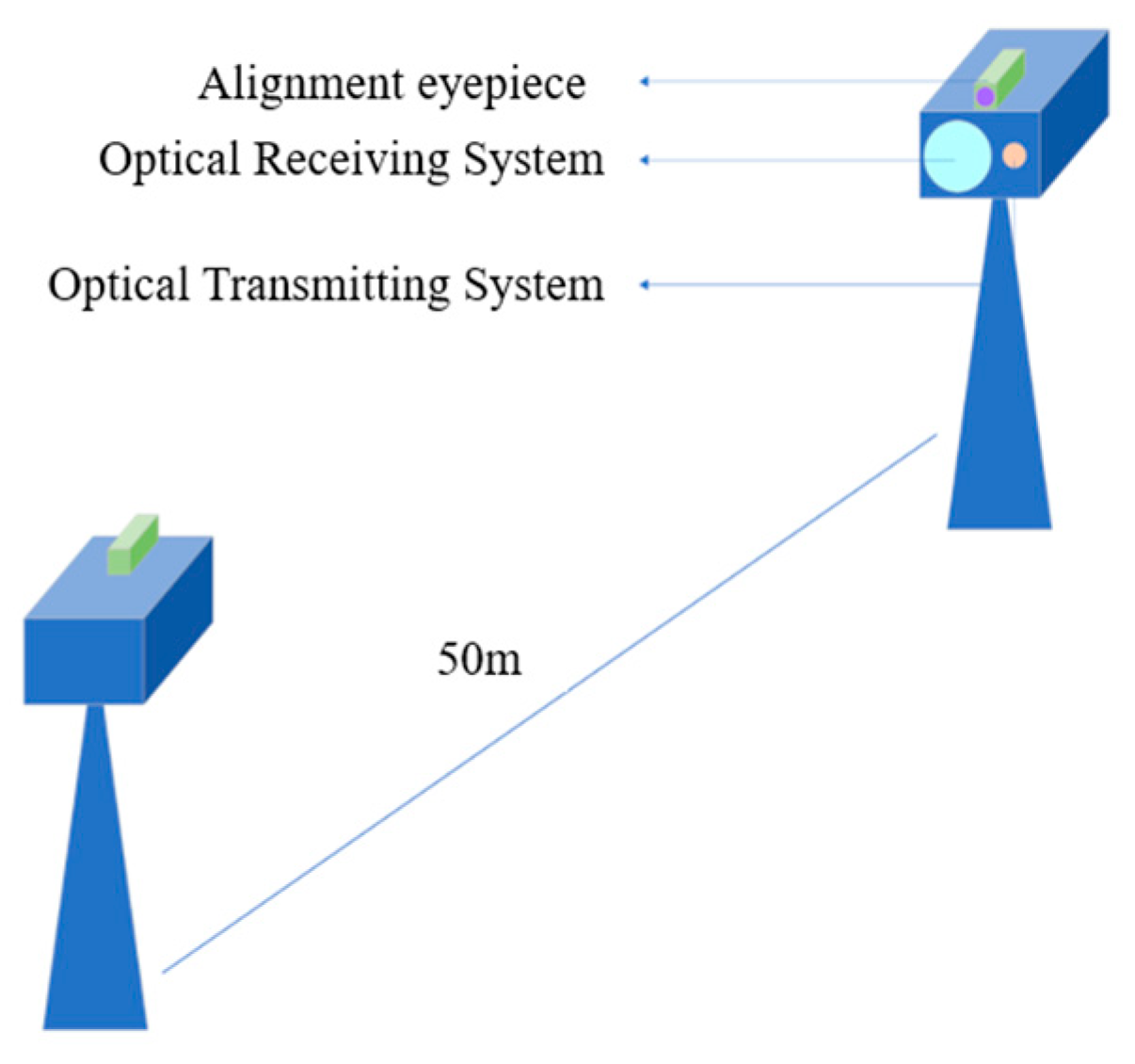
In the experiment, the rectangular spiral scanning method is used for coarse tracking to obtain cumulative spot position coordinates. After preliminary alignment, the transmitter controls the spot to perform rotational scanning. The static test setup is shown in Figure 13, where two transceiver prototypes as the transmitter and receiver are placed at opposite ends with 50 m transmission distance. The transmission system of the prototype consists of a laser and a collimator. To avoid self-transmission and self-reception, the signal optical wavelength at the two ends is 915 nm and 975 nm, respectively. The theoretical collimation angle of the collimator is approximately 3 mrad, and the system divergence angle is simulated about 4 mrad. The scanning circle radius is selected as 1 mrad considering both communication quality and tracking accuracy. Other useful system parameters are listed in Table 5. The system performs acquisition, tracking and communication in the same optical path without a beacon optical signal.
Figure 13.
The 50 m transmission distance static test diagram.
Table 5.
The prototype parameters in the experiment.
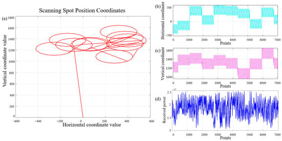
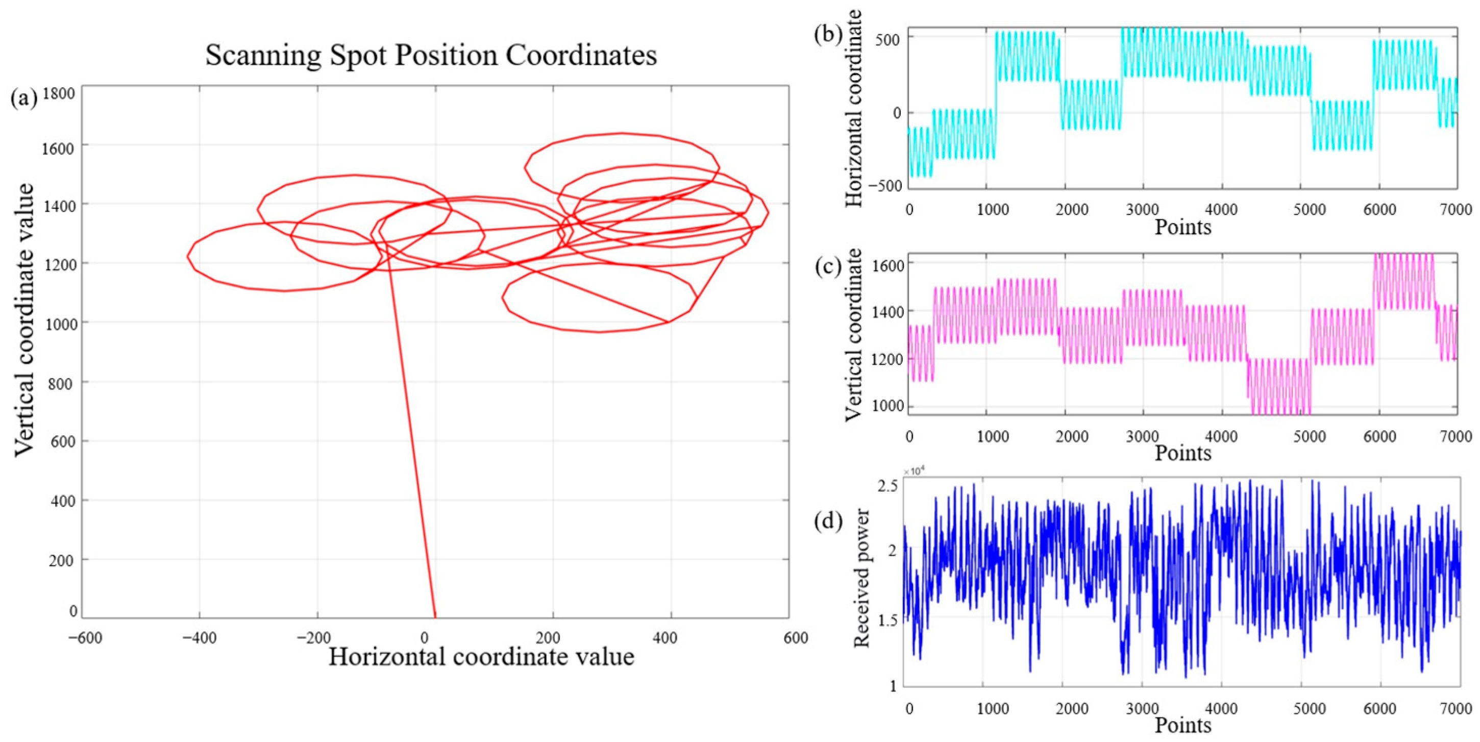
The scanning results are shown in Figure 14, where Figure 14a presents the positional coordinates of the scanning spot, while Figure 14b and Figure 14c, respectively, illustrate the variations in its horizontal and vertical coordinates. In addition, Figure 14d shows the optical intensity data collected five times by receiver at each scan point. The average value will be calculated by removing the maximum and minimum values to reduce intensity acquisition errors in the following data computation. The minimum threshold is set in the scanning process. When the received intensity falls below this threshold, it is automatically replaced with the minimum intensity value for calculation to prevent incidental factors from causing an excessively large calculated offset distance and leading to link interruption.
Figure 14.
Circular scanning results of the static test: (a) scanning spot position coordinates at multiple times; (b) horizontal axis variation at different scanning points; (c) vertical axis variation at different scanning points; (d) received optical power intensity at different scanning points.
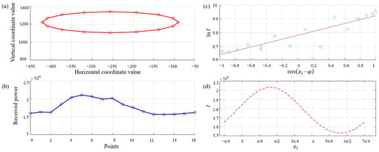
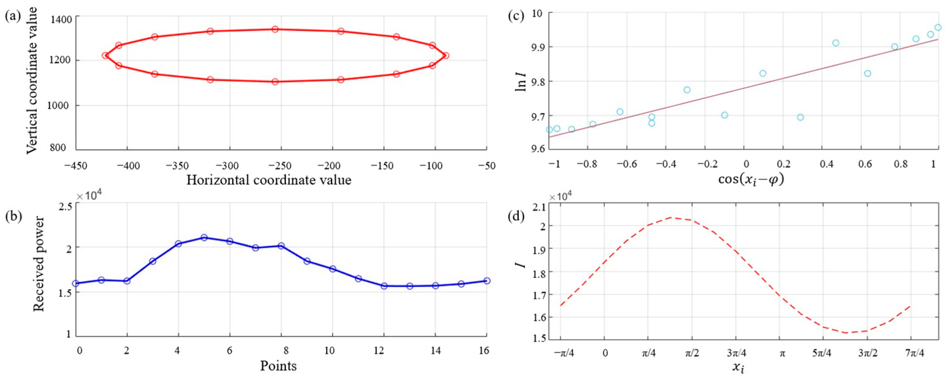
The single scan results, including positional coordinates and their optical intensity data, are used to fit the scanning curve and compute and d in Figure 15 with scan circle coordinates, intensity variation, regression line, and fitted scanning curve. Due to the complexity of calculating the arccosine function on FPGA, the is directly replaced by . The fitted offset at this moment is and d = 4 mm. From the system received lens focal length is 86 mm, the equivalent upper bound of residual pointing error is estimated to be approximately 0.465 mrad by the equation .
Figure 15.
Single scan results and fitted curve: (a) scanning points coordinates (red circles); (b) received optical power intensity at each scanning point (blue circles); (c) linear regression fitting curve of and (purple line); (d) fitting curve of scanning point angle xi and received optical power I (red dashed line).
After obtaining the receiver’s position (offset angle and offset distance), the calculated data will be written into the control frame of the optical communication data. The opposite terminal, which demodulates the control frame, will drive the FSM to adjust the optical path and achieve lock. Once the lock is established, the movement of the receiver is mainly related to slow-varying factors such as temperature changes in the spaceborne environment where no atmospheric turbulence exists. The received communication optical power can be used to judge the link alignment or misalignment. If the received optical power falls below the preset threshold, the system re-enters the fine-tracking process and performs rotation scanning again to maintain the locked state.
The fine-tracking system is an open-loop control structure with the locking process consisting only of scanning, fitting, and correction, just needing to iterate once or twice, and the convergence time mainly depends on the FSM’s control response time and the fitting computation time. Based on the system parameters in Table 5, the theoretical convergence time for single scan-correction cycle is estimated to be about 81.1 ms, consisting of three steps: 1. Rotational scanning: scanning 16 equally spaced points on the circular path, repeating for 5 circles, and taking at least 80 ms. 2. Fitting calculation: after obtaining the average optical intensity for each point, filtering and normalizing the data, and then fitting the offset distance and offset angle and taking < 0.1 ms under the 100 MHz main clock frequency. 3. Correction execution: generating the FSM driving voltage and the FSM responding approximately 1 ms, which corresponds to the theoretical equivalent tracking bandwidth of approximately 13 Hz.
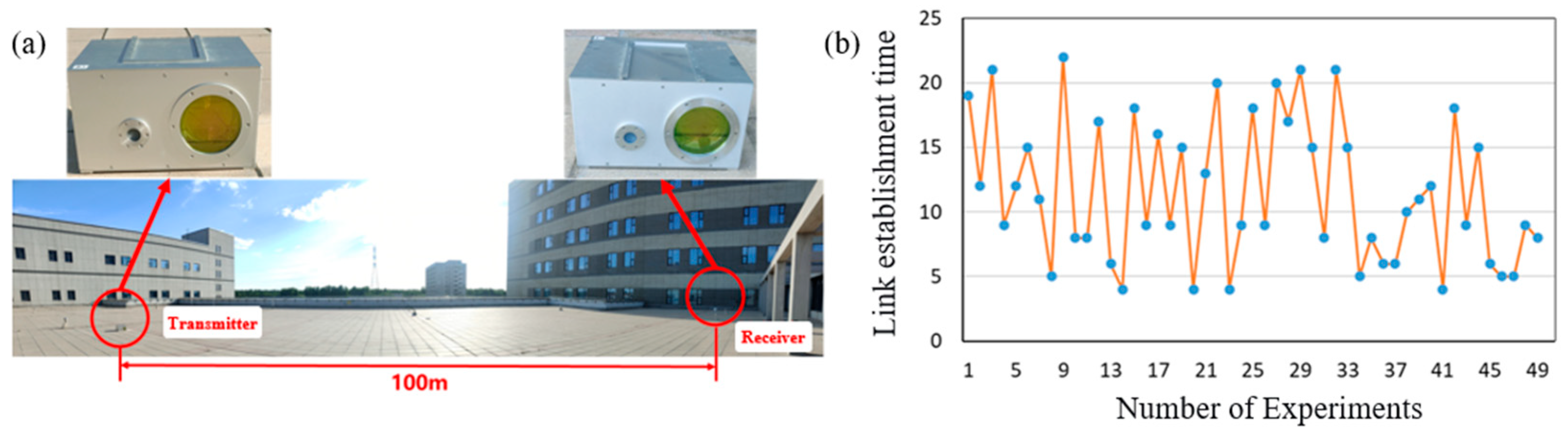
To verify the actual link establishment performance of the scheme, the link establishment test of the prototype is conducted in a 100 m outdoor environment, as shown in Figure 16. The ATP prototype adopts a rectangular spiral scanning method for the initial acquisition process, which performs a full coverage cyclic scan over the entire uncertainty region, and then enters the rotation locking stage to achieve a fine track. In the 100 m link establishment experiment, the receiving end is placed on a trolley and gently pushed to generate displacement changes at about 0.1 m/s to trigger the acquisition process to qualitatively validate the system’s re-acquisition capability against low-frequency displacement disturbances at the Hz level.
Figure 16.
Outdoor link establishment test setup and link establishment time: (a) outdoor experiment environment; (b) link establishment time at 49 times acquisition process, the blue points represent the measured link establishment time at each time and the orange line represents the trend of link establishment time.
The devices can successfully interlock with each other within 1 min after startup. When the communication link is briefly obstructed, the two devices can quickly re-establish the link. In 50 experiments, the system successfully acquired the link 49 times, yielding 98% acquisition probability. The shortest link establishment time, which measured the total time from the acquisition until the stable tracking, was 3 s, and the longest was 22 s. The average link establishment time was approximately 14.1 s. The standard deviation is 5.6 s and the 95% confidence interval is [12.5 s, 15.7 s], which is in the same performance range as the complete link acquisition time, about 22 s, of the XY-2 satellite. It demonstrates the scheme is capable of maintaining stable alignment for laser communication links. The main limiting factor of link establishment time is the scanning duration of initial acquisition, rather than the rotation-locking step. This indicates that the convergence speed of the rotation-locking process is much faster than that of the coarse acquisition stage. The link establishment time can be further reduced by optimizing the acquisition method.
A –61 dBm optical attenuator is artificially added at the transmitter side to simulate the link power budget of spaceborne long-distance applications. Although the 100 m terrestrial link distance is much shorter than intersatellite link, the optical power signal ultimately received by the system falls into an extremely weak-signal fitting regime, achieving –50 dBm detection sensitivity. Moreover, the atmospheric turbulence and background stray light interference introduced by the ground environment produce a signal-to-noise ratio (SNR) degradation that is, to some extent, equivalent to that of long-distance space transmission. In contrast, the spaceborne environment is free of atmospheric turbulence and features more ideal optical intensity distribution. Therefore, the success of the ground experiments demonstrates that the algorithm tolerates a certain level of optical intensity fluctuation, verifying its robustness. It indicates that the system has the potential to meet the power transmission attenuation requirements for future spaceborne long-distance applications.
5. Conclusions and Discussion
In summary, this paper proposes a fine tracking scheme and system that meets the miniaturization and lightweight requirements of spaceborne laser communication APT technology. By rotational spot scanning, the complex Gaussian spot intensity is transformed into a simple linear equation form, enabling the fitting calculation of the offset angle and offset distance between the receiver and the received spot center with effectively reduced computational complexity. The prototype is designed to conduct ground-based validation experiments to validate the algorithm, including laboratory static test and outdoor link establishment test. The experimental results demonstrate that the scheme can achieve stable tracking and link establishment.
Due to the lack of spaceborne validation conditions, the 50 link-break and re-establishment experiments during the 100 m outdoor link test, achieved by moving the receiver on a movable cart, demonstrates that the system can work stably under low-frequency jitter at the Hz level. But its ability to suppress high-frequency jitter is limited by the open-loop manner. Further research will be carried out quantitatively about the system performance of the next-generation prototype, including the convergence boundary tests from gradually increasing the initial offset to determine the capture range, the disturbance frequency sweep tests from 0.1 Hz to 30 Hz and measuring optical power fluctuation and re-acquisition success rate, and the additive noise injection and background light interference tests to determine the minimum operational SNR threshold.
And compared with the ground environment, where atmospheric turbulence exists, the spaceborne environment is free of turbulence effects and exhibits much weaker optical intensity scintillation, which is more ideal. However, the spaceborne environment involves other challenges, which are not considered in this paper, and future work will revolve around this aspect. Therefore, the scheme of rotation locking provides a possible approach for low-Earth-orbit (LEO) satellite laser communication terminals that have strict constraints on size and weight and where disturbances are dominated by low-frequency, slow temperature drifts. Further work will focus on vacuum compatibility design and the use of a satellite vibration table to load realistic on-orbit disturbance spectra, quantitatively determining the system’s dynamic response boundaries, so as to bridge the gap between ground experiments and actual orbital operating conditions.
Author Contributions
Conceptualization, J.W. and N.S.; methodology, J.W. and N.S.; software, J.W. and N.S.; validation, J.W., F.L. and N.S.; formal analysis, J.W. and N.S.; investigation, J.W.; data curation, J.W. and N.S.; writing—original draft preparation, J.W.; writing—review and editing, N.S. and H.Z.; supervision, H.Z.; project administration, J.L. All authors have read and agreed to the published version of the manuscript.
Funding
This research received no external funding.
Institutional Review Board Statement
Not applicable.
Informed Consent Statement
Not applicable.
Data Availability Statement
Data are contained within the article.
Conflicts of Interest
Author Ning Sun was employed by the company IEIT SYSTEMS Co., Ltd. Inspur. The remaining authors declare that the research was conducted in the absence of any commercial or financial relationships that could be construed as a potential conflict of interest. The funders had no role in the design of the study; in the collection, analyses, or interpretation of data; in the writing of the manuscript; or in the decision to publish the results.
References
- Chow, C.W. Optical Wireless Communication–Recent Progresses and Future Perspectives. J. Lightwave Technol. 2026, 44, 806–820. [Google Scholar] [CrossRef] [Scilit]
- Wadud, A.; Basalamah, A. Optical Wireless Communications for Next-Generation Radio Access Networks. ICT Express 2025, 11, 721–727. [Google Scholar] [CrossRef] [Scilit]
- Toyoshima, M. Recent Trends in Space Laser Communications for Small Satellites and Constellations. J. Lightwave Technol. 2021, 39, 693–699. [Google Scholar] [CrossRef] [Scilit]
- Ivanov, H.; Mejri, S.; Di Mira, A.; Schulz, K.; Heese, C. Review of Deep Space Optical Communications. Satell. Commun. Netw. 2025, 43, 193–209. [Google Scholar] [CrossRef] [Scilit]
- Toyoshima, M. Satellite Optical Communications for Beyond 5G/6G. In Proceedings of the 2025 IEEE Photonics Society Summer Topicals Meeting Series (SUM), Berlin, Germany, 21–23 July 2025; IEEE: Berlin, Germany, 2025; pp. 1–2. [Google Scholar]
- Wang, H.; Yao, K.; Gong, L.; Jin, Y.; Zhang, P.; Liu, Y.; Yuan, Y.; Xue, J.; Wan, Z.; Liu, Y.; et al. Space Computing Constellation: System Architecture, Implementations, and Challenges. IEEE Internet Things J. 2026, 13, 11472–11492. [Google Scholar] [CrossRef] [Scilit]
- Chen, W.; Sun, J.; Hou, X.; Zhu, R.; Hou, P.; Yang, Y.; Gao, M.; Lei, L.; Xie, K.; Huang, M.; et al. 5.12Gbps Optical Communication Link between LEO Satellite and Ground Station. In Proceedings of the 2017 IEEE International Conference on Space Optical Systems and Applications (ICSOS), Naha, Japan, 14–16 November 2017; IEEE: Naha, Japan, 2017; pp. 260–263. [Google Scholar]
- Cheng, M.-C.; Hsu, H.-Y.; Hayle, S.T.; Lu, H.-H.; Hsu, W.-W.; Okram, K.; Bai, Y.-Y.; Lu, J.-M.; Chung, Y.-C. A Simulated 1000-Km LEO Satellite-to-Ground Station Laser Communication Using a 1.8-Km OWC Link. J. Lightwave Technol. 2025, 43, 4731–4739. [Google Scholar] [CrossRef] [Scilit]
- Jet Propulsion Laboratory. 2023 Annual Report. Available online: https://d2pn8kiwq2w21t.cloudfront.net/documents/2023-annual-report.pdf (accessed on 24 May 2026).
- Ecale, E.; Torelli, F.; Tanco, I. JUICE Interplanetary Operations Design: Drivers and Challenges. In Proceedings of the 2018 SpaceOps Conference, Marseille, France, 28 May–1 June 2018; American Institute of Aeronautics and Astronautics: Marseille, France, 2018. [Google Scholar]
- Rose, T.S.; Rowen, D.W.; LaLumondiere, S.; Werner, N.I.; Linares, R.; Faler, A.; Wicker, J.; Coffman, C.M.; Maul, G.A.; Chien, D.H.; et al. Optical Communications Downlink from a 1.5U Cubesat: OCSD Program. In Proceedings of the International Conference on Space Optics—ICSO 2018, Chania, Greece, 9–12 October 2018; Karafolas, N., Sodnik, Z., Cugny, B., Eds.; SPIE: Chania, Greece, 2019; p. 18. [Google Scholar]
- Rose, T.S.; Rowen, D.W.; Coffman, C.M.; Kinum, G.; LaLumondiere, S.D.; Werner, N.I.; Wicker, J.M.; Maul, G.A.; Welle, R.P. Optical Downlink and Intersatellite Illumination Experiments with Low-Earth Orbiting CubeSats. In Proceedings of the Free-Space Laser Communications XXXII, San Francisco, CA, USA, 3–4 February 2020; Hemmati, H., Boroson, D.M., Eds.; SPIE: San Francisco, CA, USA, 2020; p. 61. [Google Scholar]
- Biswas, A.; Srinivasan, M.; Andrews, K.S.; Velasco, A.E.; Alerstam, E.; Allmaras, J.P.; Wollman, E.E.; Meenehan, S.M.; Wright, M.W.; Rogalin, R. Overview of the Deep Space Optical Communications (DSOC) Technology Demonstration. In Proceedings of the Free-Space Laser Communications XXXVII, San Francisco, CA, USA, 28–31 January 2025; Hemmati, H., Robinson, B.S., Eds.; SPIE: San Francisco, CA, USA, 2025; p. 21. [Google Scholar]
- Sodnik, Z.; Smit, H.; Sans, M.; Giggenbach, D.; Becker, P.; Mata-Calvo, R.; Fuchs, C.; Zayer, I.; Lanucara, M.; Schulz, K.-J.; et al. Results from a Lunar Laser Communication Experiment between NASA’s LADEE Satellite and ESA’s Optical Ground Station. In Proceedings of the SPIE International Conference on Space Optics—ICSO 2014, Tenerife, Spain, 7–10 October 2014; SPIE: San Francisco, CA, USA, 2014; Volume 10563, Article No. 1056309. [Google Scholar]
- Xue, W.; Liu, Y.; Zhu, X.; Wang, M.; Weng, Z.; Su, Y.; Yang, Y.; Zhao, H.; Wang, Y.; Chen, H.; et al. A High-Performance 10 Mm Diameter MEMS Fast Steering Mirror with Integrated Piezoresistive Angle Sensors for Laser Inter-Satellite Links. Microsyst. Nanoeng. 2025, 11, 75. [Google Scholar] [CrossRef] [Scilit] [PubMed]
- Abdelfatah, R.; Alshaer, N.; Ismail, T. A Review on Pointing, Acquisition, and Tracking Approaches in UAV-Based Fso Communication Systems. Opt. Quant. Electron. 2022, 54, 571. [Google Scholar] [CrossRef] [Scilit]
- Kaymak, Y.; Rojas-Cessa, R.; Feng, J.; Ansari, N.; Zhou, M.; Zhang, T. A Survey on Acquisition, Tracking, and Pointing Mechanisms for Mobile Free-Space Optical Communications. IEEE Commun. Surv. Tutor. 2018, 20, 1104–1123. [Google Scholar] [CrossRef] [Scilit]
- Chen, L.; Zhu, L.; Du, H.; Wang, X.; Shen, S.; Wang, Y.; Zhao, S.; Wang, X. Pointing Acquisition and Tracking System for Free Space Optical Communication Based on Integrated Optical Phased Array. IEEE Photonics J. 2025, 17, 7301608. [Google Scholar] [CrossRef] [Scilit]
- Li, Q.; Liu, L.; Ma, X.; Chen, S.-L.; Yun, H.; Tang, S. Development of Multitarget Acquisition, Pointing, and Tracking System for Airborne Laser Communication. IEEE Trans. Ind. Inf. 2019, 15, 1720–1729. [Google Scholar] [CrossRef] [Scilit]
- Lv, C.; Tong, S.; Song, Y. Optimization Design and Demonstration of Compound-Axis APT in Airborne Laser Communication. In Proceedings of the 2012 Symposium on Photonics and Optoelectronics, Shanghai, China, 21–23 May 2012; IEEE: Shanghai, China, 2012; pp. 1–4. [Google Scholar]
- Deng, D.; Xia, Z.; Wei, C.; Shao, J.; Fan, Z. Far-Field Intensity Distribution, M2 Factor of Beams Generated by Gaussian Mirror Resonator. Optik 2007, 118, 533–536. [Google Scholar] [CrossRef] [Scilit]
- Kochkina, E.; Wanner, G.; Schmelzer, D.; Tröbs, M.; Heinzel, G. Modeling of the General Astigmatic Gaussian Beam and Its Propagation through 3D Optical Systems. Appl. Opt. 2013, 52, 6030. [Google Scholar] [CrossRef] [Scilit] [PubMed]

Disclaimer/Publisher’s Note: The statements, opinions and data contained in all publications are solely those of the individual author(s) and contributor(s) and not of MDPI and/or the editor(s). MDPI and/or the editor(s) disclaim responsibility for any injury to people or property resulting from any ideas, methods, instructions or products referred to in the content. |
© 2026 by the authors. Licensee MDPI, Basel, Switzerland. This article is an open access article distributed under the terms and conditions of the Creative Commons Attribution (CC BY) license.