Adaptive Hartmann–Shack Wavefront Sensor

Abstract

In this work, an adaptive Hartmann–Shack wavefront sensor (AHSS) is proposed, designed, and evaluated. This sensor allows for the modification in the dynamic range of wavefront aberration measurement, defined as the range between the minimum and maximum aberration value that can be measured with the sensor. This capability makes it suitable for studying optical aberrations in both objective systems and the human eye. AHSS consists of sixteen phase profiles corresponding to microlens arrays designed to be projected (one at a time) onto a spatial light modulator (SLM). In each design, the microlens size and focal distance parameters were varied. A calibration process was conducted, and aberration measurements were made in both artificial and real eyes. The results demonstrate good correspondence between the measurements with the AHSS and a conventional Hartmann–Shack sensor, which uses an actual refractive microlens array with fixed size and focal length parameters, proving their feasibility for measuring optical aberrations. The AHSS opens up possibilities for measurements in eyes with special characteristics, such as high aberrations, and enables the implementation of active optics aberration correction systems without the need for an additional refractive (physically lensed) wavefront sensor.

1. Introduction

The conventional refractive Hartmann–Shack sensor (HSS) comprises a two-dimensional array of microlenses with identical characteristics, including focal length and diameter. The microlens array detects local wavefront slopes by sampling the wavefront through each microlens, projecting a set of luminous spots onto a camera. For a wavefront without aberrations, the microlenses generate spots that form a regular grid at the focal plane, establishing a reference for measuring aberrated wavefronts. By comparing the reference position of the spots to the displacements caused by an aberrated wavefront, the local average slopes of the wavefront are quantified. This straightforward method for wavefront measurement makes the HSS a preferred sensor in visual simulators. However, it has limitations due to its fixed sensitivity and dynamic range [1], determined by the microlenses’ size (p) and focal length (f), restricting its ability to measure a wide range of optical aberrations. Consequently, this presents a slight disadvantage when measuring aberrations from more complex optical systems.

While ideas have been explored to extend the dynamic range of the HSS, often relying on more efficient computational algorithms for centroid determination [2,3], by simultaneously implementing multiple arrays of microlenses [4,5,6], micro-mirrors [7], the use of artificial intelligence [8,9,10], and dynamic optical elements such as spatial light modulators (SLMs) and electro-optic lenses (EOLs) [11,12,13,14,15,16], the SLMs and EOLs provide the opportunity to create adaptive versions of the HSS. Due to their ease of acting on the wavefront and their relatively fast processing, these elements enable adjustable configurations where the sensitivity and dynamic range of the HSS can be tailored to the optical system being evaluated. However, as far as we know, their applicability in real eyes has not yet been studied. Therefore, this work proposes and evaluates adaptive Hartmann–Shack sensors that can modify their dynamic range to study optical aberrations in both objective systems (such as an artificial eye) and the human eye, thereby overcoming the limitations of the conventional HSS.

2. Materials and Methods

For the experimental implementation of the adaptive sensor, a phase-only SLM (pixel size of 8 μm, PLUTO NIR-011, Holoeye Photonics AG, Berlin, Germany) was used to project the phase of microlens arrays. These arrays were generated as phase maps of spherical lenses arranged in a homogeneous matrix pattern (1920 × 1080 pixels), which were programmed and projected onto the SLM. Four values of microlens sizes pitch, (p) = 0.864, 0.648, 0.540, and 0.432 mm, were evaluated, each with four values of focal length f = 30, 50, 70, and 100 mm. This resulted in sixteen different phases of microlens arrays being tested.

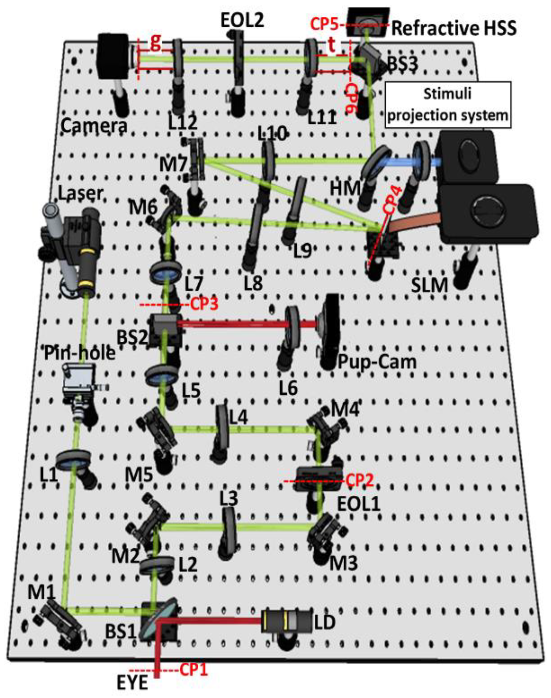
The SLM was integrated into a monocular visual simulator equipped with active optics, as shown in Figure 1. This simulator operates based on the optical conjugation of different planes within the optical system using afocal systems composed of achromatic doublets. In these planes, elements such as an eye (artificial or real), an EOL ($EOL1$, model EL-16-40-TC-VIS-20D, Optotune, Bernstrasse, Switzerland), an SLM, and a refractive HSS (CMOS camera with a resolution of 1024 × 1280 pixels and 0.200 mm microlens size (pitch) with a 7 mm focal length; Flexible OKO Optical, Rijswijk, The Netherlands) are located [17]. In this simulator, a pellicle beam splitter (BS3) was positioned between the hot mirror (HM) and the refractive HSS in the setup, allowing for simultaneous aberration measurements by the AHSS and the refractive HSS. The complete optical setup is depicted in Figure 1.

The methodology to perform a wavefront measurement with the AHSS involves projecting the phase pattern selected from the designed set of microlenses onto the SLM so the light from the optical element being tested generates a pattern of points at the focal distance of the microlenses. Subsequently, an afocal system was constructed using achromatic lenses $L11$ and $L12$ with equal focal lengths of 10 cm to obtain images on the sensor plane of a monochromatic CMOS camera (model acA2000-165um, Basler ace, Ahrensburg, Germany). Additionally, an EOL, ($EOL2$, model EL-10-30-TC-VIS-12D, Optotune, Bernstrasse, Switzerland) was placed in the focal plane of lens $L11$. This EOL allows for adjustment of the relay system’s optical power by varying the current applied to it. In this way, the focal spot patterns generated by the phases of the microlenses projected onto the SLM can be imaged on the CMOS camera, which is conveniently placed at a distance g from $L12$ [18]. The objective was to use $L11, L12$ and $EOL2$ to refocus this pattern of points onto the camera. Since the AHSS has varying focal lengths, this refocusing process must be carried out for each individual microlenses focal length design. This setup is similar to the one proposed by Martínez-Cuenca et al. (2010) [11], which enables an easily refocusable process through the EOL.

The advantage of this configuration, with $EOL2$ in the focal plane of $L11$, is that the magnification between the conjugate planes of the system and the camera does not change when $EOL2$’s optical power is modified. Thus, the separation of focal spots on the camera remains constant regardless of the focal length of the microlenses projected on the SLM. According to the work of Martínez-Cuenca et al. (2010) [11], it is possible to establish a relationship between the optical power programmed in the $EOL2$ and the focal length of the designed microlenses projected onto the SLM for achieving proper focus on the camera. This relationship is given by:

$$P_{EOL2}={\displaystyle \frac{f_{L11}-t}{f_{L11}^2}}+{\displaystyle \frac{f_{L12}-\mathsf{g}}{f_{L12}^2}}+{\displaystyle \frac{f_{CP}}{f_{L11}^2}},$$

(1)

where $P_{EOL2}$ is the optical power of the $EOL2$; $f_{L11}$ and $f_{L12}$ are the focal lengths of $L11$ and $L12$, respectively; $f_{CP}$ is the focal length of the microlenses projected onto the SLM but rescaled on the sensor plane of the camera; and $t$ and g are the distances from $CP6$ to $L11$, and from $L12$ to the camera, respectively (see Figure 1). With this expression, it is possible to determine the optical power that should be programmed into the $EOL2$ to maintain well-focused the spots pattern on the camera without changing the magnification.

As evident from Equation (1), the optical power of the $EOL2$ depends on the designed focal length of the microlenses projected onto the SLM but rescaled to the conjugate plane due to the magnification of the system (0.6✕). To determine the appropriate optical powers for $EOL2$ based on these re-scaled focal lengths, the parameters t and g in Equation (1) were computationally varied to find optical-power values that were within the programmable range of the $EOL2$ employed in this setup. It was found that the optimal values corresponded to t = 5 cm and g = 5 cm, respectively. These values allowed us to determine the variation range of the optical power $P_{EOL2}$ as a function of $f_{CP}$. Finally, to achieve precise values of the optical power $P_{EOL2}$, it was necessary to know the relationship between the electrical current applied to the $EOL2$ and its variation in optical power. This relationship was established in the work developed and published by Torres-Sepúlveda et al. [18].

2.1. AHSS Calibration

The calibration involved generating known spherical wavefronts (defocus only) and measuring them with the AHSS to study the relationship between the optical power measured with the AHSS and the power induced on the system by $EOL1$. This setup allows for the induction of the desired vergence (defocus) on the light by varying the electric current used to control $EOL1$.

Additionally, the variation in astigmatism and the Root Mean Square (RMS) of high-order aberrations was studied as a function of the induced defocus. The objective was to determine which parameters of the designed profiles of the microlenses of the AHSS best fit hypothetical measurements of any optical system, aiming for calibration curves similar to those obtained with the refractive HSS, which was taken as the reference wavefront sensor for comparison. The calibration of the AHSS was conducted for a wavelength of 532 nm, and the corresponding AHSS microlenses phases were designed and projected onto the SLM using this same wavelength. The AHSS spots images corresponding to the microlens size of 0.864 mm were processed only up to the 4th order (14 Zernike terms) since there were not enough microlenses to efficiently sample the wavefront within a pupil size of 4.8 mm [19]. The remaining AHSS spots images were processed up to the 5th order (21 Zernike terms), similar to the refractive HSS.

2.2. Measurements of Optical Aberrations in an Artificial Eye

As a first test, the performance of the AHSS was evaluated for measuring the optical aberrations of an artificial eye. This artificial eye consisted of an achromatic lens and a rotating diffuser screen that served as a retina. This screen was displaced an arbitrary distance from the lens to simulate an eye with a degree of hyperopia. The aberration measurements on the artificial eye were carried out using a diode laser with a wavelength of 780 nm (model L780P010, 10 mW, Ø5.6 mm, Thorlabs Inc., Newton, NJ, USA), necessitating a redesign of the microlens phase patterns projected on the SLM to this wavelength. The optical aberrations of this artificial eye were measured using the sixteen microlens phases designed for the AHSS and compared to those measured with the refractive HSS. For each AHSS microlens phase, aberrations were measured three times, with $EOL1$ at a defocus of 0 Diopters (D) (i.e., only the intrinsic aberrations of the artificial eye were measured). The measurements from the sixteen AHSS microlenses phases were subsequently compared to the measurements obtained with the refractive HSS.

2.3. Measurements of Optical Aberrations in a Real Eye

The measurements of optical aberrations in real eyes were conducted using eight of the AHSS microlens phases, selected based on the results from measurements in the artificial eye. These phases corresponded to the four values of pitch (p) with focal distances of 30 and 50 mm, as they produced higher-quality spot patterns in the presence of speckle compared to other microlens phases. Optical aberration measurements were performed on three subjects using the eight AHSS microlens phases and the refractive HSS. The subjects were aged between 26 and 41 years and had healthy eyes with no history of ocular surgery. The exclusion criteria included patients with astigmatism greater than 0.5 D. The eyes’ subjective refraction was corrected using $EOL1$, with their refraction ranging from [−0.5 to 0.5] D. Astigmatism and high-order aberrations were not corrected. Accommodation was paralyzed with two drops of 1% tropicamide ophthalmic solution. Informed consent was obtained from the patients after explaining the nature and possible consequences of this study. This study was approved by the Bioethics Committee of the University Research Center (Sede de Investigación Universitaria) from the University of Antioquia, Medellín, Colombia. The measurement protocols adhered to the tenets of the Declaration of Helsinki [20].

Aberrations were measured on each subject using both the refractive HSS and the AHSS for a 4.8 mm processing pupil (pupil size measured in the conjugate plane of the subject’s eye; see Figure 1). In general, all HSS images obtained from real eyes contain speckle noise. To partially reduce this effect, average images obtained from a video of approximately four seconds (around 70 frames) were processed, which reduced the influence of speckle. In all cases, the average images had better quality than an individual video frame and, therefore, could be correctly processed with the wavefront sensor software, without presenting high variability in the results. Based on these measurements, the aberrations obtained from the refractive HSS and the AHSS were compared to determine the latter’s capability for measuring ocular aberrations. Measurements were performed on the dominant eye of each subject (sighting dominance as determined using the Miles criterion [21]). All custom-made routines to process the videos and images were developed in Matlab 2021a (Matlab; Mathworks, Natick, MA, USA).

3. Results

3.1. AHSS Calibration

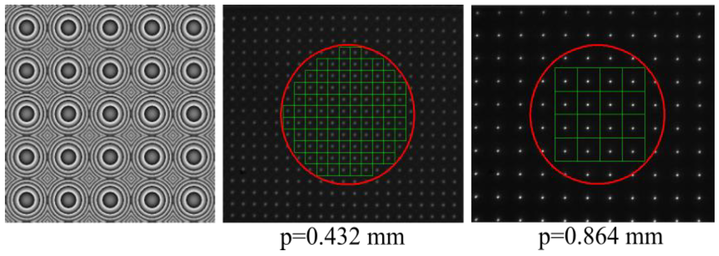
Figure 2 shows an example of the phase map of a microlens array projected on the SLM and examples of the images captured with the camera by different configurations of microlenses used in the adaptive sensor. These images exhibit the high quality of the obtained spot maps, indicating accurate modulation of light by the SLM. They illustrate two of the four evaluated microlens sizes. For pitch (p) = 0.864 mm, it can be observed that there are few spots within the evaluated area (red circles in Figure 2, denoting a diameter size of 4.8 mm on the pupil plane of the eye). For this particular case, only Zernike polynomials up to the 4th degree are considered.

Because the main advantage of the proposed AHSS is the possibility of modifying its dynamic range and sensitivity, both parameters were estimated for the sixteen implemented microlens phase-map configurations. The estimation was performed using the geometrical relationship reported in [19]:

$$tan \theta ={\displaystyle \frac{d}{2f}},$$

(2)

where $\theta$ represents the local wavefront slope, d is the displacement interval considered on the detector, and f is the focal length of the microlens phase map. To estimate the dynamic range, d was taken as the microlens pitch (p), which defines the maximum allowable spot displacement before ambiguity between adjacent microlens regions occurs. To estimate the sensitivity, d was taken as the CMOS camera pixel size, 5.5 μm, which represents the minimum detectable spot displacement considered in this approximation. Because the microlens phase maps are re-imaged through the relay system, the values reported in

Table 1. Estimated dynamic range and sensitivity values for the sixteen AHSS configurations implemented with different microlens pitch (p) and focal length (f) parameters. The values were calculated using the geometrical relationship described in Equation (2).

AHSS	Dynamic Range $\mathbf{(}\mathit{r}\mathit{a}\mathit{d}\mathbf{)}\mathbf{\times }{10}^{\mathbf{-}3}$	Sensitivity $\mathbf{(}\mathit{r}\mathit{a}\mathit{d}\mathbf{)}\mathbf{\times }{10}^{\mathbf{-}3}$
p = 0.432 mm; f = 30 mm	12.1	0.026
p = 0.540 mm; f = 30 mm	15.1	0.026
p = 0.648 mm; f = 30 mm	18.1	0.026
p = 0.864 mm; f = 30 mm	24.1	0.026
p = 0.432 mm; f = 50 mm	7.2	0.015
p = 0.540 mm; f = 50 mm	9.0	0.015
p = 0.648 mm; f = 50 mm	10.8	0.015
p = 0.864 mm; f = 50 mm	14.4	0.015
p = 0.432 mm; f = 70 mm	5.2	0.011
p = 0.540 mm; f = 70 mm	6.4	0.011
p = 0.648 mm; f = 70 mm	7.7	0.011
p = 0.864 mm; f = 70 mm	10.3	0.011
p = 0.432 mm; f = 100 mm	3.6	0.008
p = 0.540 mm; f = 100 mm	4.5	0.008
p = 0.648 mm; f = 100 mm	5.4	0.008
p = 0.864 mm; f = 100 mm	7.2	0.008
HSS p = 0.2 mm; f = 7 mm	14.3	0.039

were calculated using the effective pitch and focal length at the corresponding conjugate plane. The resulting values, summarized in Table 1, show the expected trade-off between dynamic range and sensitivity: increasing the microlens pitch increases the measurable angular range, whereas increasing the focal length improves angular sensitivity.

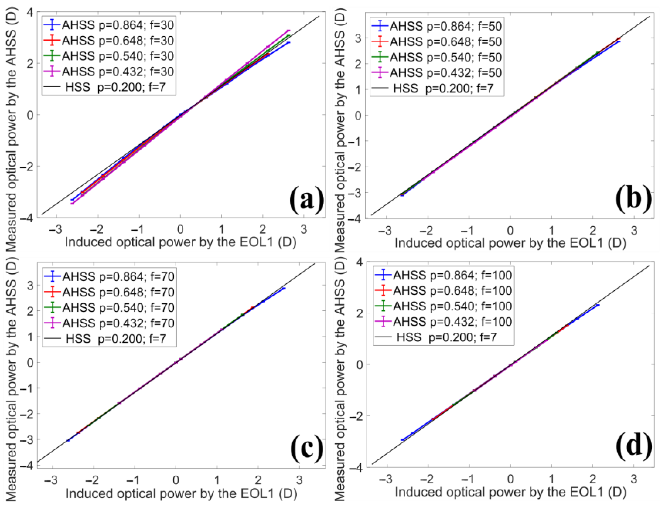
Figure 3 illustrates the optical power calibration curves. Each plot represents the measured optical power as a function of the induced optical power for the sixteen proposed microlenses phase maps of the AHSS and the refractive HSS. As expected, a linear relationship was obtained between optical powers in all cases. All AHSS configurations exhibit calibration slopes similar to those obtained with the refractive HSS. The effective focal length of each microlens array, used by the AHSS to calculate aberrations, is determined by multiplying the designed focal length by the slope of each calibration curve.

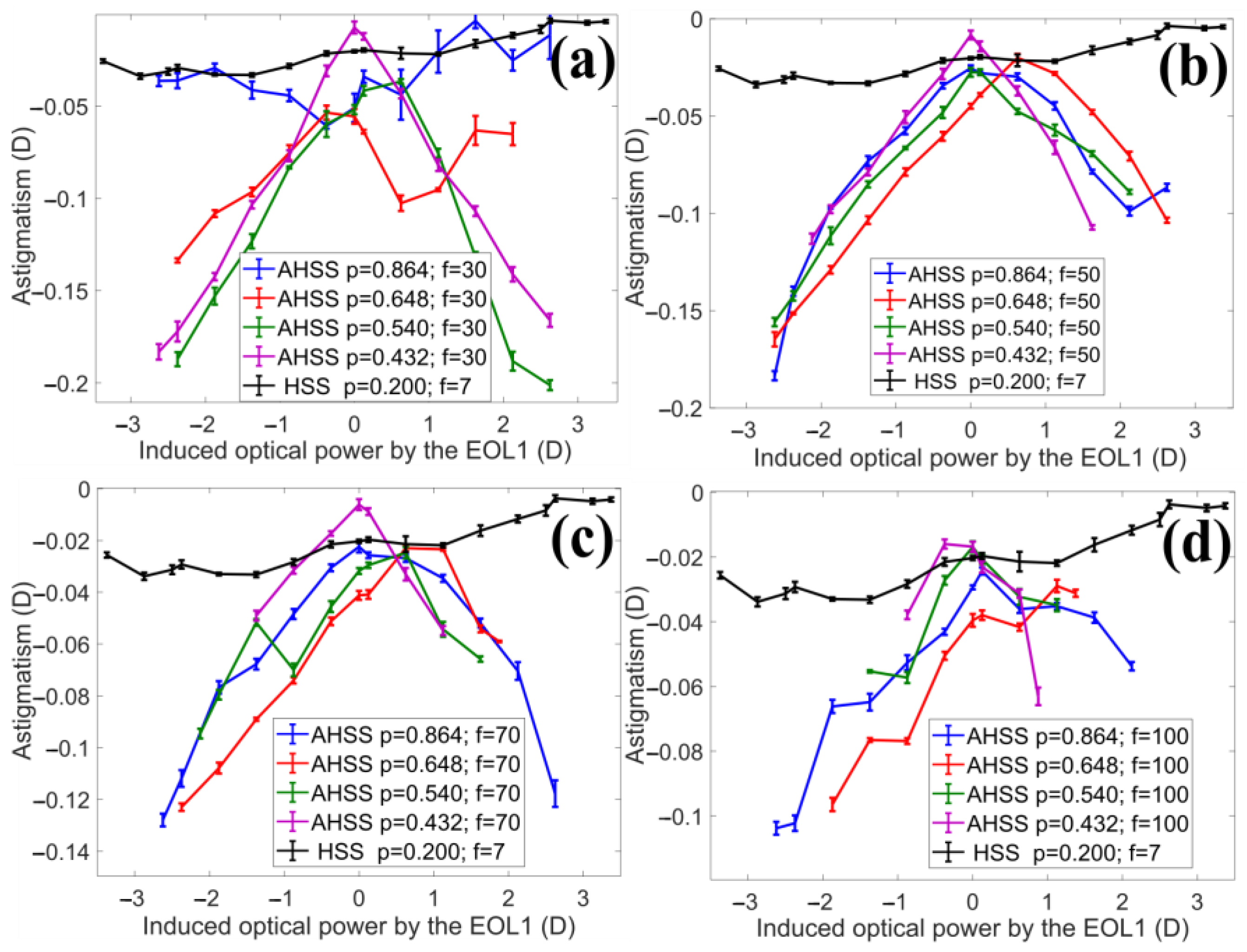
On the other hand, Figure 4 shows the behavior of astigmatism as a function of induced optical power for each phase map of the AHSS and the refractive HSS. In this figure, an increase in astigmatism measured with the AHSS compared to that measured by the refractive HSS (black line) is observed, with values reaching less than 1/5 diopter. These values should be considered when obtaining isolated measurements from artificial or real eyes, as they represent system-specific aberrations (reference). As observed, the measured astigmatism is greater when using microlens phase maps with smaller focal lengths, which may be attributed to the arrangement of different optical elements used in the experimental system (this will be explored in the Discussion section). The refractive HSS, on the other hand, exhibits nearly constant behavior, ranging between −0.05 and 0 D of induced astigmatism. In all cases, the values do not represent significant effects on visual quality in the human eye, as shown in the study by Leube et al. [22].

The calibration results in Figure 3 and Figure 4 are expressed in diopters (D) because the induced defocus was defined as a variation in refractive power. In the following sections, however, aberrations are reported in micrometers (μm), corresponding to the reconstructed Zernike wavefront coefficients. For comparison purposes, the Zernike defocus coefficient can be converted into an equivalent refractive defocus using the relationship described by Nam et al. [23]:

$$D={\displaystyle \frac{-4\sqrt{3}}{r^2}} C_2^0,$$

(3)

where $D$ is the equivalent defocus in diopters, r is the pupil radius in millimeters, and $C_2^0$ is the Zernike defocus coefficient in micrometers.

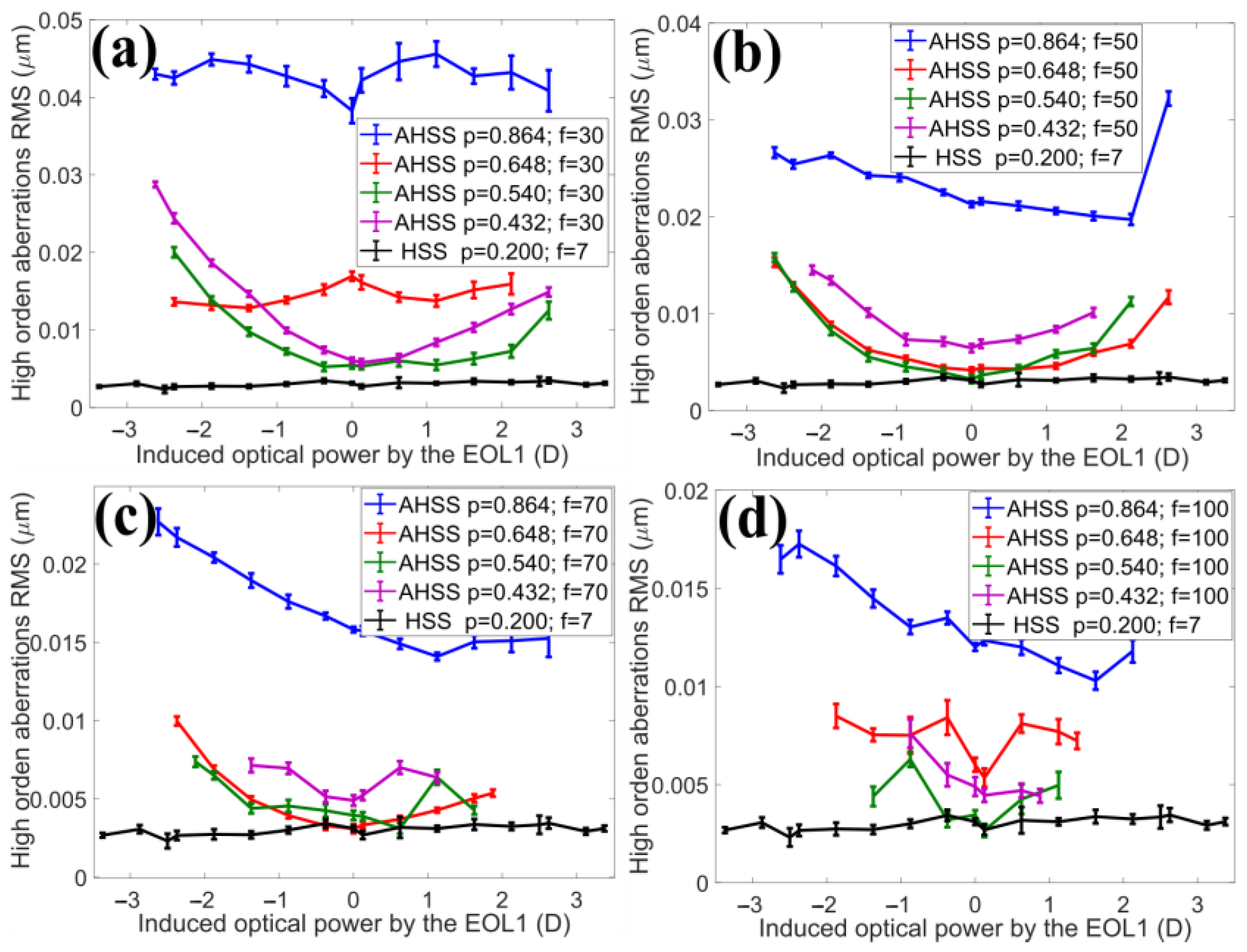
Figure 5 illustrates the variation in the RMS of high-order aberrations when different values of optical power are induced in the system, showing an increase in the RMS value measured with the AHSS compared to the refractive HSS case. This nearly one-order-of-magnitude increase in RMS is small but should be considered when evaluating optical aberrations of an isolated system. Consistent with the behavior of the astigmatism, these values were higher for AHSS microlens arrays designed with shorter focal lengths. On the other hand, an important effect to highlight is that regardless of the focal length, the case of pitch (p) = 0.864 mm (AHSS with the largest microlens size) consistently generated the highest RMS. This may be attributed to it being the case with the lowest number of Zernike terms (4th degree, 14 terms) for aberration measurement, increasing the error in determining the exact values of the Zernike coefficients representing the wavefront. Despite this limitation, in general, the calibration results demonstrated a good correspondence between the refractive HSS and the AHSS. Additionally, they showed that the key characteristics of the AHSS, such as dynamic range and sensitivity, could be easily controlled and adjusted by varying the AHSS phase profiles projected onto the SLM.

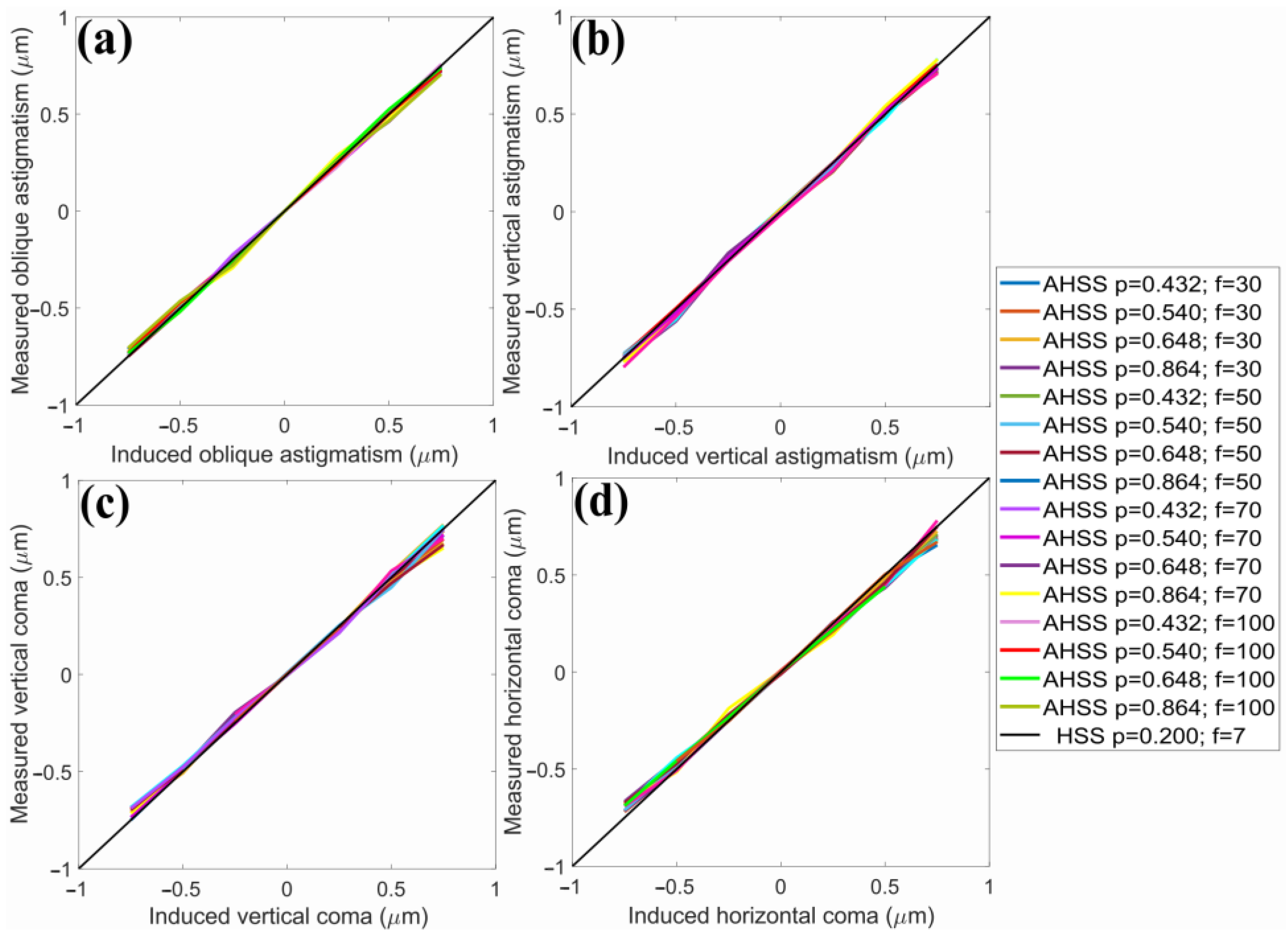
To further evaluate the AHSS response to aberration modes other than defocus, additional calibration experiments were performed for astigmatism and coma. These aberrations were induced using an auxiliary SLM placed at the eye’s pupil plane (CP1, see Figure 1). This auxiliary SLM, identical to that described previously (PLUTO NIR-011, Holoeye Photonics AG, Berlin, Germany), was used to generate individual Zernike modes, whereas the AHSS SLM projected the microlens phase maps corresponding to the sixteen sensor configurations. This experimental arrangement allowed the response of each AHSS phase map to know astigmatism and coma terms to be evaluated. Figure 6 shows the relationship between the induced aberrations and the corresponding measurements obtained with the sixteen AHSS configurations and the refractive HSS. In all cases, a predominantly linear response, with slopes close to unity, was observed. These results indicate that the proposed AHSS provides consistent measurements not only for defocus but also for astigmatism and higher-order aberration terms such as coma.

3.2. Measurements of Optical Aberrations in an Artificial Eye

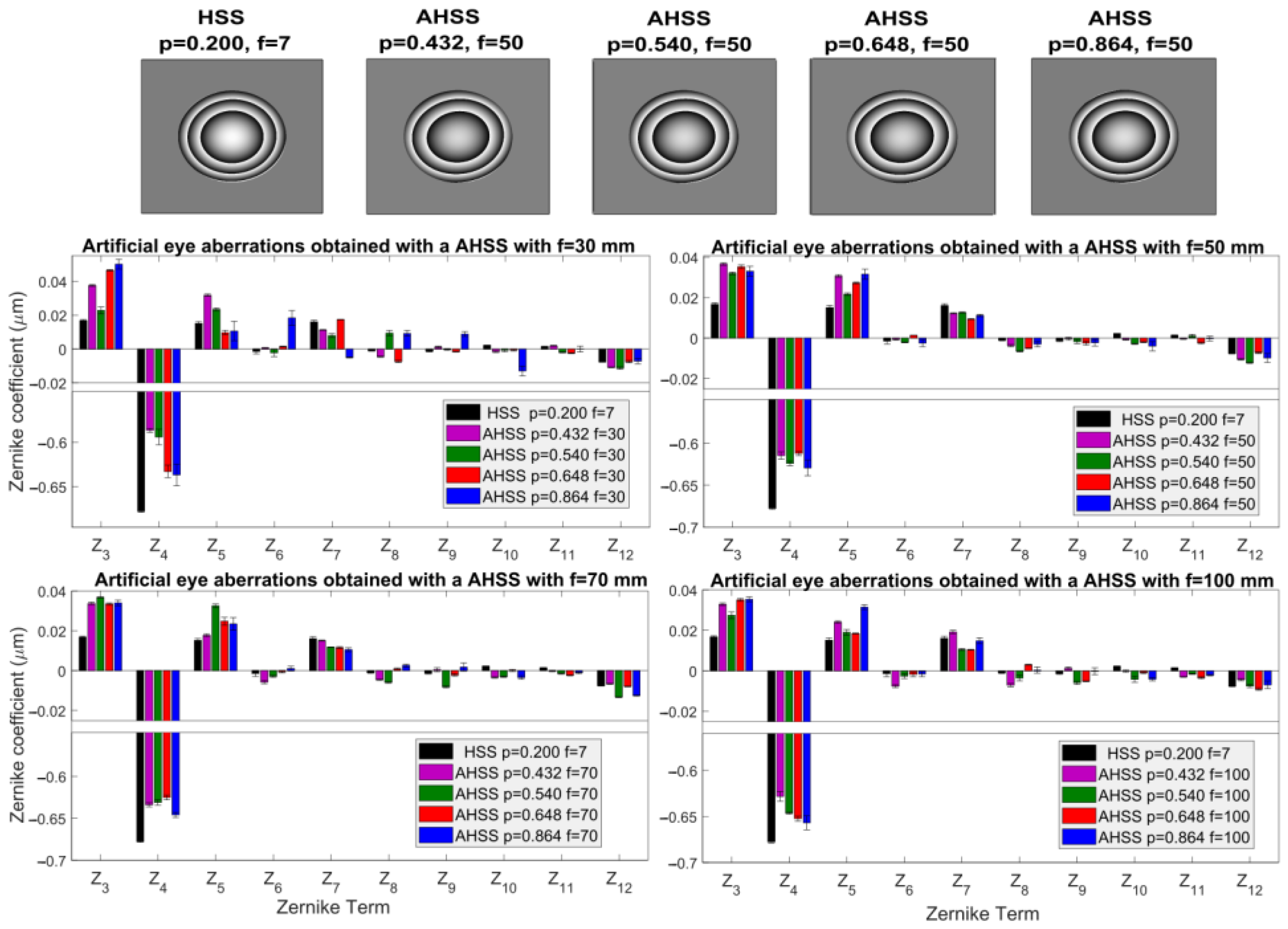
The aberration measurements were conducted using a plane wavefront as a reference to eliminate system-specific aberrations measured with the AHSS or the refractive HSS. The reference images are taken from the calibration process detailed in the previous section. Thus, the measured aberrations correspond solely to those of the artificial eye (excluding the intrinsic aberrations of the system). The top of Figure 7 provides an example of the wavefront maps obtained with the AHSS. These wavefront maps were constructed by averaging the Zernike coefficients measured three times with the AHSS and were compared with the assumed gold-standard case of the refractive HSS. It is observed that defocus predominates, consistent with the refractive error induced in the artificial eye. The plots of Figure 7, on the other hand, represent a comprehensive comparison of measurements taken with the AHSS for each focal length value (30, 50, 70, and 100 mm) for the four designed microlens sizes and the refractive HSS (as mentioned earlier, microlenses with pitch (p) = 0.864 mm have fewer Zernike terms evaluated).

Across all different microlens sizes, the Zernike terms demonstrate proper correspondence for identical focal lengths and exhibit minimal variance across varying focal lengths. Additionally, when comparing the results of the designed AHSS with the refractive HSS, it can be noted that for the defocus and astigmatism terms ($Z_4$, $Z_3$, and $Z_5$, corresponding to $Z_2^0$, $Z_2^{-2}$ and $Z_2^2$ in OSA notation, respectively), there are slight differences between the sensors. In contrast, the higher-order terms show sufficiently good agreement in both magnitude and sign. For pitch (p) = 0.864 mm, there are no significant differences despite the reduction in the number of Zernike terms in the processing, except for the case of focal length (f) = 30 mm, where discrepancies were observed compared to the other sensors, especially with respect to the refractive HSS (see Table S1 of the Supplementary Materials).

The small differences between sensors, especially in the measurements of high-order aberrations, indicate a good sensitivity of the AHSS, demonstrating its ability to accurately reproduce the measurement of small optical aberrations. Among the high-order aberrations, vertical coma and spherical aberration ($Z_7$ and $Z_{12}$, corresponding to $Z_3^{-1}$, $Z_4^0$ in OSA notation, respectively) are particularly noteworthy. A notable correspondence was found in these terms among all studied microlens phase maps of the AHSS. The other high-order aberration terms resulted in very small values, with differences that, from a visual optics standpoint, do not present significant effects.

3.3. Measurements of Optical Aberrations in Real Eyes

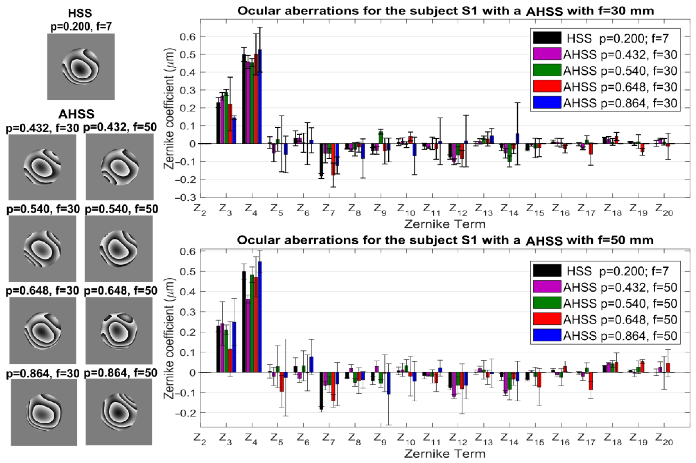
Figure 8 illustrates the phase maps and Zernike coefficients corresponding to the average of the three measurements taken with each microlens phase map of the AHSS for one of the three subjects measured in this study (subject S1). It can be observed that the phase maps with focal length (f) = 30 mm and f = 50 mm are comparable. Likewise, while the average values of the Zernike coefficients show apparent differences, the analysis of the error bars indicates that there are no statistically significant differences between the measurements with the AHSS and the refractive HSS (see Table S2 of the Supplementary Materials). Despite the variability among each sensor for the second-order coefficients, there were no statistically significant differences in those terms (defocus and astigmatism). Small differences were observed in high-order aberrations, with greater variability found for the microlens phase maps with pitch (p) = 0.864 mm for both focal length (f) = 30 mm and f = 50 mm.

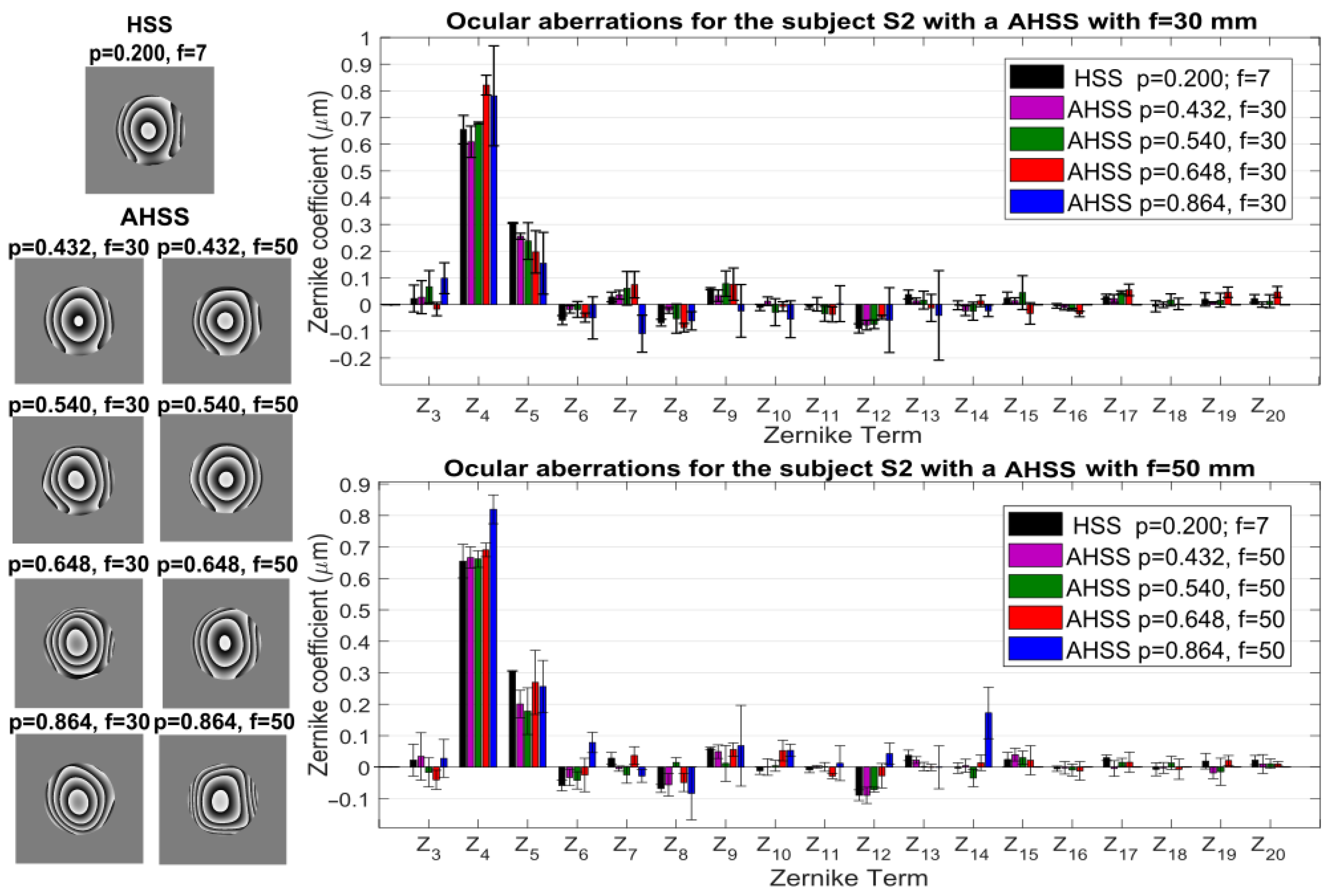
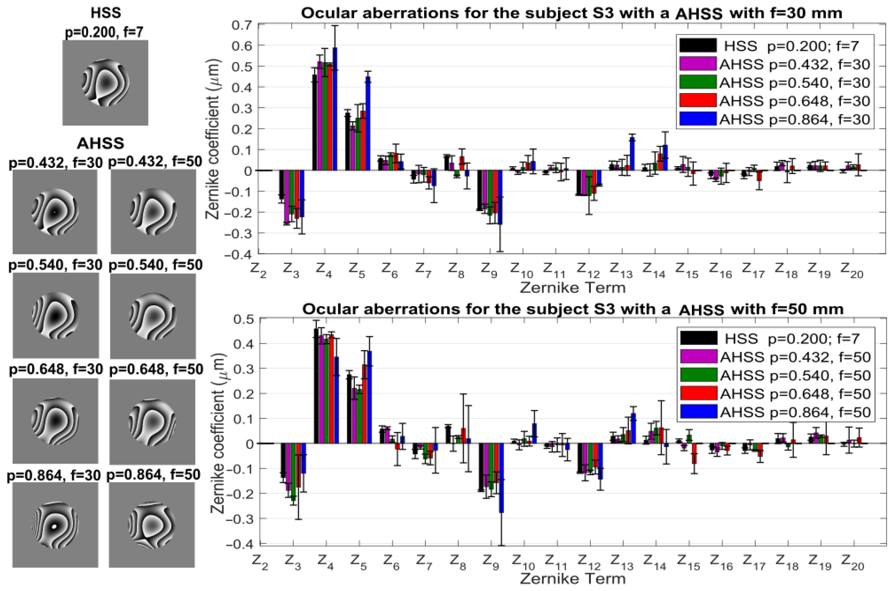
Similarly, Figure 9 displays the wavefront phase maps and Zernike coefficients obtained for subject S2. The figure highlights the similarity in the results obtained by all microlens phase maps of the AHSS and the refractive HSS. Additionally, no considerable differences were observed between the microlens phase maps with the two focal distances. Finally, Figure 10 shows the wavefront phase maps and Zernike coefficients obtained for subject S3. As with the previous subjects, the Zernike coefficient values coincide for all microlens phase maps of the AHSS. However, there is a noticeable discrepancy between the Zernike coefficients (and the respective maps) in the measurements obtained with the AHSS with the largest microlens size. This finding is consistent across the subjects. The high variability observed with the AHSS with the larger microlens size can be attributed to the limited number of terms in the expansion of Zernike polynomials.

The results obtained with real eyes confirm the capabilities of the AHSS for applications to more complex optical systems than the artificial eye. However, it was found that not all designed microlens phase maps of the AHSS are suitable for proper application in real eyes. First, a key aspect for measurements with a microlens phase map is related to the quality of each focal spot. The focal spots must be of sufficient quality to allow for the correct application of the specific algorithm that determines the centroid of the focal spot and, consequently, the precise calculation of its local displacement. This is fundamental, as it determines the local wavefront slope, and therefore, the correct reconstruction of the wavefront.

In this context, it was found that only the microlens phase maps of the AHSS with focal lengths of f = 30 mm and f = 50 mm provided focal spot arrays with sufficient quality for the correct application of the centroid calculation when used in real eyes. In contrast, the microlens phase maps with longer focal lengths produced images in which the focal spots could not be clearly distinguished. Additionally, considerable variation in the Zernike values (for the same subject) was observed in each measurement with large focal lengths, resulting in high variability in the results. This effect is due to the inherent limitation of the SLM’s spatial resolution for the projection of phase maps with large focal lengths and small apertures, which restricts wavefront sampling. For this reason, it was decided to use the microlens phase maps with shorter focal lengths, which exhibit better quality in the focal spot patterns and consequently, lower variability in the measurements.

4. Discussion

This work demonstrates the performance and functionality of the AHSS, which have reconfigurable parameters for measuring optical aberrations in static and more complex dynamic systems. In the implementation of the AHSS, the calibration process shows the behavior of the optical power, astigmatism, and high-order aberrations measured with the different microlens phase maps of the AHSS and in the refractive HSS as a function of the defocus generated by the $EOL1$. Good correspondence is found between the calibration results of the AHSS and the refractive HSS. These results illustrate how each microlens phase map parameter affects the measurements of the optical quality of the system, which is crucial when implementing them to study external optical systems.

The variations in the astigmatism curves shown in Figure 4 could be explained by the arrangement of the lenses in the monocular visual simulator with active optics [17]. When projecting the microlens array onto the SLM, a vergence of the light is generated depending on the corresponding focal length design, influenced by the location of the lenses in the visual simulator. For example, for the microlenses with f = 30 mm, the light focuses 3 cm from the Pluto-SLM plane, but, on its path, it encounters the first lens of the setup at 22 cm (see Figure 1; $L9$ lens). This implies that the light reaches the lens with a divergent wavefront, not fulfilling the paraxial approximation condition, because it passes through the entire area of the lens and not only the central. This effect makes the small remaining misalignments in the system more noticeable, thus causing an increase in the measured astigmatism of the system. Astigmatism values exceeding 0.25 diopters become noticeable in subjective visual assessments; however, the astigmatism detected by the AHSS, which is at most 0.2 D above the values measured by the refractive HSS, remains below this perceptual threshold. Consequently, the astigmatism values obtained within this optical system are sufficiently moderate to ensure accurate refraction measurements of a real eye without significant perceptual impact [22].

Additionally, the high-order RMS value was analyzed. It was calculated from the Zernike coefficients ranging from term $Z_6$ to $Z_{20}$ (corresponding to $Z_3^{-3}$, $Z_5^5$ in OSA notation, respectively), corresponding to the third to fifth order (Figure 5). Although differences were observed compared to the case of the refractive HSS, it is important to highlight that these RMS values are small compared to the typical RMS of a real human eye [24]. Therefore, they are not expected to have a significant impact on optical or visual quality in real ophthalmic applications. Despite the results showing consistency for all microlens phase maps with different focal lengths, an increase in the RMS value was observed for the microlenses associated with pitch (p) = 0.864 mm. This increase is attributed to the error introduced in the wavefront reconstruction, arising from using a reduced number of sampling points [19].

It is important to highlight that in the measurement methodology, the inherent aberrations of the system measured during the calibration process with the AHSS at each EOL power were taken as a reference. These reference measurements were then subtracted from the measurements obtained when evaluating additional optical systems, such as the artificial eye or a real eye. This compensation helps to control some of the differences in the aberration terms when compared with the refractive HSS. The results obtained in the calibration of the AHSS demonstrate that, in this initial study of reconfigurable AHSS, it is possible to achieve feasible measurements of real optical systems with easy control of their characteristics.

Additionally, the calibration experiments performed for astigmatism and coma aberrations showed a predominantly linear response for all AHSS configurations, indicating that the proposed sensor preserves consistent aberration measurements not only for defocus but also for higher-order aberration modes.

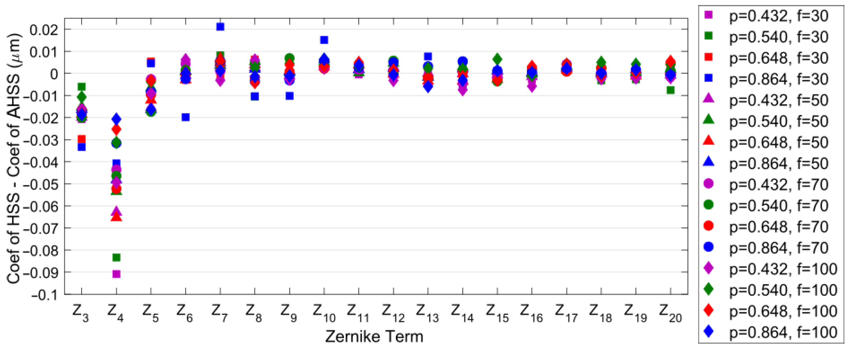
In this context, the differences between the coefficients measured by the refractive HSS and the sixteen microlens phase maps of the AHSS were calculated to quantify the variations in aberration measurements of the artificial eye. Figure 11 graphically shows these differences for each aberration coefficient and for each microlens phase map used.

It is important to emphasize that the greatest differences were found for the defocus coefficient ($Z_4$, corresponding to $Z_2^0$ in OSA notation), with an approximate value of −0.09 µm (around −0.11 diopters), corresponding to the microlens phase map defined by pitch (p) = 0.432 mm and a focal length (f) = 30 mm. The next notable difference was obtained for the oblique astigmatism coefficient ($Z_3$ corresponding to $Z_2^{-2}$ in OSA notation), with a maximum value of 0.03 µm, in the microlens phase map defined by pitch (p) = 0.864 mm and focal length (f) = 30 mm. For the rest of the high-order aberration coefficients, the differences were found in a range of [−0.01, 0.01] µm, except for the microlens phase map with pitch (p) = 0.864 mm and focal length (f) = 30 mm, where differences of up to 0.02 µm were present, which are still considerably small. These results demonstrate good agreement between the optical aberration measurements for static systems, such as the artificial eye, obtained with the AHSS and the conventional refractive HSS.

For a general evaluation of the differences between the AHSS and the refractive HSS in measuring the artificial eye’s aberrations, the RMS value of the differences between all the Zernike coefficients obtained with the refractive HSS and the different microlens phase maps of the AHSS was calculated. The calculation revealed that the differences were in the range of [0.007, 0.021] µm, where the minimum value corresponded to the microlens with pitch (p) = 0.648 mm and focal length (f) = 100 mm, and the maximum value to the microlens with pitch (p) = 0.432 mm and focal length (f) = 30 mm. Objectively, it is possible to determine that the differences are very small between the different microlens phase maps, indicating that all of them are potentially viable for performing aberration measurements in static optical systems, as well as in applications that require variations in the dynamic range of the sensors used.

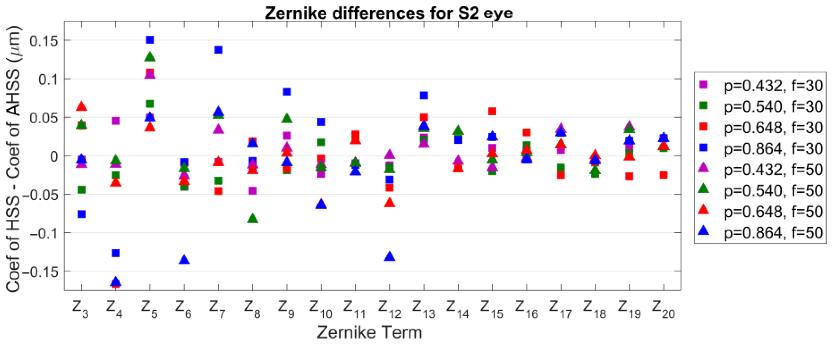
Similarly, to objectively determine the quality of the optical aberrations measurements obtained for real eyes, differences were calculated between the Zernike coefficients obtained with the refractive HSS and those obtained with the AHSS. Figure 12 shows the results of these differences for each Zernike coefficient for subject S2 (the results for subjects S1 and S3 are similar, as shown in Figure S1 of the Supplementary Materials). From Figure 12, it is notable that larger differences occur for coefficients associated with second-order Zernike polynomials, where maximum differences of ±0.16 µm were found (around 0.19 diopters in defocus and 0.31 diopters in astigmatism). These values fall within the range of typical variability observed in real eyes for defocus and astigmatism, as reported by Leube et al. [22]. While there are some exceptions, it can be noted that for high-order aberrations, most differences fall within the range of ±0.05 µm. This indicates good agreement with the results found previously for the artificial eye.

To objectively determine the subject-wise differences, the RMS value of the differences between the Zernike coefficients obtained with the refractive HSS and those obtained with each microlens phase map of the AHSS sensor was calculated.

Table 2. RMS of the differences between the Zernike coefficients of the refractive HSS and each microlens phase map of the AHSS. Values calculated for a pupil size of 4.8 mm at the eye’s pupil plane.

AHSS	S1	S2	S3
(p; f) mm	RMS (µm)	RMS (µm)	RMS (µm)
(0.432; 30)	0.035	0.023	0.036
(0.540; 30)	0.045	0.026	0.034
(0.648; 30)	0.024	0.051	0.031
(0.864; 30)	0.046	0.063	0.071
(0.432; 50)	0.052	0.028	0.027
(0.540; 50)	0.033	0.041	0.032
(0.648; 50)	0.045	0.030	0.034
(0.864; 50)	0.040	0.072	0.049

displays the RMS values of differences for each subject with each microlens. According to the values reported in Table 2, it is evident that the highest RMS value of differences occurs for the microlenses with pitch (p) = 0.864 mm, which is consistent with the results obtained previously in calibration and measurements on the artificial eye. For the remaining microlens phase maps, considerably small RMS of differences were observed for all subjects.

The presented results open a wide range of possibilities for implementing the proposed adaptive Hartmann–Shack sensors. For example, as a first implementation, the AHSS can be used as a preliminary mechanism allowing for partial measurement and later correction of optical aberrations in an active (open loop) or adaptive (close loop) optics system. The objective of this partial correction is to generate a wavefront with sufficient quality to be subsequently measured by a conventional refractive HSS sensor, which can perform a finer measurement and, therefore, provide a more precise correction. In other words, this procedure could extend the dynamic range of experimental systems and, consequently, open up possibilities for measurements in eyes with special characteristics, such as those with a high degree of myopia or more complex pathologies of refractive surfaces of the eye.

In addition, the use of the SLM in conjunction with the EOL and its rapid temporal response can facilitate the implementation of an open-loop aberration correction system. In this system, temporal multiplexing would be employed to measure and correct aberrations simultaneously, taking advantage of integration time. Similar modulation-based approaches have also been reported for reducing retinal speckle in live-eye wavefront sensing measurements [25]. This approach eliminates the need for a refractive HSS sensor, and the dynamic range of the AHSS sensor can be adjusted according to the specific eye being evaluated.

Future work will focus on experimentally evaluating the AHSS in dynamic measurement conditions, where changes in the aberration level or in the optical system under evaluation may require real-time selection of the microlens pitch and focal length to optimize the trade-off between sensitivity and dynamic range.

It is important to mention that, while the refractive HSS was used as a reference to compare the measurements and functionality of the AHSS, an AHSS with characteristics similar to the refractive one, i.e., with the same focal length and microlens size, was not constructed. Reproducing an AHSS with parameters identical to those of the refractive HSS is currently complex given the existing system design, mainly due to the spatial resolution limitations of the SLM. However, it is possible to modify this version to achieve a direct correspondence with the refractive sensor without further reducing the size of the microlens phase maps projected onto the modulator or decreasing the corresponding focal length. This can be done by choosing different focal lengths for the lenses that make up the relays in the experimental system. This way, a magnification between the conjugate optical planes less than 1✕ can be obtained, allowing both the size of the microlenses and the focal length to be rescaled. Thus, focal lengths similar to the refractive sensor’s 7 mm could be achieved. With this modification, it would be possible to make a direct comparison between an AHSS and a refractive HSS with identical characteristics, which is proposed as a future perspective of this work.

5. Conclusions

The adaptive Hartmann–Shack wavefront sensors designed, implemented, and evaluated in this study provided aberration measurements comparable to those obtained with a conventional refractive Hartmann–Shack sensor despite having considerably different parameters. This finding opens up possibilities for various applications of the reconfigurable AHSS tailored to the study of ocular optics, addressing the current demand for versatile and powerful methods for wavefront metrology and optical aberration characterization. A key advantage of the AHSS is its ability to modify its dynamic range, making it applicable to the study of optical aberrations in both objective optical systems (like an artificial eye) and the human eye. The AHSS enables measurements in eyes with special characteristics, such as a high degree of myopia or more complex pathologies of the refractive surfaces, by enabling adjustment of their dynamic range. Furthermore, the use of the SLM in conjunction with an EOL and its rapid temporal response can facilitate the implementation of an open-loop aberration correction system without the need for an additional refractive Hartmann–Shack sensor. In summary, the proposed and evaluated AHSS demonstrated good performance and functionality comparable to conventional refractive sensors, with the additional advantage of having reconfigurable parameters to adapt to different optical systems and applications in ocular optics.

References

1. Akondi, V.; Dubra, A. Shack-Hartmann wavefront sensor optical dynamic range. Opt. Express 2021, 29, 8417–8429. [Google Scholar] [CrossRef]
2. Xia, M.; Li, C.; Hu, L.; Cao, Z.; Mu, Q.; Xuan, L. Shack-Hartmann wavefront sensor with large dynamic range. J. Biomed. Opt. 2010, 15, 026009. [Google Scholar] [CrossRef]
3. Shinto, H.; Saita, Y.; Nomura, T. Shack-Hartmann wavefront sensor with large dynamic range by adaptive spot search method. Appl. Opt. 2016, 55, 5413–5418. [Google Scholar] [CrossRef]
4. Lindlein, N.; Pfund, J. Experimental results for expanding the dynamic range of a Shack-Hartmann sensor by using astigmatic microlenses. Opt. Eng. 2002, 41, 529–533. [Google Scholar] [CrossRef]
5. Shinto, H.; Saita, Y.; Nomura, T. Expansion of dynamic range in Shack-Hartmann wavefront sensor using dual microlens array. Biophotonics Jpn. 2015, 9792, 106–109. [Google Scholar]
6. Ares, M.; Royo, S.; Caum, J. Shack-Hartmann sensor based on a cylindrical microlens array. Opt. Lett. 2007, 32, 769–771. [Google Scholar] [CrossRef]
7. Vohnsen, B.; Martins, A.C.; Qaysi, S.; Sharmin, N. Hartmann shack wavefront sensing without a lenslet array using a digital micromirror device. Appl. Opt. 2018, 57, E199–E204. [Google Scholar] [CrossRef]
8. Hu, L.; Hu, S.; Gong, W.; Si, K. Deep learning assisted Shack-Hartmann wavefront sensor for direct wavefront detection. Opt. Lett. 2020, 45, 3741–3744. [Google Scholar] [CrossRef] [PubMed]
9. Yang, W.; Wang, J.; Wang, B. A Method Used to Improve the Dynamic Range of Shack-Hartmann Wavefront Sensor in Presence of Large Aberration. Sensors 2022, 22, 7120. [Google Scholar] [CrossRef] [PubMed]
10. Zhang, M.; Guo, Y. Performance Characterization of Deep-Phase-Retrieval Shack-Hartmann Wavefront Sensors. IEEE Photonics J. 2023, 15, 6801311. [Google Scholar] [CrossRef]
11. Martínez-Cuenca, R.; Durán, V.; Climent, V.; Tajahuerce, E.; Bará, S.; Ares, J.; Arines, J.; Martínez-Corral, M.; Lancis, J. Reconfigurable Shack–Hartmann sensor without moving elements. Opt. Lett. 2010, 35, 3. [Google Scholar] [CrossRef]
12. Saita, Y.; Shinto, H.; Nomura, T. Holographic Shack-Hartmann wavefront sensor based on the correlation peak displacement detection method for wavefront sensing with large dynamic range. Optica 2015, 2, 411–415. [Google Scholar] [CrossRef]
13. Aftab, M.; Choi, H.; Liang, R.; Kim, D.W. Adaptive Shack-Hartmann wavefront sensor accommodating large wavefront variations. Opt. Express 2018, 26, 34428–34441. [Google Scholar] [CrossRef]
14. Lechner, D.; Zepp, A.; Eichhorn, M.; Gladysz, S. Adaptable Shack-Hartmann wavefront sensor with diffractive lenslet arrays to mitigate the effects of scintillation. Opt. Express 2020, 28, 36188–36205. [Google Scholar] [CrossRef] [PubMed]
15. Pathak, B. An improved programmable grating array based wavefront sensor. Appl. Opt. Metrol. 2021, 11817, 161–168. [Google Scholar]
16. Akondi, V.; Castillo, S.; Vohnsen, B. Multi-faceted digital pyramid wavefront sensor. Opt. Commun. 2014, 323, 77–86. [Google Scholar] [CrossRef]
17. Torres-Sepúlveda, W.; Mira-Agudelo, A.; Barrera-Ramírez, J.F.; Petelczyc, K.; Kolodziejczyk, A. Optimization of the Light Sword Lens for Presbyopia Correction. Transl. Vis. Sci. Technol. 2020, 9, 6. [Google Scholar] [CrossRef] [PubMed]
18. Torres-Sepúlveda, W.; Henao, J.; Morales-Marín, J.; Mira-Agudelo, A.; Rueda, E. Hysteresis characterization of an electrically focus-tunable lens. Opt. Eng. 2020, 59, 044103. [Google Scholar] [CrossRef]
19. Porter, J.; Queener, H.M.; Lin, J.E.; Thorn, K.; Awwal, A.; Wiley, A.J. Adaptive Optics for Vision Science: Principles, Practices, Design and Applications; Wiley Interscience: Boston, MA, USA, 2006. [Google Scholar]
20. World Medical Association. World Medical Association Declaration of Helsinki: Ethical Principles for Medical Research Involving Human Subjects. JAMA 2013, 310, 2191–2194. [Google Scholar] [CrossRef]
21. Miles, W.R. Ocular dominance demonstrated by unconscious sighting. J. Exp. Psychol. 1929, 12, 113–126. [Google Scholar] [CrossRef]
22. Leube, A.; Leibig, C.; Ohlendorf, A.; Wahl, S. Machine Learning based Predictions of Subjective Refractive Errors of the Human Eye. In Proceedings of the 12th International Joint Conference on Biomedical Engineering Systems and Technologies, Prague, Czech Republic, 22–24 February 2019; pp. 199–205. [Google Scholar]
23. Nam, J.; Thibos, L.N.; Iskander, D.R. Zernike radial slope polynomials for wavefront reconstruction and refraction. J. Opt. Soc. Am. A 2009, 26, 1035–1048. [Google Scholar] [CrossRef] [PubMed]
24. Plainis, S.; Pallikaris, I. Ocular monochromatic aberration statistics in a large emmetropic population. J. Mod. Opt. 2008, 55, 759–772. [Google Scholar] [CrossRef]
25. Albanis, V.; Ribak, E.N.; Carmon, Y. Reduction of speckles in retinal reflection. Appl. Phys. Lett. 2007, 91, 054104. [Google Scholar] [CrossRef]
Figure 1. Experimental setup: Laser (532 nm wavelength); Pin-hole; L: lens; M: mirror; Camera: camera for imaging the AHSS spots patterns; BS: beam splitter; LD: laser diode; Pup-Cam: pupil camera; SLM: spatial light modulator; HM: hot mirror; CP: conjugate pupil plane (CP1 corresponds to the eye’s pupil plane); HSS: Hartmann–Shack sensor; EOL: electro-optical lens; t represents the distance between CP6 and L 11 , and g represents the distance between L 12 and the camera.
Photonics 13 00521 g001
Figure 2. Left: A portion of phase map of one microlens array design projected on the SLM, with 0.648 mm pitch. Center and right: typical images of the spots generated by the AHSS using two different microlens pitches (p = 0.432 mm and p = 0.864 mm); all examples have a focal length of 50 mm. The red circles indicate a 4.8 mm diameter at the eye’s pupil plane, whereas the green grid indicates the area corresponding to each microlens.
Photonics 13 00521 g002
Figure 3. Relationship between the optical power induced in the system and the respective measurement made by microlens phase maps of the AHSS with pitch (p) = 0.432 mm, 0.540 mm, 0.648 mm and 0.864 mm; and the refractive HSS. (a) microlenses with focal length (f) = 30 mm, (b) microlenses with focal length (f) = 50 mm, (c) microlenses with focal length (f) = 70 mm, and (d) microlenses with focal length (f) = 100 mm. (In the legends, p and f in mm).
Photonics 13 00521 g003
Figure 4. Relationship between the optical power induced in the system and the astigmatism measured by microlens phase maps of the AHSS with pitch (p) = 0.432 mm, 0.540 mm, 0.648 mm, 0.864 mm and the refractive HSS. (a) microlenses with focal length (f) = 30 mm, (b) microlenses with focal length (f) = 50 mm, (c) microlenses with focal length (f) = 70 mm, and (d) microlenses with focal length (f) = 100 mm. (In the legends, p and f in mm).
Photonics 13 00521 g004
Figure 5. Relationship between the optical power induced in the system and the RMS of high-order aberrations measured by microlens phase maps of the AHSS with pitch (p) = 0.432 mm, 0.540 mm, 0.648 mm, 0.864 mm and the refractive HSS. (a) microlenses with focal length (f) = 30 mm, (b) microlenses with focal length (f) = 50 mm, (c) microlenses with focal length (f) = 70 mm, and (d) microlenses with focal length (f) = 100 mm. (In the legends, p and f in mm).
Photonics 13 00521 g005
Figure 6. Relationship between specific aberrations induced in the system and the corresponding measurements obtained with the microlens phase maps of the AHSS with the four pitches (p) and the four focal lengths (f) explored in this study, and with the refractive HSS. (a) Oblique astigmatism ( Z 3 , corresponding to Z 2 2 in OSA notation), (b) vertical astigmatism ( Z 5 , corresponding to Z 2 2 in OSA notation), (c) vertical coma ( Z 7 , corresponding to Z 3 1 in OSA notation), and (d) horizontal coma ( Z 8 , corresponding to Z 3 1 in OSA notation). In the legends, p and f in mm.
Photonics 13 00521 g006
Figure 7. (Top) example of phase maps of the artificial eye aberrations measured with AHSS with a focal length of 50 mm and different p values in mm. (Bottom) comparison between the Zernike terms obtained with the refractive HSS and the AHSS. In the legends, p and f in mm. The aberration terms from Z 13 to Z 20 resulted in very small values, therefore they were not depicted in the figure.
Photonics 13 00521 g007
Figure 8. Wavefront phase maps (left) and Zernike coefficients (right) obtained for subject S1 with the eight microlens phase maps of the AHSS. In the legends, p and f in mm.
Photonics 13 00521 g008
Figure 9. Wavefront phase maps (left) and Zernike coefficients (right) obtained for subject S2 with the eight microlens phase maps of the AHSS. In the legends, p and f in mm.
Photonics 13 00521 g009
Figure 10. Wavefront phase maps (left) and Zernike coefficients (right) obtained for subject S3 with the eight microlens phase maps of the AHSS. In the legends, p and f in mm.
Photonics 13 00521 g010
Figure 11. Differences between the coefficients obtained with the refractive HSS and each of the sixteen microlens phase maps of the AHSS for each Zernike term in the artificial eye. All Zernike coefficients were computed for a pupil size of 4.8 mm in the eye’s pupil plane. The magenta, green, red, and blue symbols represent the microlenses with pitches (p) = 0.432, 0.540, 0.648, and 0.864 mm, respectively. The squares, triangles, circles, and diamonds represent the microlenses with f = 30, 50, 70, and 100 mm, respectively.
Photonics 13 00521 g011
Figure 12. Differences between coefficients obtained with the refractive HSS and the eight microlens phase maps of the AHSS for each Zernike term and for subject S2. All Zernikes are computed for a pupil size of 4.8 mm in the eye’s pupil plane. The magenta, green, red, and blue symbols represent the microlenses with pitch (p) = 0.432, 0.540, 0.648, and 0.864 mm, respectively. The squares and triangles represent the microlenses with focal length (f) = 30 and 50 mm, respectively.
Photonics 13 00521 g012