Phase Retrieval in Short-Range Optical Communication Using Temporal Transport-of-Intensity Equation with Direct Detection

Abstract

Direct detection (DD) is a straightforward, cost-effective receiving scheme for medium- and short-range fiber-optic communication systems, yet directly accessing phase information presents inherent challenges. The temporal transport-of-intensity equation (T-TIE) enables phase recovery from intensity data, but the accuracy of this phase-retrieval method is constrained by finite difference approximation errors of intensity derivatives and electrical noise interference. In this paper, we propose a 4th-order central difference method for calculating intensity derivatives to enhance approximation accuracy and implement multiple intensity measurements to further mitigate electrical noise interference. The proposed method is validated in a 28 GBaud single-carrier 16-quadrature amplitude modulation (16QAM) direct detection system. The research results indicate that, under conditions of 10 nA dark current and 20 pA/Hz^^1/2 thermal noise, our method achieves a receiver sensitivity gain of 14.85 dB compared with the 1st-order forward difference method and 8.47 dB compared with the 2nd-order central difference method at the 7% hard decision forward error correction (7% HD-FEC) threshold.

1. Introduction

The rapid growth of emerging network services, such as cloud computing, big-data analytics, industrial Internet of Things, and edge computing, is exerting ever-increasing pressure on the capacity of medium- and short-distance optical networks. To address this challenge, intensive research has focused on employing direct-detection receivers for high-speed, complex-modulated optical signals, which offer a simple, cost-effective, and spectrally efficient solution for medium- and short-distance optical communication systems [1]. In direct-detection schemes, phase-recovery techniques are indispensable for extracting phase information from captured intensity data. Iterative algorithms such as the Gerchberg–Saxton (GS) method alternately impose known constraints in the spatial and frequency domains, progressively refining the phase estimate until it converges to the true distribution [2,3,4,5]. However, this entails high-complexity digital signal processing at the receiver. The Kramers–Kronig (KK) scheme, a deterministic approach, reconstructs the phase via the Hilbert transform of the logarithmic power waveform but requires the signal to be single-sideband, thereby increasing modulation complexity [6,7]. Consequently, there is a clear demand for a novel phase-recovery technology that combines low computational complexity with flexible modulation-format adaptability.

The phase retrieval scheme based on the transport of intensity equation (TIE) represents a non-iterative, deterministic phase retrieval technique [8]. First proposed by Teague, the transverse TIE is primarily employed in the field of optical imaging [9,10,11]. Subsequently, Dorrer pioneered the transformation of TIE into the time domain, thus extending its application to nonlinear optics [12]. In 2018, Masayuki Matsumoto proposed the temporal transport of intensity equation (T-TIE) as a method for phase extraction from directly detected signals in optical fiber communications [13]. A key advantage of this approach is that its carrier is positioned at the center of the signal spectrum, obviating the need for single-sideband modulation. The T-TIE can be derived by simplifying the nonlinear Schrödinger wave equation, which governs the propagation of optical signals along optical fibers. It delineates the relationship between the phase, optical intensity, and the 1st-order derivative of optical intensity with respect to dispersion. Consequently, by constructing the T-TIE using intensity measurements acquired before and after dispersive elements, phase information can be retrieved by solving the established equation [14,15].

Phase retrieval via solving the T-TIE is primarily affected by finite difference approximation errors and electrical noise [16]. On one hand, since the T-TIE is a differential equation, the 1st-order derivative of intensity along the dispersion direction must be approximated by finite differences in practical applications, introducing inherent approximation errors. On the other hand, uncorrelated electrical noise from different intensity branches constitutes another major error source. These two types of errors are mutually constrained and dependent on the dispersion value: a larger dispersion value enhances tolerance to electrical noise but compromises the rationality of finite difference approximation [17]. Thus, improving approximation accuracy at large dispersion values is essential. Matsumoto first utilized the 1st-order forward difference to approximate the intensity derivative in Ref. [13]; this method is straightforward but induces substantial approximation errors. Subsequently, he adopted the second-order central difference method in Ref. [16], which enables noise tolerance under moderately increased dispersion but still fails to fully account for the nonlinear variation in intensity.

In this paper, phase retrieval of single-carrier 16-QAM signals is realized based on the T-TIE in a direct detection system. Firstly, the influence of different types of electrical noise on retrieval performance is analyzed. The results demonstrate that dark current exerts minimal interference on signal phase, whereas thermal noise induces severe signal distortion. Secondly, a high-order polynomial is employed to fit the intensity distribution along dispersive media. By measuring multiple intensity values of the signal after propagation through different dispersive media, the intensity derivative is approximated with higher accuracy via a nonlinear method. This approach is applied to solve the T-TIE, thereby achieving more precise phase retrieval over an extended dispersion range. Multiple sets of comparative simulations are designed to verify the performance discrepancies of various difference methods under different dispersion values and noise levels. Finally, to address the issue that high-order differences tend to amplify noise, the proposed method is optimized by performing multiple measurements of optical intensity at high-weight positions and averaging the results, which effectively suppresses electrical noise interference.

The research results demonstrate that the improved 4th-order central difference method proposed in this paper significantly enhances robustness against electrical noise. Specifically, under conditions of 20 pA/Hz^^1/2 thermal noise and 10 nA dark current, the receiver sensitivity is improved by 14.85 dB compared with the 1st-order forward difference method and by 8.47 dB compared with the 2nd-order central difference method when the bit error rate (BER) reaches the 7% hard-decision forward error correction (7% HD-FEC) threshold. After introducing quantization noise, the 1st-order forward difference method requires approximately 16 effective number of bits (ENOB) at the 7% HD-FEC threshold, whereas the proposed method only requires 12 ENOB.

2. Principle

2.1. Derivation of the Temporal Transport-of-Intensity Equation

The propagation of optical signals through optical fibers can be described by the nonlinear Schrödinger equation (NLSE):

$${\displaystyle \frac{\partial E}{\partial z}}=-{\displaystyle \frac{\alpha }{2}}E-i{\displaystyle \frac{{\beta }_2}{2}}\cdot {\displaystyle \frac{{\partial }^{2}E}{\partial t^2}}+{\displaystyle \frac{{\beta }_3}{6}}\cdot {\displaystyle \frac{{\partial }^{3}E}{\partial t^3}}+i\gamma {\left|E\right|}^2\cdot E$$

(1)

The first term on the right side of the equation represents loss, the second term represents dispersion, the third term indicates the slope of the dispersion curve, and the fourth term accounts for the effect of nonlinearity. When dispersion is the sole consideration, we keep only the second term on the right side of the equation, yielding the expression for complex signal propagation in the dispersive medium:

$${\displaystyle \frac{\partial E}{\partial z}}+i{\displaystyle \frac{{\beta }_2}{2}}\cdot {\displaystyle \frac{{\partial }^{2}E}{\partial t^2}}=0$$

(2)

This indicates that when the optical signal propagates through a dispersive medium, both its amplitude and phase change with time and distance. Here, $E(t,z)=P{(t,z)}^{1/2}\exp \left[i\varphi (t,z)\right]$ represents the complex amplitude of the optical signal propagating through the dispersive medium, $P(t,z)$ denotes the intensity distribution, $\varphi (t,z)$ is the corresponding phase function, and ${\beta }_2$ refers to the group velocity dispersion of the medium.

After substituting the expression for the complex amplitude $E(t,z)$ into Equation (2), we take the conjugate of the resulting expression and add it to itself. After further manipulation, the expression for the T-TIE is derived as

$${\displaystyle \frac{\partial }{\partial t}}\left(P{\displaystyle \frac{\partial \varphi }{\partial t}}\right)={\displaystyle \frac{1}{{\beta }_2}}\cdot {\displaystyle \frac{\partial P}{\partial z}}$$

(3)

The T-TIE correlates the phase with the optical intensity and the intensity derivative with respect to distance via group velocity dispersion (GVD). This relationship enables phase retrieval using only measured intensity information. Notably, the T-TIE complies with the law of energy conservation, implying that the average value of the signal intensity remains unchanged before and after propagating through the dispersive medium [16].

2.2. Solution of the Temporal Transport-of-Intensity Equation

The continuous form of the T-TIE is given by Equation (3). To adapt it for discrete digital signals, difference operations are employed for processing. During each computation step, the phase error of the current symbol affects the recovery accuracy of both preceding and subsequent symbols. Thus, the received intensity signal is processed in blocks of 256 symbols. The left-hand side (LHS) of the T-TIE primarily describes the relationships between different samples of the original signal, underscoring the intrinsic connections between the signal’s intensity and phase during temporal evolution. These intrinsic relationships account for the intensity variations observed when the signal propagates through a dispersive medium, as depicted on the right-hand side (RHS) of the equation.

For the LHS of the T-TIE, the intensity is represented by ${\displaystyle \frac{P_0(n)+P_0(n-1)}{2}}$, which denotes the average intensity of the nth sample and the preceding sample before passing through the dispersive medium. This method helps to reduce signal fluctuations and better simulate a continuous signal. The internal partial differential is approximated using the backward difference method, represented by ${\displaystyle \frac{\varphi (n)-\varphi (n-1)}{\Delta t}}$, where $\varphi (n)$ and $\varphi (n-1)$ represent the phases of the nth sample and the previous sample, respectively. The external partial differential is approximated using the forward difference method. Alternating between forward and backward differences can effectively mitigate error accumulation and enhance the accuracy of the numerical solution. The final discretized result for the LHS of the T-TIE is obtained as

$${\displaystyle \frac{\frac{(P_0(n+1)+P_0(n))(\varphi (n+1)-\varphi (n))}{2\Delta t}-\frac{(P_0(n)+P_0(n-1))(\varphi (n)-\varphi (n-1))}{2\Delta t}}{\Delta t}}$$

(4)

For the RHS of the T-TIE, the derivative of intensity with respect to distance cannot be directly obtained. Therefore, it is typically approximated using the 1st-order forward difference, denoted as ${\displaystyle \frac{P_{\Delta z}(n)-P_0(n)}{\Delta z}}$. In this context, $P_{\Delta z}(n)$ represents the intensity after the nth sample value has passed through a dispersive medium of length $\Delta z$. While this method is straightforward to calculate, it becomes less accurate when $\Delta z$ is large, as the change in intensity may not be linear, making the difference approximation less valid. To overcome this limitation, Masayuki Matsumoto proposed using the 2nd-order central difference represented by ${\displaystyle \frac{P_{\Delta z}(n)-P_{-\Delta z}(n)}{2\Delta z}}$ to approximate, reducing the truncation error from 1st-order $o(\Delta z)$ to 2nd-order $o(\Delta z^2)$, thereby improving the accuracy of the approximation [13].

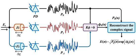
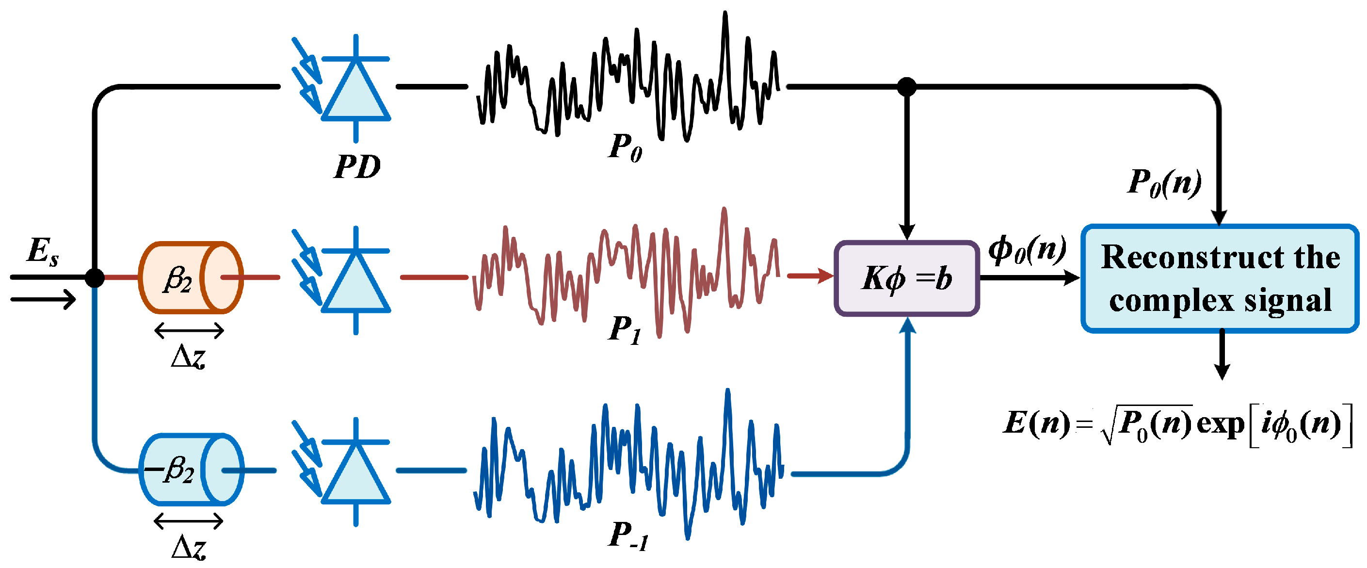
The reconstruction process of the complex signal, when the 2nd-order central difference approximation is employed for the derivative of intensity, is illustrated in Figure 1. The received signal is divided into three processing paths. One path is directly subjected to optoelectronic detection, while the other two paths traverse dispersive media with specified lengths of $\Delta z$ and group velocity dispersions of ${\beta }_2$ and $-{\beta }_2$ before undergoing optoelectronic detection. After passing through the dispersive media, both the intensity and phase of the signal are altered. However, the photodetector (PD) can only detect the intensity information. The variables $P_0$, $P_1$ and $P_{-1}$ represent the intensity curves extracted from the three signal paths. The discretized T-TIE can be rewritten as a linear matrix equation in the form of $K\varphi =b$, which we construct using the three sets of intensity information. By multiplying the column vector b with the inverse of the tridiagonal matrix K, we can obtain the column vector $\varphi$ composed of phase. Finally, by combining the initial intensity $P_0(n)$ with the recovered phase ${\varphi }_0(n)$, the complex signal is successfully reconstructed.

Figure 1. The process of reconstructing the complex signal based on the T-TIE.

When a signal propagates through the system, it is affected not only by amplified spontaneous emission (ASE) noise but also by electrical noise generated by the photodetector (PD) during optoelectronic conversion at the receiver. This electrical noise significantly degrades the accuracy of phase retrieval. Signals passing through different dispersive media are detected by separate PDs, leading to the introduction of uncorrelated electrical noise across distinct intensity signal paths. Consequently, this noise cannot be eliminated via simple subtraction. The 2nd-order central difference, after the introduction of electrical noise, can be expressed as

$${\displaystyle \frac{(P_{\Delta z}(n)+{\xi }_1)-(P_{-\Delta z}(n)+{\xi }_{-1})}{{\beta }_2\Delta z}}={\displaystyle \frac{P_{\Delta z}(n)-P_{-\Delta z}(n)}{{\beta }_2\Delta z}}+{\displaystyle \frac{{\xi }_1-{\xi }_{-1}}{{\beta }_2\Delta z}}$$

(5)

Here, ${\xi }_i$ represents the electrical noise power. The numerical value of the signal power difference term is small, making it highly sensitive to electrical noise. While reducing the dispersion value ${\beta }_2\Delta z$ makes the central difference approximation more accurate, it also increases the interference from electrical noise [18].

2.3. High-Order Difference Approximation of Intensity Derivatives

To solve for T-TIE, we need to obtain the 1st-order derivative of intensity with respect to dispersion. However, since the optical signal does not propagate strictly linearly over a short length $\Delta z$ of dispersive medium, the accuracy of the approximation can be enhanced by eliminating the influence of nonlinear high-order derivatives [19,20]. The intensity distribution of a single signal sample after passing through dispersive media of length $\Delta z$ can be expanded using the Taylor series:

$$P(\Delta z)=P(0)+{\displaystyle \frac{\Delta z}{1!}}{\displaystyle \frac{\partial P}{\partial z}}+{\displaystyle \frac{{(\Delta z)}^2}{2!}}{\displaystyle \frac{{\partial }^{2}P}{\partial z^2}}+{\displaystyle \frac{{(\Delta z)}^3}{3!}}{\displaystyle \frac{{\partial }^{3}P}{\partial z^3}}+{\displaystyle \frac{{(\Delta z)}^4}{4!}}{\displaystyle \frac{{\partial }^{4}P}{\partial z^4}}+\cdots$$

(6)

The zeroth-order term $P(0)$ represents the initial optical intensity, serving as the reference value for analyzing the changes in signal transmission through the dispersive medium. The 1st-order term reflects the linear variation in signal intensity along the dispersive medium. This fundamental linear trend of increase or decrease is the primary manner in which dispersion affects the signal. High-order derivatives describe more complex scenarios, serving as corrections to the 1st-order linear variation, and they gradually diminish in significance with increasing order. While low-order terms are typically sufficient to describe the basic propagation behavior of the signal, high-order terms can offer a more precise analysis.

By transforming the Taylor expansion of the intensity, we can obtain the approximation of the intensity derivative considering high-order components:

$${\displaystyle \frac{\partial P}{\partial z}}={\displaystyle \frac{P(\Delta z)-P(0)}{\Delta z}}-\left[{\displaystyle \frac{\Delta z}{2!}}{\displaystyle \frac{{\partial }^{2}P}{\partial z^2}}+{\displaystyle \frac{{(\Delta z)}^2}{3!}}{\displaystyle \frac{{\partial }^{3}P}{\partial z^3}}+{\displaystyle \frac{{(\Delta z)}^3}{4!}}{\displaystyle \frac{{\partial }^{4}P}{\partial z^4}}+\cdots \right]$$

(7)

$${\displaystyle \frac{\partial P}{\partial z}}={\displaystyle \frac{P(\Delta z)-P(-\Delta z)}{2\Delta z}}-\left[{\displaystyle \frac{{(\Delta z)}^2}{3!}}{\displaystyle \frac{{\partial }^{3}P}{\partial z^3}}+{\displaystyle \frac{{(\Delta z)}^4}{5!}}{\displaystyle \frac{{\partial }^{5}P}{\partial z^5}}+\cdots \right]$$

(8)

The forward difference form is used in Equation (7), whereas the central difference form appears in Equation (8). We adopt high-order finite difference approximations, taking into account some of the terms within the brackets, to minimize the error as much as possible. It can also be observed that the truncation error of the central difference method contains only even powers of $\Delta z$. This occurs because the central difference approximates the derivative at a specific point by utilizing function values that are equidistant from the initial position on both sides. The dispersion values on either side are opposite in sign. When performing operations on the Taylor series expansion, the odd powers are canceled out, leaving only the even powers to contribute to the truncation error. Consequently, for the same order of approximation, the central difference method provides a more accurate approximation than the forward difference method.

We have constructed a difference formula that can accurately approximate the derivative of the intensity function up to a specified order. This difference formula is expressed as

$${\displaystyle \frac{\partial P}{\partial z}}\approx {\displaystyle \frac{1}{\Delta z}}{\displaystyle \sum _{i=-m}^n{a}_{i}P(i\Delta z)}$$

(9)

Here, $a_i$ are undetermined coefficients, and $k=m+n$ is the order of the finite difference. For the forward difference, $m=0$ and $n=k$; for the central difference, $m=n=k/2$. By expanding the right side of the formula into a Taylor series and matching the corresponding orders, the value of $a_i$ can be determined. Table 1 lists the expressions for several different orders of forward and central differences.

Table 1. Approximation of the derivative for intensity with specified orders.

Forward Method		Centered Method
Order	Expression	Order	Expression
1st-order	${\displaystyle \frac{P_1-P_0}{\Delta z}}$	2nd-order	${\displaystyle \frac{P_1-P_{-1}}{2\Delta z}}$
2nd-order	${\displaystyle \frac{-P_2+4P_1-3P_0}{2\Delta z}}$	4th-order	${\displaystyle \frac{P_{-2}-8P_{-1}+8P_1-P_2}{12\Delta z}}$
3rd-order	${\displaystyle \frac{2P_3-9P_2+18P_1-11P_0}{6\Delta z}}$	6th-order	${\displaystyle \frac{P_{-3}-9P_{-2}+45P_{-1}-45P_1+9P_2-P_3}{60\Delta z}}$

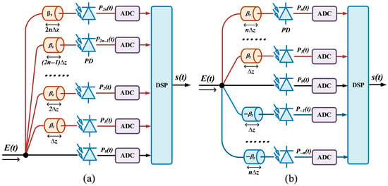
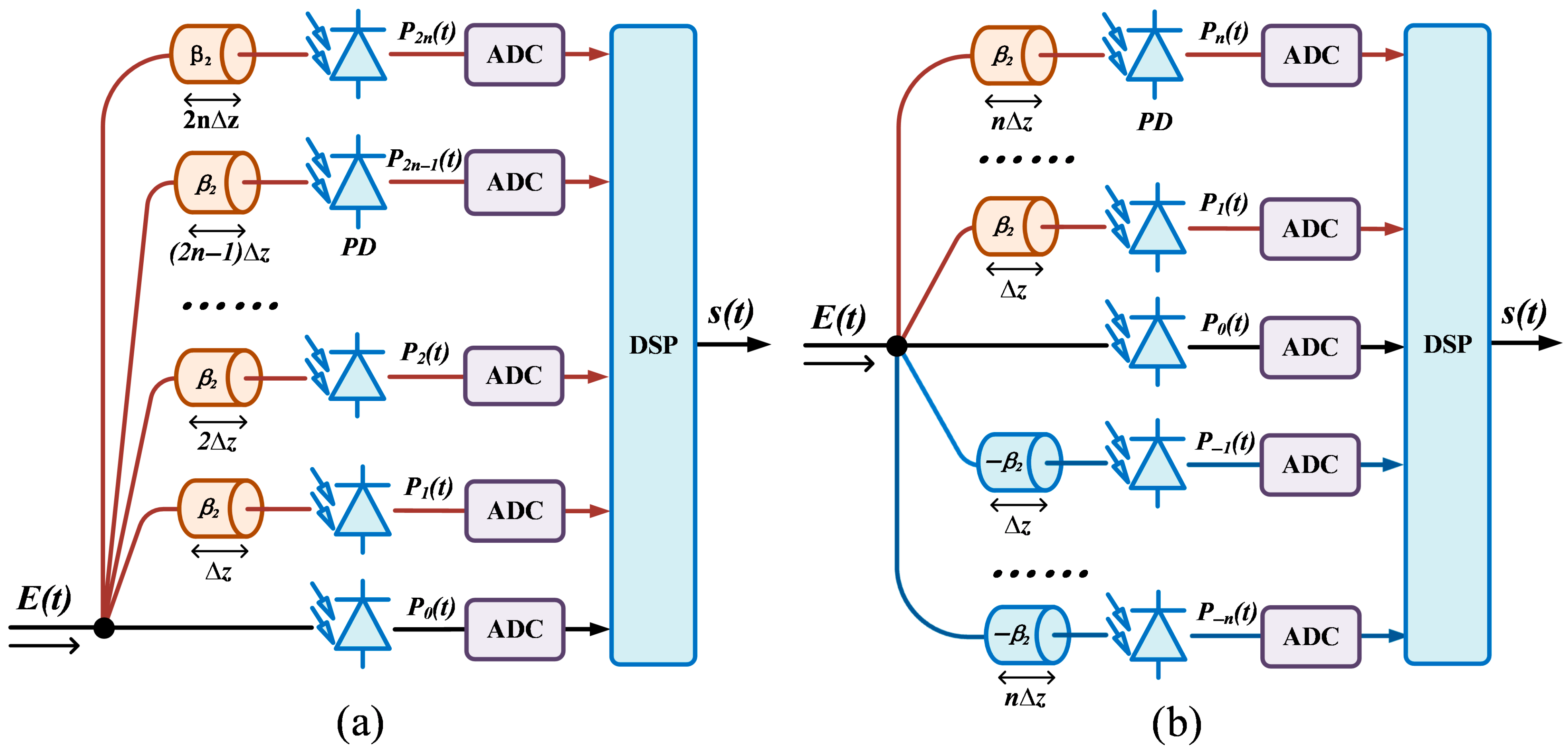
To implement high-order difference approximations, the received signal is propagated through dispersive media with different dispersion values, followed by separate photoelectric detection. Figure 2 illustrates the receiver structure. Figure 2a depicts the forward approach, which only requires measuring single-sided intensity information under positive GVD conditions. Figure 2b illustrates the central method, which necessitates acquiring double-sided intensity information for both positive and negative GVD values.

Figure 2. Receiver structure utilizing high-order difference approximations for the intensity derivative: (a) Forward method; (b) Centered method.

Multiple PDs are required to approximate the intensity derivative using high-order differences, and this introduces the challenge of additional noise. Furthermore, intensity components with larger weights tend to contribute more noise. As a result, high-order differences are more vulnerable to noise interference than low-order counterparts. Accordingly, we perform multiple intensity measurements for the signal path with the larger weight, and the average value of these measurements is used to construct the T-TIE. Given that the electrical noise in each measurement is random and exhibits both positive and negative fluctuations, averaging multiple intensity measurements (with superimposed electrical noise) enables partial cancelation of the positive and negative noise components.

3. Simulation Setup

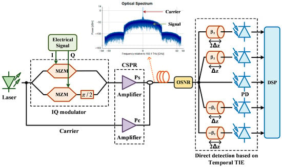
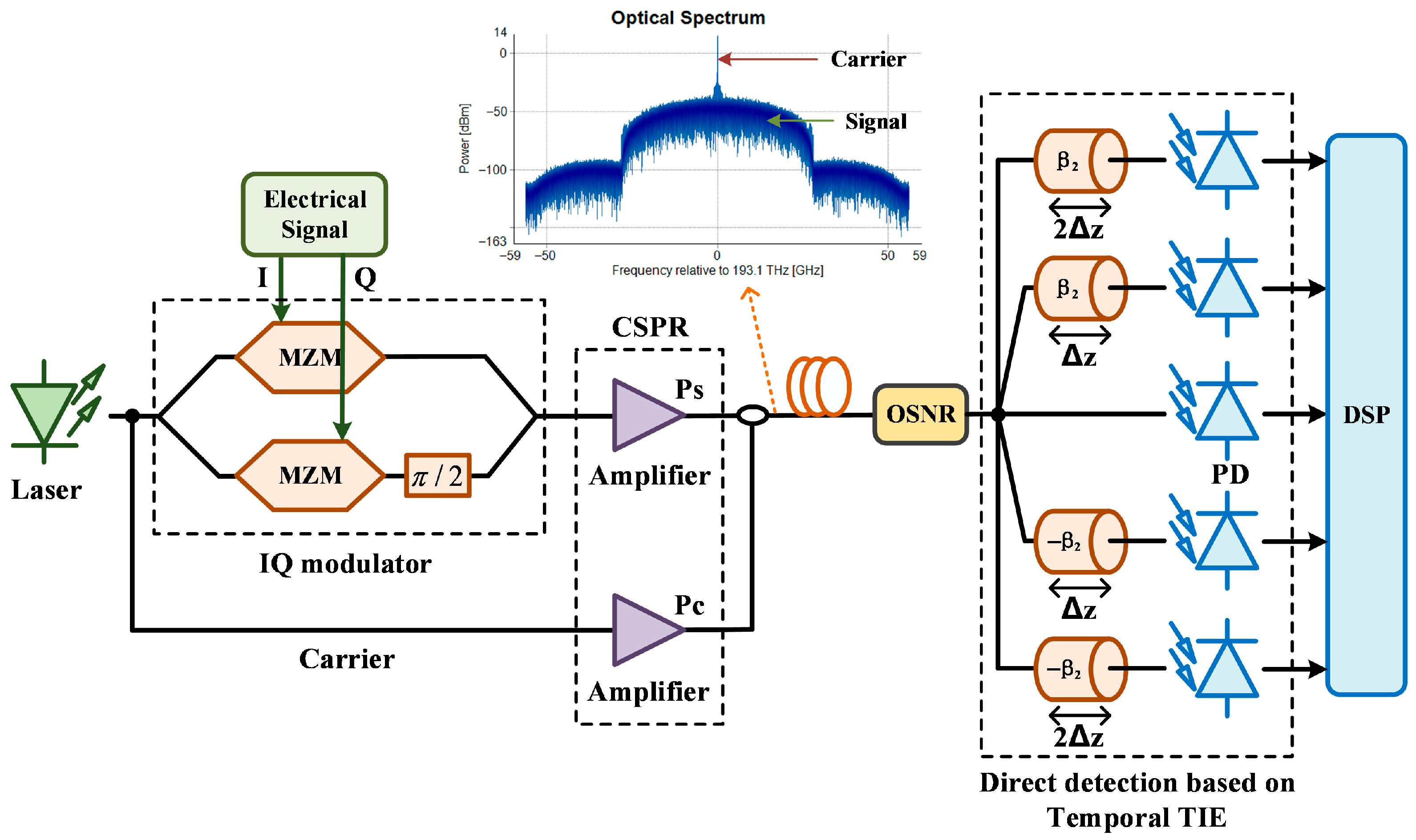
The schematic of the transmission system is depicted in Figure 3, where the intensity derivative with respect to dispersion is approximated using the 4th-order central difference method. A joint simulation was performed using VPI Transmission Maker (with its supporting tool VPIplayer 8.7) and MATLAB R2023a. A 28 GBaud single-carrier 16-quadrature amplitude modulation (16QAM) signal was transmitted through the system, with a total of 32,768 data symbols. A random binary sequence was generated in MATLAB, mapped to a 16QAM signal via Gray coding, and decomposed into in-phase (I) and quadrature (Q) components. In VPI, the signal was first upsampled by a factor of 4, followed by pulse shaping using a raised-cosine filter with a roll-off factor of 1. After digital-to-analog conversion (DAC), the electrical signal was converted to the optical domain using an in-phase and quadrature (IQ) modulator. The IQ modulator consists of two dual-drive Mach-Zehnder modulators (DD-MZMs) and a 90° phase shifter, with both DD-MZMs operating in push-pull mode to implement amplitude modulation.

Figure 3. Schematic diagram of the transmission system.

When the signal is modulated into the optical domain, its trajectory in the complex plane varies continuously around the origin. Occasionally, abrupt phase changes may occur when the signal power approaches or deviates from zero, and this can introduce significant errors in phase retrieval using the T-TIE matrix equation solving method. To address this issue, a carrier with the same polarization state as the signal and centered in its frequency spectrum is added to achieve smoother phase variations [16]. The simulation does not consider the impact of the laser linewidth. The monochromatic light source emitted from an ideal laser is split into two paths: one path is used for IQ modulation of the electrical signal, while the other path serves as the carrier added to the center of the signal spectrum. The carrier amplitude is also a key factor affecting phase retrieval performance. A relatively large CSPR can make the signal phase variation smoother, but it also leads to the signal being submerged in noise. Therefore, in the simulations, with the OSNR set to 34 dB, we set the CSPR to 11 dB to ensure optimal performance, which is effective within the dispersion range considered in this study. Although the T-TIE-based receiver requires an optimal CSPR that is 2–3 dB higher than that of the KK receiver, it obviates the need for single-sideband modulation of the signal [16].

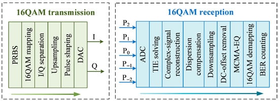
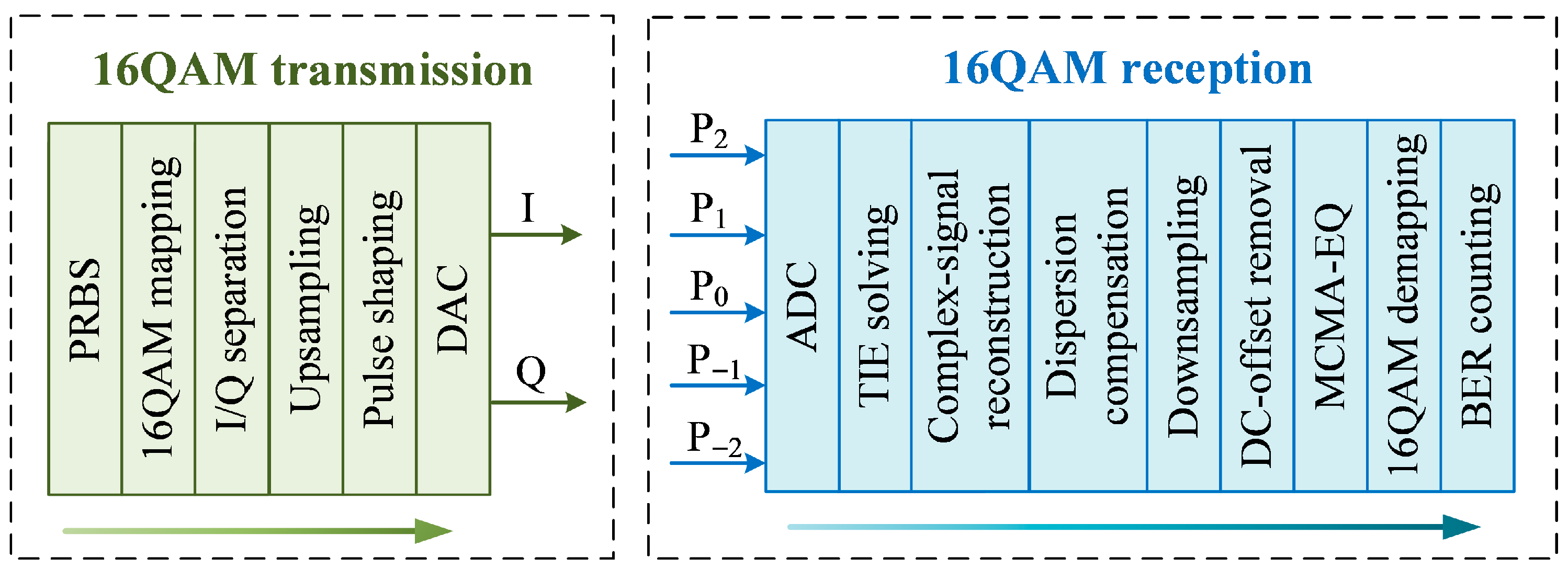
The signal is transmitted over a 100 km standard single-mode fiber (SSMF), with fiber chromatic dispersion and attenuation considered. Additionally, the signal is affected by amplified spontaneous emission (ASE) noise, and the corresponding optical signal-to-noise ratio (OSNR) is set to 34 dB. Ideal optoelectronic conversion efficiency is assumed for the PDs. The intensity signals acquired via photodetection are captured by oscilloscopes to construct the temporal transport-of-intensity equation (T-TIE). The phase is retrieved by solving the T-TIE, which is then combined with the original intensity $P_0$ to reconstruct the complex signal. Subsequently, chromatic dispersion in the fiber channel is compensated. The 4× oversampled signal is downsampled to 1×, followed by direct current (DC) removal and adaptive equalization using the modified constant modulus algorithm (MCMA). Finally, 16-quadrature amplitude modulation (16QAM) demapping is performed to calculate the bit error rate (BER). The digital signal processing (DSP) flows at the transmitter and receiver are illustrated in Figure 4.

Figure 4. DSP at the transmitting end and the receiving end.

4. Results and Discussion

4.1. Electric Noise’s Impact on Phase Recovery Performance

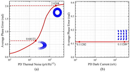
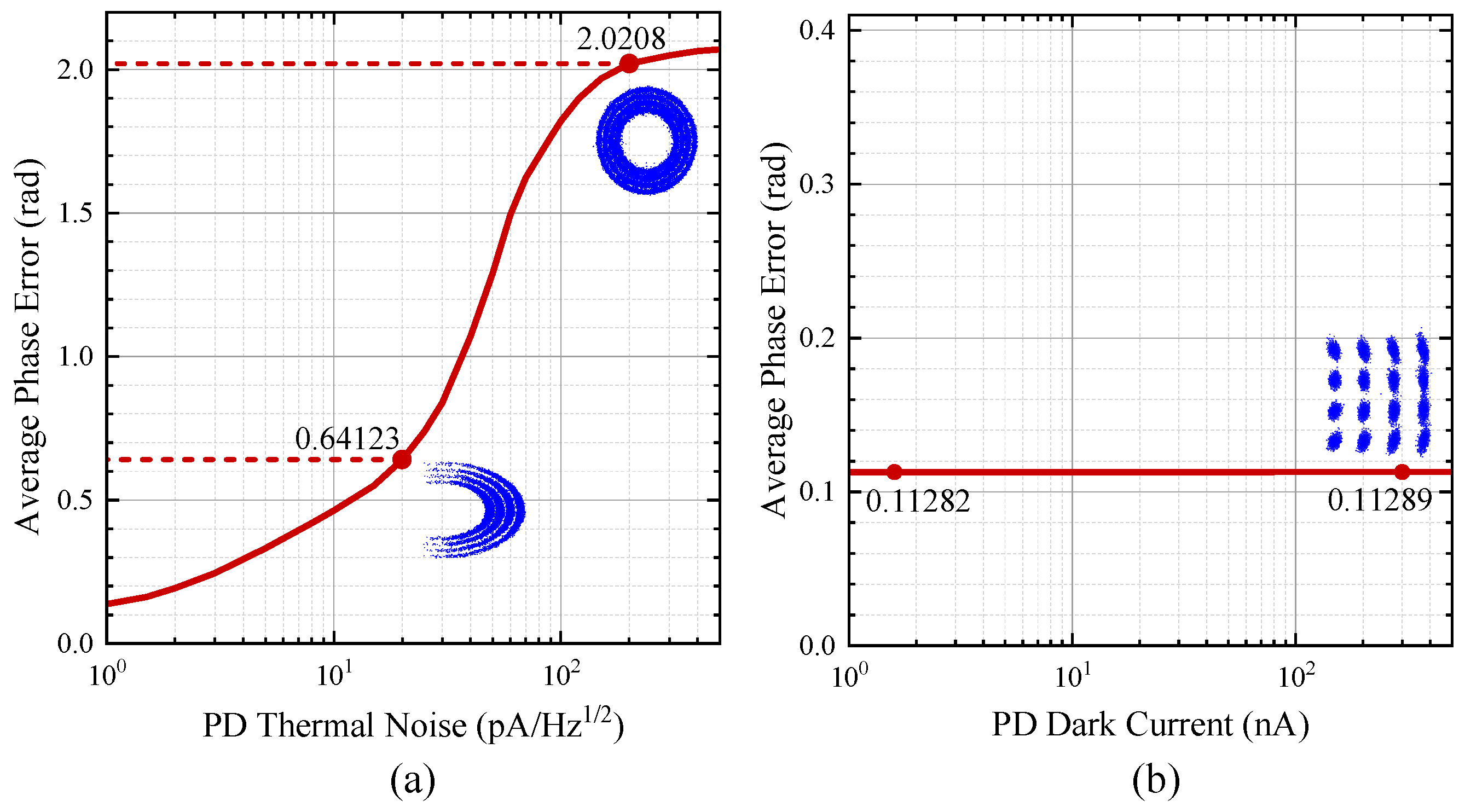
In optical fiber communication systems, signal transmission quality is affected by various types of electrical noise, which interfere with both the amplitude and phase of the signal. In this work, we analyzed the impacts of thermal noise and dark current on T-TIE-based phase retrieval performance. For the electrical noise analysis, the intensity derivative was approximated using the 2nd-order central difference method, and the dispersion value employed to solve the T-TIE was fixed at 180 ps/nm. The average phase error, denoted as $\Delta \phi ={\displaystyle \frac{1}{n}}{\displaystyle \sum _{i=1}^n\left|\phi (i)-{\phi }_0(i)\right|}$, is calculated by averaging the absolute differences between the recovered phase and the original phase. Herein, the recovered signal phase $\phi (i)$ refers to the phase after MCMA equalization, while the original signal phase ${\phi }_0(i)$ denotes the phase mapped to 16QAM. This metric is used to assess the quality of phase recovery.

Considering only thermal noise, Figure 5a shows how the average phase error varies with it. The increase in thermal noise leads to a more obvious phase deviation in the constellation diagram of the recovered signal. The average phase error increases gradually, and the peak value exceeds 2 radians, thus causing the original phase characteristics to be lost completely. Thermal noise refers to the random fluctuations in current caused by the thermal motion of electronic components within a receiver. This type of noise is characterized as a stationary Gaussian random process and is independent of optical intensity. When the signal is superimposed with this noise, both the amplitude and phase are affected, resulting in distortion of the complex signal [21].

Figure 5. The variation in average phase error under conditions of added electrical noise: (a) Thermal noise; (b) Dark current. (the blue part is the corresponding constellation diagram of the received signal).

With all other conditions held constant, only dark current was introduced without adding thermal noise, and Figure 5b illustrates how the average phase error of the recovered signal varies with dark current. As shown by the simulation results, the average phase error exhibits only minimal changes with increasing dark current, and the curve remains relatively flat. Furthermore, the average phase error across the entire dark current range is significantly smaller than that observed in the presence of thermal noise. Even when the dark current is increased to 300 nA, the constellation diagram of the recovered signal remains clear. Dark current is defined as the current generated by photodetectors due to thermal excitation of the material in the absence of incident light. The noise associated with dark current primarily manifests as a direct current (DC) offset in the signal, exerting a relatively minor impact on the alternating current (AC) component of the signal. Thus, the influence of dark current on the phase is negligible, and it will no longer be considered a major factor for discussion in subsequent simulations. Quantization noise is another key factor contributing to electrical noise in high-speed detectors and amplifiers, and the influence of quantization noise introduced during digital-to-analog converter/analog-to-digital converter (DAC/ADC) conversion on system performance is addressed in Section 4.3.

4.2. Comparison of Several Differential Methods

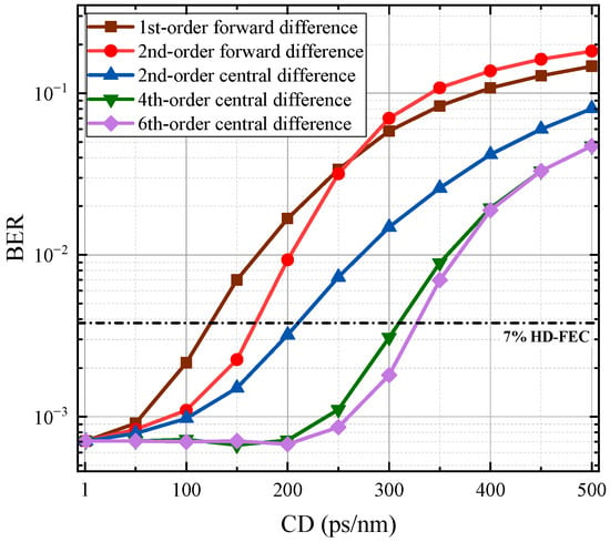
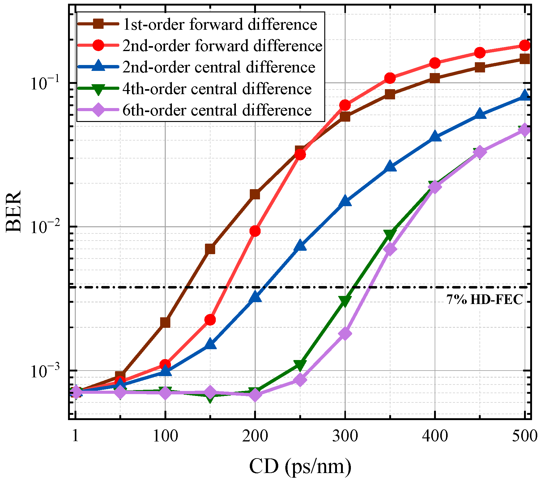
In the absence of any added electrical noise, we compared the signal recovery performance of forward difference versus central difference, and low-order difference versus high-order difference. As illustrated in Figure 6, for the same order (2nd-order), the BER of the central difference method is lower than that of the forward difference method across the entire dispersion range. This discrepancy arises because the truncation error of the central difference method does not include odd-power terms, thereby improving the approximation accuracy. When comparing central difference methods of different orders, the proposed 4th-order and higher-order methods exhibit a significant reduction in BER compared to the existing 2nd-order method. The 2nd-order central difference approximates the derivative using only two sets of intensity values, resulting in a 2nd-order truncation error [16]. In contrast, higher-order difference methods take full account of the influence of nonlinear factors, which effectively reduces the approximation error. As expected, increasing the order of the central difference method (e.g., to 6th-order) yields diminishing returns in terms of BER improvement, although it remains advantageous. Given that high-order methods require more components and complex calculations, central difference methods of 6th-order or higher will not be discussed further.

Figure 6. Variation in BER with dispersion under different differential methods.

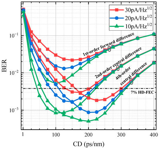
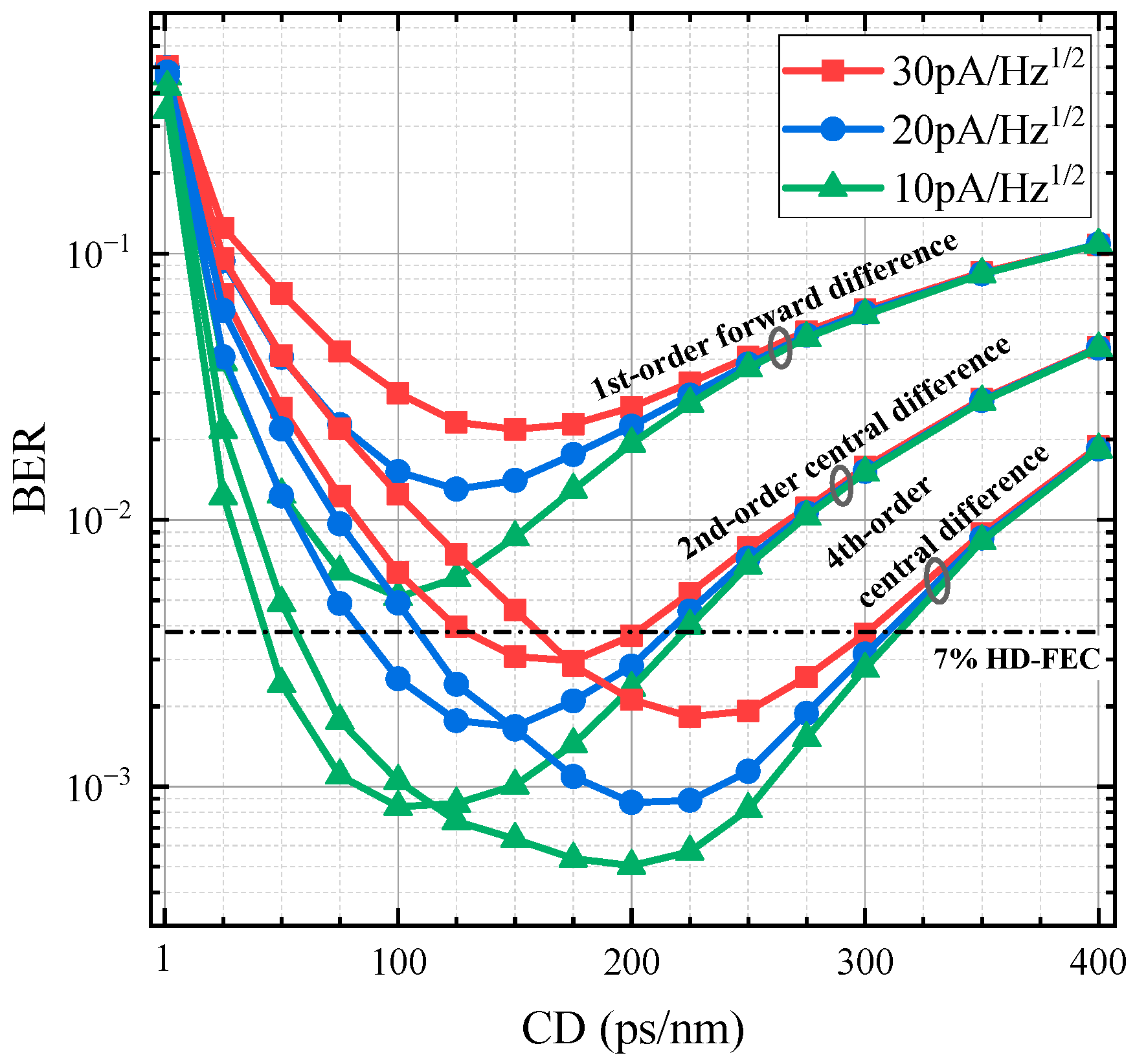
After introducing electrical noise, we compared different difference methods. The dark current was fixed at 10 nA, with a primary focus on analyzing the impact of thermal noise on phase retrieval performance. Figure 7 presents BER versus dispersion curves, comparing the traditional 1st-order forward difference method, the 2nd-order central difference method proposed by Masayuki Matsumoto, and the high-order (4th-order) central difference method. Thermal noise levels of 10 pA/Hz^1/2, 20 pA/Hz^1/2, and 30 pA/Hz^1/2, were evaluated—these values correspond to typical specifications of commercial photodiode-integrated transimpedance amplifiers (PIN-TIAs) and low-noise transimpedance amplifiers (e.g., ADN2880, OPA857).

Figure 7. After adding electrical noise, the impact of dispersion on BER under different differential methods.

Compared to the scenario without electrical noise, the introduction of thermal noise leads to a significant increase in BER at low dispersion values. Although the finite difference approximation error remains relatively small at these low dispersion levels, phase retrieval is highly sensitive to electrical noise. In contrast, at high dispersion values, phase retrieval becomes more robust to electrical noise; however, the reliability of the finite difference approximation decreases [17]. These two error sources are mutually conflicting, leading to the existence of an optimal dispersion value where both error types are relatively low, resulting in the minimum BER (defined herein as the optimal dispersion value). Furthermore, the higher the added thermal noise level, the larger the optimal dispersion value. This indicates that the high-order central difference can improve the approximation accuracy of the intensity derivative, and this advantage is more pronounced at higher dispersion values.

However, when the dispersion value is below a certain threshold, the BER with the 4th-order central difference method exceeds that with the 2nd-order under the same thermal noise. As shown in Table 1, in the 4th-order central difference method, the intensity values at positions $\Delta z$ and $-\Delta z$ are assigned a high weight of 8. As a result, the electrical noise introduced during photodetection is amplified eightfold. The high approximation accuracy of the 4th-order method fails to offset this noise amplification, leading to inferior performance.

4.3. Improved High-Order Differential Method

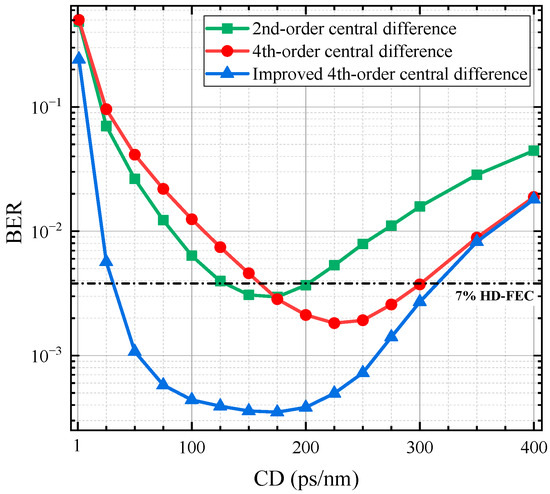
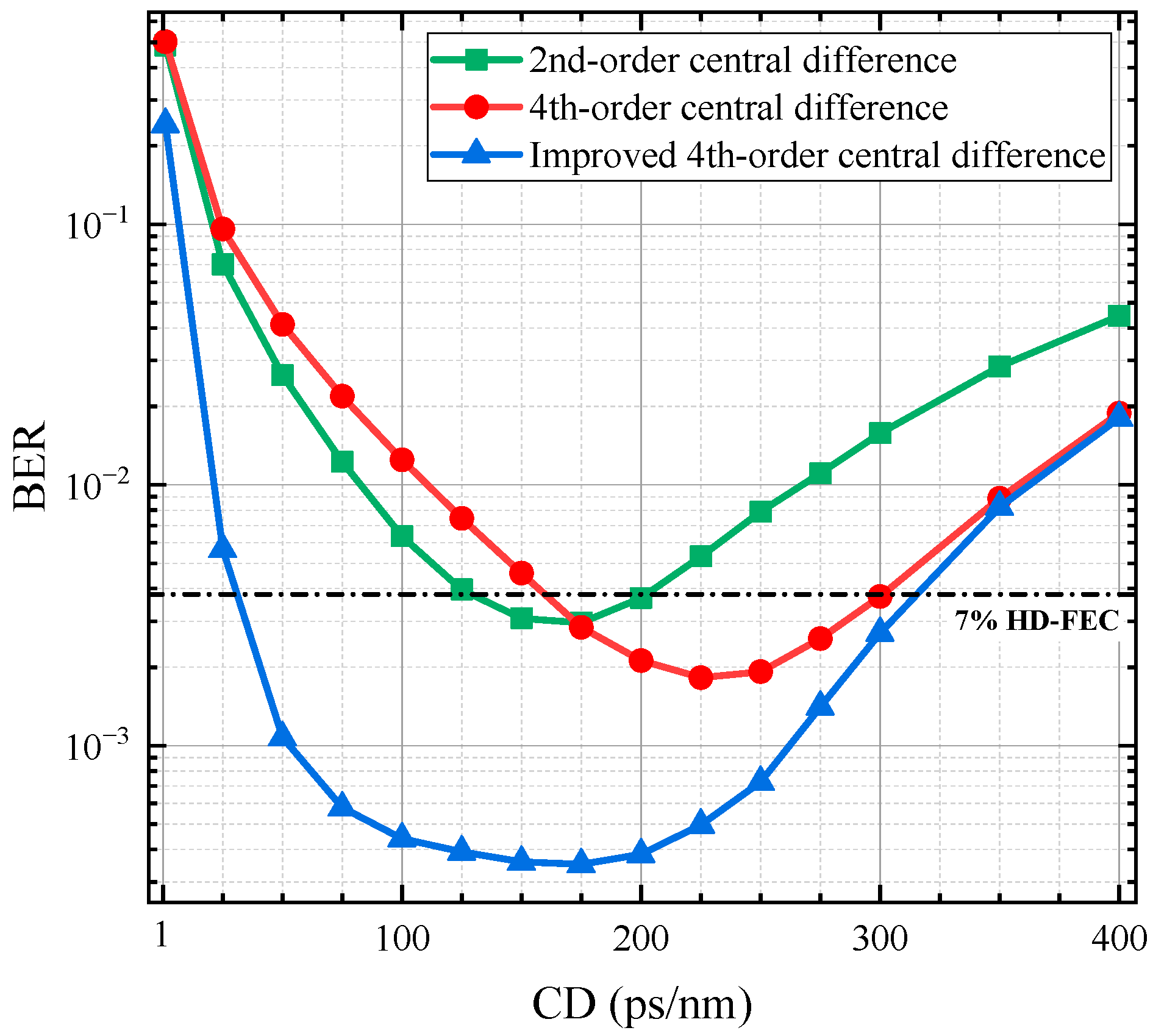
To address the issue that high-order differencing amplifies electrical noise interference, when using 4th-order central difference, we conducted eight measurements of the intensity at positions $\Delta z$ and $-\Delta z$, each with a different noise random seed for the PD. We then used the average of these eight measurements to solve for T-TIE. With the thermal noise set to 30 pA/Hz^1/2, we compared the BER of the improved 4th-order central difference method against that of single-measurement 4th-order and 2nd-order central difference methods, as demonstrated in Figure 8. At low dispersion values, the improved 4th-order central difference method shows a significant reduction in BER compared to the unimproved version, and it also exhibits a lower BER than that of the 2nd-order central difference method. In addition, the minimum BER at the optimal dispersion value is also reduced. Multiple intensity measurements do not show a significant improvement in performance at high dispersion values. This is because, at these levels, the finite difference approximation error is the dominant factor rather than electrical noise [16].

Figure 8. Comparison of multiple intensity measurements versus single intensity measurement under added electrical noise.

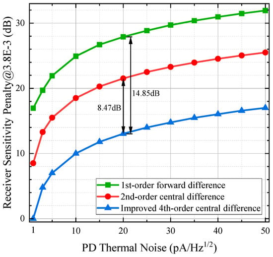
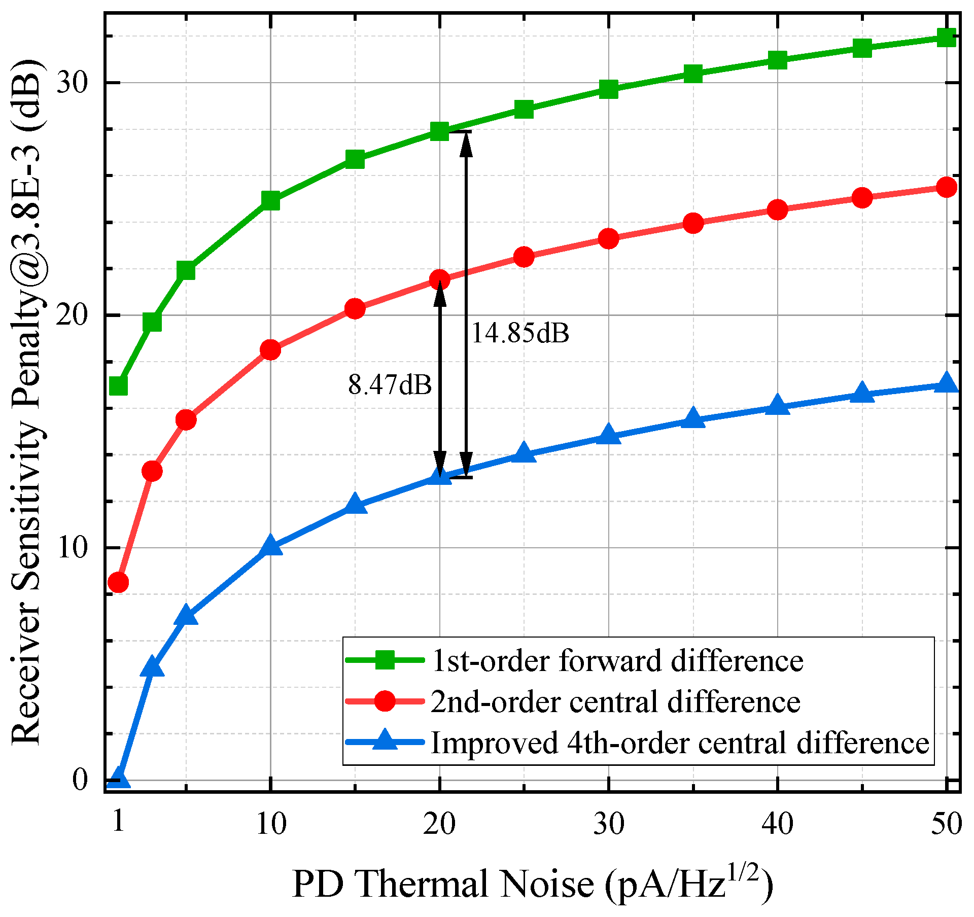
Under varying thermal noise levels, the optimal received optical power (ROP) for different difference methods varies with dispersion values, and each method exhibits a distinct optimal dispersion value. Measurements indicate that at the 7% HD-FEC threshold, the optimal dispersion values for the 1st-order forward difference, 2nd-order central difference, and improved 4th-order central difference methods are 90 ps/nm, 180 ps/nm, and 260 ps/nm, respectively. In subsequent simulations, each difference method was evaluated at its respective optimal dispersion value. The receiver sensitivity penalty curve is plotted in Figure 9, with the received optical power required for the improved 4th-order central difference method (under a thermal noise level of 1 pA/Hz^1/2 and a BER of 3.8 × 10⁻³) used as the baseline reference. Sensitivity penalty is defined as the difference in required received optical power relative to this baseline when either the difference scheme or thermal noise level is modified. It is evident that the improved 4th-order central difference method significantly enhances receiver sensitivity across all thermal noise levels. When the thermal noise is set to 20 pA/Hz^1/2, the improved 4th-order central difference method yields a receiver sensitivity gain of 8.47 dB compared with the 2nd-order central difference method, and a gain of 14.85 dB relative to the 1st-order forward difference method.

Figure 9. Receiver sensitivity penalty versus thermal noise for different differential methods.

We introduced real-valued Gaussian noise into each intensity signal in the simulation to emulate the impact of quantization noise on the signal. We use $SNR={\displaystyle \frac{⟨{\left[P_i(t)-⟨P_i(t)⟩\right]}^2⟩}{⟨n_i^2(t)⟩}}$ to represent the interference level of noise on signal fluctuations, where $P_i(t)$ denotes the detected intensity signals, $n_i(t)$ is the real-valued Gaussian noise added to $P_i(t)$, and $⟨•⟩$ represents average. We use $ENOB={\displaystyle \frac{SNR[dB]-1.76}{6.02}}$ to quantify the effective precision loss caused by quantization noise.

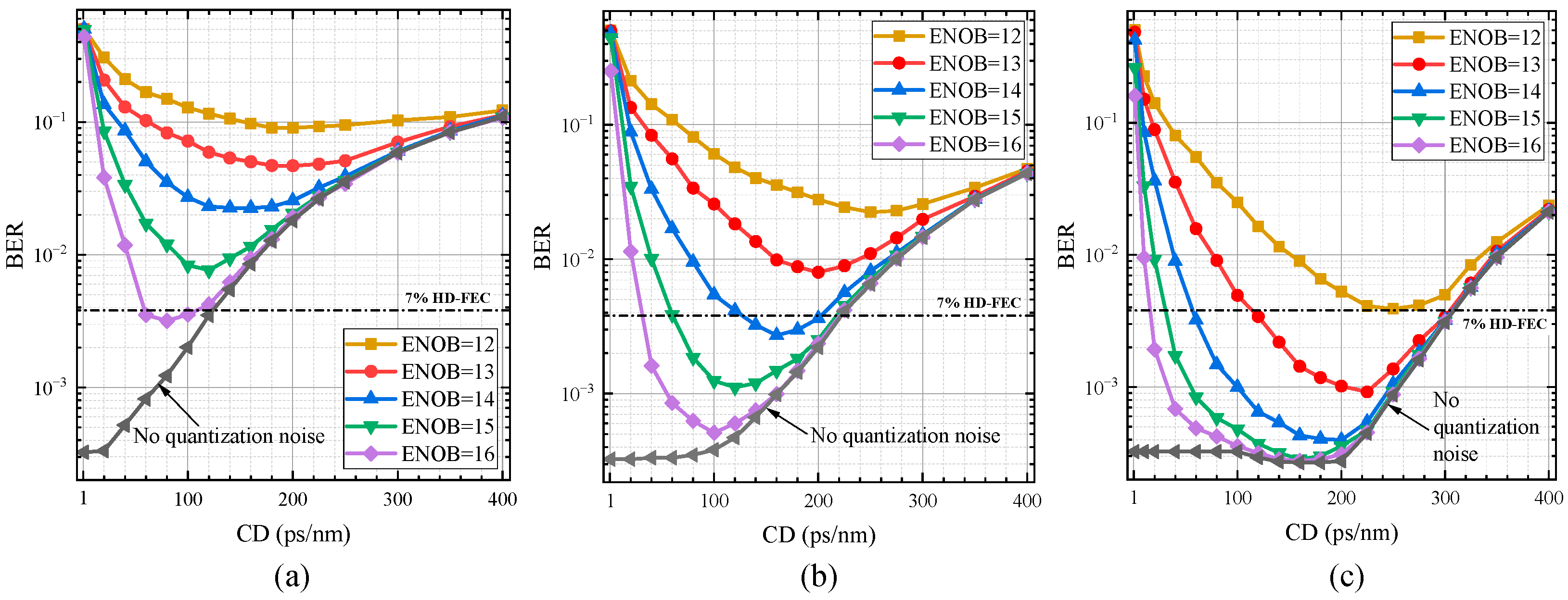
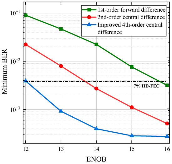
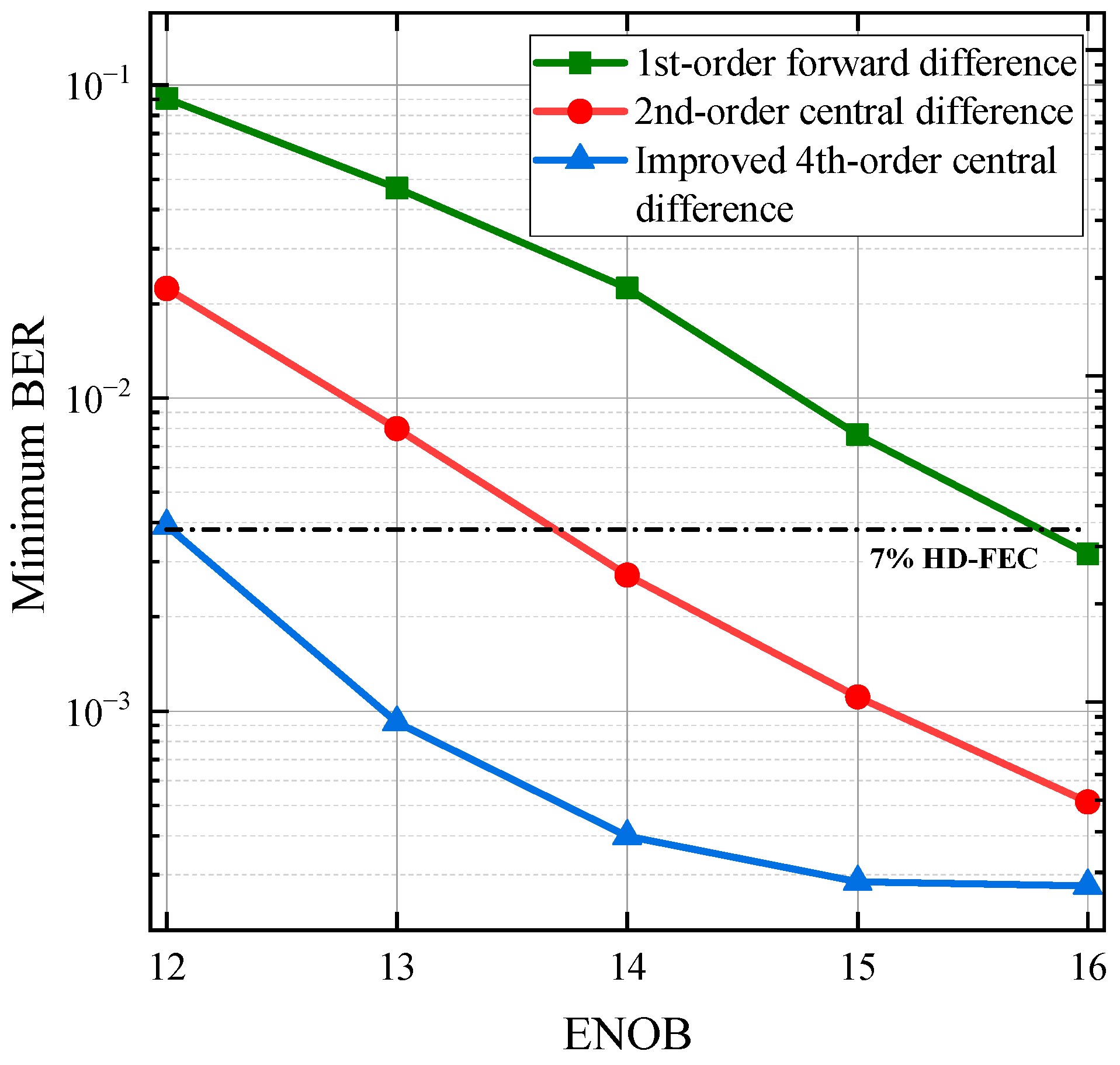
We measured the BER variation with chromatic dispersion (CD) under different ENOB conditions, as shown in Figure 10. When quantization noise is absent, a smaller CD value leads to more reasonable finite-difference approximations and lower BER. The 1st-order forward difference exhibits a significant BER increase at approximately CD = 20 ps/nm, while the 2nd-order central difference shows gradual BER degradation around CD = 100 ps/nm. The improved 4th-order central difference maintains stable performance until CD = 200 ps/nm. This behavior occurs because higher-order difference schemes allow larger step sizes (CD values) when approximating intensity derivatives. When recovering phase by solving the T-TIE, larger CD values are beneficial for tolerating quantization noise. Our primary focus is the minimum BER achievable at the optimal CD value. We measured the lowest attainable BER for these three difference schemes under varying ENOB, as illustrated in Figure 11. To achieve a 7% HD-FEC threshold, the required ENOB is approximately 16 for the 1st-order forward difference scheme, exceeds 13.5 for the 2nd-order central difference, and reduces to 12 for our improved 4th-order central difference method. This indicates that, compared with the existing methods, our method improves the tolerance to quantization noise by enhancing the approximation accuracy of the finite difference and balancing the uncorrelated noise among various branches.

Figure 10. Relationship between reconstruction performance and CD in the presence of quantization noise. Intensity derivatives approximated by (a) 1st-order forward difference, (b) 2nd-order central difference, and (c) improved 4th-order central difference.

Figure 11. Relationship between minimum BER and ENOB.

Although our method achieves better signal recovery performance than low-order difference methods, it is still highly necessary to further improve the electrical noise tolerance of the phase retrieval approach based on the T-TIE. Moving forward, continuous refinement of the discretization algorithm and optimization of the receiver architecture can be carried out. In addition, future research may explore potential extensions of the proposed framework: integrating the developed difference scheme with carrier-assisted techniques [22,23] to enhance low dispersion noise robustness, and exploring spatial-degree-of-freedom-based phase retrieval in multi-core fibers by leveraging polarization diversity insights from recent receivers for more comprehensive complex signal recovery [24,25].

5. Conclusions

In this study, we investigated the effects of PD thermal noise and dark current on T-TIE-based phase retrieval performance. Our results demonstrate that dark current exerts a negligible influence on the signal, whereas thermal noise significantly degrades phase retrieval. Additionally, the finite difference approximation error of the intensity derivative is a critical factor governing phase retrieval accuracy. By utilizing high-order difference approximations for the intensity derivative, which account for the influence of nonlinear factors more comprehensively, we effectively reduced approximation errors at high dispersion values. Furthermore, we found that for methods of the same order, the truncation error of the central difference method is lower than that of the forward difference method, thereby further improving approximation accuracy.

To address the issue that high-order differences are more susceptible to electrical noise at low dispersion values, we employed a method of averaging multiple measurements of high-weight intensity values to balance noise levels. Simulation results show that, compared with the 1st-order forward difference and 2nd-order central difference methods, the improved 4th-order central difference method proposed in this study achieves superior recovery performance for signals affected by electrical noise.

References

- Zhong, K.; Zhou, X.; Huo, J.; Yu, C.; Lu, C.; Lau, A.P.T. Digital signal processing for short-reach optical communications: A review of current technologies and future trends. J. Light. Technol. 2018, 36, 377–400. [Google Scholar] [CrossRef] [Scilit]
- Qiao, Z.; Yao, Y.; Wang, X.; Fan, W.; Lin, Z. Single-shot full-field characterization of short pulses by using temporal annealing modified Gerchberg–Saxton algorithm. J. Light. Technol. 2017, 35, 2541–2547. [Google Scholar] [CrossRef] [Scilit]
- Chen, H.; Fontaine, N.K.; Gené, J.M.; Ryf, R.; Neilson, D.; Raybon, G. Full-field, carrier-less, polarization-diversity, direct detection receiver based on phase retrieval. In Proceedings of the 45th European Conference on Optical Communication (ECOC), Dublin, Ireland, 22–26 September 2019; pp. 1–3. [Google Scholar]
- Chen, H.; Huang, H.; Fontaine, N.K.; Ryf, R. Phase retrieval with fast convergence employing parallel alternative projections and phase reset for coherent communications. Opt. Lett. 2020, 45, 1188–1191. [Google Scholar] [CrossRef] [Scilit] [PubMed]
- Karar, A.S. Iterative algorithm for electronic dispersion compensation in IM/DD systems. J. Light. Technol. 2019, 38, 698–704. [Google Scholar] [CrossRef] [Scilit]
- Li, Z.; Erkılınç, M.S.; Shi, K.; Sillekens, E.; Galdino, L.; Thomsen, B.C.; Bayvel, P.; Killey, R.I. SSBI mitigation and the Kramers–Kronig scheme in single-sideband direct-detection transmission with receiver-based electronic dispersion compensation. J. Light. Technol. 2017, 35, 1887–1893. [Google Scholar] [CrossRef] [Scilit]
- Mecozzi, A.; Antonelli, C.; Shtaif, M. Kramers–Kronig coherent receiver. Optica 2016, 3, 1220–1227. [Google Scholar] [CrossRef] [Scilit]
- Zuo, C.; Li, J.; Sun, J.; Fan, Y.; Zhang, J.; Lu, L.; Zhang, R.; Wang, B.; Huang, L.; Chen, Q. Transport of intensity equation: A tutorial. Opt. Lasers Eng. 2020, 135, 106187. [Google Scholar] [CrossRef] [Scilit]
- Teague, M.R. Irradiance moments: Their propagation and use for unique retrieval of phase. J. Opt. Soc. Am. 1982, 72, 1199–1209. [Google Scholar] [CrossRef] [Scilit]
- Teague, M.R. Deterministic phase retrieval: A Green’s function solution. J. Opt. Soc. Am. 1983, 73, 1434–1441. [Google Scholar] [CrossRef] [Scilit]
- Streibl, N. Phase imaging by the transport equation of intensity. Opt. Commun. 1984, 49, 6–10. [Google Scholar] [CrossRef] [Scilit]
- Dorrer, C. Characterization of nonlinear phase shifts by use of the temporal transport-of-intensity equation. Opt. Lett. 2005, 30, 3237–3239. [Google Scholar] [CrossRef] [Scilit] [PubMed]
- Matsumoto, M. A phase retrieval method using dispersion for direct detection of biased QAM signals. In Proceedings of the 2018 Conference on Lasers and Electro-Optics (CLEO), San Jose, CA, USA, 13–18 May 2018; pp. 1–2. [Google Scholar]
- Xiang, Y.; Tang, M.; Tan, H.; Wang, L.; Chen, Y.; Fu, S. Complex signal reconstruction in direct-detection OFDM by solving temporal transport-of-intensity equation. In Proceedings of the 2020 Asia Communications and Photonics Conference (ACP) and International Conference on Information Photonics and Optical Communications (IPOC), Beijing, China, 24–27 October 2020; pp. 1–3. [Google Scholar]
- Xiang, Y.; Chen, Y.; Chen, J.; Wang, L.; Jiang, T.; Tang, M. Phase retrieval of complex OFDM signal by solving temporal transport-of-intensity equation. IEEE Photon. Technol. Lett. 2021, 33, 1006–1009. [Google Scholar] [CrossRef] [Scilit]
- Matsumoto, M. Optical signal phase reconstruction based on temporal transport-of-intensity equation. J. Light. Technol. 2020, 38, 4722–4729. [Google Scholar] [CrossRef] [Scilit]
- Matsumoto, M. Complex field reconstruction of optical OFDM signals based on temporal transport-of-intensity equation. Opt. Express 2021, 29, 36155–36166. [Google Scholar] [CrossRef] [Scilit] [PubMed]
- Matsumoto, M. Influence of electrical noise on temporal optical phase reconstruction using transport-of-intensity equation. In Proceedings of the 2020 IEEE Photonics Society Summer Topicals Meeting Series (SUM), Cabo San Lucas, Mexico, 13–15 July 2020; pp. 1–2. [Google Scholar]
- Soto, M.; Acosta, E. Improved phase imaging from intensity measurements in multiple planes. Appl. Opt. 2007, 46, 7978–7981. [Google Scholar] [CrossRef] [Scilit] [PubMed]
- Waller, L.; Tian, L.; Barbastathis, G. Transport of intensity phase-amplitude imaging with high order intensity derivatives. Opt. Express 2010, 18, 12552–12561. [Google Scholar] [CrossRef] [Scilit] [PubMed]
- Kasper, B.L.; Mizuhara, O.; Chen, Y.-K. High bit-rate receivers, transmitters, and electronics. In Optical Fiber Telecommunications IV-A; Academic Press: Cambridge, MA, USA, 2002; pp. 784–851. [Google Scholar]
- Wu, Q.; Zhu, Y.; Hu, W. Carrier-assisted phase retrieval. J. Light. Technol. 2022, 40, 5583–5596. [Google Scholar] [CrossRef] [Scilit]
- Wu, Q.; Zhu, Y.; Zhuge, Q.; Hu, W. Dual-carrier-assisted phase retrieval for polarization division multiplexing. J. Light. Technol. 2022, 40, 7297–7306. [Google Scholar] [CrossRef] [Scilit]
- Wu, Q.; Zhu, Y.; Li, X.; Jiang, H.; Cheng, C.; Fu, M.; Zhang, Y.; Zhuge, Q.; Li, Z.; Hu, W. Four-dimensional direct detection receiver enabling Jones-space field recovery with phase and polarization diversity. Photonics Res. 2024, 12, 399–410. [Google Scholar] [CrossRef] [Scilit]
- Wu, Q.; Ribezzo, D.; Di Sciullo, G.; Cocchi, S.; Shaji, D.A.; Zischler, L.A.; Luis, R.; Serena, P.; Lasagni, C.; Bononi, A.; et al. Integration of quantum key distribution and high-throughput classical communications in field-deployed multi-core fibers. Light Sci. Appl. 2025, 14, 274. [Google Scholar] [CrossRef] [Scilit] [PubMed]
Disclaimer/Publisher’s Note: The statements, opinions and data contained in all publications are solely those of the individual author(s) and contributor(s) and not of MDPI and/or the editor(s). MDPI and/or the editor(s) disclaim responsibility for any injury to people or property resulting from any ideas, methods, instructions or products referred to in the content. |
© 2025 by the authors. Licensee MDPI, Basel, Switzerland. This article is an open access article distributed under the terms and conditions of the Creative Commons Attribution (CC BY) license.