Research on Anomaly Detection and Correction Methods for Nuclear Power Plant Operation Data

Abstract

The data collection and analytical capabilities of the Instrumentation and Control (I&C) system in nuclear power plants (NPPs) continue to advance, thereby enhancing operational state awareness and enabling more precise control. However, the data acquisition, transmission, and storage devices in nuclear power plant (NPP) I&C systems typically operate in harsh environments. This exposure can lead to device failures and susceptibility to external interference, potentially resulting in data anomalies such as missing samples, signal skipping, and measurement drift. This paper presents a Gated Recurrent Unit and Multilayer Perceptron (GRU-MLP)-based method for anomaly detection and correction in NPP I&C system data. The goal is to improve operational data quality, thereby supplying more reliable input for system analysis and automatic controllers. Firstly, the short-term prediction algorithm of operation data based on the GRU model is studied to provide a reference for operation data anomaly detection. Secondly, the MLP model is connected to the GRU model to recognize the difference between the collected value and the prediction value so as to distinguish and correct the anomalies. Finally, a series of experiments were conducted using operational data from a pressurized water reactor (PWR) to evaluate the proposed method. The experiments were designed as follows: (1) These experiments assessed the model’s prediction performance across varying time horizons. Prediction steps of 1, 3, 5, 10, and 20 were configured to verify the accuracy and robustness of the data prediction capability over short and long terms. (2) The model’s effectiveness in identifying anomalies was validated using three typical patterns: random jump, fixed-value drift, and growth drift. The growth drift category was further subdivided into linear, polynomial, and logarithmic growth to comprehensively test detection performance. (3) A comparative analysis was performed to demonstrate the superiority of the proposed GRU-MLP algorithm. It was compared against the interactive window center value method and the ARIMA algorithm. The results confirm the advantages of the proposed method for anomaly detection, and the underlying reasons are analyzed. (4) Additional experiments were carried out to discuss and verify the mobility (or transferability) of the prediction algorithm, ensuring its applicability under different operational conditions.

1. Introduction

The digitization of nuclear power plant (NPP) Instrumentation and Control (I&C) systems has led to advanced data analysis and processing capabilities for assessing operational status. These capabilities facilitate both online functions—such as real-time fault diagnosis, equipment monitoring, and operational decision support—and offline applications, including experience feedback, maintenance planning, and aging management [1]. Consequently, the availability of high-quality operational data is essential for the effectiveness of these applications.

However, sensors and data acquisition equipment in nuclear power plant (NPP) Instrumentation and Control (I&C) systems often operate in adverse environments and are susceptible to strong external interference, which can lead to performance degradation or malfunction. Consequently, data quality issues such as missing values and signal drift are frequently observed in NPP operational data. This, in turn, causes a significant portion of the measured data to deviate from the true values, thereby compromising the accuracy of subsequent data analysis. Inaccurate operational data analysis can consequently lead to the misjudgment of equipment status. Therefore, it is essential to develop effective anomaly detection and correction algorithms for NPP operational data to assist operators in making accurate assessments of the plant’s condition. Furthermore, the corrected data can be fed into the automatic control system. This prevents improper control actions triggered by erroneous data and contributes to fault-tolerant control.

A common anomaly detection method employs a predictive model. By comparing the predicted and observed values at each sampling point, an observed value is identified as an outlier when their discrepancy exceeds a set threshold. Therefore, it is imperative to develop feasible and efficient methods for predicting operational parameters. Accurate predictions provide a foundational reference for anomaly detection [2]. Existing approaches encompass a range of algorithms, including those based on statistics [3,4], similarity [5,6,7,8,9,10], machine learning [11,12], and deep learning [13,14,15].

The rapid advancement of artificial intelligence (AI) has spurred growing interest in intelligent algorithms for data prediction and anomaly detection in nuclear power plants (NPPs). Early research in this field predominantly relied on methods grounded in expert knowledge and mathematical models. For instance, Sun Yingjie et al. employed the Multivariable State Estimation Technique (MSET) and the Sequential Probability Ratio Test (SPRT) for system variable estimation and anomaly judgment [16]. Similarly, Gao Zhengxin conducted a review of prediction methods for NPP state trends [17]. Zhao Mengwei et al. designed a reactor power controller using a single-step predictive control scheme integrated with online Takagi–Sugeno (T-S) fuzzy identification and a particle swarm optimization algorithm. The proposed controller demonstrated superior performance in terms of response speed and overshoot suppression compared to the conventional PI control method [18].

Driven by continuous innovations in machine learning and deep learning, data-driven methods have garnered significant research attention. For instance, Xu Yanshun employed a genetic algorithm to optimize the parameters of a Support Vector Regression (SVR) model for fault prediction in nuclear power plants (NPPs) [19]. Addressing the issue of slow convergence in Artificial Neural Networks (ANNs), Jiang Botao et al. analyzed the characteristics of nuclear power variations under accident conditions. They subsequently proposed two distinct prediction methods: one for nuclear power based on ν-Support Vector Regression (ν-SVR), and another for critical heat flux based on Gaussian Process Regression (GPR) [20,21]. Artificial Neural Networks (ANNs) represent one of the most extensively studied methods in this domain. Yu Ren et al. developed a monitoring method for abnormal operational states in NPPs based on a dynamic Hopfield neural network, demonstrating its strong capability in detecting anomalous parameter changes [1]. Lei Jicong et al. evaluated several models—including linear regression, regression tree, Multilayer Perceptron (MLP), and random forest—for predicting the nucleon density of various nuclides in a reactor. Using multiple quantitative evaluation metrics, they concluded that the MLP model delivered the best performance [22]. Furthermore, Zhang Siyuan et al. proposed a multi-feature fusion, multi-step state prediction model based on the Long Short-Term Memory (LSTM) network for NPP operational parameters and verified its practicality [23].

This work proposes an integrated method for operation data prediction, anomaly detection and correction for NPPs based on the fusion model of Gated Recurrent Unit and Multilayer Perceptron (GRU-MLP). Its main contributions are as follows:

(1)

A GRU-MLP-model-based NPP parameter prediction, anomaly detection and real-time correction algorithm is designed, and its feasibility is verified.

(2)

The algorithm flow based on the anomaly detection and correction model is designed so as to improve the prediction accuracy of GRU prediction algorithm for the operation data containing anomalies.

(3)

The nonlinear fitting ability of MLP model is used to optimize the fixed threshold determination method within the prediction–anomaly–detection mechanism, and the accuracy of anomaly diagnosis with the mechanism is improved.

(4)

The migration ability of GRU model applied to NPP prediction function is discussed and verified.

2. The Principle of the Algorithm

The fundamental anomaly detection strategy employed in this work is based on comparing the residuals—the differences between the predicted and observed values. A data point is flagged as anomalous if its residual exceeds a predetermined threshold. Consequently, the proposed algorithm is structured into two sequential stages: “prediction” and “detection.” The prediction stage utilizes a Gated Recurrent Unit (GRU) model, while the detection stage is accomplished using a Multilayer Perceptron (MLP) model. The principles of these two stages are elaborated upon below.

2.1. Principle of the Prediction Stage

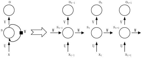
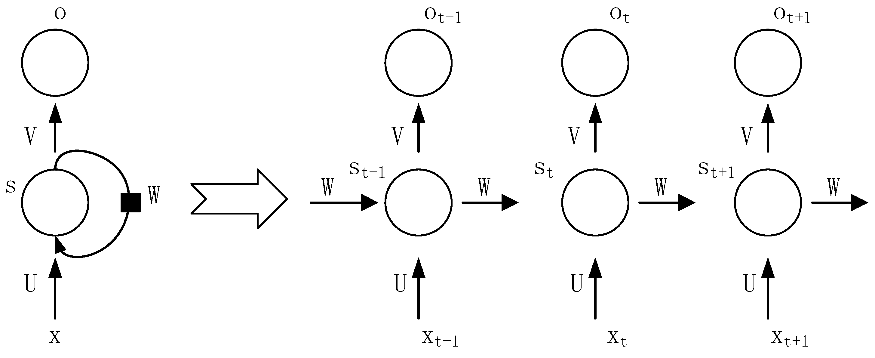
The prediction of NPP operational parameters serves two primary purposes: to provide a reference for detecting anomalies in the collected parameter values, and to facilitate the correction of data identified as outliers. The core algorithm chosen for the prediction stage is the Recurrent Neural Network (RNN). This selection is justified by the fact that NPP operational data constitute a characteristic time series, a data structure for which RNNs are particularly well-suited. Modeling NPP operational data requires the capability to process both current and historical information within the time series simultaneously. However, commonly used Artificial Neural Networks (ANNs), such as Deep Neural Networks (DNNs) and Convolutional Neural Networks (CNNs), are typically based on a feedforward architecture where signals propagate sequentially through the network. This inherent structure limits their effectiveness in directly capturing temporal dependencies. This architecture is inherently limited to processing finite, fixed-length inputs and cannot propagate information across time steps. Consequently, it is ill-suited for time series data, where temporal dependencies are critical [24,25]. In contrast, Recurrent Neural Networks (RNNs) demonstrate a superior capability for modeling sequential data, achieving outstanding performance in prediction tasks [26]. RNNs possess a recurrent architecture that allows them to incorporate information from both the current input and their own previous state. This ability to process sequences step-by-step frees them from the constraint of fixed-length inputs, enabling more dynamic modeling of sequential data. The operating principle is illustrated in Figure 1.

Figure 1. Schematic diagram of RNN principle.

However, standard RNNs suffer from the vanishing and exploding gradient problems when processing long sequences. To mitigate these issues, gating mechanisms were introduced to regulate the information flow and control the influence of historical information on the current output. Consequently, advanced variants such as the Long Short-Term Memory (LSTM) and the Gated Recurrent Unit (GRU) networks have been developed, which incorporate these gates to model long-range dependencies effectively.

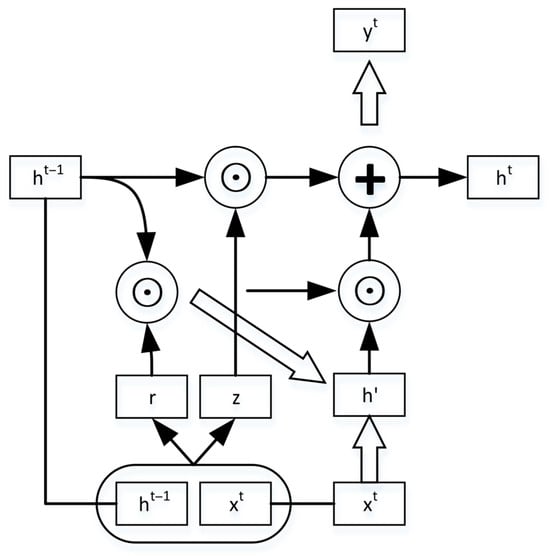
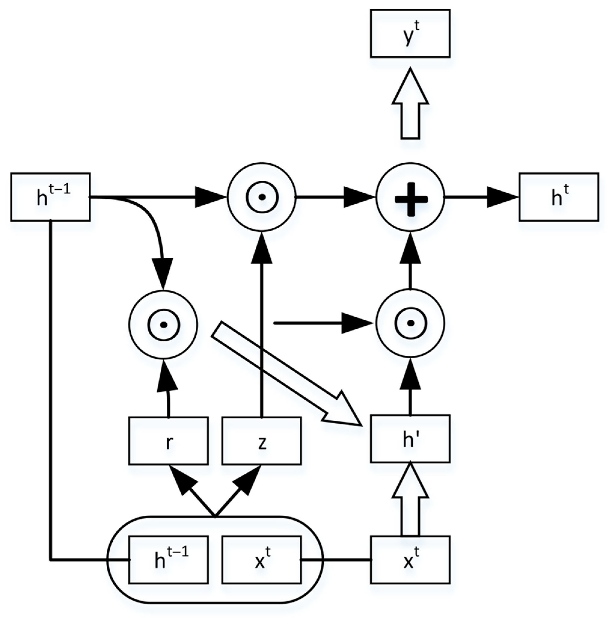
Figure 2 and Figure 3 are the principal diagrams of GRU and LSTM, respectively. “⊙” represents multiplication of matrix elements, and “+” represents matrix addition. The input of the gate control unit includes the data input vector x^t at the current moment and the history vector h^t−1 transmitted from the former node, which contains the historical information. Combining x^t and h^t−1, the output y^t of the current hidden node and the hidden state h^t transmitted to the next node can be obtained through the operation of the gate control unit.

Figure 2. Principal diagram of GRU.

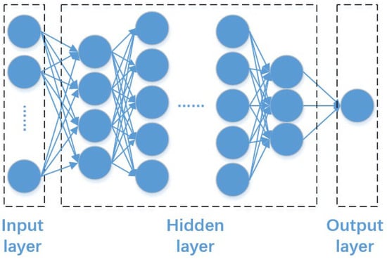
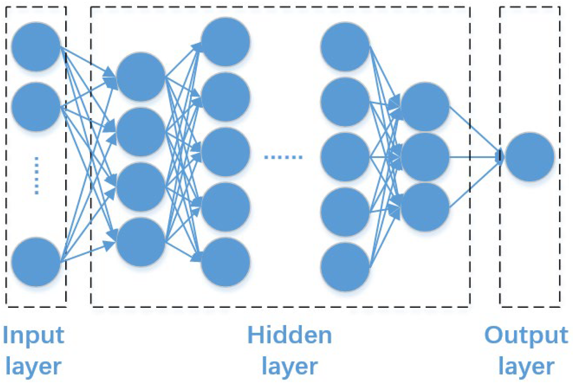
Figure 3. Schematic diagram of MLP.

Hochreiter proposed the LSTM structure in 1997. The LSTM uses three gate control units including forgetting gate Z^f, input gate Zⁱ and output gate Z^o to control the memory level of history information in the hidden layer so as to retain the necessary information and forget unimportant information [27]. The Sigmoid function is used to represent the on-off-state of the gate, as shown in Equation (1).

$$\mathrm{Sigmoid}: \sigma \left(\mathrm{x}\right)={\displaystyle \frac{1}{1+{\mathrm{e}}^{-\mathrm{x}}}}$$

(1)

The “memory-forgetting” functionality in LSTM is achieved through complex gating mechanisms, which introduce a substantial number of trainable parameters, thereby increasing model complexity and training difficulty. Noting this limitation, Cho et al. observed a key correlation: the retention of historical information is intrinsically linked to the forgetting rate. In essence, a stronger memory of past information corresponds to less forgetting. This insight—that memory and forgetting are two sides of the same coin—inspired the design of a more streamlined architecture. Therefore, the forgetting gate Z^f and input gate Zⁱ in LSTM can be combined into one gated unit. On this basis, the GRU model was proposed in 2014, and its principle is shown in Figure 2. Two units, the update gate z and the reset gate r, are used to control the information, whose performance is similar to that of LSTM and involves fewer parameters [28].

Therefore, parameter prediction based on the GRU model is carried out in this paper. The value of the updated gate z and the reset gate r of GRU model is shown in Formulas (2) and (3).

$$\mathrm{r}=\sigma \left({\mathrm{W}}^{\mathrm{r}}\left({\displaystyle \frac{{\mathrm{x}}^{\mathrm{t}}}{{\mathrm{h}}^{\mathrm{t}-1}}}\right)\right)$$

(2)

$$\mathrm{z}=\sigma \left({\mathrm{W}}^{\mathrm{z}}\left({\displaystyle \frac{{\mathrm{x}}^{\mathrm{t}}}{{\mathrm{h}}^{\mathrm{t}-1}}}\right)\right)$$

(3)

where W^r is the weight matrix of update gate r, and W^z is the weight matrix of reset gate z. $\left({\displaystyle \frac{{\mathrm{x}}^{\mathrm{t}}}{{\mathrm{h}}^{\mathrm{t}-1}}}\right)$ is the combination matrix of input vector ${\mathrm{x}}^{\mathrm{t}}$ and hidden state vector ${\mathrm{h}}^{\mathrm{t}-1}$.

The function of the reset gate R is to extract the short-term memory information contained in the history information. The function of the update gate Z is to update the information of the new moment to the history information. The calculation methods of the parameters in GRU model are listed as follows:

(1)

${\mathrm{h}}^{\mathrm{t}-1^{\prime }}$ represents the short-term memory content extracted by the history information ${\mathrm{h}}^{\mathrm{t}-1}$ after the reset gate R processing, as shown in Equation (4).

$${\mathrm{h}}^{\mathrm{t}-1^{\prime }}={\mathrm{h}}^{\mathrm{t}-1}\odot \mathrm{r}$$

(4)

(2)

${\mathrm{h}}^{\prime }$ represents the current moment information formed by integrating the short-term memory ${\mathrm{h}}^{\mathrm{t}-1^{\prime }}$ and the external input information of the current moment ${\mathrm{x}}^{\mathrm{t}}$, as shown in Equation (5).

$${\mathrm{h}}^{\prime }=\tan \mathrm{h}\left(\mathrm{W}\left({\displaystyle \frac{{\mathrm{x}}^{\mathrm{t}}}{{\mathrm{h}}^{\mathrm{t}-1}}}\right)\right)$$

(5)

(3)

${\mathrm{h}}_{\mathrm{t}}$ represents the long-term memory information transferred from the current moment to the next moment, as shown in Equation (6), which is formed by the fusion of the retained part of the long-term memory information ${\mathrm{h}}^{\mathrm{t}-1}$ of the previous moment and the short-term memory information ${\mathrm{h}}^{\prime }$ of the current moment. According to the definition of updated gate z, the corresponding coefficients are (1 − z) and z, respectively. $\left(1 - \mathrm{z}\right)\odot {\mathrm{h}}^{\mathrm{t}-1}$ indicates that the current moment selectively forgets the information remembered at the last moment, and $\mathrm{z}\odot {\mathrm{h}}^{\prime }$ indicates that the current moment selectively remembers the information. The sum of the two is the hidden information ${\mathrm{h}}_{\mathrm{t}}$ transmitted from the current moment to the next moment. GRU describes memory by using the value of the updated gate z, which is the result of Sigmoid function with z∈(0,1). (1 − z) represents forgetting, and 1 − z∈(0,1), thus realizing the combination of “memory-forgetting” steps.

$${\mathrm{h}}^{\mathrm{t}}=\left(1 -\mathrm{z}\right)\odot {\mathrm{h}}^{\mathrm{t}-1}+\mathrm{z}\odot {\mathrm{h}}^{\prime }$$

(6)

(4)

${\mathrm{y}}^{\mathrm{t}}$ represents the final output of GRU unit, as shown in Equation (7).

$${\mathrm{y}}^{\mathrm{t}}=\sigma \left({\mathrm{W}}^{\mathrm{o}}\left({\displaystyle \frac{{\mathrm{x}}^{\mathrm{t}}}{{\mathrm{h}}^{\mathrm{t}-1}}}\right)+{ \mathrm{b}}^0\right)$$

(7)

where $\left({\displaystyle \frac{{\mathrm{x}}^{\mathrm{t}}}{{\mathrm{h}}^{\mathrm{t}-1}}}\right)$ is the splicing matrix of input vector ${\mathrm{x}}^{\mathrm{t}}$ and hidden state vector ${\mathrm{h}}^{\mathrm{t}-1}$.

2.2. Principle of the Anomaly Detection Stage

While RNNs are effective for time-series prediction, their structure is suboptimal for direct anomaly detection [29]. Compounding this issue, the fixed thresholds typically used in “prediction-detection” schemes often lead to false alarms. This work proposes the integration of an MLP model to mitigate these shortcomings and achieve precise anomaly detection in NPP operational data.

The Multilayer Perceptron (MLP) is a fundamental type of feedforward artificial neural network. Its architecture, as illustrated in Figure 3, consists of an input layer, one or more hidden layers, and an output layer. This structure enables the MLP to perform non-linear classification and function approximation, mapping an N-dimensional input vector to a desired output space.

An MLP accepts a feature vector as input, which is then transformed through one or more hidden layers. The model must contain at least one hidden layer, and each layer can comprise an arbitrary number of neurons (nodes). Generally, increasing the number of neurons and hidden layers enhances the model’s capacity for nonlinear approximation, allowing it to learn more complex representations. An MLP is a fully connected network where all neurons in one layer connect to all neurons in the adjacent layers, forming a complete bipartite graph between layers. It features no intra-layer connections and employs a simple, unprocessed feedforward design. The structure is simple, and the training effect is only positively correlated with the number of nodes and hidden layers. ${\mathrm{Out}}_{\mathrm{i}}$ is calculated with Equation (8):

$${\mathrm{Out}}_{\mathrm{i}} = {{\mathrm{f}}_{\mathrm{i}}(\mathrm{W}}_{\mathrm{i}}\odot {\mathrm{a}}_{\mathrm{i}} +{ \mathrm{b}}_{\mathrm{i}})$$

(8)

where ${\mathrm{a}}_{\mathrm{i}}={\mathrm{Out}}_{\mathrm{i}-1}$. ${\mathrm{f}}_i$ represents the activation function. The commonly used activation functions include Sigmoid, tanh, ReLU, and Softmax.

An MLP is built from layers of simple neurons, where each neuron is connected to all neurons in the adjacent layers. The network approximates complex non-linear functions from inputs to outputs through the aggregated processing of these neurons. This structure enables potent learning and adaptive capabilities via training algorithms like backpropagation.

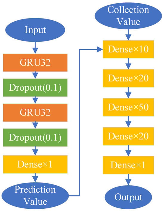
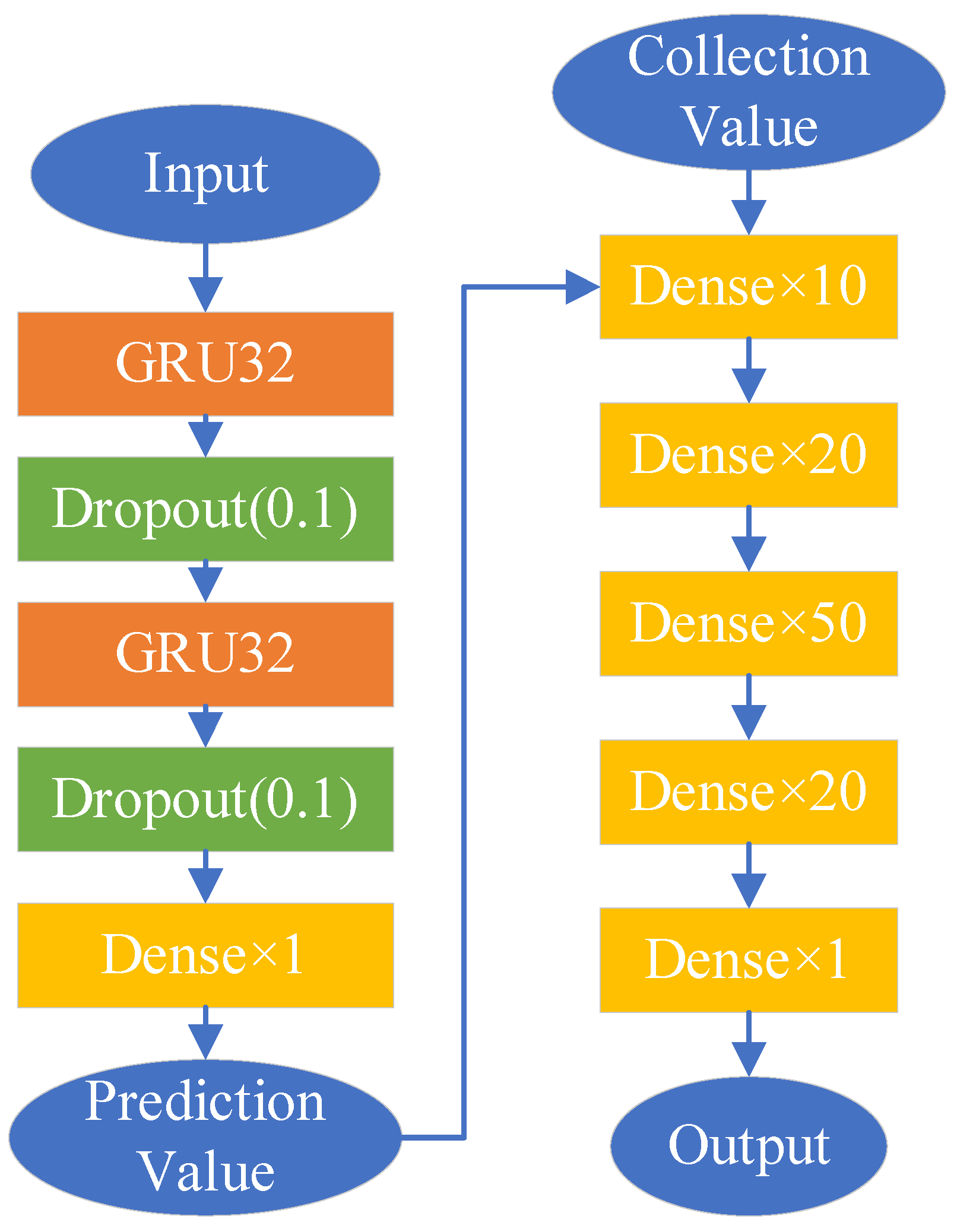
According to the above design, the GRU-MLP model is designed, and its structure is shown in Figure 4.

Figure 4. Structural diagram of GRU-MLP.

3. Algorithm Design for Anomaly Detection and Correction of NPP

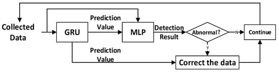
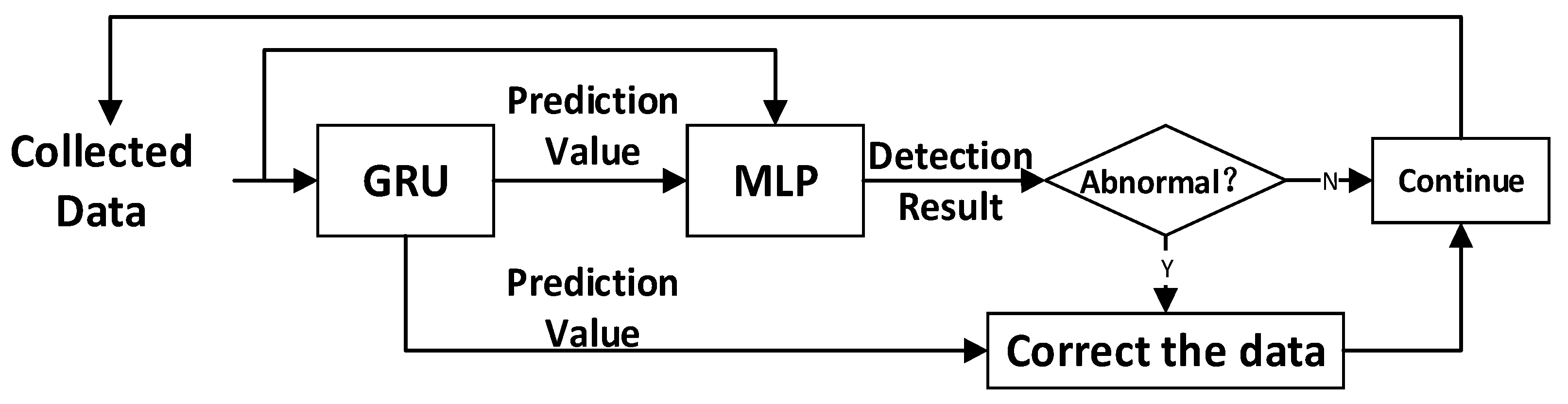
Based on the aforementioned principles, this work presents an integrated algorithm for the detection and correction of anomalies in NPP operational data. The overall architecture of the proposed algorithm is illustrated in Figure 5. The procedure involves three key stages: first, a GRU model predicts the parameter values; second, an MLP model compares the collected values against the corresponding predictions to determine anomalies; finally, identified anomalies are rectified by replacing them with the predicted values.

Figure 5. Algorithm strategy diagram.

The model training and application methods for the prediction stage are as follows: Assume that an operation parameter of NPP is a(t). Its data sampling period is τ, and a data time window of length l slides forwards in time. Let the starting point of the window be t = t0, and the ending point be t = t0 + (l − 1)τ. Input the data a(t0)~a(t0 + (l − 1)τ) into the GRU model and mark a(t0 + lτ) as the conclusion for training. The time window slides forward by one unit of time τ at each step, and training proceeds iteratively until the model converges according to the predefined criteria. Upon completion of training, a dedicated GRU model is obtained for each parameter. During the inference phase, an input sequence of length l is fed into the corresponding model to generate the prediction result.

The model training and application methods for the detection stage are as follows: Assume that an operation parameter of NPP is b(t). To train the MLP model for anomaly detection to the b(t), a series of input is required, including the prediction value of the NPP parameter b at t = t1, b(t1), the collected value of parameter b at t1, b (t1)′ and the conclusions marked with 0 or 1 depending on whether the data anomalies exist. Among them, b(t1) is calculated by inputting data b(t1 − lτ)~b(t1 − 1τ) into the GRU model. The MLP model is trained to identify the difference between b(t1) and b (t1)′ and shifted by comparing with the marked conclusion.

Leveraging the anomaly detection results, the identified outliers in the collected data are replaced with the corresponding predictions from the GRU model, thereby rectifying anomalies in the NPP operational data.

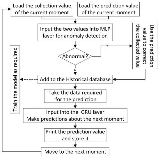
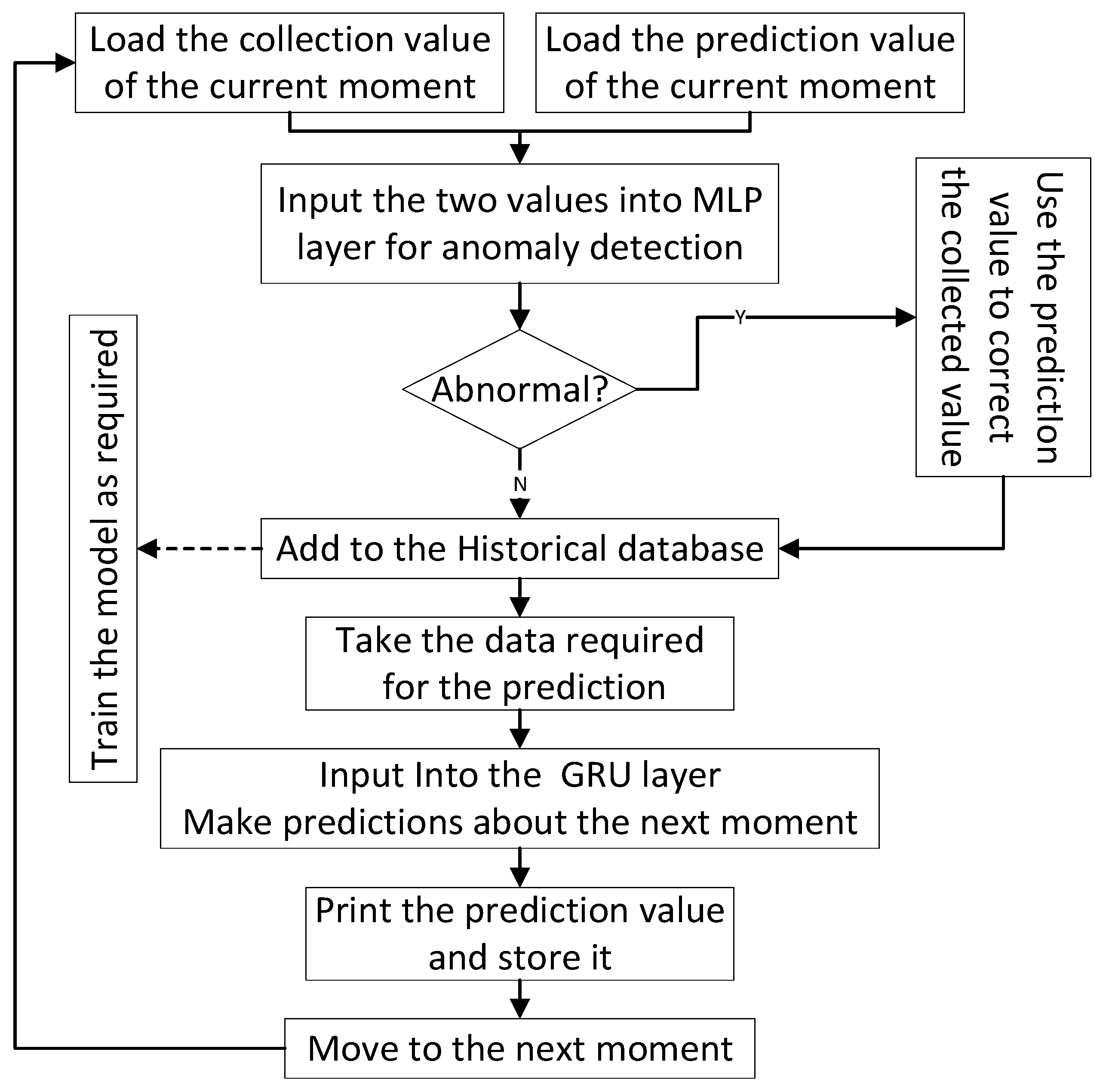
The algorithm flow is shown in Figure 6.

Figure 6. Algorithm flow diagram.

4. Parameter Prediction Performance Verification

4.1. Design of the Parameter Prediction Experiments

A set of operation data of a NPP with pressurized water reactor (PWR) is used as the experimental data set. Several experiments are carried out to verify the prediction performance of the designed algorithm. In order to facilitate observation and comparison, the operation data of the NPP are normalized. The normalization formula is shown in Equation (9):

$$\mathrm{Y} = {\displaystyle \frac{\mathrm{X} - \mathrm{b}}{\mathrm{a} - \mathrm{b}}}$$

(9)

where X represents the original data and Y represents the normalized data, a and b are the scaling coefficient and bias coefficient, respectively. Let the data set selected by an experiment be N; then, a is the maximum value of N and b is the minimum value of N.

The collected pressure data from the pressurizer (PZR) served as the experimental data set. It was partitioned into a training set (the first 80%) and a test set (the remaining 20%). In this experiment, prediction horizons were set to 1, 3, 5, 10, and 20 steps. By forecasting data across these varying horizons, the model’s performance was evaluated to validate the efficacy and applicability of the GRU model for predicting NPP operational data.

4.2. Experimental Results

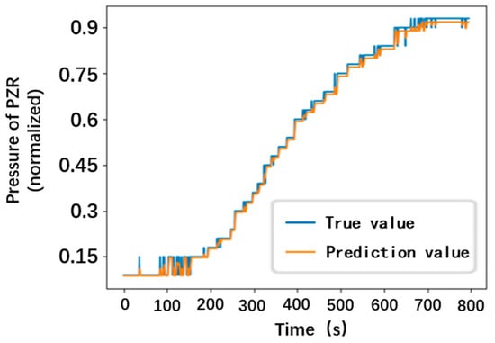
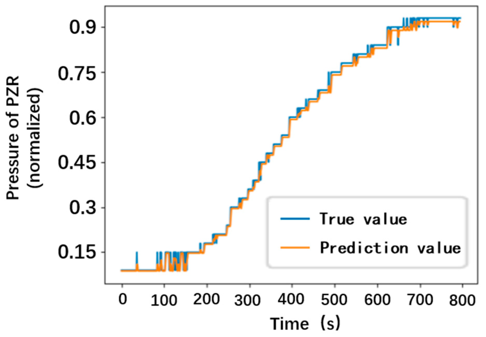
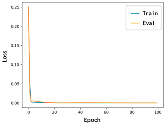
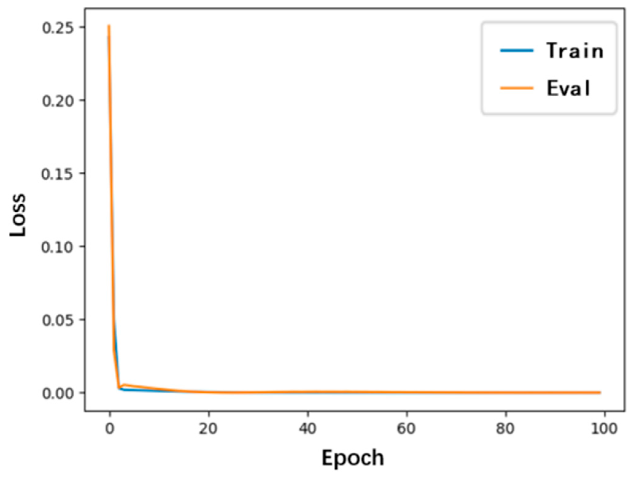
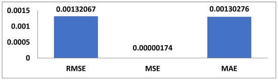
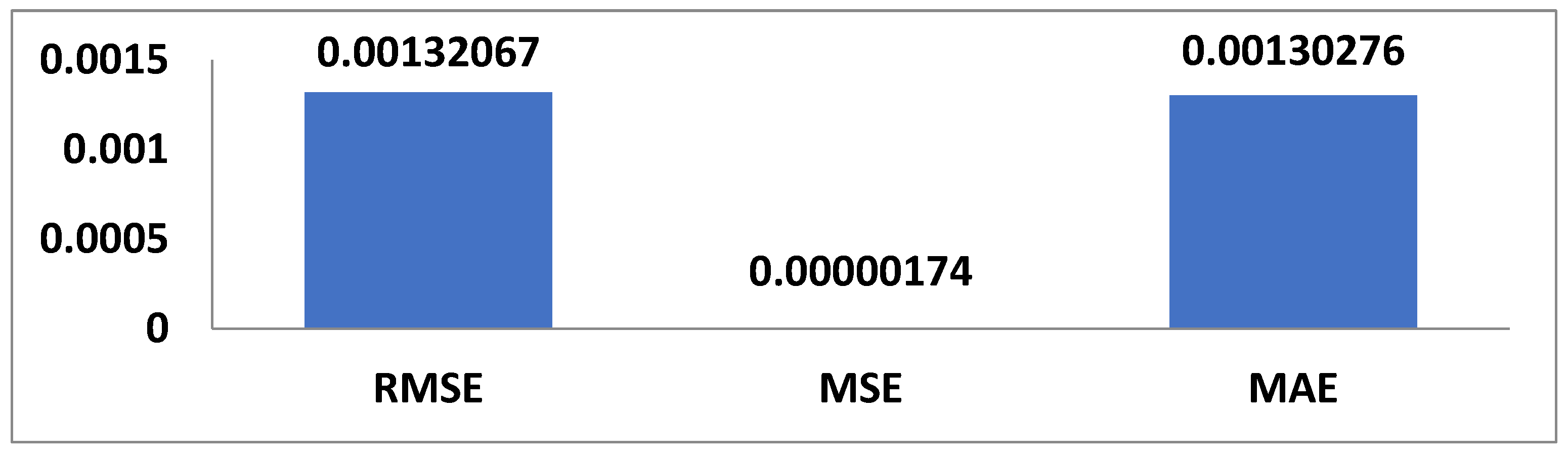
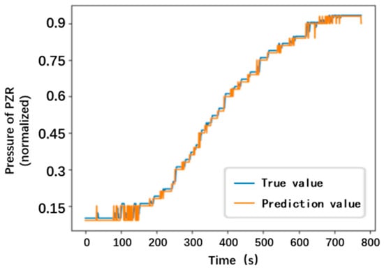
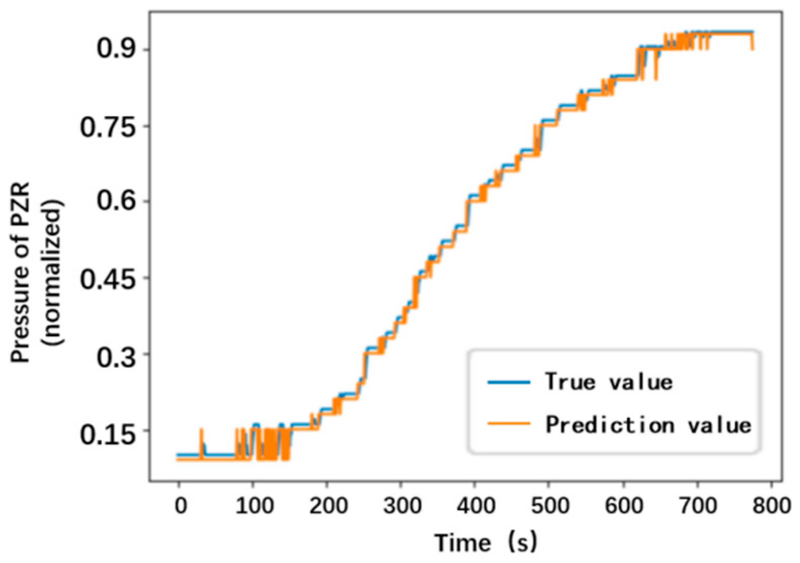
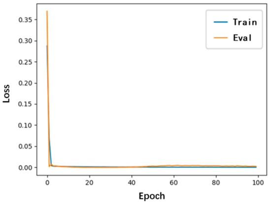
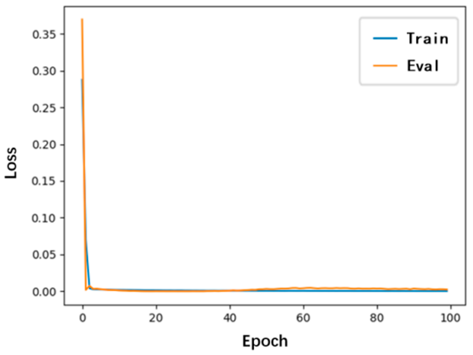
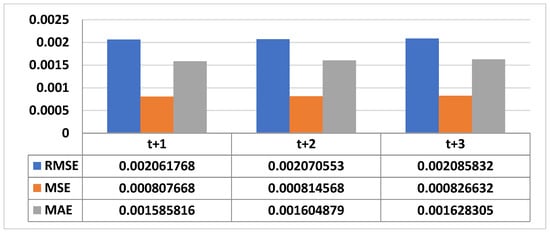
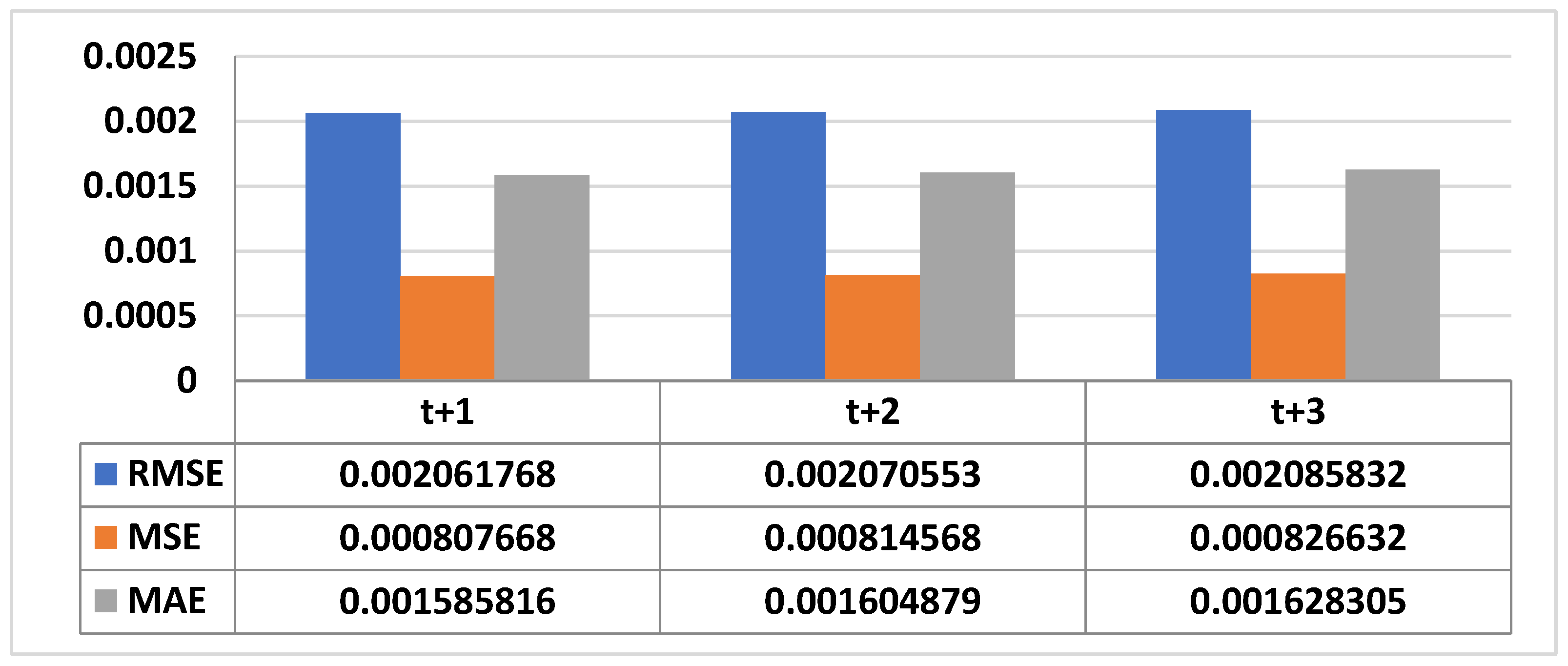
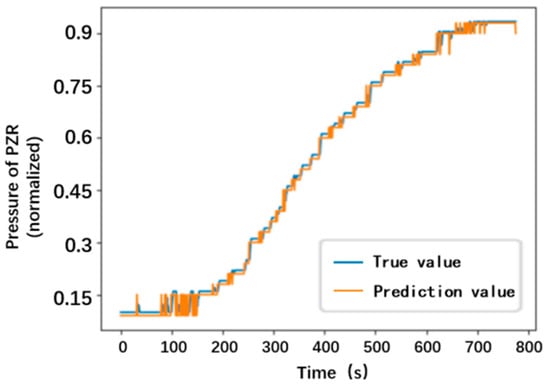
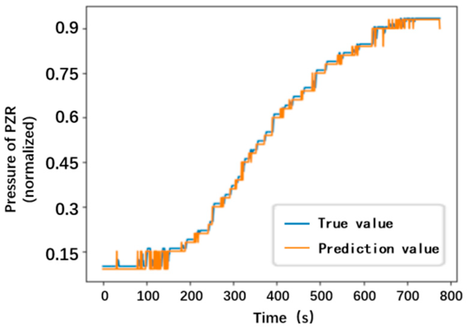
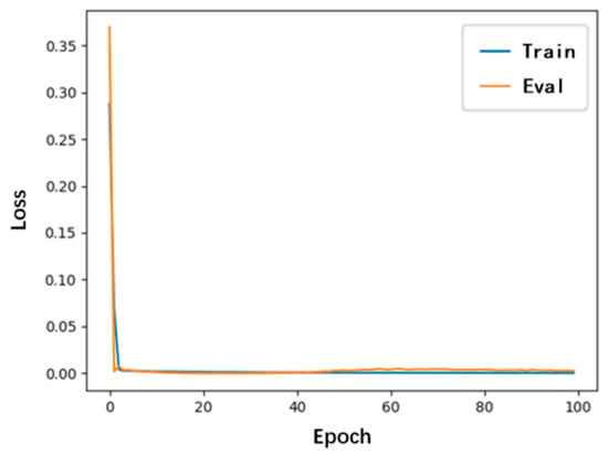
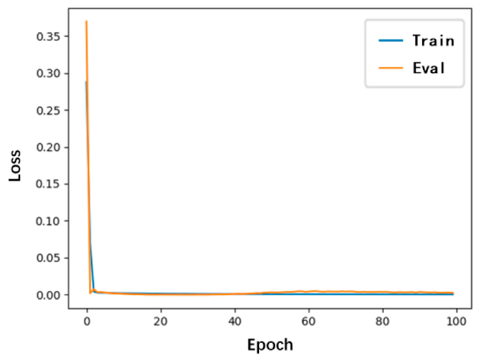
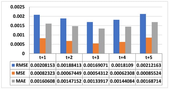
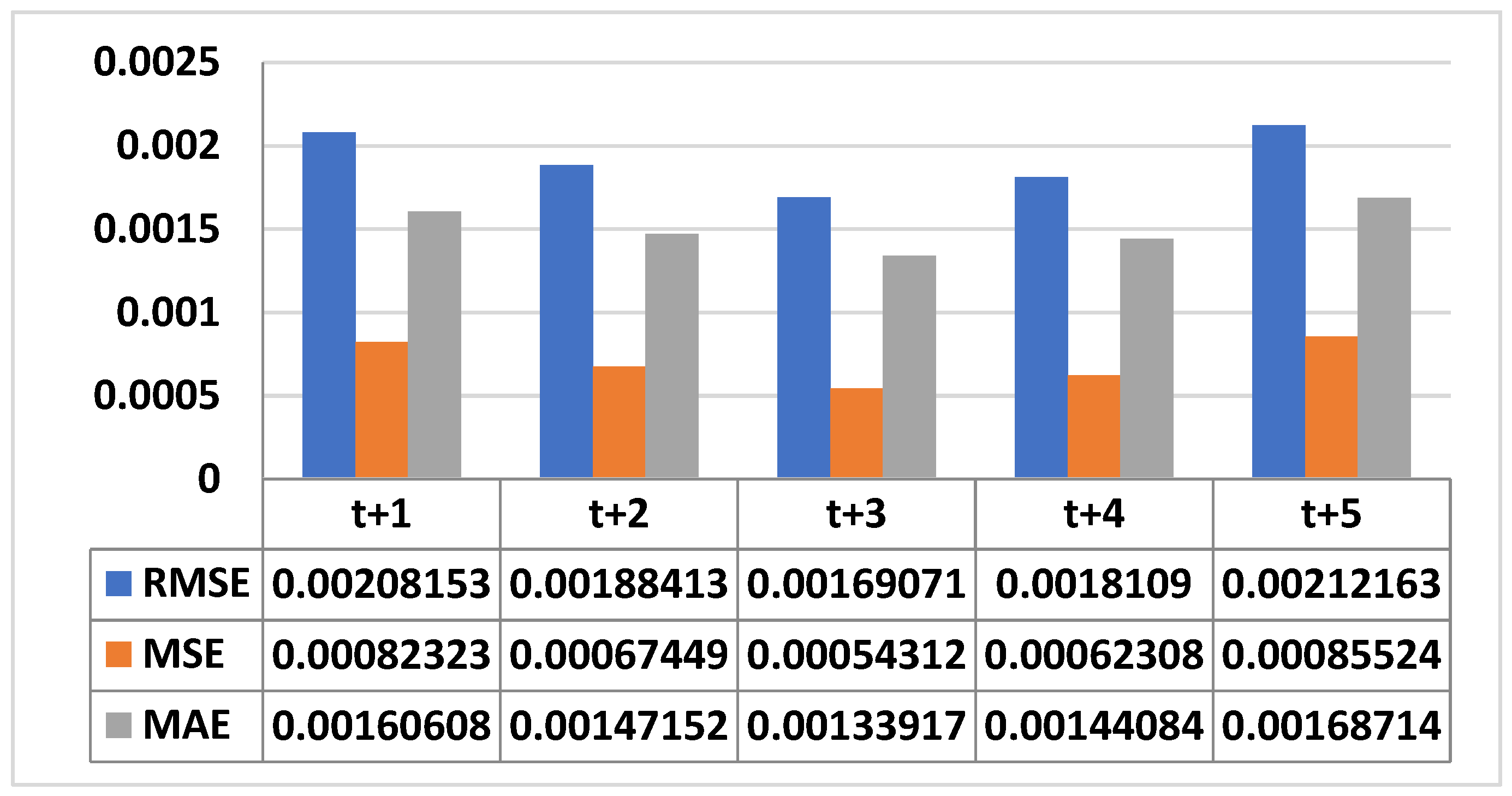
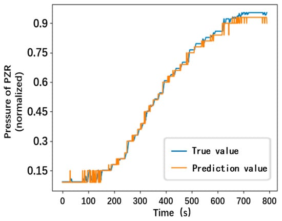
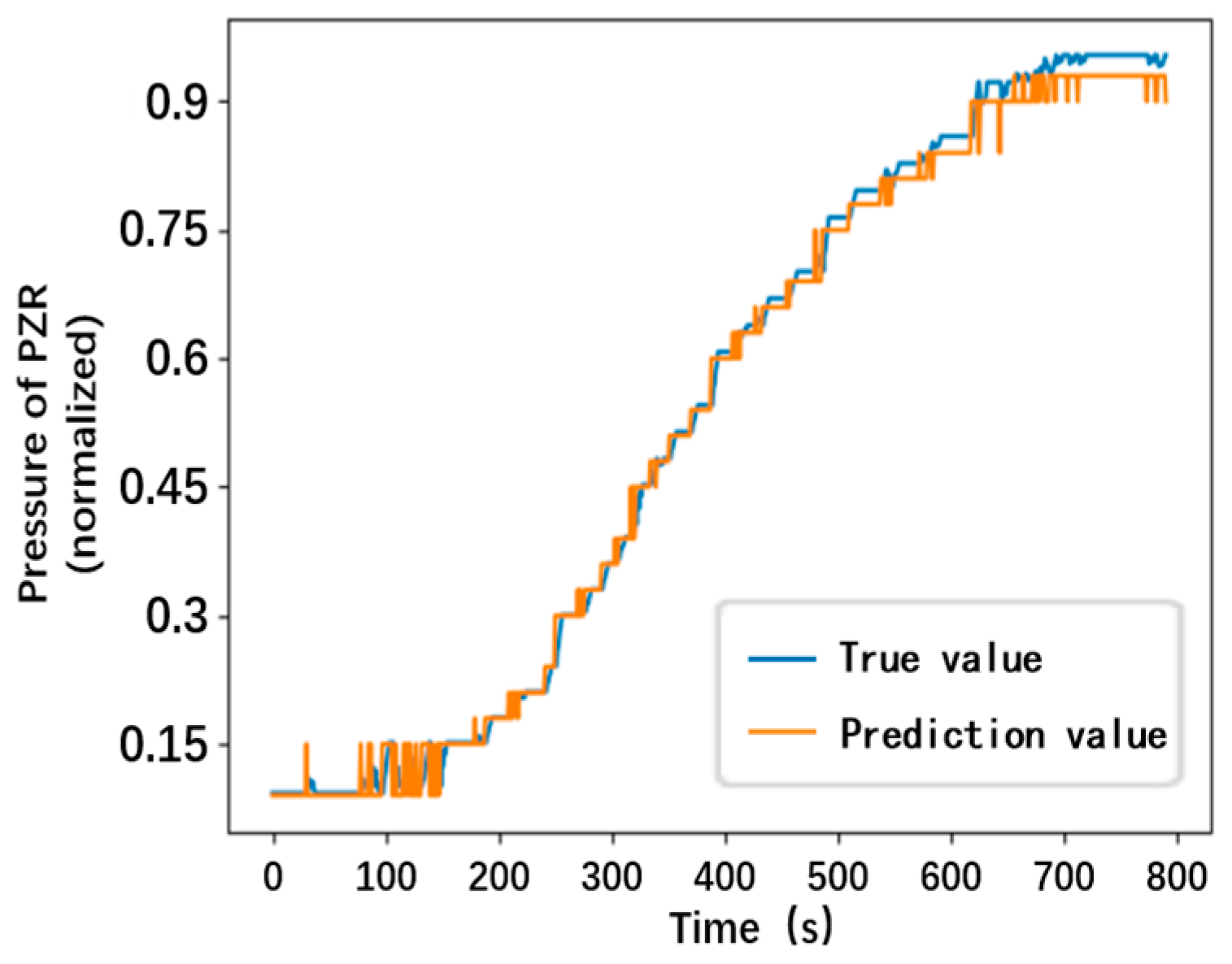
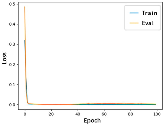
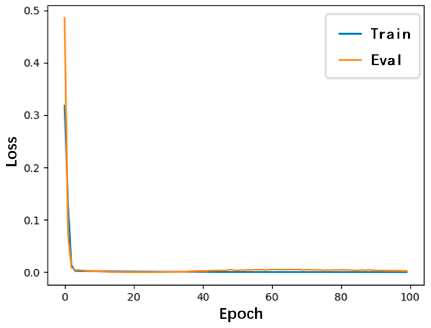
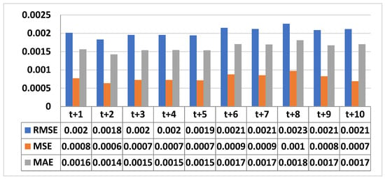
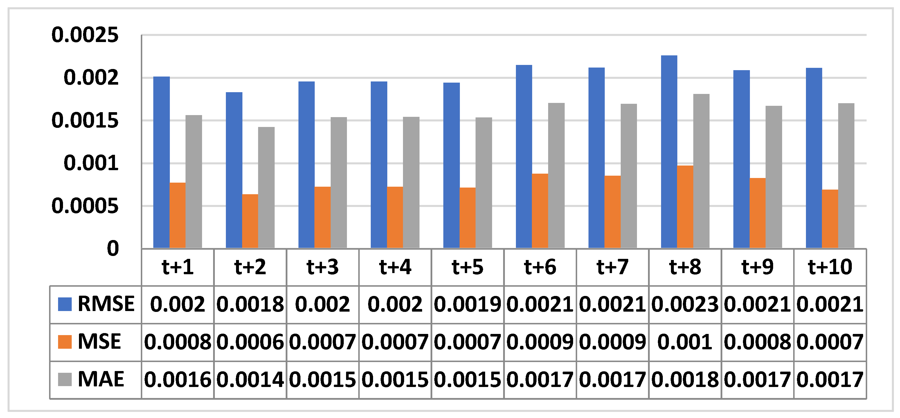
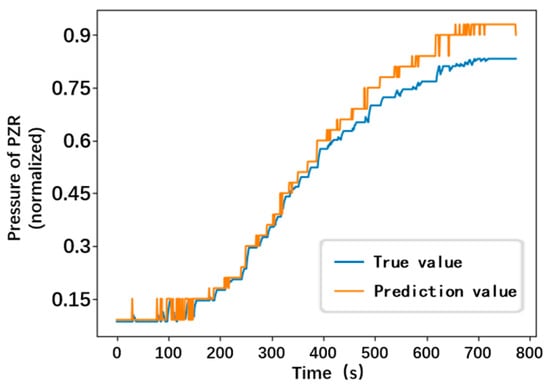
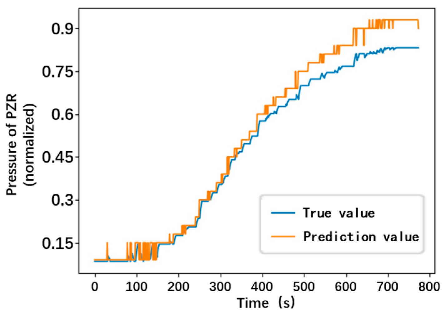
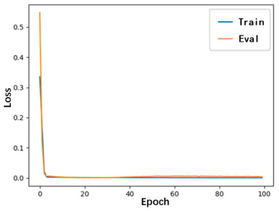
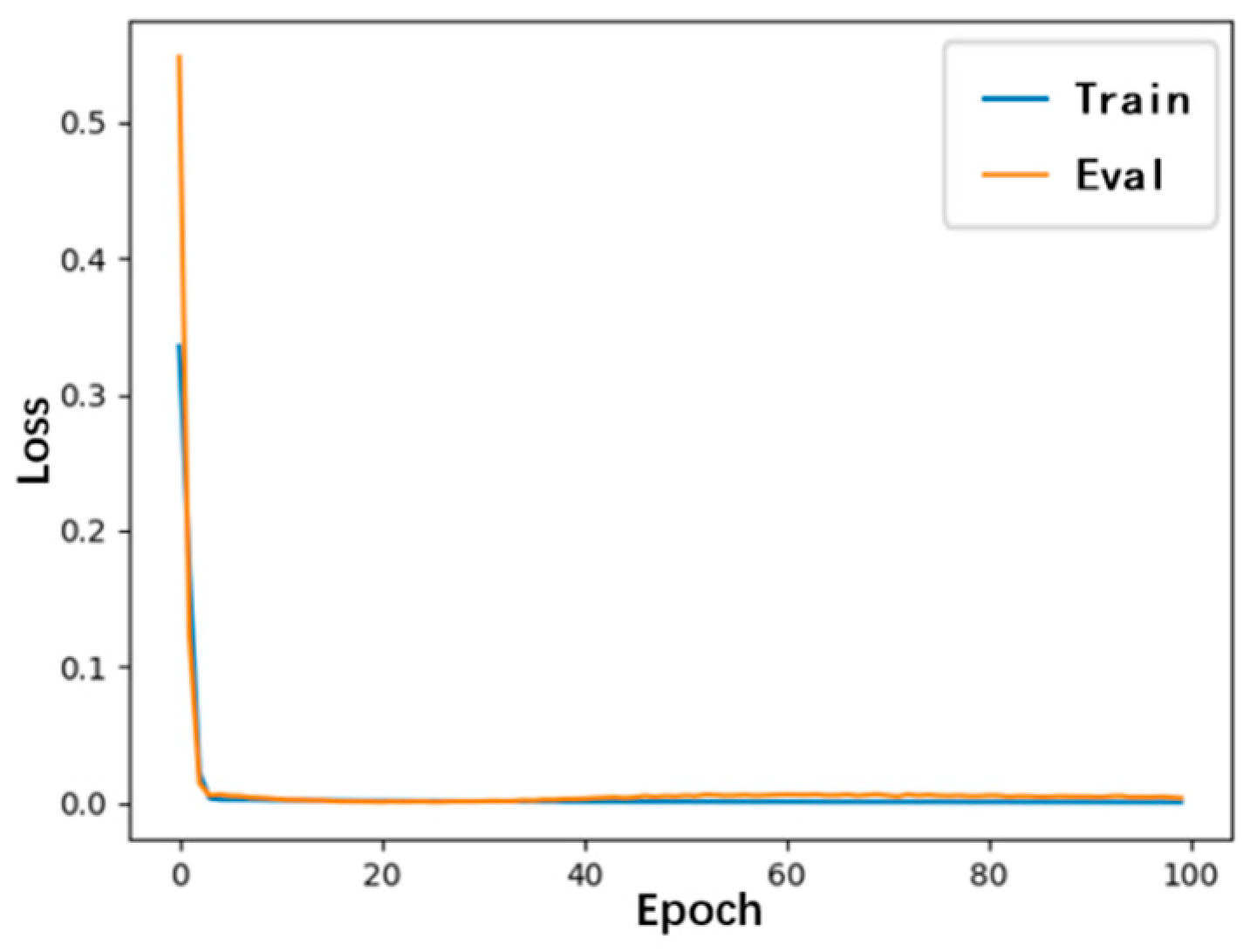
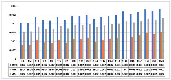
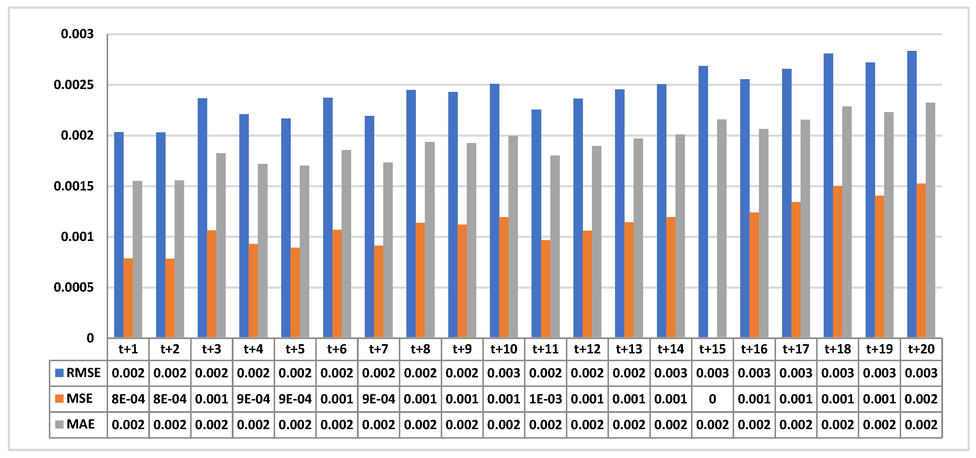
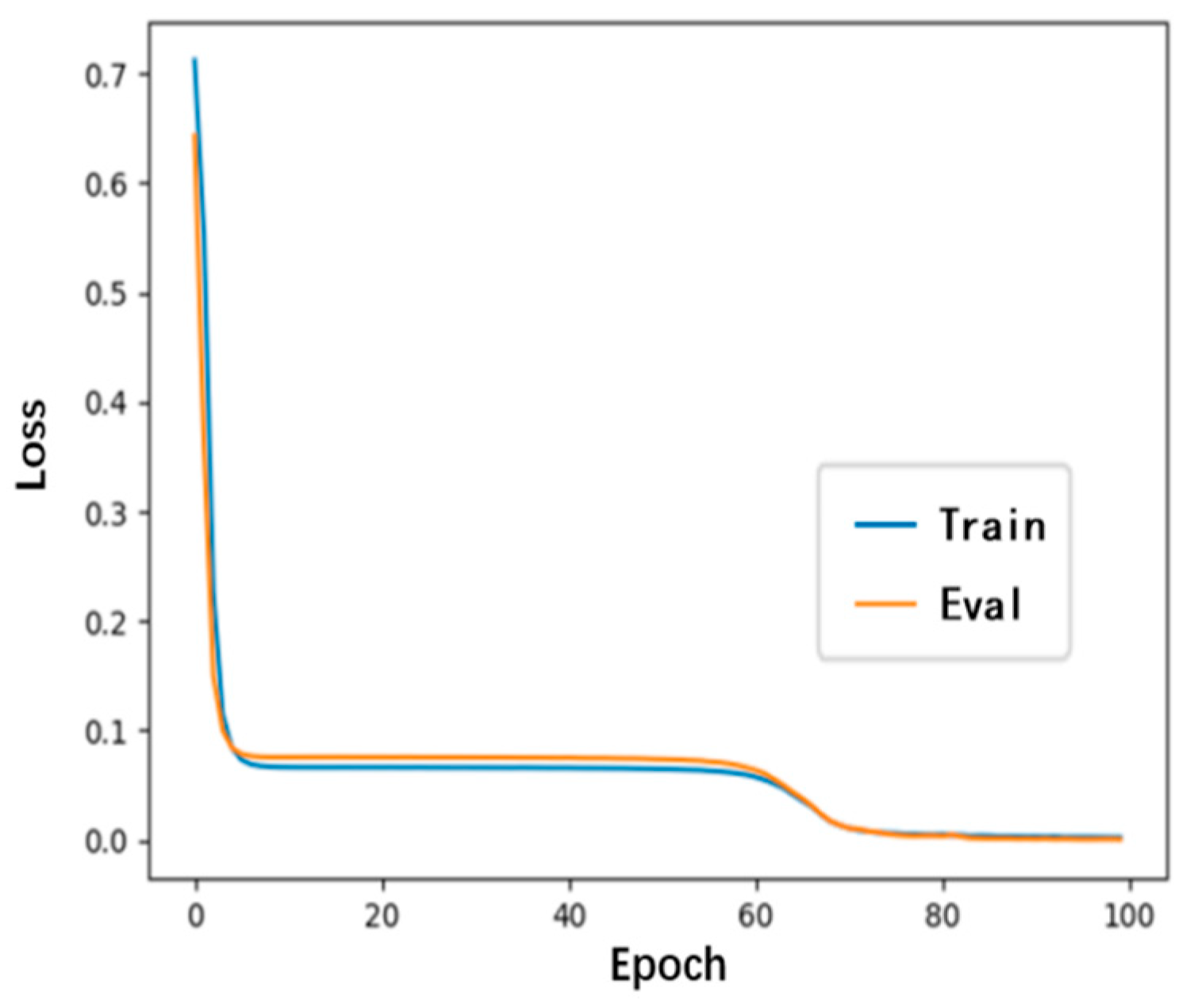
The performance of the GRU model for NPP operational data was evaluated from multiple perspectives, with the experimental results visualized using three types of figures. A prediction performance plot, which compares predicted values against actual values, serves to visually assess the model’s accuracy. The convergence behavior of the GRU model during training is demonstrated by the loss curve, which illustrates the training feasibility and efficiency. For quantitative evaluation, three metrics were employed: Root Mean Square Error (RMSE), Mean Square Error (MSE), and Mean Absolute Error (MAE). These metrics comprehensively assess the prediction accuracy from different aspects. A summary of the experimental results and their corresponding figures is provided in Table 1, with the detailed results presented in Figure 7, Figure 8, Figure 9, Figure 10, Figure 11, Figure 12, Figure 13, Figure 14, Figure 15, Figure 16, Figure 17, Figure 18, Figure 19, Figure 20 and Figure 21.

Table 1. Results of the parameter prediction experiments.

Experiment Number	Prediction Step	Experimental Results
		Prediction Effect	Loss Curve	Error Indexes
1	1 step	Figure 7	Figure 8	Figure 9
2	3 steps	Figure 10	Figure 11	Figure 12
3	5 steps	Figure 13	Figure 14	Figure 15
4	10 steps	Figure 16	Figure 17	Figure 18
5	20 steps	Figure 19	Figure 20	Figure 21

Figure 7. One-step prediction effect.

Figure 8. Loss curve for 1-step prediction.

Figure 9. Diagram of 1-step prediction error indexes.

Figure 10. Three-step prediction effect.

Figure 11. Loss curve for 3-step prediction.

Figure 12. Diagram of 3-step prediction error indexes.

Figure 13. Five-step prediction effect.

Figure 14. Loss curve for 5-step prediction.

Figure 15. Diagram of 5-step prediction error indexes.

Figure 16. Ten-step prediction effect.

Figure 17. Loss curve for 10-step prediction.

Figure 18. Schematic diagram of 10-step prediction error index.

Figure 19. Twenty-step prediction effect.

Figure 20. Loss curve for 20-step prediction.

Figure 21. Diagram of 20-step prediction error indexes.

4.3. The Conclusion of the Prediction Experiments

The following conclusions can be drawn from the comparative analysis of the experimental results from Experiment 1 to Experiment 5 (influence and effect of step size prediction):

(1)

In the process of prediction and testing, the loss of GRU model converge very fast (within 20 epochs), and eventually all stabilize near 0, showing a good application effect and high efficiency.

(2)

With the increase in the prediction step, the initial loss value of GRU model increases. The differences between the prediction value and the true value increase slightly, and the value of three error indexes increase at the same time, indicating that the increasing of the step size will lead to the increasing of prediction difficulty.

(3)

By comparing the value of the three error indexes for different prediction steps in the same experiment, it can be concluded that the later the prediction step in the same time window is, the larger error with the real value will be.

(4)

For all kinds of predicted step sizes, the final training and testing errors of GRU model are small and the accuracy is high.

5. Anomaly Detection Performance Verification

5.1. Design of the Anomaly Detection Experiments

This section aims to validate the accuracy and efficiency of the proposed GRU-MLP algorithm through experimental evaluation. The algorithm’s accuracy is quantified by its performance in correctly identifying the operational state of the data. The efficiency of the algorithm is assessed by the convergence rate of the loss function during the training and testing of the GRU-MLP model. To comprehensively validate the algorithm’s capability in identifying various data anomalies in NPPs, the experiments in this section encompass all typical types of data acquisition anomalies that frequently occur in operational scenarios. The experiments encompass the detection of three primary anomaly types: random jump, fixed drift, and growth drift. The growth drift category is further subcategorized into its most representative forms: linear, polynomial, and logarithmic growth. Taking the simulating operation data of a NPP with PWR as the experimental data set, the designed experiments are carried out. Details of the experiments are shown in Table 2.

Table 2. Details of the anomaly detection experiments.

Experiment Number		Anomaly Style		Parameter	Length	Start Time	Growth Style
1		Random jump		Pressure of PZR	7000	100 random points	-
2		Fixed-value drift		Water level of PZR	5000	2500	-
3	(a)	Growth drift	Linear growth	Pressure of PZR	5000	2500	Δy = a(t − 2500) + δ
	(b)		Polynomial growth	Average temperature of primary loop	5000	2500	Δy = b(t − 2500)2 + δ
	(c)		Logarithmic growth	Pressure of PZR	3000	1800	Δy = c × n (t − 1800) + δ

5.2. Results of the Experiments

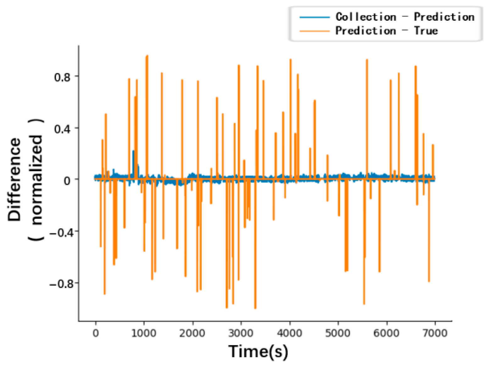
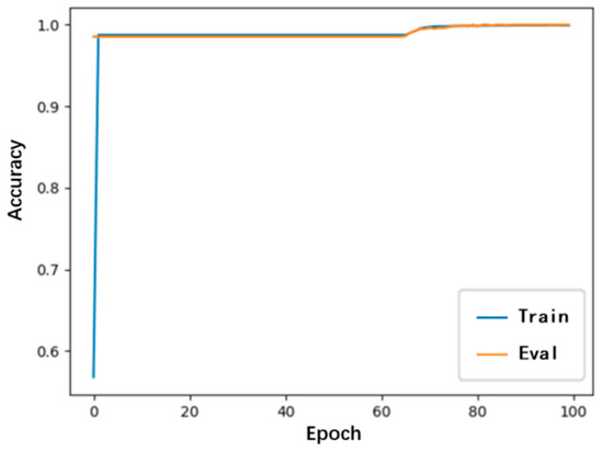
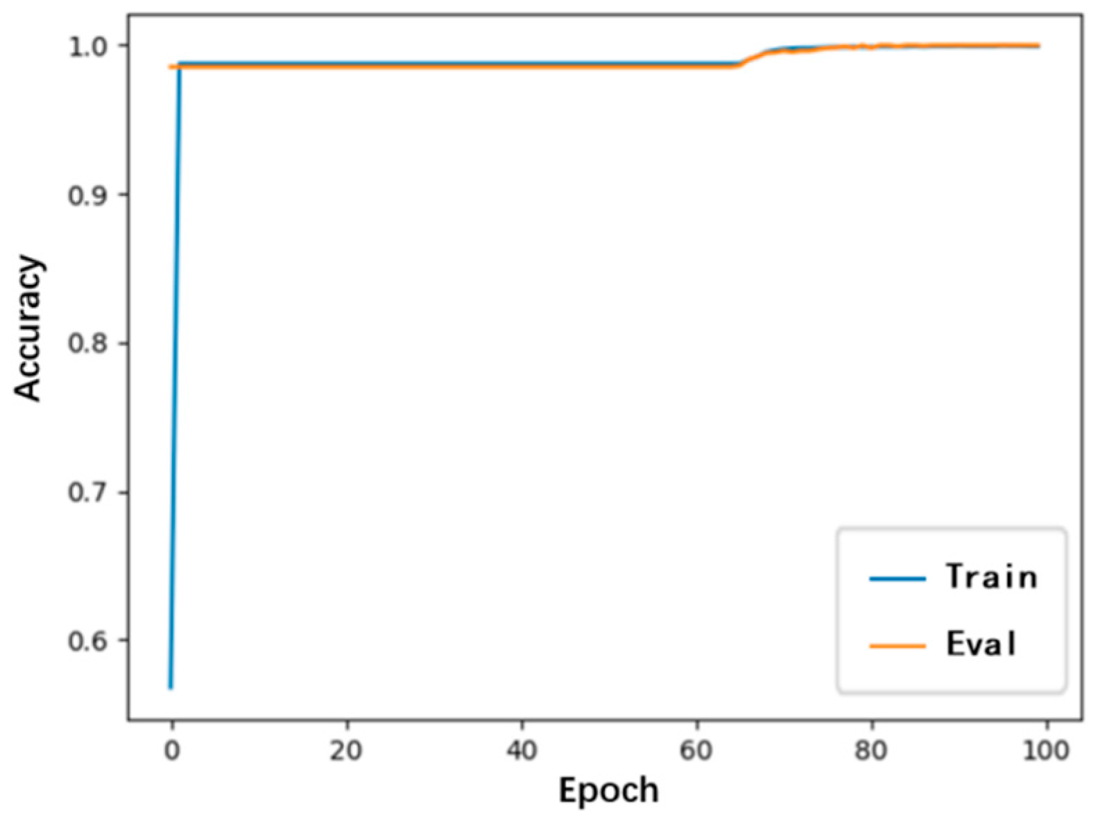
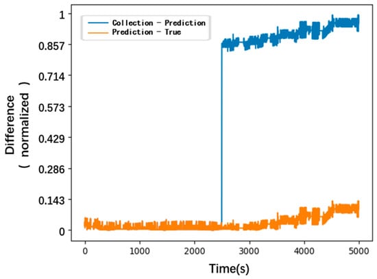
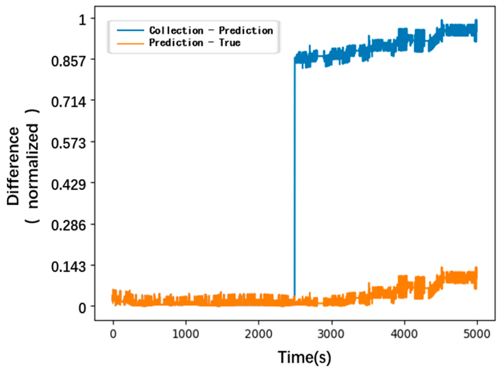
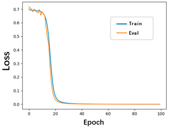
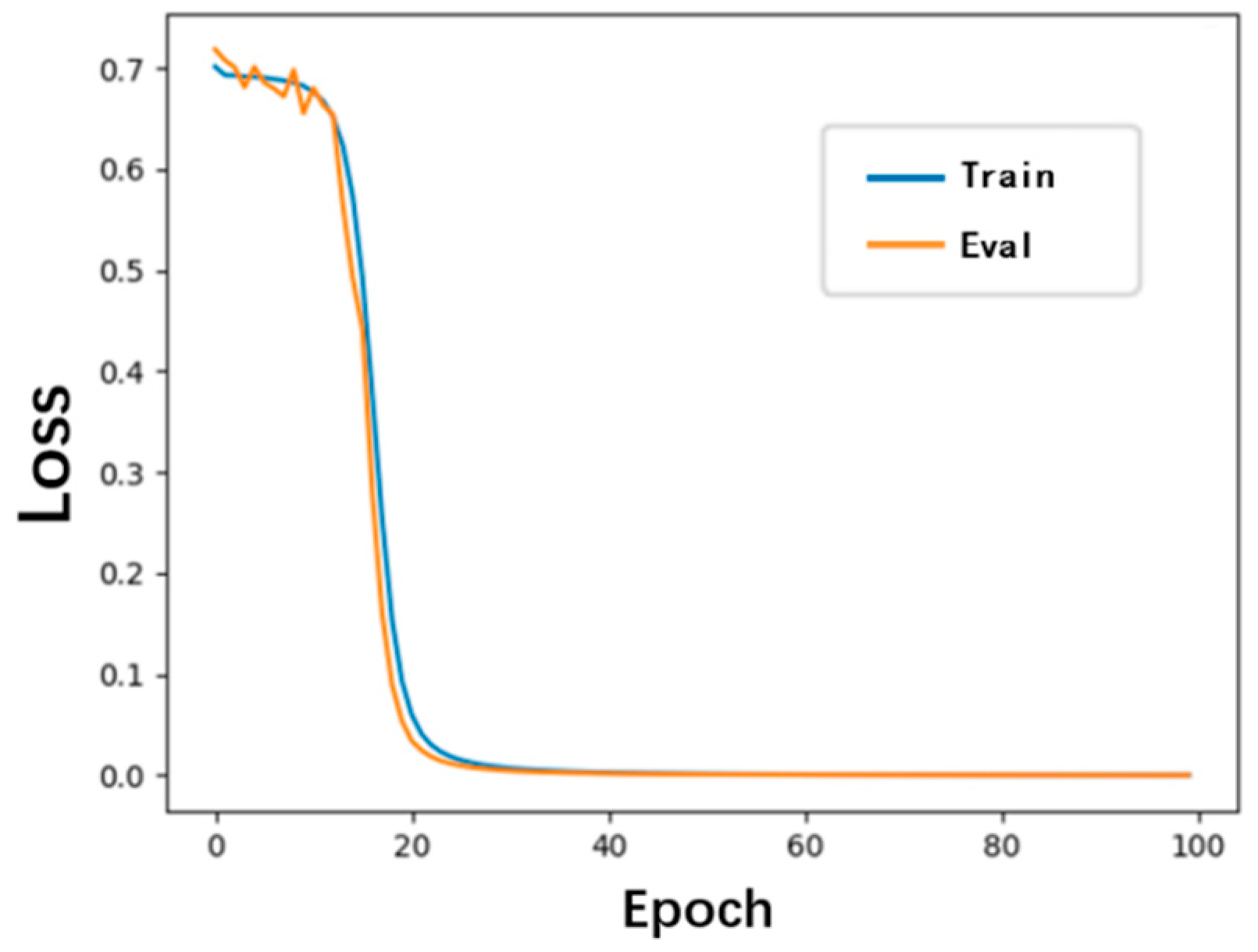
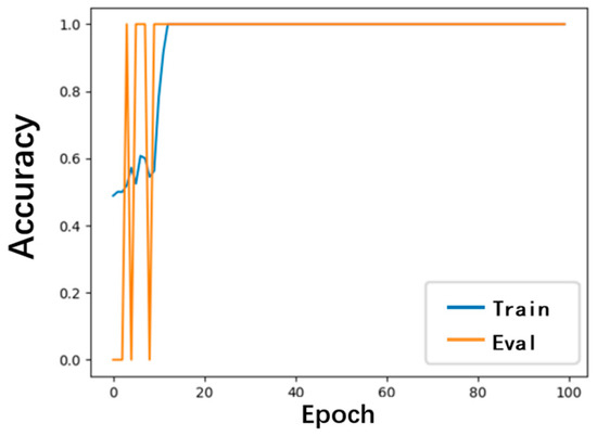
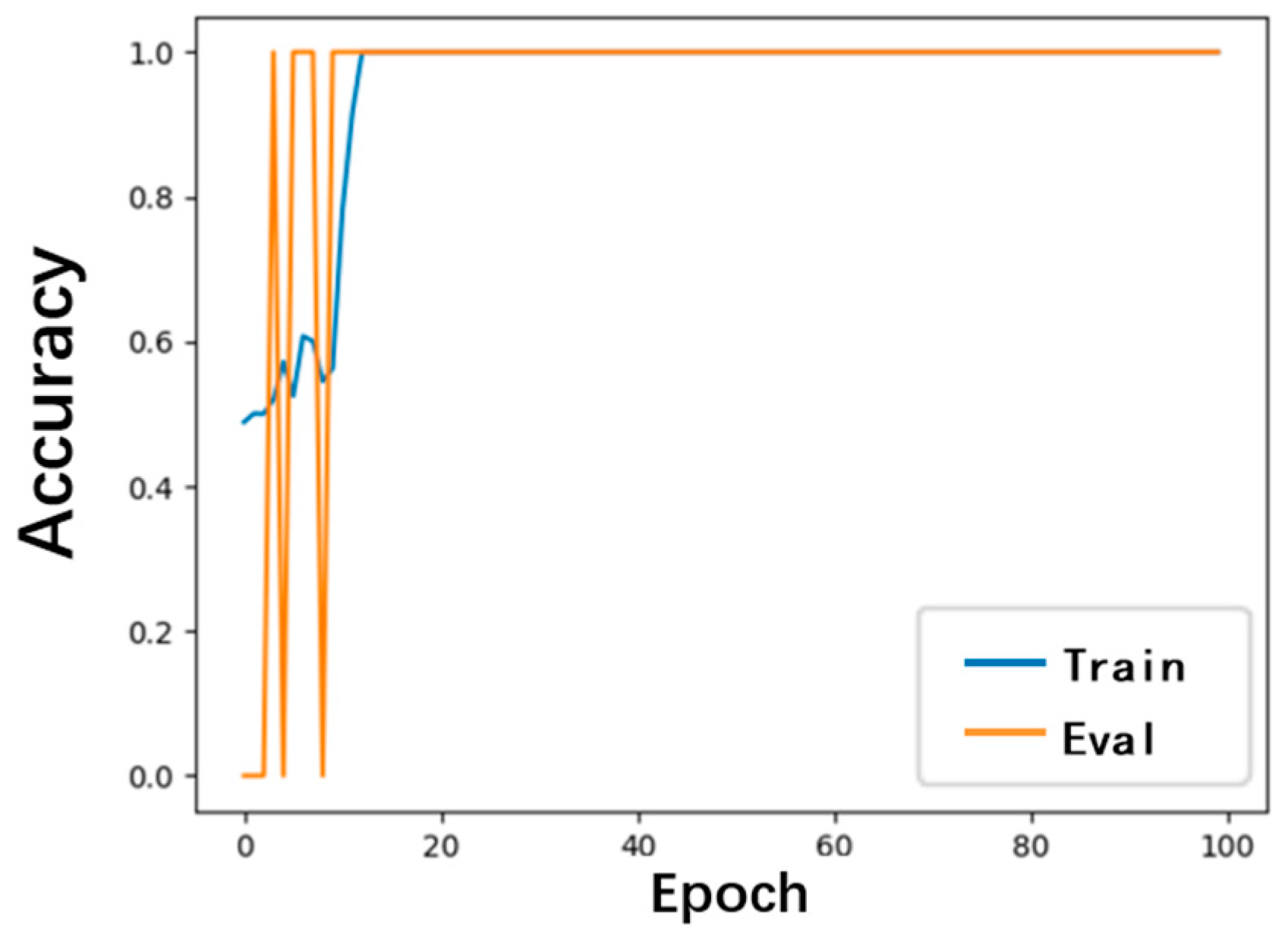
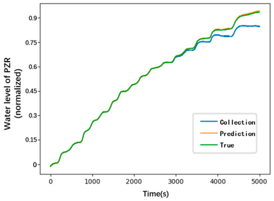
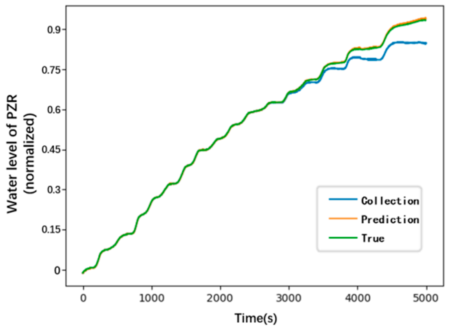
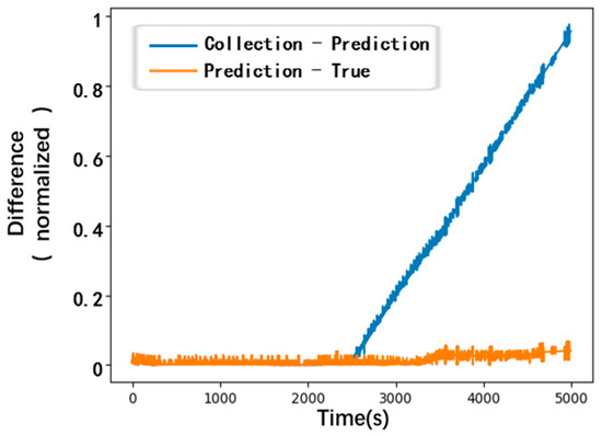
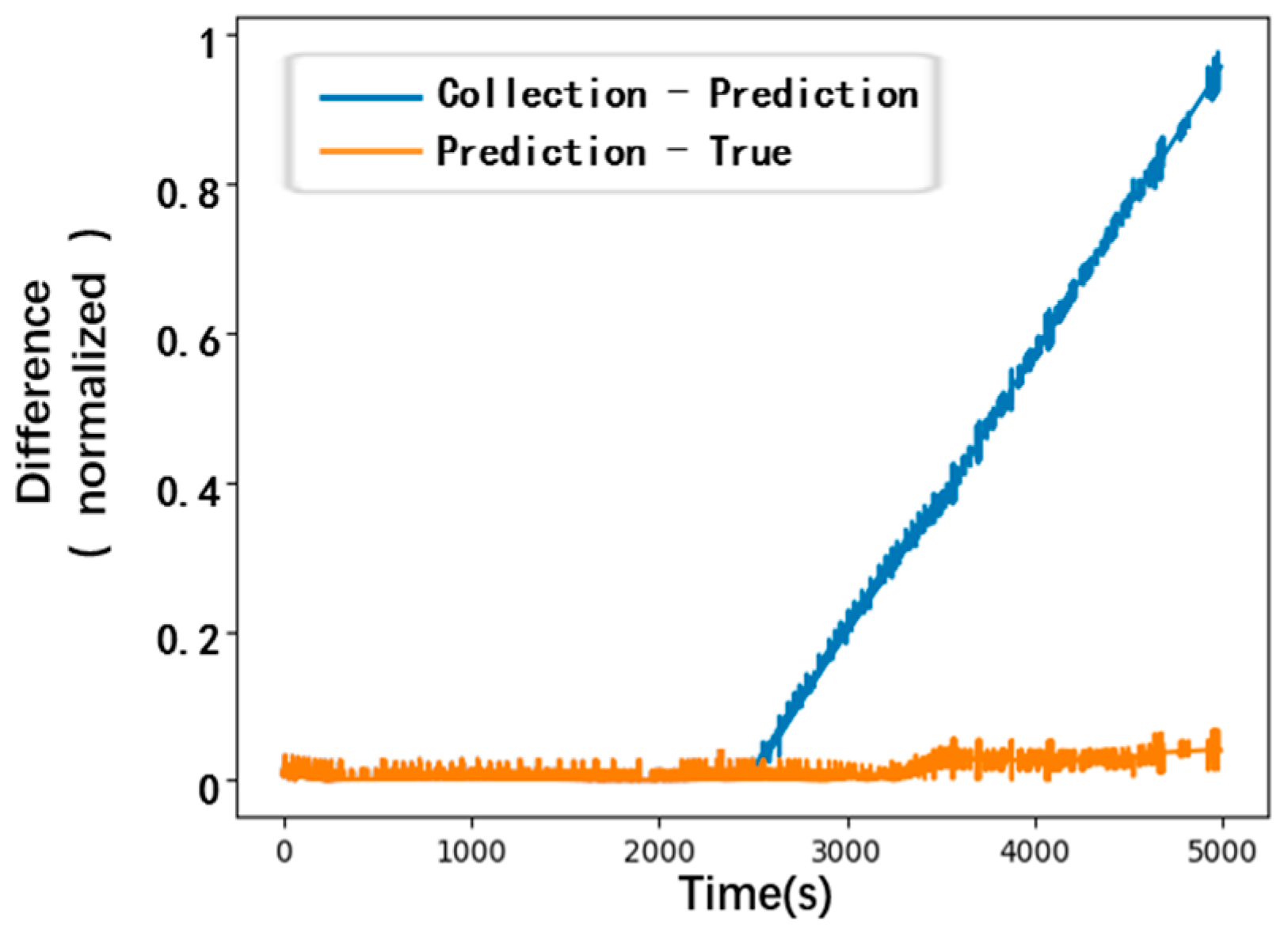
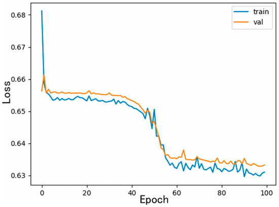
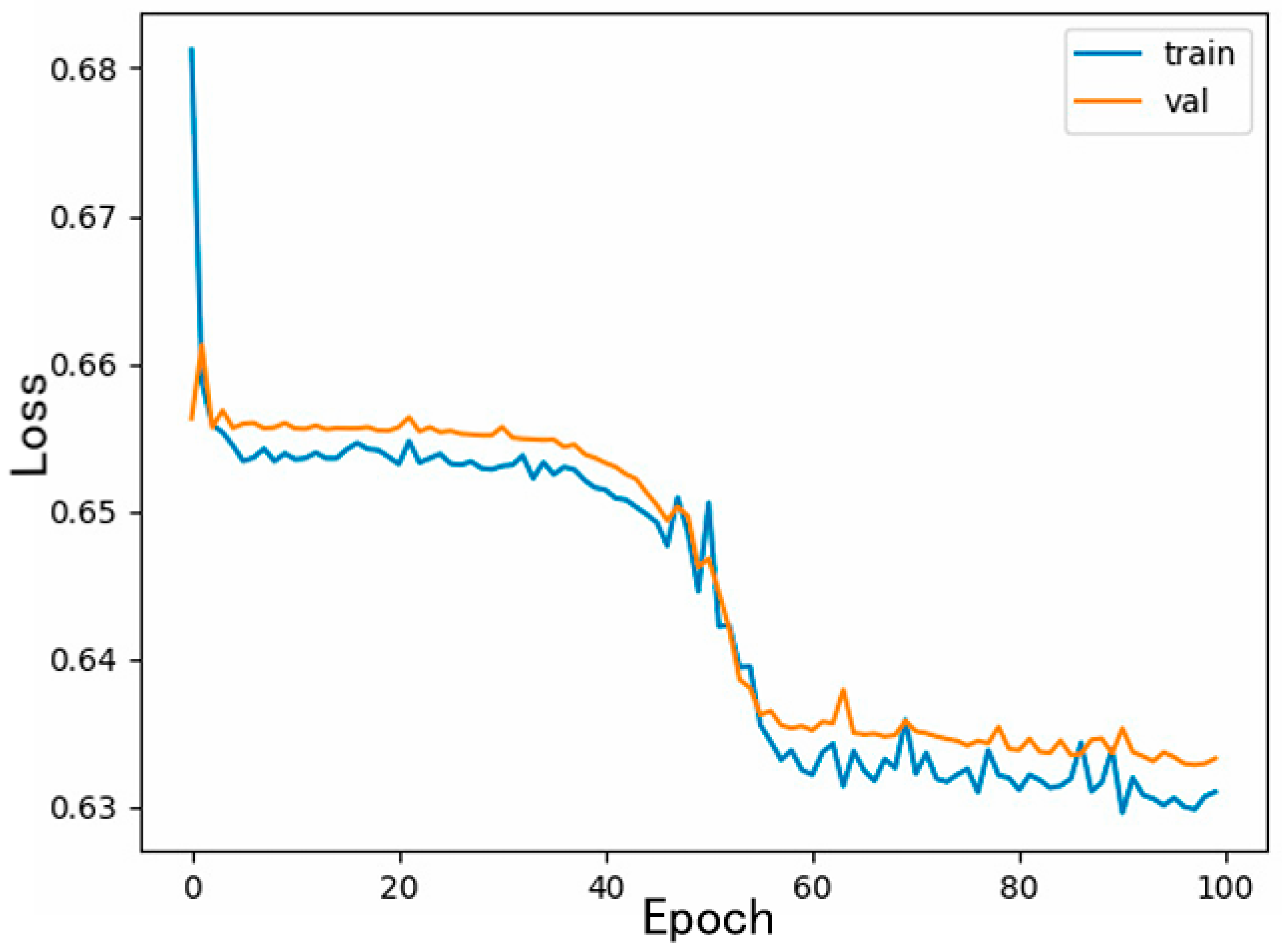
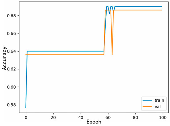
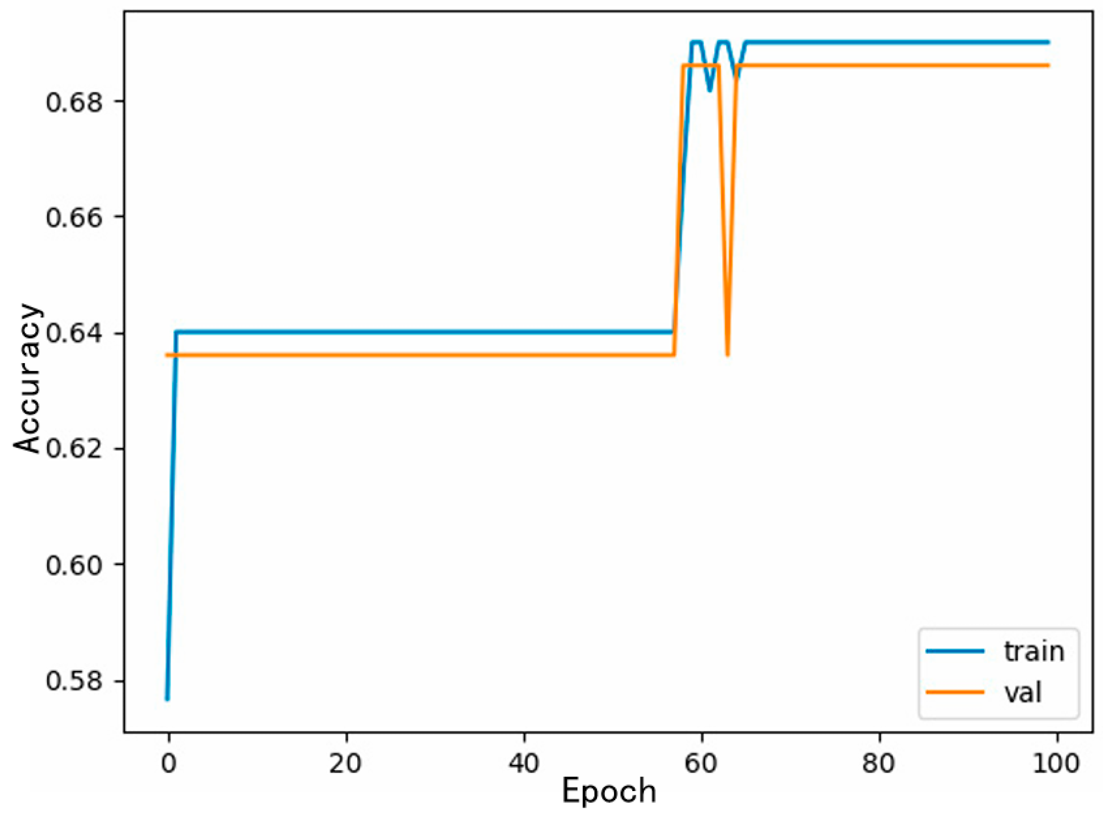
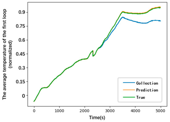
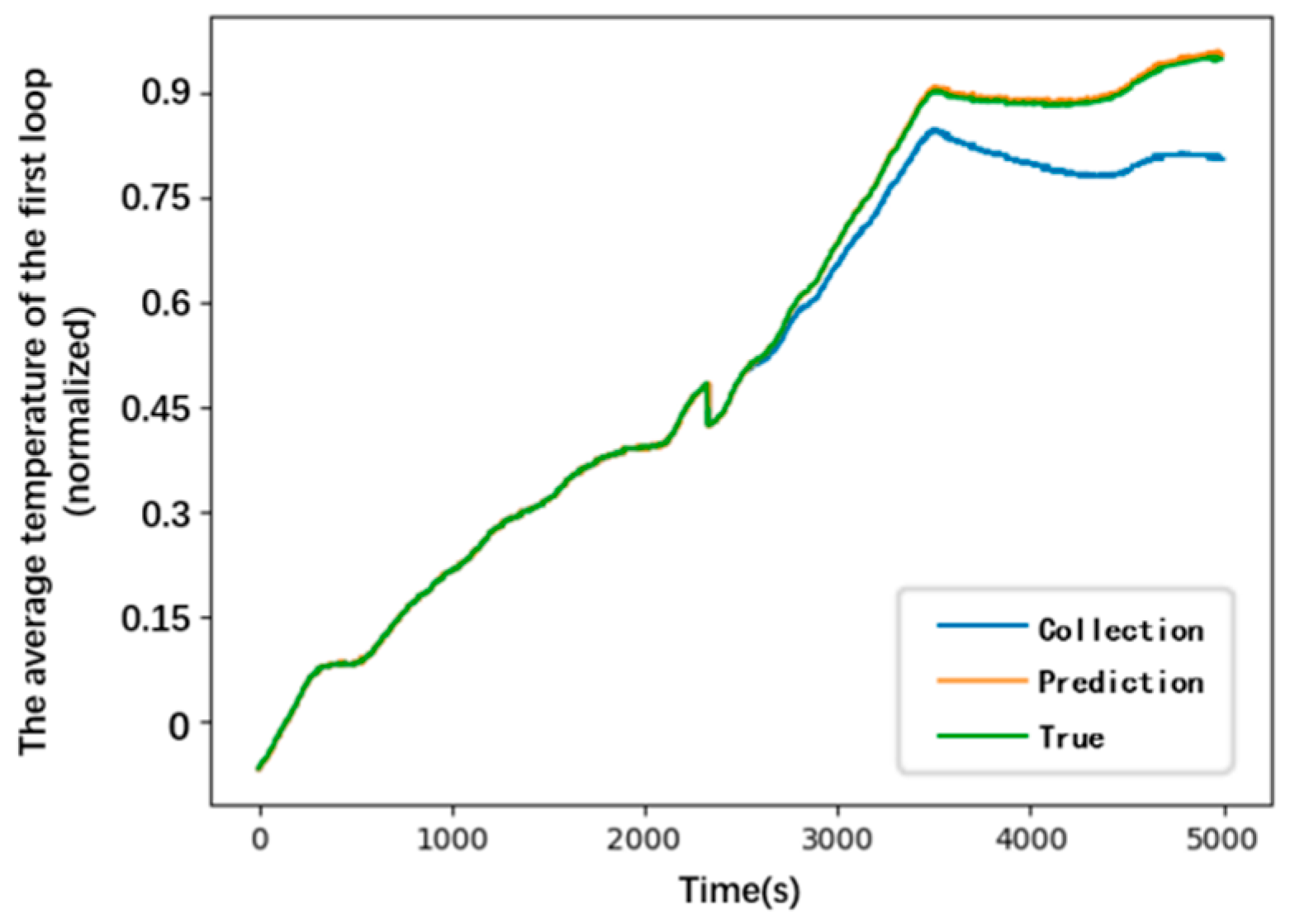
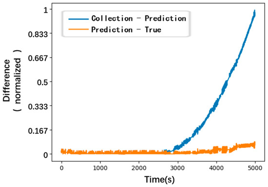
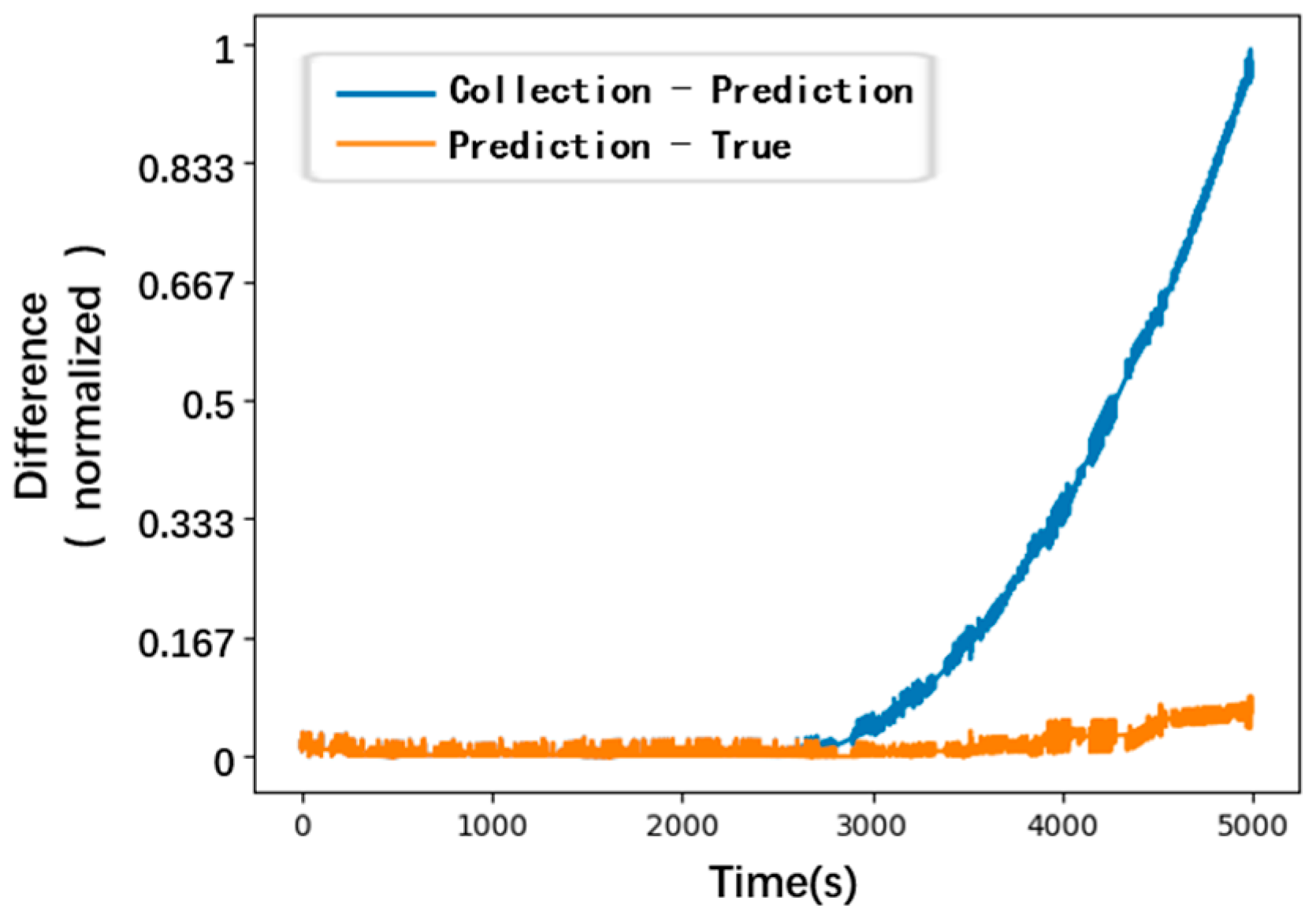
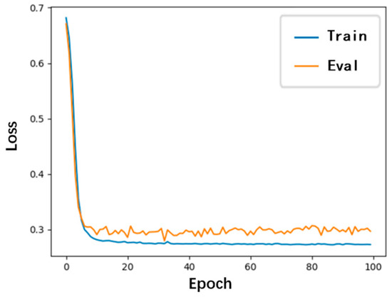
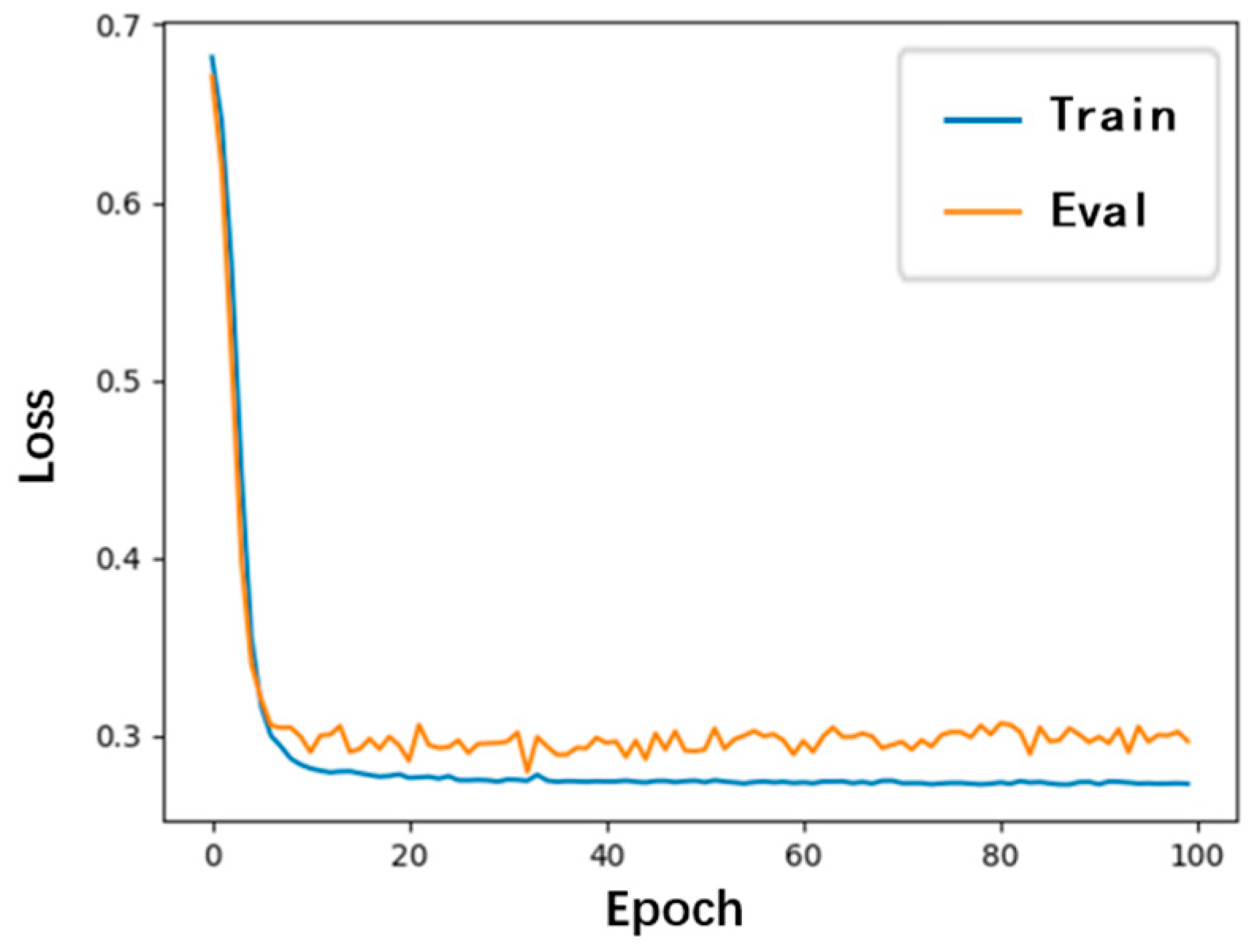
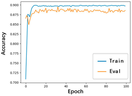
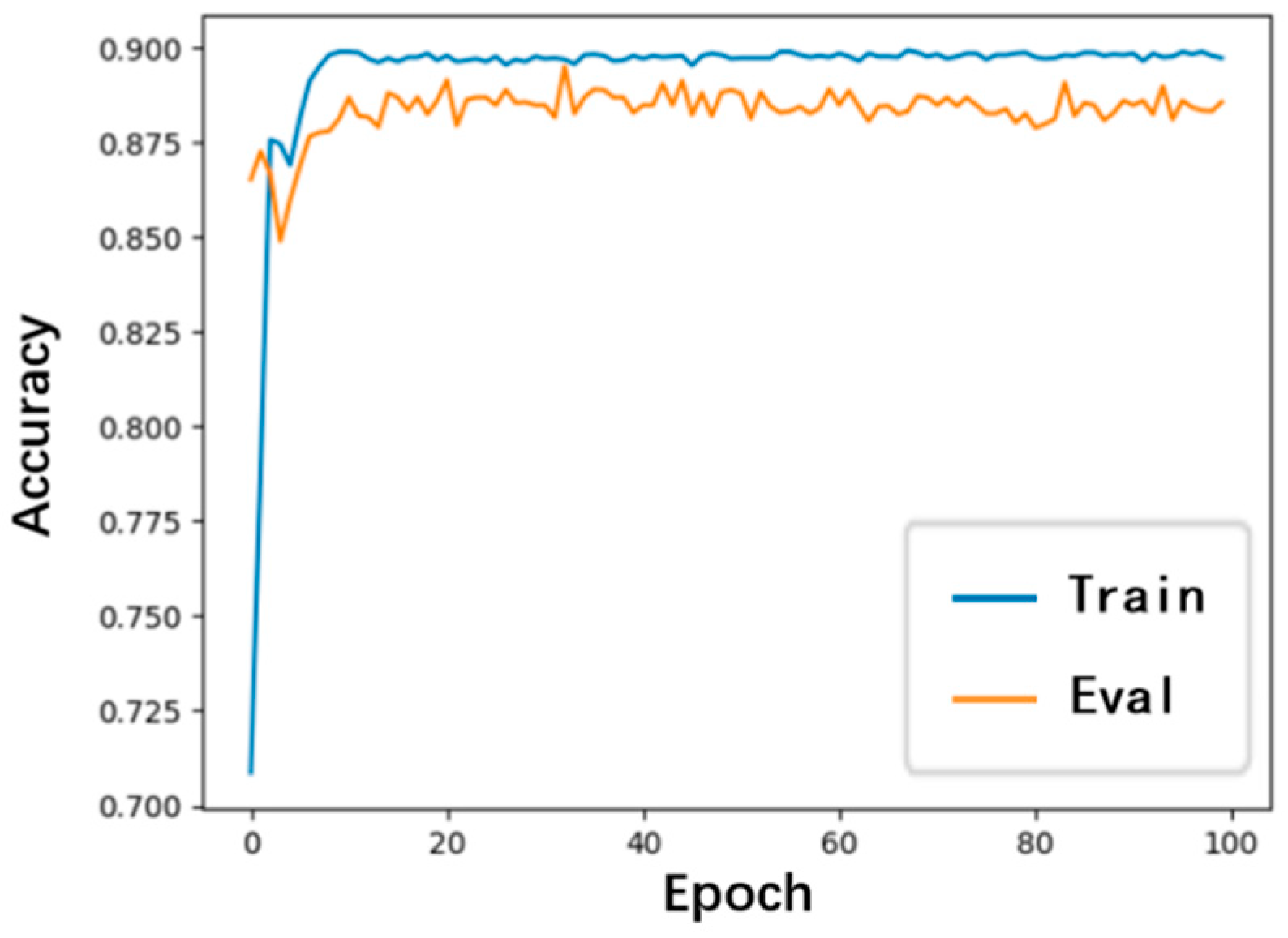
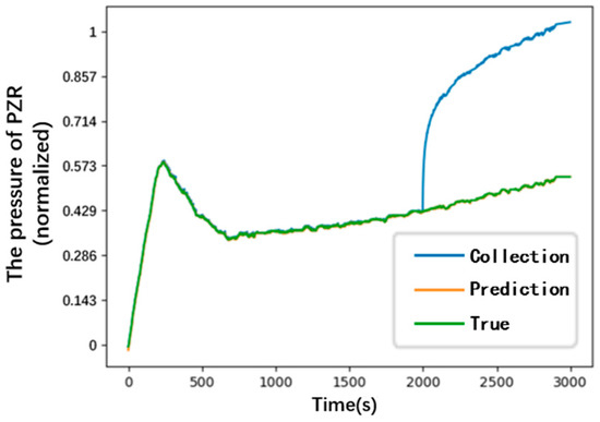
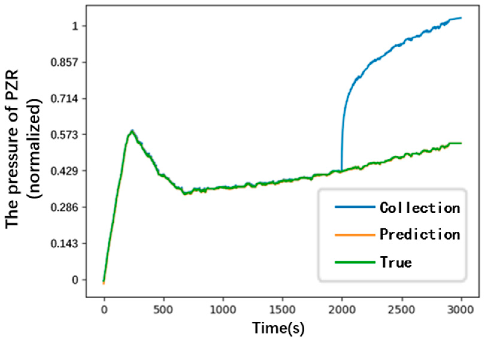
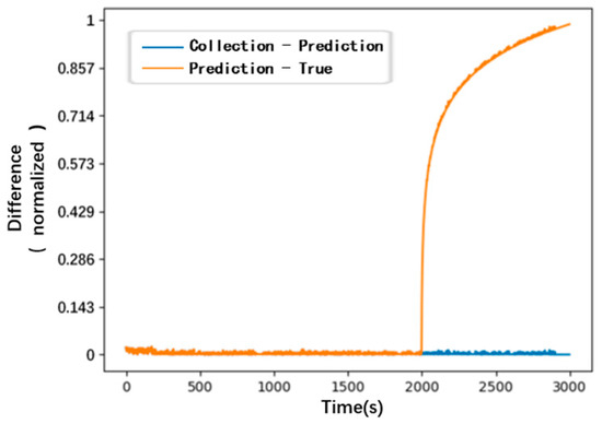
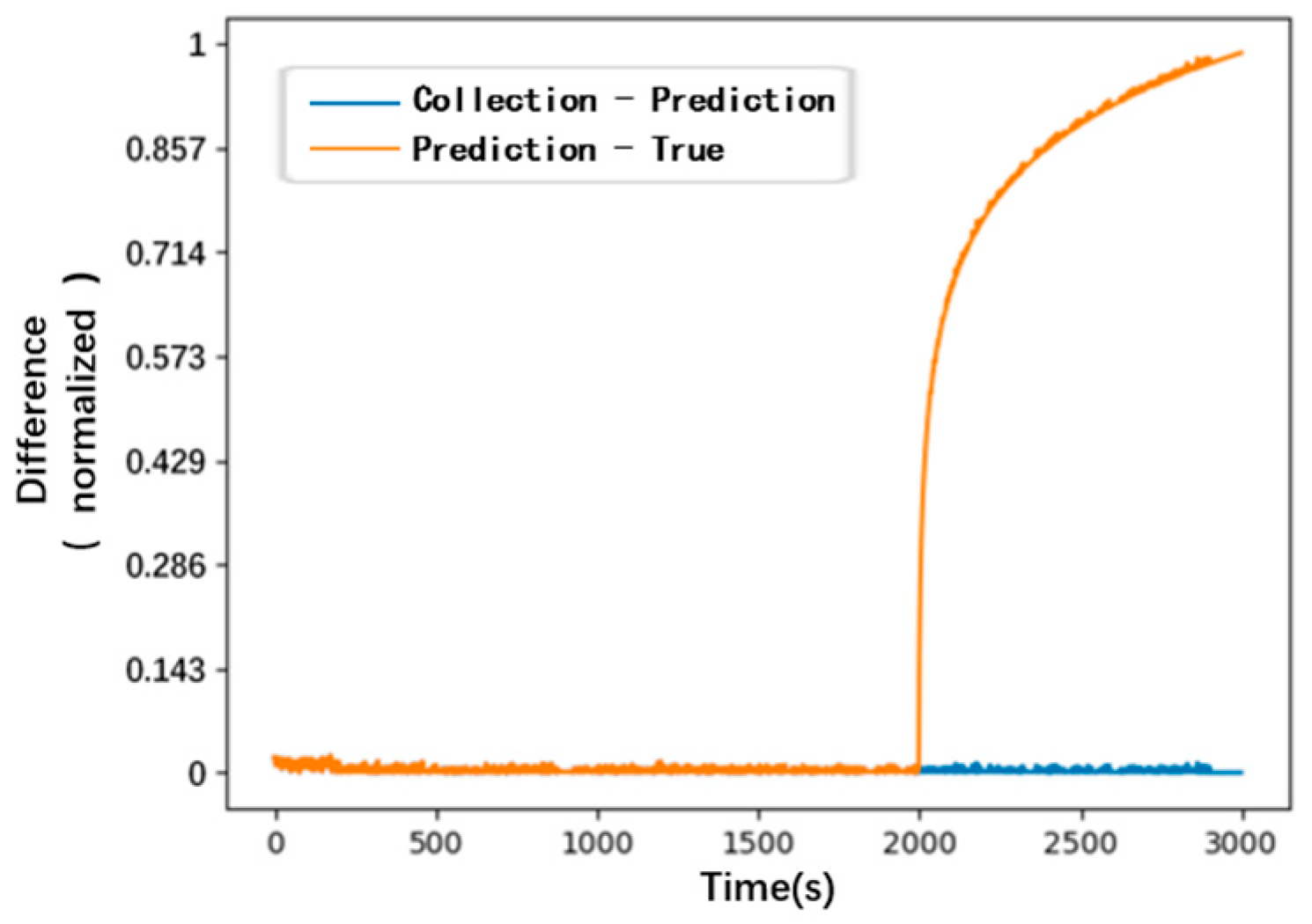
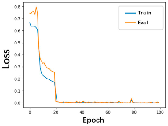
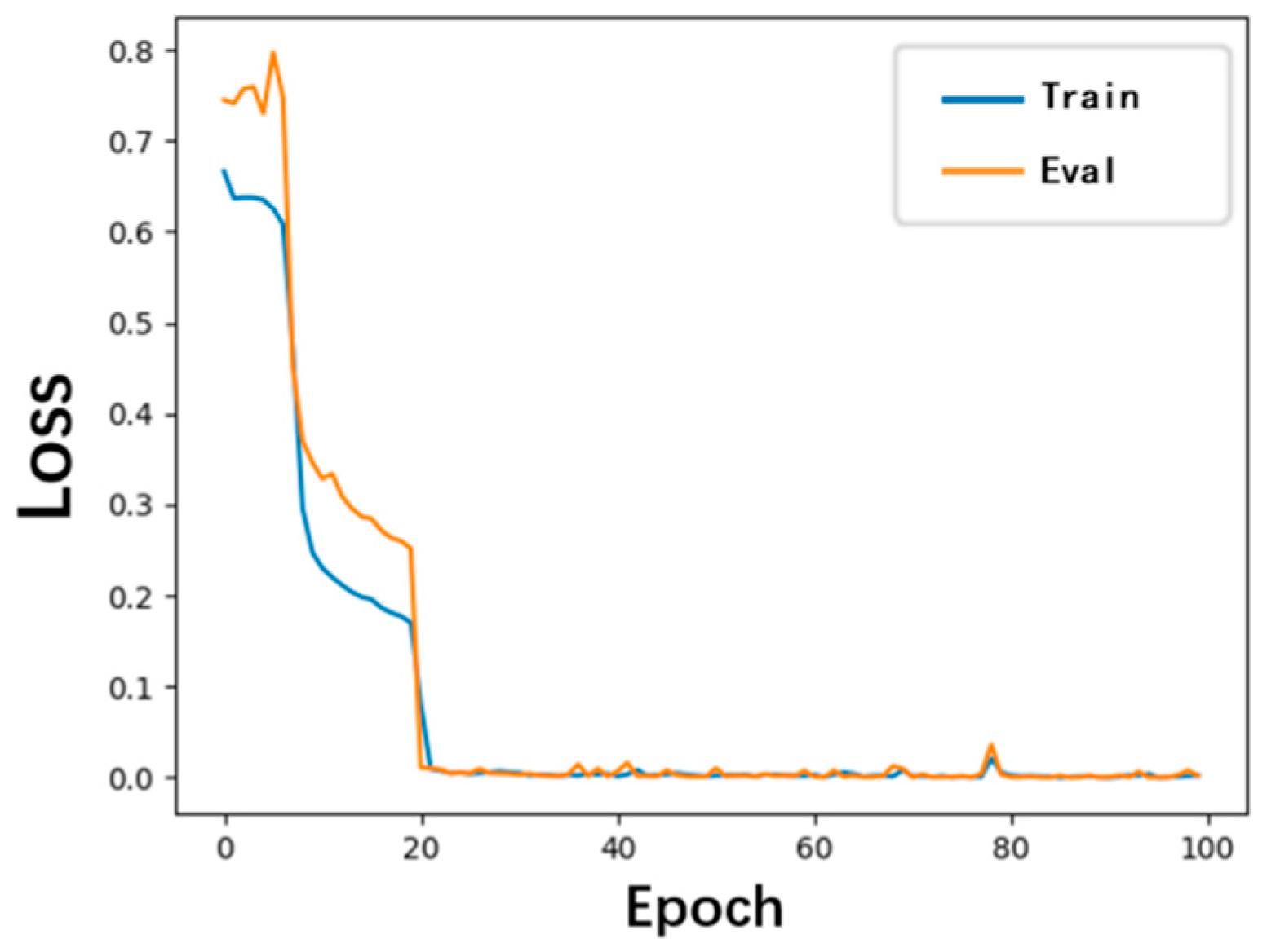
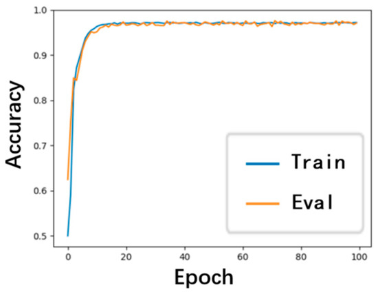
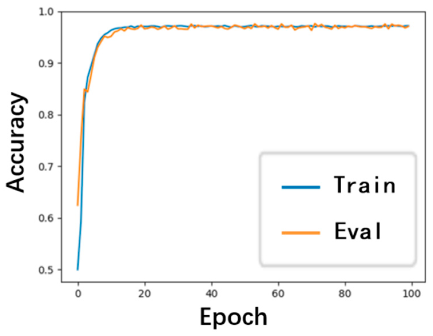
This section lists the results of the experiments carried out according to the former design. The results of each experiment are shown in four figures. In each group, the first figure (the C-P-T curve) shows the collected value, the prediction value, and the true value of the experiment data. The second figure (the C-P & P-T curve) shows the curve of the difference between the collected value and the prediction value, and the difference between the prediction value and the true value. The third figure (the L curve) shows the loss curve for the GRU-MLP model of training and evaluation. The fourth figure (the A curve) shows the accuracy curve for the GRU-MLP model of training and evaluation. Figure 22, Figure 23, Figure 24, Figure 25, Figure 26, Figure 27, Figure 28, Figure 29, Figure 30, Figure 31, Figure 32, Figure 33, Figure 34, Figure 35, Figure 36, Figure 37, Figure 38, Figure 39, Figure 40 and Figure 41 show the experimental results of each group, and the corresponding relationship is shown in Table 3.

Figure 22. The C-P-T curve for Experiment 1.

Figure 23. The C-P & P-T curve for Experiment 1.

Figure 24. The L curve for Experiment 1.

Figure 25. The A curve for Experiment 1.

Figure 26. The C-P-T curve for Experiment 2.

Figure 27. The C-P & P-T curve for Experiment 2.

Figure 28. The L curve for Experiment 2.

Figure 29. The A curve for Experiment 2.

Figure 30. The C-P-T curve for Experiment 3(a).

Figure 31. The C-P & P-T curve for Experiment 3(a).

Figure 32. The L curve for Experiment 3(a).

Figure 33. The A curve for Experiment 3(a).

Figure 34. The C-P-T curve for Experiment 3(b).

Figure 35. The C-P & P-T curve for Experiment 3(b).

Figure 36. The L curve for Experiment 3(b).

Figure 37. The A curve for Experiment 3(b).

Figure 38. The C-P-T curve for Experiment 3(c).

Figure 39. The C-P & P-T curve for Experiment 3(c).

Figure 40. The L curve for Experiment 3(c).

Figure 41. The A curve for Experiment 3(c).

Table 3. Results of the anomaly detection experiments.

Experiment Number		Anomaly Style		Experimental Results
				C-P-T Curve	C-P & P-T Curve	the L Curve	the A Curve
1		Random jump		Figure 22	Figure 23	Figure 24	Figure 25
2		Fixed-value drift		Figure 26	Figure 27	Figure 28	Figure 29
3	(a)	Growth drift	Linear growth	Figure 30	Figure 31	Figure 32	Figure 33
	(b)		Polynomial growth	Figure 34	Figure 35	Figure 36	Figure 37
	(c)		Logarithmic growth	Figure 38	Figure 39	Figure 40	Figure 41

5.3. Analysis of Anomaly Detection Experimental Results

The experimental results indicate that the proposed GRU-MLP algorithm achieves superior training and testing performance in detecting random jump and fixed-value drifts compared to growth drifts. This performance disparity can be attributed to the inherent fluctuations present in the actual data. These minor variations cause an overlap in the feature distributions used for classification, creating ambiguous regions that diminish the model’s ability to clearly distinguish gradual anomalous trends from normal operational noise, thereby compromising detection efficacy. The experimental results for the three growth drifts—linear, quadratic, and logarithmic—show a clear performance gradient, with detection efficacy improving from linear to logarithmic. This demonstrates a key principle: the masking effect of normal data variability on anomaly detection diminishes as the magnitude and rate of the anomalous drift increase. Although the detection of growth drifts exhibits minor inaccuracies, the model achieves an accuracy of approximately 90% for all three types. This represents a highly robust level of performance, demonstrating its practical utility in providing reliable decision support to plant operators.

6. Performance Comparison Experiment of Anomaly Detection Algorithms

A few comparison experiments were designed to evaluate the superiority of the proposed algorithm in detection accuracy. Two groups of comparative experiments were designed, and their details are shown in Table 4.

Table 4. Details of the performance comparison experiments among anomaly detection algorithms.

Anomaly Style	Parameter	Length of Data	Start Time of Anomaly	Number of Anomalies
Random jump	Pressure of PZR	600	randomly	100 points
Fixed-value drift		500	400	100 points

The windowed center (WinCen) value method and ARIMA method are utilized and compared with the GRU-MLP method designed. The comparison indexes are the status judgment accuracy rate and the anomaly detection rate. The experimental results are shown in Table 5 and Table 6. Among them, the status judgment accuracy rate is the ratio for the number of points correctly judged to the total amount of data. The anomaly detection rate indicates the ratio for the number of correctly detected anomalies to the total number of anomalies.

Table 5. State judgment accuracy rate.

	GRU-MLP	WinCen	ARIMA
Random anomaly	0.994	0.69	0.7633
Fixed-value drift anomaly	0.9833	0.788	0.806

Table 6. Anomaly detection rate.

	GRU-MLP	WinCen	ARIMA
Random anomaly	1	0.16	0.8
Fixed-value drift anomaly	1	0.04	0

It can be seen that the performance of the GRU-MLP method is much better than that of the other two methods, especially in the anomaly data detection rate. The reasons are briefly analyzed as follows:

(1) Compared to the WinCen and ARIMA methods, the proposed GRU-MLP algorithm introduces a key enhancement: a closed-loop correction mechanism. In this design, the predicted values are utilized to perform real-time imputation of the detected anomalies. This process mitigates the propagation of erroneous data, thereby reducing their contaminating effect on the subsequent outputs of the prediction algorithm and enhancing the overall robustness of the data stream. A critical drawback of the WinCen and ARIMA algorithms is their inability to correct anomalies, causing error propagation that compromises prediction integrity. This issue is severe during continuous anomalies like fixed-value drift. The experimental results confirm that although their predictions on normal data are accurate, their detection rates for the anomalous data itself are unacceptably low, leading to fundamentally flawed results.

(2) An inherent drawback of the WinCen and ARIMA algorithms is their dependence on a fixed detection threshold. This necessitates a conservative threshold setting to accommodate normal operational variations, inevitably resulting in a high number of undetected anomalies. Our GRU-MLP method addresses this flaw by replacing the fixed threshold with the MLP’s capability for adaptive discrimination. This optimization allows for nuanced anomaly detection that is sensitive to contextual patterns, thereby dramatically improving accuracy.

7. Experiment on Performance of Real-Time Correction Algorithm

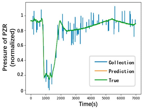
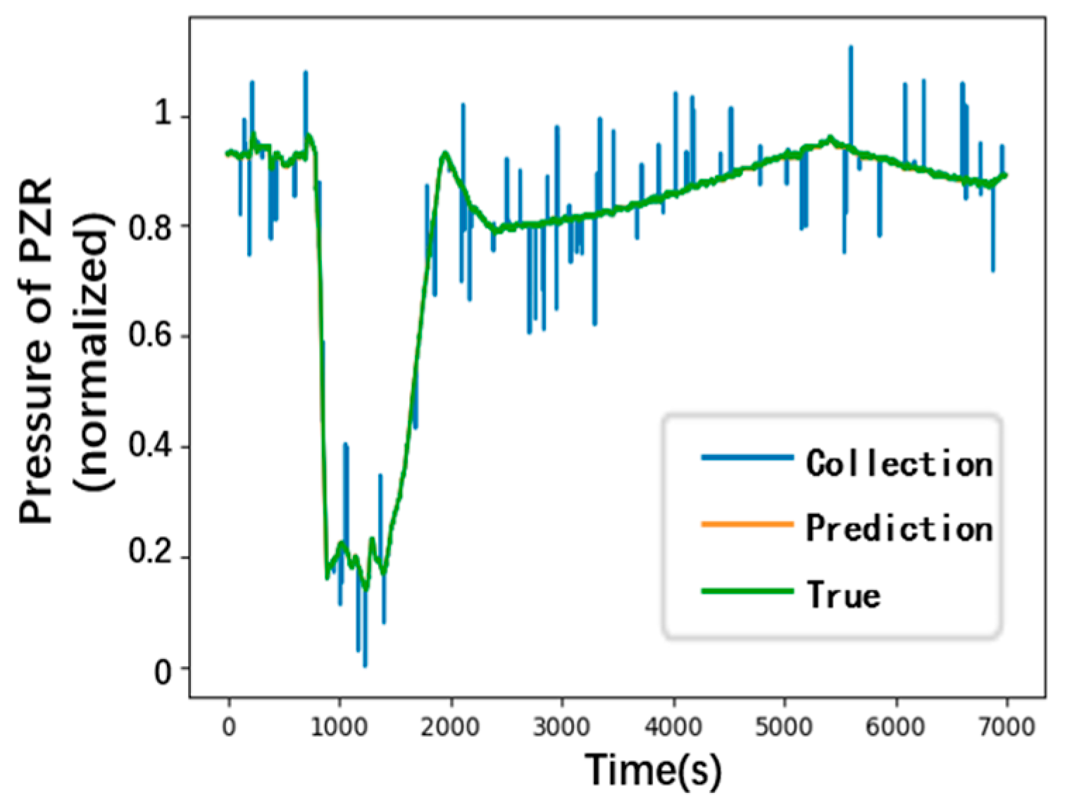
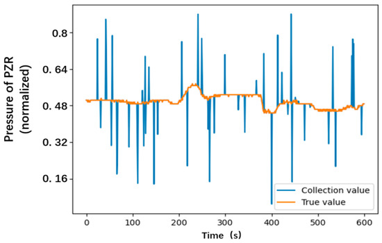
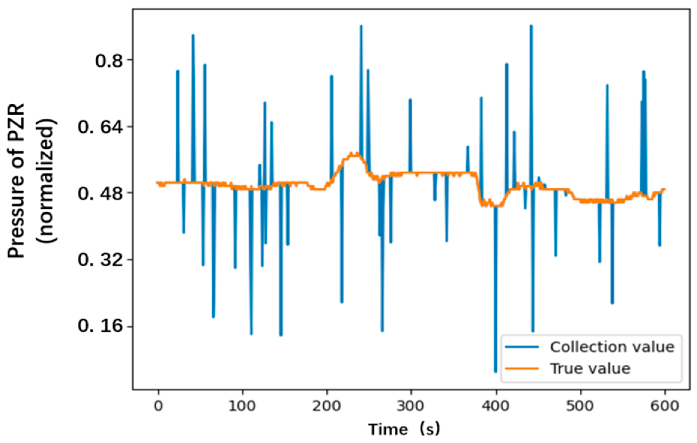
In this section, a comparative experiment is designed to verify the correction effect and important role of the real-time correction algorithm. Figure 42 shows the collected value and the true value of the pressure of PZR for a period of 600 s. This section of data is used to carry out experiments.

Figure 42. The curve of the pressure of PZR.

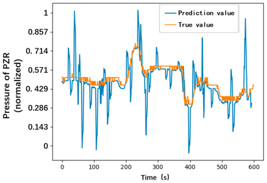
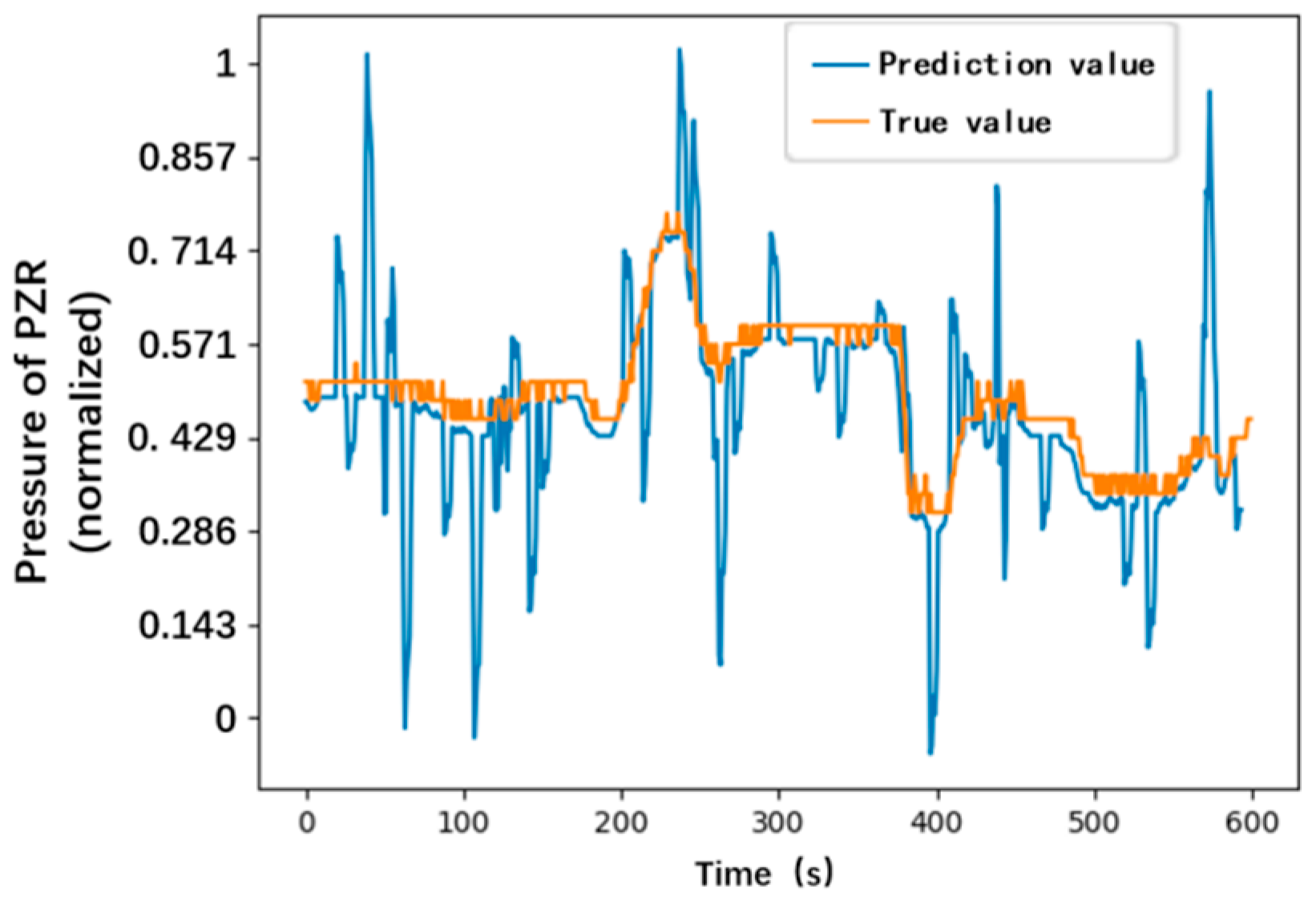
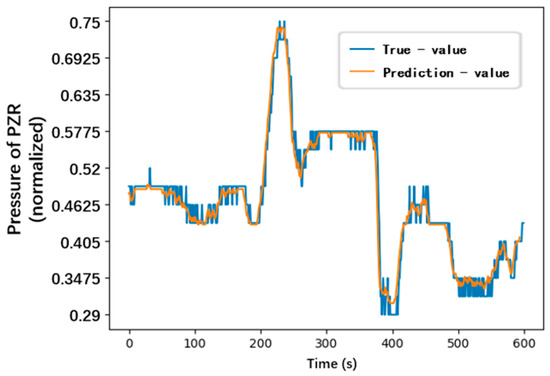
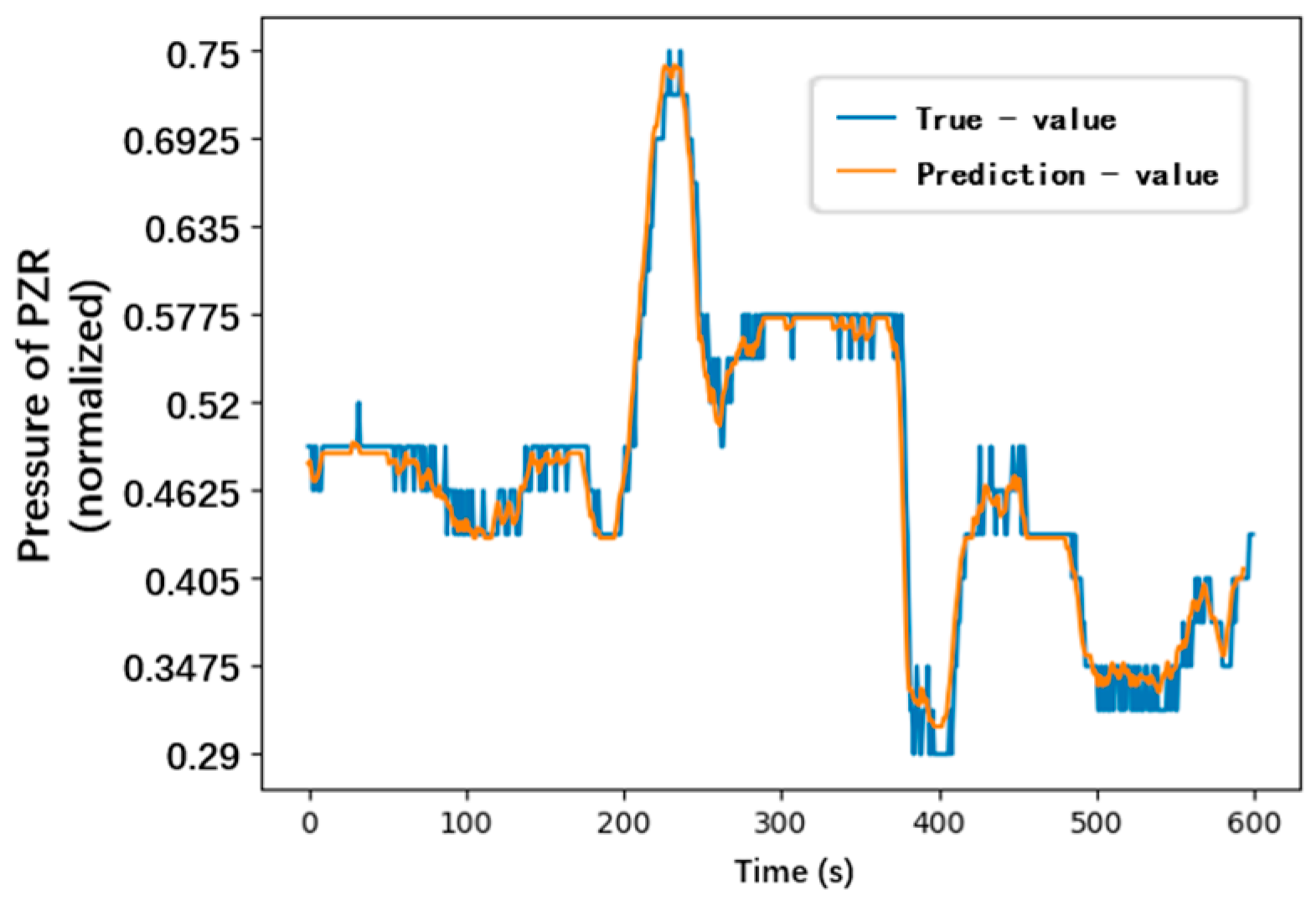
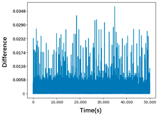
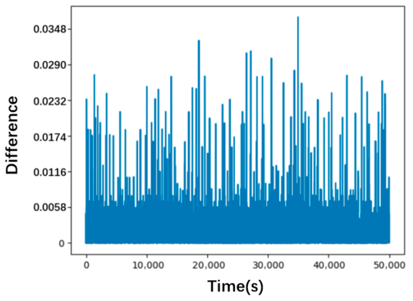
Figure 43 and Figure 44 show the comparative experimental results of the two groups. In order to highlight the comparison of the data in the two figures, the data in the two figures are normalized. Figure 43 shows the prediction effect without real-time correction using the GRU model. Figure 44 shows the prediction effect of using GRU model in the case of real-time correction for anomaly data detected during the prediction process. By comparing the experimental results of the two groups, it can be seen that the real-time correction algorithm designed in this paper can effectively reduce the interference of outliers upon the prediction effect and improve the accuracy of data prediction.

Figure 43. Prediction effect without real-time correction.

Figure 44. Prediction effect with real-time correction.

8. Research on the Migration of GRU Model for NPP

The prediction algorithm designed in this work employs a univariate forecasting strategy, where the future value of a parameter is predicted based solely on its own historical data. However, it is acknowledged that an NPP is a strongly coupled, time-varying system where operational states collectively determine the values of all parameters. This univariate approach provides a focused baseline, while the complex interdependencies present an avenue for future multi-variable modeling. Training a GRU model on NPP operational data essentially involves learning to capture and encode the characteristic patterns of plant operation from historical records. Theoretically, the trained model can be applied to predict all operational parameters. However, since different parameters are influenced to varying degrees by the plant’s operational status, model fine-tuning for specific parameters is a necessary prerequisite. This demonstrates that the GRU model possesses a strong foundational capability, or transferability, for NPP parameter prediction, which can be efficiently adapted to new tasks with minimal fine-tuning.

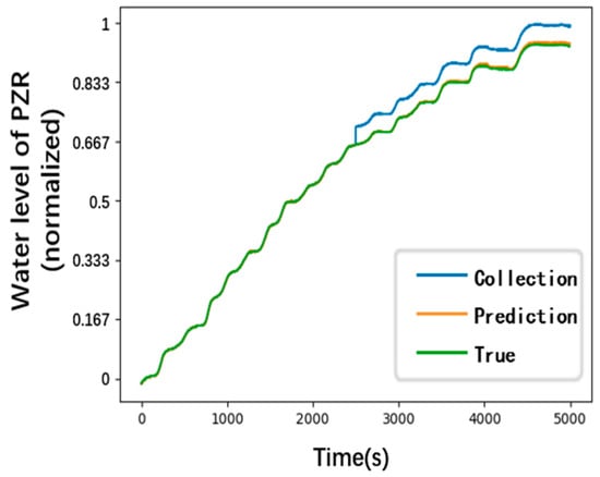
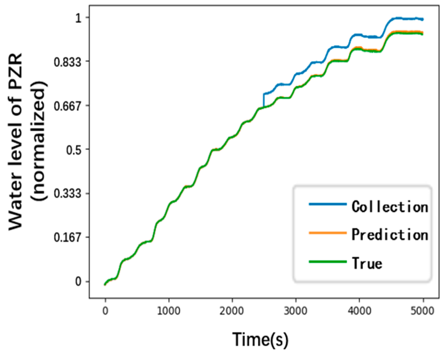
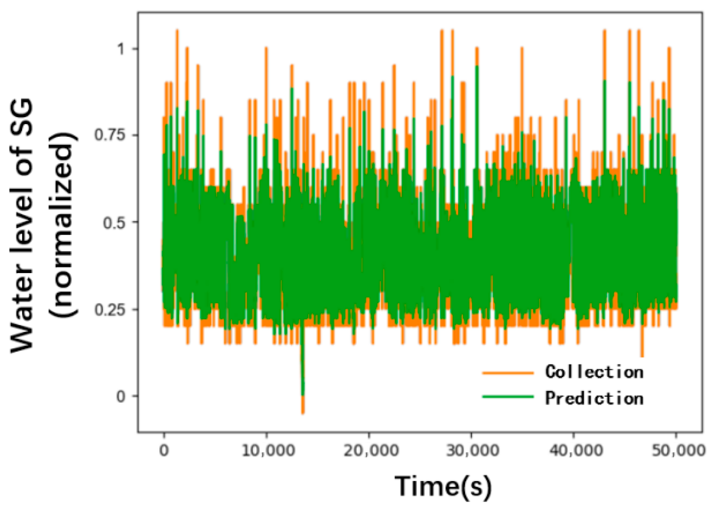
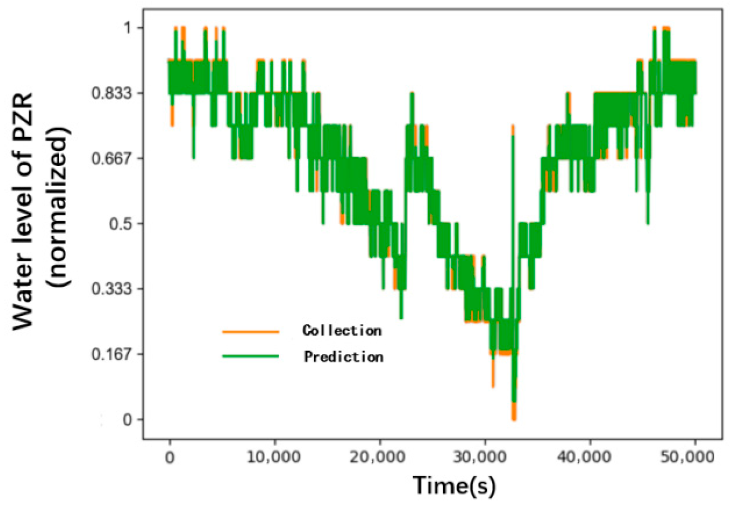
Figure 45 and Figure 46 show the direct migration of the prediction results of “the water level of SG” and “ the water level of PZR” with the model trained by the data of the pressure of PZR.

Figure 45. Migration prediction effect for water level of SG.

Figure 46. Migration prediction effect for water level of PZR.

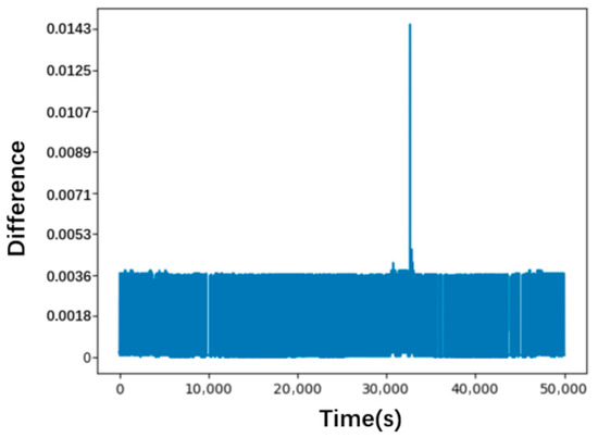
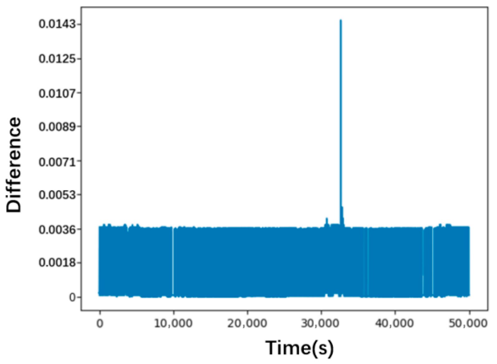
Figure 47 and Figure 48 show the curves of the differences between the predicted value and the actual value of the two parameters.

Figure 47. Migration prediction difference for water level of SG.

Figure 48. Migration prediction difference for water level of PZR.

Table 7 shows the error indexes of the migration prediction of the two parameters.

Table 7. Migration prediction difference.

Water Level of SG		Water Level of PZR
Error Index	Value	Error Index	Value
RMSE	0.34545898	RMSE	0.28555298
MSE	0.11934191	MSE	0.08154050
MAE	0.34545898	MAE	0.28555298

A comparison of the results indicates that the GRU model, trained on PZR pressure data, demonstrates superior performance in predicting the PZR water level compared to the SG water level. This disparity is attributed to the strong physical correlation between the PZR pressure and its own water level, whereas the relationship between the PZR pressure and the SG water level is comparatively weaker. The experimental results demonstrate that the GRU-based method exhibits strong transfer learning capabilities for NPP operational parameter prediction. In certain scenarios, the pre-trained model can be directly applied to predict parameters outside its original training set without any secondary training. For other tasks, it serves as an effective pre-trained foundation, significantly reducing the required training effort and computational resources, thereby enhancing overall training efficiency.

9. Conclusions

This work presents an integrated methodology for the prediction, anomaly detection, and real-time correction of NPP operational data. The proposed algorithm introduces key optimizations over traditional “prediction-detection” frameworks, primarily in two aspects. On the one hand, the real-time correction mode is added into algorithm flow so as to improve the prediction accuracy of GRU prediction algorithm for the operation data containing anomaly. On the other hand, the nonlinear fitting ability of MLP model is used to optimize the fixed threshold determination method to improve the accuracy of anomaly data detection. The correctness of the proposed algorithm and its feasibility in practical engineering application are verified by experiments with the operation data of an NPP. The prediction ability of GRU is tested, which proves the high accuracy of the GRU model in predicting operation data of NPP. The test of the GRU-MLP model’s ability to detect different anomaly patterns proves the high accuracy of the proposed algorithm in detecting anomalies of NPP operation data. Compared with the WinCen algorithm and the ARIMA algorithm, the superiority of the proposed algorithm on anomaly recognition ability was proved. The migration ability of the GRU model in NPP data prediction is demonstrated, which further improves the application value of the algorithm.

The proposed anomaly detection and correction algorithm can be deployed for both online and offline processing of NPP operational data to enhance its quality. The operational inference of the GRU-MLP pipeline is designed to be computationally lightweight, requiring only a single forward pass per time sample. This ensures that the processing latency is well within the typical sampling intervals (on the order of seconds) of I&C systems, meeting the requirements for real-time deployment. Corrected online data can be delivered directly to the human–machine interface (HMI) and simultaneously fed to the automatic control system to support autonomous and fault-tolerant control, thereby improving overall system performance. Furthermore, the validated data serve as a high-quality input for various intelligent operational support functions—such as fault diagnosis and operational guidance—enabling more accurate conclusions and thereby aiding operator observation and judgment.

It is important to note that the current study primarily validates the method using data from steady-state and normal operational conditions of a PWR. While this covers the predominant operating regime, the model’s performance in rare transients or emergency scenarios warrants further investigation. To enhance generalizability and robustness for industrial deployment, future work will focus on two key directions: (1) incorporating operational data from a broader range of plant states, including startup, shutdown, and load-following transients; and (2) exploring semi-supervised or multivariate extensions of the framework to detect more subtle, cross-dependent anomalies and unknown fault patterns.

References

- Ren, Y.; Huanlin, Z.; Huailei, Y.; Jinsong, K.; Desheng, L. Research on Abnormal Operation Status Detection Method for Nuclear Power Plants Based on Operation Data Analysis. Nucl. Power Eng. 2013, 34, 156–160. [Google Scholar]
- Wang, X.; Wang, C. Time Series Data Cleaning: A Survey. IEEE Access 2019, 8, 1866–1881. [Google Scholar] [CrossRef] [Scilit]
- Hongu, K.; Fujii, K. A simple data-driven level finding method of many-electron atoms and heavy nuclei based on statistical outlier detection. J. Phys. D Appl. Phys. 2023, 56, 244002. [Google Scholar] [CrossRef] [Scilit]
- Berendrecht, W.; van Vliet, M.; Griffioen, J. Combining statistical methods for detecting potential outliers in groundwater quality time series. Environ. Monit. Assess. 2023, 195, 85. [Google Scholar] [CrossRef] [Scilit]
- Hammad, A.; Nojiri, M.M.; Yamazaki, M. Quantum similarity learning for anomaly detection. J. High Energy Phys. 2025, 2025, 81. [Google Scholar] [CrossRef] [Scilit]
- Wang, H.; Peng, M.-J.; Yu, Y.; Saeed, H.; Hao, C.-M.; Liu, Y.-K. Fault identification and diagnosis based on KPCA and similarity clustering for nuclear power plants. Ann. Nucl. Energy 2021, 150, 107786. [Google Scholar] [CrossRef] [Scilit]
- Li, C.; Guo, L.; Gao, H.; Li, Y. Similarity-Measured Isolation Forest: Anomaly Detection Method for Machine Monitoring Data. Instrum. Meas. IEEE Trans. 2021, 70, 107786. [Google Scholar] [CrossRef] [Scilit]
- Dou, S.; Yang, K.; Jiao, Y.; Qiu, C.; Ren, K. Anomaly Detection in Event-Triggered Traffic Time Series via Similarity Learning. IEEE Trans. Dependable Secur. Comput. 2025, 22, 888–902. [Google Scholar] [CrossRef] [Scilit]
- Weller-Fahy, D.J.; Borghetti, B.J.; Sodemann, A.A. A Survey of Distance and Similarity Measures Used Within Network Intrusion Anomaly Detection. Commun. Surv. Tutor. 2015, 17, 70–91. [Google Scholar] [CrossRef] [Scilit]
- Chen, K.; Huang, L.; Ning, Q.; Guo, Y.; Li, Y. A measurement anomaly detection method on metal cartridge cases based on PointNet++. Digit. Signal Process. 2025, 161, 105120. [Google Scholar] [CrossRef] [Scilit]
- Mangé, V.; Tourneret, J.-Y.; Vincent, F.; Mirambell, L.; Vieira, F.M. Anomaly detection in ship trajectories using machine learning and dynamic time warping. Eng. Appl. Artif. Intell. 2025, 157, 111185. [Google Scholar] [CrossRef] [Scilit]
- Belis, V.; Odagiu, P.; Aarrestad, T.K. Machine learning for anomaly detection in particle physics. Rev. Phys. 2024, 12, 100091. [Google Scholar] [CrossRef] [Scilit]
- Onsu, M.A.; Simsek, M.; Fobert, M.; Kantarci, B. Intelligent multi-sensor fusion and anomaly detection in vehicles via deep learning. Internet Things 2025, 31, 101561. [Google Scholar] [CrossRef] [Scilit]
- Li, X.; Huang, T.; Cheng, K.; Qiu, Z.; Sichao, T. Research on anomaly detection method of nuclear power plant operation state based on unsupervised deep generative model. Ann. Nucl. Energy 2022, 167, 108785. [Google Scholar] [CrossRef] [Scilit]
- Fang, C.; Song, S.; Chen, Z.; Gui, A. Fine-grained fuel consumption prediction. In Proceedings of the 28th ACM International Conference on Information and Knowledge Management, Beijing, China, 3–7 November 2019; pp. 2783–2791. [Google Scholar] [CrossRef] [Scilit]
- Yingjie, S.; Minjun, P. MSET&SPRT-based Abnormal Condition Monitoring Technology for Nuclear Power Plants. Nucl. Power Eng. 2015, 36, 57–61. [Google Scholar] [CrossRef]
- Liao, J.; Yang, Y.; Liang, X. Research on Predictive Maintenance Methods for Nuclear Power Equipment Based on Artificial Intelligence. In Proceedings of the 2025 4th International Conference on Energy and Electrical Power Systems (ICEEPS), Guangzhou, China, 17–19 July 2025; pp. 718–721. [Google Scholar] [CrossRef] [Scilit]
- Zhao, M.; Chen, Z.; Liao, L.; Li, Y.; Huang, K. Research on Integrated Reactor Power Control System Based on Intelligent Prediction. Nucl. Power Eng. 2019, 40, 166–171. [Google Scholar] [CrossRef]
- Xu, Y. Research and Implementation of Fault Diagnosis and Prediction System for Nuclear Power Equipment. Master’s Thesis, Huazhong University of Science and Technology, Wuhan, China, 2019. [Google Scholar]
- Jiang, B.; Huang, X.; Hines, J.W.; Zhao, F. Prediction of Reactor Power under Accident Conditions of Nuclear Power Plant Using v-Support Vector Machine. Nucl. Power Eng. 2019, 40, 105–108. [Google Scholar] [CrossRef]
- Jiang, B.; Huang, X. Prediction of Critical Heat Flux Based on Gaussian Process Regression. Nucl. Power Eng. 2019, 40, 46–50. [Google Scholar] [CrossRef]
- Lei, J.; Xie, J.; Yu, T.; Chen, Z.; Zhao, P.; Xie, C.; Ni, Z.; Zhou, J. Study of Assembly Nuclide Density Prediction Based on Data Mining Technology. Nucl. Power Eng. 2021, 42, 126–132. [Google Scholar] [CrossRef]
- Zhang, S.; Zeng, H.; Xu, C.; Zhang, Z.; Huang, Q.; Zhang, Y.; Wang, Y.; Lu, T. Multi-Feature Fusion Multi-Step State Prediction of Nuclear Power Sensor Based on LSTM. Nucl. Power Eng. 2021, 42, 208–213. [Google Scholar] [CrossRef]
- Lipton, Z.C.; Berkowitz, J.; Elkan, C. A Critical Review of Recurrent Neural Networks for Sequence Learning. Comput. Sci. 2015, 215, 15–25. [Google Scholar] [CrossRef] [Scilit]
- Elman, J. Finding Structure in Time. Cogn. Sci. 1990, 14, 179–211. [Google Scholar] [CrossRef]
- Michael, J. Attractor Dynamics and Parallelism in a Connectionist Sequential Machine. In Proceedings of the Eighth Annual Conference of the Cognitive Science Society; IEEE: Piscataway, NJ, USA, 1986; Volume 41, pp. 531–546. [Google Scholar]
- Cho, K.; van Merriënboer, B.; Gulcehre, C.; Bahdanau, D.; Bougares, F.; Schwenk, H.; Bengio, Y. Learning Phrase Representations Using RNN Encoder-Decoder for Statistical Machine Translation. In Proceedings of the Empirical Methods in Natural Language Processing, Doha, Qatar, 25–29 October 2014; Association for Computational Linguistics: Stroudsburg, PA, USA, 2014; pp. 1724–1734. [Google Scholar]
- Tung-Bo, C.; Von-Wun, S. A Comparative Study of Recurrent Neural Network Architectures on Learning Temporal Sequences. In Proceedings of the IEEE International Conference on Neural Networks, Washington, DC, USA, 3–6 June 1996; IEEE: Piscataway, NJ, USA, 1996; pp. 1945–1950. [Google Scholar] [CrossRef] [Scilit]
- Sepp, H.; Jürgen, S. Long Short-Term Memory. Neural Comput. 1997, 9, 1735–1780. [Google Scholar] [CrossRef] [Scilit] [PubMed]
Disclaimer/Publisher’s Note: The statements, opinions and data contained in all publications are solely those of the individual author(s) and contributor(s) and not of MDPI and/or the editor(s). MDPI and/or the editor(s) disclaim responsibility for any injury to people or property resulting from any ideas, methods, instructions or products referred to in the content. |
© 2026 by the authors. Licensee MDPI, Basel, Switzerland. This article is an open access article distributed under the terms and conditions of the Creative Commons Attribution (CC BY) license.