Deep Spatiotemporal Surrogate Modeling of Natural Gas Pipeline Networks for Heterogeneous Equipment and Long-Horizon Forecasting

Abstract

Accurate multistep-ahead prediction of natural gas pipeline-network states is essential for intelligent dispatching, yet such networks contain physically heterogeneous components (gas sources, pipelines, compressors, valves), and historical states and future dispatching commands are decoupled in both temporal scale and physical semantics. This causes conventional data-driven models to suffer from semantic entanglement and cumulative error during long-horizon forecasting. This study proposes a deep spatiotemporal surrogate model with three coordinated designs: (i) type-specific feature encoding combined with global latent-graph mapping and a shared graph convolutional network (GCN) to disentangle heterogeneous-equipment attributes and represent network-wide topological coupling; (ii) a residual-gated temporal coupling mechanism that adaptively fuses historical operating inertia with future external disturbances; and (iii) a temporal-gradient multi-objective loss with a 12-step autoregressive rolling strategy over a 6 h horizon to suppress cumulative divergence. On 85,248 samples built from field monitoring data and commercial mechanistic simulations, the model attains median relative errors of 1.15% for nodal pressure and 2.10% for pipeline flow, capturing macroscopic pressure decay and high-frequency transient flow induced by valve and compressor switching without noticeable delay, providing an efficient tool for online simulation, real-time warning, and decision support in complex natural gas pipeline networks.

1. Introduction

As a clean and efficient fossil energy carrier, natural gas plays an increasingly important role in the global energy transition and carbon-neutral development. In China, the rising share of natural gas in primary energy consumption and the accelerating interregional pipeline interconnection have produced transmission and distribution systems with broader coverage, longer transport distances, and larger scales [1,2,3]. While these large networks meet growing demand, they also pose new dispatching and operation-management challenges: supply- and demand-side fluctuations driven by weather and market conditions increase load uncertainty [4,5], while frequent switching of compressors and valves makes equipment-level operating states strongly coupled and difficult to predict [6,7]. Against this background, accurate prediction of pipeline-network operating states is critical for identifying potential risks in advance and optimizing dispatching decisions [8]. Building on such predictive capabilities, multi-period integrated scheduling with underground gas storage [9], intelligent-algorithm-based operation optimization of large-scale networks [10], and steady-state optimization of the West-East Gas Pipeline [11] have been investigated, all of which rely on fast and reliable evaluation of pipeline-network operating states.

Existing operating-state prediction methods for natural gas pipeline networks can be broadly divided into two categories. The first category is mechanism-based physical modeling, which performs numerical simulation using continuity equations, momentum equations, state equations, friction laws, compressor-efficiency models, and valve characteristics. For example, Woldeyohannes et al. [12] and Herran-Gonzalez et al. [13] developed dynamic simulation models for gas transmission and distribution networks, respectively, demonstrating the advantages of mechanism-based models in terms of physical consistency and interpretability; Pambour et al. [14] established an integrated transient model for simulating the operation of gas transport systems; and Alamian et al. [15] formulated a state-space model for transient flow simulation in pipelines. However, these methods depend strongly on accurate boundary conditions and parameters, and their computational cost is high. They therefore struggle to satisfy real-time and adaptive requirements in large-scale networks subject to frequent disturbances. The second category is data-driven time-series modeling, which learns temporal dependencies from large volumes of operating data accumulated by SCADA and related systems using methods such as RNNs and LSTMs [16]. Laib et al. [17] employed LSTM recurrent neural networks for natural-gas consumption prediction, improving forecasting accuracy for efficient energy-system operation. Liu et al. [18] proposed an LSTM-based flow prediction model with grid-search parameter optimization for gas gathering and transmission pipelines; by incorporating historical and current flow information at both pipeline ends, the method improved prediction accuracy and model stability. Sharma et al. [19] further benchmarked machine-learning techniques for data-driven short-term natural gas demand forecasting. Although these approaches reduce dependence on physical parameters to some extent, they often neglect network topology and spatial correlations, making it difficult to describe the coupled evolution of multiple stations and the propagation of disturbances in complex pipeline networks.

Recent advances in deep learning for spatiotemporal modeling provide new opportunities for pipeline-network prediction: a hybrid framework integrating physics-based and data-driven methods has enabled high-accuracy online transient simulation [20], interpretable machine-learning models have been applied to dynamic network simulation [21], and autoregressive neural networks have been used to reproduce pipeline transients efficiently [22]. Graph neural networks (GNNs), which perform message passing and feature aggregation on graph structures [23], are naturally suited to pipeline systems represented by nodes, edges, and topology. Specifically, Sarkar et al. [24] enhanced GNN expressiveness in engineering networks by refining the message-passing and aggregation functions; Yang et al. [25] introduced GNNs to assign gas calorific values across a pipeline network; and Wang et al. [26] proposed a multiscale graph-based spatiotemporal network for energy-consumption prediction in gas transmission. Similar spatiotemporal-fusion ideas have proven efficient in adjacent domains: for instance, Chen et al. [27] designed a bilinear spatiotemporal fusion network that jointly models spatial and temporal correlations for accurate traffic-flow prediction, which motivates the spatiotemporal coupling strategy adopted in this work. For temporal modeling, Transformer architectures capture long-range dependencies through self-attention and have been widely applied to interpretable multi-horizon forecasting [28] and long-sequence prediction [29]; multi-channel attention variants further improve long-sequential multivariate prediction [30], and Gao et al. [31] demonstrated a zero-shot Transformer model with strong cross-condition generalization on hydraulic-actuator degradation prediction. By contrast, LSTM networks remain advantageous in capturing short-term nonstationary fluctuations and local dynamics [16,17]. Integrating GNNs with LSTM is therefore a promising strategy for jointly modeling spatial dependence, long-term trends, and short-term disturbances. Beyond purely data-driven schemes, harmonizing physical and deep-learning modeling has been shown to improve both efficiency and interpretability [32], and recent 2026 studies further show that natural-gas forecasting is moving toward uncertainty-aware and robust deep-learning schemes for pipeline-network supply assurance and sector-specific demand prediction [33,34].

Although GNN-LSTM hybrids have been explored for spatiotemporal forecasting, most existing schemes treat all nodes as homogeneous, simply concatenate historical and future features, and are trained by single-step (teacher-forcing) supervision; they therefore neglect the physical heterogeneity of pipeline equipment, the temporal-semantic mismatch between realized historical states and external future controls, and the error accumulation that dominates long-horizon rollout. To overcome these limitations, this study proposes a deep spatiotemporal surrogate model whose novelty lies in three coordinated designs. (1) Heterogeneity-aware spatial representation: instead of homogeneous regression, type-specific encoders disentangle the physical attributes of gas sources, pipelines, valves, and compressors, and a global latent-graph mapping with a shared GCN explicitly represents network-wide topological coupling. (2) Residual-gated temporal coupling: a dynamic gating mechanism adaptively quantifies and fuses historical operating inertia with future dispatching disturbances, resolving feature injection when historical states and external controls differ in both temporal length and physical semantics, yielding an interpretable gate not provided by conventional GNN-LSTM models. (3) Long-horizon stabilization: a temporal-gradient multi-objective loss combined with a 12-step autoregressive rolling training strategy explicitly penalizes cumulative divergence over a 6 h prediction window. Together, these designs distinguish the proposed model from generic spatiotemporal forecasters and yield a high-fidelity, low-latency data-driven surrogate for complex continuous dispatching scenarios.

2. Methodology

This section presents the proposed deep spatiotemporal surrogate model, focusing on three major challenges: complex topological coupling, heterogeneity among pipeline-network components, and accumulated error in multistep rollout. We first formulate the spatiotemporal prediction problem for heterogeneous network elements and present the overall architecture. We then describe four core network mechanisms: historical-state encoding, future-control encoding, dynamic gated coupling, and type-specific prediction decoding. Finally, we introduce a composite loss function with temporal-gradient constraints and an autoregressive rolling training strategy to improve robustness in long-horizon forecasting.

2.1. Problem Formulation and Overall Architecture

Prediction of natural gas pipeline-network operating states is essentially a spatiotemporal dynamic modeling problem jointly driven by topological constraints, historical operating-state memory, and multidimensional future dispatching commands such as gas-source allocation and compressor speed regulation. The model must therefore represent the interactions among spatial topological coupling, historical-state inertia, and future-control forcing. In addition, gas sources, pipelines, valves, and compressor units exhibit substantial physical heterogeneity in their input and output dimensions. Conventional homogeneous feature concatenation can easily damage the operational semantics of specific equipment types. This study therefore establishes a modeling paradigm of type-specific feature encoding and global latent graph mapping, in which the implicit features of each component type are reconstructed into a unified pipeline-network topology while preserving their type-dependent physical differences. This enables accurate modeling of network-wide complex spatiotemporal evolution.

To express the heterogeneous system mathematically, we first define the core variables and notation. Let the pipeline-network topology be $\mathcal{G}=(\mathcal{V},\mathcal{E})$, with $N=\left|\mathcal{V}\right|$ nodes and $K$ physical component types. Along the temporal dimension, the historical observation length and future prediction length are denoted by $T_{in}$ and $T_{out}$, respectively. In the feature dimension, $F_k^{hist}$, $F_k^{ctrl}$, and $F_k^{out}$ denote the dimensions of the historical input, future control, and prediction output for type-$k$ nodes, respectively.

Based on these definitions, the spatiotemporal tensor spaces of different node types can be specified rigorously. For type-$k$ nodes, the historical input tensor is ${\mathbf{X}}_k^{hist}\in {\mathbb{R}}^{N_k\times T_{in}\times F_k^{hist}}$. For the controlled-node set ${\mathcal{K}}_c$, the future-control tensor ${\mathbf{U}}_k^{fut}\in {\mathbb{R}}^{N_k\times T_{out}\times F_k^{ctrl}}$ is constructed from external dispatching commands, with zero-vector padding applied to uncontrolled nodes. For the output-node set ${\mathcal{K}}_y$, the model output is the prediction set $\widehat{\mathcal{Y}}=\{{\widehat{\mathbf{Y}}}_k\in {\mathbb{R}}^{N_k\times T_{out}\times F_k^{out}}\mid k\in {\mathcal{K}}_y\}$, which jointly contains type-specific physical quantities such as pressure and flow. Accordingly, multistep spatiotemporal prediction of the pipeline network can be formulated as the following nonlinear mapping, as shown in Equation (1):

$${\widehat{\mathcal{Y}}}_{t+1:t+T_{\mathrm{o}\mathrm{u}\mathrm{t}}}=f_{\theta }\left({\mathcal{X}}_{t-T_{\mathrm{i}\mathrm{n}}+1:t}^{\mathrm{h}\mathrm{i}\mathrm{s}\mathrm{t}},{\mathcal{U}}_{t+1:t+T_{\mathrm{o}\mathrm{u}\mathrm{t}}}^{\mathrm{f}\mathrm{u}\mathrm{t}},\mathcal{G}\right)$$

(1)

where $f_{\theta }$ is the deep spatiotemporal surrogate network to be learned. This output form ensures that gas-source/user nodes output pressure, ordinary nodes output pressure, pipelines output inlet and outlet flows, and compressor stations output flow. Control-oriented objects such as valves and regulating valves participate only as future-control inputs and are not treated as independent prediction outputs, thereby aligning the model outputs with practical engineering requirements.

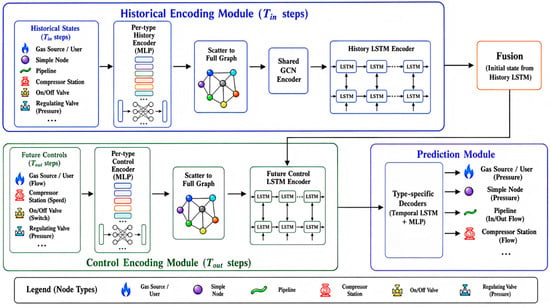
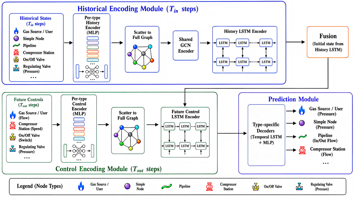
In the experiments, the data sampling interval is set to 30 min; that is, $T_{in}=4$ corresponds to a 2 h historical observation window, and $T_{out}=2$ corresponds to a 1 h prediction window. This setting creates unequal sequence lengths between historical inputs and prediction outputs, and the variables also differ fundamentally in physical semantics: historical states are realized operating outcomes, whereas future controls are external driving conditions. Under this joint temporal and semantic heterogeneity, conventional feature concatenation and unified regression architectures cannot adequately capture the dynamic coupling between the two. To overcome this limitation, the deep spatiotemporal surrogate architecture shown in Figure 1 is constructed. The model consists of four collaborative modules: a historical-state encoding module, which extracts implicit spatiotemporal memory from the full-network topology and operating-state evolution; a future-control encoding module, which extracts dynamic driving features from external dispatching commands; a dynamic gated coupling module, which adaptively fuses historical inertia and future disturbances to resolve matching between unequal sequences and heterogeneous variables; and a type-specific prediction decoding module, which independently decodes outputs according to the physical semantics of each equipment type after full-graph spatiotemporal coupling in the latent space. The architecture preserves physical boundaries and operational logic while efficiently capturing the spatiotemporal evolution of complex pipeline networks.

Figure 1. Overall architecture of the pipeline-network surrogate model.

2.2. Deep Spatiotemporal Surrogate Model

2.2.1. Historical-State Encoding Module

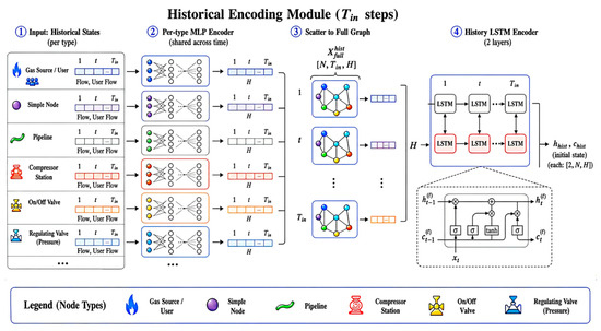
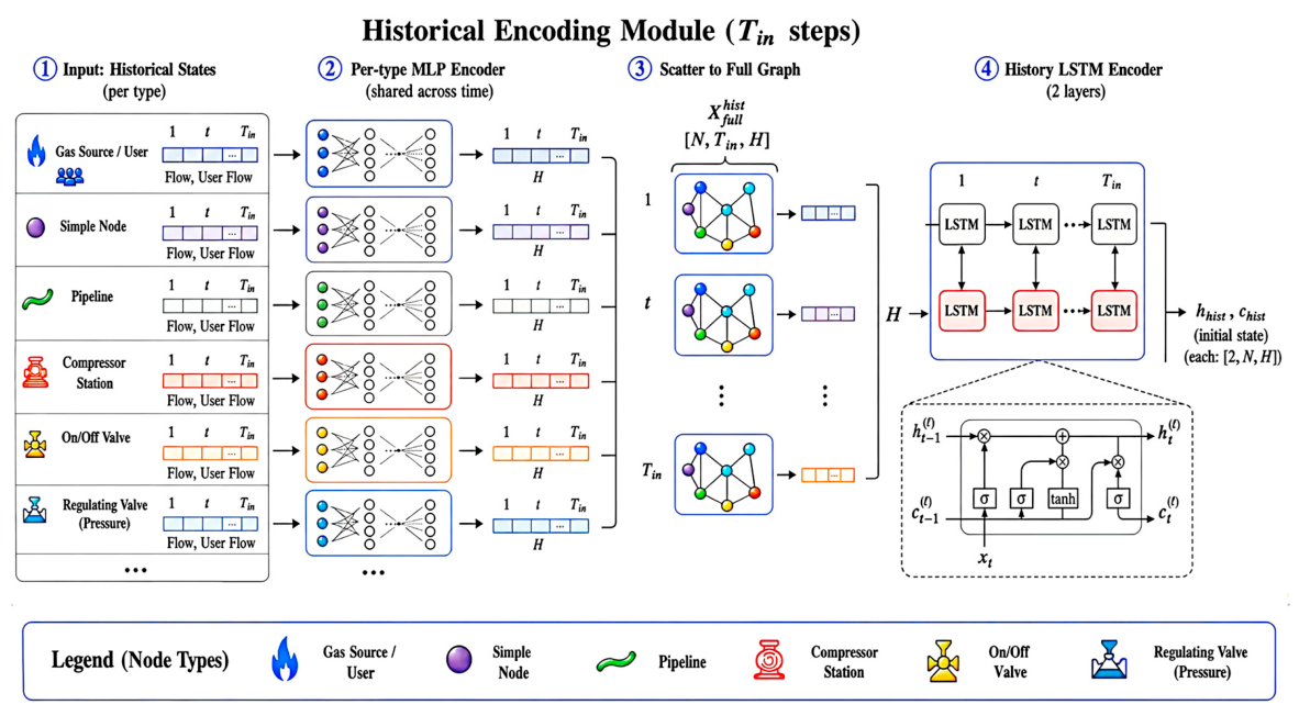
The historical-state encoding module converts the pipeline-network operating states over the previous $T_{in}$ time steps into implicit spatiotemporal memory that represents the current operating condition. As shown in Figure 2, the module receives historical-state sequences from different operational object types and outputs full-graph historical hidden and memory states, which serve as the initial operating condition for subsequent future-control fusion and prediction decoding.

Figure 2. Schematic of the historical-state encoding module.

Let the historical input tensor of type-$\mathrm{k}$ nodes be ${\mathrm{X}}_{\mathrm{k}}^{\mathrm{h}\mathrm{i}\mathrm{s}\mathrm{t}}=\left[{\mathrm{x}}_{\mathrm{k},1}^{\mathrm{h}\mathrm{i}\mathrm{s}\mathrm{t}},{\mathrm{x}}_{\mathrm{k},2}^{\mathrm{h}\mathrm{i}\mathrm{s}\mathrm{t}},\dots ,{\mathrm{x}}_{\mathrm{k},{\mathrm{T}}_{\mathrm{i}\mathrm{n}}}^{\mathrm{h}\mathrm{i}\mathrm{s}\mathrm{t}}\right]\in {\mathbb{R}}^{{\mathrm{N}}_{\mathrm{k}}\times {\mathrm{T}}_{\mathrm{i}\mathrm{n}}\times {\mathrm{F}}_{\mathrm{k}}^{\mathrm{h}\mathrm{i}\mathrm{s}\mathrm{t}}}$. A type-specific multilayer perceptron (MLP) with parameters shared along the temporal dimension is introduced to map this tensor nonlinearly into a unified latent space, as shown in Equation (2):

$$Z_k^{\mathrm{h}\mathrm{i}\mathrm{s}\mathrm{t}}={\varphi }_k^{\mathrm{h}\mathrm{i}\mathrm{s}\mathrm{t}}\left(X_k^{\mathrm{h}\mathrm{i}\mathrm{s}\mathrm{t}}\right), Z_k^{\mathrm{h}\mathrm{i}\mathrm{s}\mathrm{t}}\in {\mathbb{R}}^{N_k\times T_{\mathrm{i}\mathrm{n}}\times H}$$

(2)

where ${\mathsf{\varphi }}_{\mathrm{k}}^{\mathrm{h}\mathrm{i}\mathrm{s}\mathrm{t}}(\cdot )$ denotes the type-specific historical encoder for type-$\mathrm{k}$ nodes, and $\mathrm{H}$ is the common latent dimension. The encoder contains multiple linear projection and nonlinear activation layers, enabling the model to extract type-specific dynamic features while unifying the global feature dimension.

Because independent encoding can isolate information among nodes, the true physical topological coupling of the pipeline network must be restored. After within-type feature encoding, a node-index mapping matrix ${\mathrm{S}}_{\mathrm{k}}\in \{\mathrm{0,1}{\}}^{\mathrm{N}\times {\mathrm{N}}_{\mathrm{k}}}$ is introduced to scatter the encoded latent vectors of each node type back to their original positions in the full graph, as shown in Equation (3):

$$X_{\mathrm{f}\mathrm{u}\mathrm{l}\mathrm{l}}^{\mathrm{h}\mathrm{i}\mathrm{s}\mathrm{t}}={\displaystyle \sum _{k=1}^K}{S}_k{Z}_k^{\mathrm{h}\mathrm{i}\mathrm{s}\mathrm{t}}$$

(3)

where ${\mathrm{X}}_{\mathrm{f}\mathrm{u}\mathrm{l}\mathrm{l}}^{\mathrm{h}\mathrm{i}\mathrm{s}\mathrm{t}}\in {\mathbb{R}}^{\mathrm{N}\times {\mathrm{T}}_{\mathrm{i}\mathrm{n}}\times \mathrm{H}}$ denotes the latent-space features. Based on this global tensor, the model uses a graph convolutional network with shared weights to analyze spatial propagation patterns of pipeline-network states at each time step. Let the full-graph node representation at time $\mathrm{t}$ be ${\mathrm{X}}_{\mathrm{t}}^{\mathrm{h}\mathrm{i}\mathrm{s}\mathrm{t}}={\mathrm{X}}_{\mathrm{f}\mathrm{u}\mathrm{l}\mathrm{l}}^{\mathrm{h}\mathrm{i}\mathrm{s}\mathrm{t}}[:,\mathrm{t},:]$. Its spectral-domain approximation can be expressed as shown in Equation (4):

$$G_t^{\mathrm{h}\mathrm{i}\mathrm{s}\mathrm{t}}=\rho \left({\tilde{D}}^{-{\displaystyle \frac{1}{2}}}\tilde{A}{\tilde{D}}^{-{\displaystyle \frac{1}{2}}}{X}_t^{\mathrm{h}\mathrm{i}\mathrm{s}\mathrm{t}}{W}_g\right)$$

(4)

where $\tilde{\mathrm{A}}=\mathrm{A}+\mathrm{I}$ is the adjacency matrix with self-connections, $\tilde{\mathrm{D}}$ is the corresponding degree matrix, ${\mathrm{W}}_{\mathrm{g}}$ is a learnable parameter matrix, and $\mathsf{\rho }(\cdot )$ is the activation function. From the perspective of a local node $\mathrm{i}$, the graph aggregation process can be written as shown in Equation (5):

$$g_{i,t}^{\mathrm{h}\mathrm{i}\mathrm{s}\mathrm{t}}=\rho \left(\sum _{j\in \mathcal{N}\left(i\right)\cup \left\{i\right\}}{\displaystyle \frac{1}{\sqrt{{\tilde{d}}_i{\tilde{d}}_j}}}{x}_{j,t}^{\mathrm{h}\mathrm{i}\mathrm{s}\mathrm{t}}{W}_g\right)$$

(5)

where $\mathcal{N}\left(\mathrm{i}\right)$ is the first-order topological neighborhood of node $\mathrm{i}$. This expression characterizes the physical coupling by which pressure fluctuations and flow variations propagate from one node to neighboring nodes through pipeline connections. The shared-weight design further enforces temporal translation invariance in spatial propagation.

After spatial information has been enhanced, a two-layer long short-term memory (LSTM) network is introduced to extract the temporal evolution and state-transition memory of pipeline operating conditions over the previous 2 h, as shown in Equation (6):

$$R^{\mathrm{h}\mathrm{i}\mathrm{s}\mathrm{t}},(h^{\mathrm{h}\mathrm{i}\mathrm{s}\mathrm{t}},c^{\mathrm{h}\mathrm{i}\mathrm{s}\mathrm{t}})={\mathrm{L}\mathrm{S}\mathrm{T}\mathrm{M}}_{\mathrm{h}\mathrm{i}\mathrm{s}\mathrm{t}}\left(G^{\mathrm{h}\mathrm{i}\mathrm{s}\mathrm{t}}\right)$$

(6)

where ${\mathrm{R}}^{\mathrm{h}\mathrm{i}\mathrm{s}\mathrm{t}}\in {\mathbb{R}}^{\mathrm{N}\times {\mathrm{T}}_{\mathrm{i}\mathrm{n}}\times \mathrm{H}}$ is the sequence of hidden states output by the LSTM at each time step, and ${\mathrm{h}}^{\mathrm{h}\mathrm{i}\mathrm{s}\mathrm{t}}$ and ${\mathrm{c}}^{\mathrm{h}\mathrm{i}\mathrm{s}\mathrm{t}}$ are the final hidden state and cell state, respectively.

The module outputs two key quantities to the subsequent forecasting framework. First, the two-layer final state of the historical LSTM is directly assigned as the initial operating environment of the future decoder (${\mathrm{h}}_0^{\mathrm{d}\mathrm{e}\mathrm{c}}={\mathrm{h}}^{\mathrm{h}\mathrm{i}\mathrm{s}\mathrm{t}},{\mathrm{c}}_0^{\mathrm{d}\mathrm{e}\mathrm{c}}={\mathrm{c}}^{\mathrm{h}\mathrm{i}\mathrm{s}\mathrm{t}}$), which preserves strict continuity of the fluid-system trajectory at the latent-state level. Second, the terminal contextual feature of the sequence (${\mathrm{B}}^{\mathrm{h}\mathrm{i}\mathrm{s}\mathrm{t}}={\mathrm{R}}^{\mathrm{h}\mathrm{i}\mathrm{s}\mathrm{t}}[:,{\mathrm{T}}_{\mathrm{i}\mathrm{n}},:]\in {\mathbb{R}}^{\mathrm{N}\times \mathrm{H}}$) is extracted. This tensor condenses the spatiotemporal inertial field of all nodes at the boundary of the historical window and serves as the baseline state for subsequent dynamic gated fusion with future control forcing.

2.2.2. Future-Control Encoding Module

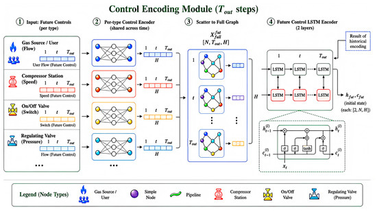
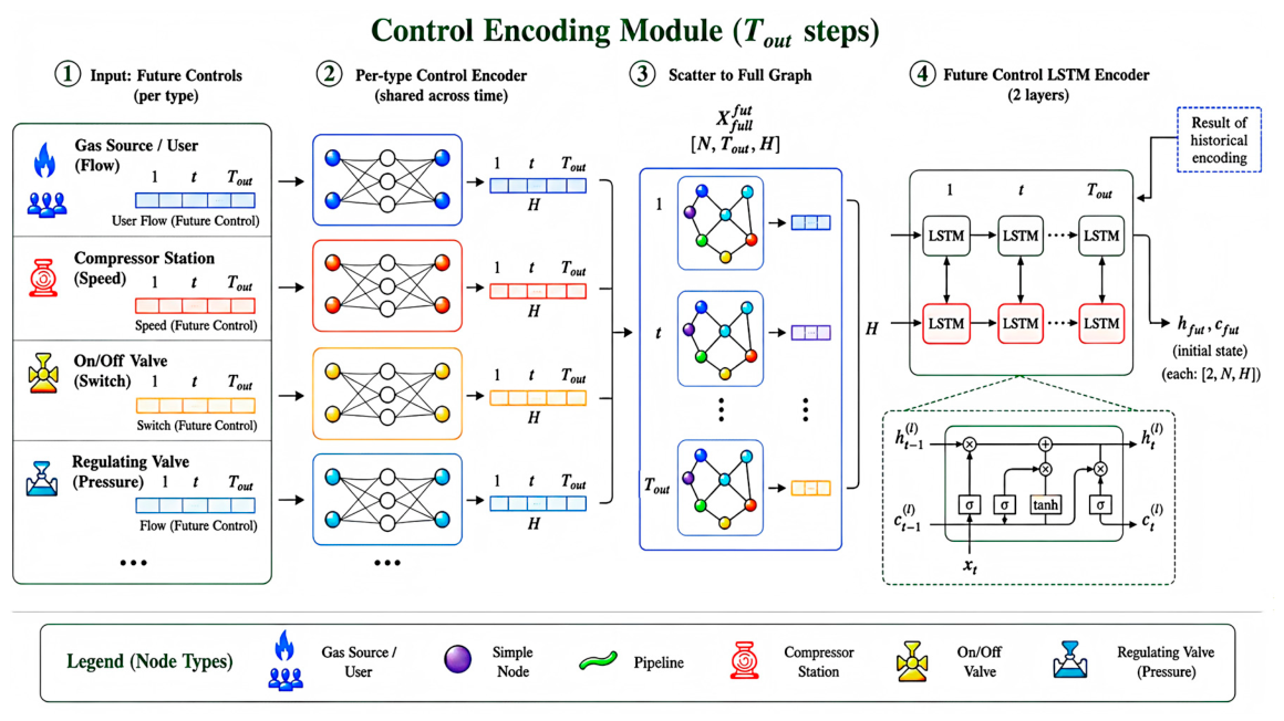
The future-control encoding module extracts the dynamic driving features of external dispatching commands over the prediction horizon. Its structure is shown in Figure 3.

Figure 3. Schematic of the control encoding module.

Unlike historical states, which cover the full network, future controls such as gas-source load variation, compressor speed regulation, and valve switching act only on the controlled-node set ${\mathcal{K}}_{\mathrm{c}}$. Let the future-control input tensor of type-$\mathrm{k}$ controlled nodes be given in Equation (7):

$$U_k^{\mathrm{f}\mathrm{u}\mathrm{t}}\in {\mathbb{R}}^{N_k\times T_{\mathrm{o}\mathrm{u}\mathrm{t}}\times F_k^{\mathrm{c}\mathrm{t}\mathrm{r}\mathrm{l}}},k\in {\mathcal{K}}_c$$

(7)

where ${\mathrm{T}}_{\mathrm{o}\mathrm{u}\mathrm{t}}$ is the prediction length and ${\mathrm{F}}_{\mathrm{k}}^{\mathrm{c}\mathrm{t}\mathrm{r}\mathrm{l}}$ is the feature dimension of the corresponding control variables.

To account for the physical heterogeneity of control variables, a type-specific MLP with parameters shared over time is used to map them into the latent space, thereby unifying feature dimensions while avoiding semantic mixing among physical variables, as shown in Equation (8):

$$Z_k^{\mathrm{c}\mathrm{t}\mathrm{r}\mathrm{l}}={\varphi }_k^{\mathrm{c}\mathrm{t}\mathrm{r}\mathrm{l}}\left(U_k^{\mathrm{f}\mathrm{u}\mathrm{t}}\right),Z_k^{\mathrm{c}\mathrm{t}\mathrm{r}\mathrm{l}}\in {\mathbb{R}}^{N_k\times T_{\mathrm{o}\mathrm{u}\mathrm{t}}\times H}$$

(8)

To align control features with historical memory in the full-graph coordinate system, the index mapping matrix ${\mathrm{S}}_{\mathrm{k}}$ is again used to scatter local control representations back to the complete pipeline-network topology, as shown in Equation (9):

$$U_{\mathrm{f}\mathrm{u}\mathrm{l}\mathrm{l}}^{\mathrm{c}\mathrm{t}\mathrm{r}\mathrm{l}}=\sum _{k\in {\mathcal{K}}_c}{S}_k{Z}_k^{\mathrm{c}\mathrm{t}\mathrm{r}\mathrm{l}},U_{\mathrm{f}\mathrm{u}\mathrm{l}\mathrm{l}}^{\mathrm{c}\mathrm{t}\mathrm{r}\mathrm{l}}\in {\mathbb{R}}^{N\times T_{\mathrm{o}\mathrm{u}\mathrm{t}}\times H}$$

(9)

For uncontrolled nodes without external dispatching commands, the corresponding positions are padded with zero vectors, as shown in Equation (10):

$$U_{\mathrm{f}\mathrm{u}\mathrm{l}\mathrm{l}}^{\mathrm{c}\mathrm{t}\mathrm{r}\mathrm{l}}\left[i,\tau ,:\right]=0,i\notin {\bigcup }_{k\in {\mathcal{K}}_c}{\mathcal{V}}_k$$

(10)

This procedure transforms the control variables into the same latent space and topological graph as the historical variables, providing the basis for subsequent computation.

2.2.3. Dynamic Gated Coupling Mechanism

The future evolution of a pipeline network is not a simple extrapolation of historical operating conditions; it is jointly governed by system-state inertia and external control disturbances. To address the mismatch between historical inputs (${\mathrm{T}}_{\mathrm{i}\mathrm{n}}$) and future controls (${\mathrm{T}}_{\mathrm{o}\mathrm{u}\mathrm{t}}$) in both temporal scale and variable semantics, a dynamic gated coupling architecture inspired by sequence-to-sequence (Seq2Seq) modeling is designed.

First, the historical final state is directly configured as the initial environment of the decoder (i.e., ${\mathrm{h}}_0^{\mathrm{d}\mathrm{e}\mathrm{c}}={\mathrm{h}}^{\mathrm{h}\mathrm{i}\mathrm{s}\mathrm{t}},{\mathrm{c}}_0^{\mathrm{d}\mathrm{e}\mathrm{c}}={\mathrm{c}}^{\mathrm{h}\mathrm{i}\mathrm{s}\mathrm{t}}$) to ensure physical trajectory continuity at the temporal boundary. Meanwhile, the terminal contextual feature of the historical sequence, ${\mathrm{b}}_{\mathrm{i}}$, is replicated along the prediction horizon to construct a baseline tensor representing system inertia, as shown in Equation (11):

$$B_{i,\tau }=b_i,\tau =\mathrm{1,2},\dots \hspace{0.17em},T_{\mathrm{o}\mathrm{u}\mathrm{t}}$$

(11)

Let the corresponding node-level hidden state output by the future-control encoding module be ${\mathrm{C}}_{\mathrm{i},\mathsf{\tau }}^{\mathrm{c}\mathrm{t}\mathrm{r}\mathrm{l}}\in {\mathbb{R}}^{\mathrm{H}}$. To adaptively quantify the corrective effect of dispatching commands on the baseline inertial field, the two features ${\mathrm{q}}_{\mathrm{i},\mathsf{\tau }}=\left[{\mathrm{B}}_{\mathrm{i},\mathsf{\tau }};{\mathrm{C}}_{\mathrm{i},\mathsf{\tau }}^{\mathrm{c}\mathrm{t}\mathrm{r}\mathrm{l}}\right]$ are concatenated, and a nonlinear gating network ${\mathrm{g}}_{\mathsf{\theta }}(\cdot )$ is used to estimate the disturbance intervention intensity ${\mathsf{\Gamma }}_{\mathrm{i},\mathsf{\tau }}$, as shown in Equation (12):

$${\Gamma }_{i,\tau }=\sigma \left(g_{\theta }\left(q_{i,\tau }\right)\right)$$

(12)

Following the residual-learning principle, the fused historical-control tensor is defined as shown in Equation (13):

$$F_{i,\tau }=B_{i,\tau }+{\Gamma }_{i,\tau }\odot C_{i,\tau }^{\mathrm{c}\mathrm{t}\mathrm{r}\mathrm{l}}$$

(13)

This mechanism enables the model to rely on historical inertia ${\mathrm{B}}_{\mathrm{i},\mathsf{\tau }}$ under steady operating conditions, while adaptively increasing the driving weight of external commands ${\mathrm{C}}_{\mathrm{i},\mathsf{\tau }}^{\mathrm{c}\mathrm{t}\mathrm{r}\mathrm{l}}$ under strong-control scenarios such as compressor speed changes or sudden load variations.

To enhance the engineering interpretability of the fusion process, the normalized historical and control contribution ratios at the local-node level are defined as shown in Equations (14) and (15):

$${\overline{\eta }}_{i,\tau }^{\mathrm{h}\mathrm{i}\mathrm{s}\mathrm{t}}={\displaystyle \frac{{\left|B_{i,\tau }\right|}_1}{{\left|B_{i,\tau }\right|}_1+{\left|{\Gamma }_{i,\tau }\odot C_{i,\tau }^{\mathrm{c}\mathrm{t}\mathrm{r}\mathrm{l}}\right|}_1+\epsilon }}$$

(14)

$${\overline{\eta }}_{i,\tau }^{\mathrm{c}\mathrm{t}\mathrm{r}\mathrm{l}}={\displaystyle \frac{{\left|{\Gamma }_{i,\tau }\odot C_{i,\tau }^{\mathrm{c}\mathrm{t}\mathrm{r}\mathrm{l}}\right|}_1}{{\left|B_{i,\tau }\right|}_1+{\left|{\Gamma }_{i,\tau }\odot C_{i,\tau }^{\mathrm{c}\mathrm{t}\mathrm{r}\mathrm{l}}\right|}_1+\epsilon }}$$

(15)

with ${\overline{\mathsf{\eta }}}_{\mathrm{i},\mathsf{\tau }}^{\mathrm{h}\mathrm{i}\mathrm{s}\mathrm{t}}+{\overline{\mathsf{\eta }}}_{\mathrm{i},\mathsf{\tau }}^{\mathrm{c}\mathrm{t}\mathrm{r}\mathrm{l}}\approx 1$. These indicators quantitatively reveal the evolving sensitivity of different pipeline-network regions to dispatching commands.

Finally, the full-graph spatiotemporal fusion tensor $\mathrm{F}\in {\mathbb{R}}^{\mathrm{N}\times {\mathrm{T}}_{\mathrm{o}\mathrm{u}\mathrm{t}}\times \mathrm{H}}$ is passed to a future global decoder network (LSTM) for temporal rollout, as shown in Equation (16):

$$H_{\mathrm{o}\mathrm{u}\mathrm{t}}^{\mathrm{f}\mathrm{u}\mathrm{l}\mathrm{l}}={\mathrm{L}\mathrm{S}\mathrm{T}\mathrm{M}}_{\mathrm{f}\mathrm{u}\mathrm{t}}\left(F;h_0^{\mathrm{d}\mathrm{e}\mathrm{c}},c_0^{\mathrm{d}\mathrm{e}\mathrm{c}}\right),H_{\mathrm{o}\mathrm{u}\mathrm{t}}^{\mathrm{f}\mathrm{u}\mathrm{l}\mathrm{l}}\in {\mathbb{R}}^{N\times T_{\mathrm{o}\mathrm{u}\mathrm{t}}\times H}$$

(16)

The resulting ${\mathrm{H}}_{\mathrm{o}\mathrm{u}\mathrm{t}}^{\mathrm{f}\mathrm{u}\mathrm{l}\mathrm{l}}$ is a network-wide future latent representation that integrates historical inertia, control disturbance, and topological propagation information.

2.2.4. Type-Specific Prediction Decoding

After the full-graph latent representation is obtained, a homogeneous output head would mix the physical dimensions of heterogeneous equipment such as gas sources, pipelines, and compressor units. Therefore, this study designs a dedicated output module that first decodes globally and then separates representations by equipment type.

First, the topological index mapping matrix ${\mathrm{S}}_{\mathrm{k}}$ is used to accurately extract, from the full-graph hidden state, the feature subtensor associated with type-$\mathrm{k}$ objects in the target prediction set ${\mathcal{K}}_{\mathrm{y}}$, as shown in Equation (17):

$$H_k^{\mathrm{f}\mathrm{u}\mathrm{t}}=S_k^{\mathrm{\top }}{H}_{\mathrm{o}\mathrm{u}\mathrm{t}}^{\mathrm{f}\mathrm{u}\mathrm{l}\mathrm{l}},k\in {\mathcal{K}}_y$$

(17)

Because different equipment types, such as gas-storage injection/withdrawal wells and long-distance pipelines, exhibit different dynamic response rates and smoothness over the future prediction window, a dedicated temporal post-processing network is assigned to each output type to further refine equipment-level local evolution patterns, as shown in Equation (18):

$$R_k^{\mathrm{f}\mathrm{u}\mathrm{t}}={\mathrm{L}\mathrm{S}\mathrm{T}\mathrm{M}}_k^{\mathrm{t}\mathrm{y}\mathrm{p}\mathrm{e}}\left(H_k^{\mathrm{f}\mathrm{u}\mathrm{t}}\right)$$

(18)

Finally, the type-specific MLP decoder $\mathrm{p}\mathrm{s}{\mathrm{i}}_{\mathrm{k}}(\cdot )$ projects the representation into the corresponding engineering physical-variable space, such as nodal pressure and pipeline flow, as shown in Equation (19):

$${\widehat{Y}}_k={\psi }_k\left(R_k^{\mathrm{f}\mathrm{u}\mathrm{t}}\right),k\in {\mathcal{K}}_y$$

(19)

The global prediction set is then reconstructed by combining the prediction tensors of all heterogeneous subclasses, as shown in Equation (20):

$${\widehat{\mathcal{Y}}}_{t+1:t+T_{\mathrm{o}\mathrm{u}\mathrm{t}}}=\{{\widehat{Y}}_{k,t+1:t+T_{\mathrm{o}\mathrm{u}\mathrm{t}}}\mid k\in {\mathcal{K}}_y\}$$

(20)

This architecture preserves the topological coupling boundary of the full pipeline network in the latent space while strictly respecting the multivariate physical semantics of heterogeneous engineering objects at the explicit output layer.

2.3. Autoregressive Rolling Training and Multi-Objective Optimization

To overcome exposure bias and long-horizon divergence, which commonly occur in multistep temporal models, this study introduces an autoregressive rolling training paradigm and applies a multi-objective composite constraint that accounts for physical evolution trends. This strategy balances short-term prediction accuracy and long-term stability.

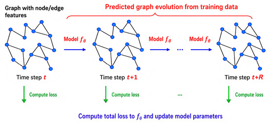
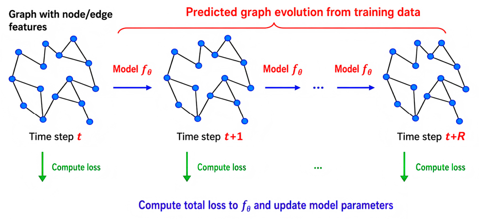
The recursive training procedure is shown in Figure 4. First, the initial historical observation window is set to ${\mathcal{H}}^{\left(0\right)}={\mathcal{X}}_{\mathrm{t}-{\mathrm{T}}_{\mathrm{i}\mathrm{n}}+1:\mathrm{t}}^{\mathrm{h}\mathrm{i}\mathrm{s}\mathrm{t}}$. During the $\mathrm{r}$-th training iteration, the surrogate network outputs the future prediction sequence, as shown in Equation (21):

$${\widehat{\mathcal{Y}}}_{1:T_{\mathrm{o}\mathrm{u}\mathrm{t}}}^{\left(r\right)}=f_{\theta }({\mathcal{H}}^{\left(r\right)},{\mathcal{U}}^{\left(r\right)},\mathcal{G}),r=\mathrm{0,1},\dots \hspace{0.17em},R-1$$

(21)

Figure 4. Schematic of recursive training.

To enable the model to adapt to its own output bias during training, a state-backfilling operator $\mathcal{R}(\cdot )$ is used to reconstruct the historical input for the next window from the previous model prediction rather than from the ground-truth label, as shown in Equation (22):

$${\widehat{\mathcal{X}}}_{\mathrm{n}\mathrm{e}\mathrm{x}\mathrm{t}}^{\left(r\right)}=\mathcal{R}\left({\widehat{\mathcal{Y}}}_1^{\left(r\right)},{\mathcal{U}}_{t+r+1}^{\mathrm{f}\mathrm{u}\mathrm{t}},\mathcal{A}\right)$$

(22)

The autoregressive depth is set to $\mathrm{R}=12$, so that one complete rolling chain spans $6$ h of total prediction time. This design enables the training process to account for cumulative errors induced by recursive prediction. The rolling depth R = 12 is chosen to match the longest dispatching response cycle of interest (a 6 h horizon at the 30 min sampling interval): it must be large enough to expose the network to accumulated self-feedback error, yet not so large that early-step noise dominates training. To justify this choice, an ablation over R in {6, 8, 10, 12} was conducted (Table 1); accuracy improves steadily as R increases and saturates at R = 12, while shorter horizons leave long-term divergence insufficiently constrained, and larger depths bring no further benefit at higher training cost.

Table 1. Ablation of the autoregressive rolling depth R (identical data split and training budget).

Rolling Depth R	Horizon (h)	Pressure Median RE (%)	Flow Median RE (%)
6	3	2.34	4.56
8	4	1.85	3.42
10	5	1.42	2.65
12 (adopted)	6	1.15	2.10

Within each local rolling window, optimizing only pointwise error can lead to numerical oscillations in pressure and flow curves. Therefore, a composite loss function containing both numerical error and temporal-gradient constraints is constructed. For the $\mathrm{r}$-th iteration, the mean squared error term considering node-type weights ${\mathsf{\lambda }}_{\mathrm{k}}$ and variable weights ${\mathsf{\omega }}_{\mathrm{k},\mathrm{m}}$ is defined as shown in Equation (23):

$${\mathcal{L}}_{\mathrm{v}\mathrm{a}\mathrm{l}\mathrm{u}\mathrm{e}}^{\left(r\right)}=\sum _{k\in {\mathcal{K}}_y}{\lambda }_k{\displaystyle \frac{1}{N_k{T}_{\mathrm{o}\mathrm{u}\mathrm{t}}{F}_k^{\mathrm{o}\mathrm{u}\mathrm{t}}}}{\displaystyle \sum _{i=1}^{N_k}}{\displaystyle \sum _{\tau =1}^{T_{\mathrm{o}\mathrm{u}\mathrm{t}}}}{\displaystyle \sum _{m=1}^{F_k^{\mathrm{o}\mathrm{u}\mathrm{t}}}}{\omega }_{k,m}{({\widehat{Y}}_{k,i,\tau ,m}^{\left(r\right)}-Y_{k,i,\tau ,m}^{\left(r\right)})}^2$$

(23)

In addition, the forward difference between adjacent time steps, ${\mathsf{\Delta }}_{\mathsf{\tau }}\mathrm{Y}={\mathrm{Y}}_{\mathsf{\tau }}-{\mathrm{Y}}_{\mathsf{\tau }-1}$, is extracted to construct a temporal-gradient loss that strongly constrains the ramp-up or steep-drop trends of fluid dynamics, as shown in Equation (24):

$${\mathcal{L}}_{\mathrm{v}\mathrm{a}\mathrm{l}\mathrm{u}\mathrm{e}}^{\left(r\right)}=\sum _{k\in {\mathcal{K}}_y}{\lambda }_k{\displaystyle \frac{1}{N_k(T_{\mathrm{o}\mathrm{u}\mathrm{t}}-1)F_k^{\mathrm{o}\mathrm{u}\mathrm{t}}}}{\displaystyle \sum _{i=1}^{N_k}}{\displaystyle \sum _{\tau =1}^{T_{\mathrm{o}\mathrm{u}\mathrm{t}}}}{\displaystyle \sum _{m=1}^{F_k^{\mathrm{o}\mathrm{u}\mathrm{t}}}}{\omega }_{k,m}{[{\Delta }_{\tau }{\widehat{Y}}_{k,i,\tau ,m}^{\left(r\right)}-{\Delta }_{\tau }{Y}_{k,i,\tau ,m}^{\left(r\right)}]}^2$$

(24)

Finally, the entire autoregressive lifecycle is integrated by introducing a global balancing coefficient ${\mathsf{\alpha }}_{\mathrm{v}},{\mathsf{\alpha }}_{\mathrm{g}}$ and a time-decay factor ${\mathsf{\mu }}_{\mathrm{r}}$ that increases with the rolling step, yielding the global expected loss, as shown in Equation (25):

$${\mathcal{L}}_{\mathrm{r}\mathrm{o}\mathrm{l}\mathrm{l}}={\displaystyle \sum _{r=0}^{R-1}}{\mu }_r\left({\alpha }_v{\mathcal{L}}_{\mathrm{v}\mathrm{a}\mathrm{l}\mathrm{u}\mathrm{e}}^{\left(r\right)}+{\alpha }_g{s}_g{\mathcal{L}}_{\mathrm{t}\mathrm{r}\mathrm{e}\mathrm{n}\mathrm{d}}^{\left(r\right)}\right)$$

(25)

The optimal surrogate-model parameters are obtained by minimizing this cumulative expectation, as shown in Equation (26):

$${\theta }^{\mathrm{*}}=\mathrm{a}\mathrm{r}\mathrm{g}\underset{\theta }{\mathrm{m}\mathrm{i}\mathrm{n}}\mathbb{E}\left[{\mathcal{L}}_{\mathrm{r}\mathrm{o}\mathrm{l}\mathrm{l}}\right]$$

(26)

Through the dual design of output self-cycling and hard gradient constraints, this mechanism substantially reduces the risk of prediction divergence under severe dispatching conditions.

3. Model Validation

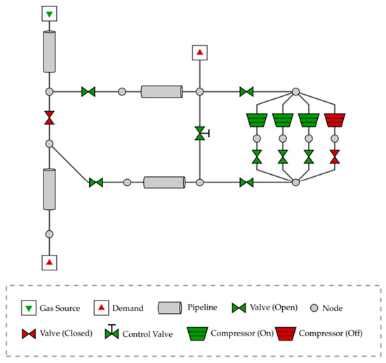
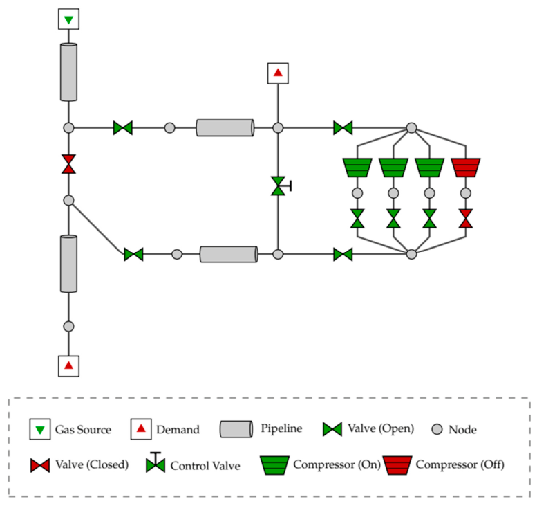
This section validates the proposed method using a mechanistic simulation model of a regional natural gas pipeline network. The network contains 16 flow-controlled gas sources, 7 pressure-controlled gas sources, 507 user nodes, 1079 ordinary valves, 1701 ordinary nodes, 30 flow-regulating valves, 79 compressors, and 752 pipelines. Based on this mechanistic model, quantity and spatial-coordinate information for different component types, including gas sources, users, pipelines, valves, and compressors, is collected and extracted. A unique identifier is assigned to each component to establish a unified component-indexing system and ensure one-to-one correspondence among topology, feature vectors, and prediction outputs. Figure 5 shows a representative local section of the topology, illustrating the principal component types and their connections; the full-network scale is summarized by the statistics above.

Figure 5. Basic composition of the pipeline-network structure.

3.1. Training Data Acquisition and Preprocessing

The dataset used for model training and validation is jointly constructed from actual monitoring data of the natural gas pipeline network and disturbance simulation data generated by the mechanistic model. To address sensor missingness and data-acquisition anomalies commonly observed in real pipeline networks, a real-data reconstruction mechanism based on physical constraints and mechanistic simulation is developed. Specifically, real-time operating information and boundary dispatching commands are first collected from key monitoring points. Pressure or flow nodes with missing values are then interpolated and completed according to fluid-mechanics constraints to ensure complete model inputs. Finally, the completed real boundary conditions are imported into a commercial mechanistic simulation system for full-network state rollout, and the simulated results at monitored nodes are hard-replaced by the corresponding measured values. This mechanism compensates for the spatial sparsity of real data while preserving the physical characteristics of actual operating conditions to the greatest extent possible.

To further enhance model generalization under complex dispatching scenarios, a large-scale simulation dataset based on random disturbances is constructed using historical operating information. The data are generated from typical dispatching conditions and downstream user loads derived from historical real operation. In the case construction process, the input control variables include gas-source pressure/flow setpoints, user load demand, regulating-valve setpoints, valve open/closed states, compressor start/stop states, and compressor outlet pressure. Continuous control variables are augmented by multidimensional perturbations within the neighborhood of historical operating conditions using Latin hypercube sampling, whereas discrete variables are subjected to random 0/1 state switching. To avoid unreasonable or infeasible production schemes, a strict set of engineering constraints is introduced. For example, outlet pressures of parallel compressors in the same station must remain consistent, compressor start/stop states must be strictly coupled with station-bypass or bypass-valve states, and normally open or normally closed valve states are frozen. Only disturbance cases that pass constraint verification are submitted to the mechanistic solver. If simulation diverges or numerical violations occur, the sample is automatically discarded, ensuring the physical consistency and numerical stability of the generated data at the source.

After batch generation of operating cases, a commercial simulation platform is used to perform full-network dynamic solution uniformly. In the simulation settings, the continuous physical operation time of each case is set to 24 h, and boundary dispatching commands are dynamically updated every 3 h to impose external disturbances. Because the surrogate model uses 30 min as the base prediction time step, the transient sequences output by the commercial simulator are further resampled and aligned along the temporal dimension. After strict anomaly removal and spatiotemporal reconstruction, a comprehensive pipeline-network operating dataset containing 85,248 valid time-series samples is obtained, providing complete data support for long-horizon training and generalization testing of the deep spatiotemporal surrogate model.

After data acquisition, the samples are divided into training, validation, and test sets at an 8:1:1 ratio. To prevent temporal and scenario leakage, the split is performed at the level of independent simulation scenarios rather than by randomly shuffling individual time steps: all sliding windows generated from one continuous operating scenario are assigned entirely to a single subset, so that no window in the validation or test set shares time steps with, or originates from the same disturbance realization as, any training window. Within each scenario, the ordering is strictly chronological, and the normalization statistics (for the logarithmic and improved max-min transforms) are estimated on the training set only and then applied unchanged to the validation and test sets. Node features are uniformly mapped to the interval [−1, 1], eliminating dimensional-scale differences and improving network convergence efficiency.

3.2. Model Training

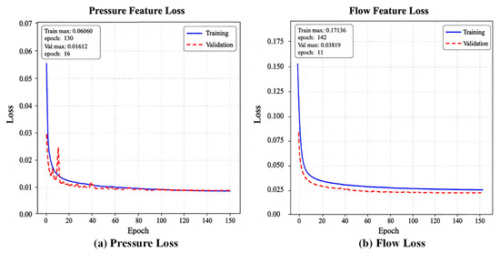
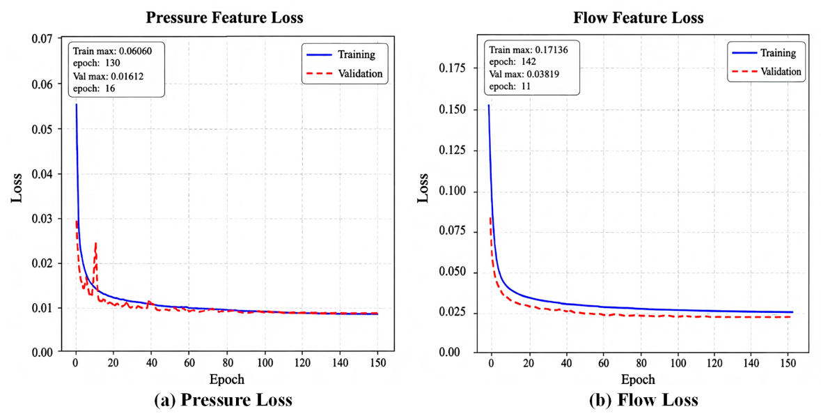
During training, the model is optimized using AdamW with an initial learning rate of 0.001 and a learning-rate decay strategy. The batch size is set to 64. All training is performed on an NVIDIA RTX 5060 Ti GPU with 16 GB memory and lasts approximately 6 h, with the maximum number of epochs set to 150. The results are shown in Figure 6. As training proceeds, both the training and validation losses converge to stable values without obvious oscillation, indicating that the training process has reached convergence. In addition, the converged validation loss is close to the training loss, suggesting that no obvious overfitting occurs.

Figure 6. Training loss curves.

3.3. Single-Case Result Analysis

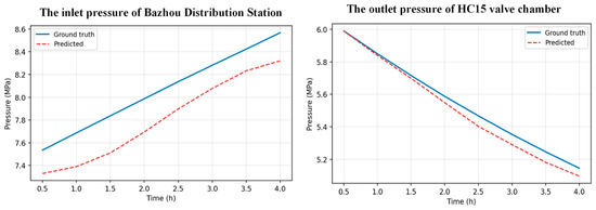
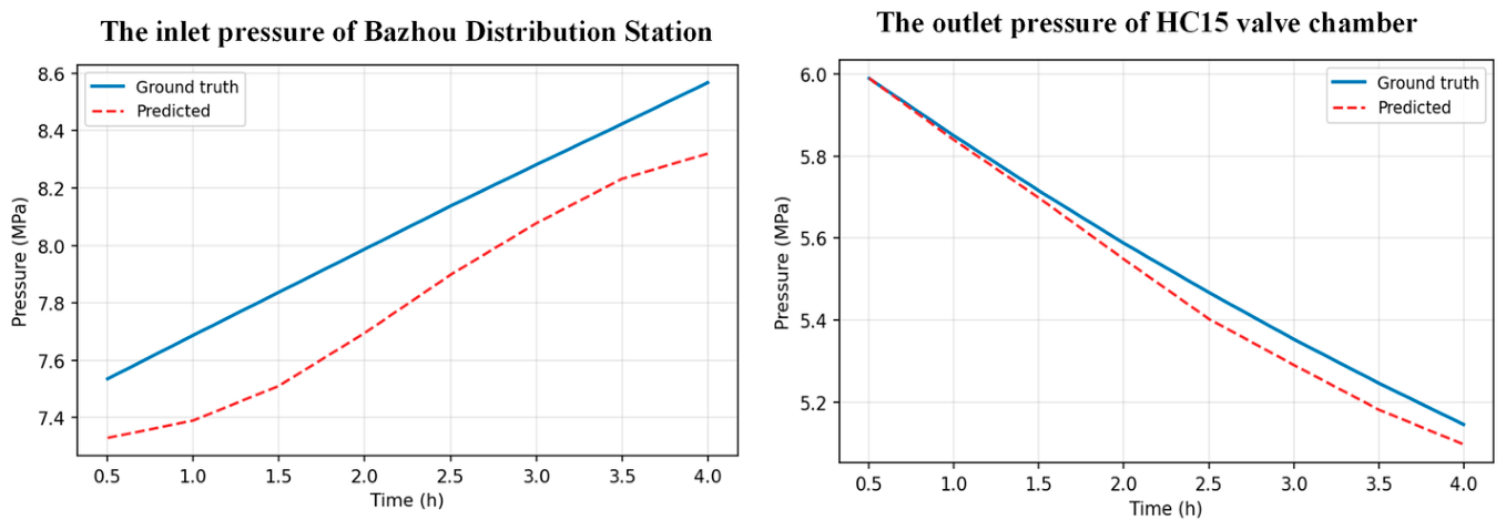
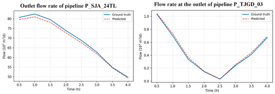
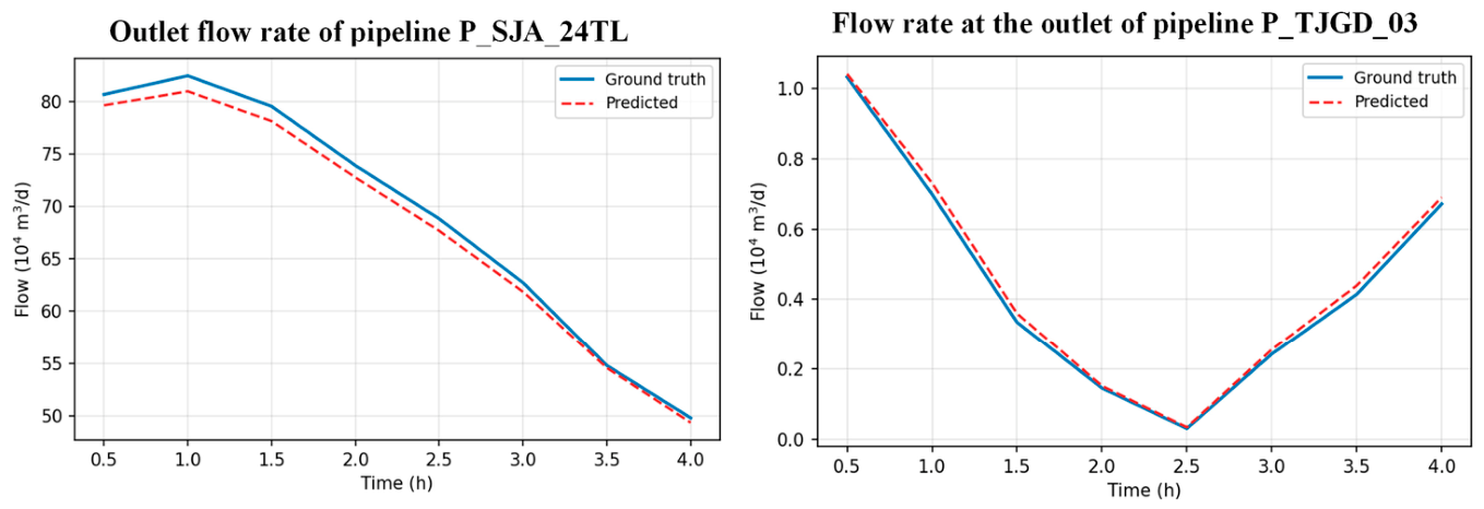
To visually evaluate the physical fidelity of the surrogate model in long-horizon multistep prediction, a typical dynamic dispatching case is randomly selected from the test set. The predicted trajectories of pressure at two representative nodes (Figure 7) and flow in two key pipelines (Figure 8) are compared with mechanistic simulation results. Overall, the model predictions (red dashed lines) agree closely with the mechanistic simulation values (blue solid lines), indicating that the surrogate model accurately captures the dynamic evolution of hydraulic properties over time.

Figure 7. Pressure curves at representative nodes.

Figure 8. Flow-rate curves at representative pipelines.

For nodal-pressure prediction (Figure 7), the two representative nodes exhibit distinct macroscopic evolution patterns. The left panel, corresponding to the inlet pressure of the Bazhou Distribution Station, shows a continuous monotonic increase, whereas the right panel, corresponding to the outlet pressure of the HC15 valve chamber, shows continuous monotonic decay. The surrogate model accurately captures the slopes of these two opposite slowly varying trends. For the Bazhou Distribution Station, although a small initial systematic offset exists between the predicted and true curves, with the predicted values being slightly lower overall, the dynamic increment and curve shape remain highly parallel to the mechanistic simulation result. For the HC15 valve chamber, the predicted curve closely follows the true value over most of the horizon, with only minor cumulative deviation near the end of the prediction window (3.5–4.0 h) due to multistep autoregression. These results show that the model effectively suppresses long-range divergence while accurately representing the inertial evolution of slowly varying state variables such as pressure.

Compared with pressure, which changes relatively smoothly, pipeline flow exhibits stronger nonlinearity and transient behavior because it is more directly driven by external dispatching commands. For pipeline-flow prediction (Figure 8), the two sampled pipelines undergo substantial operating-condition fluctuations during the 4 h prediction window. The left panel, corresponding to the outlet flow of pipeline P_SJA_24TL, first shows a slight increase and then a sustained sharp decline. The right panel, corresponding to the outlet flow of pipeline P_TJGD_03, exhibits a pronounced V-shaped fluctuation: the flow drops abruptly to nearly zero and then rebounds rapidly. Even under such severe operating transitions, the surrogate model maintains high temporal tracking accuracy. At hydraulic turning points such as peaks and troughs, including the 2.5 h point in the right panel, the predicted curves show neither obvious phase delay nor amplitude attenuation, reproducing the transient response details of fluid flow in the complex network topology.

The visual and trend-based analysis of the single case demonstrates that the proposed deep spatiotemporal surrogate model not only accurately fits the macroscopic inertial evolution of pressure, but also sensitively captures high-frequency and abrupt flow variations. These results confirm the robustness and high fidelity of the model architecture for multivariable, strongly nonlinear, and strongly coupled evolution processes in natural gas pipeline networks.

3.4. All-Case Result Analysis

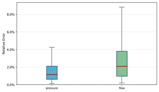
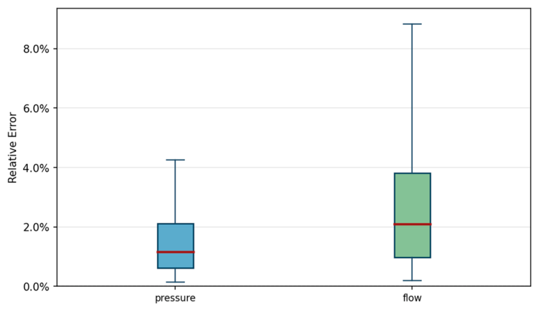
To avoid evaluation bias caused by a single random case, the prediction results for all samples in the test set are further analyzed statistically. Figure 9 shows boxplot distributions of the relative prediction errors for nodal pressure and pipeline flow across all test cases. From the overall statistical results, the surrogate model exhibits excellent generalization capability and prediction accuracy over a large number of heterogeneous test samples.

Figure 9. Boxplot distributions of prediction errors over all test cases.

For nodal-pressure prediction, the median relative error remains approximately 1.15%, and the central distribution interval, namely the interquartile range (IQR), is highly concentrated between 0.60% and 2.10%. In addition, the maximum statistical error boundary for pressure is effectively controlled at approximately 4.20%. These results indicate that the model captures the macroscopic slow-varying characteristics and spatial topological distribution of pipeline-network pressure with high stability. The overall dispersion of the prediction results is very low, demonstrating strong engineering reliability.

Compared with pressure, pipeline flow responds more strongly to external dispatching commands such as compressor start/stop and sudden load changes, and therefore exhibits more pronounced nonlinear transient fluctuations. Consequently, its overall prediction error is slightly higher than that of pressure. The statistics show that the median relative error of flow prediction is 2.10%, the central distribution interval ranges from 1.00% to 3.80%, and the maximum error boundary is approximately 8.80%. Although high-frequency flow transients increase the dispersion of the error distribution, the overall relative error remains within an acceptable engineering range.

3.5. Mechanism Analysis: Dynamic Gating Under Typical Dispatching Events

To make the dynamic gated coupling mechanism interpretable, the normalized control-contribution ratio g defined in Equations (14) and (15) is tracked at representative controlled nodes throughout the prediction horizon. Under steady operation, g remains close to zero and the prediction is dominated by historical inertia, which is consistent with the smooth hydraulic evolution of the network when no new dispatching command is imposed. When a dispatching event occurs, the gate shifts toward the control branch in an event-dependent manner. During compressor start/stop, g increases most evidently at the corresponding compressor station and its first-order topological neighbors, indicating that the model recognizes the compressor command as the dominant driver of the subsequent transient. During valve switching, the increase in g is more localized, marking the abrupt change of the hydraulic boundary near the valve. Under load disturbance, g usually rises more gradually and follows the ramp rate of source or user demand, showing that the model responds to continuously changing external forcing rather than treating it as an instantaneous shock. After the transient response is absorbed by the network, g relaxes toward the history-dominated regime. This behavior indicates that the residual-gated coupling mechanism adaptively re-weights historical inertia and future dispatching controls in a physically consistent manner, thereby providing engineering interpretability for the fusion process without requiring an additional figure.

3.6. Comparison with Baseline Models

To demonstrate the advantage of the proposed method, representative baselines were implemented under identical data splits, feature preprocessing, and training budget, and evaluated on the same test set: (1) a plain LSTM that ignores network topology; (2) a GCN-LSTM that adds spatial graph convolution but uses homogeneous nodes and simple feature concatenation; and (3) an ablated variant of the proposed model without the dynamic gating mechanism. Table 2 reports the median relative errors together with model size and inference time. The proposed model achieves the lowest pressure and flow errors, confirming that the type-specific encoding and residual-gated coupling contribute beyond a generic GCN-LSTM. The statistical spread over all test cases (interquartile range and ±1 standard deviation) is reported in the boxplots of Figure 9, indicating that the improvement is consistent across test cases rather than driven by a few favorable samples.

Table 2. Comparison with baseline models on the same test set (lower is better).

Model	Pressure Median RE (%)	Flow Median RE (%)	Params (M)/Inference Time (ms)
LSTM (no topology)	3.45	6.12	1.8/15
GCN-LSTM (homogeneous)	2.38	4.35	2.6/28
Proposed w/o dynamic gating	1.56	2.84	3.5/40
Proposed (full)	1.15	2.10	4.2/48

3.7. Computational Efficiency and Economic Benefit

Beyond accuracy, the practical value of a surrogate model lies in its computational efficiency. For one 6 h continuous-dispatching scenario, the full-network solution obtained from the commercial mechanistic simulator requires about 240 s, whereas a single forward rollout of the proposed surrogate on the same hardware requires only about 48 ms, i.e., a speed-up of roughly 5000 times. This low-latency inference makes the model suitable for online what-if simulation and real-time early warning, where the mechanistic solver is too slow to be queried repeatedly. From an economic standpoint, the reduced computational cost and the ability to pre-screen dispatching plans help avoid unnecessary compressor energy consumption and curtailment, supporting more economically efficient operation of the pipeline network.

4. Conclusions

This study proposed a deep spatiotemporal surrogate model that jointly addresses topological coupling, equipment heterogeneity, and multistep error accumulation in natural gas pipeline-network state prediction. The verified results are summarized as follows:

(1) To effectively disentangle heterogeneous equipment attributes and fuse historical inertia with future control signals, we propose a shared GCN with type-specific encoding alongside a residual-gated coupling mechanism. Furthermore, a 12-step autoregressive rolling strategy with a temporal-gradient loss is employed to suppress cumulative divergence over the 6 h horizon.

(2) On 85,248 samples from field monitoring data and commercial mechanistic simulations, the median relative errors are 1.15% (nodal pressure) and 2.10% (pipeline flow); the model reproduces macroscopic pressure decay and high-frequency transient flow at valve/compressor switching without obvious phase delay.

(3) Mechanism analysis shows the dynamic gate shifts from history-dominated to control-dominated behavior during compressor switching, valve operation, and load disturbance, supporting engineering interpretability. Future work will couple the surrogate with physics-informed constraints and validate it on abnormal operating states such as line-pack anomalies and leakage.

References

- Economides, M.J.; Wood, D.A. The state of natural gas. J. Nat. Gas Sci. Eng. 2009, 1, 1–13. [Google Scholar] [CrossRef] [Scilit]
- Faramawy, S.; Zaki, T.; Sakr, A.A.E. Natural gas origin, composition, and processing: A review. J. Nat. Gas Sci. Eng. 2016, 34, 34–54. [Google Scholar] [CrossRef] [Scilit]
- Li, J.; Dong, X.; Shangguan, J.; Hook, M. Forecasting the growth of China’s natural gas consumption. Energy 2011, 36, 1380–1385. [Google Scholar] [CrossRef] [Scilit]
- Qian, J.; Han, X.; Ye, M.; Lv, Y.; Che, J. Environmental benefits of the West-East Natural Gas Transmission Project: Cross-regional energy optimization and transformation for sustainable development. Energies 2024, 17, 3820. [Google Scholar] [CrossRef] [Scilit]
- Zhao, Y.; Wang, D. Spatial connection network characteristics and development trend forecast of natural gas industry’s sustainable development resilience in China. Sci. Prog. 2023, 106, 1–25. [Google Scholar] [CrossRef] [Scilit] [PubMed]
- Rios-Mercado, R.Z.; Borraz-Sanchez, C. Optimization problems in natural gas transportation systems: A state-of-the-art review. Appl. Energy 2015, 147, 536–555. [Google Scholar] [CrossRef] [Scilit]
- Su, H.; Zio, E.; Zhang, J.; Li, X.; Chi, L.; Fan, L.; Zhang, Z. A method for the multi-objective optimization of the operation of natural gas pipeline networks considering supply reliability and operation efficiency. Comput. Chem. Eng. 2019, 131, 106584. [Google Scholar] [CrossRef] [Scilit]
- Osiadacz, A.J.; Isoli, N. Multi-objective optimization of gas pipeline networks. Energies 2020, 13, 5141. [Google Scholar] [CrossRef] [Scilit]
- Peng, J.; Zhou, J.; Liang, G.; Li, C.; Qin, C. Multi-period integrated scheduling optimization of complex natural gas pipeline network system with underground gas storage to ensure economic and environmental benefits. Energy 2024, 302, 131837. [Google Scholar] [CrossRef] [Scilit]
- Wei, X.; Qiu, R.; Zhang, B.; Liu, C.; Wang, G.; Wang, B.; Liang, Y. Operation optimization of large-scale natural gas pipeline networks based on intelligent algorithm. Energy 2024, 310, 133258. [Google Scholar] [CrossRef] [Scilit]
- Liu, E.; Lv, L.; Ma, Q.; Kuang, J.; Zhang, L. Steady-state optimization operation of the West-East Gas Pipeline. Adv. Mech. Eng. 2019, 11, 1–14. [Google Scholar] [CrossRef] [Scilit]
- Woldeyohannes, A.D.; Abd Majid, M.A. Simulation model for natural gas transmission pipeline network system. Simul. Model. Pract. Theory 2011, 19, 196–212. [Google Scholar] [CrossRef] [Scilit]
- Herran-Gonzalez, A.; de la Cruz, J.M.; de Andres-Toro, B.; Risco-Martin, J.L. Modeling and simulation of a gas distribution pipeline network. Appl. Math. Model. 2009, 33, 1584–1600. [Google Scholar] [CrossRef] [Scilit]
- Pambour, K.A.; Bolado-Lavin, R.; Dijkema, G.P.J. An integrated transient model for simulating the operation of natural gas transport systems. J. Nat. Gas Sci. Eng. 2016, 28, 672–690. [Google Scholar] [CrossRef] [Scilit]
- Alamian, R.; Behbahani-Nejad, M.; Ghanbarzadeh, A. A state space model for transient flow simulation in natural gas pipelines. J. Nat. Gas Sci. Eng. 2012, 9, 51–59. [Google Scholar] [CrossRef] [Scilit]
- Hochreiter, S.; Schmidhuber, J. Long short-term memory. Neural Comput. 1997, 9, 1735–1780. [Google Scholar] [CrossRef] [Scilit] [PubMed]
- Laib, O.; Khadir, M.T.; Mihaylova, L. Toward efficient energy systems based on natural gas consumption prediction with LSTM recurrent neural networks. Energy 2019, 177, 530–542. [Google Scholar] [CrossRef] [Scilit]
- Liu, L.; Liang, J.; Ma, L.; Zhang, H.; Li, Z.; Liang, S. Gas pipeline flow prediction model based on LSTM with grid search parameter optimization. Processes 2023, 11, 63. [Google Scholar] [CrossRef] [Scilit]
- Sharma, V.; Cali, Ü.; Sardana, B.; Kuzlu, M.; Banga, D.; Pipattanasomporn, M. Data-driven short-term natural gas demand forecasting with machine learning techniques. J. Pet. Sci. Eng. 2021, 206, 108979. [Google Scholar] [CrossRef] [Scilit]
- Yin, X.; Wen, K.; Huang, W.; Luo, Y.; Ding, Y.; Gong, J.; Gao, J.; Hong, B. A high-accuracy online transient simulation framework of natural gas pipeline network by integrating physics-based and data-driven methods. Appl. Energy 2023, 333, 120615. [Google Scholar] [CrossRef] [Scilit]
- Zhou, D.; Jia, X.; Ma, S.; Shao, T.; Huang, D.; Hao, J.; Li, T. Dynamic simulation of natural gas pipeline network based on interpretable machine learning model. Energy 2022, 253, 124068. [Google Scholar] [CrossRef] [Scilit]
- Fakhroleslam, M.; Boozarjomehry, R.B.; Sahlodin, A.M.; Sin, G.; Mansouri, S.S. Dynamic simulation of natural gas transmission pipeline systems through autoregressive neural networks. Ind. Eng. Chem. Res. 2021, 60, 9851–9859. [Google Scholar] [CrossRef] [Scilit]
- Wu, Z.; Pan, S.; Chen, F.; Long, G.; Zhang, C.; Yu, P.S. A comprehensive survey on graph neural networks. IEEE Trans. Neural Netw. Learn. Syst. 2021, 32, 4–24. [Google Scholar] [CrossRef] [Scilit] [PubMed]
- Sarkar, D.; Roy, S.; Malakar, S.; Sarkar, R. A modified GNN architecture with enhanced aggregator and message passing functions. Eng. Appl. Artif. Intell. 2023, 122, 106077. [Google Scholar] [CrossRef] [Scilit]
- Yang, Z.; Liu, Z.; Zhou, J.; Song, C.; Xiang, Q.; He, Q.; Hu, J.; Faber, M.H.; Zio, E.; Li, Z.; et al. A graph neural network (GNN) method for assigning gas calorific values to natural gas pipeline networks. Energy 2023, 278, 127875. [Google Scholar] [CrossRef] [Scilit]
- Wang, C.; Zhou, D.; Wang, X.; Liu, S.; Shao, T.; Shui, C.; Yan, J. Multiscale graph based spatio-temporal graph convolutional network for energy consumption prediction of natural gas transmission process. Energy 2024, 307, 132489. [Google Scholar] [CrossRef] [Scilit]
- Chen, J.; Pan, S.; Peng, W.; Xu, W. Bilinear Spatiotemporal Fusion Network: An efficient approach for traffic flow prediction. Neural Netw. 2025, 187, 107382. [Google Scholar] [CrossRef] [Scilit] [PubMed]
- Lim, B.; Arik, S.O.; Loeff, N.; Pfister, T. Temporal Fusion Transformers for interpretable multi-horizon time series forecasting. Int. J. Forecast. 2021, 37, 1748–1764. [Google Scholar] [CrossRef] [Scilit]
- Su, L.; Zuo, X.; Li, R.; Wang, X.; Zhao, H.; Huang, B. A systematic review for transformer-based long-term series forecasting. Artif. Intell. Rev. 2025, 58, 80. [Google Scholar] [CrossRef] [Scilit]
- Vo, T.; My, L.N.T. A novel approach of multi-channel attention mechanism for long-sequential multivariate time-series prediction problem. Soft Comput. 2025, 29, 629–644. [Google Scholar] [CrossRef] [Scilit]
- Gao, J.; Wang, S.; Chen, R.; Zhang, C.; Zio, E.; Zhang, Y.; Lu, Y. ZSTT: A zero-shot time-series prediction model based on Transformer and its application to hydraulic actuator performance degradation prediction. IEEE/ASME Trans. Mechatron. 2025. early access. [Google Scholar] [CrossRef] [Scilit]
- Ren, D.; Wang, C.; Wei, X.; Zhang, Y.; Han, S.; Xu, W. Harmonizing physical and deep learning modeling: A computationally efficient and interpretable approach for property prediction. Scr. Mater. 2025, 255, 116350. [Google Scholar] [CrossRef] [Scilit]
- Chen, J.; He, Y.; Xiang, Q.; You, H.; Wang, W.; Li, P.; Zhao, Z.; Yang, Z.; Su, H.; Zhang, J. Short-term demand forecasting and supply assurance evaluation for natural gas pipeline networks based on uncertainty quantification and deep learning. Energies 2026, 19, 1101. [Google Scholar] [CrossRef] [Scilit]
- Zhou, X.; Ye, J.; Zhao, S.; Jin, M.; Hou, Z.; Yang, C.; Li, Z.; Wen, Y.; Yuan, X. Noise-robust and sector-aware representation learning for natural gas demand forecasting. Expert Syst. Appl. 2026, 299, 129964. [Google Scholar] [CrossRef] [Scilit]
Disclaimer/Publisher’s Note: The statements, opinions and data contained in all publications are solely those of the individual author(s) and contributor(s) and not of MDPI and/or the editor(s). MDPI and/or the editor(s) disclaim responsibility for any injury to people or property resulting from any ideas, methods, instructions or products referred to in the content. |
© 2026 by the authors. Licensee MDPI, Basel, Switzerland. This article is an open access article distributed under the terms and conditions of the Creative Commons Attribution (CC BY) license.