Interpolating Missing Spatial Data Using Graph Laplacian Eigenbasis

Abstract

This paper addresses the problem of interpolating missing spatial data at the vertices of a connected undirected simple graph. We show that, by exploiting the eigenbasis of the graph Laplacian, all missing values can be reconstructed even from a single observation. This work establishes a novel connection between spatial statistics and spectral graph theory.

1. Introduction

In this paper, we study the problem of recovering missing spatial data at the vertices of an undirected graph. We assume that the graph is connected. Furthermore, it is simple; that is, it has no self-loops or multiple edges. We demonstrate that by leveraging the structure of the graph, all missing values can be reconstructed even when only a single observation is available. Here, exploiting the graph structure specifically means utilizing the eigenbasis of the graph Laplacian. As shown in Yamada (2023) [1], the graph Laplacian eigenvectors can be ordered according to Geary’s c (Geary, 1954 [2]; Cliff and Ord, 1969, 1970, 1973, 1981 [3,4,5,6]), one of the most widely used measures of spatial autocorrelation, which is a spatial extension of the time series autocorrelation measure developed by von Neumann (1941) [7]. This property is central to our approach. In this paper, we establish a novel connection between spatial statistics and spectral graph theory.

We describe the motivation behind the present study. The Hodrick–Prescott (HP) filter (Hodrick and Prescott, 1997 [8]) is a standard method for estimating time trend in econometrics. However, it cannot be directly applied when missing values are present. To overcome this limitation, Yamada (2022) [9] proposed a generalized version of the HP filter, which allows the estimation of the time trend and the simultaneous interpolation of missing values. A key observation is that a time series can be interpreted as data at the vertices of a path graph. This motivates the spatial extension of the method proposed by Yamada (2022) [9], enabling the interpolation of missing spatial values.

The remainder of this paper is organized as follows. Section 2 presents the preliminaries required for the main result. Section 3 states the main result. In particular, it introduces a method for reconstructing missing spatial data using the graph structure. Section 4 provides the proof of the main result. Section 5 illustrates the application of the proposed method to real data. Section 6 concludes the paper. Appendix A provides an additional proof.

2. Preliminaries

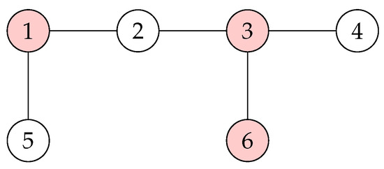
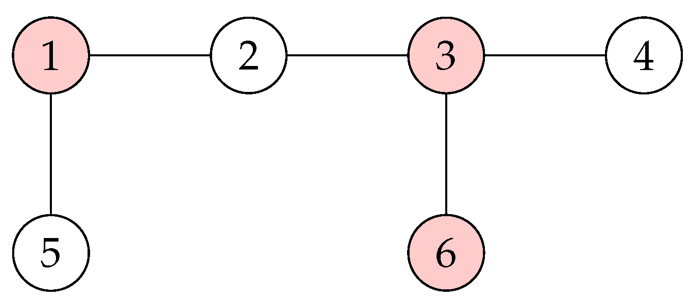
Consider an undirected graph $G=(V,E)$ with no self-loops or multiple edges, where $V=\{1,\dots ,n\}$. We assume that $n=\left|V\right|\ge 2$, $\left|E\right|\ge 1$, and G is connected. Let $A=\{i_1,\dots ,i_m\}$ and $B=\{i_{m+1},\dots ,i_n\}$, where $\{i_1,\dots ,i_n\}=V$ and $1\le m<n$. Then A and B are subsets of the vertex set V such that both A and B are nonempty, $A\cup B=V$, and $A\cap B=\varnothing$. Therefore, $\{A,B\}$ is a partition of V. Let $y_i$ denote the value of y at vertex i for $i=1,\dots ,n$. In this paper, we consider the setting in which $y_i$ is missing for $i\in B$, while $y_i$ is observed for $i\in A$. We refer to the sets A and B as the observed set and the unobserved set, respectively. Figure 1 shows a connected undirected graph with six vertices, where the values at the colored vertices are missing. Accordingly, in this graph, the observed set is $A=\{2,4,5\}$ and the unobserved set is $B=\{1,3,6\}$.

Figure 1. A connected undirected graph. Values at colored vertices are missing.

Let $\mathit{y}={[y_1,\dots ,y_n]}^{\top }$, ${\mathit{y}}_a={[y_{i_1},\dots ,y_{i_m}]}^{\top }$, and ${\mathit{y}}_b={[y_{i_{m+1}},\dots ,y_{i_n}]}^{\top }$. Let ${\mathit{\iota }}_n$ be the n-dimensional column vector of ones, ${\mathit{I}}_n=[{\mathit{e}}_1,\dots ,{\mathit{e}}_n]$ be the identity matrix of order n, and $\mathbf{0}$ denote a zero vector or matrix of appropriate dimension. Let ${\mathit{S}}_a=[{\mathit{e}}_{i_1},\dots ,{\mathit{e}}_{i_m}]$ and ${\mathit{S}}_b=[{\mathit{e}}_{i_{m+1}},\dots ,{\mathit{e}}_{i_n}]$. Then we have ${\mathit{y}}_a={\mathit{S}}_a^{\top }\mathit{y}$ and ${\mathit{y}}_b={\mathit{S}}_b^{\top }\mathit{y}$. Since m is an integer such that $1\le m<n$, both ${\mathit{S}}_a$ and ${\mathit{S}}_b$ are nonzero matrices. Moreover, since $[{\mathit{S}}_a,{\mathit{S}}_b]$ is an $n\times n$ permutation matrix, we have

$$\begin{array}{c}\hfill [{\mathit{S}}_a,{\mathit{S}}_b]\left[\begin{array}{c}{\mathit{S}}_a^{\top }\\ {\mathit{S}}_b^{\top }\end{array}\right]={\mathit{S}}_a{\mathit{S}}_a^{\top }+{\mathit{S}}_b{\mathit{S}}_b^{\top }={\mathit{I}}_n,\end{array}$$

(1)

from which $\mathit{y}$ can be decomposed as

$$\begin{array}{c}\hfill \mathit{y}={\mathit{S}}_a{\mathit{y}}_a+{\mathit{S}}_b{\mathit{y}}_b.\end{array}$$

(2)

Note that ${\mathit{S}}_a{\mathit{y}}_a$ coincides with $\mathit{y}$ on the observed components and is zero on the unobserved components.

Let $\mathit{W}$ be an $n\times n$ matrix whose $(i,j)$ entry is $w_{i,j}$, where

$$\begin{array}{c}\hfill \left\{\begin{array}{cc}{w}_{i,j}>0\hfill & \mathrm{if}\{i,j\}\in E,\hfill \\ w_{i,j}=0\hfill & \mathrm{if}\{i,j\}\notin E,\hfill \end{array}\right.\end{array}$$

(3)

for $i,j=1,\dots ,n$. Since G is an undirected graph with no self-loops or multiple edges, $\mathit{W}$ is a symmetric hollow matrix, i.e., $w_{i,j}=w_{j,i}$ and $w_{i,i}=0$. It is often assumed that $w_{i,j}=1$ whenever $w_{i,j}>0$, in which case $\mathit{W}$ is a binary matrix. Let $\mathit{D}=\mathrm{diag}(d_1,\dots ,d_n)$, where $d_i={\sum }_{j=1}^n{w}_{i,j}$ for $i=1,\dots ,n$. Then the graph Laplacian $\mathit{L}$ corresponding to the graph G can be defined using $\mathit{W}$ and $\mathit{D}$ as

$$\begin{array}{c}\hfill \mathit{L}=\mathit{D}-\mathit{W}.\end{array}$$

(4)

See, e.g., Bapat (2014) [10], Estrada and Knight (2015) [11], and Gallier (2016) [12]. The matrices $\mathit{W}$ and $\mathit{D}$ are referred to as the (weighted) adjacency matrix and the degree matrix of the graph G, respectively.

As an example, we present the graph Laplacian of the graph shown in Figure 1, assuming that the adjacency matrix $\mathit{W}$ is binary. Since the edge set of the graph is

$$\begin{array}{c}\hfill E=\left\{\right\{1,2\},\{1,5\},\{2,3\},\{3,4\},\{3,6\left\}\right\},\end{array}$$

the corresponding graph Laplacian $\mathit{L}$ is given by

$$\begin{array}{ccc}\hfill \mathit{L}& =& \left[\begin{array}{cccccc}2& 0& 0& 0& 0& 0\\ 0& 2& 0& 0& 0& 0\\ 0& 0& 3& 0& 0& 0\\ 0& 0& 0& 1& 0& 0\\ 0& 0& 0& 0& 1& 0\\ 0& 0& 0& 0& 0& 1\end{array}\right]-\left[\begin{array}{cccccc}0& 1& 0& 0& 1& 0\\ 1& 0& 1& 0& 0& 0\\ 0& 1& 0& 1& 0& 1\\ 0& 0& 1& 0& 0& 0\\ 1& 0& 0& 0& 0& 0\\ 0& 0& 1& 0& 0& 0\end{array}\right]\hfill \end{array}$$

(5)

$$\begin{array}{ccc}\hfill & =& \left[\begin{array}{cccccc}2& -1& 0& 0& -1& 0\\ -1& 2& -1& 0& 0& 0\\ 0& -1& 3& -1& 0& -1\\ 0& 0& -1& 1& 0& 0\\ -1& 0& 0& 0& 1& 0\\ 0& 0& -1& 0& 0& 1\end{array}\right].\hspace{1em}\hspace{1em}\hspace{1em}\hspace{1em} \hfill \end{array}$$

(6)

For example, the $(1,2)$ and $(2,1)$ entries of $\mathit{L}$ are −1 since vertices 1 and 2 are adjacent. Similarly, the $(2,2)$ entry is 2 since vertex 2 is adjacent to two other vertices, namely 1 and 3.

We denote the eigenvalues of $\mathit{L}$ by $q_1,\dots ,q_n$ in ascending order. Since the graph G is connected, $\mathit{L}$ has rank $n-1$. Moreover, $\mathit{L}$ is positive semidefinite (see, e.g., Yamada, 2021 [13]). Thus,

$$\begin{array}{c}\hfill q_1=0,0<q_2\le \cdots \le q_n.\end{array}$$

(7)

Let

$$\begin{array}{c}\hfill \mathit{L}=\mathit{P}\mathit{Q}{\mathit{P}}^{\top },\end{array}$$

(8)

be a spectral decomposition of a real symmetric matrix $\mathit{L}$, where $\mathit{Q}=\mathrm{diag}(q_1,\dots ,q_n)$ and $\mathit{P}=[{\mathit{p}}_1,\dots ,{\mathit{p}}_n]$. Then $\mathit{P}$ is an $n\times n$ orthogonal matrix, and hence the column vectors of $\mathit{P}$, $\{{\mathit{p}}_1,\dots ,{\mathit{p}}_n\}$, form an orthonormal basis of ${\mathbb{R}}^n$. In addition, since $\mathit{L}{\mathit{\iota }}_n=\mathbf{0}$, we may take ${\mathit{p}}_1={\displaystyle \frac{1}{\sqrt{n}}}{\mathit{\iota }}_n$, and hence the remaining vectors ${\mathit{p}}_i$ for $i=2,\dots ,n$ lie in the orthogonal complement of $\mathcal{S}\left({\mathit{\iota }}_n\right)$. Here, $\mathcal{S}\left({\mathit{\iota }}_n\right)$ denotes the column space of ${\mathit{\iota }}_n$. Moreover, given that ${\mathit{p}}_i^{\top }\mathit{L}{\mathit{p}}_i=q_i$ for $i=1,\dots ,n$, it follows from (7) that

$$\begin{array}{c}\hfill {\mathit{p}}_1^{\top }\mathit{L}{\mathit{p}}_1=0,0<{\mathit{p}}_2^{\top }\mathit{L}{\mathit{p}}_2\le \cdots \le {\mathit{p}}_n^{\top }\mathit{L}{\mathit{p}}_n.\end{array}$$

(9)

Let $c\left(\mathit{\eta }\right)$ denote the Geary’s c of an n-dimensional column vector $\mathit{\eta }={[{\eta }_1,\dots ,{\eta }_n]}^{\top }\in {\mathbb{R}}^n\setminus \mathcal{S}\left({\mathit{\iota }}_n\right)$ associated with the graph G. Geary’s c is a widely used measure of spatial autocorrelation. As shown in Yamada (2021) [13], it is expressed in terms of ${\mathit{\eta }}^{\top }\mathit{L}\mathit{\eta }$ as

$$\begin{array}{c}\hfill c\left(\mathit{\eta }\right)={\displaystyle \frac{n-1}{{\sum }_{i=1}^n{\sum }_{j=1}^n{w}_{i,j}}}{\displaystyle \frac{\frac{1}{2}{\sum }_{i=1}^n{\sum }_{j=1}^n{w}_{i,j}{({\eta }_i-{\eta }_j)}^2}{{\sum }_{i=1}^n{({\eta }_i-\overline{\eta })}^2}}={\displaystyle \frac{n-1}{{\mathit{\iota }}_n^{\top }\mathit{W}{\mathit{\iota }}_n}}{\displaystyle \frac{{\mathit{\eta }}^{\top }\mathit{L}\mathit{\eta }}{{\mathit{\eta }}^{\top }{\mathit{M}}_n\mathit{\eta }}},\end{array}$$

(10)

where $\overline{\eta }={\displaystyle \frac{1}{n}}{\sum }_{i=1}^n{\eta }_i$ and ${\mathit{M}}_n={\mathit{I}}_n-{\mathit{\iota }}_n{\left({\mathit{\iota }}_n^{\top }{\mathit{\iota }}_n\right)}^{-1}{\mathit{\iota }}_n^{\top }$.

Since ${\mathit{p}}_i$ for $i=2,\dots ,n$ lie in the orthogonal complement of $\mathcal{S}\left({\mathit{\iota }}_n\right)$ and satisfy $\parallel {\mathit{p}}_i\parallel =1$, it follows that ${\mathit{p}}_i^{\top }{\mathit{M}}_n{\mathit{p}}_i={\parallel {\mathit{p}}_i\parallel }^2=1$ for $i=2,\dots ,n$. Thus, Geary’s c for ${\mathit{p}}_i$, $c\left({\mathit{p}}_i\right)$, is given by

$$\begin{array}{c}\hfill c\left({\mathit{p}}_i\right)={\displaystyle \frac{n-1}{{\mathit{\iota }}_n^{\top }\mathit{W}{\mathit{\iota }}_n}}{\mathit{p}}_i^{\top }\mathit{L}{\mathit{p}}_i,\end{array}$$

(11)

for $i=2,\dots ,n$. Therefore, it follows from (9) that

$$\begin{array}{c}\hfill 0<c\left({\mathit{p}}_2\right)\le \cdots \le c\left({\mathit{p}}_n\right).\end{array}$$

(12)

Note that $c\left({\mathit{p}}_1\right)$ is not defined, since ${\mathit{p}}_1^{\top }{\mathit{M}}_n{\mathit{p}}_1=0$.

Equation (12) is crucial for this study. Since Geary’s c takes non-negative values and smaller values indicate stronger positive spatial autocorrelation, the inequalities in (12) imply that, for example, ${\mathit{p}}_i$ exhibits stronger positive spatial autocorrelation in the sense of Geary’s c than ${\mathit{p}}_{i+1}$ for $i=2,\dots ,n-1$.

3. Interpolating Missing Spatial Data

Motivated by the monotonicity condition on the graph Laplacian eigenvectors in (12), we consider the following minimization problem for reconstructing ${\mathit{y}}_b\in {\mathbb{R}}^{n-m}$ from ${\mathit{y}}_a\in {\mathbb{R}}^m$:

$$\begin{array}{c}\underset{{\mathit{y}}_b\in {\mathbb{R}}^{n-m},{\theta }_1,\dots ,{\theta }_n\in \mathbb{R}}{\min }{\parallel ({\mathit{S}}_a{\mathit{y}}_a+{\mathit{S}}_b{\mathit{y}}_b)-({\theta }_1{\mathit{p}}_1+{\theta }_2{\mathit{p}}_2+\cdots +{\theta }_n{\mathit{p}}_n)\parallel }^2,\end{array}$$

(13)

$$\begin{array}{c}\mathrm{s}.\mathrm{t}.q_1{\theta }_1^2+\cdots +q_n{\theta }_n^2\le \kappa ,\end{array}$$

(14)

where $\kappa$ is a positive constant. Note that since $q_1=0$, $q_1{\theta }_1^2+\cdots +q_n{\theta }_n^2$ in the constraint can equivalently be written as $q_2{\theta }_2^2+\cdots +q_n{\theta }_n^2$. Given the ordering condition in (7), the weight associated with ${\theta }_{i+1}$ is greater than or equal to that associated with ${\theta }_i$ for $i=2,\dots ,n-1$. Consequently, under the monotonicity condition on the graph Laplacian eigenvectors in (12), this weighting structure allows for the reconstruction of ${\mathit{y}}_b$.

Let $\mathit{\theta }={[{\theta }_1,\dots ,{\theta }_n]}^{\top }$. Then the above constrained minimization problem can be written in matrix form as

$$\begin{array}{c}\underset{{\mathit{y}}_b\in {\mathbb{R}}^{n-m},\mathit{\theta }\in {\mathbb{R}}^n}{\min }{\parallel ({\mathit{S}}_a{\mathit{y}}_a+{\mathit{S}}_b{\mathit{y}}_b)-\mathit{P}\mathit{\theta }\parallel }^2,\end{array}$$

(15)

$$\begin{array}{c}\mathrm{s}.\mathrm{t}.{\mathit{\theta }}^{\top }\mathit{Q}\mathit{\theta }\le \kappa .\end{array}$$

(16)

Recall that $\mathit{P}=[{\mathit{p}}_1,\dots ,{\mathit{p}}_n]$ and $\mathit{Q}=\mathrm{diag}(q_1,\dots ,q_n)$. The constrained minimization problem (15) and (16) is equivalent to the following penalized least squares problem:

$$\begin{array}{c}\hfill \underset{{\mathit{y}}_b\in {\mathbb{R}}^{n-m},\mathit{\theta }\in {\mathbb{R}}^n}{\min }f({\mathit{y}}_b,\mathit{\theta })={\parallel ({\mathit{S}}_a{\mathit{y}}_a+{\mathit{S}}_b{\mathit{y}}_b)-\mathit{P}\mathit{\theta }\parallel }^2+\lambda {\mathit{\theta }}^{\top }\mathit{Q}\mathit{\theta },\end{array}$$

(17)

where $\lambda$ is a non-negative smoothing parameter. More precisely, for any $\kappa$, there exists a $\lambda$ that yields an equivalent solution (see, e.g., Beck, 2014 [14]). The two parameters, $\kappa$ and $\lambda$, are inversely related. For example, $\kappa \to 0^{+}$ corresponds to $\lambda \to \infty$.

Incidentally, the above penalized least squares problem is similar to that considered in Yamada (2022) [9]. This is because, by letting $\mathit{x}=\mathit{P}\mathit{\theta }$, (17) can be rewritten as a graph Laplacian-penalized least squares problem:

$$\begin{array}{c}\hfill \underset{{\mathit{y}}_b\in {\mathbb{R}}^{n-m},\mathit{x}\in {\mathbb{R}}^n}{\min }g({\mathit{y}}_b,\mathit{x})={\parallel ({\mathit{S}}_a{\mathit{y}}_a+{\mathit{S}}_b{\mathit{y}}_b)-\mathit{x}\parallel }^2+\lambda {\mathit{x}}^{\top }\mathit{L}\mathit{x}.\end{array}$$

(18)

Note that this formulation is equivalent to the spatial smoothing method considered in Yamada (2024) [15] when $m=n$, i.e., when there are no missing values, although this case is not considered in the present paper.

Concerning the minimization problem in (17), the following result holds.

Theorem 1.

If $m\ge 1$ and $\lambda >0$, then there exists a unique global minimizer $({\widehat{\mathit{y}}}_b,\widehat{\mathit{\theta }})$ such that

$$\begin{array}{c}\hfill f({\mathit{y}}_b,\mathit{\theta })\ge f({\widehat{\mathit{y}}}_b,\widehat{\mathit{\theta }}),{\mathit{y}}_b\in {\mathbb{R}}^{n-m},\mathit{\theta }\in {\mathbb{R}}^n,\end{array}$$

(19)

with equality if and only if ${\mathit{y}}_b={\widehat{\mathit{y}}}_b$ and $\mathit{\theta }=\widehat{\mathit{\theta }}$. Moreover, the minimizers are explicitly given by

$$\begin{array}{c}{\widehat{\mathit{y}}}_b={\mathit{S}}_b^{\top }\mathbf{P}\widehat{\mathit{\theta }},\end{array}$$

(20)

$$\begin{array}{c}\widehat{\mathit{\theta }}={\mathbf{P}}^{\top }{({\mathit{S}}_a{\mathit{S}}_a^{\top }+\lambda \mathit{L})}^{-1}{\mathit{S}}_a{\mathit{y}}_a.\end{array}$$

(21)

Proof. 

A proof is given in Section 4.    □

Equation (20) shows that ${\mathit{y}}_b$ can be interpolated using the graph Laplacian eigenbasis $\{{\mathit{p}}_1,\dots ,{\mathit{p}}_n\}$ as

$$\begin{array}{c}\hfill {\widehat{\mathit{y}}}_b={\mathit{S}}_b^{\top }({\widehat{\theta }}_1{\mathit{p}}_1+\cdots +{\widehat{\theta }}_n{\mathit{p}}_n),\end{array}$$

(22)

where ${\widehat{\theta }}_i$ denotes the i-th entry of $\widehat{\mathit{\theta }}$ for $i=1,\dots ,n$. Furthermore, by substituting (21) into (20), we obtain the following alternative representation:

$$\begin{array}{c}\hfill {\widehat{\mathit{y}}}_b={\mathit{S}}_b^{\top }{({\mathit{S}}_a{\mathit{S}}_a^{\top }+\lambda \mathit{L})}^{-1}{\mathit{S}}_a{\mathit{y}}_a,\end{array}$$

(23)

which explicitly shows how ${\widehat{\mathit{y}}}_b$ is reconstructed from the observed data ${\mathit{y}}_a$. Recall that ${\mathit{S}}_a{\mathit{y}}_a$ coincides with $\mathit{y}$ on the observed components and is zero on the unobserved components.

Finally, we make three remarks on the above result. First, ${\mathit{S}}_a{\mathit{S}}_a^{\top }+\lambda \mathit{L}$ is nonsingular because the following lemma holds.

Lemma 1.

If $m\ge 1$, then ${\mathit{S}}_a{\mathit{S}}_a^{\top }+\lambda \mathit{L}$ is positive definite for any positive λ.

Proof. 

First, consider the case where $\mathit{\xi }\in \mathcal{S}\left({\mathit{p}}_1\right)\setminus \left\{\mathbf{0}\right\}$. In this case, $\mathit{\xi }$ can be expressed as $\mathit{\xi }={\mathit{p}}_1\alpha$ for some $\alpha \ne 0$. Since ${\mathit{S}}_a^{\top }{\mathit{p}}_1={\mathit{S}}_a^{\top }({\displaystyle \frac{1}{\sqrt{n}}}{\mathit{\iota }}_n)={\displaystyle \frac{1}{\sqrt{n}}}{\mathit{\iota }}_m$ and $\mathit{L}\mathit{\xi }=\mathit{L}{\mathit{p}}_1\alpha ={\displaystyle \frac{\alpha }{\sqrt{n}}}\mathit{L}{\mathit{\iota }}_n=\mathbf{0}$, we obtain

$$\begin{array}{c}\hfill {\mathit{\xi }}^{\top }({\mathit{S}}_a{\mathit{S}}_a^{\top }+\lambda \mathit{L})\mathit{\xi }={\alpha }^2{\parallel {\mathit{S}}_a^{\top }{\mathit{p}}_1\parallel }^2={\alpha }^2{\displaystyle \frac{m}{n}}>0,\end{array}$$

(24)

if $m\ge 1$.

Next, consider the case where $\mathit{\xi }\in {\mathbb{R}}^n\setminus \mathcal{S}\left({\mathit{p}}_1\right)$. In this case, $\mathit{\xi }$ can be expressed as $\mathit{\xi }={\mathit{p}}_1\alpha +{\mathit{P}}_2\mathit{\beta }$ for some $\alpha$ and some $\mathit{\beta }\ne \mathbf{0}$, where ${\mathit{P}}_2=[{\mathit{p}}_2,\dots ,{\mathit{p}}_n]$. Again, since $\mathit{L}{\mathit{p}}_1=\mathbf{0}$, it follows that

$$\begin{array}{c}\hfill {\mathit{\xi }}^{\top }\mathit{L}\mathit{\xi }={({\mathit{p}}_1\alpha +{\mathit{P}}_2\mathit{\beta })}^{\top }\mathit{L}({\mathit{p}}_1\alpha +{\mathit{P}}_2\mathit{\beta })={\mathit{\beta }}^{\top }{\mathit{P}}_2^{\top }\mathit{P}\mathit{Q}{\mathit{P}}^{\top }{\mathit{P}}_2\mathit{\beta }={\mathit{\beta }}^{\top }{\mathit{Q}}_2\mathit{\beta }>0,\end{array}$$

(25)

where ${\mathit{Q}}_2=\mathrm{diag}(q_2,\dots ,q_n)$. The last inequality follows since ${\mathit{Q}}_2$ is positive definite. Therefore, for any $\lambda >0$, it follows from (25) that

$$\begin{array}{c}\hfill {\mathit{\xi }}^{\top }({\mathit{S}}_a{\mathit{S}}_a^{\top }+\lambda \mathit{L})\mathit{\xi }={\parallel {\mathit{S}}_a^{\top }\mathit{\xi }\parallel }^2+\lambda {\mathit{\xi }}^{\top }\mathit{L}\mathit{\xi }>0.\end{array}$$

(26)

Combining the above cases, we conclude that for any $\mathit{\xi }\in {\mathbb{R}}^n\setminus \left\{\mathbf{0}\right\}$, ${\mathit{\xi }}^{\top }({\mathit{S}}_a{\mathit{S}}_a^{\top }+\lambda \mathit{L})\mathit{\xi }>0$.    □

Accordingly, we note that our main result in (22) requires the condition $m\ge 1$, i.e., at least one data point must be observed.

Second, we show that $\widehat{\mathit{\theta }}$ can be regarded as the solution of a generalized ridge regression (Hoerl and Kennard, 1970 [16]). Let $\mathit{U}={\mathit{S}}_a^{\top }\mathit{P}\in {\mathbb{R}}^{m\times n}$. Then it follows from (21) that

$$\begin{array}{cc}\hfill \widehat{\mathit{\theta }}& ={\mathit{P}}^{\top }{({\mathit{S}}_a{\mathit{S}}_a^{\top }+\lambda \mathit{L})}^{-1}{\mathit{S}}_a{\mathit{y}}_a={\mathit{P}}^{\top }{(\mathit{P}{\mathit{P}}^{\top }{\mathit{S}}_a{\mathit{S}}_a^{\top }\mathit{P}{\mathit{P}}^{\top }+\lambda \mathit{P}\mathit{Q}{\mathbf{P}}^{\top })}^{-1}{\mathit{S}}_a{\mathit{y}}_a\hfill \\ \hfill & ={({\mathit{P}}^{\top }{\mathit{S}}_a{\mathit{S}}_a^{\top }\mathit{P}+\lambda \mathit{Q})}^{-1}{\mathit{P}}^{\top }{\mathit{S}}_a{\mathit{y}}_a={({\mathit{U}}^{\top }\mathit{U}+\lambda \mathit{Q})}^{-1}{\mathit{U}}^{\top }{\mathit{y}}_a,\hfill \end{array}$$

(27)

which is the solution of the following generalized ridge regression:

$$\begin{array}{c}\hfill \underset{\mathit{\theta }\in {\mathbb{R}}^n}{\min }{\parallel {\mathit{y}}_a-\mathit{U}\mathit{\theta }\parallel }^2+\lambda {\mathit{\theta }}^{\top }\mathit{Q}\mathit{\theta }.\end{array}$$

(28)

We note that, even though $\mathit{U}$ is an $m\times n$ matrix with $m<n$, ${\mathit{U}}^{\top }\mathit{U}+\lambda \mathit{Q}$ is positive definite. This follows from the fact that ${\mathit{U}}^{\top }\mathit{U}+\lambda \mathit{Q}$ is similar to ${\mathit{S}}_a{\mathit{S}}_a^{\top }+\lambda \mathit{L}$ as

$$\begin{array}{c}\hfill {\mathbf{P}}^{\top }({\mathit{S}}_a{\mathit{S}}_a^{\top }+\lambda \mathit{L})\mathit{P}={\mathit{P}}^{\top }{\mathit{S}}_a{\mathit{S}}_a^{\top }\mathit{P}+\lambda {\mathit{P}}^{\top }\mathit{L}\mathit{P}={\mathit{U}}^{\top }\mathit{U}+\lambda \mathit{Q}.\end{array}$$

(29)

Third, we provide insights into how ${\widehat{\mathit{y}}}_b$ in (20) depends on the smoothing parameter $\lambda$. In particular, we have

$$\begin{array}{c}\hfill {\widehat{\mathit{y}}}_b\to {\overline{y}}_a{\mathit{\iota }}_{n-m},(\lambda \to \infty ),\end{array}$$

(30)

where ${\overline{y}}_a$ denotes the mean of the entries of ${\mathit{y}}_a$, i.e., ${\overline{y}}_a={\displaystyle \frac{1}{m}}{\sum }_{h=1}^m{y}_{i_h}$. A proof of (30) is given in Appendix A. Furthermore, from Lemma 1, ${\mathit{S}}_a{\mathit{S}}_a^{\top }+\lambda \mathit{L}$ is positive definite for any $\lambda >0$ when $m\ge 1$. However, it becomes ill-conditioned as $\lambda \to 0^{+}$ since ${\mathit{S}}_a{\mathit{S}}_a^{\top }$ is rank-deficient. Therefore, $\lambda$ should not be chosen too small.

4. Proof of Theorem 1

In this section, we provide a proof of Theorem 1.

Proof of Theorem 1.

Let $\mathit{R}=[\mathit{P},-{\mathit{S}}_b]\in {\mathbb{R}}^{n\times (2n-m)}$, $\mathit{\varphi }={[{\mathit{\theta }}^{\top },{\mathit{y}}_b^{\top }]}^{\top }\in {\mathbb{R}}^{2n-m}$, and $\mathbf{\Omega }=\mathrm{diag}(\mathit{Q},\mathbf{0})\in {\mathbb{R}}^{(2n-m)\times (2n-m)}$. Then since

$$\begin{array}{c}({\mathit{S}}_a{\mathit{y}}_a+{\mathit{S}}_b{\mathit{y}}_b)-\mathit{P}\mathit{\theta }={\mathit{S}}_a{\mathit{y}}_a-[\mathit{P},-{\mathit{S}}_b]\left[\begin{array}{c}\mathit{\theta }\\ {\mathit{y}}_b\end{array}\right]={\mathit{S}}_a{\mathit{y}}_a-\mathit{R}\mathit{\varphi },\\ {\mathit{\theta }}^{\top }\mathit{Q}\mathit{\theta }=[{\mathit{\theta }}^{\top },{\mathit{y}}_b^{\top }]\left[\begin{array}{cc}\mathit{Q}& \mathbf{0}\\ \mathbf{0}& \mathbf{0}\end{array}\right]\left[\begin{array}{c}\mathit{\theta }\\ {\mathit{y}}_b\end{array}\right]={\mathit{\varphi }}^{\top }\mathbf{\Omega }\mathit{\varphi },\end{array}$$

the objective function in (17) can be rewritten as

$$\begin{array}{cc}\hfill f\left(\mathit{\varphi }\right)& = \parallel {\mathit{S}}_a{\mathit{y}}_a{-\mathit{R}\mathit{\varphi }\parallel }^2+\lambda {\mathit{\varphi }}^{\top }\mathbf{\Omega }\mathit{\varphi }\hfill \\ \hfill & ={\mathit{\varphi }}^{\top }({\mathit{R}}^{\top }\mathit{R}+\lambda \mathbf{\Omega })\mathit{\varphi }-2{\left({\mathit{S}}_a{\mathit{y}}_a\right)}^{\top }\mathit{R}\mathit{\varphi }+{\left({\mathit{S}}_a{\mathit{y}}_a\right)}^{\top }\left({\mathit{S}}_a{\mathit{y}}_a\right).\hfill \end{array}$$

   □

Accordingly, the Hessian matrix of $f\left(\mathit{\varphi }\right)$ is

$$\begin{array}{c}\hfill \mathit{H}=2({\mathit{R}}^{\top }\mathit{R}+\lambda \mathbf{\Omega })=2\left(\left[\begin{array}{c}{\mathit{P}}^{\top }\\ -{\mathit{S}}_b^{\top }\end{array}\right][\mathit{P},-{\mathit{S}}_b]+\lambda \left[\begin{array}{cc}\mathit{Q}& \mathbf{0}\\ \mathbf{0}& \mathbf{0}\end{array}\right]\right)=2\left[\begin{array}{cc}{\mathit{I}}_n+\lambda \mathit{Q}& -{\mathit{P}}^{\top }{\mathit{S}}_b\\ -{\mathit{S}}_b^{\top }\mathit{P}& {\mathit{I}}_{n-m}\end{array}\right].\end{array}$$

Lemma 2.

If $m\ge 1$, then $\mathit{H}$ is positive definite for any positive λ.

Proof. 

Since both ${\mathit{R}}^{\top }\mathit{R}$ and $\mathbf{\Omega }$ are positive semidefinite and $\lambda >0$, $\mathit{H}$ is positive semidefinite. Then $\mathit{H}$ is positive definite if $\left|\mathit{H}\right|>0$. Since ${\mathit{I}}_n-{\mathit{S}}_b{\mathit{S}}_b^{\top }={\mathit{S}}_a{\mathit{S}}_a^{\top }$ and $\mathit{P}$ is orthogonal, we have

$$\begin{array}{cc}\hfill \left|{\displaystyle \frac{1}{2}}\mathit{H}\right|& =\left|\begin{array}{cc}{\mathit{I}}_n+\lambda \mathit{Q}& -{\mathit{P}}^{\top }{\mathit{S}}_b\\ -{\mathit{S}}_b^{\top }\mathit{P}& {\mathit{I}}_{n-m}\end{array}\right|=|{\mathit{I}}_n+\lambda \mathit{Q}-{\mathit{P}}^{\top }{\mathit{S}}_b{\mathit{S}}_b^{\top }\mathit{P}|\hfill \\ \hfill & =\left|{\mathit{P}}^{\top }({\mathit{I}}_n+\lambda \mathit{P}\mathit{Q}{\mathit{P}}^{\top }-{\mathit{S}}_b{\mathit{S}}_b^{\top })\mathit{P}\right|=\left|{\mathit{P}}^{\top }\right||{\mathit{S}}_a{\mathit{S}}_a^{\top }+\lambda \mathit{L}|\left|\mathit{P}\right|\hfill \\ \hfill & =|{\mathit{S}}_a{\mathit{S}}_a^{\top }+\lambda \mathit{L}|>0,\hfill \end{array}$$

where the last inequality follows from Lemma 1. (Note that ${\mathit{I}}_n+\lambda \mathit{Q}-{\mathit{P}}^{\top }{\mathit{S}}_b{\mathit{S}}_b^{\top }\mathit{P}$ is the Schur complement of ${\mathit{I}}_{n-m}$ in ${\displaystyle \frac{1}{2}}\mathit{H}$.) Therefore, $\left|\mathit{H}\right|>0$. Since $\mathit{H}$ is positive semidefinite, this implies that $\mathit{H}$ is positive definite.

Let $\widehat{\mathit{\varphi }}$ be the column vector such that ${\displaystyle \frac{\partial f(\widehat{\mathit{\varphi }})}{\partial \mathit{\varphi }}}=\mathbf{0}$. Then since $f\left(\mathit{\varphi }\right)$ is quadratic and its Hessian matrix is positive definite from Lemma 2, it follows that

$$\begin{array}{c}\hfill f\left(\mathit{\varphi }\right)-f\left(\widehat{\mathit{\varphi }}\right)={\displaystyle \frac{1}{2}}{(\mathit{\varphi }-\widehat{\mathit{\varphi }})}^{\top }\mathit{H}(\mathit{\varphi }-\widehat{\mathit{\varphi }})>0,\mathit{\varphi }\in {\mathbb{R}}^{2n-m}\setminus \left\{\widehat{\mathit{\varphi }}\right\}.\end{array}$$

Hence, $\widehat{\mathit{\varphi }}$ is the unique global minimizer of $f\left(\mathit{\varphi }\right)$.

Here, since ${\displaystyle \frac{\partial f\left(\mathit{\varphi }\right)}{\partial \mathit{\varphi }}}=2({\mathit{R}}^{\top }\mathit{R}+\lambda \mathbf{\Omega })\mathit{\varphi }-2{\mathit{R}}^{\top }{\mathit{S}}_a{\mathit{y}}_a$, the minimizer $\widehat{\mathit{\varphi }}$ satisfies

$$\begin{array}{c}\hfill ({\mathit{R}}^{\top }\mathit{R}+\lambda \mathbf{\Omega })\widehat{\mathit{\varphi }}={\mathit{R}}^{\top }{\mathit{S}}_a{\mathit{y}}_a.\end{array}$$

(31)

Then given that ${\mathit{S}}_b^{\top }{\mathit{S}}_a{\mathit{y}}_a=\mathbf{0}$, (31) can be written in terms of $\widehat{\mathit{\theta }}$ and ${\widehat{\mathit{y}}}_b$ as

$$\begin{array}{c}\hfill \left[\begin{array}{cc}{\mathit{I}}_n+\lambda \mathit{Q}& -{\mathit{P}}^{\top }{\mathit{S}}_b\\ -{\mathit{S}}_b^{\top }\mathit{P}& {\mathit{I}}_{n-m}\end{array}\right]\left[\begin{array}{c}\widehat{\mathit{\theta }}\\ {\widehat{\mathit{y}}}_b\end{array}\right]=\left[\begin{array}{c}{\mathit{P}}^{\top }{\mathit{S}}_a{\mathit{y}}_a\\ \mathbf{0}\end{array}\right],\end{array}$$

which yields the following system of equations

$$\begin{array}{c}({\mathit{I}}_n+\lambda \mathit{Q})\widehat{\mathit{\theta }}-{\mathit{P}}^{\top }{\mathit{S}}_b{\widehat{\mathit{y}}}_b={\mathit{P}}^{\top }{\mathit{S}}_a{\mathit{y}}_a,\end{array}$$

(32)

$$\begin{array}{c}{\widehat{\mathit{y}}}_b={\mathit{S}}_b^{\top }\mathit{P}\widehat{\mathit{\theta }}.\end{array}$$

(33)

Substituting (33) into (32), we obtain

$$\begin{array}{cc}\hfill ({\mathit{I}}_n+\lambda \mathit{Q})\widehat{\mathit{\theta }}-{\mathit{P}}^{\top }{\mathit{S}}_b{\widehat{\mathit{y}}}_b& =({\mathit{I}}_n+\lambda \mathit{Q})\widehat{\mathit{\theta }}-{\mathit{P}}^{\top }{\mathit{S}}_b{\mathit{S}}_b^{\top }\mathit{P}\widehat{\mathit{\theta }}=({\mathit{I}}_n+\lambda \mathit{Q}-{\mathit{P}}^{\top }{\mathit{S}}_b{\mathit{S}}_b^{\top }\mathit{P})\widehat{\mathit{\theta }}\hfill \\ \hfill & ={\mathit{P}}^{\top }({\mathit{I}}_n+\lambda \mathit{L}-{\mathit{S}}_b{\mathit{S}}_b^{\top })\mathit{P}\widehat{\mathit{\theta }}={\mathit{P}}^{\top }({\mathit{S}}_a{\mathit{S}}_a^{\top }+\lambda \mathit{L})\mathit{P}\widehat{\mathit{\theta }}.\hfill \end{array}$$

Accordingly, (32) becomes

$$\begin{array}{c}\hfill {\mathit{P}}^{\top }({\mathit{S}}_a{\mathit{S}}_a^{\top }+\lambda \mathit{L})\mathit{P}\widehat{\mathit{\theta }}={\mathit{P}}^{\top }{\mathit{S}}_a{\mathit{y}}_a.\end{array}$$

(34)

Since $({\mathit{S}}_a{\mathit{S}}_a^{\top }+\lambda \mathit{L})$ in (34) is nonsingular from Lemma 1, (21) follows immediately.   □

5. Illustration Using Real Data

We demonstrate the practical utility of the proposed graph-based interpolation method using the widely used meuse dataset available in the R sp package. We focus on the elevation variable, which exhibits strong positive spatial autocorrelation. We randomly selected 30% of the data to be treated as missing, leaving 70% of the observations available (i.e., $m=\lfloor 0.7n\rfloor$). Since $n=155$, this yields $\left|A\right|=m=108$ observed and $\left|B\right|=n-m=47$ missing values. We generated a neighbor list from the point coordinates using tri2nb function in the R spdep package, and then converted it to an adjacency matrix for subsequent spatial analysis.

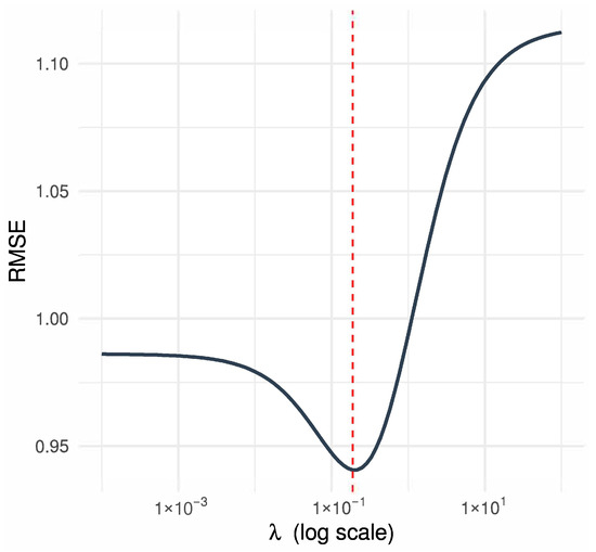
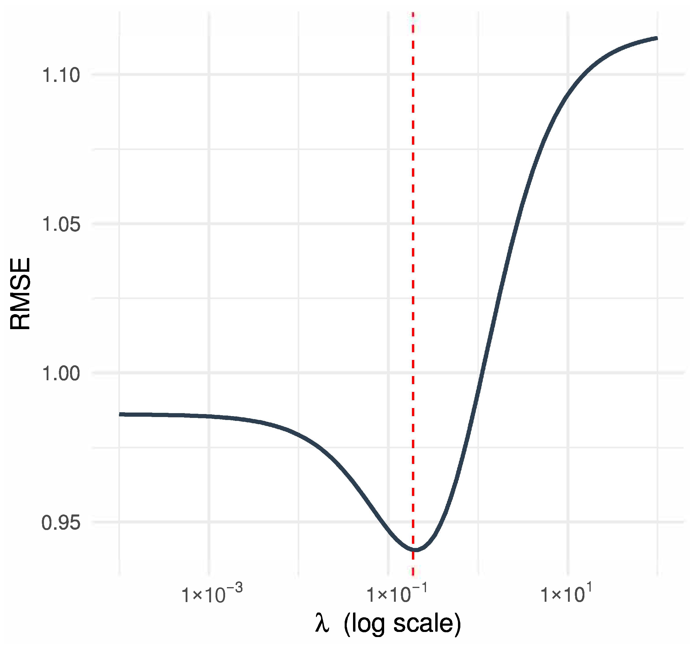
To apply our graph-based interpolation method, we need to specify the smoothing parameter $\lambda$. For this purpose, we used a 5-fold spatial block cross-validation procedure (Roberts et al., 2017 [17]). Specifically, we partitioned the observations into 5 spatial blocks based on their coordinates using K-means clustering (MacQueen, 1967 [18]). The optimal value of $\lambda$ was then selected from 100 logarithmically spaced points between ${10}^{-4}$ and ${10}^2$. As shown in Figure 2, the selected value, indicated by a red dashed line, is $\lambda =0.1874$.

Figure 2. Root mean squared error (RMSE) as a function of the smoothing parameter $\lambda$, evaluated via spatial block cross-validation. The optimal value of $\lambda$, indicated by a red dashed line, is $0.1874$.

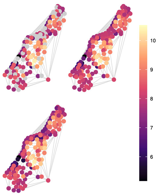
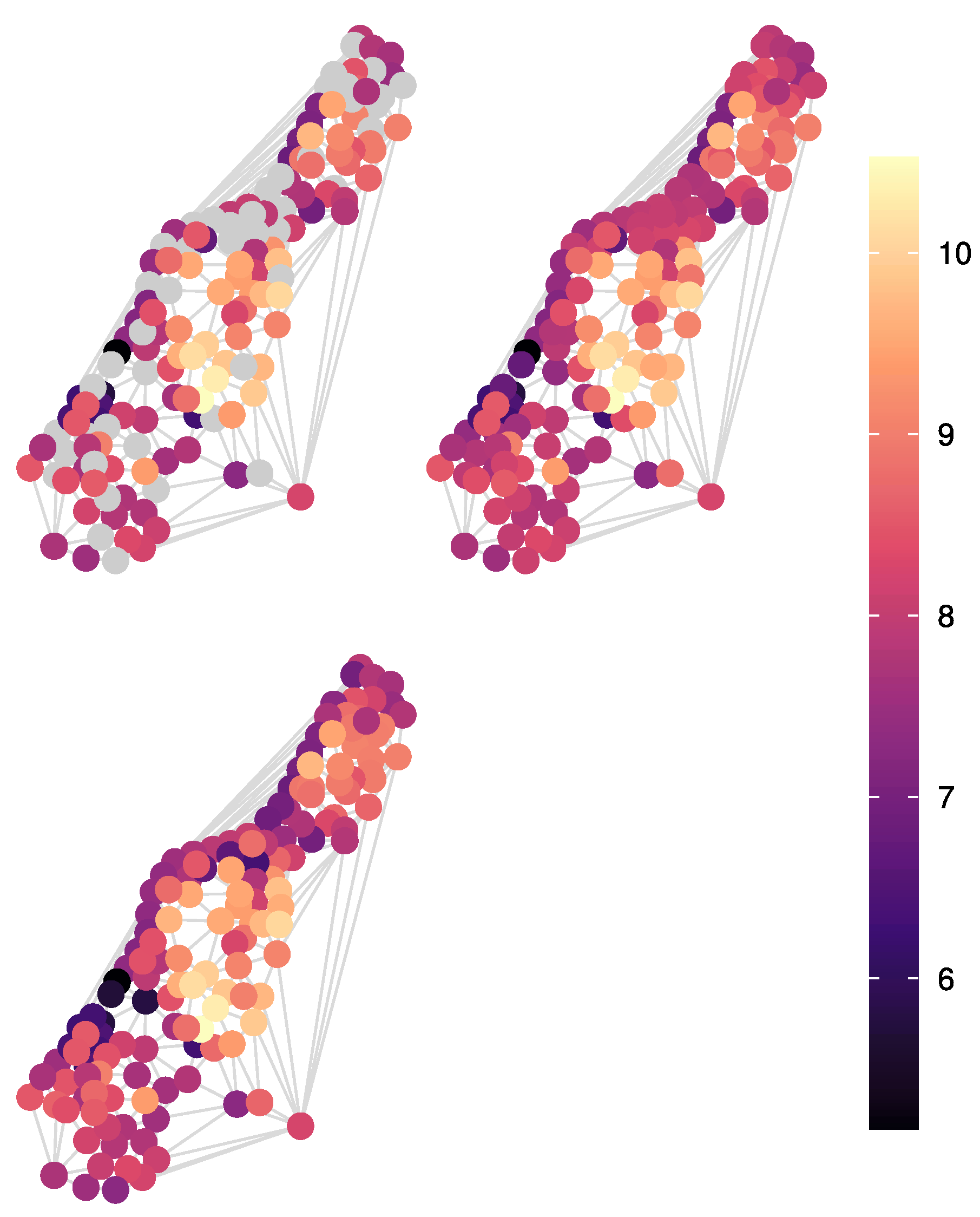
Figure 3 illustrates the performance of the proposed graph-based interpolation method. It shows the observed data with 30% of the values randomly removed (top left), the imputed data obtained using the proposed graph-based interpolation method (top right), and the original complete data (bottom left). The reconstructed values closely match the true elevations, indicating that the method provides highly accurate interpolations for spatially autocorrelated missing data.

Figure 3. Observed data with 30% of values randomly removed (top left), imputed data using the proposed graph-based interpolation method (top right), and the original complete data (bottom left).

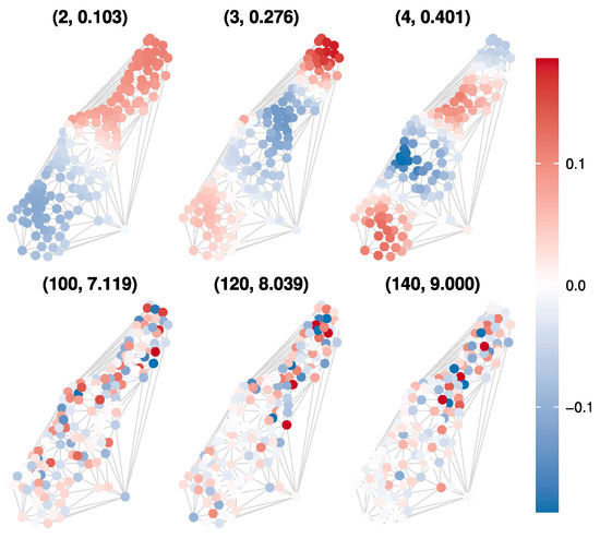
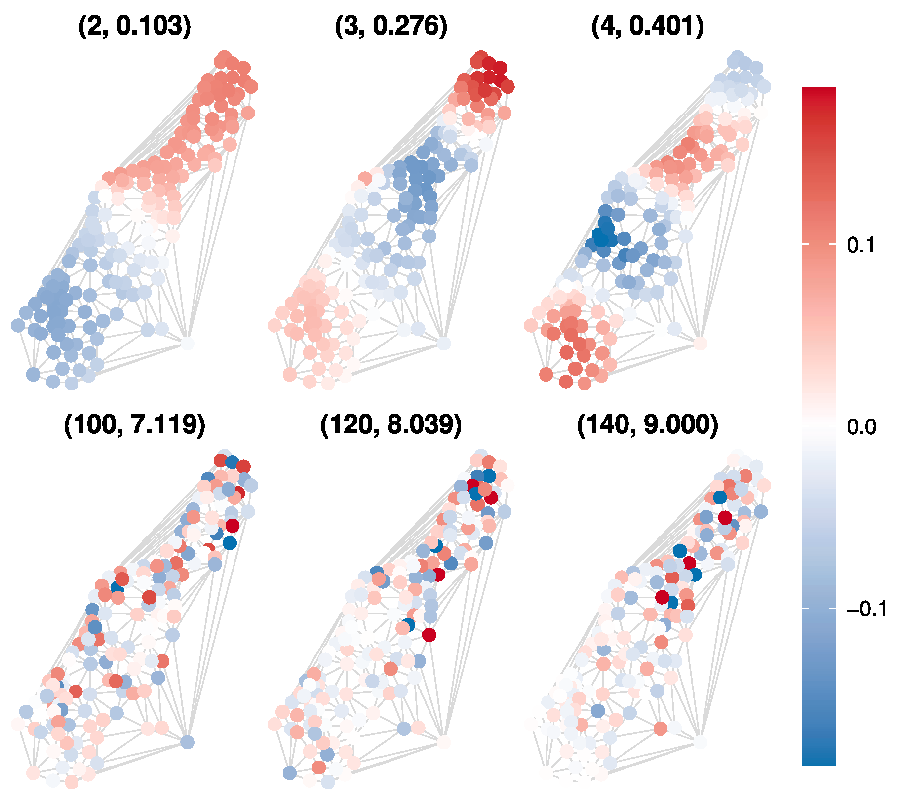
Finally, for reference, we present plots of several graph Laplacian eigenvectors. Figure 4 shows ${\mathit{p}}_i$ for $i=2,3,4,100,120,140$. In each panel, the first element of the ordered pair denotes the index i, and the second gives the value of ${\mathit{p}}_i^{\top }\mathit{L}{\mathit{p}}_i$. For instance, the top-left panel displays ${\mathit{p}}_2$ with ${\mathit{p}}_2^{\top }\mathit{L}{\mathit{p}}_2=0.103$. From this figure, it is clear that spatial autocorrelation is high when i is small, whereas it becomes low when i is large. In fact, as i increases, ${\mathit{p}}_i^{\top }\mathit{L}{\mathit{p}}_i$ strictly increases. This figure provides a visualization of the inequalities in (9) and (12).

Figure 4. Graph Laplacian eigenvectors ${\mathit{p}}_i$ for $i=2,3,4,100,120,140$. In each panel, the first element of the ordered pair denotes the index i, and the second gives the value of ${\mathit{p}}_i^{\top }\mathit{L}{\mathbf{p}}_i$.

6. Concluding Remarks

In this paper, we established a novel connection between spatial statistics and spectral graph theory. By exploiting the graph Laplacian eigenbasis that reflects the underlying graph structure, we showed that all missing values can be reconstructed, even from a single observation. This is made possible by the fact that the eigenvectors of the graph Laplacian can be ordered according to their spatial autocorrelation measured by Geary’s c. The main result of this study is presented in Theorem 1. We also provided an empirical illustration of our method, showing its practical effectiveness. These results highlight the usefulness of the graph Laplacian eigenbasis in spatial statistics and suggest promising directions for future developments.

Finally, although we derived the predictor ${\widehat{\mathit{y}}}_b$ for the missing-value vector ${\mathit{y}}_b$ in Theorem 1, the detailed properties of this predictor have not yet been investigated and are left for future work. Additionally, clarifying the advantages and disadvantages of the method proposed in this paper compared to other approaches, such as kriging, will be an important topic for future research.

References

- Yamada, H. Geary’s c and spectral graph theory: A complement. Mathematics 2023, 11, 4228. [Google Scholar] [CrossRef] [Scilit]
- Geary, R.C. The contiguity ratio and statistical mapping. Inc. Stat. 1954, 5, 115–145. [Google Scholar] [CrossRef] [Scilit]
- Cliff, A.D.; Ord, J.K. The problem of spatial autocorrelation. In Studies in Regional Science; Scott, A.J., Ed.; Pion: London, UK, 1969; pp. 25–55. [Google Scholar]
- Cliff, A.D.; Ord, J.K. Spatial autocorrelation: A review of existing and new measures with applications. Econ. Geogr. 1970, 46, 269–292. [Google Scholar] [CrossRef] [Scilit]
- Cliff, A.D.; Ord, J.K. Spatial Autocorrelation; Pion: London, UK, 1973. [Google Scholar]
- Cliff, A.D.; Ord, J.K. Spatial Processes: Models and Applications; Pion: London, UK, 1981. [Google Scholar]
- Von Neumann, J. Distribution of the ratio of the mean square successive difference to the variance. Ann. Math. Stat. 1941, 12, 367–395. [Google Scholar] [CrossRef] [Scilit]
- Hodrick, R.J.; Prescott, E.C. Postwar U.S. business cycles: An empirical investigation. J. Money Credit Bank. 1997, 29, 1–16. [Google Scholar] [CrossRef] [Scilit]
- Yamada, H. Trend extraction from economic time series with missing observations by generalized Hodrick–Prescott filters. Econom. Theory 2022, 38, 419–453. [Google Scholar] [CrossRef] [Scilit]
- Bapat, R.B. Graphs and Matrices, 2nd ed.; Springer: London, UK, 2014. [Google Scholar]
- Estrada, E.; Knight, P. A First Course in Network Theory; Oxford University Press: Oxford, UK, 2015. [Google Scholar]
- Gallier, J. Spectral theory of unsigned and signed graphs. Applications to graph clustering: A survey. arXiv 2016, arXiv:1601.04692. [Google Scholar] [CrossRef] [Scilit]
- Yamada, H. Geary’s c and spectral graph theory. Mathematics 2021, 9, 2465. [Google Scholar] [CrossRef] [Scilit]
- Beck, A. Introduction to Nonlinear Optimization Theory, Algorithms, and Applications with MATLAB; Society for Industrial and Applied Mathematics: Philadelphia, PA, USA, 2014. [Google Scholar]
- Yamada, H. Spatial smoothing using graph Laplacian penalized filter. Spat. Stat. 2024, 60, 100799. [Google Scholar] [CrossRef] [Scilit]
- Hoerl, A.E.; Kennard, R.W. Ridge regression: Biased estimation for nonorthogonal problems. Technometrics 1970, 12, 55–67. [Google Scholar] [CrossRef]
- Roberts, D.R.; Bahn, V.; Ciuti, S.; Boyce, M.S.; Elith, J.; Guillera-Arroita, G.; Hauenstein, S.; Lahoz-Monfort, J.J.; Schröder, B.; Thuiller, W.; et al. Cross-validation strategies for data with temporal, spatial, hierarchical, or phylogenetic structure. Ecography 2017, 40, 913–929. [Google Scholar] [CrossRef] [Scilit]
- MacQueen, J. Some methods for classification and analysis of multivariate observations. In Proceedings of the Fifth Berkeley Symposium on Mathematical Statistics and Probability, Volume 1: Statistics; University of California Press: Berkeley, CA, USA, 1967; pp. 281–297. [Google Scholar]
Disclaimer/Publisher’s Note: The statements, opinions and data contained in all publications are solely those of the individual author(s) and contributor(s) and not of MDPI and/or the editor(s). MDPI and/or the editor(s) disclaim responsibility for any injury to people or property resulting from any ideas, methods, instructions or products referred to in the content. |
© 2026 by the authors. Licensee MDPI, Basel, Switzerland. This article is an open access article distributed under the terms and conditions of the Creative Commons Attribution (CC BY) license.