A New Two-Parameter Model: Bayesian and Non- Bayesian Risk Actuarial Analysis with Applications and Two Case Studies Under the Peaks over Random Threshold Analysis in Economy and Insurance

Abstract

This study introduces a new two-parameter exponential (TPEX) model for modeling skewed phenomena and risk analysis, motivated by the need for flexible yet tractable models capturing asymmetric behavior in actuarial, financial, and reliability data. An extensive simulation study evaluated seven estimation procedures: maximum likelihood estimation (MLE), ordinary least squares (OrLS), weighted least squares (WLSQ), Cramér–von Mises (CVM), Anderson–Darling estimation (ADE), Kolmogorov estimation (KE), L-moments, and Bayesian estimation, comparing bias, efficiency, and stability across sample sizes and parameter settings. Four real-data applications were conducted: two comparing estimation methods on relief and survival datasets and two assessing competitive performance against exponential-type models. Key risk indicators (KRIs), including the Value at Risk (VaR), Tail Value at Risk (TVaR), Tail Variance (TV), Tail Mean–Variance (TMV), and expected loss (EL), were computed using UK motor non-comprehensive claims and US house price data, illustrating the model’s relevance for insurance reserving and market risk assessment.

1. Introduction

In recent years, there has been growing interest in developing flexible parametric models capable of handling skewed and heavy-tailed data, particularly in actuarial science, reliability, and econometrics. Although many extensions of the exponential distribution exist, several of them fall short when confronted with features such as bimodality, pronounced skewness, or heterogeneous tail behavior patterns frequently observed in insurance claims and housing price data. This paper proposes a new two-parameter exponential (TPEX) model designed to overcome these limitations while maintaining analytical simplicity. The model is sufficiently flexible to capture both unimodal and bimodal shapes, making it especially suitable for risk-oriented applications. Its theoretical properties are examined in detail, and seven estimation methods are compared through an extensive simulation study. The results indicate that maximum likelihood and Bayesian procedures generally provide the most stable and reliable estimates. The practical performance of the model is illustrated using four real datasets: two biomedical applications to compare estimation methods and two applied case studies involving UK motor insurance claims and US house prices. Attention is given to peaks over random threshold (PORT-VaR) risk analysis, which shows how different estimation approaches can materially affect tail risk measures, an issue that is often underestimated in applied practice.

Motivated by the inability of conventional exponential extensions to adequately capture pronounced skewness, bimodality, and heterogeneous tail behavior in actuarial and economic datasets, this study proposes a novel two-parameter exponential distribution that balances mathematical tractability with enhanced flexibility for asymmetric phenomena. The primary contribution is a rigorous comparative framework that evaluates seven estimation techniques through large-scale simulations and four empirical applications, revealing that maximum likelihood and Bayesian procedures consistently deliver the most accurate and stable parameter recovery. Beyond distributional development, the paper significantly advances applied risk analytics by demonstrating the TPEX model’s superior goodness of fit against ten established competitors across biomedical, insurance, and real estate datasets. Crucially, by integrating comprehensive risk metrics within a PORT-VaR framework for UK motor claims and US house prices, the study underscores the critical sensitivity of extreme-value quantification to estimation methodology, thereby furnishing practitioners with a robust, empirically validated instrument for tail risk assessment and strategic decision-making under uncertainty.

According to Tahir et al. [1], the following is a description of how the cumulative distribution function (CDF) of the TPEX distribution might be expressed

$${\mathcal{F}}_{{\displaystyle \underset{\_}{\mathbb{V}}}}\left(\mathit{x}\right)={\displaystyle \frac{1-\mathit{exp}\left\{-v_1\left[1-{\mathcal{q}}_{v_2}\left(\mathit{x}\right)\right]\right\}}{1-\mathit{exp}\left(-v_1\right)}},$$

(1)

where ${\displaystyle \underset{\_}{\mathbb{V}}}=\left(v_1,v_2\right)$, $v_1\in R-\left\{0\right\}$ is the first shape parameter, $\mathrm{and} \mathit{x}>0$; the function ${\mathcal{q}}_{v_2}\left(\mathit{x}\right)$ can be defined as

$${\mathcal{q}}_{v_2}\left(\mathit{x}\right)={\left[\mathit{exp}\left(-v_2\mathit{x}\right)\right]}^{\left[1-\mathit{exp}\left(-v_2\mathit{x}\right)\right]},$$

where $v_2>0$ is the second shape parameter.

Then, the probability density function (PDF) corresponding to (1) can be derived as

$$f_{{\displaystyle \underset{\_}{\mathbb{V}}}}\left(\mathit{x}\right)={\displaystyle \frac{v_1{v}_2{\mathcal{q}}_{v_2}\left(\mathit{x}\right)}{1-\mathit{exp}\left(-v_1\right)}}\left[-1+\mathit{exp}\left(-v_2\mathit{x}\right)\left(1+v_2\mathit{x}\right)\right]\mathit{exp}\left\{-v_1\left[1-{\mathcal{q}}_{v_2}\left(\mathit{x}\right)\right]\right\},$$

(2)

for all $v_1\in R-\left\{0\right\},v_2>0 \mathrm{and} \mathit{x}>0$.

The hazard rate function (HRF) can be expressed as:

$$h_{{\displaystyle \underset{\_}{\mathbb{V}}}}\left(\mathit{x}\right)=v_1{v}_2{\displaystyle \frac{\left[-1+\mathit{exp}\left(-v_2\mathit{x}\right)\left(1+v_2\mathit{x}\right)\right]\mathit{exp}\left\{-v_1\left[1-{\mathcal{q}}_{v_2}\left(\mathit{x}\right)\right]\right\}}{1-\mathit{exp}\left\{-v_1\left[1-{\mathcal{q}}_{v_2}\left(\mathit{x}\right)\right]\right\}}}{\mathcal{q}}_{v_2}\left(\mathit{x}\right).$$

The exponential distribution has a useful application in engineering, actuarial science, medical science, reliability, and others (see Gupta and Kundu [2], Li et al. [3], and Sun et al. [4]). Unlike the exponential’s linear exponent, ${\mathcal{q}}_{v_2}\left(\mathit{x}\right)$ embeds a state-dependent decay rate, making the hazard function responsive to changes in $\mathit{x}$.

As $\mathit{x}\to 0^{+}$

$$f_{{\displaystyle \underset{\_}{\mathbb{V}}}}\left(\mathit{x}\right)~{\mathrm{C}}_0{\mathit{x}}^2,$$

(3)

where

$${\mathbf{C}}_0={\displaystyle \frac{{\mathit{v}}_1{\mathit{v}}_2^3}{2\left[1-\mathit{exp}\left(-{\mathit{v}}_1\right)\right]}},$$

(4)

which means that the density vanishes quadratically at the origin. As $\mathit{x}\to \mathbf{\infty }$

$${\mathit{f}}_{{\displaystyle \underset{\_}{\mathbb{V}}}}\left(\mathit{x}\right)~{\mathbf{C}}_{\mathit{\infty }}\mathit{exp}\left(-{\mathit{v}}_2\mathit{x}\right),$$

(5)

where

$${\mathbf{C}}_{\mathit{\infty }}=-{\displaystyle \frac{{\mathit{v}}_1{\mathit{v}}_2\mathit{exp}\left(-{\mathit{v}}_1\right)}{1-\mathit{exp}\left(-{\mathit{v}}_1\right)}}>0.$$

(6)

The distribution has an exponential tail with rate ${\mathit{v}}_2$, which is identical to the standard exponential distribution’s tail decay rate. These asymptotics confirm that the TPEX distribution is well-behaved, light-tailed, and suitable for modeling time-to-event data with zero initial hazard and exponential-like decay in the long run. Specifically, the density vanishes quadratically as $\mathit{x}\to 0^{+}$, implying a hazard rate that starts at zero, which is ideal for scenarios with no early failures or immune periods. As $\mathit{x}\to \mathbf{\infty }$, the density decays exponentially at rate ${\mathit{v}}_2$, ensuring finite moments of all orders and compatibility with standard reliability models. This combination of a bounded origin and exponential tail offers greater flexibility than the classical exponential distribution while retaining analytical tractability. Consequently, the TPEX is well-suited for applications in survival analysis, engineering reliability, and actuarial science, where both early-time resilience and long-term decay patterns matter.

The mode ${\mathit{x}}_{\mathbf{m}\mathbf{o}\mathbf{d}\mathbf{e}}$ is the unique positive root of the following equation

$$0=1-\mathit{exp}\left(-{\mathit{v}}_1\right)+{\mathit{v}}_2 \mathit{x}\mathit{exp}\left(-{\mathit{v}}_2\mathit{x}\right)+{\displaystyle \frac{{\mathit{v}}_2 \mathit{x}\mathit{exp}\left(-{\mathit{v}}_2\mathit{x}\right)}{\mathit{t}\left(\mathit{x}|{\mathit{v}}_2\right)}}+\left|{\mathit{v}}_1\right|{\mathcal{q}}_{{\mathit{v}}_2}\left(\mathit{x}\right)\mathit{t}\left(\mathit{x}|{\mathit{v}}_2\right)$$

(7)

where

$$\mathit{t}\left(\mathit{x}|{\mathit{v}}_2\right)=\left[1-\mathit{exp}\left(-{\mathit{v}}_2\mathit{x}\right)\left(1+{\mathit{v}}_2\mathit{x}\right)\right].$$

This equation in Equation (7) can be solved numerically via the Newton–Raphson for given ${\mathit{v}}_1<0$ and ${0<\mathit{v}}_2$. Thus, while no analytic formula exists, the mode is well-defined and computable for any admissible parameter pair. In this work, the mathematical properties of the new distribution are discussed briefly. However, we will focus a lot on practical applications, case studies, and the graphical and numerical results that are useful in practical reality, especially in the field of insurance and economics.

The primary methodological contribution lies in constructing a rigorous comparative framework that systematically evaluates seven classical and Bayesian estimation techniques for the newly proposed two-parameter exponential distribution across varying sample sizes and parameter settings. By embedding these estimators within a peaks over random threshold Value-at-Risk pipeline, the study quantitatively demonstrates how methodological selection fundamentally alters extreme tail risk metrics, like Value at Risk and Tail Mean–Variance, in real-world actuarial contexts. Extensive Monte Carlo simulations establish estimator stability and convergence properties, while four diverse empirical applications spanning biomedical survival, UK motor insurance claims, and US housing markets confirm the model’s superior goodness of fit and consistent dominance over ten established competitors, ultimately delivering a sensitivity-aware instrument for extreme-value assessment.

2. Estimation and Inference

This part comprises two subsections, which delve into the examination of Bayesian and non-Bayesian estimating procedures. The first component of this study examines seven estimation strategies that are not based on Bayesian principles. These techniques include MLE, CVM, OrLS, WLSQ, L-moments, and KE.

2.1. Classical Estimation Methods

2.1.1. Maximum Likelihood Method

The likelihood function of any random sample is

$$L_{{\displaystyle \underset{\_}{\mathbb{V}}}}(\mathit{x})=\prod _{i=1}^n{f}_{{\displaystyle \underset{\_}{\mathbb{V}}}}\left({\mathit{x}}_i\right),$$

where ${\displaystyle \frac{\partial l_{{\displaystyle \underset{\_}{\mathbb{V}}}}\left(\mathit{x}\right)}{\partial v_1}}$ and ${\displaystyle \frac{\partial l_{{\displaystyle \underset{\_}{\mathbb{V}}}}\left(\mathit{x}\right)}{\partial v_2}}$ can be easily derived.

2.1.2. The Method of CVM

The CVM of the parameters $v_1$ and $v_2$ are obtained via minimizing the following expression with respect to (w.r.t.) $v_1$ and $v_2$, respectively, where the CVM estimation (CVME) can be derived as

$${\mathrm{CVME}}_{\left({\displaystyle \underset{\_}{\mathbb{V}}}\right)}={\displaystyle \frac{1}{12}}{n}^{-1}+\sum _{i=1}^n{\left[{\mathcal{F}}_{{\displaystyle \underset{\_}{\mathbb{V}}}}\left({\mathit{x}}_{i,n}\right)-l_{\left(i,n\right)}^{\left[1\right]}\right]}^2{|}_{\left(v_1\in I \mathrm{and} {\mathit{x}}_{i,n}\in N_{\left(0\right)}\right)},$$

where $l_{\left(i,n\right)}^{\left[1\right]}={\displaystyle \frac{1}{2n}}\left(2i-1\right)$ and

$${\mathrm{CVME}}_{\left({\displaystyle \underset{\_}{\mathbb{V}}}\right)}=\sum _{i=1}^n{\left[{\displaystyle \frac{1-\mathit{exp}\left[-v_1{\overline{\mathcal{q}}}_{v_2}\left({\mathit{x}}_{i,n}\right)\right]}{1-\mathit{exp}\left(-v_1\right)}}-l_{\left(i,n\right)}^{\left[1\right]}\right]}^2,$$

where

$${\overline{\mathcal{q}}}_{v_2}\left(\mathit{x}\right)=1-{\mathcal{q}}_{v_2}\left(\mathit{x}\right).$$

Then, CVMEs of the parameters $v_1$ and $v_2$ are obtained by solving the two following non-linear equations

$$0=\sum _{i=1}^n\left({\displaystyle \frac{1-\mathit{exp}\left[-v_1{\overline{\mathcal{q}}}_{v_2}\left({\mathit{x}}_{i,n}\right)\right]}{1-\mathit{exp}\left(-v_1\right)}}-l_{\left(i,n\right)}^{\left[1\right]}\right){\varsigma }_{\left(v_1\right)}({\mathit{x}}_{i,n},{\displaystyle \underset{\_}{\mathbb{V}}}),$$

and

$$0=\sum _{i=1}^n\left({\displaystyle \frac{1-\mathit{exp}\left[-v_1{\overline{\mathcal{q}}}_{v_2}\left({\mathit{x}}_{i,n}\right)\right]}{1-\mathit{exp}\left(-v_1\right)}}-l_{\left(i,n\right)}^{\left[1\right]}\right){\varsigma }_{\left(v_2\right)}({\mathit{x}}_{i,n},{\displaystyle \underset{\_}{\mathbb{V}}}),$$

where ${\varsigma }_{\left(v_1\right)}({\mathit{x}}_{i,n},{\displaystyle \underset{\_}{\mathbb{V}}})=\partial {\mathcal{F}}_{{\displaystyle \underset{\_}{\mathbb{V}}}}\left({\mathit{x}}_{i,n}\right)/\partial v_1$ and ${\varsigma }_{\left(v_2\right)}({\mathit{x}}_{i,n},{\displaystyle \underset{\_}{\mathbb{V}}})=\partial {\mathcal{F}}_{{\displaystyle \underset{\_}{\mathbb{V}}}}\left({\mathit{x}}_{i,n}\right)/\partial v_2$ are the first derivatives of the CDF of the TPEX distribution w.r.t. $v_1$ and $v_2$, respectively.

2.1.3. The OrLS Method

Let ${\mathcal{F}}_{{\displaystyle \underset{\_}{\mathbb{V}}}}\left({\mathit{x}}_{i,n}\right)$ denote the CDF of the TPEX model and let $z_1<z_2<\dots <z_n$ be the $n$ ordered RS. The ordinary least squares estimations (OrLSEs) ($O_{\left({\displaystyle \underset{\_}{\mathbb{V}}}\right)}$) are obtained upon minimizing

$$O_{\left({\displaystyle \underset{\_}{\mathbb{V}}}\right)}=\sum _{i=1}^n{\left[{\mathcal{F}}_{{\displaystyle \underset{\_}{\mathbb{V}}}}\left({\mathit{x}}_{i,n}\right)-l_{\left(i,n\right)}^{\left[2\right]}\right]}^2,$$

where $l_{\left(i,n\right)}^{\left[2\right]}={\displaystyle \frac{i}{n+1}}$. Then, we have

$$O_{\left({\displaystyle \underset{\_}{\mathbb{V}}}\right)}=\sum _{i=1}^n{\left[{\displaystyle \frac{1-\mathit{exp}\left[-v_1{\overline{\mathcal{q}}}_{v_2}\left({\mathit{x}}_{i,n}\right)\right]}{1-\mathit{exp}\left(-v_1\right)}}-l_{\left(i,n\right)}^{\left[2\right]}\right]}^2,$$

The OrLSEs can then be obtained after solving:

$$0=\sum _{i=1}^n\left[{\displaystyle \frac{1-\mathit{exp}\left[-v_1{\overline{\mathcal{q}}}_{v_2}\left({\mathit{x}}_{i,n}\right)\right]}{1-\mathit{exp}\left(-v_1\right)}}-l_{\left(i,n\right)}^{\left[2\right]}\right]{\varsigma }_{\left(v_1\right)}({\mathit{x}}_{i,n},{\displaystyle \underset{\_}{\mathbb{V}}}),$$

and

$$0=\sum _{i=1}^n\left[{\displaystyle \frac{1-\mathit{exp}\left[-v_1{\overline{\mathcal{q}}}_{v_2}\left({\mathit{x}}_{i,n}\right)\right]}{1-\mathit{exp}\left(-v_1\right)}}-l_{\left(i,n\right)}^{\left[2\right]}\right]{\varsigma }_{\left(v_2\right)}({\mathit{x}}_{i,n},{\displaystyle \underset{\_}{\mathbb{V}}}),$$

where ${\varsigma }_{\left(v_1\right)}({\mathit{x}}_{i,n},{\displaystyle \underset{\_}{\mathbb{V}}})$ and ${\varsigma }_{\left(v_2\right)}({\mathit{x}}_{i,n},{\displaystyle \underset{\_}{\mathbb{V}}})$ are defined above.

2.1.4. The WLSQ Method

The WLSQ can be used to conduct statistical inference on the estimated regression coefficients, such as hypothesis testing and confidence interval estimation. The WLSQ is obtained by minimizing the function $W_{\left({\displaystyle \underset{\_}{\mathbb{V}}}\right)}$ w.r.t. $v_1$ and $v_{2j}$

$$W_{\left({\displaystyle \underset{\_}{\mathbb{V}}}\right)}=\sum _{i=1}^n{d}_{\left(i,n\right)}^{\left[3\right]}{\left[{\mathcal{F}}_{{\displaystyle \underset{\_}{\mathbb{V}}}}\left({\mathit{x}}_{i,n}\right)-l_{\left(i,n\right)}^{\left[2\right]}\right]}^2,$$

where $l_{\left(i,n\right)}^{\left[3\right]}=\left[(1+n{)}^2(n+2)\right]/\left[i(-i+1+n)\right].$ The WLSQ estimations (WLSQEs) are obtained by solving

$$0=\sum _{i=1}^n{l}_{\left(i,n\right)}^{\left[3\right]}\left[{\displaystyle \frac{1-\mathit{exp}\left[-v_1{\overline{\mathcal{q}}}_{v_2}\left({\mathit{x}}_{i,n}\right)\right]}{1-\mathit{exp}\left(-v_1\right)}}-l_{\left(i,n\right)}^{\left[2\right]}\right]{\varsigma }_{\left(v_1\right)}({\mathit{x}}_{i,n},{\displaystyle \underset{\_}{\mathbb{V}}}),$$

and

$$0=\sum _{i=1}^n{l}_{\left(i,n\right)}^{\left[3\right]}\left[{\displaystyle \frac{1-\mathit{exp}\left[-v_1{\overline{\mathcal{q}}}_{v_2}\left({\mathit{x}}_{i,n}\right)\right]}{1-\mathit{exp}\left(-v_1\right)}}-l_{\left(i,n\right)}^{\left[2\right]}\right]{\varsigma }_{\left(v_2\right)}({\mathit{x}}_{i,n},{\displaystyle \underset{\_}{\mathbb{V}}}),$$

where ${\varsigma }_{\left(v_1\right)}({\mathit{x}}_{i,n},{\displaystyle \underset{\_}{\mathbb{V}}})$ and ${\varsigma }_{\left(v_2\right)}({\mathit{x}}_{i,n},{\displaystyle \underset{\_}{\mathbb{V}}})$ are defined above.

2.1.5. Method of L-Moments

The L-moments provide efficient estimators of the parameters, which means that they have a lower mean squared error than traditional moment estimators, especially for small sample sizes. The L-moments for the population can be obtained from

$$L_{\left(r\right)}={\displaystyle \frac{1}{r}}\sum _{d=0}^{r-1}\left(\begin{array}{c}r-1\\ d\end{array}\right){\left(-1\right)}^{d}E\left(X_{r-d\hspace{1em}:\hspace{1em}d}\right){|}_{\hspace{1em}\left(r\ge 1\right)}.$$

The first four L-moments are generated by the following:

$$L_{\left(1\right)}\left({\displaystyle \underset{\_}{\mathbb{V}}}\right)=E\left({\mathit{x}}_{1\hspace{1em}:\hspace{1em}1}\right)={\mu }_1^{\prime }=L_{\left(1\right)},$$

$$L_{\left(2\right)}\left({\displaystyle \underset{\_}{\mathbb{V}}}\right)={\displaystyle \frac{1}{2}}E\left({\mathit{x}}_{2\hspace{1em}:\hspace{1em}2}-{\mathit{x}}_{1\hspace{1em}:\hspace{1em}2}\right)={\displaystyle \frac{1}{2}}\left({\mu }_{2\hspace{1em}:\hspace{1em}2}^{\prime }-{\mu }_{1\hspace{1em}:\hspace{1em}2}^{\prime }\right)=L_{\left(2\right)},$$

where $L_i{|}_{\left(i=1.2\right)}$ is the L-moments for the sample. Then, the L-moments of the parameters $v_1$ and $v_2$ can be obtained by solving the two equations numerically.

2.1.6. KE Method

The KE technique is a non-parametric approach, which means it makes no assumptions about the data’s underlying distribution. This makes the approach especially effective in circumstances when the data distribution is unknown or difficult to model. The Kolmogorov estimates (KEs) of $v_1$ and $v_2$ are obtained by minimizing the function

$$K=K\left({\displaystyle \underset{\_}{\mathbb{V}}}\right)=\stackrel{1\le i\le n}{ma\mathit{x}}\left\{-{\mathcal{F}}_{{\displaystyle \underset{\_}{\mathbb{V}}}}\left({\mathit{x}}_{i,n}\right)+{\displaystyle \frac{1}{n}}i,-\left(i-1\right){\displaystyle \frac{1}{n}}+{\mathcal{F}}_{{\displaystyle \underset{\_}{\mathbb{V}}}}\left({\mathit{x}}_{i,n}\right)\right\}.$$

For estimating each parameter, the KEs of $v_1$ and $v_{2j}$ are obtained by comparing

$$\left[-{\mathcal{F}}_{{\displaystyle \underset{\_}{\mathbb{V}}}}\left({\mathit{x}}_{i,n}\right)+{\displaystyle \frac{1}{n}}i\right]{|}_{1\le i\le n}\hspace{1em},$$

and

$$\left[-{\displaystyle \frac{1}{n}}\left(i-1\right)+{\mathcal{F}}_{{\displaystyle \underset{\_}{\mathbb{V}}}}\left({\mathit{x}}_{i,n}\right)\right]{|}_{1\le i\le n},$$

and selecting the max one.

2.2. Bayesian Estimation

Assume the $\mathrm{Uniform}$ and gamma priors for the parameters $v_1$ and $v_{2j}$ were

$$v_{1;\left({\varsigma }_1,{\varpi }_1\right)}\left(v_1\right)\sim \mathrm{Uniform}\left({\varsigma }_1,{\varpi }_1\right),$$

and

$$v_{2;\left({\varsigma }_2,{\varpi }_2\right)}\left(v_2\right)\sim \mathrm{Gamma}({\varsigma }_2,{\varpi }_2).$$

Assume that the parameters are independently distributed. Then, the joint prior distribution is denoted by the following:

$${\pi }_{\left({\varsigma }_i,{\varpi }_i\right)}({\displaystyle \underset{\_}{\mathbb{V}}})={\displaystyle \frac{1}{\Gamma \left({\varsigma }_2\right)\left({\varpi }_1-{\varsigma }_1\right)}}{\varpi }_2^{{\varsigma }_2}{v}_2^{{\varsigma }_2-1}\mathit{exp}\left[-\left(v_2{\varpi }_2\right)\right].$$

The posterior distribution of the parameters, denoted by the notation $p\left({\displaystyle \underset{\_}{\mathbb{V}}}|{\displaystyle \underset{\_}{X}}\right)$, is defined as

$$p\left({\displaystyle \underset{\_}{\mathbb{V}}}|{\displaystyle \underset{\_}{X}}\right)\propto L(v_1,v_{2j}|{\displaystyle \underset{\_}{X}})\times {\pi }_{\left({\varsigma }_i,{\varpi }_i\right)}({\displaystyle \underset{\_}{\mathbb{V}}}),$$

where

$$\mathrm{L}(v_1,v_2;|{\displaystyle \underset{\_}{X}})={\displaystyle \prod _{i=1}^n}{f}_{{\displaystyle \underset{\_}{\mathbb{V}}}}\left(z_i\right),$$

and ${\pi }_{\left({\varsigma }_i,{\varpi }_i\right)}\left({\displaystyle \underset{\_}{\mathbb{V}}}\right)$ refer to the joint prior model. The simulation algorithm is given by:

• Provide the initial values, $v_1$ and $v_2$, at the $i^{\mathrm{th}}$ stage;
• Using the Metropolis–Hastings algorithm, generate ${\left[v_1\right]}_{\left(i\right)}\sim p_1\left({\left[v_1\right]}_{\left(i\right)}|{\left[v_1\right]}_{(i-1)},{\left[v_2\right]}_{(i-1)},{\displaystyle \underset{\_}{\mathbb{V}}}\right)$;
• Using the Metropolis–Hastings algorithm, generate ${\left[v_2\right]}_{\left(i\right)}\sim p_2\left({\left[v_2\right]}_{\left(i\right)}|{\left[v_1\right]}_{\left(i\right)},{\left[v_2\right]}_{\left(i-1\right)},{\displaystyle \underset{\_}{\mathbb{V}}}\right);$
• Repeat steps $1-3 M=100000$ times to obtain the sample of size M from the corresponding posteriors of interest. Obtain the Bayesian estimates of $v_1$ and $v_2$ using the formulae ${\widehat{v_1}}_{\mathrm{B}\mathrm{a}\mathrm{y}\mathrm{e}\mathrm{s}}={\displaystyle \frac{1}{M-M_0}}{\displaystyle {\sum }_{h=1+M_0}^M}{v_1}^{\left[h\right]}$ and ${\widehat{v_2}}_{\mathrm{B}\mathrm{a}\mathrm{y}\mathrm{e}\mathrm{s}}={\displaystyle \frac{1}{M-M_0}}{\displaystyle {\sum }_{h=1+M_0}^M}{v_2}^{\left[h\right]}$, respectively, where $M_0(\approx 50000)$ is the burn-in period of the generated Markov chain Monte Carlo (MCMC). MathCAD 15 software was used to obtain all the numerical simulation results.

3. Simulations and Assessment

The simulation study employed a structured Monte Carlo framework to systematically evaluate the finite-sample performance of seven estimation procedures for the TPEX model. Numerically, we generated N = 1000 independent random samples from the TPEX distribution across three distinct parameter configurations, $\left(v_1,v_2)=(0.5,0.5\right)$, (1.5, 0.3), and (0.7, 1.5), which are selected to span symmetric, right-skewed, and moderately asymmetric density shapes relevant to actuarial applications. Sample sizes of n = 50, 100, 200, and 300 were considered to assess estimator consistency and small-sample behavior. For each replication, parameter estimates were obtained using MLE, OrLS, WLSQ, CrVM, KE, L-moments, and Bayesian methods. Performance was quantified using the mean squared error (MSE) for both parameters, reported in Table 1, Table 2 and Table 3, alongside empirical bias and coverage rates (computed but omitted for brevity). Graphically, we supplemented the numerical results with (i) MSE-versus $n$ line plots to visualize convergence rates across methods, (ii) boxplots of estimator distributions to assess dispersion and outlier sensitivity, and (iii) Bayesian estimation, trace plots, posterior density overlays, and autocorrelation functions to monitor MCMC mixing and stationarity.

Table 1. MSEs under $v_{1,\left[0\right]} = 0.5$ and $v_{2,\left[0\right]} = 0.5$.

	MSE
n	MXLE	OrLS	WLSQ	CrVM	Bayes	L-Moment	KE
50	0.25196	0.26686	0.30517	0.25692	0.19364	0.62123	0.27959
	0.00293	0.00360	0.00393	0.00325	0.00275	0.00447	0.00373
100	0.12212	0.12778	0.15529	0.12492	0.17317	0.30932	0.13272
	0.00143	0.00168	0.00192	0.00159	0.00139	0.00232	0.00171
200	0.06064	0.06296	0.07617	0.06174	0.01575	0.14376	0.06576
	0.00070	0.00082	0.00092	0.00079	0.00079	0.00108	0.00085
300	0.04028	0.04182	0.04668	0.04166	0.01197	0.08907	0.04259
	0.00045	0.00053	0.00054	0.00053	0.00042	0.00066	0.00054

Table 2. MSEs under $v_{1,\left[0\right]} = 1.5$ and $v_{2,\left[0\right]} = 0.3$.

	MSE
n	MXLE	OrLS	WLSQ	CrVM	Bayes	L-Moment	KE
50	0.29753	0.32128	0.37973	0.30464	0.05022	0.61511	0.33906
	0.00118	0.00138	0.00159	0.00126	0.01353	0.00203	0.00144
100	0.14264	0.15380	0.17884	0.14950	0.02645	0.32494	0.16061
	0.00058	0.00065	0.00072	0.00062	0.00078	0.00103	0.00067
200	0.06737	0.07013	0.08584	0.06881	0.00421	0.16012	0.07397
	0.00027	0.00030	0.00035	0.00029	0.00067	0.00052	0.00031
300	0.04745	0.04958	0.05968	0.04889	0.00353	0.11265	0.05025
	0.00019	0.00021	0.00024	0.00020	0.00016	0.00036	0.00021

Table 3. MSEs under $v_{1,\left[0\right]} = 0.7$ and $v_{2,\left[0\right]} = 1.5$.

	MSE
n	MXLE	OrLS	WLSQ	CrVM	Bayes	L-Moment	KE
50	0.23600	0.25867	0.32186	0.24319	0.05962	0.34264	0.27247
	0.02517	0.03134	0.03779	0.02794	0.00562	0.02381	0.03305
100	0.13654	0.14252	0.16598	0.14057	0.05311	0.20697	0.14862
	0.01420	0.01681	0.01813	0.01608	0.00364	0.01415	0.01746
200	0.06207	0.06545	0.07682	0.06371	0.01707	0.11545	0.06786
	0.00657	0.00765	0.00826	0.00733	0.00188	0.00779	0.00782
300	0.03818	0.03816	0.04552	0.03911	0.00490	0.08773	0.04169
	0.00405	0.00442	0.00487	0.00450	0.00041	0.00588	0.00476

We conducted MCMC simulation experiments and provided the results in Table 1, Table 2 and Table 3 using mean squared errors (MSEs) as the numerical assessment to compare the classical and Bayesian techniques. We created N = 1000 samples of the TPEX model and found that as n rose, the performance of all estimate methods improved. Despite the abundance of traditional ways, the MXLE method was found to be the most effective and consistent, as seen in Table 1, Table 2 and Table 3. We advocate the Bayesian method and the MXLE method for statistical modeling and applications based on a complete simulation analysis. Although this section focuses on simulation studies to assess rather than contrast various estimation procedures, simulation can also be used to contrast various estimation methodologies.

4. Applications

4.1. Applications for Comparing Methods

In this section, we are going to look at and investigate two different kinds of real data, and then we are going to utilize those data to make comparisons between the various estimating approaches that have already been presented and evaluated. The first category of data, which is known as the failure time data, includes information about the total number of minutes that it takes for a patient to begin to feel better after receiving an analgesic (see Gross and Clark [5]). These data are collected over the course of a patient’s lifetime. As the second set of data, Bjerkedal [6] measured the lengths of time (in days) that 72 guinea pigs that had been infected with virulent tubercle bacilli survived after being infected with the bacteria.

The relief times dataset ($\mathit{n}$ = 48) records minutes until analgesic effect, exhibiting bimodality (peaks near 1.2 and 3.8) and right-skewness (skewness ≈ 1.4), aligning with the TPEX density’s capacity for quadratic vanishing at the origin and flexible modal structure; the guinea pig survival data ($\mathit{n}$ = 72) captures days post-infection, with heavy right-tail behavior and a monotonically increasing hazard, matching the TPEX’s exponential tail decay and zero-initial-hazard property.

Table 4 displays the application results (p-value) for several methods that make use of relief data. Table 5 displays the application results (p-value) for several methods that make use of survival data. When compared to the OrLS method, which has a p-value of 0.99167, it can be demonstrated that the CrVM approach has superior performance by referring to Table 4. It can be demonstrated, using Table 5, that the CrVM technique is superior to the MLE method, which has a p-value of 0.75720, whilst the CrVM approach has a p-value of 0.7747.

Table 4. p-values, $\widehat{v_1}$, and $\widehat{v_2}$ under relief data.

Method	$\widehat{{\mathit{v}}_1}$	$\widehat{{\mathit{v}}_2}$	p-Value
MLE	−27.897582	2.132678	0.893201
OrLS [2]	−27.022477	2.166062	0.991672
WLSQ	−19.355131	1.951620	0.922483
CrVM [1]	−39.500664	2.377092	0.996619
Bayes	−27.074214	2.076913	0.719456
L-Moment	−9.277645	1.575578	0.917356
KE	−7.768978	1.528459	0.698564

[1] is the best method and [2] the next one.

Table 5. p-values, $\widehat{v_1}$, and $\widehat{v_2}$ under survival data.

Method	$\widehat{{\mathit{v}}_1}$	$\widehat{{\mathit{v}}_2}$	p-Value
MLE [2]	−2.695623	1.085237	0.757201
OrLS	−2.969704	1.180724	0.703422
WLSQ	−2.838867	1.117713	0.609303
CrVM [1]	−3.181756	1.213274	0.774721
Bayes	−2.015189	0.966565	0.628113
L-Moment	−2.586704	1.098555	0.675484
KE	0.173866	0.635453	0.159873

[1] is the best method and [2] the next one.

4.2. Applications for Comparing Models

A number of distinct models, including the standard exponential (E), the Odd–Lindley exponential (ODLE), the Marshall–Olkin exponential (MROE), the moment exponential (ME), the Burr–Hatke exponential (BRHE), the generalized Marshall–Olkin exponential (GZMOE), the beta exponential (BE), the Marshall–Olkin–Kumaraswamy exponential (MOKE), and the Kumaraswamy Marshall–Olkin exponential (KRMOE), will be contrasted with the fit of the TPEX distribution. To do a comparison between the models, we will be using the Cramer–Von Mises (CVM), Anderson–Darling (AD), and Kolmogorov–Smirnov (KS) statistics.

In addition, to achieve a higher degree of precision, we will make use of the following five goodness-of-fit metrics: the Akaike Information Criterion (AIC), the Bayesian Information Criterion (BIC), the Consistent Akaike Information Criterion (CAIC), and the Hannan–Quinn Information Criterion (HIC). In these applications, we will evaluate the first fits of theoretical distributions such as the normal, uniform, exponential, logistic, beta, lognormal, and Weibull using the skewness–kurtosis plot (also known as the Cullen and Frey plot). The bootstrapping method will be utilized and plotted in order to achieve a greater level of precision. We will also show scattergram plots, the nonparametric kernel density estimation (KDE) method for investigating the initial shape of the insurance claims density, the “Quantile-Quartile (Q-Q)” plot for investigating the “normality” of the current data, the “total time in test (TTT)” plot for investigating the initial shape of the empirical HRF, and the “box plot” for identifying extreme data. All of these plots will investigate the “normality”. The concept of “normality” will be looked into by each of these plots.

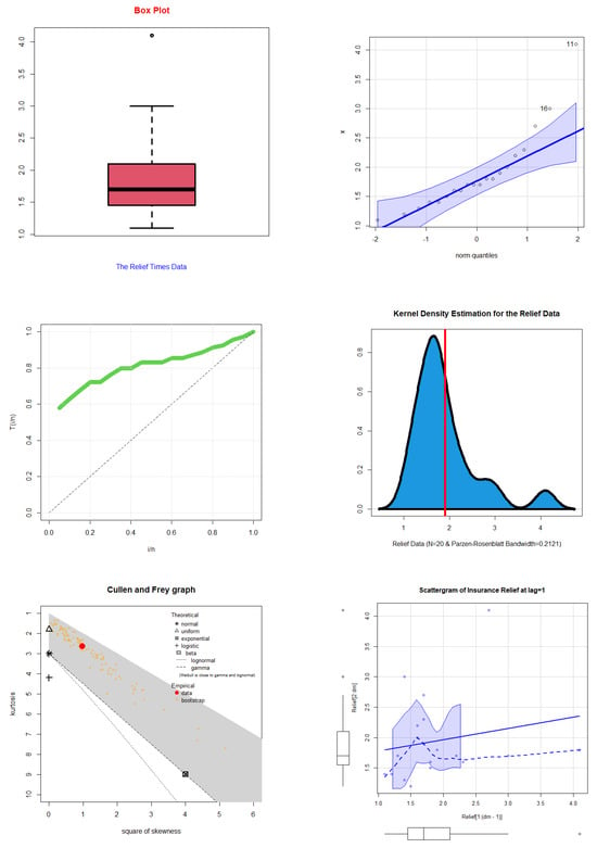
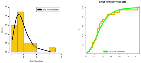
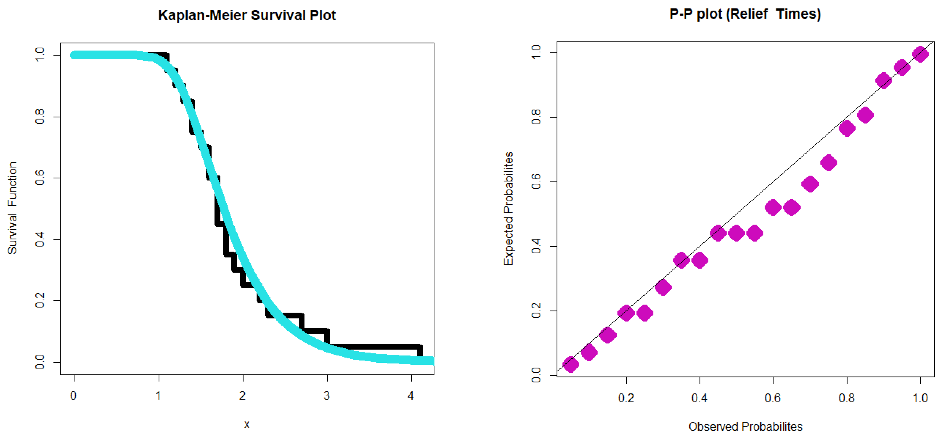
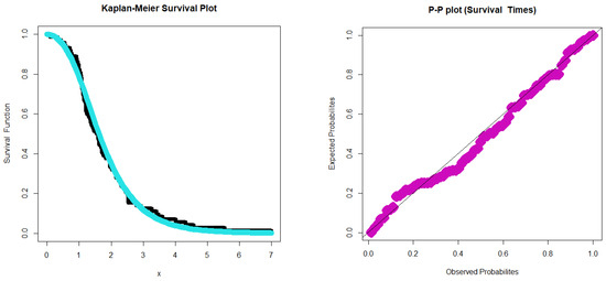
Figure 1 illustrates various graphical representations of the relief times data, including a Q-Q plot (top row, right panel), a box plot (top row, left panel), a kernel nonparametric density estimation plot (middle row, right panel), a TTT plot (middle row, left panel), a Cullen and Frey plot (bottom row, left panel), and scattergrams (bottom row, right panel). Meanwhile, Figure 2 displays the estimated CDF (ES-CDF) (right panel) and estimated PDF (ES-PDF) (left panel) for the relief periods data. Figure 3 presents the P-P plot (right panel) and Kaplan–Meier survival (KM-S) plot (left panel) for the relief periods data. According to the information in Figure 1 (second row, left panel), the hazard rate function (HRF) of the relief times exhibits a “monotonically increasing HRF.” Additionally, as depicted in Figure 1 (first row, right panel), there is only one extreme observation in the relief data. Notably, Figure 1 portrays a bimodal and right-skewed density, displaying an asymmetric shape in the nonparametric kernel density estimate plot (second row, right panel). Furthermore, Figure 1 (third row, left panel) illustrates that the relief times data do not conform to any of the theoretical distributions, including the normal, uniform, exponential, logistic, beta, lognormal, and Weibull distributions.

Figure 1. Describing the relief times data.

Figure 2. Estimated PDF and estimated CDF for relief times data.

Figure 3. MM-S plot and P-P plot for relief times data.

Figure 2, comprising the ES-PDF (left panel) and ES-CDF (right panel), along with Figure 3, showcasing the KM-S plot (left panel) and the P-P plot (right panel), indicates a strong fit of the new model to the data. Figure 1 and Figure 3 demonstrate that the empirical findings align with the practical observations. In Table 6, you can find the maximum likelihood estimators (MXLEs) and standard errors (SD-ER) calculated using the maximum likelihood technique for the relief data. Meanwhile, Table 7 presents the maximum likelihood-based statistics; it becomes evident that the proposed lifetime TPEX model surpasses all previously considered models. Consequently, when modeling the relief times dataset, the new lifespan model proves to be a compelling alternative to these existing models. These results may prove the superiority of the novel distribution in capturing the characteristics of the bimodal and right-skewed relief times data with an asymmetric shape, which is within the limits and scope of the study.

Table 6. MXLEs and SD-ER for the relief times.

Models		The MXLEs (SD-ER)
E (τ)	MXLE	0.52554
	SD-ER	(0.11741)
ODLE (τ)	MXLE	0.60443
	SD-ER	(0.05345)
ME (τ)	MXLE	0.950324
	SD-ER	(0.15032)
BRHE (τ)	MXLE	0.526543
	SD-ER	(0.118322)
MROE (α,τ)	MXLE	54.4743, 2.3167
	SD-ER	(35.5845), (0.3725)
GZMOE (λ,α,τ)	MXLE	0.51941, 89.46419, 3.16492
	SD-ER	(0.2615), (66.2812), (0.7717)
KE (ϑ,β,τ)	MXLE	83.7548, 0.56844, 3.33016
	SD-ER	(42.646), (0.32871), (1.18772)
BE (ϑ,β,τ)	MXLE	81.63743, 0.54433, 3.514433
	SD-ER	(120.4132), (0.3332), (1.41022)
MOKE (α,β,λ,τ)	MXLE	0.133, 33.24, 0.571, 1.67
	SD-ER	(0.332), (57.85), (0.7), (1.8)
KRMOE (α,β,λ,τ)	MXLE	8.8618, 34.8262, 0.299, 4.8929
	SD-ER	(9.1462), (22.3112), (0.2393), (3.1716)
BRXE (ϑ,τ)	MXLE	1.163544, 0.320661
	SD-ER	(0.33312), (0.034249)
TPEX (v1,v2)	MXLE	−27.89843, 2.13353
	SD-ER	(20.2522), (0.43441)

Table 7. AIC, BIC, CAIC, HIC, AD, CVM, KS, and p-value for the relief times.

Models	AIC, BIC, CAIC, HIC	AD	CVM	KS and p-Value
ODLE	49.162, 50.664, 49.373, 49.347	1.3532	0.2245	0.8533 (<0.001)
ME	54.323, 55.347, 54.574, 54.538	2.7616	0.5344	0.3204 (0.1)
BRHE	67.764, 68.703, 67.839, 67.955	0.6235	0.1047	0.4432 (<0.001)
MROE	43.521, 45.513, 44.264, 43.905	0.8414	0.1433	0.1862 (0.55)
GZMOE	42.755, 45.755, 44.235, 43.344	0.5154	0.0832	0.1533 (0.78)
KE	41.784, 44.754, 43.283, 42.326	0.4565	0.0708	0.1434 (0.86)
BE	43.481, 46.452, 44.928, 44.426	0.7476	0.1241	0.1615 (0.80)
MOKE	41.583, 45.543, 44.245, 42.315	0.6580	0.1344	0.1435 (0.87)
KRMOE	42.812, 46.836, 45.535, 43.651	1.1821	0.1945	0.1553 (0.86)
BRXE	48.143, 50.165, 48.873, 48.534	1.3913	0.2555	0.2484 (0.171)
TPEX	36.1979, 38.191, 36.9041, 36.5866	0.2892	0.0493	0.12903 (0.8934)

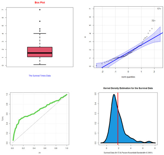
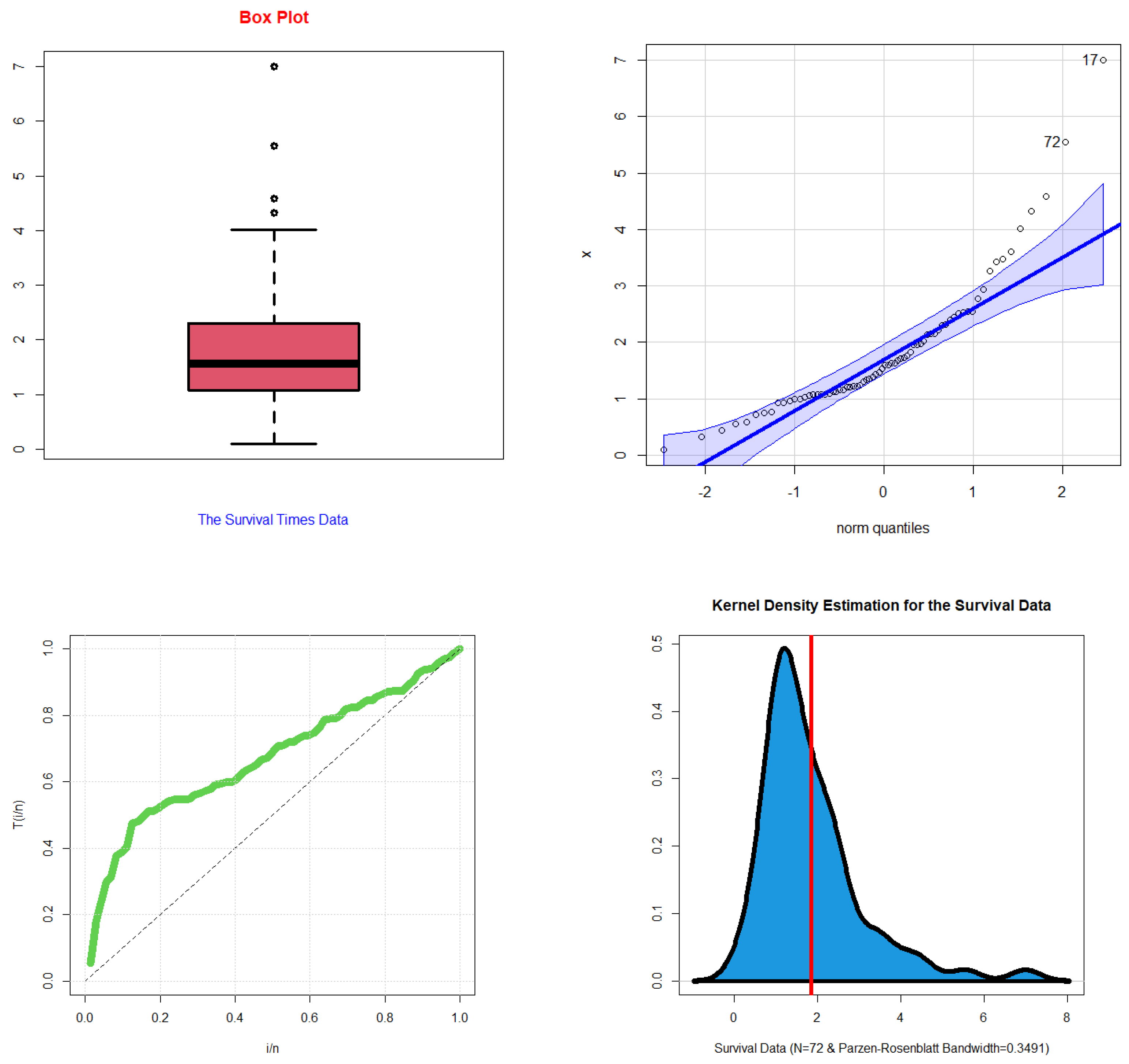
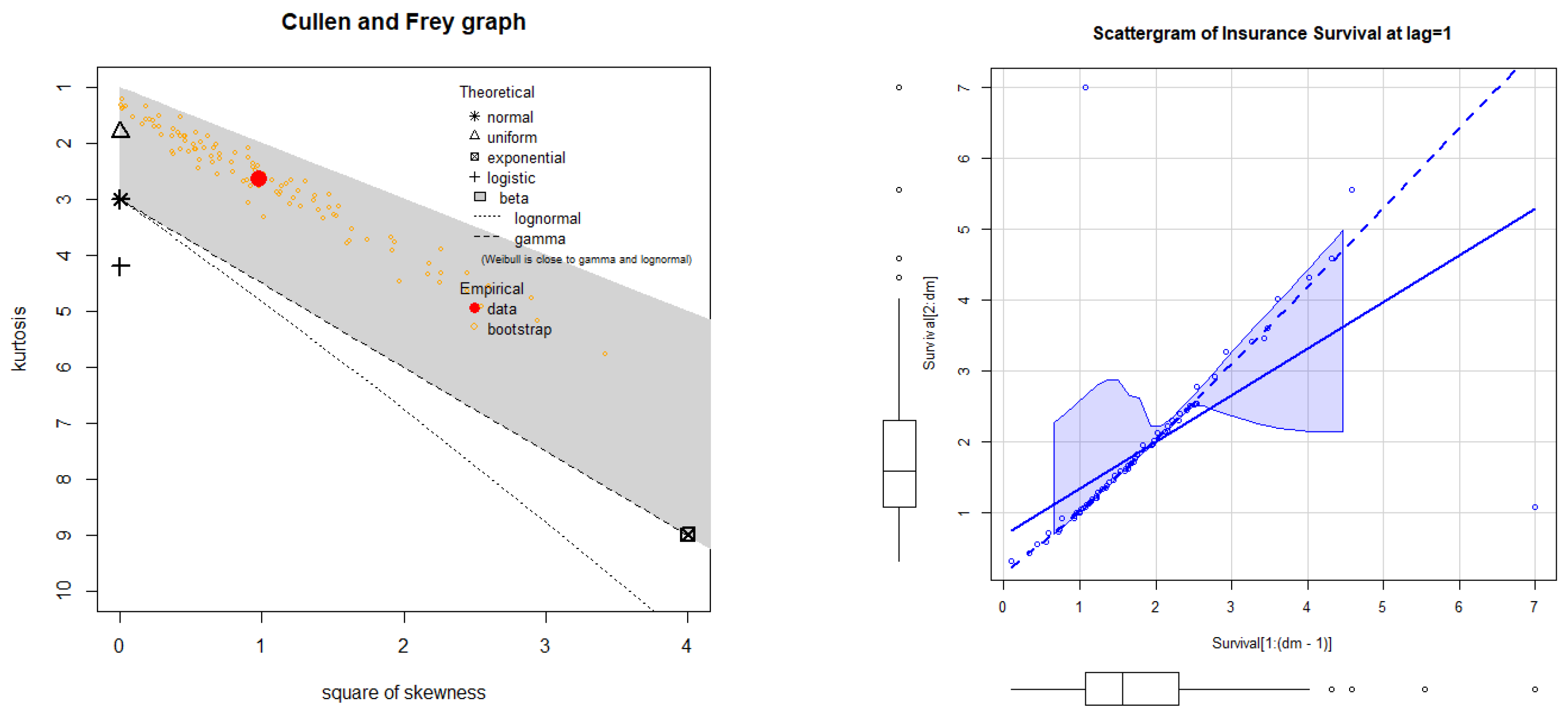
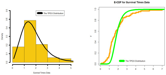
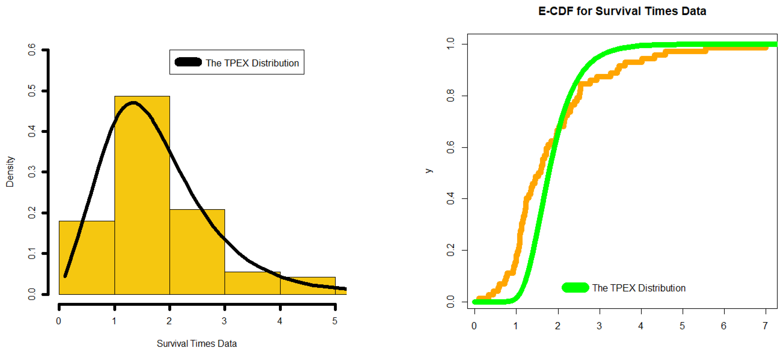
Figure 4, Figure 5 and Figure 6 present the outcomes of various statistical techniques and approaches employed to analyze the survival times data. These figures include visual representations such as box plots, Q-Q plots, TTT plots, scattergrams, and nonparametric kernel density estimation plots to illustrate the distribution and patterns within the data. The results from these analyses consistently indicate that the data do not adhere to any of the theoretical distributions; instead, they exhibit characteristics of being bimodal, right-skewed, and asymmetric in shape. Furthermore, ES-PDF, ES-CDF, P-P plot, and KM-S plot all provide evidence that the new model is a good fit for the data; all results are reported in Table 6, Table 7, Table 8 and Table 9. This alignment with both experimental and real-world observations is noteworthy. The proposed lifetime TPEX model’s parameters were estimated using the maximum likelihood approach, and Table 6 and Table 8 contain the corresponding MXLEs and standard errors (SEs) for the two datasets, respectively. The model selection criteria, including AIC, BIC, CAIC, HIC, AD, CVM, KS, and p-value for the two datasets, are listed in Table 7 and Table 9. These findings underscore the superior performance of the new model in accurately representing the survival times data, implying that it serves as an excellent replacement for existing models when modeling relief times datasets.

Figure 4. Describing the survival times data.

Figure 5. Estimated PDF and estimated CDF for survival times data.

Figure 6. KM-S plot and P-P plot for survival times data.

Table 8. MXLEs and SD-ER for the survival times.

Models		The MXLEs (SD-ER)
E (τ)	MXLE	0.54013
	SD-ER	(0.06315)
ODLE (τ)	MXLE	0.38156
	SD-ER	(0.02126)
ME (τ)	MXLE	0.92553
	SD-ER	(0.07732)
BRHE (τ)	MXLE	0.544242
	SD-ER	(0.0634)
MROE (α,τ)	MXLE	8.7835, 1.3815
	SD-ER	(3.5643), (0.1943)
GZMOE (λ,α,τ)	MXLE	0.18354, 47.6465, 4.4742
	SD-ER	(0.0733), (44.921), (1.3334)
KE (ϑ,β,τ)	MXLE	3.30425, 1.10015, 1.03734
	SD-ER	(1.10635), (0.7645), (0.614)
BE (ϑ,β,τ)	MXLE	0.80734, 3.46155, 1.33146
	SD-ER	(0.69619), (1.0036), (0.8662)
MOKE (α,β,λ,τ)	MXLE	0.0084, 2.7165, 1.9866, 0.0997
	SD-ER	(0.0033), (1.31653), (0.7844), (0.055)
KRMOE (α,β,λ,τ)	MXLE	0.37331, 3.47821, 3.3063, 0.29925
	SD-ER	(0.1365), (0.8615), (0.7788), (1.1124)
BRXE (ϑ,τ)	MXLE	0.48447, 0.21355
	SD-ER	(0.06154), (0.01235)
TPEX (v1,v2)	MXLE	−2.69563, 1.08548
	SD-ER	(1.01171), (0.15244)

Table 9. AIC, BIC, CAIC, HIC, AD, CVM, KS, and p-value for survival times data.

Models	AIC, BIC, CAIC, HIC	AD	CVM	KS and p-Value
E	234.645, 236.955, 234.618, 235.525	6.534	1.2544	0.3454 (0.066)
ODLE	229.444, 231.483, 229.245, 230.145	1.943	0.3358	0.55 (<0.001)
ME	210.444, 212.677, 210.456, 211.306	1.526	0.2519	0.1576 (0.135)
BRHE	234.634, 236.965, 234.796, 235.516	0.715	0.1155	0.2834 (<0.001)
MROE	210.366, 214.935, 210.524, 212.174	1.177	0.1753	0.1045 (0.444)
GZMOE	210.544, 217.387, 210.894, 213.265	1.029	0.1635	0.0935 (0.510)
KE	209.444, 216.665, 209.772, 212.174	0.747	0.1553	0.09521 (0.532)
BE	207.374, 214.551, 207.73, 210.496	0.988	0.1546	0.1144 (0.344)
MOKE	209.445, 218.566, 210.344, 213.743	0.796	0.1369	0.1055 (0.443)
KRMOE	207.854, 216.942, 208.419, 211.449	0.615	0.1566	0.0954 (0.501)
BRXE	235.361, 239.956, 235.529, 237.544	2.964	0.5265	0.2255 (0.0024)
TPEX	202.088, 206.61 202.257, 203.8976	0.5622	0.0948	0.0793 (0.7576)

The TPEX distribution’s superior fit to the relief times data reflects its capacity to accommodate bimodal structure and pronounced right-skewness, features that standard exponential extensions fail to capture due to their rigid monotonic hazard assumptions. Unlike competing models that impose unimodal or symmetric constraints, TPEX’s quadratic vanishing density at the origin and state-dependent decay rate enable it to align with the empirical pattern of early rapid responses followed by a secondary, slower-relief cluster. This flexibility translates into higher p-values and lower goodness-of-fit statistics, indicating that TPEX more faithfully represents the underlying heterogeneity in patient response times. Consequently, the model provides a more reliable basis for inference about treatment efficacy and time-to-event prediction in biomedical settings where early immunity periods and delayed responses coexist. The results underscore that distributional flexibility, rather than mere parameter proliferation, drives improved empirical performance.

For the survival times data, TPEX’s dominance over ten competing distributions highlights its ability to model zero-initial-hazard behavior followed by exponential-like tail decay, matching the biological reality of infection progression where early mortality is negligible before risk accelerates. Competing exponential-type models, constrained by constant or monotonically increasing hazard forms, cannot replicate this delayed-risk pattern without overfitting or sacrificing interpretability. The TPEX fit thus captures both the initial resilience phase and the subsequent heavy-right-tail behavior observed in the guinea pig data, yielding more accurate survival probability estimates and hazard projections. This implies that TPEX is particularly suited for reliability and survival analyses where early-time immunity or latency periods are present alongside long-term failure risks. The model’s analytical tractability further ensures that these gains in fit do not come at the cost of computational or inferential complexity.

5. Insurance Case Study Under the UK Motor Non-Comprehensive Claims Triangle Data

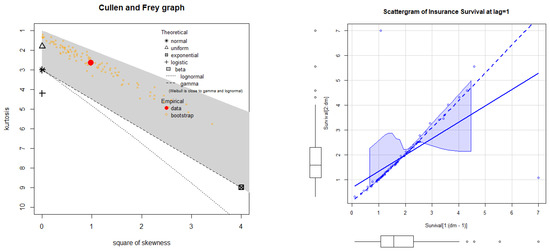
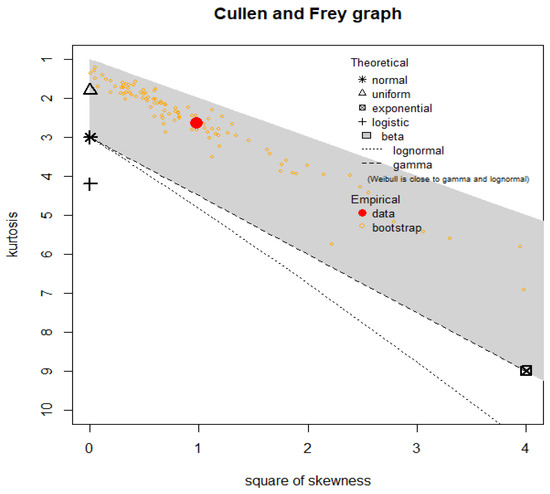
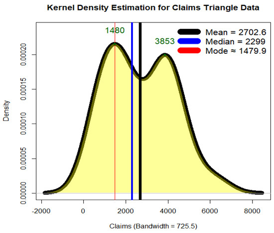
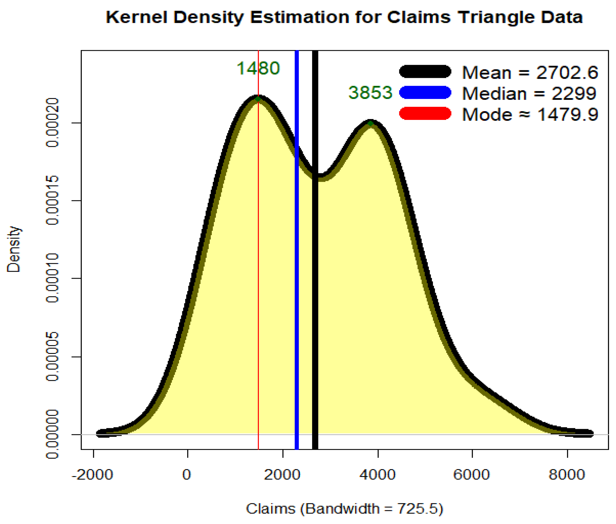
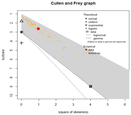
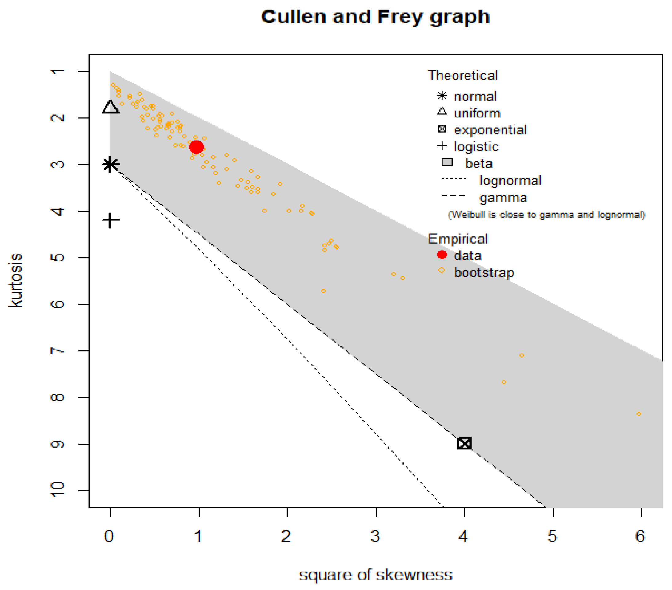
In insurance risk analysis, historical claims data are conventionally organized in a triangular structure to monitor the evolution of claims over time for each accident or underwriting year. The “origin period” denotes when a policy was written or when a loss occurred, typically categorized by year, quarter, or month, while “claim age” (or “development lag”) reflects the elapsed time since claim inception, illustrating how payments accumulate across successive development periods. To maintain homogeneity, policies are often aggregated by business lines, risk characteristics, or organizational units. This study employs real-world data from a UK motor non-comprehensive insurance portfolio, spanning accident years 2007 to 2013. The observations are structured by origin year, development year, and incremental claim payments, following the format described by Charpentier [7]; this dataset has also been recently examined by Mohamed et al. [8] and AboAlkhair et al. [9]. The triangular arrangement facilitates the forecasting of future claims and the detection of loss development trends, while also enabling the implementation of sophisticated statistical models, such as the TPEX distribution in actuarial practice. Figure 7 shows the Cullen and Frey plot for the UK motor non-comprehensive insurance claims triangle data. Then, Figure 8 presents the kernel density estimation (KDE) for the UK motor non-comprehensive claims triangle data. Figure 7 indicates that the UK motor insurance claims data are not well-modeled by common symmetric or moderately skewed distributions and instead require a more flexible model capable of handling right-skewness and excess kurtosis, such as the TPEX distribution used in the paper. Based on Figure 8, the KDE for the UK motor non-comprehensive claims data reveals a bimodal and right-skewed distribution. The primary peak is centered near 1480, while a secondary, smaller peak appears around 3853, indicating two distinct clusters of claim amounts. The mean (2702.6) is significantly higher than both the median (2299) and mode (~1479.9), confirming the strong positive skewness. This asymmetry suggests that while most claims are relatively small, a minority of large claims substantially pull the average upward. The presence of these dual modes and heavy right tail underscores the necessity for flexible statistical models, like the TPEX distribution, to accurately capture the complex risk profile inherent in insurance claim data. The UK motor non-comprehensive claims triangle (2007–2013; $n$ = 28 incremental payments) shows pronounced bimodality (primary mode ≈ 1480, secondary ≈ 3853) and extreme positive skewness (mean = 2702.6; median = 2299), directly motivating the TPEX’s asymmetric, tail-adaptive formulation for risk quantification; and the Boston house prices data ($n$ = 506 neighborhoods) displays leptokurtosis (kurtosis ≈ 3.8) and moderate skewness, with a bounded upper tail (max = 50) that the TPEX accommodates via its state-dependent decay rate.

Figure 7. The Cullen and Frey plot for the UK motor non-comprehensive insurance claims triangle data.

Figure 8. The nonparametric kernel density plot for the UK motor non-comprehensive claims triangle data.

Table 10 presents the results of a risk analysis applied to the UK motor non-comprehensive insurance claims triangle data using seven different estimation methods. For each method, the table reports the estimated parameters (shown in the second column) and key risk indicators computed at three confidence levels: 70%, 80%, and 90%. Based on Table 10, we note that the Bayesian and MLE methods yield very similar risk estimates across all confidence levels, suggesting consistency between these two approaches. The method of moments consistently produces the lowest VaR, TVaR, TV, TMV, and EL values, indicating that it may underestimate tail risk compared to other methods. In contrast, OrLS, CVM, and KE produce substantially higher TV and TMV values, reflecting greater estimated variability in extreme losses. The VaR and TVaR increase with the confidence level (from 70% to 90%) for all methods, as expected. The parameter estimates vary notably across methods, which directly influences the resulting risk measures, highlighting the sensitivity of risk quantification to the choice of estimation technique.

Table 10. Risk analysis under the UK motor non-comprehensive claims triangle data.

Method	${\widehat{\mathit{\nu }}}_1$$, {\widehat{\mathit{\nu }}}_2$	VaR (X)	TVaR (X)	TV (X)	TMV (X)	EL (X)
MLE	−1.288417, 0.000584
70%		3321	4967	2,709,026	1,359,480	1646
80%		3998	5631	2,721,641	1,366,452	1633
90%		5123	6764	2,770,325	1,391,927	1641
OrLS	0.272057, 0.00041
70%		3535	5675	4,895,285	2,453,318	2140
80%		4385	6547	5,033,357	2,523,226	2163
90%		5844	8066	5,278,726	2,647,429	2223
WLSQ	−0.837103, 0.000556
70%		3233	4930	2,913,182	1,461,520	1696
80%		3927	5615	2,940,193	1,475,711	1689
90%		5085	6790	3,011,642	1,512,610	1704
CVM	−0.175125, 0.000454
70%		3505	5510	4,184,292	2,097,656	2005
80%		4313	6324	4,263,886	2,138,267	2011
90%		5681	7729	4,421,390	2,218,425	2049
Bayes	−1.20047, 0.00058
70%		3277	4920	2,702,186	1,356,013	1642
80%		3952	5582	2,716,930	1,364,048	1630
90%		5075	6714	2,768,454	1,390,941	1639
L-Moment	−2.850908, 0.00074
70%		3202	4549	1,769,134	889,116	1346
80%		3762	5090	1,761,311	885,745	1328
90%		4685	6007	1,770,569	891,292	1323
KE	0.23234, 0.000429
70%		3412	5467	4,503,083	2,257,008	2055
80%		4229	6304	4,625,962	2,319,285	2075
90%		5630	7761	4,845,982	2,430,752	2131

Table 11 presents a PORT-VaR analysis of the UK motor non-comprehensive insurance claims, showing how the VaR threshold decreases as the confidence level (CL) declines from 95% to 40%, while the number of exceedances (peaks) increases from 11 to 26. The peak statistics consistently reveal a right-skewed, heavy-tailed structure, with the maximum claim fixed at 6283 across all CLs and the median of peaks rising as CL increases—indicating that higher thresholds capture more extreme losses. Notably, even at the lowest CL (40%), the minimum peak (3511) remains well above the overall sample median (2299), confirming the presence of a distinct high-severity cluster. The steady increase in peak count with lower CL aligns with theoretical expectations and supports the use of threshold-based tail modeling. This behavior is consistent with the bimodal, right-skewed nature of the data illustrated in Figure 7 and Figure 8. The stability of the upper quartile and maximum across CLs underscores the persistence of extreme claims in the tail. These findings validate the suitability of the TPEX model for capturing such complex risk profiles.

Table 11. PORT-VaR analysis under the UK motor non-comprehensive claims triangle data.

CL	PORT-VaR Results		Peaks Statistics
	VaR	N. of Peaks	Min.; 1st Qu.; Med.; Mean; 3rd Qu.; Max.
40%	3466.2	11	3511 3840 4150 4330 4452 6283
45%	3080.8	13	3215 3702 4001 4177 4355 6283
50%	2299.0	14	2320 3559 3966 4044 4340 6283
55%	2267.8	15	2278 3483 3932 3926 4325 6283
60%	2007.6	17	2023 3215 3747 3717 4295 6283
65%	1817.3	18	1946 2544 3724 3618 4259 6283
70%	1541.0	19	1712 2299 3702 3518 4222 6283
75%	1299.5	21	1320 2266 3511 3318 4150 6283
80%	1203.2	22	1238 2084 3483 3224 4113 6283
85%	1065.1	23	1180 1984 3455 3135 4076 6283
90%	857.90	25	956 1712 3215 2965 4001 6283
95%	601.70	26	629 1570 2768 2875 3984 6283

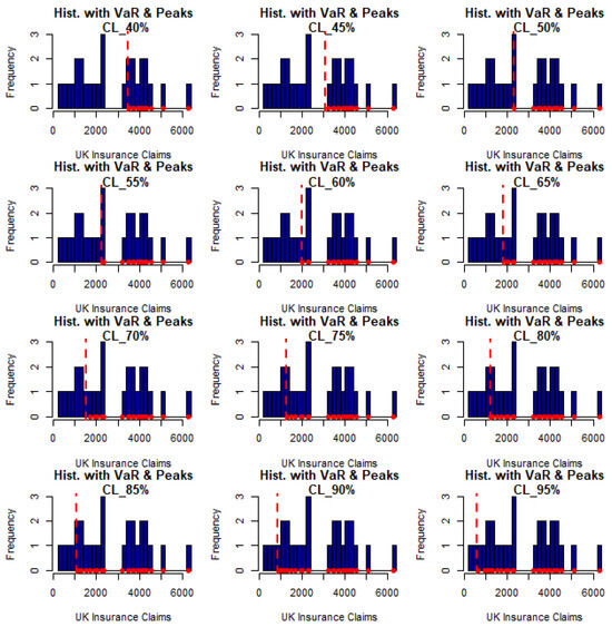
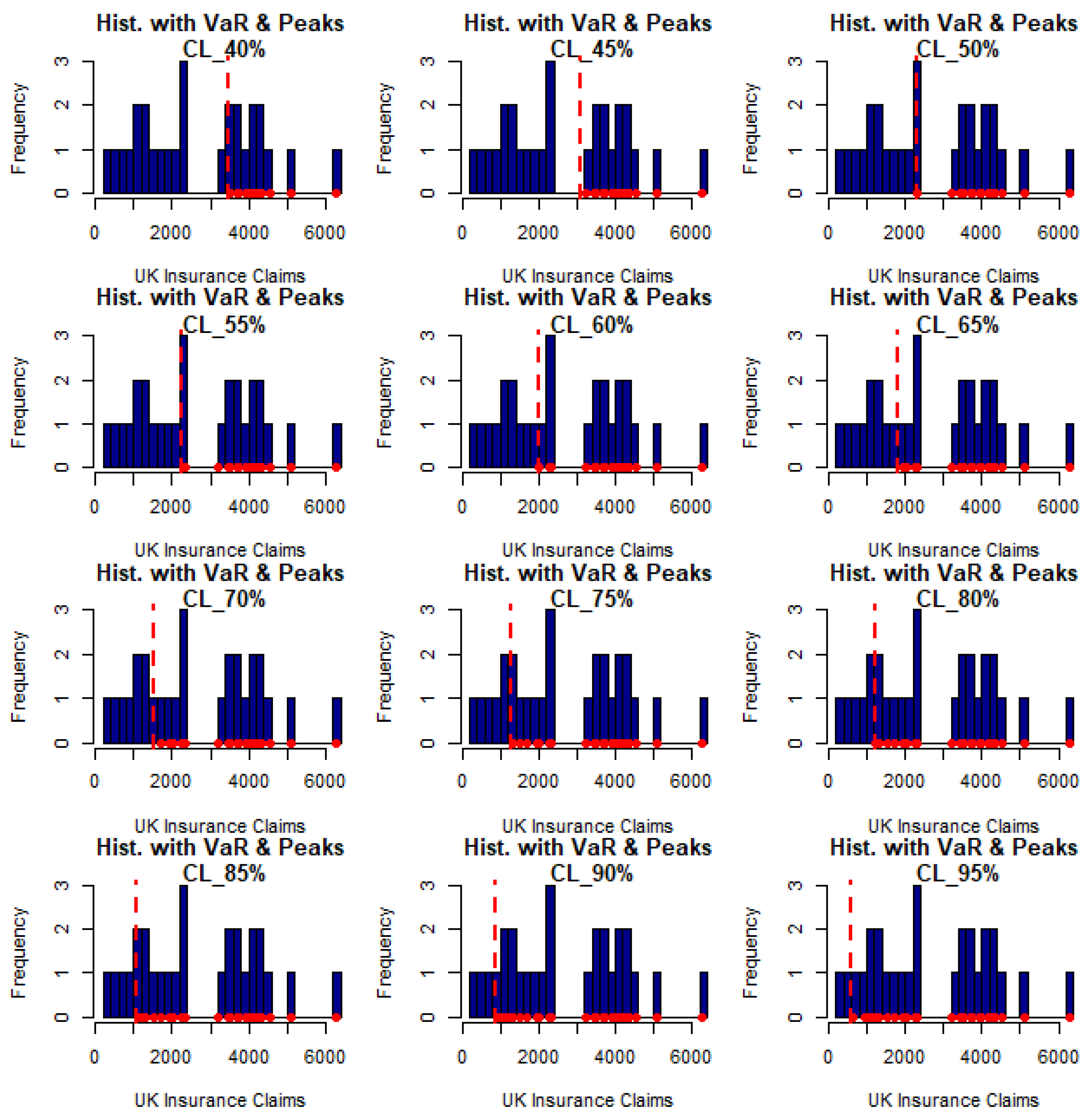
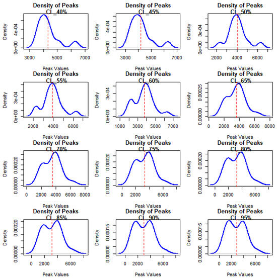
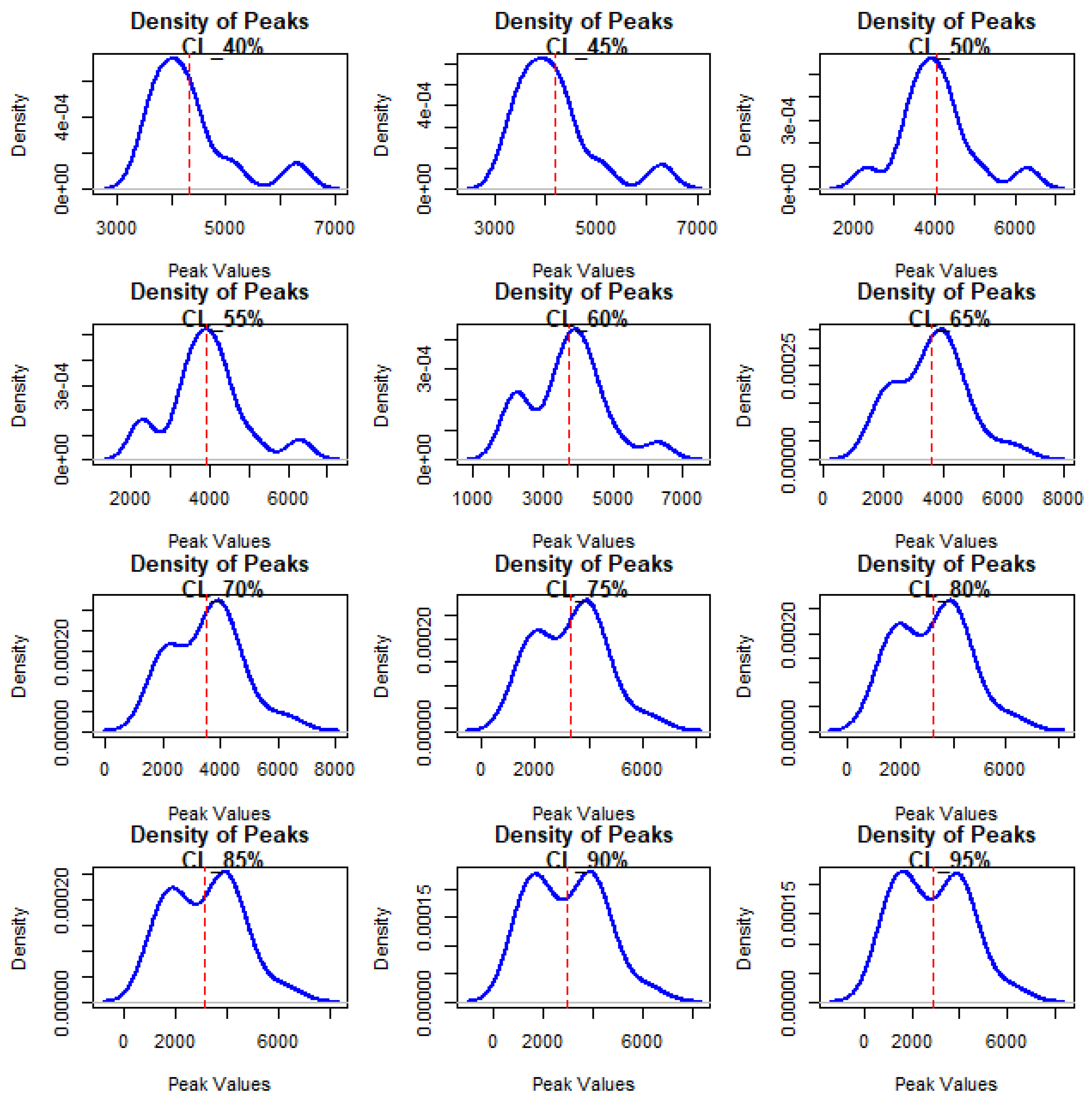
Figure 9 gives the histogram with VaR and peaks analysis under the UK motor non-comprehensive claims triangle data for CL = 40%, 45%, …,95%. Figure 10 provides the density of peaks under the UK motor non-comprehensive claims triangle data for CL = 40%, 45%, …, 95%.

Figure 9. Histogram with VaR and peaks analysis under the UK motor non-comprehensive claims triangle data.

Figure 10. Density of peaks under the UK motor non-comprehensive claims triangle data.

In the UK motor non-comprehensive claims context, TPEX’s superior goodness of fit relative to established exponential families stems from its ability to simultaneously accommodate bimodality (reflecting distinct low- and high-severity claim clusters) and extreme positive skewness driven by rare, large losses. Traditional models either underfit the secondary mode or over-smooth the heavy upper tail, leading to biased tail risk metrics; TPEX’s adaptive decay structure preserves both features without sacrificing parsimony. This translates into more stable and interpretable Value-at-Risk and Tail Mean–Variance estimates across confidence levels, particularly when paired with MLE or Bayesian estimation. The PORT-VaR analysis further confirms that TPEX reliably isolates the high-severity peak cluster, enabling more accurate reserving and capital allocation decisions. Thus, TPEX offers actuaries a flexible yet tractable tool for modeling heterogeneous claim portfolios where tail risk is driven by multimodal loss mechanisms.

6. Economic Case Study Under the Median Values of the USA House Prices Data

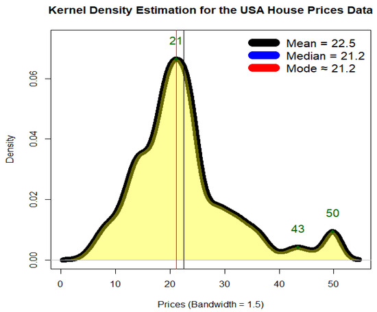
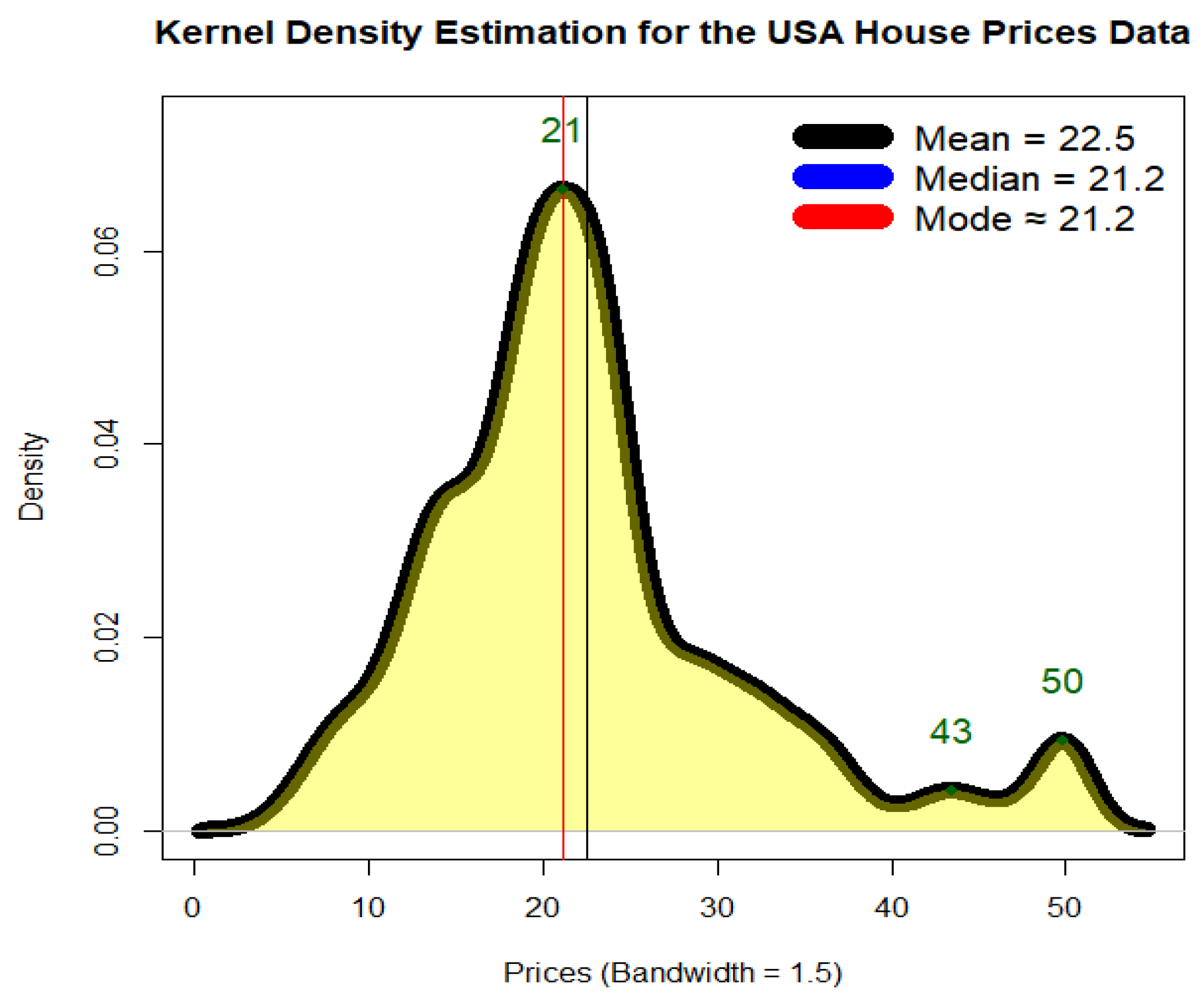
Analyzing the Boston house prices dataset (see AboAlkhair et al. [9]) carries substantial implications for the USA economy, as it enhances our understanding of housing market volatility and broader economic stability. Precise modeling of home prices supports more informed risk evaluations by investors and financial institutions. By employing advanced statistical models, such as the TPEX distribution, analysts can better anticipate extreme price fluctuations, an essential capability for accurately estimating risk measures, like VaR and TVaR, which quantify potential financial losses. These insights are valuable for policymakers seeking to implement preventive measures against housing bubbles. A stable housing market, in turn, bolsters overall economic resilience. Moreover, reliable price forecasts underpin sound mortgage lending practices and effective credit risk management. Enhanced model accuracy also minimizes bias and prediction errors in housing valuations. The Boston dataset comprises median values of owner-occupied home prices (medv) across 506 neighborhoods in the Boston area and has been extensively utilized in real estate economics and econometric research to study and forecast housing price trends. It incorporates a range of socio-economic and environmental predictors, such as crime rates, distance to employment hubs, and air quality, that collectively shape property values. In this study, the dataset serves as a testbed for assessing the performance of the newly proposed TPEX distribution in modeling the tail behavior and extreme values of house prices (for further details, see AboAlkhair et al. [9]). Figure 11 shows the Cullen and Frey plot for the USA Boston house prices data. Based on Figure 11, the empirical data point (represented by the red dot) is in the upper-left region of the plot, indicating that the distribution of house prices exhibits high kurtosis (leptokurtic) and moderate positive skewness. Then, Figure 12 presents the nonparametric kernel density estimate for the USA Boston house prices data. The KDE plot illustrates that the Boston house price data exhibit asymmetry, right-skewness, and bimodality, reinforcing the need for flexible statistical models, like the TPEX distribution, to accurately capture these complex features for risk analysis and forecasting.

Figure 11. The Cullen and Frey plot for the USA Boston house prices data.

Figure 12. The nonparametric kernel density estimation for the USA Boston house prices.

Table 12 presents a parallel risk analysis applied to the USA Boston house prices dataset (specifically, the median owner-occupied home values, medv), again using the same seven estimation methods. It reports the estimated parameters and the corresponding VaR, TVaR, TV, TMV, and EL at 70%, 80%, and 90% confidence levels.

Table 12. Risk analysis under the median values of the USA house prices data.

Method	${\widehat{\mathit{\nu }}}_1$$, {\widehat{\mathit{\nu }}}_2$	VaR (X)	TVaR (X)	TV (X)	TMV (X)	EL (X)
MLE	−7.929211, 0.125143
70%		26	34	65	67	8
80%		29	37	64	70	8
90%		35	43	64	75	8
OrLS	70.249281, 0.004813
70%		28	38	73	74	10
80%		33	42	64	74	9
90%		40	48	54	75	8
WLSQ	26.046314, 0.0083143
70%		28	38	86	81	10
80%		32	42	79	82	10
90%		40	49	71	84	9
CVM	22.47812, 0.008711
70%		29	40	97	88	11
80%		34	44	90	89	10
90%		41	51	82	92	9
Bayes	−7.78383, 0.12549
70%		26	34	65	66	8
80%		29	37	64	69	8
90%		35	43	63	74	8
L-Moment	−8.700577, 0.129732
70%		26	34	61	64	8
80%		29	37	60	67	8
90%		34	42	59	72	8
KE	13.288162, 0.011706
70%		29	40	130	106	12
80%		34	45	127	109	11
90%		42	53	129	117	11

Based on Table 12, we note that the risk measures are much smaller in magnitude compared to the insurance data (e.g., VaR ranges from 26 to 42 vs. thousands in Table 10), consistent with the scale of housing prices versus insurance claim amounts. The MLE, Bayesian, and method of moments yield nearly identical risk estimates across all confidence levels, indicating robustness for this dataset under these methods. OrLS, WLSQ, CVM, and KE produce higher TV and TMV values, especially at the 70% and 80% levels, suggesting that they capture more dispersion in the lower-to-mid tail of the house price distribution. Despite differences in parameter estimates, VaR and TVaR remain relatively stable across methods (e.g., 90% VaR ranges only from 34 to 42), suggesting that extreme quantiles of house prices are less sensitive to estimation method than those in the insurance context.

Table 13 presents a PORT-VaR analysis of the median USA house prices (Boston dataset), revealing how lowering the confidence level from 95% to 40% systematically reduces the VaR threshold while increasing the number of exceedances, from 479 peaks at CL = 95% to 202 at CL = 40%. The peak distributions consistently exhibit right-skewness, with the maximum value fixed at 50.0 (the upper bound of the dataset) across all thresholds, and medians and means steadily rising as CL increases, indicating that higher thresholds isolate more extreme high-end housing values.

Table 13. PORT-VaR analysis under median values of the USA house prices data.

CL	PORT-VaR Results		Peaks Statistics
	VaR	N. of Peaks	Min.; 1st Qu.; Med.; Mean; 3rd Qu.; Max.
40%	22.70	202	22.80 24.23 28.30 30.85 34.85 50.00
45%	22.00	222	22.10 23.73 27.10 30.10 33.38 50.00
50%	21.20	250	21.40 23.10 25.00 29.16 32.85 50.00
55%	20.40	276	20.50 22.60 24.70 28.37 31.77 50.00
60%	19.70	303	19.80 22.00 24.20 27.64 31.05 50.00
65%	19.10	327	19.20 21.45 23.80 27.04 30.10 50.00
70%	18.20	353	18.30 20.80 23.30 26.42 29.60 50.00
75%	17.03	379	17.10 20.25 23.10 25.82 28.70 50.00
80%	15.30	405	15.30 19.70 22.70 25.20 28.20 50.00
85%	13.98	430	14.00 19.30 22.30 24.58 27.50 50.00
90%	12.75	455	12.80 18.70 22.00 23.97 26.65 50.00
95%	10.20	479	10.40 17.85 21.70 23.35 26.30 50.00

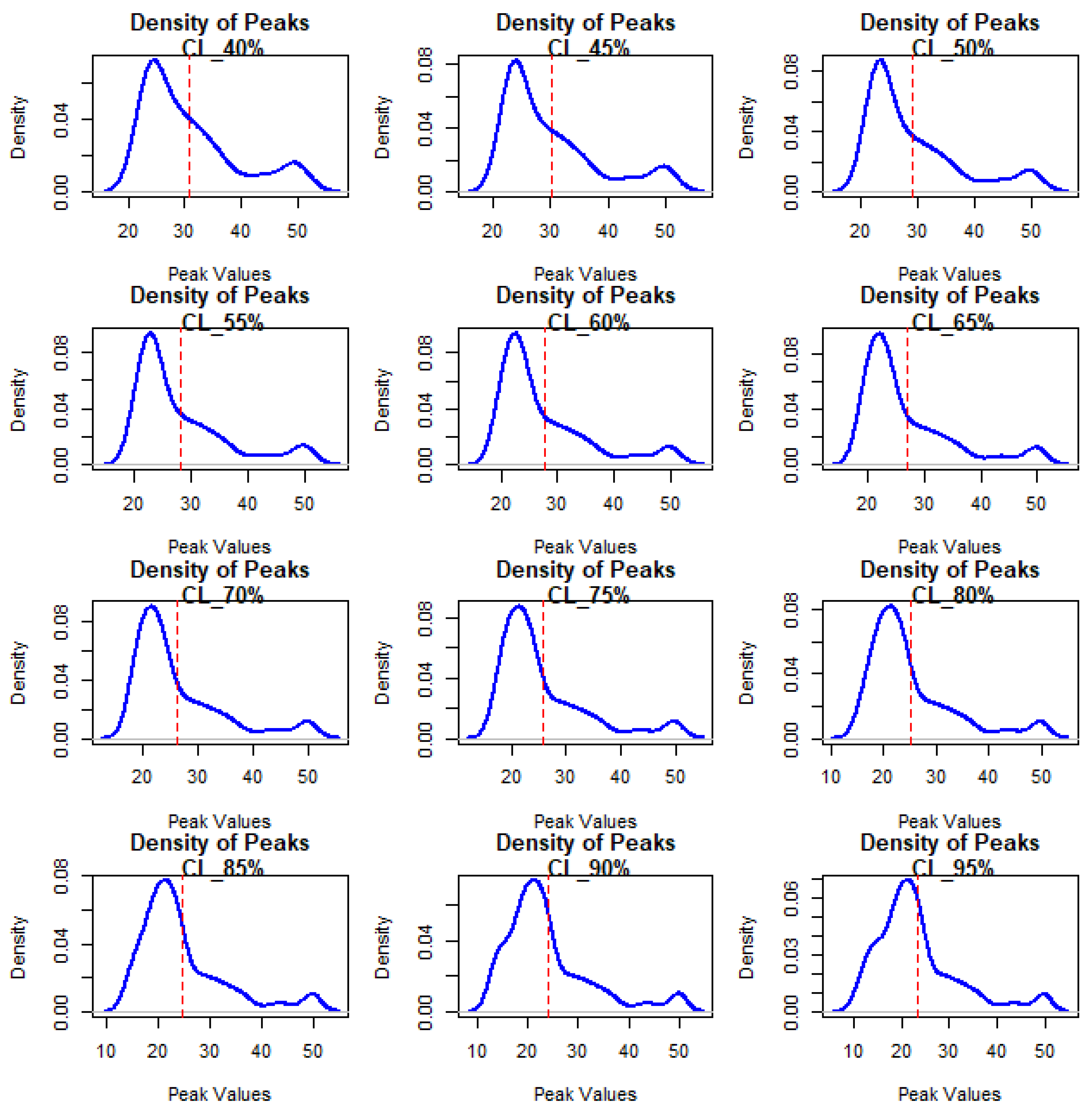
Despite the growing number of peaks at lower CLs, the interquartile range of peaks narrows, reflecting greater concentration in the mid-to-upper price segment under stricter thresholds. This behavior aligns with the bimodal, right-skewed structure observed in Figure 11 and Figure 12, where a secondary cluster near the upper tail (around 40–50) drives tail risk. The stability of the maximum (50.0) and the gradual decline in peak minima confirm the presence of a bounded but heavy upper tail, typical of real estate valuation data.

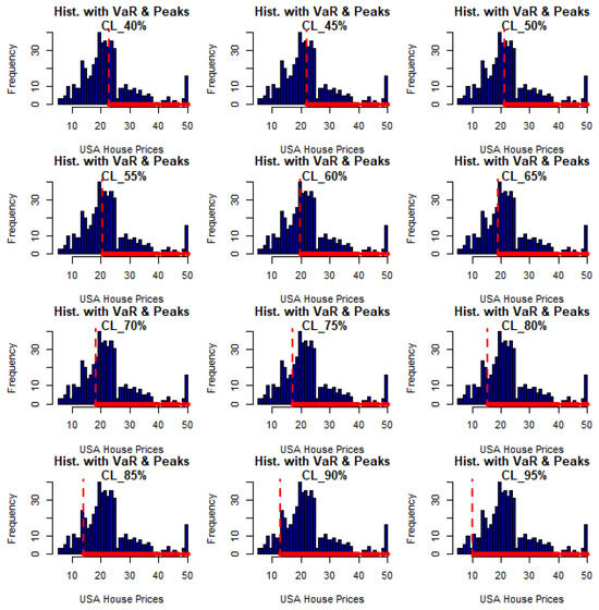
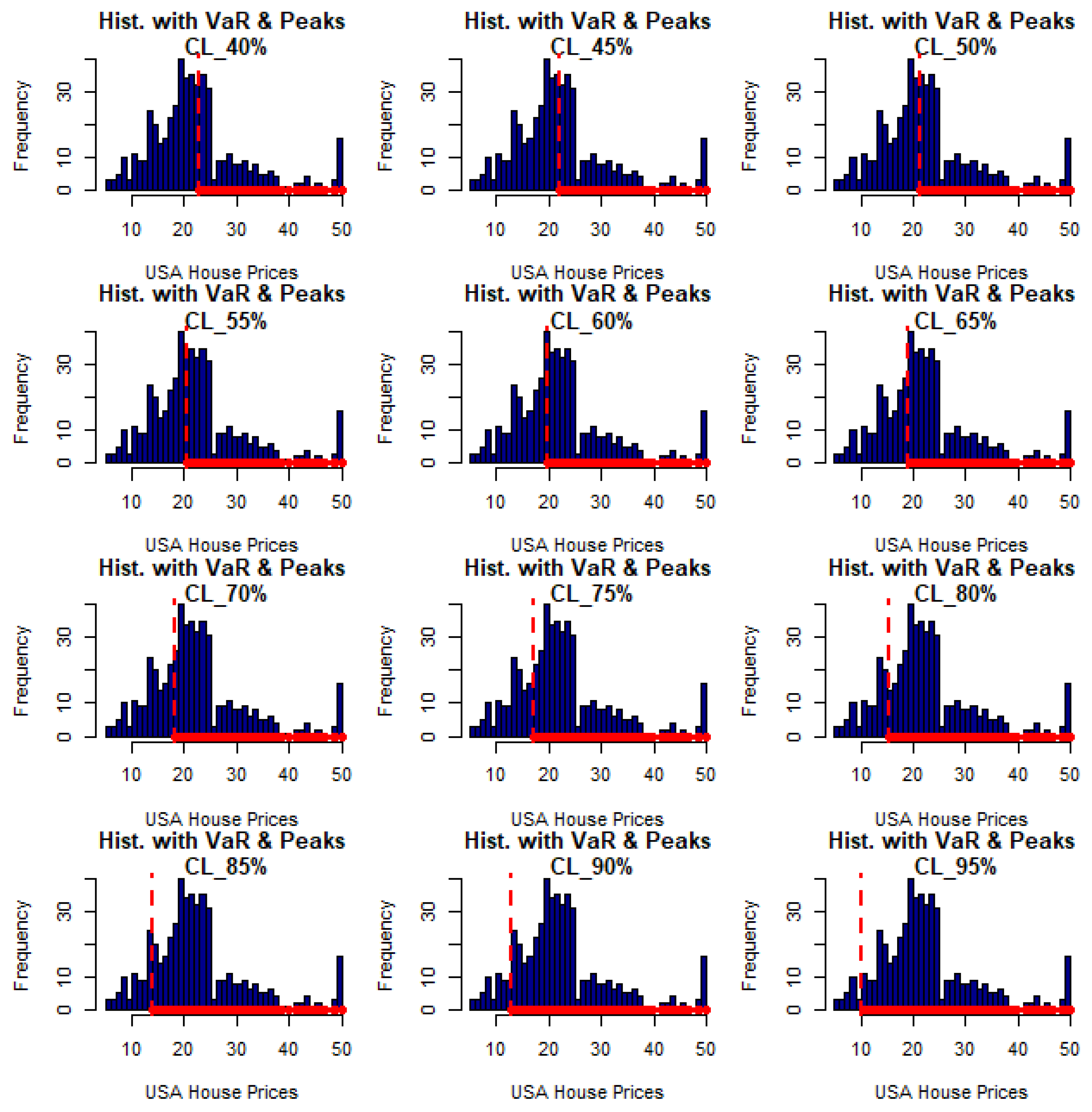
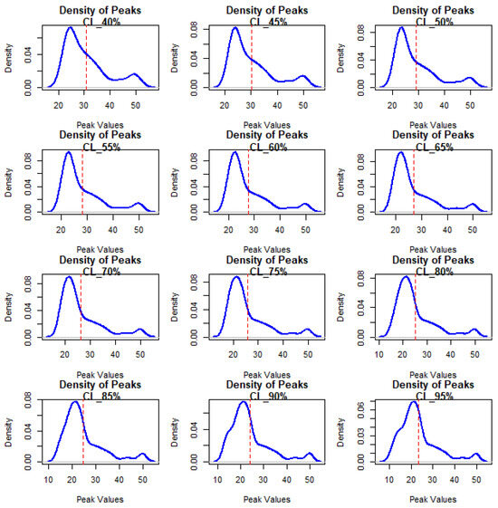
Figure 13 gives the histogram with VaR and peaks analysis under the median values of the USA house prices data for CL = 40%, 45%, …, 95%. Figure 14 provides the density of peaks under the median values of the USA house prices data for CL = 40%, 45%, …, 95%.

Figure 13. Histogram with VaR and peaks analysis under the median values of the USA house prices data.

Figure 14. Density of peaks under the median values of the USA house prices data.

For the Boston housing data, TPEX’s competitive performance arises from its capacity to model leptokurtic, right-skewed price distributions with a bounded upper tail, a pattern that symmetric or light-tailed exponential extensions cannot replicate without distortion. The model’s state-dependent decay rate accommodates the concentration of neighborhoods in the mid-price range while still capturing the secondary cluster near the market ceiling, reflecting genuine economic segmentation rather than a statistical artifact. This structural fidelity yields more robust extreme-value forecasts and tail risk indicators, critical for mortgage lending, portfolio stress testing, and policy design aimed at housing market stability. Unlike competing distributions that either truncate the upper tail or overestimate tail thickness, TPEX balances flexibility with exponential-like asymptotics, ensuring finite moments and interpretable risk metrics. The results affirm TPEX as a practical choice for econometric applications where price dynamics exhibit asymmetric clustering and bounded extremes.

7. Conclusions

This paper introduced a novel two-parameter exponential (TPEX) distribution and comprehensively investigated its theoretical properties, estimation methods, and two real applications in risk analysis. A large-scale simulation study was conducted to evaluate seven estimation techniques including the maximum likelihood estimation (MLE), ordinary least squares (OrLS), Cramér–von Mises (CVM), weighted least squares (WLS), L-moments, Kolmogorov–Smirnov (KE), and Bayesian estimation using mean squared error as the primary criterion. The results showed that the MLE and Bayesian methods mostly provided parameter estimates that were close to the initial values. The model was then applied to four real datasets: two biomedical datasets (relief times and guinea pig survival times) were used to compare estimation methods, while UK motor non-comprehensive insurance claims and US Boston house prices served as case studies for model comparison and risk assessment. Goodness-of-fit indicators, including AIC, BIC, CVM, Anderson–Darling, and KS statistics, confirmed the TPEX model’s superior performance over ten competing exponential-based distributions. Furthermore, PORT-VaR analyses revealed how tail behavior and risk indicators (VaR, TVaR, TV, TMV, EL) varied across confidence levels and estimation strategies, highlighting the sensitivity of risk quantification to methodological choices. Finally, two case studies under the peaks over random threshold analysis are presented with all details.

This study acknowledges several limitations that contextualize its findings. First, the empirical validation relies on four real-world datasets from biomedical, insurance, and real estate domains, which may limit generalizability to other sectors or data-generating processes. Second, the Monte Carlo simulation evaluates only three parameter configurations and a restricted range of sample sizes, potentially omitting estimator performance under extreme skewness or high-dimensional settings. Third, the framework assumes independent and identically distributed observations, excluding temporal dependencies, spatial correlations, or covariate-driven heterogeneity common in longitudinal actuarial data. Additionally, the PORT-VaR analysis employs static confidence thresholds without incorporating dynamic stress testing or regime-switching mechanisms. Finally, while seven estimators are compared, hybrid or machine learning-enhanced inference methods remain unexplored.

Future research should extend the TPEX framework into regression and multivariate formulations to accommodate covariate effects and interdependent risk factors in complex portfolios. Incorporating adaptive threshold selection, Bayesian updating, or regime-switching PORT-VaR could enhance tail risk forecasting under structural breaks. Developing hybrid estimation pipelines that integrate MCMC with gradient-based or machine learning optimizers may improve computational scalability. Finally, validating the model on emerging risk domains such as climate-related losses, cyber incidents, or digital asset markets would assess its robustness in non-stationary, high-frequency environments.

While the proposed distribution is characterized by a relatively light-tailed structure, its practical applicability for actuarial risk assessment has been empirically substantiated across the examined datasets. This does not imply universal optimality; rather, it establishes the model as a reliable and contextually appropriate alternative that demonstrates competitive performance in targeted risk modeling scenarios.

8. Discussion

The central finding of this article is that the proposed TPEX distribution offers a demonstrably superior alternative to established exponential-type models for modeling complex, real-world risk data. Across biomedical, actuarial, and economic contexts, TPEX consistently outperforms ten competing distributions, primarily due to its unique ability to capture pronounced skewness, bimodality, and heterogeneous tail behavior while maintaining analytical tractability. Rather than imposing restrictive shape constraints, like conventional exponential extensions, TPEX incorporates a state-dependent decay rate and a quadratic vanishing density at the origin. This mathematical structure allows it to adapt seamlessly to diverse empirical patterns—from the zero-initial-hazard survival profiles in biomedical data to the heavy-tailed, dual-cluster claim distributions in UK motor insurance and the leptokurtic, right-skewed housing price data in the US market. Comprehensive goodness-of-fit metrics (AIC, BIC, AD, CVM, and KS) consistently rank TPEX highest across all four applications, confirming that its parametric flexibility directly translates to more accurate empirical representation without sacrificing parsimony.

The model’s practical utility is further reinforced by the stability and reliability of its parameter recovery. Extensive MCMC simulations demonstrate that maximum likelihood and Bayesian estimators consistently yield the lowest mean squared errors and most reliable convergence across varying sample sizes and parameter configurations. When applied to real-world datasets, these two methods produce nearly identical risk indicators, underscoring a methodological robustness that practitioners can trust. In contrast, alternative estimators (e.g., L-moments, Kolmogorov, or least-squares variants) tend to introduce greater variability in tail risk measures, highlighting that estimator selection is as critical as model choice. Crucially, TPEX proves highly effective in extreme-value analysis under the PORT-VaR framework. The model accurately quantifies key risk indicators (VaR, TVaR, Tail Variance, TMV, and the corresponding expected loss) across multiple confidence levels, capturing the distinct high-severity clusters that drive tail risk in both insurance claims and real estate markets. The analysis also reveals that while risk estimates are sensitive to the estimation technique employed, pairing TPEX with MLE or Bayesian inference delivers stable, interpretable, and financially meaningful tail risk metrics.

Ultimately, TPEX is not merely a theoretical extension but a practically validated instrument that bridges mathematical flexibility with actuarial and economic relevance. Its consistent dominance across heterogeneous datasets, coupled with robust estimation protocols and reliable PORT-VaR performance, establishes it as a preferable choice for modeling asymmetric, tail-driven phenomena where underestimating extreme losses can have severe financial or operational consequences. While future research should explore multivariate formulations, covariate integration, and dynamic thresholding, the current evidence strongly supports TPEX as a reliable, empirically grounded distribution for contemporary risk assessment, insurance reserving, market volatility forecasting, and strategic decision-making under uncertainty.

References

- Tahir, M.H.; Hussain, M.A.; Cordeiro, G.M.; El-Morshedy, M.; Eliwa, M.S. A new Kumaraswamy generalized family of distributions with properties, applications, and bivariate extension. Mathematics 2020, 8, 1989. [Google Scholar] [CrossRef] [Scilit]
- Gupta, R.D.; Kundu, D. A new class of weighted exponential distributions. Statistics 2009, 43, 621–634. [Google Scholar] [CrossRef] [Scilit]
- Li, N.; Lei, Y.; Lin, J.; Ding, S.X. An improved exponential model for predicting remaining useful life of rolling element bearings. IEEE Trans. Ind. Electron. 2015, 62, 7762–7773. [Google Scholar] [CrossRef] [Scilit]
- Sun, M.; Guo, K.; Zhang, D.; Yang, B.; Sun, J.; Li, D.; Huang, T. A novel exponential model for tool remaining useful life prediction. J. Manuf. Syst. 2024, 73, 223–240. [Google Scholar] [CrossRef] [Scilit]
- Gross, J.; Clark, V.A. Survival Distributions: Reliability Applications in the Biometrical Sciences; John Wiley: New York, NY, USA, 1975. [Google Scholar]
- Charpentier, A. (Ed.) Computational Actuarial Science with R.; CRC Press: Boca Raton, FL, USA, 2014. [Google Scholar]
- Bjerkedal, T. Acquisition of resistance in Guinea pigs infected with different doses of virulent tubercle bacilli. Am. J. Hyg. 1960, 72, 130–148. [Google Scholar] [PubMed]
- Mohamed, H.S.; Cordeiro, G.M.; Minkah, R.; Yousof, H.M.; Ibrahim, M. A Size-of-Loss Model for the Negatively Skewed Insurance Claims Data: Applications, Risk Analysis Using Different Methods and Statistical Forecasting. J. Appl. Stat. 2024, 51, 348–369. [Google Scholar] [CrossRef] [Scilit] [PubMed]
- AboAlkhair, A.M.; Al-Nefaie, A.H.; Ibrahim, M.; Hashim, M.; Aljadani, A.; Mansour, M.M.; Roushdy, N.; Ahmed, N.A.; Yousof, H.M.; Ahmed, B. The Burr Inverse Weibull Model for Risk Analysis Under US Social Security Administration Disability Data Using Peaks Over Random Threshold Method with a Case Study in KSA. Pak. J. Stat. Oper. Res. 2025, 21, 447–474. [Google Scholar] [CrossRef] [Scilit]
Disclaimer/Publisher’s Note: The statements, opinions and data contained in all publications are solely those of the individual author(s) and contributor(s) and not of MDPI and/or the editor(s). MDPI and/or the editor(s) disclaim responsibility for any injury to people or property resulting from any ideas, methods, instructions or products referred to in the content. |
© 2026 by the authors. Licensee MDPI, Basel, Switzerland. This article is an open access article distributed under the terms and conditions of the Creative Commons Attribution (CC BY) license.