Analysis of a Hybrid System Comprising Four Series-Connected Subsystems Using Reduction Techniques and Copula-Based Modeling

Abstract

Wireless Sensor Networks (WSNs) deployed in agricultural and industrial environments require high reliability to ensure continuous monitoring and data transmission. This study presents a reliability analysis of a hybrid WSN system comprising four series-connected subsystems: (1) the central processing unit, (2) sensor nodes in cluster A, (3) sensor nodes in cluster B, and (4) communication relay units. The system operates under a k-out-of-n: G mechanism, where subsystems 2 and 3 require at least one operational unit, while subsystem 4 requires at least two. Whereas unit failures follow exponential distributions, repair processes are modeled using either general distributions or Gumbel–Hougaard copula-based approaches to capture dependencies among multiple repair units. Using Laplace transforms and supplementary variable techniques, we evaluate system reliability metrics and demonstrate that copula-based repair strategies significantly improve availability and the expected profit function. Furthermore, we propose a reduction technique governed by a factor $\rho$ that decreases component failure rates, thereby enhancing overall system reliability relative to the baseline configuration.

1. Introduction

Contemporary engineering systems increasingly operate in settings where continuous-time degradation processes interact with discrete failure and repair events, giving rise to what are commonly referred to as hybrid systems in reliability engineering. A hybrid system is characterized not by a particular application domain, but by the coexistence and interplay of stochastic degradation, random failures, and stochastic maintenance operations within a unified modeling framework. The defining feature of such systems is that their dependability cannot be adequately captured by either purely continuous degradation models or purely discrete failure models; it is precisely the interaction between these coupled stochastic processes, further complicated by statistically interdependent repair operations, that renders hybrid systems both analytically challenging and practically significant. Such systems are prevalent in modern networked and cyber–physical infrastructures, where the demand for uninterrupted operation demands rigorous and comprehensive reliability modeling frameworks.

A key structural characteristic that defines the class of hybrid systems studied in this paper is the presence of redundancy mechanisms, most naturally represented through k-out-of-n: G configurations and series–parallel topologies. In a k-out-of-n: G scheme, the system remains operational as long as at least k out of its n constituent units are functioning; failure of more than n–k units results in complete system breakdown. This configuration finds broad applicability across transmission relay systems, energy distribution networks, power plant infrastructures, and quality control systems. When embedded within a series–parallel architecture, in which subsystems are connected sequentially while individual units within each subsystem operate in parallel, the resulting structure captures a realistic balance between fault tolerance and operational dependency. This structural combination motivates the reliability model proposed in this paper: a four-subsystem series–parallel hybrid system in which Subsystems 2 and 3 each require at least one operational unit (1-out-of-3), Subsystem 4 requires at least two (2-out-of-4), and Subsystem 1 constitutes a single critical unit (1-out-of-1). Failure rates across all subsystems are assumed to follow exponential distributions, while repair processes are modeled through both general distributions and copula-based approaches to capture statistical interdependence among repair durations.

Inspired by this cohesive structural viewpoint, WSNs and serial–parallel computer networks serve throughout this paper as illustrative deployment contexts rather than standalone case studies. Both system types naturally exhibit the hybrid characteristics described above, making them well-suited exemplars for the proposed modeling framework. In WSNs, sensor nodes undergo progressive performance deterioration such as energy depletion or environmental stress alongside abrupt failures and repair interventions. Network functionality is preserved as long as a sufficient number of sensor nodes remain operational within each cluster, a condition well captured by K-out-of-n models. Similarly, serial–parallel computer networks rely on combinations of series and parallel subsystems to enhance fault tolerance, with overall functionality depending jointly on the durability of individual components and the logical architecture of the network. Despite originating from different application domains, both system types share the same key dependability—characteristics redundancy-driven fault tolerance, stochastic degradation, and maintenance interdependence—that the proposed model is specifically designed to address. Numerous researchers have contributed to evaluating the performance of such systems. Catelani et al. [1] investigated the effects of node deployment and redundancy on the dependability of WSNs operating in challenging environments. Jesus et al. [2] evaluated the reliability of a wireless visual sensor network by integrating Markov modeling with fault tree analysis. Lechang et al. [3] assessed the reliability of reconfigurable multi-stage systems using a graph-based path-searching approach. Singh et al. [4] examined copula-based repair methods that predict the performance of two-unit systems. Elshoubary et al. [5,6] employed copula-based methods to assess the effectiveness of reduction methodologies on complex systems including the Kafka platform and water bottling systems. We mention some relevant works that collectively lay the theoretical and applied foundations on which the current study is based. According to [7], WSNs face a number of difficult and perhaps dangerous situations; for example, as they are often used outdoors, WSNs face challenges from extreme weather that can degrade electrical performance. Oszczypa et al. [8] proposed a combined Markov Chain and Monte Carlo simulation approach to optimize the number of components in a k-out-of-n system, where the minimum number of required components is treated as a random variable, with the goal of maximizing availability while minimizing costs; the approach was validated on real transport systems. Ogura et al. [9] proposed an optimization framework for system reliability under cost constraints, demonstrating that power-type cost functions yield the best performance results. Kumar et al. [10] developed a continuous time Markov process model to analyze key reliability metrics—including $MTTF$, component-wise reliability, and sensitivity indices—across a WSN’s core components, with the aim of supporting the design of more robust WSN systems. Zhao et al. [11] employed a Continuous-Time Markov Chain combined with Monte Carlo simulation to optimize the number of components in a k-out-of-n redundancy structure, with the objective of achieving a target availability level at minimum cost under dynamically changing operating conditions. Addabbo et al. [12] analyzed and compared the reliability and availability of several linear sensor network architectures. Because it shows how likely it is that a system or part will work the way it is supposed to under certain conditions for a set amount of time, reliability is essential in many industrial and manufacturing areas. There are many ways to assess a complex system’s reliability. Reordered, reliability forecasting is widely adopted technique for calculating the failure rates of electronic components [13,14]. The Reliability Block Diagram is another method for assessing the overall reliability of the system [15]. Using Boolean logic to model and evaluate contributing lower-level events leading to an undesired system condition, Fault Tree Analysis is a top-down, deductive method for examining an undesirable system condition [16,17]. Ciani et al. [18] employed a mix of event tree analysis and fuzzy fault tree analysis to evaluate the dependability of hybrid systems used in advanced treatment units for the reuse of industrial wastewater. Gokdere et al. [19] used the transition matrix approach to analyze a time-dependent system. Dhruv Raghav et al. [20] examined a complex system comprising two series-connected subsystems, where the first subsystem adhered to the 2-out-of-5: G scheme, while the second subsystem operated under a 1-out-of-2: G policy, considering multiple failure modes and copula repair strategies. Ibrahim Yusuf et al. [21] assessed the dependability of a communication network system that had a redundant relay station in both partial and complete failure scenarios. Niaki and Yaghoubi [22] developed closed-form expressions to predict the reliability function and Mean Time To Failure ($MTTF$) of a 1-out-of-n cold standby system using the Markov approach.

Despite the breadth of existing work, several important gaps remain in the reliability literature for hybrid systems of this class. First, the most existing models rely on Reliability Block Diagrams or Fault Tree Analysis in isolation, assume subsystem independence and statistically independent repair durations. This assumption is frequently violated in practice, where repair times across multiple failed units are often correlated due to shared maintenance resources, uniform repair protocols, or common environmental stressors. Second, relatively few studies have simultaneously addressed structural redundancy, dependent repair modeling, and component-level failure rate optimization within a single unified framework. Third, the application of copula functions—which offer a flexible and mathematically rigorous mechanism for modeling repair dependencies—remains underexplored multi-subsystem series–parallel systems with mixed k-out-of-n configurations. The present study is motivated by these gaps and aims to provide a comprehensive reliability modeling framework that addresses all three dimensions within a cohesive analytical approach.

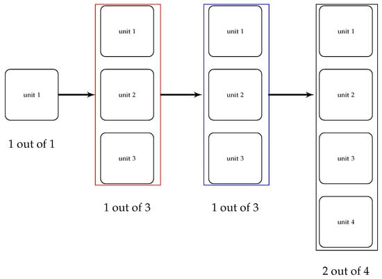
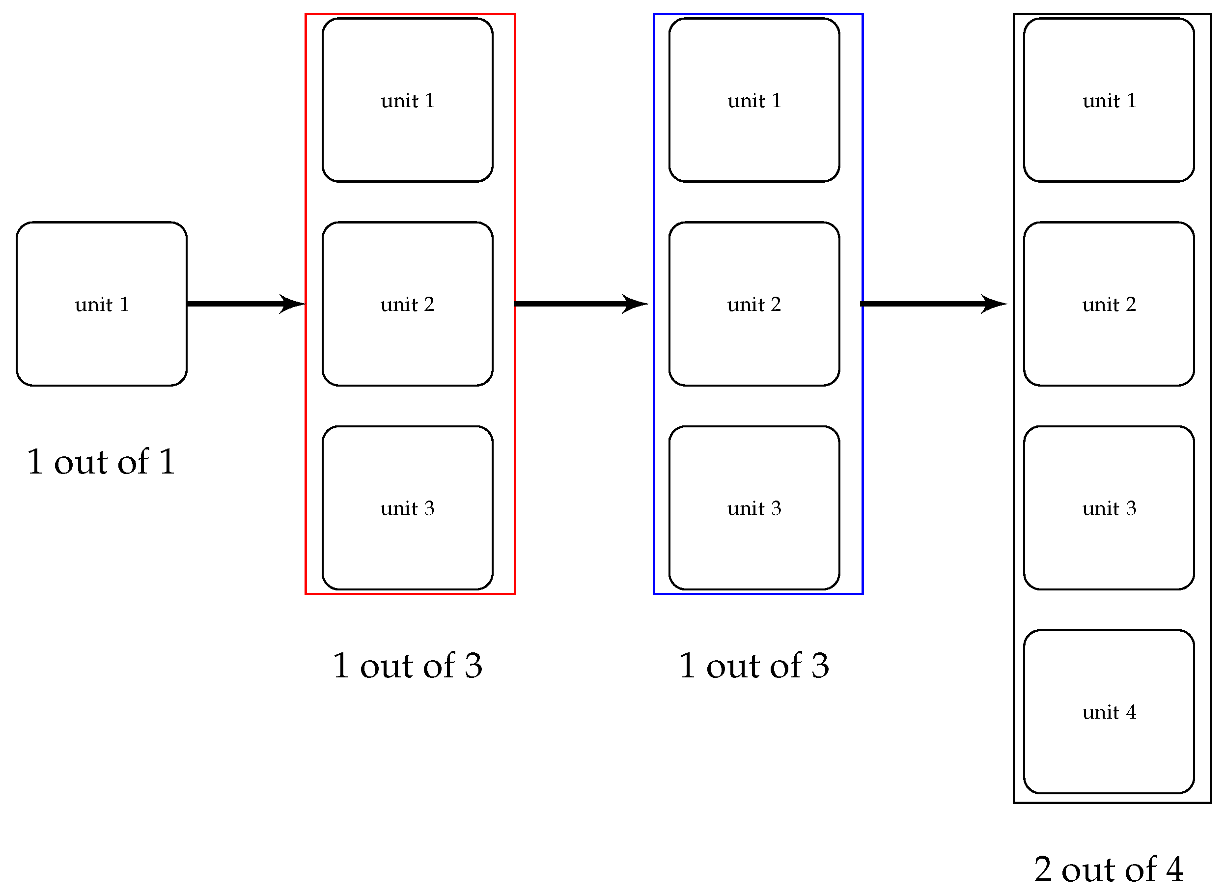
This paper makes three primary contributions to the reliability modeling literature. First, it presents a unified four-subsystem reliability model that integrates Reliability Block Diagram and Fault Tree Analysis perspectives to encompass both series–parallel configurations and logical failure interdependencies (Figure 1). Second, it incorporates repair modeling through the Gumbel–Hougaard copula family, which provides a flexible mathematical framework that differs structurally from conventional independent repair models, even at its independence boundary, and can capture positive dependence when extended in multi-unit systems. Third, it introduces and evaluates a reduction technique governed by a factor $\rho$∈ (0, 1) that systematically decreases component failure rates, providing a quantitative basis for investment decisions regarding component quality improvement. Using Laplace transforms and supplementary variable techniques, the paper evaluates system availability, reliability, mean time to failure ($MTTF$), sensitivity indices, and expected profit across three scenarios: copula-based repair, general distribution repair, and reduction method. The remainder of the paper is organized as follows. Section 2 describes the system model, its assumptions, state definitions, and notational conventions. Section 3 develops the mathematical model via transition graphs and a system of partial differential equations. Section 4 presents a numerical analysis of system performance indicators across the three scenarios. Section 5 summarizes the key findings, practical implications, and directions for future research.

Figure 1. Block diagram of the hybrid WSN system showing four subsystems: central gateway (1-out-of-1), two sensor clusters (each 1-out-of-3), and relay network (2-out-of-4).

We recognize that simply listing prior studies without explicitly identifying their shared shortcomings represents a missed opportunity. We have now added a dedicated paragraph in the Introduction that consolidates the following recurring limitations found across the cited literature:

(a) Independence assumption in repairs: The overwhelming majority of existing reliability models for series–parallel and k-out-of-n systems—including those of Raghav et al. [20], Singh et al. [4], and Yusuf et al. [21]—assume that repair processes for individual failed units are statistically independent. This is unrealistic in practice, where shared maintenance crews, common spare part inventories, or synchronized environmental recovery inherently couple repair durations.

(b) Limited subsystem scope: Most prior works analyze systems comprising at most two subsystems (e.g., [4,20]), which is insufficient to capture the layered architecture of modern WSNs comprising gateway, sensing, relay, and power subsystems simultaneously.

(c) Uniform k-out-of-n policy: Existing models typically apply a single k-out-of-n configuration uniformly across all subsystems. The present model, by contrast, employs heterogeneous redundancy levels (1-out-of-1, 1-out-of-3, 1-out-of-3, and 2-out-of-4) that reflect the distinct criticality of each WSN layer.

(d) Absence of failure rate reduction strategies: None of the directly comparable studies (e.g., [4,19,20,21,22]) incorporates a systematic component-quality improvement mechanism. Our reduction technique (factor $\rho$) addresses this gap, providing a quantifiable means of investing in component reliability.

(e) Environmental failure rate: The role of ${\lambda }_5$ as a shared environmental stressor affecting all subsystems simultaneously is largely absent from prior models, representing a further gap that the present work addresses.

Research Objectives, Assumptions, and Main Contributions

This study aims to develop a comprehensive reliability modeling framework for a complex system comprising four interrelated subsystems, explicitly accounting for both structural dependencies and repair-time interdependencies. The proposed model addresses limitations in existing research, which predominantly relies on Reliability Block Diagrams or Fault Tree Analysis under the simplifying assumptions of subsystem independence and mutually independent repairs.

The proposed methodology assumes that the failure logic of each subsystem can be effectively represented through a unified Reliability Block Diagram–Fault Tree Analysis framework, while repair durations associated with various failure modes may exhibit statistical interdependence due to shared maintenance resources, environmental factors, or synchronized repair protocols. The system is presumed to function in steady-state conditions, with well-defined failure distributions and clearly specified repair procedures.

This paper makes three primary contributions. First, it presents a unified four-subsystem reliability model that integrates Reliability Block Diagram and Fault Tree Analysis to capture both series–parallel configurations and logical failure interdependencies. Second, it incorporates dependent repair modeling through a copula-based framework, enabling a more accurate representation of real-world maintenance operations. Third, the framework provides a transparent and flexible approach for evaluating system-level dependability while preserving explicit physical interpretation at the subsystem level.

2. Description of the Model and Its Notations

2.1. Overview of the States

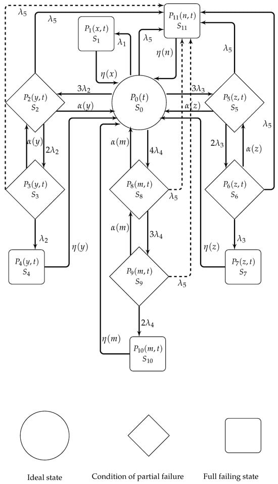
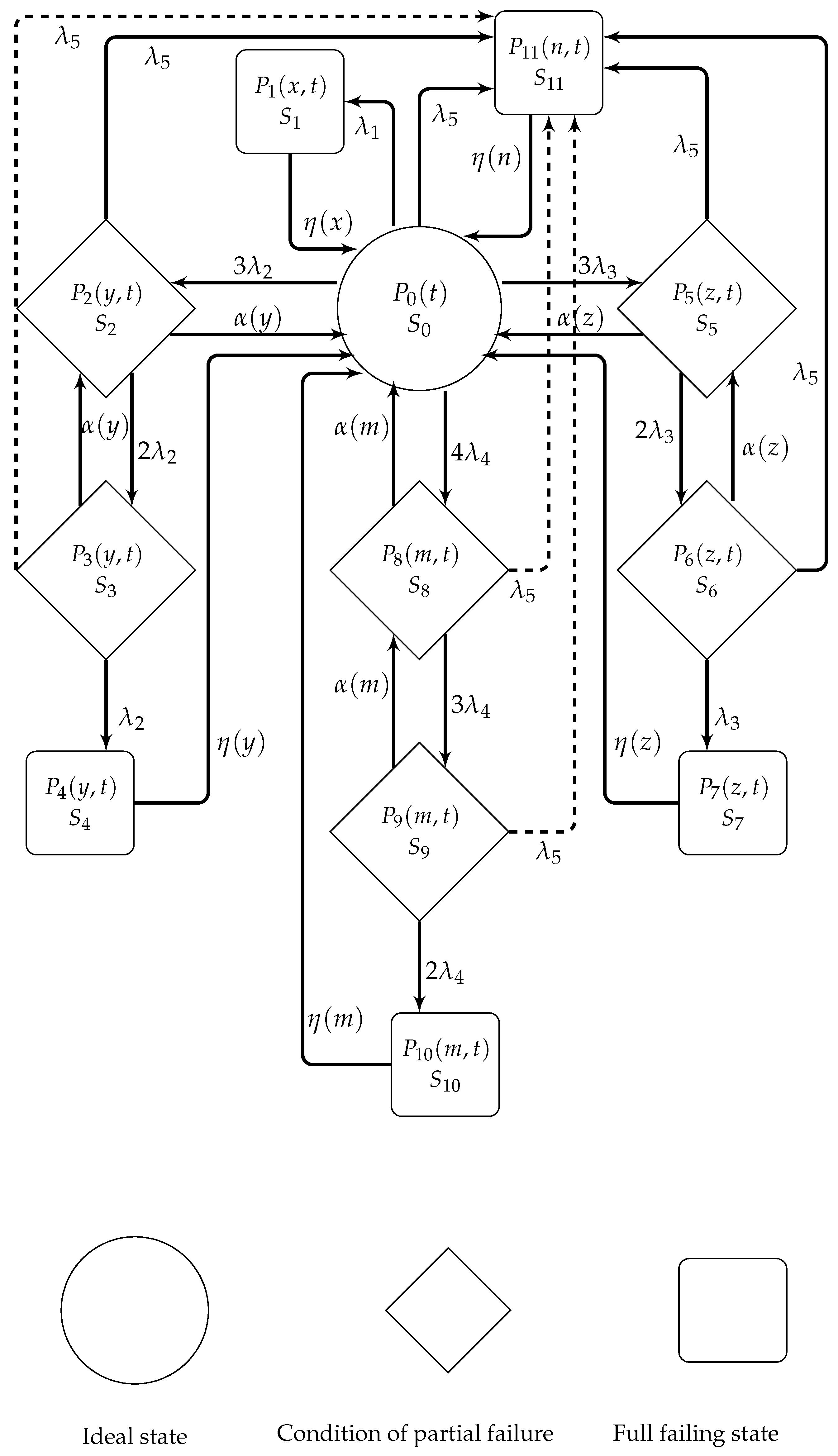
Table 1 summarizes the various possible states that the system can occupy. $S_0$, $S_2$, $S_3$, $S_5$, $S_6$, $S_8$, and $S_9$ are categorized as active (operational or degraded), whereas $S_1$, $S_4$, $S_7$, $S_{10}$, and $S_{11}$ are classified as inactive (complete failure). $S_0$ denotes the fully operational initial state, in which all components function without fault, as illustrated in Figure 2. States $S_2$, $S_3$, $S_5$, $S_6$, $S_8$, and $S_9$ represent progressive levels of degradation or partial failure resulting from the failure of one or two units within subsystems 2, 3, or 4, respectively. State $S_1$ corresponds to complete system failure due to the failure of subsystem 1. States $S_4$, $S_7$, $S_{10}$, and $S_{11}$ represent complete failure caused by the failure of more than two units within subsystems 2, 3, or 4, with repair governed by the Gumbel–Hougaard copula distribution.

Table 1. Description of all system states ($S_0$–$S_{11}$), including fully operating, degraded (small or major partial failure with ongoing repair), and wholly failed (subject to copula-based or comprehensive repair), subsystems involved, and repair approach.

State	Description
$S_0$	Fully Operational State: With every component working well and without flaws, the system is running at maximum efficiency.
$S_2$, $S_3$, $S_5$, $S_6$, $S_8$, $S_9$	Degraded (Active) States: The system remains operational, as the k-out-of-n redundancy criteria are still met; however, one or more individual units within subsystems 2, 3, or 4 have failed and are in the process of repair. These phases indicate partial failure with ongoing system functionality, rather than total collapse.
$S_1$, $S_4$, $S_7$, $S_{10}$, $S_{11}$	Complete Failure (Inactive) States: The system has become inoperative. States $S_4$, $S_7$, and $S_{10}$ occur when the count of failed units in subsystems 2, 3, or 4 surpasses the k-out-of-n threshold; States $S_1$ and $S_{11}$ represent the total failure of subsystem 1 or a complete failure induced by environmental factors, respectively. The repair process in these states is shown using the Gumbel–Hougaard copula.

Figure 2. The state transition diagram of the Markov model, illustrating the transitions between the fully functioning state ($S_0$), partial failure states ($S_2,S_3,S_5,S_6,S_8,S_9$), and complete failure states ($S_1,S_4,S_7,S_{10},S_{11}$).

2.2. Assumptions

We assumed the following when creating the model:

• Initially, every subsystem runs flawlessly.
• As seen in Figure 1, the system is made up of four series–parallel subsystems. One unit set up in a 1-out-of-1 configuration makes up Subsystem 1. Three similar units coupled in a 1-out-of-3 configuration comprise Subsystem 2. Likewise, Subsystem 3 comprises three units operating in a one-out-of-three configuration. Four identical parts arranged in a 2-out-of-4 pattern make up Subsystem 4.
• Once a failed unit is in a non-operational state, it can be repaired.
• The copula repair is triggered when a unit in the subsystem completely fails.
• It is assumed that after a copula repair, the system would operate as if it had never been damaged and that no problems will arise.
• Immediately after repair, the unit is capable of performing its assigned duty.

2.3. Notation

t/s: Time variable/Laplace transform variable.

${\lambda }_1$/${\lambda }_2$: Failure rates associated with each subsystem 1 and subsystem 2 unit.

${\lambda }_3$/${\lambda }_4$: Failure rates of individual units for subsystems 3 and 4.

${\lambda }_5$: Environmental failure rate (temperature spikes, humidity, rain, or dust).

$\sigma \left(x\right)$: The repair rates for subsystems 1, 2, 3, and 4 that match their levels of partial failure.

$P_0\left(t\right)$: Scalar probability of the system being in the fully operational state $S_0$ at time t.

$\stackrel{*}{P}\left(s\right)$: The Laplace transform is a useful tool to analyze the probability of transitions between states within a system over time.

$P_i(\zeta ,t)$: Probability density function for states involving ongoing repair, where $\zeta \in \{x,y,z,m,n\}$ denotes the elapsed repair time (age variable).

$C_1$/$C_2$: Revenue/The cost needed for system upkeep and operation.

$E_p\left(t\right)$: The anticipated profit as a result of the system’s operation over the time period $[0,t]$.

$\nu \left(x\right)$: A formula that measures the combined likelihood of moving from state $S_j$ (failed) to state $S_0$ (successful) for i = 1, 4, 7, 10, 11.

$P_{up}\left(t\right)$: System availability at time t (probability system is operational).

$R\left(t\right)$: System reliability at time t (probability of failure-free operation).

$MTTF$: Mean Time To Failure (expected operating time before first failure).

2.4. Mapping of Subsystems to Real-World Wireless Sensor Network Architecture

This subsection maps each of the four subsystems to the corresponding layers of a standard WSN deployment.

• Subsystem 1 (1-out-of-1): This subsystem serves as the essential gateway, or base station, commonly implemented as a single critical communication hub in numerous agricultural and industrial WSN deployments. Its failure immediately renders the entire network inoperable, thereby justifying its 1-out-of-1 classification.
• Subsystem 2 (1-out-of-3): This subsystem represents a cluster of sensing nodes governed by a minimum operability threshold, wherein only one of three nodes is required to remain active for the subsystem to function. In practical WSN deployments, ensuring at least one operational sensor per cluster is sufficient to maintain continuous data acquisition. Redundant sensors are deliberately integrated to enhance fault tolerance against environmentally induced node failures, thereby sustaining this minimum operational threshold.
• Subsystem 3 (1-out-of-3): This subsystem represents the relay/cluster-head layer, in which multiple relay nodes are deployed to ensure reliable multi-hop communication. The network remains operational as long as at least one relay node is active.
• Subsystem 4 (2-out-of-4): This subsystem addresses power supply components (e.g., solar panels, energy storage systems). Field deployments typically involve multiple power units operating in parallel to ensure a continuous energy supply, requiring a minimum of two operational modules for stable system operation.

This configuration reflects practical WSN deployments, where sensor redundancy and communication reliability are critical for continuous monitoring operations.

In field-deployed WSN power subsystems, typically comprising parallel solar panels or battery modules, a single unit may be insufficient to sustain the minimum power output required by the network. The 2-out-of-4 threshold reflects the requirement that at least two modules must be active simultaneously to meet the aggregate power demand of all sensor nodes and relay hardware. This is analogous to power distribution systems discussed in the introduction (Section 1), where k-out-of-n models are explicitly noted as applicable to energy distribution and power plant systems. If Subsystem 4 is interpreted as a communication relay layer (as described in Section 5.1), the 2-out-of-4 requirement embodies a minimum path redundancy criterion: at least two relay nodes must remain active to ensure adequate coverage area and multi-hop path availability within the WSN topology. A single surviving relay node would create a single point of failure in the forwarding path, rendering the configuration operationally inadequate in the modeled deployment context.

3. The Related Solution and the Mathematical Model

Using the transition structure in Figure 2 and Markov process theory, we derived a system of first-order partial differential equations governing the state probabilities (see Appendix A).

$$\begin{array}{c}\hfill \left[{\displaystyle \frac{d}{dt}}+{\lambda }_1+3{\lambda }_2+3{\lambda }_3+4{\lambda }_4+{\lambda }_5\right]P_0\left(t\right)={\int }_0^{\infty }\sigma \left(y\right)P_2(y,t)dy+{\int }_0^{\infty }\sigma \left(z\right)P_5(z,t)dz\\ \hfill +{\int }_0^{\infty }\sigma \left(m\right)P_8(m,t)dm+{\int }_0^{\infty }\nu \left(x\right)P_1(x,t)dx+{\int }_0^{\infty }\nu \left(y\right)P_4(y,t)dy+{\int }_0^{\infty }\nu \left(z\right)P_7(z,t)dz\\ \hfill +{\int }_0^{\infty }\nu \left(m\right)P_{10}(m,t)dm+{\int }_0^{\infty }\nu \left(n\right)P_{11}(n,t)dn\end{array}$$

(1)

$$\left[{\displaystyle \frac{\partial }{\partial t}}+{\displaystyle \frac{\partial }{\partial x}}+\nu \left(x\right)\right]P_1(x,t)=0$$

(2)

$$\left[{\displaystyle \frac{\partial }{\partial t}}+{\displaystyle \frac{\partial }{\partial y}}+2{\lambda }_2+{\lambda }_5+\sigma \left(y\right)\right]P_2(y,t)=0$$

(3)

$$\left[{\displaystyle \frac{\partial }{\partial t}}+{\displaystyle \frac{\partial }{\partial y}}+{\lambda }_2+{\lambda }_5+\sigma \left(y\right)\right]P_3(y,t)=0$$

(4)

$$\left[{\displaystyle \frac{\partial }{\partial t}}+{\displaystyle \frac{\partial }{\partial y}}+\nu \left(y\right)\right]P_4(y,t)=0$$

(5)

$$\left[{\displaystyle \frac{\partial }{\partial t}}+{\displaystyle \frac{\partial }{\partial z}}+2{\lambda }_3+{\lambda }_5+\sigma \left(z\right)\right]P_5(z,t)=0$$

(6)

$$\left[{\displaystyle \frac{\partial }{\partial t}}+{\displaystyle \frac{\partial }{\partial z}}+{\lambda }_3+{\lambda }_5+\sigma \left(z\right)\right]P_6(z,t)=0$$

(7)

$$\left[{\displaystyle \frac{\partial }{\partial t}}+{\displaystyle \frac{\partial }{\partial z}}+\nu \left(z\right)\right]P_7(z,t)=0$$

(8)

$$\left[{\displaystyle \frac{\partial }{\partial t}}+{\displaystyle \frac{\partial }{\partial m}}+3{\lambda }_4+{\lambda }_5+\sigma \left(m\right)\right]P_8(m,t)=0$$

(9)

$$\left[{\displaystyle \frac{\partial }{\partial t}}+{\displaystyle \frac{\partial }{\partial m}}+2{\lambda }_4+{\lambda }_5+\sigma \left(m\right)\right]P_9(m,t)=0$$

(10)

$$\left[{\displaystyle \frac{\partial }{\partial t}}+{\displaystyle \frac{\partial }{\partial m}}+\nu \left(m\right)\right]P_{10}(m,t)=0$$

(11)

$$\left[{\displaystyle \frac{\partial }{\partial t}}+{\displaystyle \frac{\partial }{\partial n}}+\nu \left(n\right)\right]P_{11}(n,t)=0$$

(12)

Boundary Conditions:

$$P_1(0,t)={\lambda }_1{P}_0\left(t\right)$$

(13)

$$P_2(0,t)=3{\lambda }_2{P}_0\left(t\right)+{\int }_0^{\infty }\sigma \left(y\right)P_3(y,t)dy$$

(14)

$$P_3(0,t)=2{\lambda }_2{P}_2(0,t)$$

(15)

$$P_4(0,t)={\lambda }_2{P}_3(0,t)$$

(16)

$$P_5(0,t)=3{\lambda }_3{P}_0\left(t\right)+{\int }_0^{\infty }\sigma \left(z\right)P_6(z,t)dz$$

(17)

$$P_6(0,t)=2{\lambda }_3{P}_5(0,t)$$

(18)

$$P_7(0,t)={\lambda }_3{P}_6(0,t)$$

(19)

$$P_8(0,t)=4{\lambda }_4{P}_0\left(t\right)+{\int }_0^{\infty }\sigma \left(m\right)P_9(m,t)dm$$

(20)

$$P_9(0,t)=3{\lambda }_4{P}_8(0,t)$$

(21)

$$P_{10}(0,t)=2{\lambda }_4{P}_9(0,t)$$

(22)

$$P_{11}(0,t)={\lambda }_5\left[P_0\left(t\right)+P_i(0,t)\right],i=2,3,5,6,8,9$$

(23)

State-Space Representation: Equations (1)–(23) establish a comprehensive Markov model that captures all possible operational states of our four-subsystem hybrid system under study. Each equation describes the transition probabilities among system states—operational, degraded, and failed.

All other transition probabilities are zero at $t=0$, with the initial condition $P_0\left(0\right)=1$. The Laplace transforms of the state transition probabilities are obtained by solving Equations (1)–(23) subject to the boundary conditions.

$$\stackrel{*}{P_0}\left(s\right)={\displaystyle \frac{1}{G\left[s\right]}}$$

(24)

$$\stackrel{*}{P_1}\left(s\right)={\displaystyle \frac{{\lambda }_1(1-\stackrel{*}{S_{\nu }}\left(s\right))}{\left(s\right)G\left[s\right]}}$$

(25)

$$\stackrel{*}{P_2}\left(s\right)={\displaystyle \frac{3{\lambda }_2(1-\stackrel{*}{S_{\sigma }}(s+2{\lambda }_2+{\lambda }_5))}{AG\left[s\right](s+2{\lambda }_2+{\lambda }_5)}}$$

(26)

$$\stackrel{*}{P_3}\left(s\right)={\displaystyle \frac{6{\lambda }_2^2(1-\stackrel{*}{S_{\sigma }}(s+{\lambda }_2+{\lambda }_5))}{AG\left[s\right](s+{\lambda }_2+{\lambda }_5)}}$$

(27)

$$\stackrel{*}{P_4}\left(s\right)={\displaystyle \frac{6{\lambda }_2^3(1-\stackrel{*}{S_{\nu }}\left(s\right))}{AG\left[s\right]\left(s\right)}}$$

(28)

$$\stackrel{*}{P_5}\left(s\right)={\displaystyle \frac{3{\lambda }_3(1-\stackrel{*}{S_{\sigma }}(s+2{\lambda }_3+{\lambda }_5))}{BG\left[s\right](s+2{\lambda }_3+{\lambda }_5)}}$$

(29)

$$\stackrel{*}{P_6}\left(s\right)={\displaystyle \frac{6{\lambda }_3^2(1-\stackrel{*}{S_{\sigma }}(s+{\lambda }_3+{\lambda }_5))}{BG\left[s\right](s+{\lambda }_3+{\lambda }_5)}}$$

(30)

$$\stackrel{*}{P_7}\left(s\right)={\displaystyle \frac{6{\lambda }_3^3(1-\stackrel{*}{S_{\nu }}\left(s\right))}{BG\left[s\right]\left(s\right)}}$$

(31)

$$\stackrel{*}{P_8}\left(s\right)={\displaystyle \frac{4{\lambda }_4(1-\stackrel{*}{S_{\sigma }}(s+3{\lambda }_4+{\lambda }_5))}{CG\left[s\right](s+3{\lambda }_4+{\lambda }_5)}}$$

(32)

$$\stackrel{*}{P_9}\left(s\right)={\displaystyle \frac{12{\lambda }_4^2(1-\stackrel{*}{S_{\sigma }}(s+2{\lambda }_4+{\lambda }_5))}{CG\left[s\right](s+2{\lambda }_4+{\lambda }_5)}}$$

(33)

$$\stackrel{*}{P_{10}}\left(s\right)={\displaystyle \frac{24{\lambda }_4^3(1-\stackrel{*}{S_{\nu }}\left(s\right))}{CG\left[s\right]\left(s\right)}}$$

(34)

$$\stackrel{*}{P_{11}}\left(s\right)={\displaystyle \frac{{\lambda }_5(1-\stackrel{*}{S_{\nu }}\left(s\right))}{G\left[s\right]\left(s\right)}}\left[1+{\displaystyle \frac{3{\lambda }_2(1+2{\lambda }_2)}{A}}+{\displaystyle \frac{3{\lambda }_3(1+2{\lambda }_3)}{B}}+{\displaystyle \frac{4{\lambda }_4(1+3{\lambda }_4)}{C}}\right]$$

(35)

$$\begin{array}{c}G\left[s\right]=s[1+{\displaystyle \frac{3{\lambda }_2}{A}}\left[{\displaystyle \frac{1-\stackrel{*}{S_{\sigma }}(s+2{\lambda }_2+{\lambda }_5)}{s+2{\lambda }_2+{\lambda }_5}}+{\displaystyle \frac{2{\lambda }_2(1-\stackrel{*}{S_{\sigma }}(s+{\lambda }_2+{\lambda }_5))}{s+{\lambda }_2+{\lambda }_5}}\right]\hfill \\ +{\displaystyle \frac{3{\lambda }_3}{B}}\left[{\displaystyle \frac{1-\stackrel{*}{S_{\sigma }}(s+2{\lambda }_3+{\lambda }_5)}{s+2{\lambda }_3+{\lambda }_5}}+{\displaystyle \frac{2{\lambda }_3(1-\stackrel{*}{S_{\sigma }}(s+{\lambda }_3+{\lambda }_5))}{s+{\lambda }_3+{\lambda }_5}}\right]\\ +{\displaystyle \frac{4{\lambda }_4}{C}}\left[{\displaystyle \frac{1-\stackrel{*}{S_{\sigma }}(s+3{\lambda }_4+{\lambda }_5)}{s+3{\lambda }_4+{\lambda }_5}}+{\displaystyle \frac{3{\lambda }_4(1-\stackrel{*}{S_{\sigma }}(s+2{\lambda }_4+{\lambda }_5))}{s+2{\lambda }_4+{\lambda }_5}}\right]\\ \hfill \hspace{1em}\hspace{1em}\hspace{1em}+[{\lambda }_1+{\displaystyle \frac{6{\lambda }_2^3}{A}}+{\displaystyle \frac{6{\lambda }_3^3}{B}}+{\displaystyle \frac{24{\lambda }_4^3}{C}}+{\lambda }_5\left(1+{\displaystyle \frac{3{\lambda }_2}{A}}(1+2{\lambda }_2)+{\displaystyle \frac{3{\lambda }_3}{B}}(1+2{\lambda }_3)+{\displaystyle \frac{4{\lambda }_4}{C}}(1+3{\lambda }_4)\left[{\displaystyle \frac{(1-\stackrel{*}{S_{\nu }}\left(s\right))}{s}}\right]\right]\end{array}$$

(36)

$$A=1-2{\lambda }_2\stackrel{*}{S_{\sigma }}(s+{\lambda }_2+{\lambda }_5),B=1-2{\lambda }_3\stackrel{*}{S_{\sigma }}(s+{\lambda }_3+{\lambda }_5),C=1-3{\lambda }_4\stackrel{*}{S_{\sigma }}(s+2{\lambda }_4+{\lambda }_5)$$

The probability of dependable operation and possible system breakdown over time is expressed by the Laplace transforms provided below.

$${\stackrel{*}{P}}_{up}\left(s\right)=\stackrel{*}{P_0}\left(s\right)+\stackrel{*}{P_2}\left(s\right)+\stackrel{*}{P_3}\left(s\right)+\stackrel{*}{P_5}\left(s\right)+\stackrel{*}{P_6}\left(s\right)+\stackrel{*}{P_8}\left(s\right)+\stackrel{*}{P_9}\left(s\right)$$

(37)

$${\stackrel{*}{P}}_{down}\left(s\right)=1-{\stackrel{*}{P}}_{up}\left(s\right)$$

(38)

4. Results and Analysis

4.1. The Process of Formulating and Analyzing System Availability

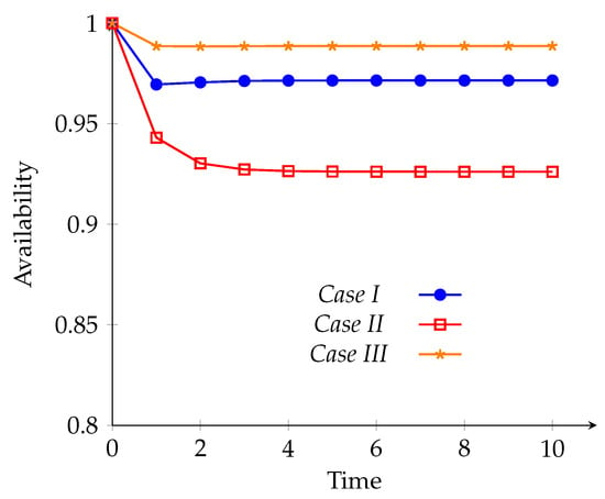
Case I: The following presents an availability analysis using the Gumbel–Hougaard family of copulas; here we set the Gumbel–Hougaard copula parameter to $\psi$ = 1, which corresponds to the independence boundary of this copula family. This choice provides a conservative baseline for comparing the copula-based repair structure with the general independent repair model (Case II), while ensuring mathematical tractability. Even at this boundary, the copula-based formulation remains structurally distinct from the general repair model, as demonstrated in the results below.

Now we calculate the repair rates. Let

$${\stackrel{*}{S}}_{\nu }\left(s\right)={\displaystyle \frac{exp{[x^{\psi }+{\left\{log\sigma \left(x\right)\right\}}^{\psi }]}^{\frac{1}{\psi }}}{s+exp{[x^{\psi }+{\left\{log\sigma \left(x\right)\right\}}^{\psi }]}^{\frac{1}{\psi }}}},{\stackrel{*}{S}}_{\sigma }\left(s\right)={\displaystyle \frac{\sigma }{s+\sigma }},$$

The inverse Laplace transform is then applied to Equation (37), with parameters ${\lambda }_1=0.02,{\lambda }_2=0.03,{\lambda }_3=0.04,{\lambda }_4=0.05,{\lambda }_5=0.06,$ in addition to$\psi =\sigma =x=1$ and $\sigma \left(x\right)=1$. This yields

$$\begin{array}{c}{\stackrel{*}{P}}_{up}\left(t\right)=0.971485+0.0495461e^{-2.86381t}-0.0209364e^{-1.47799t}+0.0000299633e^{-1.16308t}\hfill \\ -0.0000304548e^{-1.13379t}-0.0000390421e^{-1.11286t}-0.0000473008e^{-1.03816t}-8.15711\left({10}^{-6}\right)e^{-1.02443t}\\ +3.13275\left({10}^{-13}\right)e^{-0.21t}-5.53715\left({10}^{-12}\right)e^{-0.16t}-3.53905\left({10}^{-12}\right)e^{-0.14t}-1.73118\left({10}^{-12}\right)e^{-0.12t}\\ \hfill +1.46447\left({10}^{-12}\right)e^{-0.1t}+2.10559\left({10}^{-13}\right)e^{-0.09t}\end{array}$$

(39)

Case II: Availability of system in relation to general repairs.

The use of generalized distributions enables a robust estimation of repair rates in availability analysis.

$${\stackrel{*}{S}}_{\nu }\left(s\right)={\displaystyle \frac{\nu }{s+\nu }},{\stackrel{*}{S}}_{\sigma }\left(s\right)={\displaystyle \frac{\sigma }{s+\sigma }}$$

As seen in Equation (37), the availability is established by assigning specific numerical values to the failure and repair rates.

$$\begin{array}{c}{\stackrel{*}{P}}_{up}\left(t\right)=0.92611+0.0603506e^{-1.60687t}-0.000225423e^{-1.16275t}+0.000323631e^{-1.13421t}\hfill \\ +0.000485524e^{-1.11348t}+0.00336333e^{-1.04105t}+0.00104453e^{-1.02525t}+0.00854873e^{-1.01225t}\\ -1.57567\left({10}^{-12}\right)e^{-0.21t}+6.32974\left({10}^{-12}\right)e^{-0.16t}+2.89056\left({10}^{-12}\right)e^{-0.14t}+6.81107\left({10}^{-12}\right)e^{-0.12t}\\ \hfill +4.62524\left({10}^{-12}\right)e^{-0.1t}+1.07036\left({10}^{-13}\right)e^{-0.09t}\end{array}$$

(40)

In particular, even with $\psi$ = 1 (the independence boundary), Case I (copula-based repair) achieves steady-state availability of 0.971485, which is significantly higher than Case II (general distribution repair) at 0.92611. This indicates that the structural differences in repair rate coupling within the copula framework beyond the mere value of the dependence parameter contribute to improved system performance.

Case III: Reduction approach.

Compared to the initial design, the system’s availability can be improved by introducing a reduction factor $\rho$ ($0<\rho <1$, here $\rho =0.4$) to scale the component failure rates.

$$\begin{array}{c}{\stackrel{*}{P}}_{up}\left(t\right)=0.98862+0.0145337e^{-2.75847t}-0.00313103e^{-1.19177t}+2.34569\left({10}^{-6}\right)e^{-1.0645t}\hfill \\ -7.74301\left({10}^{-6}\right)e^{-1.05325t}-0.0000100015e^{-1.04466t}-6.27705\left({10}^{-6}\right)e^{-1.01539t}-8.97404\left({10}^{-7}\right)e^{-1.00977t}\\ +8.92311\left({10}^{-14}\right)e^{-0.084t}-1.97773\left({10}^{-12}\right)e^{-0.064t}+8.83275\left({10}^{-12}\right)e^{-0.056t}-8.41526\left({10}^{-12}\right)e^{-0.048t}\\ \hfill +1.25307\left({10}^{-12}\right)e^{-0.04t}-1.24698\left({10}^{-12}\right)e^{-0.036t}\end{array}$$

(41)

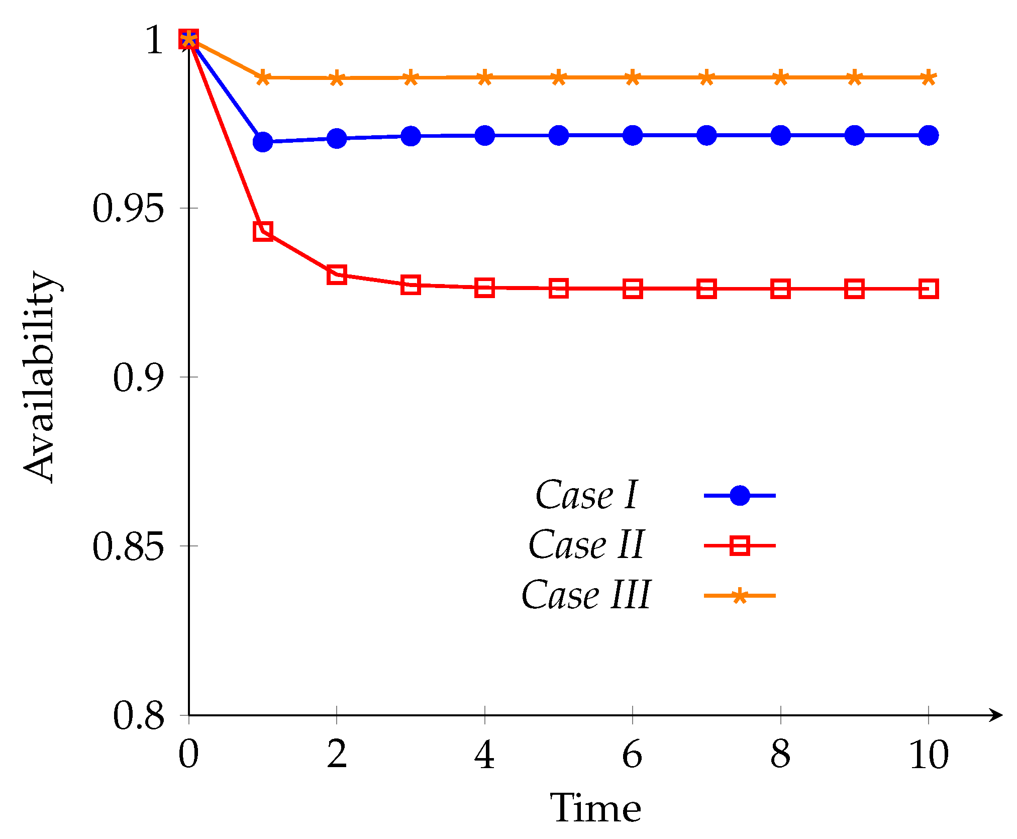
When the time variable t is allowed to range from 0 to 10, the plot shown in Figure 3 and the corresponding data presented in Table 2 are produced by Equations (39)–(41).

Figure 3. System availability over time for Case I (copula-based repair), Case II (general distribution repair), and Case III (reduction approach, $\rho$ = 0.4).

Table 2. System availability under three scenarios (copula-based repair, general distribution repair, and reduction method with $\rho =0.4$) over time t = 0 to 10.

Time	Case I	Case II	Case III
0	1	1	1
1	0.969504	0.943073	0.988583
2	0.970546	0.930283	0.988387
3	0.971242	0.927224	0.988535
4	0.971428	0.926433	0.988593
5	0.971472	0.92621	0.988612
6	0.971482	0.926143	0.988618
7	0.971485	0.926121	0.988619
8	0.971485	0.926114	0.98862
9	0.971485	0.926111	0.98862
10	0.971485	0.92611	0.98862

4.2. System Reliability Analysis and Evaluation

The reliability function is then obtained by applying the inverse Laplace transform to Equation (37), with the repair rates set to zero.

Case I: The failure values presented in Section 4.1 serve as the primary input for assessing system reliability. This approach follows the same methodology used for availability analysis and is grounded in equal probability assumptions. Consequently, this method provides a complementary perspective on system reliability, distinct from traditional failure-rate-based assessments.

$$\begin{array}{c}R\left(t\right)=-0.429411e^{-0.49t}+0.714286e^{-0.21t}+0.0909091e^{-0.16t}+0.342857e^{-0.14t}\hfill \\ \hfill +0.243243e^{-0.12t}+0.0246154e^{-0.1t}+0.0135e^{-0.09t}\end{array}$$

(42)

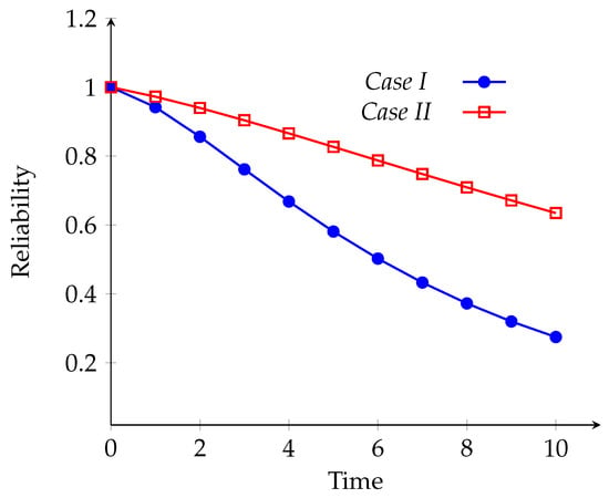
Case II: The reduction strategy decreases the failure rates of system components by a factor of $\rho \in (0,1)$, with $\rho =0.4$, used in this study. This can be demonstrated by substituting the parameter values from Section 4.1 into Equation (37) and evaluating the inverse Laplace transform.

$$\begin{array}{c}R\left(t\right)=-0.351996e^{-0.196t}+0.714286e^{-0.084t}+0.0363636e^{-0.064t}+0.342857e^{-0.056t}\hfill \\ \hfill +0.243243e^{-0.048t}+0.00984615e^{-0.04t}+0.0054e^{-0.036t}\end{array}$$

(43)

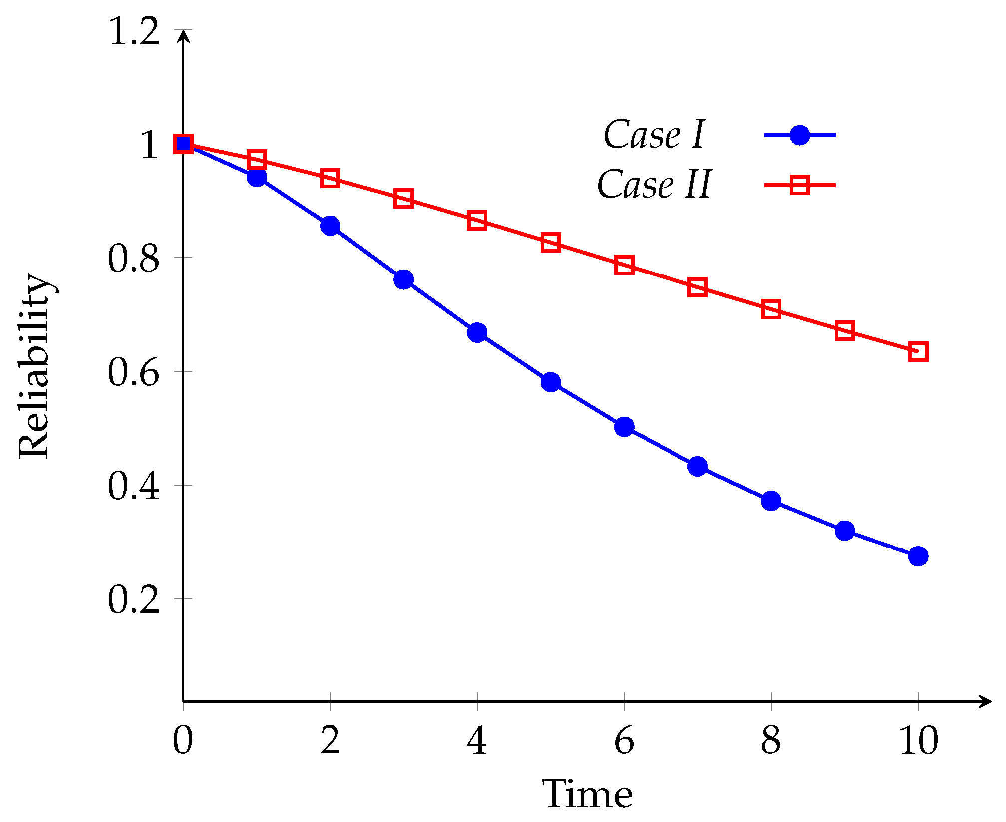
The reliability values R(t), shown in Table 3 and Figure 4, exhibit notable variations when derived using Equations (42) and (43).

Table 3. System reliability R(t) at discrete time intervals (t = 0–10) for Case I (baseline) and Case II ($\rho$ = 0.4).

Time	Case I	Case II
0	1	1
1	0.941802	0.972198
2	0.856067	0.939595
3	0.761463	0.903711
4	0.668091	0.86575
5	0.581039	0.826656
6	0.502508	0.787165
7	0.433089	0.747844
8	0.372515	0.709123
9	0.320098	0.671325
10	0.274981	0.634683

Figure 4. System reliability R(t) over time under Case I (baseline failure rates) and Case II (reduced failure rates, $\rho$ = 0.4).

4.3. Evaluation and Estimation Mean Time to Failure $MTTF$

Taking the limit as s tends to 0 and setting the number of repairs to zero, Equation (37) yields the mean time to failure ($MTTF$).

$$MTTF=\underset{s\to 0}{lim}{\stackrel{*}{P}}_{up}\left(s\right)$$

$$\begin{array}{c}MTTF={\displaystyle \frac{1}{{\lambda }_1+3{\lambda }_2+3{\lambda }_3+4{\lambda }_4+{\lambda }_5}}[1+3{\lambda }_2\left({\displaystyle \frac{2{\lambda }_2}{{\lambda }_2+{\lambda }_5}}+{\displaystyle \frac{1}{2{\lambda }_2+{\lambda }_5}}\right)+3{\lambda }_3\left({\displaystyle \frac{2{\lambda }_3}{{\lambda }_3+{\lambda }_5}}+{\displaystyle \frac{1}{2{\lambda }_3+{\lambda }_5}}\right)\hfill \\ \hfill +4{\lambda }_4\left({\displaystyle \frac{3{\lambda }_4}{2{\lambda }_4+{\lambda }_5}}+{\displaystyle \frac{1}{3{\lambda }_4+{\lambda }_5}}\right)]\end{array}$$

(44)

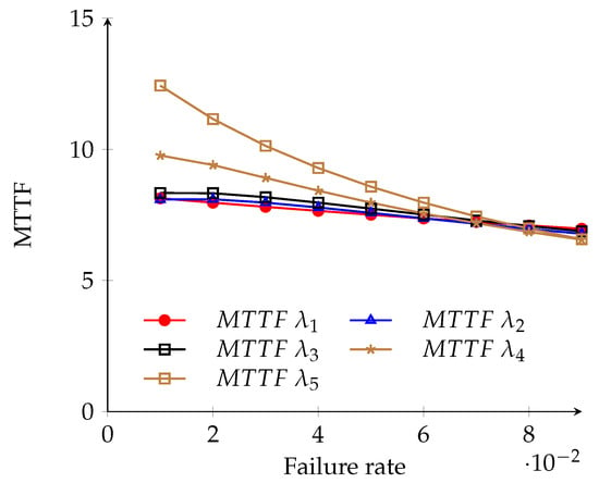
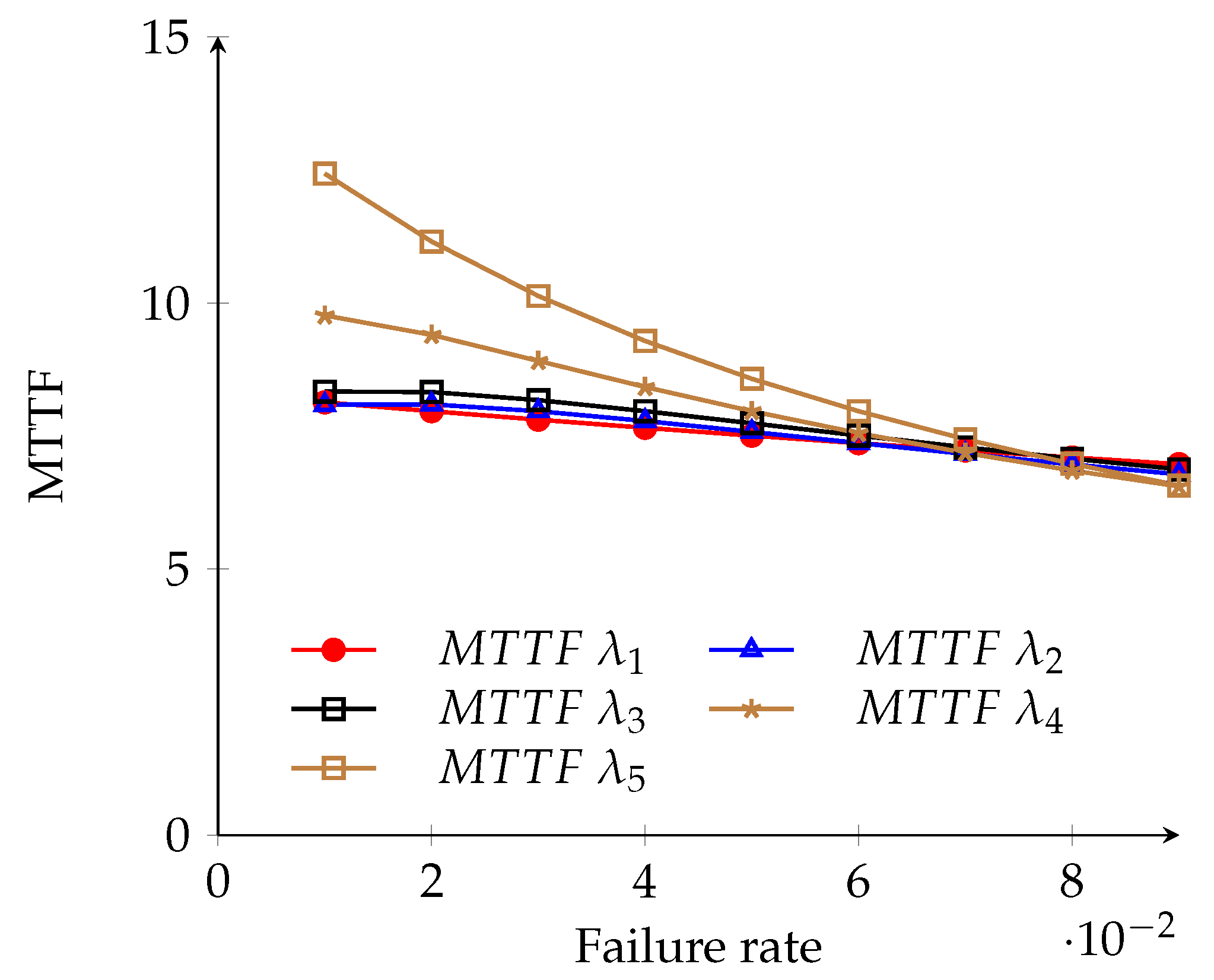
We examine the influence of different parameter values (${\lambda }_1=0.02$, ${\lambda }_2=0.03$, ${\lambda }_3=0.04$, ${\lambda }_4=0.05$, and ${\lambda }_5=0.06$) on the $MTTF$ by individually varying each parameter. Specifically, ${\lambda }_1$, ${\lambda }_2$, ${\lambda }_3$, ${\lambda }_4$, and ${\lambda }_5$ are each varied within the range [0.01, 0.10], as given in Equation (44). Table 4 presents the variations in $MTTF$ corresponding to these changes in failure rates, while Figure 5 illustrates the same.

Table 4. $MTTF$ values are calculated as each failure rate ${\lambda }_1$–${\lambda }_5$ is adjusted individually from 0.01 to 0.09, while other parameters remain constant at baseline.

Failure Rates	MTTF (${\mathit{\lambda }}_1$)	MTTF (${\mathit{\lambda }}_2$)	MTTF (${\mathit{\lambda }}_3$)	MTTF (${\mathit{\lambda }}_4$)	MTTF (${\mathit{\lambda }}_5$)
0.01	8.1313	8.08511	8.33363	9.76542	12.429
0.02	7.96535	8.09353	8.3253	9.39949	11.1544
0.03	7.80605	7.96535	8.17365	8.9101	10.1303
0.04	7.65299	7.78109	7.96535	8.42039	9.28523
0.05	7.50582	7.57616	7.73797	7.96535	8.5738
0.06	7.3642	7.36728	7.50887	7.5531	7.96535
0.07	7.22782	7.16259	7.28627	7.18277	7.43828
0.08	7.09641	6.96597	7.07389	6.85066	6.97682
0.09	6.96969	6.77914	6.87325	6.55239	6.56915

Figure 5. $MTTF$ as a function of the failure rates ${\lambda }_1$ through ${\lambda }_5$, which vary independently and range from 0.01–0.09.

4.4. Sensitivity Study of the Mean Time to Failure $MTTF$

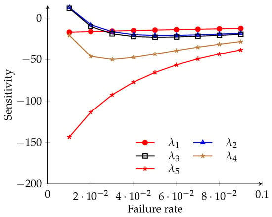
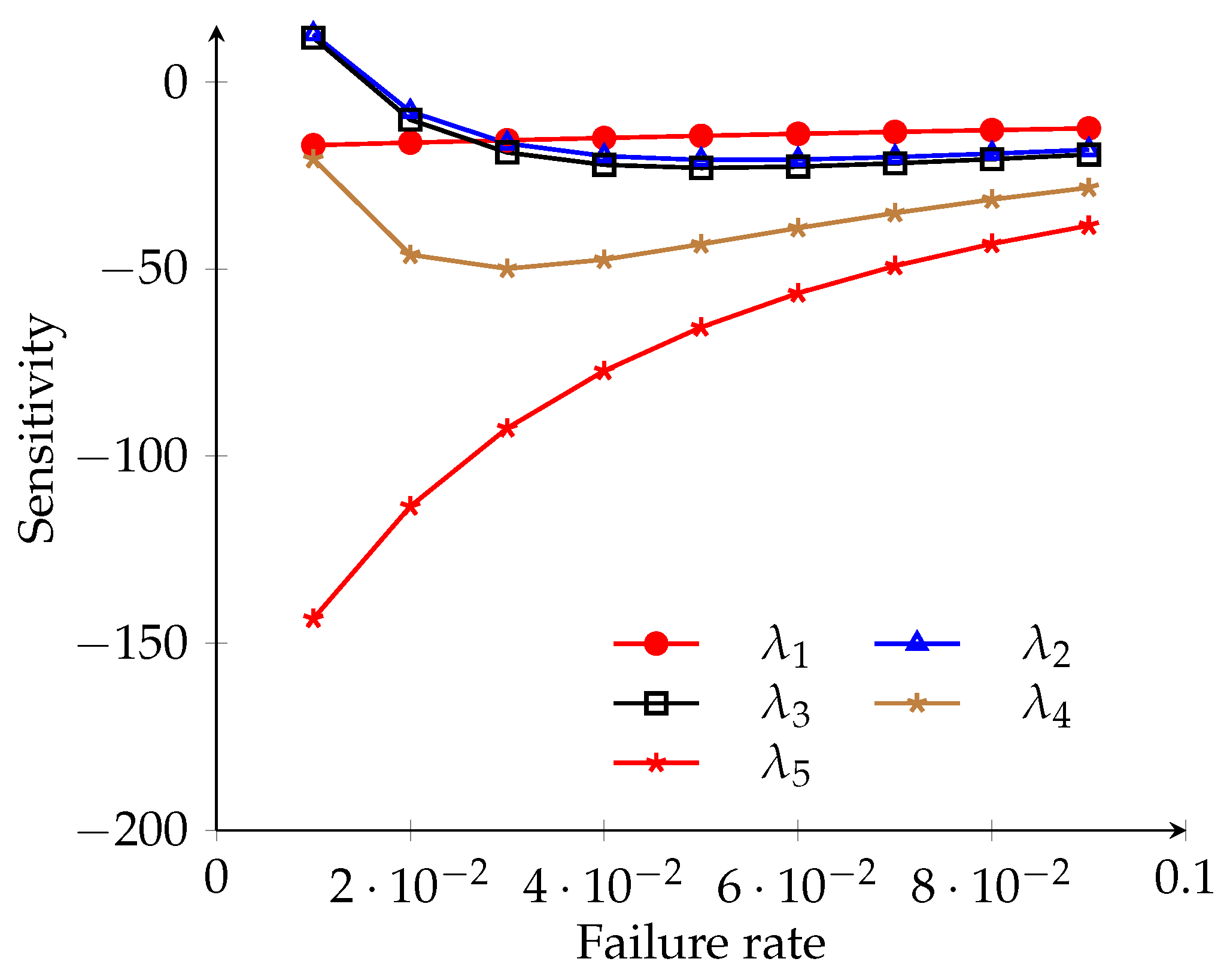
The partial derivatives of the mean time to failure ($MTTF$) with respect to the failure rates provide insight into the sensitivity of the model. By calculating the partial derivatives of Equation (44) and substituting the values ${\lambda }_1=0.04$, ${\lambda }_2=0.05$, ${\lambda }_3=0.06$, ${\lambda }_4=0.07$, and ${\lambda }_5=0.08$, the corresponding sensitivity values are obtained. These values are illustrated in Figure 6 and summarized in Table 5.

Figure 6. The sensitivity of $MTTF$ concerning each failure rate parameter assessed within the interval of 0.01 to 0.09, indicates that the environmental failure rate ${\lambda }_5$ has the most significant adverse effect on system $MTTF$.

Table 5. Sensitivity values calculated at baseline parameter values (${\lambda }_1=0.04$, ${\lambda }_2=0.05$, ${\lambda }_3=0.06$, ${\lambda }_4=0.07$, ${\lambda }_5=0.08$) over the failure rate spectrum of 0.01 to 0.09, measuring the incremental effect of each failure rate on system $MTTF$.

Failure Rates	$\frac{\mathit{\partial }\left(\mathit{M}\mathit{T}\mathit{T}\mathit{F}\right)}{\mathit{\partial }{\mathit{\lambda }}_1}$	$\frac{\mathit{\partial }\left(\mathit{M}\mathit{T}\mathit{T}\mathit{F}\right)}{\mathit{\partial }{\mathit{\lambda }}_2}$	$\frac{\mathit{\partial }\left(\mathit{M}\mathit{T}\mathit{T}\mathit{F}\right)}{\mathit{\partial }{\mathit{\lambda }}_3}$	$\frac{\mathit{\partial }\left(\mathit{M}\mathit{T}\mathit{T}\mathit{F}\right)}{\mathit{\partial }{\mathit{\lambda }}_4}$	$\frac{\mathit{\partial }\left(\mathit{M}\mathit{T}\mathit{T}\mathit{F}\right)}{\mathit{\partial }{\mathit{\lambda }}_5}$
0.01	−16.9402	12.7012	11.7899	−20.6274	−143.45
0.02	−16.2558	−7.94693	−10.1184	−46.1926	−113.438
0.03	−15.6121	−16.4546	−18.8862	−49.936	−92.5346
0.04	−15.0059	−19.8454	−22.1886	−47.5026	−77.2157
0.05	−14.4343	−20.877	−23.015	−43.3939	−65.5722
0.06	−13.8947	−20.7695	−22.6747	−39.08	−56.4724
0.07	−13.3849	−20.108	−21.7878	−35.0507	−49.2015
0.08	−12.9026	−19.189	−20.6635	−31.4463	−43.2858
0.09	−12.4459	−18.1678	−19.4606	−28.278	−38.3994

4.5. Cost Analysis

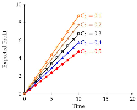
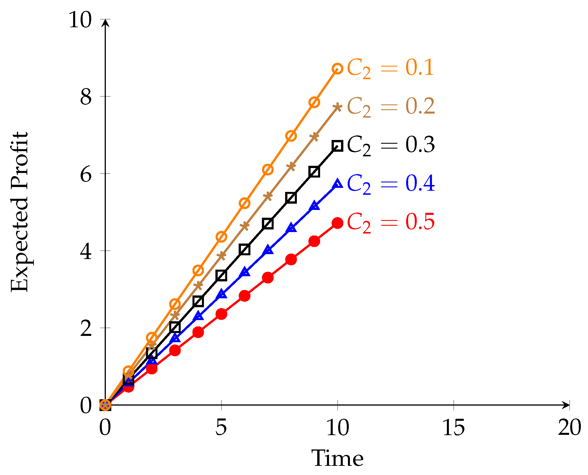
Using the following computational procedure, we can evaluate the system’s expected profit over the interval [0, t], assuming the service facility operates continuously:

$$E_p\left(t\right)=C_1{\int }_0^t{P}_{up}\left(t\right)dt-C_{2}t$$

(45)

Case I: Let $C_1$ represent the revenue generated and $C_2$ denote the service expenditure. We also use the same parameter values as those employed in Equations (37) and (45) from Case I of Section 4.1; the results will be consistent with those obtained in Equation (46). The anticipated profit figures are presented in Table 6, along with a graphical representation in Figure 7.

$$\begin{array}{c}{E}_p\left(t\right)=(0.00304559-0.0173007e^{-2.86381t}+0.0141654e^{-1.47799t}-0.000025762e^{-1.16308t}\hfill \\ +0.000026861e^{-1.13379t}+0.0000350827e^{-1.11286t}+0.000045562e^{-1.03816t}+7.9626\left({10}^{-6}\right)e^{-1.02443t}\\ -1.49178\left({10}^{-12}\right)e^{-0.21t}+3.46072\left({10}^{-11}\right)e^{-0.16t}+2.52789\left({10}^{-11}\right)e^{-0.14t}+1.44265\left({10}^{-11}\right)e^{-0.12t}\\ \hfill -1.46447\left({10}^{-11}\right)e^{-0.1t}-2.33955\left({10}^{-12}\right)e^{-0.09t}+0.971485t)C_1-C_{2}t\end{array}$$

(46)

Table 6. Expected profit $E_p\left(t\right)$ at discrete time intervals (t = 0 to 10) under Case I (copula-based repair) for five service cost levels ($C_2$ = 0.1 to 0.5) with a revenue rate of $C_1$ = 1.

Time	${\mathit{C}}_2=0.5$	${\mathit{C}}_2=0.4$	${\mathit{C}}_2=0.3$	${\mathit{C}}_2=0.2$	${\mathit{C}}_2=0.1$
0	0	0	0	0	0
1	0.476806	0.576806	0.676806	0.776806	0.876806
2	0.946708	1.14671	1.34671	1.54671	1.74671
3	1.41767	1.71767	2.01767	2.31767	2.61767
4	1.88903	2.28903	2.68903	3.08903	3.48903
5	2.36048	2.86048	3.36048	3.86048	4.36048
6	2.83196	3.43196	4.03196	4.63196	5.23196
7	3.30344	4.00344	4.70344	5.40344	6.10344
8	3.77493	4.57493	5.37493	6.17493	6.97493
9	4.24641	5.14641	6.04641	6.94641	7.84641
10	4.7179	5.7179	6.7179	7.7179	8.7179

Figure 7. The expected profit $E_p\left(t\right)$ as a function of time (t = 0 to 20) under Case I (copula-based repair) for five service cost levels ($C_2$ = 0.1, 0.2, 0.3, 0.4, 0.5) with a fixed revenue rate $C_1$ = 1 demonstrates linear profit growth when $C_1>C_2$.

Case II: Cost Analysis Under a General Distribution.

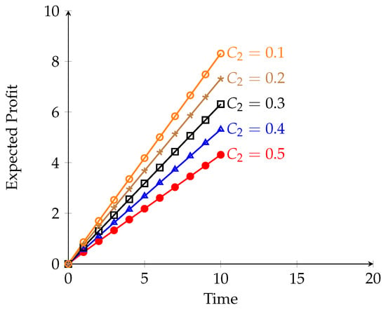
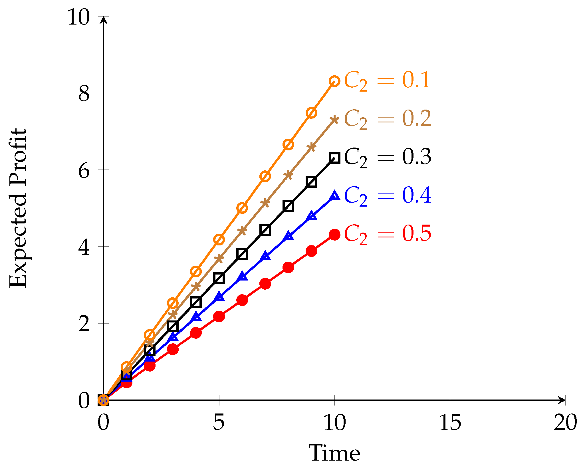
Using the same assumptions stated in Section 4.1, Case II, and applying Equations (37) and (45), Equation (47) is derived. The expected profit results are presented in Table 7, and Figure 8 displays them graphically.

$$\begin{array}{c}{E}_p\left(t\right)=(0.0507803-0.037558e^{-1.60687t}+0.00019387e^{-1.16275t}-0.000285335e^{-1.13421t}\hfill \\ -0.000436042e^{-1.11348t}-0.00323072e^{-1.04105t}-0.00101881e^{-1.02525t}-0.00844531e^{-1.01225t}\\ +7.50321\left({10}^{-12}\right)e^{-0.21t}-3.95609\left({10}^{-11}\right)e^{-0.16t}-2.06468\left({10}^{-11}\right)e^{-0.14t}-5.67589\left({10}^{-11}\right)e^{-0.12t}\\ \hfill -4.62524\left({10}^{-11}\right)e^{-0.1t}-1.18929\left({10}^{-12}\right)e^{-0.09t}+0.92611t)C_1-C_{2}t\end{array}$$

(47)

Table 7. Expected profit $E_p\left(t\right)$ at discrete time intervals (t = 0 to 10) under Case II (general distribution repair) for five service cost levels ($C_2$ = 0.1 to 0.5) with a revenue rate of $C_1$ = 1.

Time	${\mathit{C}}_2=0.5$	${\mathit{C}}_2=0.4$	${\mathit{C}}_2=0.3$	${\mathit{C}}_2=0.2$	${\mathit{C}}_2=0.1$
0	0	0	0	0	0
1	0.464609	0.564609	0.664609	0.764609	0.864609
2	0.899783	1.09978	1.29978	1.49978	1.69978
3	1.32819	1.62819	1.92819	2.22819	2.52819
4	1.75494	2.15494	2.55494	2.95494	3.35494
5	2.18124	2.68124	3.18124	3.68124	4.18124
6	2.60741	3.20741	3.80741	4.40741	5.00741
7	3.03354	3.73354	4.43354	5.13354	5.83354
8	3.45965	4.25965	5.05965	5.85965	6.65965
9	3.88577	4.78577	5.68577	6.58577	7.48577
10	4.31188	5.31188	6.31188	7.31188	8.31188

Figure 8. Expected profit $E_p\left(t\right)$ in Case II (general distribution repair) with service cost levels $C_2$ ranging from 0.1 to 0.5, with $C_1$ set at 1.

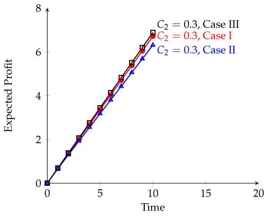
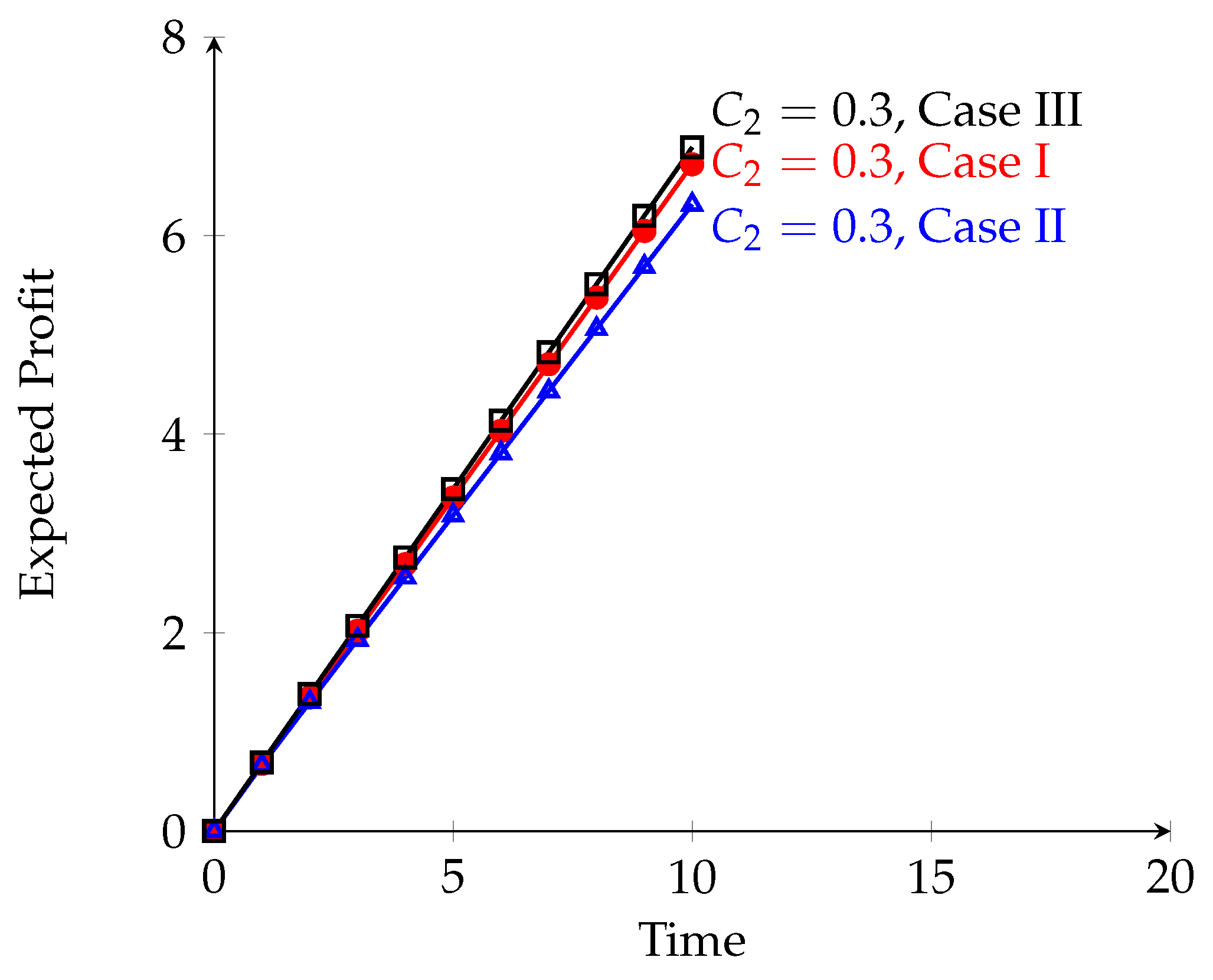
Case III: Analysis of costs using the reduction method.

Applying the same conditions defined in Section 4.1 (Case III) along with Equations (37) and (45), Equation (48) is derived. Table 8 summarizes the expected profit values, while Figure 9 illustrates these results graphically.

$$\begin{array}{c}{E}_p\left(t\right)=(0.00261975-0.00526875e^{-2.75847t}+0.0026272e^{-1.19177t}-2.20356\left({10}^{-6}\right)e^{-1.0645t}\hfill \\ +7.35155\left({10}^{-6}\right)e^{-1.05325t}+9.57391\left({10}^{-6}\right)e^{-1.04466t}+6.1819\left({10}^{-6}\right)e^{-1.01539t}+8.88719\left({10}^{-7}\right)e^{-1.00977t}\\ -1.06227\left({10}^{-12}\right)e^{-0.084t}+3.0902\left({10}^{-11}\right)e^{-0.064t}-1.57728\left({10}^{-10}\right)e^{-0.056t}+1.75318\left({10}^{-10}\right)e^{-0.048t}\\ \hfill -3.13267\left({10}^{-11}\right)e^{-0.04t}+3.46384\left({10}^{-11}\right)e^{-0.036t}+0.98862t)C_1-C_{2}t\end{array}$$

(48)

Table 8. The comparative expected profit $E_p\left(t\right)$ at discrete time intervals (t = 0 to 10) across three scenarios (Case I: copula-based repair; Case II: general distribution repair; Case III: reduction method with $\rho$ = 0.4) at fixed cost parameters $C_2$ = 0.3 and $C_1$ = 1, substantiates Case III as the most economically advantageous configuration.

Time	Origin (${\mathit{C}}_2=0.3$)	General (${\mathit{C}}_2=0.3$)	$\mathit{\rho }=0.4$ (${\mathit{C}}_2=0.3$)
0	0	0	0
1	0.676806	0.664609	0.691711
2	1.34671	1.29978	1.38008
3	2.01767	1.92819	2.06855
4	2.68903	2.55494	2.75712
5	3.36048	3.18124	3.44573
6	4.03196	3.80741	4.13434
7	4.70344	4.43354	4.82296
8	5.37493	5.05965	5.51158
9	6.04641	5.68577	6.2002
10	6.7179	6.31188	6.88882

Figure 9. The comparative expected profit $E_p\left(t\right)$ as a function of time (t = 0 to 20) across three situations at $C_2$ = 0.3 and $C_1$ = 1—namely, Case I (copula-based repair), Case II (general distribution repair), and Case III (reduction method with $\rho$ = 0.4)—demonstrates that the reduction approach produces the largest profit.

The improvement in system performance achieved through the reduction technique is illustrated in Table 8 and Figure 9, for parameter values $C_1=1$; $C_2=0.1$ to $0.5$; during the time interval ranging from 0 to 10.

4.6. Comparison with Existing Reliability Models

• We compare our steady-state availability under copula-based repair (Case I: 0.971485) with the two-subsystem copula repair model of Singh et al. [4], which reports availability values ranging from 0.91 to 0.95 for similar failure rate configurations. The higher steady-state availability of our four-subsystem model is consistent with its more elaborate redundancy structure, incorporating 1-out-of-3 and 2-out-of-4 voting configurations, compared to the 1-out-of-2 configuration in [4].
• Our $MTTF$ results (Table 4) are benchmarked against those reported by Raghav et al. [20], whose two-subsystem copula-repair model reports yields $MTTF$ values of approximately 6.8–7.2 time units under comparable failure rate ranges. Our model produces $MTTF$ values of 7.5–9.8, an improvement attributable to the additional redundancy levels incorporated in Subsystems 2, 3, and 4.
• The sensitivity analysis (Table 5, Figure 6) reveals that the environmental failure rate ${\lambda }_5$ is the primary driver of $MTTF$ degradation, a finding that is qualitatively consistent with Yusuf et al. [21], who similarly report that shared environmental stressors exert the strongest negative influence on system-level availability in communication network models.

5. Conclusions

This study develops and analyzes a mathematical model for a four-subsystem hybrid system motivated by WSN applications in smart agriculture and industrial monitoring. The model captures the reliability characteristics of systems in which multiple redundant components must remain operational to ensure uninterrupted data transmission and monitoring.

5.1. Key Findings

The analysis of three cases yields the following key findings.

Case I (Copula-Based Repair):

• The steady-state availability is 0.971485 (at $\psi$ = 1); see Table 2.
• This case demonstrates superior performance over general distribution repair (Case II), even at the independence boundary of the copula, owing to the structurally coupled repair formulation.
• The expected profit increases linearly over time when $C_1$ exceeds $C_2$ (Figure 7).

Case II (General Distribution Repair):

• Steady-state availability: 0.92611 (see Table 2).
• This value is inferior to that of the copula-based approach, underscoring the importance of modeling repair time dependencies.
• The expected profit is lower than that of Case I under equivalent cost parameters (see Table 7).

Case III (Reduction Method with $\rho =0.4$):

• Steady-state availability: 0.98862 (see Table 2).
• Achieved by multiplying the failure rates by a reduction factor of $\rho =0.4$.
• Represents a 1.8% improvement over Case I and a 6.8% improvement over Case II.
• Yields the maximum expected profit across all considered cases (Table 8, Figure 9).

5.2. Practical Implications for WSN Design

For WSN system designers and operators, our findings offer several actionable insights.

• Repair Strategy: Implementing coordinated multi-unit repair, where inter-unit dependency is modeled via a copula function, improves system availability by 5% over independent repair strategies (Cases I vs. II).
• Component Quality Investment: The failure-rate reduction technique (Case III) demonstrates that investing in higher-quality components ($\rho$ = 0.4) yields notable reliability improvements, thereby justifying the potentially higher procurement costs.
• Sensitivity Analysis: Table 5 and Figure 6 reveal that the environmental failure rate (${\lambda }_5$) exerts the strongest negative influence on $MTTF$, suggesting that protective enclosures and environmental hardening measures offer the highest return on investment.
• Economic Viability: Cost analysis (Table 6, Table 7 and Table 8) demonstrates that system profitability is highly sensitive to service costs ($C_2$), with the break-even point occurring as ($C_2$) converges toward the revenue rate ($C_1$).

5.3. Limitations and Future Work

This study is subject to several limitations that warrant acknowledgment and suggest directions for future investigation.

• The model assumes perfect repair (i.e., as-good-as-new restoration), an assumption that may not be valid for aging WSN components.
• The environmental failure rate (${\lambda }_5$) is treated as constant, whereas practical deployments are subject to seasonal and diurnal variations.
• The reduction method assumes a uniform decrease in failure rates across all components; the potential benefits of heterogeneous improvement strategies remain unexplored.

Future research should incorporate the following:

• Imperfect repair models and component degradation.
• Time-varying failure rates reflecting environmental conditions.
• Multi-objective optimization balancing cost, reliability, and energy consumption.
• Experimental validation using real WSN deployment data.

References

- Catelani, M.; Ciani, L.; Bartolini, A.; Del Rio, C.; Guidi, G.; Patrizi, G. Reliability Analysis of Wireless Sensor Network for Smart Farming Applications. Sensors 2021, 21, 7683. [Google Scholar] [CrossRef] [Scilit] [PubMed]
- Jesus, T.C.; Portugal, P.; Vasques, F.; Costa, D.G. Automated methodology for dependability evaluation of wireless visual sensor networks. Sensors 2018, 18, 2629. [Google Scholar] [CrossRef] [Scilit] [PubMed]
- Lechang, Y.; Jinwei, W.; Min, X. Graph-based reliability evaluation of a reconfigurable multi-stage system using sequential unconnected path sets. Reliab. Eng. Syst. Saf. 2025, 261, 111093. [Google Scholar] [CrossRef] [Scilit]
- Singh, V.V.; Lado, A.K. Cost assessment of complex repairable system consisting two subsystems in Series configuration using Gumbel–Hougaard family copula. Int. J. Qual. Reliab. Manag. 2019, 36, 1683–1698. [Google Scholar]
- Elshoubary, E.E.; Radwan, T. Studying the Efficiency of the Apache Kafka System Using the Reduction Method, and Its Effectiveness in Terms of Reliability Metrics Subject to a Copula Approach. Appl. Sci. 2024, 14, 6758. [Google Scholar] [CrossRef] [Scilit]
- Elshoubary, E.E.; Radwan, T.; Attwa, R.A.E.-W. Reliability and Performance Optimization of Multi-Subsystem Systems Using Copula-Based Repair. Axioms 2025, 14, 163. [Google Scholar] [CrossRef] [Scilit]
- Sohraby, K.; Minoli, D.; Znati, T. Wireless Sensor Networks—Technology, Protocols and Applications; John Wiley & Sons, Inc.: Hoboken, NJ, USA, 2007. [Google Scholar]
- Oszczypała, M.; Konwerski, J.; ZiOlkowski, J.; Małachowski, J. Reliability analysis and redundancy optimization of k-out-of-n systems with random variable k using Continuous Time Markov Chain and Monte Carlo simulation. Reliab. Eng. Syst. Saf. 2024, 242, 109780. [Google Scholar] [CrossRef] [Scilit]
- Ogura, N.; Kasuya, M.; Jin, L. Joint Optimal Policy for Maintenance, Spare Unit Selection and Inventory Control Under a Partially Observable Markov Decision Process. Mathematics 2025, 13, 406. [Google Scholar] [CrossRef] [Scilit]
- Kumar, A.; Jadhav, S.; Alsalami, O. Reliability and Sensitivity Analysis of Wireless Sensor Network Using a Continuous-Time Markov Process. Mathematics 2024, 12, 3057. [Google Scholar] [CrossRef] [Scilit]
- Zhao, J.; Liang, M.; Tian, R.; Zhang, Z.; Cao, X. Reliability Optimization of Hybrid Systems Driven by Constraint Importance Measure Considering Different Cost Functions. Mathematics 2023, 11, 4283. [Google Scholar] [CrossRef] [Scilit]
- Addabbo, T.; Fort, A.; Landi, E.; Mugnaini, M.; Panzardi, E.; Pozzebon, A.; Vignoli, V. Reliability and Availability Evaluation of Linear LoRaWAN Sensor Network Architectures for Pipeline Monitoring. In Proceedings of the 2020 IEEE International Instrumentation and Measurement Technology Conference (I2 MTC), Dubrovnik, Croatia, 25–28 May 2020; pp. 1–6. [Google Scholar]
- Denson, W. The history of reliability prediction. IEEE Trans. Reliab. 1998, 47, SP321–SP328. [Google Scholar] [CrossRef] [Scilit]
- Catelani, M.; Ciani, L.; Guidi, G.; Galar, D. A Practical Solution for HVAC Life Estimation Using Failure Models. In Proceedings of the 17th IMEKO TC 10 and EUROLAB Virtual Conference, Virtual, 20–22 October 2020; pp. 85–91. Available online: https://hdl.handle.net/11556/8732 (accessed on 16 April 2026).
- IEC 61078; Reliability Block Diagram. International Electrotechnical Commission: Geneva, Switzerland, 2016.
- IEC 61025; Fault Tree Analysis (FTA). International Electrotechnical Commission: Geneva, Switzerland, 2018.
- Ciani, L.; Guidi, G.; Galar, D. Reliability evaluation of an HVAC ventilation system with FTA and RBD analysis. In Proceedings of the 6th IEEE International Symposium on Systems Engineering, Vienna, Austria, 12 October–12 November 2020; p. 12. [Google Scholar]
- Ciani, L.; Bartolini, A.; Guidi, G.; Patrizi, G. Condition Monitoring of Wind Farm based on Wireless Mesh Network. In Proceedings of the 16th IMEKO TC10 Conference: Testing, Diagnostics & Inspection as a Comprehensive Value Chain for Quality & Safety 2019; International Measurement Federation (IMEKO): Berlin, Germany, 2019; pp. 39–44. [Google Scholar]
- Gokdere, G.; Keung, H. Time-Dependent Reliability Analysis for Repairable Consecutive k-Out-of-n: F System; Statistical Theory, and Related Fields; Taylor& Francis: Abingdon, UK, 2021. [Google Scholar] [CrossRef] [Scilit]
- Raghav, D.; Poonia, P.K.; Gahlot, M.; Singh, V.V.; Hamisu, I.; Ameer, H. Probabilistic analysis of a system consisting of two subsystems in the series configuration under copula repair approach. J. Korean Math. Educ. Soc. Ser. B Pure Appl. Math. 2020, 27, 135–155. [Google Scholar]
- Yusuf, I.; Ismail, A.K.L.; Ali, U.A. Reliability analysis of communication network system with redundant relay station under partial and complete failure. J. Math. Comput. Sci. 2020, 10, 863–880. [Google Scholar] [CrossRef] [Scilit]
- Taghi, S.; Niaki, A.; Yaghoubi, A. Exact equations for the reliability and mean time to failure of 1-out-of-N cold standby system with imperfect switching. J. Optim. Indus. Eng. 2021, 14, 197–203. [Google Scholar]
Disclaimer/Publisher’s Note: The statements, opinions and data contained in all publications are solely those of the individual author(s) and contributor(s) and not of MDPI and/or the editor(s). MDPI and/or the editor(s) disclaim responsibility for any injury to people or property resulting from any ideas, methods, instructions or products referred to in the content. |
© 2026 by the authors. Licensee MDPI, Basel, Switzerland. This article is an open access article distributed under the terms and conditions of the Creative Commons Attribution (CC BY) license.