Article

On the Exploration and Exploitation Capabilities of the Artificial Bee Colony Algorithm

1
Faculty of Electrical Engineering and Computer Science, University of Maribor, Koroška Cesta 46, 2000 Maribor, Slovenia
2
Department of Applied Mathematics, Florida Polytechnic University, 4700 Research Way, Lakeland, FL 33805, USA
*
Author to whom correspondence should be addressed.
Mathematics 2026, 14(9), 1406; https://doi.org/10.3390/math14091406
Submission received: 14 March 2026 / Revised: 16 April 2026 / Accepted: 17 April 2026 / Published: 22 April 2026
(This article belongs to the Section E1: Mathematics and Computer Science)

Abstract

In this paper, we investigate the exploration and exploitation capabilities of the Artificial Bee Colony (ABC) algorithm using novel attraction basin-based measures. Previous claims about the ABC’s weak exploitation and exploration capabilities have been scrutinized. These claims are not based on exploration and exploitation measurements and, as such, are questionable. Direct measurements are needed to get real insights into the exploration and exploitation capabilities of any search algorithm. The results show that indirect measurements based on diversity are not appropriate. Our newly developed attraction basin-based measurements allow us to differentiate between exploration types (successful, failed, deceptive, successful rejection) and exploitation types (successful, unsuccessful). Namely, it is not only important that an algorithm is in the exploration phase, but also that promising regions with better solutions are not abandoned and that regions with worse solutions are visited less frequently. Similarly, during the exploitation phase, it is important to discover better solutions in the neighborhood and not exploit in an unsuccessful direction. It has been shown that ABC’s exploration and exploitation capabilities are versatile, and can adapt to different fitness landscapes successfully.

1. Introduction

The Artificial Bee Colony (ABC) algorithm [1,2] is an interesting metaheuristic algorithm [3,4] inspired by honey bees’ foraging behavior, with three distinct phases: employed bee, onlooker bee, and scout bee. ABC has been applied to numerous real-world optimization problems, such as structural damage detection [5], searching for soil models’ parameters [6], determination of a hysteresis model’s parameters [7], mobile robot path planning [8], determination of DC motor and drive parameters [9], sales forecasting [10], and flow-shop scheduling [11]. ABC has been compared with other metaheuristic algorithms [12], and many variants of ABC exist [13]. Despite ABC’s simple structure and implementation, many researchers have misunderstood how many new solutions are generated in the scout bee phase and how to count the fitness evaluations consumed in that phase correctly. These issues have been reported and discussed in [14]. However, there is yet another widespread misunderstanding about how ABC explores and exploits the search space. The search process is in the exploration phase when new solutions are generated in the previously unvisited search space. Conversely, it is in the exploitation phase when new solutions are generated in the neighborhood of previously visited solutions [15]. It has been widely acknowledged that exploration and exploitation are fundamental and crucial processes of any search algorithm [16], and that the effectiveness of evolutionary algorithms (EAs) can be attributed to the good balance achieved between exploration and exploitation in EAs [17]. In many reports [18,19,20,21,22,23,24,25,26], the authors claim that ABC’s exploration capability is much better than its exploitation capability, despite the fact that the employed bee and onlooker bee phases use the same equation and should generate a new solution in the vicinity of the previous solution, whilst generating a random solution in the scout bee phase. As such, ABC seems to exploit the search space during the employed bee and onlooker bee phases, and to explore it during the scout bee phase [11]. However, without measuring exploration and exploitation directly, these are only assumptions. It is also interesting that the authors in [25] classified the search type for the employed bee and the onlooker bee phases differently, despite the same search equation (Equation (1)) appearing in both phases.
x i j = x i j + ϕ i j ( x i j x k j )
The authors in [25] wrote: “As for the employed bees, they are responsible for searching new food sources in the entire search space, and they can be considered to play the role of exploration. … To some extent, the onlooker bees play the role of exploitation.” The reasoning for the equation used in the employed bee and onlooker bee phases was as follows in [18]: “On the other hand, in Equation (1), the coefficient ϕ i j is a uniform random number in [ 1 , 1 ] and x k j is a random individual in the population, therefore, the solution search dominated by Equation (1) is random enough for exploration. To sum up, the solution search equation described by Equation (1) is good at exploration but poor at exploitation.” Since measuring exploration and exploitation capabilities directly has not been realized up to now, such claims are mere speculations.
The authors in [27] found out that the scout bee phase is activated rarely for high-dimensional problems when standard control parameter settings are used ( l i m i t = S N 2 D ; S N is the population size and D is the dimension of a problem). Since dimension D is high, the control parameter limit is high as well. In the scout bee phase, a new solution is only randomly generated for a previous solution, which has a highest number of unsuccessful attempts on improvements that is equal to or greater than the control parameter limit. The authors in [27] found that in many cases, the best-so-far solutions have the highest number of unsuccessful attempts. Hence, the best-so-far solutions are abandoned in favor of random solutions. In our opinion, this is the main reason for the slow convergence of ABC, not low exploitation capability as claimed by many others [18,19,20,21,22,23,24,25,26]. The authors in [27] also questioned the claim of the good exploration capability of ABC [18,19,20,21,22,23,24,25,26] since the scout bee phase, which is responsible for exploration, is often not activated at all in high-dimensional problems due to the high value of the control parameter limit (when the standard setting is used for control parameter limit). According to [27], the exploration capability of ABC is also weak. Firstly, study [28] shows that the standard control parameter setting for the limit is not conclusively the best setting and should not be used in every scenario (e.g., for high-dimensional problems). Secondly, as the current study shows, exploration in ABC not only happens in the scout bee phase, but also in the employed bee and onlooker bee phases. This has been verified by measuring exploration and exploitation directly using attraction basin-based measures (see Section 3).
On the other hand, the authors in [20] used a slightly different description of exploration and exploitation by writing: “The exploration refers to the ability to investigate the various unknown regions in the solution space to discover the global optimum. While the exploitation refers to the ability to apply the knowledge of previous solutions to find better solutions”, and claiming that ABC is poor in exploitation due to slow convergence (not finding better solutions). Similar definitions of exploration and exploitation also appear in [29]: “Exploration involves searching for new regions of the solution space to avoid local optima, while exploitation refines existing solutions to achieve better convergence.” A fast convergence rate was also used as a measure for exploitation in [21]. The same reasoning was also applied in [23], where the authors measured the number of better solutions obtained and used this as an indicator of ABC’s exploitation ability. However, we should distinguish between exploiting the search space and finding a better solution, and similarly, exploring the search space and finding a better region. The algorithm might be in the process of exploitation, but finding a better solution cannot be guaranteed. Similarly, we cannot claim that an algorithm is not performing exploration if the global optimum is not found. This actually happens in the Random Search Algorithm (RSA), where a global optimum is found rarely, despite RSA’s main search mode being exploration. We need to differentiate between how an algorithm performs the search (exploration and exploitation) and whether an improvement is achieved by finding a better solution or a better region. By our novel direct measure of exploration and exploitation based on attraction basins [30], this can indeed be achieved by differentiating further between exploration types (successful exploration, successful rejection, failed exploration, and deceptive exploration) and exploitation types (successful exploitation, unsuccessful exploitation). The exploitation measure used in [23] actually only measured successful exploitation.
The main contributions of this paper are:
  • A direct measurement of exploration (successful, failed, deceptive, successful rejection) and exploitation (successful, unsuccessful) in the ABC algorithm.
  • An analysis of the influence of ABC’s control parameters on exploration and exploitation.
  • A demonstration and explanation of the limitations of indirect diversity measures for assessing exploration and exploitation using a specially designed EA.
Note that ABC was developed primarily for continuous optimization problems, and only later have ABC’s equations been adjusted for discrete optimization problems [31,32,33]. In this work, we focus solely on measuring ABC’s exploration and exploitation capabilities in continuous optimization problems, while discrete problems are out of scope.
The remainder of this paper is organized as follows: Related work is described in Section 2. The novel approach to measuring exploration and exploitation directly is outlined in Section 3. The experimental results and analysis are presented in Section 4. Finally, Section 5 provides the conclusions of the study and future work.

2. Related Work

Before controlling exploration and exploitation in EAs we need to know how to measure both processes. Unfortunately, this is an open problem in EAs, and researchers primarily use indirect measures, such as diversity- and entropy-based metrics. All these approaches measure exploration and exploitation indirectly under different assumptions. For example, if the diversity of the population is low (high), then exploitation (exploration) is declared [34], or similarly, when the entropy is low (high), then exploitation (exploration) is declared. The most popular diversity-based measure is the dimension-wise diversity measure [35,36,37,38,39], computing the amount of exploration (XPL%) and exploitation (XPT%) as follows [40] (n is the population size, and D is the dimension of a problem):
XPL % = Div Div max × 100
XPT % = | Div Div max | Div max × 100
where
Div j = 1 n i = 1 n mean ( x j ) x i j
Div = 1 D j = 1 D Div j
However, these measures are very coarse and imprecise [30] and can be applied only at the population level. They cannot determine whether a particular new solution is generated in the exploration or exploitation zone.
On the other hand, useful direct measures are difficult to develop, since a neighborhood is difficult to define. In early attempts, a neighborhood is modeled as a hypercube with a user-defined diameter [24,41], or by a hypersphere with a user-defined radius [42]. Clearly, a user-defined diameter/radius is hard to define properly, because it depends on the fitness landscape. Even within the same search space, the ruggedness of the fitness landscape can change drastically [43], and the diameter/radius needs to be adjusted properly. Again, such direct measures, where a neighborhood is modeled by a hypercube or a hypersphere, are not precise enough, but can at least be applied at the individual level, not only at the population level. The authors in [44] suggested that attraction basins might be useful for measuring exploration and exploitation. Based on this recommendation, we proposed in [30] a direct measure for exploration and exploitation using attraction basins with the assumption that a neighborhood consists of all the solutions, which can be simply reached by a local search (e.g., gradient search). Therefore, the user-defined diameter/radius is no longer needed. If the parent and the new solution are in the same (different) attraction basin, then this is identified as exploitation (exploration). Although the idea is interesting, it is impractical, since attraction basins are very expensive to compute. As such, the approach in [30] can be used only for offline analysis. In our subsequent work, we improve the approach so that attraction basins no longer need to be computed, but it is still possible to identify if a parent and a new solution belong to the same (different) attraction basins. Every attraction basin [45] contains a point called the attractor, which corresponds to the basin’s local optimum and can be reached from any point in the attraction basin by a local search. To identify if a parent and a new solution belong to the same (different) attraction basin, we have to compute the parent’s attractor, as well as the new solution’s attractor. If they are the same (different), then we can declare the exploitation (exploration) phase. This approach is much less computationally expensive than computing attraction basins in advance, and is comparable to the computational costs of Memetic Algorithms [46,47]. When greedy survival selection is used, the four different types of exploration (the parent and a new solution are in different attraction basins) can be defined as [48]:
  • Successful exploration (SE): The fitness of a new solution is better than the parent’s fitness, greedy survival selection will preserve a new solution, and the new solution is in a better attraction basin than the parent’s attraction basin. We find a better solution in a better attraction basin, and we can declare the exploration as successful.
  • Successful rejection (SR): The fitness of a new solution is worse than the parent’s fitness, greedy survival selection will preserve the parent, and the new solution is in a worse attraction basin than the parent’s attraction basin. We find a worse solution in a worse attraction basin, and we reject it successfully.
  • Failed exploration (FE): The fitness of a new solution is worse than the parent’s fitness, greedy survival selection will preserve the parent, and the new solution is in a better attraction basin than the parent’s attraction basin. We find a solution in a better attraction basin, but we fail to accept it.
  • Deceptive exploration (DE): The fitness of a new solution is better than the parent’s fitness, greedy survival selection will preserve the new solution, and the new solution is in a worse attraction basin than the parent’s attraction basin. We find a better solution in a worse attraction basin and accept it, moving from an attraction basin with a better local optimum to one with a worse local optimum. This action is undesirable and should be avoided by the search algorithm.
In [48], these four different types of exploration were defined using only the Rastrigin function, since the attraction basins were obtained analytically. Our work demonstrates how the proposed direct measures for exploration and exploitation can be used to analyze the behavior of the ABC algorithm across different optimization problems, and investigates the effects of the control parameter settings. Such an analysis, based on direct exploration and exploitation measures, has not been conducted before. It is fundamentally different from the analysis in [40], which was based on imprecise diversity-based measures of exploration and exploitation, and found that most EAs produced the best results when the balance between exploitation and exploration was approximately 90% to 10%, respectively.
In the literature, we observe many works proposing new approaches intended to improve the balance between exploration and exploitation. However, since exploration and exploitation have not been measured directly, the effect of new proposals is unknown. For example, the authors in [26] proposed a new variant of ABC, called BDLDABC, where new search equations were designed in a manner to promote exploration; coexisting exploration–exploitation; and exploitation for employed bees, onlooker bees, and scout bees, respectively. Although the amount of exploration and exploitation was not measured, it is interesting that the authors acknowledged that, in the proposed onlooker bee phase, both exploration and exploitation could happen.

3. Material and Methods

To analyze exploration in a landscape-aware manner, we propose an attraction basin-based classification of offspring solutions. The approach builds on the concept of attraction basins induced by local search, and aims to quantify both the extent and the outcome of the exploration performed by an algorithm. An attraction basin A ( x * ) is defined as a subset of the search space S associated with a local optimum x * , referred to as the attractor, such that any solution y A ( x * ) converges to x * when a local search procedure is applied [45,49,50,51,52]. Formally, for a deterministic local search operator L ( · ) , all solutions in A ( x * ) satisfy L ( y ) = x * .
Let f ( x ) denote the objective function to be minimized, and consider a population of n parent–offspring pairs ( p i , x i ) in a given generation. In the strict sense, exploration is assumed to occur only when an offspring reaches a different attraction basin than its parent. This is captured by the basin-transition indicator:
δ i = 1 , if L ( x i ) L ( p i ) , 0 , otherwise ,
where δ i = 1 indicates that x i A ( x k * ) and p i A ( x l * ) with x k * x l * . Only such cases are considered genuine exploration events. For each basin transition, the exploration outcome is determined based on the relative quality of the offspring and the parent before and after the local search. A transition is classified as successful exploration if the offspring improves upon its parent both prior to and after local optimization, corresponding to a move to a strictly better attraction basin:
I i S E = 1 , δ i = 1 f ( x i ) < f ( p i ) f ( L ( x i ) ) < f ( L ( p i ) ) , 0 , otherwise .
Deceptive exploration occurs when an offspring is superior before the local search, but converges to a worse attractor, reflecting misleading information in the global search space:
I i D E = 1 , δ i = 1 f ( x i ) < f ( p i ) f ( L ( x i ) ) > f ( L ( p i ) ) , 0 , otherwise ,
In contrast, failed exploration refers to cases where an initially inferior offspring converges to a superior attractor after local optimization:
I i F E = 1 , δ i = 1 f ( x i ) > f ( p i ) f ( L ( x i ) ) < f ( L ( p i ) ) , 0 , otherwise .
Finally, if the offspring is inferior both before and after the local search, the transition is categorized as a successful rejection:
I i S R = 1 , δ i = 1 f ( x i ) > f ( p i ) f ( L ( x i ) ) > f ( L ( p i ) ) , 0 , otherwise .
The relative frequencies of the different exploration outcomes are defined as
S E = 1 E i = 1 n I i S E , D E = 1 E i = 1 n I i D E ,
F E = 1 E i = 1 n I i F E , S R = 1 E i = 1 n I i S R ,
where
E = i = 1 n δ i
denotes the total number of basin transitions observed in the population. By construction, these quantities satisfy S E + D E + F E + S R = 1 .
Unlike traditional diversity measures based solely on spatial dispersion, this metric captures movement directly across the attraction basins, and therefore provides a landscape-aware characterization of the exploration. It is evident that a multimodal search space can be decomposed into multiple attraction basins, each associated with a local optimum, whereas a unimodal search space consists of a single attraction basin containing the global optimum. Illustrations of attraction basins can be found in [30,53]. In the context of evolutionary search, transitions between different attraction basins correspond to exploration, while movements within the same basin represent exploitation. As discussed in the previous section, successful exploration and successful rejection are considered desired exploration ( D E x p l ) outcomes, whereas deceptive and failed exploration are considered undesired exploration ( U E x p l ). A well-performing evolutionary algorithm is therefore expected to exhibit a higher proportion of desired exploration. While [48] focused exclusively on different exploration types, in this work we additionally distinguish between two types of exploitation, defined for parent–offspring pairs that remain within the same attraction basin.
An offspring is considered to be generated through exploitation if it converges to the same attractor as its parent under a local search. Formally, exploitation events are identified using the basin-preservation indicator:
γ i = 1 , if L ( x i ) = L ( p i ) , 0 , otherwise ,
where γ i = 1 indicates that both solutions belong to the same attraction basin.
For each exploitation event, two outcomes are distinguished based on the fitness relation between the offspring and the parent. Successful exploitation ( S E x p t ) occurs when the offspring improves upon its parent while remaining within the same basin, representing a desirable local refinement:
I i S E x p t = 1 , γ i = 1 f ( x i ) < f ( p i ) , 0 , otherwise .
In contrast, unsuccessful exploitation ( U E x p t ) corresponds to cases where the offspring does not improve upon the parent, resulting in no progress despite consuming fitness evaluations:
I i U E x p t = 1 , γ i = 1 f ( x i ) f ( p i ) , 0 , otherwise .
Let
X = i = 1 n γ i
denote the total number of exploitation events in the population. The relative frequencies of successful and unsuccessful exploitation are then given by
S E x p t = 1 X i = 1 n I i S E x p t ,
U E x p t = 1 X i = 1 n I i U E x p t ,
with S E x p t + U E x p t = 1 . These measures quantify the effectiveness of local refinement within attraction basins, complementing the basin-based exploration analysis presented earlier.
In contrast to the previously introduced diversity-based measures XPL% and XPT%, which quantify exploration and exploitation in terms of population diversity, the measures XPL and XPT proposed here capture basin-based exploration and exploitation derived from local search behavior. Since each parent–offspring pair either results in a transition to a different attraction basin or remains within the same basin, exploration and exploitation form a complete partition of the population. Consequently,
XPL = E n , XPT = X n ,
and therefore
XPL + XPT = 1 .
In this work, we apply a direct attraction basin-based measure for exploration and exploitation using the ABC algorithm [1,2]. From the pseudocode of the ABC (Algorithm 1), three distinct phases can be observed: employed bee, onlooker bee, and scout bee. The ABC has a few control parameters: maximum fitness evaluations (MFEs) (in some implementations, a maximum number of cycles—MNC), population size (SN), and maximum number of trials for abandoning a solution (limit). The complexity of ABC and its variants has been discussed in [54]. The main goal of this paper is to measure ABC’s exploration and exploitation capabilities and determine the influence of control parameters on these behaviors.
Algorithm 1 Pseudocode for Artificial Bee Colony (ABC)
Input:  S N : number of food sources (population size)
Input:  l i m i t : maximum number of trials before abandonment
Input:  M F E : maximum number of fitness evaluations
Output:  b e s t S o l u t i o n
Initialize n u m _ e v a l 0
for  s = 1 to S N  do
       X ( s ) generate random solution (Equation (1)) [2]
       f s f ( X ( s ) )
      t r i a l ( s ) 0
      n u m _ e v a l n u m _ e v a l + 1
end for
while  n u m _ e v a l < M F E   do
     for  s 1 to S N  do                                                                ▹ Employed Bees Phase
            x generate new solution by Equation (2) [2]
            f x f ( x )
           n u m _ e v a l n u m _ e v a l + 1
          if  f x < f s  then
                  X ( s ) x
                  f s f x
                  t r i a l ( s ) 0
          else
                  t r i a l ( s ) t r i a l ( s ) + 1
          end if
          if  n u m _ e v a l = M F E  then
                 break
          end if
    end for
    Update b e s t S o l u t i o n
    Compute selection probabilities p i using fitness values (Equations (3) and (4)) [2]
     s 1 , t 1
    while  t < S N and n u m _ e v a l < M F E  do                                           ▹ Onlooker Bees Phase
           r r a n d ( 0 , 1 )
          if  r < p ( s )  then
              t t + 1
              x generate new solution by Equation (2) [2]
              f x f ( x )
              n u m _ e v a l n u m _ e v a l + 1
             if  f x < f s  then
                   X ( s ) x
                   f s f x
                   t r i a l ( s ) 0
             else
                   t r i a l ( s ) t r i a l ( s ) + 1
             end if
          end if
           s ( s mod S N ) + 1
    end while
    Update b e s t S o l u t i o n
     m i { s : t r i a l ( s ) = m a x ( t r i a l ) }                                                                 ▹ Scout Bee Phase
    if  t r i a l ( m i ) l i m i t  then
          X ( m i ) generate random solution (Equation (1)) [2]
          f m i f ( X ( m i ) )
          n u m _ e v a l n u m _ e v a l + 1
          t r i a l ( m i ) 0
    end if
    Update b e s t S o l u t i o n
end while
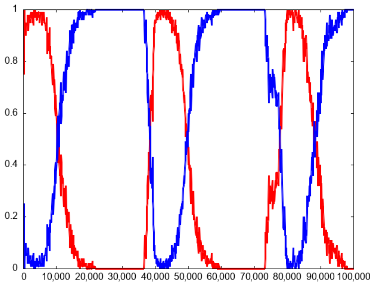
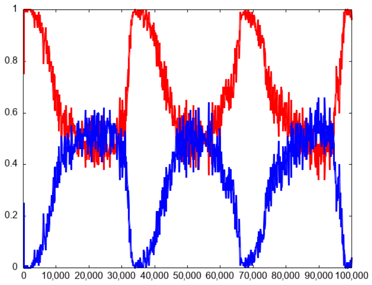
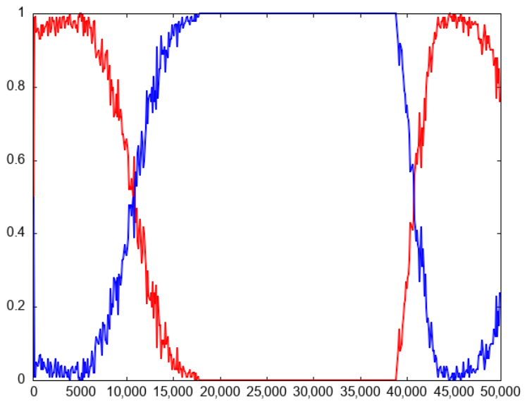
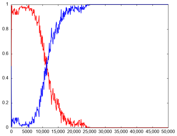
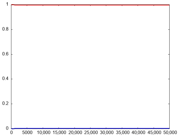
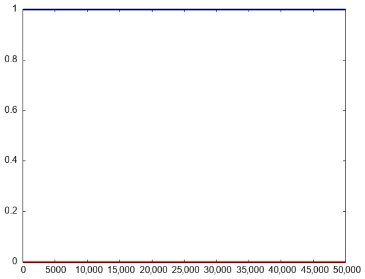
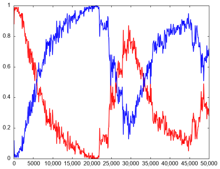
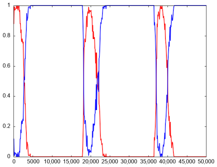
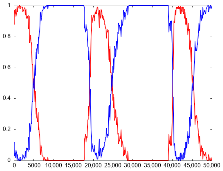
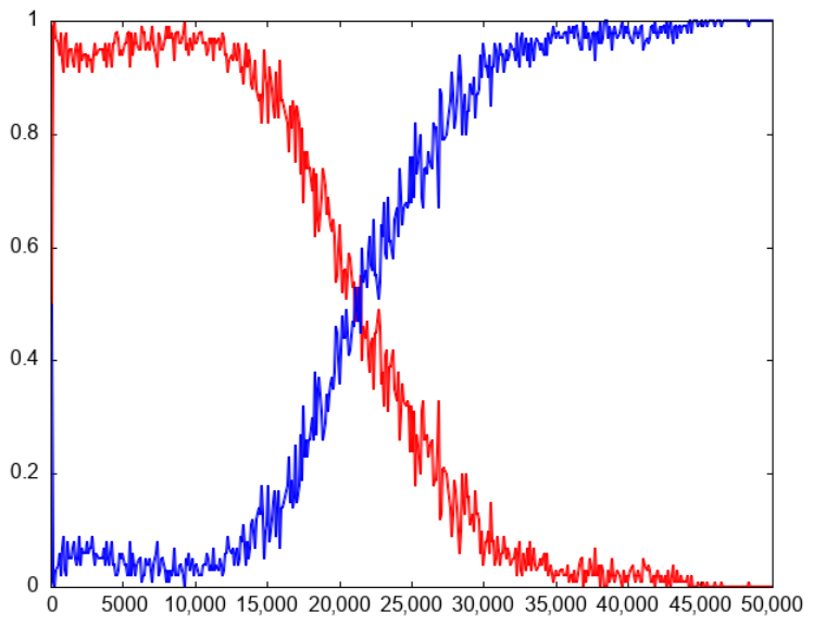
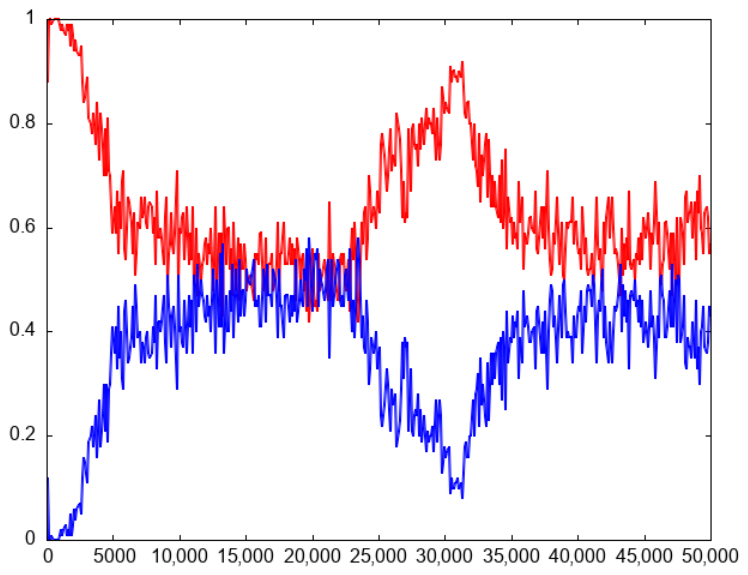
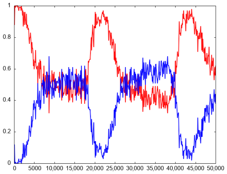
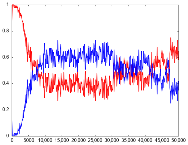
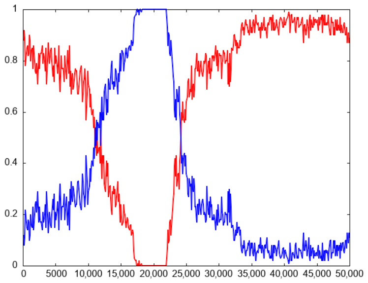
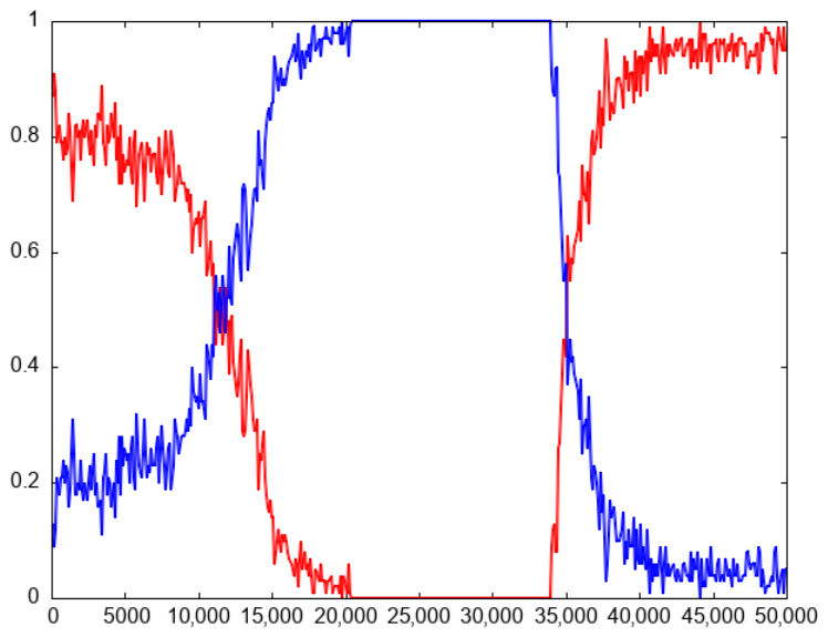
To support our claim of the imprecision of diversity-based measures for exploration and exploitation experimentally, we developed a variant of an EA that generates a new solution in the parent’s vicinity using a small mutation step. We take an extra step to ensure that the newly generated solution is always in the parent’s neighborhood (in the same attraction basin as the parent). By definition, we are always exploiting the search space. However, when exploration and exploitation are quantified using the XPL% and XPT% diversity-based equations, the algorithm is always classified as being in the exploration phase due to the high population diversity (Figure 1). This is a contradiction, since it is clear that we are only exploiting the search space (Figure 2). This example shows, in an extreme case, how imprecise XPL% and XPT% measures can be, contrary to the findings in [53]. Therefore, we advise researchers to avoid using indirect measures for exploration and exploitation.
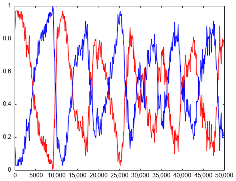
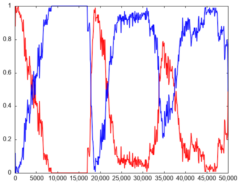
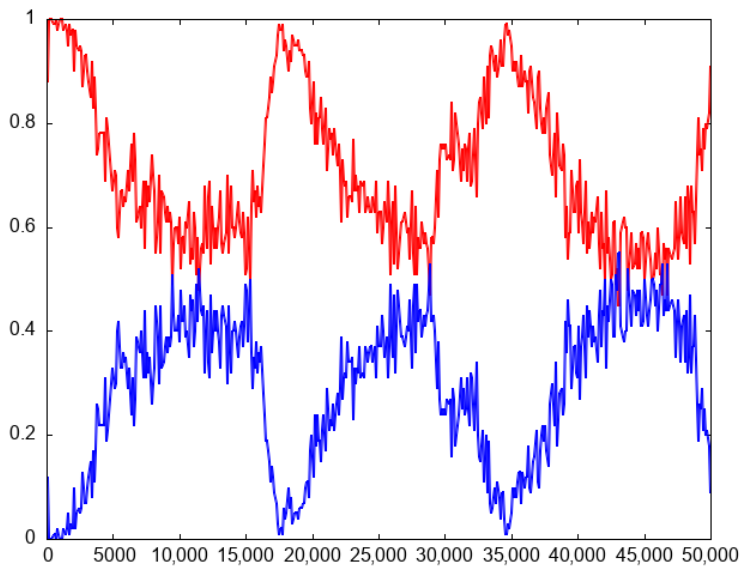
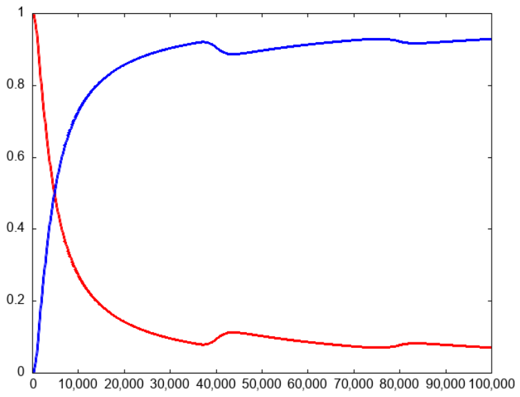
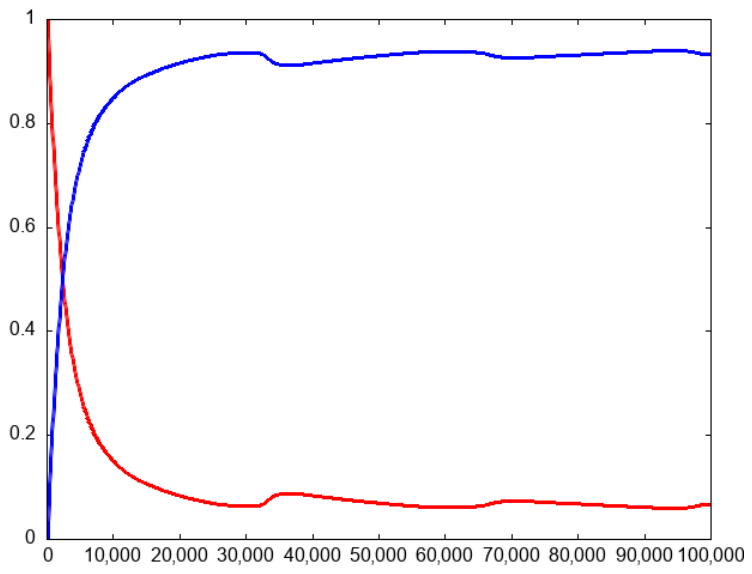
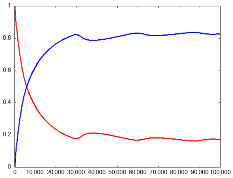
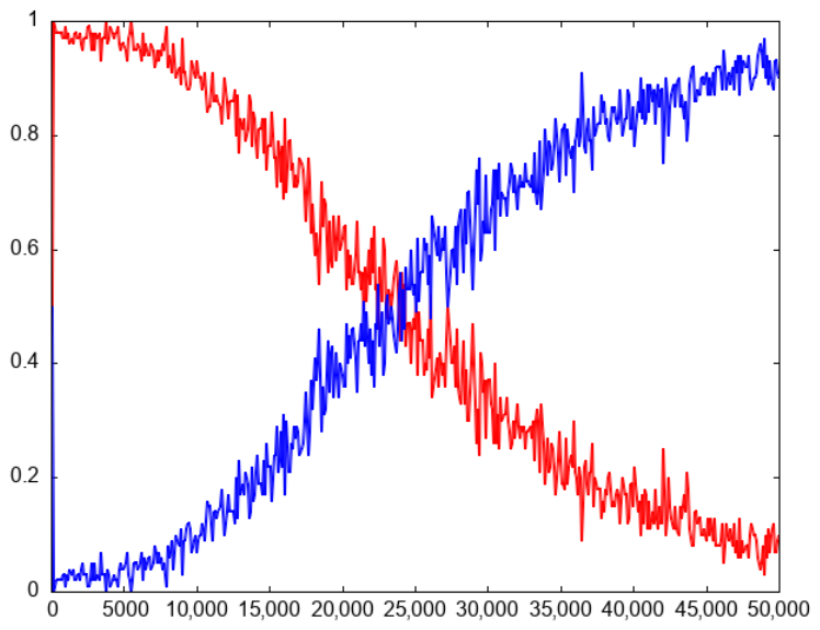
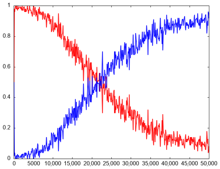
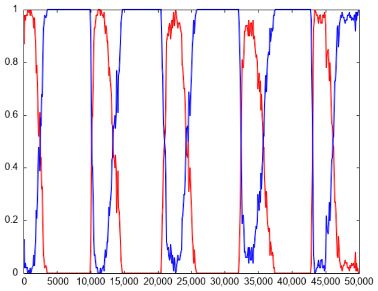
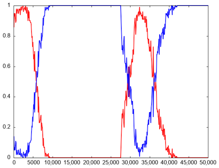
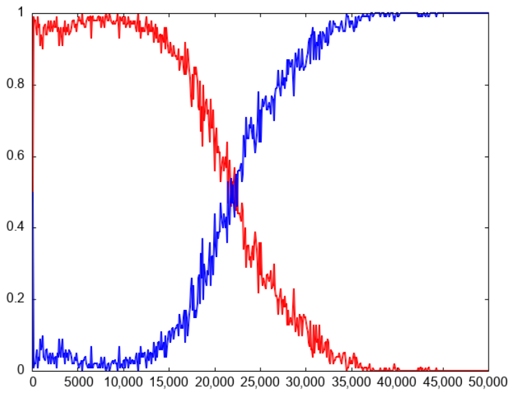
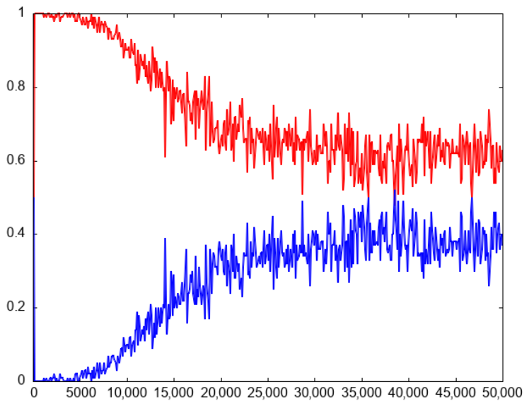
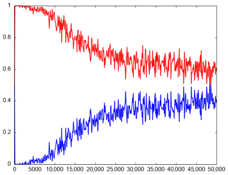
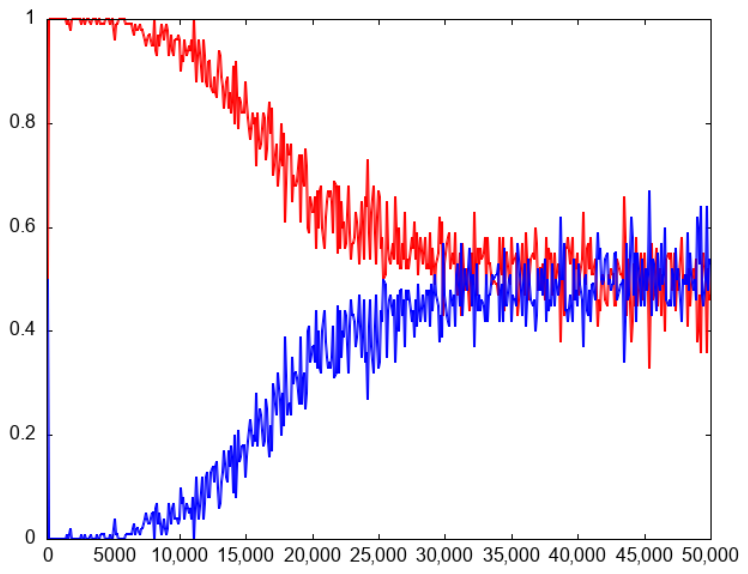
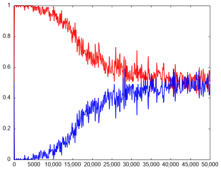
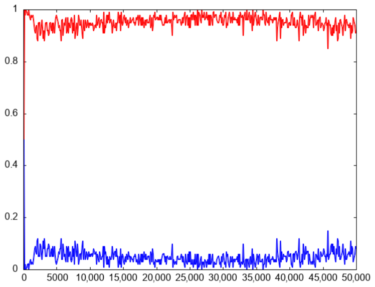
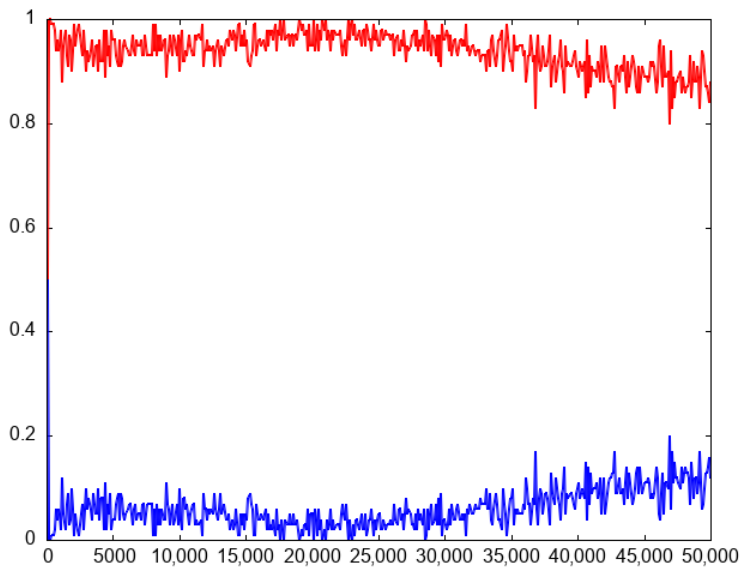
Figure 3, Figure 4, Figure 5, Figure 6, Figure 7 and Figure 8 compare our measures of exploration and exploitation with those based on diversity, further demonstrating the differences between the two approaches on the ABC. The graphs in Figure 3, Figure 5, and Figure 7 look very similar, since they are based on diversity, which declines gradually.

4. Results

To provide a meaningful assessment of the exploration and exploitation behavior of the ABC algorithm, the test suite was deliberately composed of both classical benchmark functions and more challenging benchmark problems with diverse landscape characteristics. The Rastrigin, Ackley, and Griewank functions were selected as they are well-established baseline problems that are used widely in the evaluation of metaheuristic optimizers. These functions exhibit different forms of multimodality, non-separability, and interaction between variables, allowing for a transparent and interpretable analysis of algorithmic behavior on canonical optimization landscapes. In addition, three functions from the CEC 2017 benchmark [55] were included to extend the evaluation to more complex and realistic scenarios. Specifically, F03 represents a highly multimodal landscape, F10 is a hybrid function combining multiple sub-functions with distinct properties, and F20 is a composition function that integrates several basic functions into a single, highly irregular search space. Together, these problems capture a broad spectrum of difficulty levels and landscape features, enabling a more comprehensive investigation of how the control parameter influences the balance between exploration and exploitation under increasing problem complexity. Regarding ABC’s control parameters, a full factorial design has been applied with the following settings that explore the ABC’s behavior under different resource constraints:
  • l i m = { 0 , K , 100 , 250 , 750 , } , where K = S N 2 D ;
  • S N = { 24 , 50 , 100 } ;
  • M F E = { 50 , 000 ; 100 , 000 ; 250 , 000 } ;
  • D = { 5 , 10 , 30 } .
As such, the number of different scenarios was 162 ( 6 × 3 × 3 × 3 ), with 10 independent runs, due to the CRS4EAs (Chess Rating System for Evolutionary algorithms) method, which is appropriate when only a small number of independent runs are available [56]. The local step size ϵ in the local search was as follows: Rastrigin ( ϵ = 0.01 ), Ackley ( ϵ = 0.006 ), and Griewank ( ϵ = 0.12 ), and for F03, F10, and F20 ( ϵ = 0.02 ).
Due to an immense amount of data, only representative graphs of exploration (successful, failed, deceptive, successful rejection) and exploitation (successful, unsuccessful) are shown in the continuation. A summary of the amounts of different types of exploration and exploitation over all problems and for all different control parameter settings (except l i m i t = ) is shown in Table 1. A small standard deviation (e.g., Ackley D = 5 ) indicates that the amounts of different types of exploration and exploitation are stable across all the different parameter settings. For example, the portion of successful exploration is 15 % , failed exploration is 14 % , deceptive exploration is 5 % , and successful rejection is 66 % , regardless of the different control parameter settings. Similarly, this is the case for different types of exploitation (successful exploitation is 20 % , unsuccessful exploitation is 80 % ). A large standard deviation indicates that the balance between exploration and exploitation depends heavily on the control parameter setting (e.g., Ackley D = 30 where exploration is 32 % ± 24 % and exploitation is 68 % ± 24 % ). From Table 1 it can also be observed that the exploration for F03, F10, and F20 is very high, between 70 % and 95 % , while the ratio of exploration to exploitation for the Rastrigin, Ackley, and Griewank problems is distributed more evenly. For Griewank D = 5 , it is 49 % : 51 % .
By examining the exploration and exploitation capabilities of ABC, the following conclusions can be derived from Table 1:
  • Successful rejection is high, above 50 % .
  • Deceptive exploration is not problematic, and is usually below 4 % .
  • Successful exploration is low, between 2 % and 20 % .
  • The amount of failed exploration is usually higher than successful exploration, between 5 % and 40 % .
  • Successful exploitation is low, between 5 % and 25 % .
  • Unsuccessful exploitation is high, between 75 % and 95 % .
Although these conclusions are descriptive, in our opinion, the ratios between the different types of exploration and exploitation are even more important (Table 2). The ratio between successful exploration and deceptive exploration showed that the amount of successful exploration was always higher than that of deceptive exploration, indicating that it moved more often to better than to worse attraction basins, and deceptive exploration was not problematic. This ratio was exceptionally high for D = 30 . On the other hand, the ratio between successful exploration and failed exploration was mixed, and more often, the amount of failed exploration was higher than the amount of successful exploration. This is especially problematic, since better attraction basins have been found but rejected due to greedy survival selection. Again, this ratio was always higher for D = 30 than for D = 5 and D = 10 . The ratio between desired exploration (successful exploration and successful rejection) and undesired exploration (failed exploration and deceptive exploration) was always very high due to a high amount of successful rejection. This ratio was extremely low for F 03 ( D = 5 ) and F 10 ( D = 5 ). The ratio between successful exploration and successful exploitation showed that the amount of successful exploitation was mostly higher than that of successful exploration, which was the desired behavior, as the global optimum could be reached mostly by the exploitation of a neighborhood. Only in a few cases was the amount of successful exploration higher (or almost equal) than the amount of successful exploitation ( F 03 ( D = 30 ) and F 10 ( D = 30 )). The ratio between successful and unsuccessful exploitation was, surprisingly, very low, indicating that searching the neighborhood with existing equations is often not efficient.
The results in Table 1 show a bird’s-eye view of the exploration and exploitation capabilities of ABC on specific problems. It would be interesting to delve deeper and examine the exploration and exploitation graphs for specific problems and control parameter settings through different stages of the evolutionary run. In Figure 9, Figure 10, Figure 11, Figure 12, Figure 13, Figure 14, Figure 15, Figure 16, Figure 17, Figure 18, Figure 19, Figure 20, Figure 21, Figure 22, Figure 23, Figure 24, Figure 25, Figure 26, Figure 27, Figure 28, Figure 29, Figure 30, Figure 31, Figure 32, Figure 33, Figure 34, Figure 35, Figure 36, Figure 37, Figure 38, Figure 39 and Figure 40, we examine the differences between l i m i t = 100 and l i m i t = 750 , as well as between S N = 24 and S N = 100 when M F E = 50 , 000 . For the selected problems, we were interested in the differences in exploration/exploitation behavior when the scout bee phase was triggered more ( l i m i t = 100 ) and less frequently ( l i m i t = 750 ) for a small population ( S N = 24 ) and a larger population ( S N = 100 ).
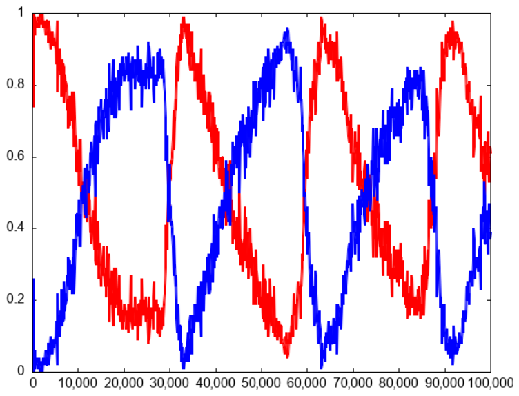
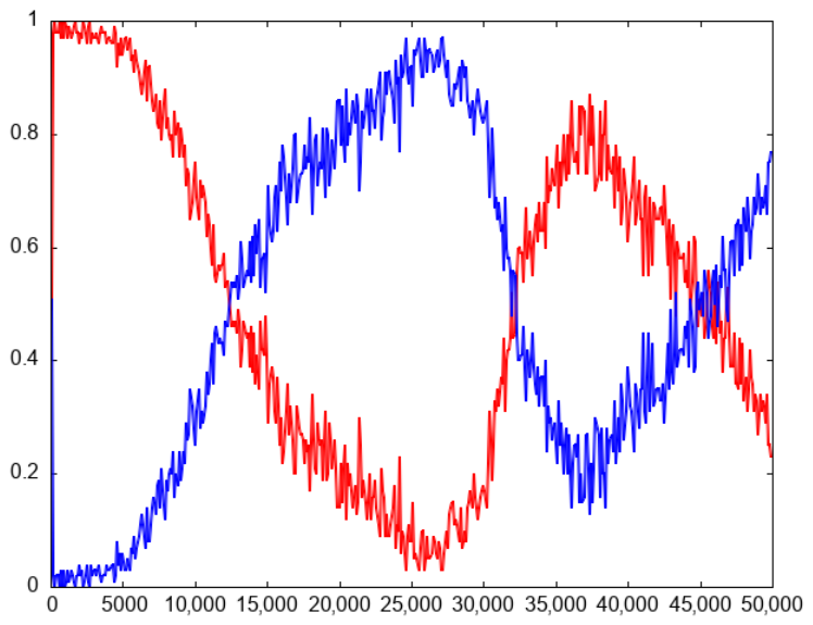
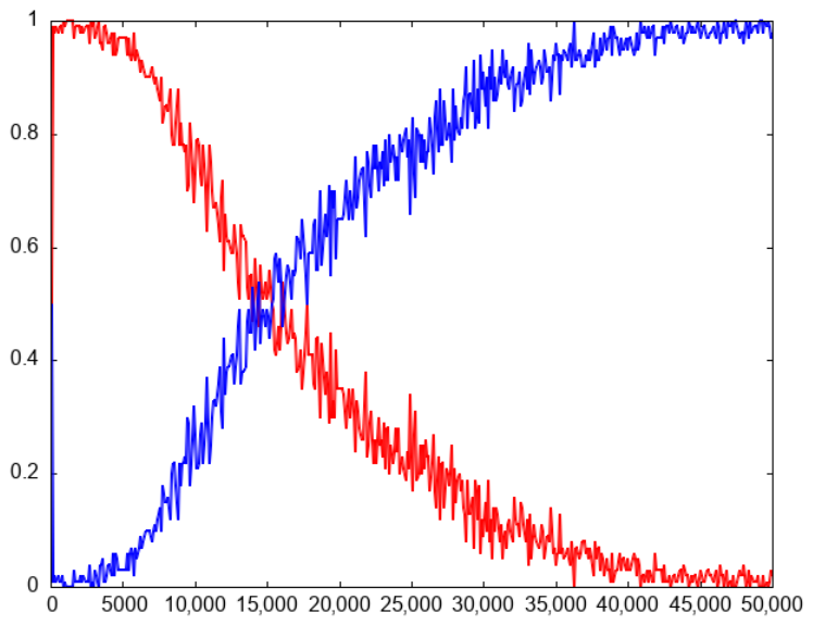
The results for the Rastrigin optimization problem are shown in Figure 9, Figure 10, Figure 11, Figure 12, Figure 13, Figure 14, Figure 15 and Figure 16. Comparing Figure 9 and Figure 10, the effect of the scout bee phase is clearly visible. The increase in exploration (red line) occurs in waves, with unsuccessful trials exceeding l i m i t . When l i m i t is small, l i m i t = 100 , the number of waves is bigger than when l i m i t = 750 . With an increase in population size, from S N = 24 to S N = 100 , we can observe that the amount of exploitation increased, since, at most, one new solution was generated in the scout bee phase (exploration zone), while the new solutions generated in the employed and onlooker bee phases were generated mainly in the exploitation zone (Figure 11 and Figure 12). The previously clearly visible waves are now only observable in Figure 11. In all four examples the amount of exploitation (blue line) is larger than the amount of exploration (red line). When the dimension is increased from D = 5 to D = 10 , from Figure 13, Figure 14, Figure 15 and Figure 16, we can observe that the waves are still visible for a small population ( S N = 24 ), while Figure 15 and Figure 16 are similar to Figure 12.
The results for the Ackley optimization problem are shown in Figure 17, Figure 18, Figure 19, Figure 20, Figure 21, Figure 22, Figure 23 and Figure 24, and the conclusions are very similar to those of the Rastrigin optimization problem.
The results for the Griewank optimization problem are shown in Figure 25, Figure 26, Figure 27, Figure 28, Figure 29, Figure 30, Figure 31 and Figure 32. It is interesting how ABC’s behavior adapted to the new problem, leading to increased exploration. The ratio between exploration and exploitation for D = 5 is 49 % : 51 % . Waves are still observable for the small population size S N = 24 .
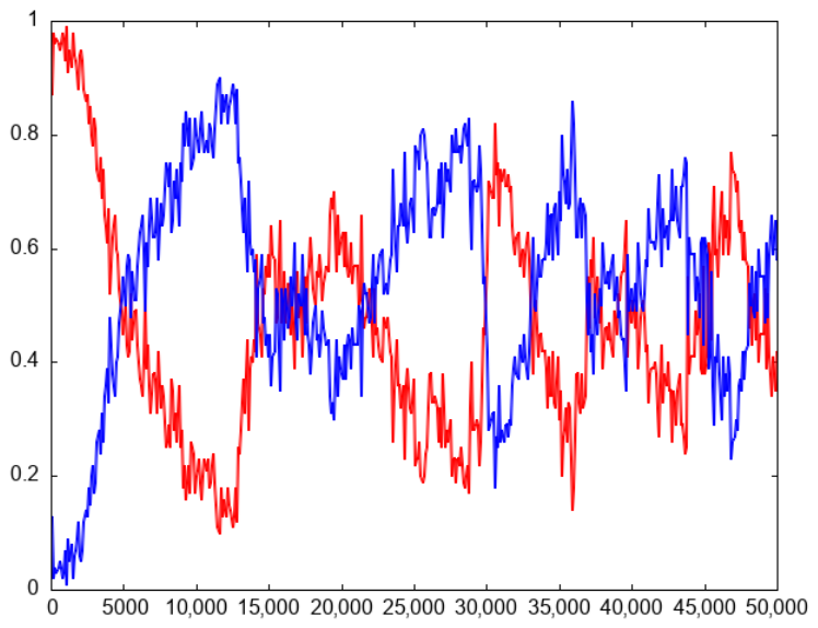
The optimization problems F03, F10 and F20 are more difficult than the previously tested problems. Their exploration/exploitation behavior is very similar. Therefore, graphs are presented only for the F03 problem. From Figure 33, Figure 34, Figure 35, Figure 36, Figure 37, Figure 38, Figure 39 and Figure 40, we can observe that exploration prevails over exploitation. For a small population ( S N = 24 and D = 5 ), the wave from the scout bee phase is still visible (Figure 33 and Figure 34). In all other cases, the amount of exploration is overwhelming, and the ratio between exploration and exploitation is around 90 % : 10 % , indicating that solutions generated in the employed and onlooker bee phases are mainly in the exploration zone.
From Figure 9, Figure 10, Figure 11, Figure 12, Figure 13, Figure 14, Figure 15, Figure 16, Figure 17, Figure 18, Figure 19, Figure 20, Figure 21, Figure 22, Figure 23, Figure 24, Figure 25, Figure 26, Figure 27, Figure 28, Figure 29, Figure 30, Figure 31, Figure 32, Figure 33, Figure 34, Figure 35, Figure 36, Figure 37, Figure 38, Figure 39 and Figure 40, we might expect there to be a direct relationship between the performance and exploration/exploitation curves. However, when exploration is performed primarily, there is no guarantee that a region with a better solution will be discovered and accepted. Similarly, when exploitation is performed primarily, there is no guarantee of fitness improvements. Note that failed exploration, successful rejection and unsuccessful exploitation do not improve solutions. The amount of exploitation and exploration might be high, but there will be no improvements if the aforementioned exploration/exploitation types occur. It is essential to know the proportions of successful, failed, and deceptive exploration and successful rejection, as well as successful and unsuccessful exploitation.
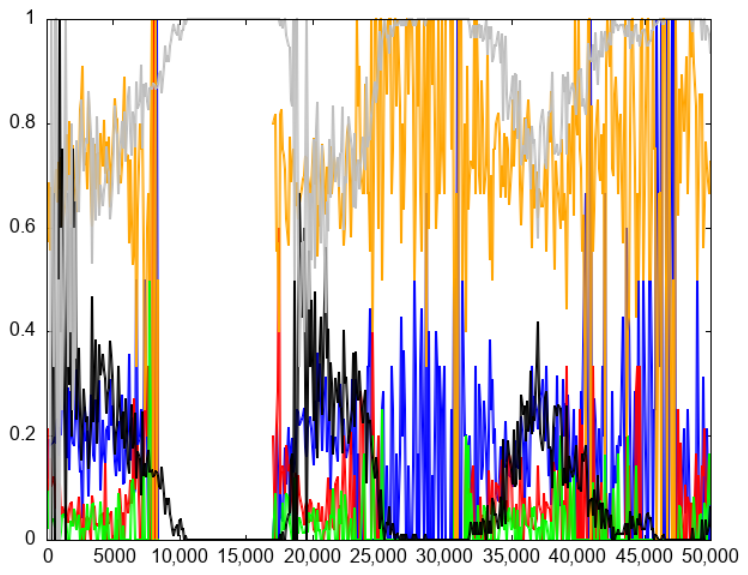
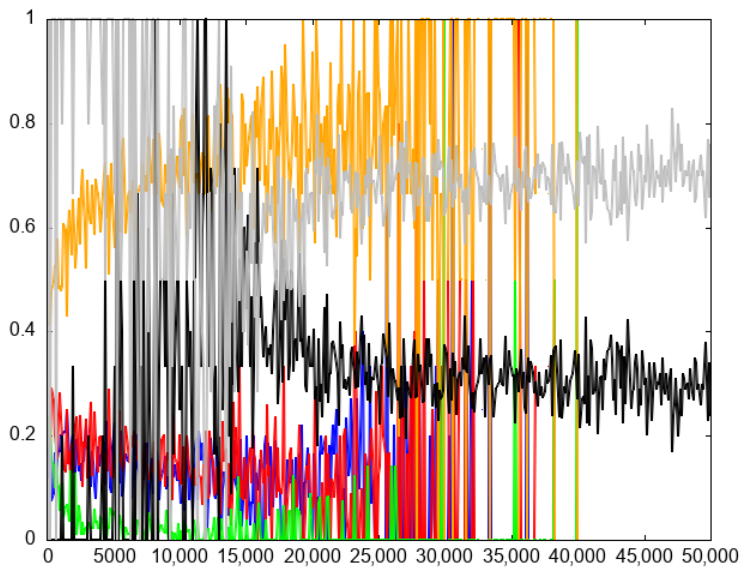
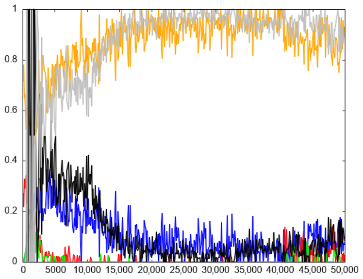
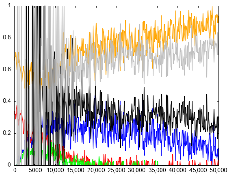
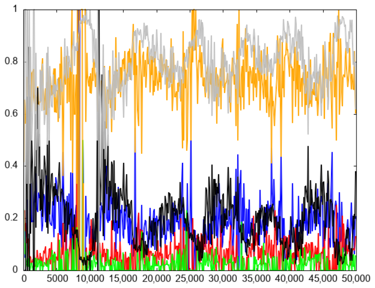
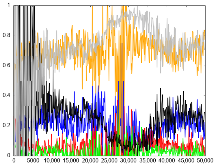
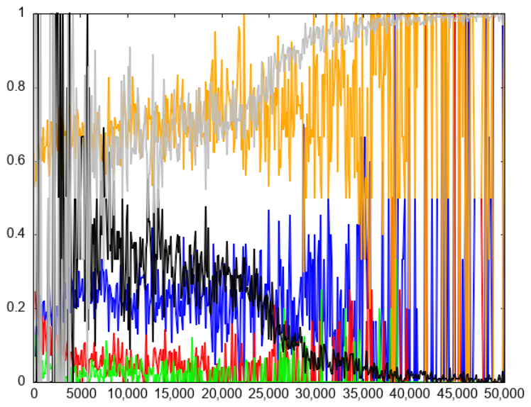
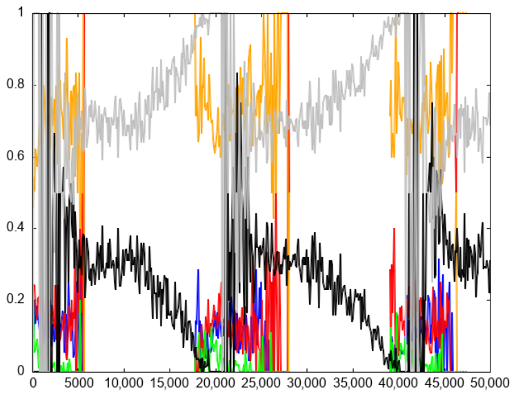
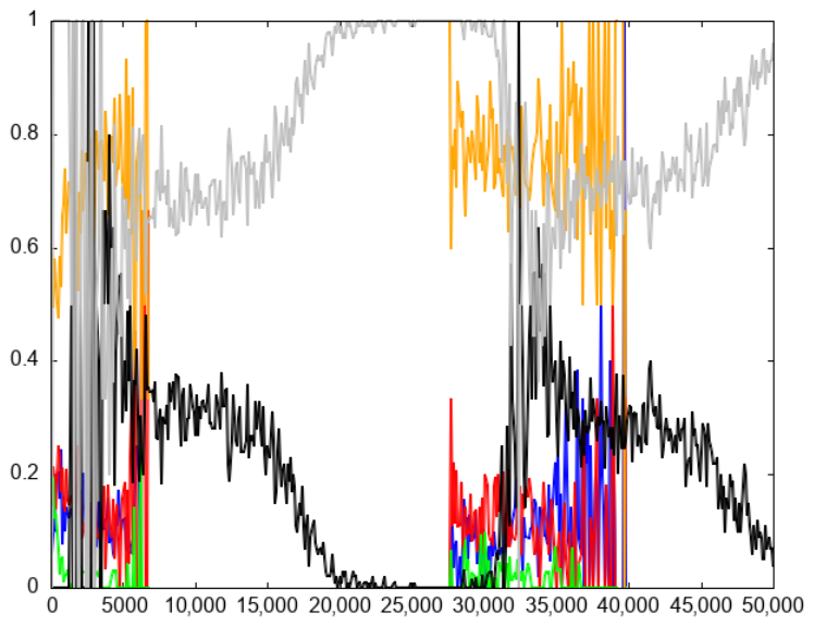
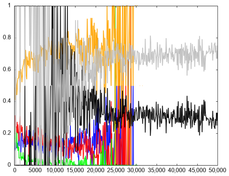
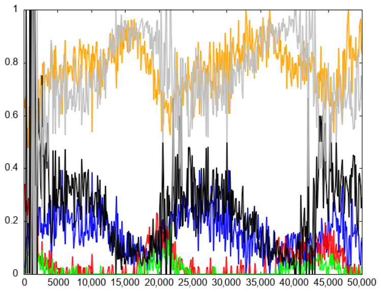
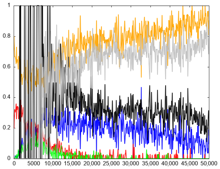
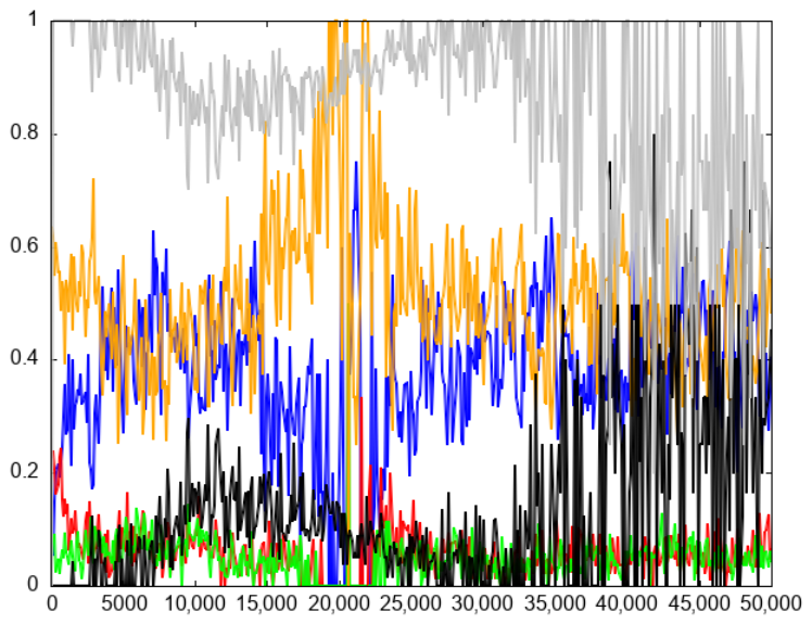
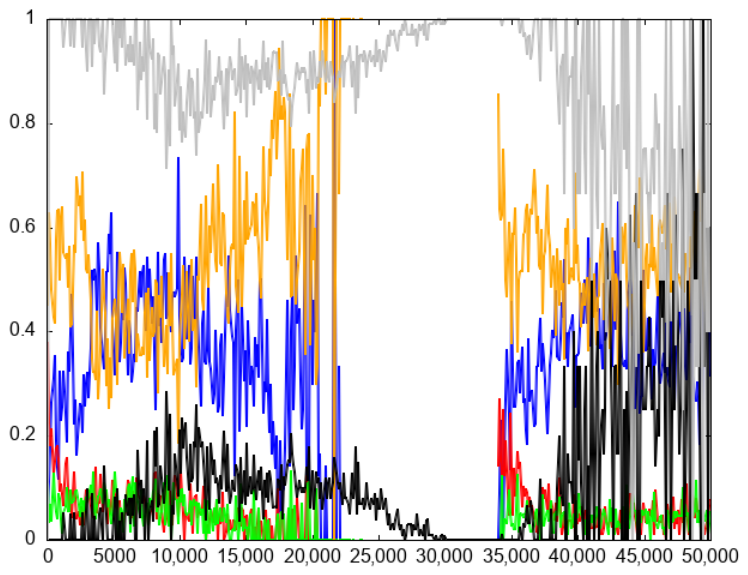
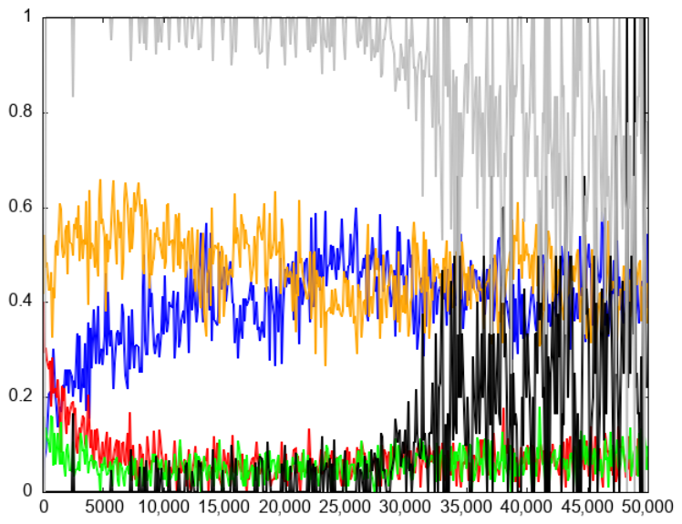
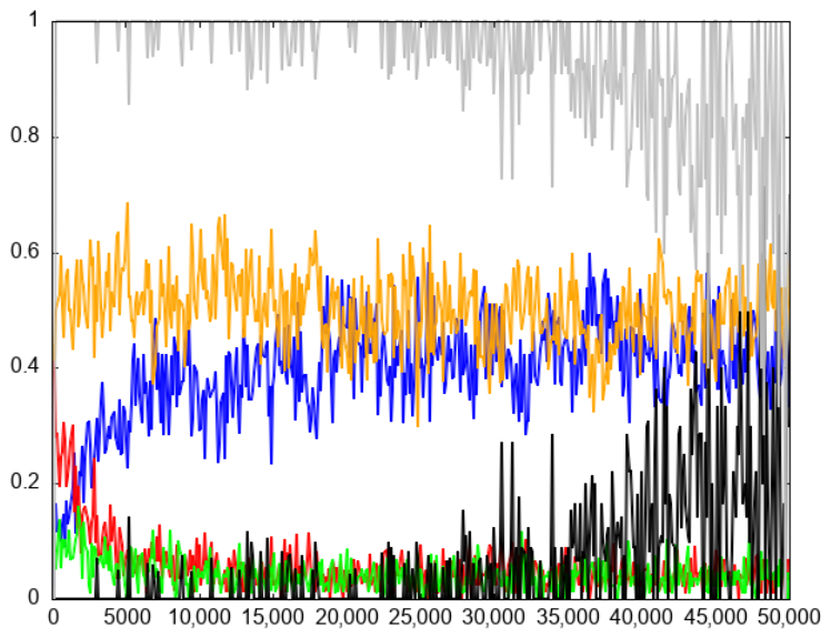
Figure 41, Figure 42, Figure 43 and Figure 44 show the occurrence of different types of exploration and exploitation and their amounts for the Rastrigin problem D = 5 . It can be observed that successful rejection (orange line) prevails over other types of exploration. ABC often finds another region with a worse attractor (local optimum) than the current region. Since the solution is also worse than the current parent solution, it is rejected due to greedy survival selection. The amount of deceptive exploration (green line), where a worse region is accepted, is minimal (around 3 % ) and not problematic. More problematic is the amount of failed exploration (blue line), where a better region is discovered but not accepted due to greedy survival selection. On average, almost every fifth solution in the exploration zone is rejected due to this problem (Table 1). It is also interesting to observe that the amount of failed exploration is almost always larger than successful exploration (red line). On the other hand, the amount of unsuccessful exploitation (gray line) is far larger than successful exploitation (black line). A rough ratio between successful and unsuccessful exploitation is 20 % : 80 % (Table 1). A meticulous reader may find a gap in Figure 42 where only exploitation is performed due to a bigger l i m i t = 750 . However, successful exploitation does not happen during this exploration gap. Only after successful exploration, when better solutions are found, do further improvements occur during the exploitation phase, implying that the previous solution is a local optimum.
Different types of exploration and exploitation on the Ackley problem, D = 10 , show somewhat different behavior than for the Rastrigin problem (Figure 45, Figure 46, Figure 47 and Figure 48). For a small population ( S N = 24 ), exploration comes in waves. The amount of successful exploration is slightly larger than that of failed exploration. An interesting observation from Figure 45 and Figure 46 follows: there is an increase in successful exploration culminating in an increase in successful exploitation. This situation depicts the critical role of exploration and its main purpose: to escape a local optimum, a better region must be found.
Different types of exploration and exploitation on the Griewank problem, D = 10 , are shown in Figure 49, Figure 50, Figure 51 and Figure 52. The main type of exploration is successful rejection, which prevails over other types overwhelmingly. It is interesting that the amount of successful explorations is initially higher than that of failed explorations, implying that a good attraction basin is found quickly. For a small population of S N = 24 and a small l i m i t = 100 , the effect of the scout bee phase can be noticed, with an increased amount of successful exploration (Figure 49), while the amount of successful exploitation is larger than the amount of failed exploration.
Different types of exploration and exploitation on the F03 problem, D = 5 , are shown in Figure 53, Figure 54, Figure 55 and Figure 56. The amount of failed exploration (the blue line) is on par with the successful rejection (the orange line) and is considered very problematic. A better region is found, but is rejected due to greedy survival selection. Another problematic issue is deceptive exploration (the green line), which is on par with successful exploration (the red line). Furthermore, in the beginning, the exploitation is not successful and only increases in later stages. All these observations imply a more difficult landscape.
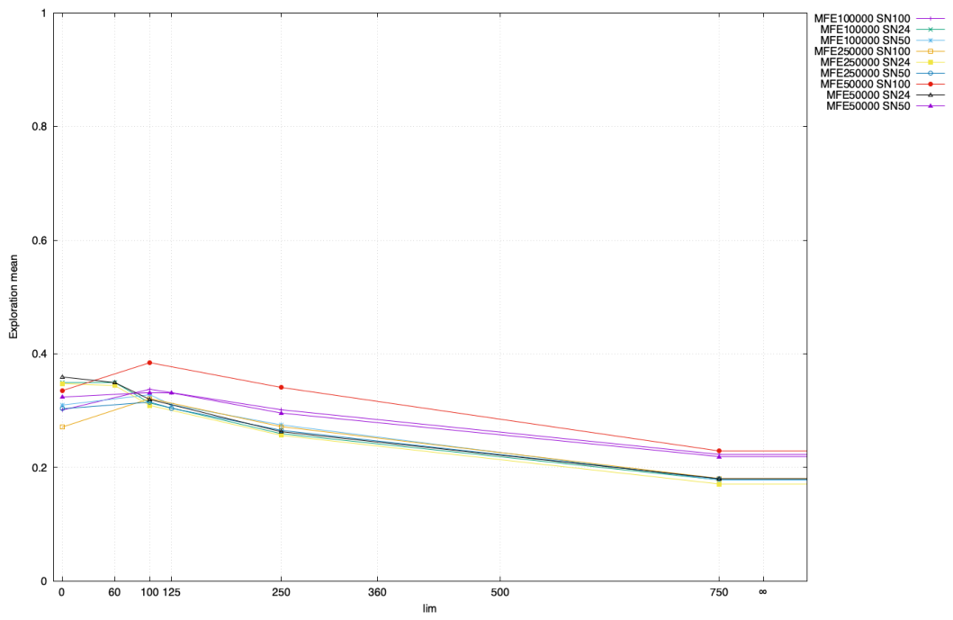
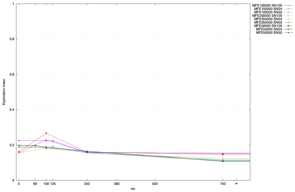
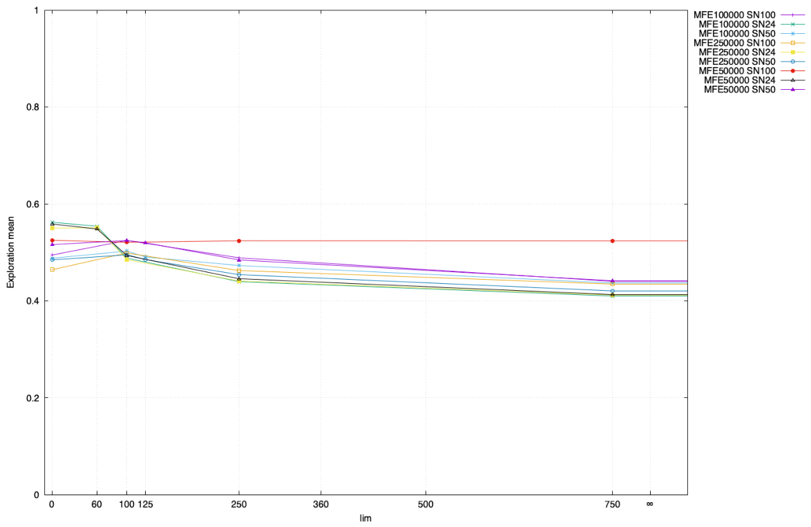
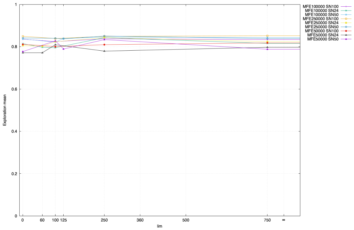
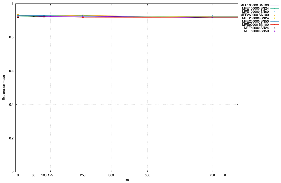
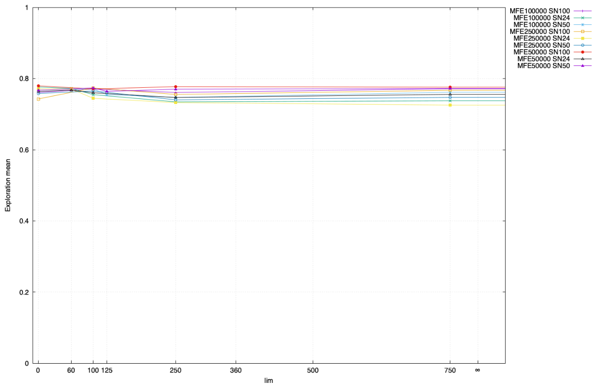
The influence of the control parameter l i m i t on exploration is shown in Figure 57, Figure 58, Figure 59, Figure 60, Figure 61 and Figure 62. For the simple optimization problems (Rastrigin, Ackley, Griewank), there is a clear trend: by increasing the l i m i t , the amount of exploration drops significantly (roughly by 10%). On these problems, the scout bee phase is the main source for the exploration of the search space. By increasing the limit, the scout bee phase no longer activates often. As a consequence, ABC spends less time on exploration. However, it is clear that the employed and onlooker bee phases contribute to the exploration as well.
For the more complex problems (F03, F10, F20), increasing l i m i t had little impact on the amount of exploration. By increasing l i m i t , the scout bee phase was indeed not activated often. However, the employed and onlooker bee phases generated many solutions in the exploration zone, without affecting the different settings of the control parameter l i m i t . Hence, the ruggedness of the fitness landscape culminated in complex attraction basins.

5. Conclusions

Exploration and exploitation are the cornerstones of every search algorithm. Until now, exploration and exploitation have been measured mostly indirectly for EAs using diversity- or entropy-based measures. In this paper, we have shown empirically that these indirect measures are imprecise by developing an EA that exploits the search space by definition. A new solution is always generated in the neighborhood of the parent solution. Although the algorithm was always in the exploitation zone, the diversity-based measure reported 100% exploration because the population was highly diverse. Researchers are advised to stop using imprecise indirect measures for exploration and exploitation. The other major shortcoming of diversity- and entropy-based measures for exploration and exploitation is their inability to measure exploration and exploitation at the individual level. They can only measure exploration and exploitation at the population level indirectly. As such, these measures cannot differentiate between the different types of exploration and exploitation. It is not only important that the EA is in the exploration (exploitation) zone; an algorithm’s ability to move to a region (attraction basin) with a better optimum, or to improve a neighborhood solution, is also very important. In this paper, we discussed four different types of exploration: successful, failed, deceptive, and successful rejection. We also introduced two types of exploitation: successful and unsuccessful.
Based on our newly developed attraction basin-based exploration and exploitation measures, the ABC algorithm has been investigated to assess its exploration and exploitation capabilities. Previously, many researchers [18,19,20,21,22,23,24,25,26] have reported the weak exploitation capability of ABC, while the work in [27] also pointed to its weak exploration capability. However, these claims were not based on direct measurements of exploration and exploitation, but on assumptions about which zone a newly generated solution fell into, and on the observation that the scout bee phase was triggered rarely when the control parameter l i m i t was set to high values. While the scout bee phase indeed contributes to exploration, the line is blurred between exploration and exploitation between the employed and onlooker bee phases. Especially for hard problems (F03, F10, F20), many new solutions generated in the employed and onlooker bee phases contributed towards exploration.
To summarize, the most important observations about ABC’s exploration and exploitation capabilities are:
  • The amount of deceptive exploration is small and not problematic.
  • Often, the amount of failed exploration is higher than the amount of successful exploration. This is especially problematic, since better attraction basins have been found but rejected due to greedy survival selection.
  • The ratio between successful and unsuccessful exploitation is surprisingly very low, indicating that searching the neighborhood with existing equations is often not efficient.
While conducting experiments using ABC, several important insights emerged regarding exploration and exploitation:
  • Measuring exploration and exploitation alone is not sufficient and cannot be related directly to metaheuristics performance. Two different metaheuristics might have the same ratio between exploration and exploitation, yet very different performance. Hence, identification is needed of the different types of exploration and exploitation. Important is the ratio between desired and undesired explorations, as well as between successful and unsuccessful exploitation, although a general pattern of exploration and exploitation is descriptive and important (see the patterns in Figure 9, Figure 10, Figure 11, Figure 12, Figure 13, Figure 14, Figure 15, Figure 16, Figure 17, Figure 18, Figure 19, Figure 20, Figure 21, Figure 22, Figure 23, Figure 24, Figure 25, Figure 26, Figure 27, Figure 28, Figure 29, Figure 30, Figure 31, Figure 32, Figure 33, Figure 34, Figure 35, Figure 36, Figure 37, Figure 38, Figure 39 and Figure 40).
  • Despite exploring the search space, it is not guaranteed that a better region has been discovered. This situation is depicted by successful rejection, deceptive exploration and failed exploration. In the latter case, a better region is discovered, but it is abandoned due to greedy survival selection.
  • Despite exploiting the search space, it is not guaranteed that a better solution has been discovered, due to unsuccessful sampling of the neighborhood. This situation is depicted by unsuccessful exploitation.
  • The amount of successful exploitation should be higher than that of successful exploration, as the global optimum can be reached mostly by exploitation of a neighborhood.
  • A combination of successful rejection and unsuccessful exploitation depicts algorithm stagnation.
  • When an increase in successful exploration precedes an increase in successful exploitation, investment in exploration has paid off.
  • Unsuccessful exploitation is undesired, since the neighborhood has been searched, but no better solution has been found.
In our future work, we would like to investigate the differences and similarities in exploration and exploitation across different EAs (e.g., GA, GWO, and PSO), including adaptive strategies (e.g., adaptive Differential Evolution and adaptive ABC), and to measure the effects of different selection methods on exploration and exploitation. By using our direct attraction basin-based measure for exploration and exploitation, we can also verify several claims about the algorithm’s performance. For example, the work in [20] claimed that the newly developed EABC achieved an ideal balance between exploration and exploitation. Without measuring exploration and exploitation directly, such a claim is hard to verify. Once explicit control of exploration and exploitation is understood well in single-objective optimization, further research is needed to apply explicit exploration measures to constrained, noisy, multi-objective, and dynamic optimization problems. Yet another direction of research is to investigate which approaches lead to fewer undesired explorations (failed and deceptive), as well as to determine how to control exploration and exploitation in EAs.

Author Contributions

Conceptualization, J.J. and M.M.; methodology, J.J., M.R., L.M. and M.M.; software, J.J.; validation, M.R., L.M. and M.M.; investigation, J.J., M.R., L.M. and M.M.; writing—original draft preparation, J.J., M.R., L.M. and M.M.; writing—review and editing, J.J., M.R., L.M. and M.M.; visualization, J.J.; supervision, M.M. All authors have read and agreed to the published version of the manuscript.

Funding

This research was funded by the Slovenian Research and Innovation Agency, Grant Numbers P2-0041 (B) and P2-0114.

Data Availability Statement

The source code of the experiment is available at https://github.com/UM-LPM/exploration-and-exploitation (accessed on 16 April 2026).

Conflicts of Interest

The authors declare no conflicts of interest.

References

  1. Karaboga, D.; Basturk, B. On the performance of artificial bee colony (ABC) algorithm. Appl. Soft Comput. 2008, 8, 687–697. [Google Scholar] [CrossRef] [Scilit]
  2. Akay, B.; Karaboga, D. A modified Artificial Bee Colony algorithm for real-parameter optimization. Inf. Sci. 2012, 192, 120–142. [Google Scholar] [CrossRef] [Scilit]
  3. Tsai, C.; Chiang, M. Handbook of Metaheuristic Algorithms: From Fundamental Theories to Advanced Applications; Elsevier: Amsterdam, The Netherlands, 2023. [Google Scholar]
  4. Rajwar, K.; Deep, K.; Das, S. An exhaustive review of the metaheuristic algorithms for search and optimization: Taxonomy, applications, and open challenges. Artif. Intell. Rev. 2023, 56, 13187–13257. [Google Scholar] [CrossRef] [Scilit]
  5. Ding, Z.; Huang, M.; Lu, Z. Structural damage detection using artificial bee colony algorithm with hybrid search strategy. Swarm Evol. Comput. 2016, 28, 1–13. [Google Scholar] [CrossRef] [Scilit]
  6. Jesenik, M.; Trbušić, M. The approach of using a horizontally layered soil model for Inhomogeneous soil, by taking into account the deeper layers of the soil, and determining the model’s parameters using evolutionary methods. Appl. Sci. 2025, 15, 1420. [Google Scholar] [CrossRef] [Scilit]
  7. Jesenik, M.; Mernik, M.; Trlep, M. Determination of a Hysteresis Model Parameters with the Use of Different Evolutionary Methods for an Innovative Hysteresis Model. Mathematics 2020, 8, 201. [Google Scholar] [CrossRef] [Scilit]
  8. Li, G.; Liu, C.; Wu, L.; Xiao, W. A mixing algorithm of ACO and ABC for solving path planning of mobile robot. Appl. Soft Comput. 2023, 148, 110868. [Google Scholar] [CrossRef] [Scilit]
  9. Jesenik, M.; Ravber, M.; Trbušić, M. Innovative Approach for the Determination of a DC Motor’s and Drive’s Parameters Using Evolutionary Methods and Different Measured Current and Angular Speed Responses. Mathematics 2024, 12, 42. [Google Scholar] [CrossRef] [Scilit]
  10. Gülsün, B.; Aydin, M.R. Optimizing a Machine Learning Algorithm by a Novel Metaheuristic Approach: A Case Study in Forecasting. Mathematics 2024, 12, 3921. [Google Scholar] [CrossRef] [Scilit]
  11. Touafek, N.; Tayeb, F.B.S.; Ladj, A.; Baghdadi, R. Advanced Optimization of Flowshop Scheduling with Maintenance, Learning and Deteriorating Effects Leveraging Surrogate Modeling Approaches. Mathematics 2025, 13, 2381. [Google Scholar] [CrossRef] [Scilit]
  12. Civicioglu, P.; Besdok, E. A conceptual comparison of the Cuckoo-search, particle swarm optimization, differential evolution and artificial bee colony algorithms. Artif. Intell. Rev. 2013, 39, 315–346. [Google Scholar] [CrossRef] [Scilit]
  13. Aslan, S. A comparative study between artificial bee colony (ABC) algorithm and its variants on big data optimization. Memetic Comput. 2020, 12, 129–150. [Google Scholar] [CrossRef] [Scilit]
  14. Mernik, M.; Liu, S.H.; Karaboga, D.; Črepinšek, M. On clarifying misconceptions when comparing variants of the Artificial Bee Colony Algorithm by offering a new implementation. Inf. Sci. 2015, 291, 115–127. [Google Scholar] [CrossRef] [Scilit]

  15. Črepinšek, M.; Liu, S.H.; Mernik, M. Exploration and Exploitation in Evolutionary Algorithms: A Survey. ACM Comput. Surv. 2013, 45, 35. [Google Scholar] [CrossRef] [Scilit]
  16. Eiben, A.E.; Smith, J.E. Introduction to Evolutionary Computing; Natural Computing Series; Springer: Berlin/Heidelberg, Germany, 2003. [Google Scholar]
  17. Michalewicz, Z. Genetic Algorithms + Data Structures = Evolution Programs; Springer: Berlin/Heidelberg, Germany, 1999. [Google Scholar]
  18. Zhu, G.; Kwong, S. Gbest-guided artificial bee colony algorithm for numerical function optimization. Appl. Math. Comput. 2010, 217, 3166–3173. [Google Scholar] [CrossRef] [Scilit]
  19. Gao, W.; Liu, S.; Huang, L. A Novel Artificial Bee Colony Algorithm Based on Modified Search Equation and Orthogonal Learning. IEEE Trans. Cybern. 2013, 43, 1011–1024. [Google Scholar] [CrossRef] [Scilit]
  20. Gao, W.; Liu, S.; Huang, L. Enhancing artificial bee colony algorithm using more information-based search equations. Inf. Sci. 2014, 270, 112–133. [Google Scholar] [CrossRef] [Scilit]
  21. Wang, H.; Wu, Z.; Rahnamayan, S.; Sun, H.; Liu, Y.; Pan, J.S. Multi-strategy ensemble artificial bee colony algorithm. Inf. Sci. 2014, 279, 587–603. [Google Scholar] [CrossRef] [Scilit]
  22. Wang, B. A novel artificial bee colony algorithm based on modified search strategy and generalized opposition-based learning. J. Intell. Fuzzy Syst. 2015, 28, 1023–1037. [Google Scholar] [CrossRef] [Scilit]
  23. Kiran, M.S.; Hakli, H.; Gunduz, M.; Uguz, H. Artificial bee colony algorithm with variable search strategy for continuous optimization. Inf. Sci. 2015, 300, 140–157. [Google Scholar] [CrossRef] [Scilit]
  24. Song, X.; Zhao, M.; Yan, Q.; Xing, S. A high-efficiency adaptive artificial bee colony algorithm using two strategies for continuous optimization. Swarm Evol. Comput. 2019, 50, 100549. [Google Scholar] [CrossRef] [Scilit]
  25. Zhou, X.; Lu, J.; Huang, J.; Zhong, M.; Wang, M. Enhancing artificial bee colony algorithm with multi-elite guidance. Inf. Sci. 2021, 543, 242–258. [Google Scholar] [CrossRef] [Scilit]
  26. Wang, Y.; Jiao, J.; Liu, J.; Xiao, R. A labor division artificial bee colony algorithm based on behavioral development. Inf. Sci. 2022, 606, 152–172. [Google Scholar] [CrossRef] [Scilit]
  27. Singh, A.; Deep, K. Exploration–exploitation balance in Artificial Bee Colony algorithm: A critical analysis. Soft Comput. 2019, 23, 9525–9536. [Google Scholar] [CrossRef] [Scilit]
  28. Veček, N.; Liu, S.H.; Črepinšek, M.; Mernik, M. On the importance of the artificial bee colony control parameter ‘Limit’. Inf. Technol. Control 2017, 46, 566–604. [Google Scholar] [CrossRef] [Scilit]
  29. Alsamia, S.; Koch, E.; Albedran, H.; Ray, R. Adaptive Exploration Artificial Bee Colony for Mathematical Optimization. AI 2024, 5, 2218–2236. [Google Scholar] [CrossRef] [Scilit]
  30. Jerebic, J.; Mernik, M.; Liu, S.H.; Ravber, M.; Baketarić, M.; Mernik, L.; Črepinšek, M. A novel direct measure of exploration and exploitation based on attraction basins. Expert Syst. Appl. 2021, 167, 114353. [Google Scholar] [CrossRef] [Scilit]
  31. Li, M.; Chang, C.; Liu, Z. A discrete artificial bee colony algorithm and its application in flexible flow shop scheduling with assembly and machine deterioration effect. Appl. Soft Comput. 2024, 159, 111593. [Google Scholar] [CrossRef] [Scilit]
  32. Luo, Q.; Rao, Y.; Du, B. An effective discrete artificial bee colony for the rectangular cutting problem with guillotine in transformer manufacturing. Appl. Soft Comput. 2024, 159, 111617. [Google Scholar] [CrossRef] [Scilit]
  33. Yu, Y.; Zhang, F.; Yang, G.; Wang, Y.; Huang, J.; Han, Y. A discrete artificial bee colony method based on variable neighborhood structures for the distributed permutation flowshop problem with sequence-dependent setup times. Swarm Evol. Comput. 2022, 75, 101179. [Google Scholar] [CrossRef] [Scilit]
  34. Soza, C.; Becerra, R.L.; Riff, M.C.; Coello Coello, C.A. Solving timetabling problems using a cultural algorithm. Appl. Soft Comput. 2011, 11, 337–344. [Google Scholar] [CrossRef] [Scilit]
  35. Olorunda, O.; Engelbrecht, A.P. Measuring exploration/exploitation in particle swarms using swarm diversity. In Proceedings of the 2008 IEEE Congress on Evolutionary Computation (IEEE World Congress on Computational Intelligence); IEEE: Piscataway, NJ, USA, 2008; pp. 1128–1134. [Google Scholar]
  36. Cheng, S.; Shi, Y.; Qin, Q.; Zhang, Q.; Bai, R. Population Diversity Maintenance In Brain Storm Optimization Algorithm. J. Artif. Intell. Soft Comput. Res. 2014, 4, 83–97. [Google Scholar] [CrossRef] [Scilit]
  37. Yang, Q.; Chen, W.N.; Deng, J.D.; Li, Y.; Gu, T.; Zhang, J. A Level-Based Learning Swarm Optimizer for Large-Scale Optimization. IEEE Trans. Evol. Comput. 2018, 22, 578–594. [Google Scholar] [CrossRef] [Scilit]
  38. Hussain, K.; Salleh, M.N.M.; Cheng, S.; Shi, Y. On the exploration and exploitation in popular swarm-based metaheuristic algorithms. Neural Comput. Appl. 2019, 31, 7665–7683. [Google Scholar] [CrossRef] [Scilit]
  39. Li, D.; Guo, W.; Lerch, A.; Li, Y.; Wang, L.; Wu, Q. An adaptive particle swarm optimizer with decoupled exploration and exploitation for large scale optimization. Swarm Evol. Comput. 2021, 60, 100789. [Google Scholar] [CrossRef] [Scilit]
  40. Morales-Castañeda, B.; Zaldívar, D.; Cuevas, E.; Fausto, F.; Rodríguez, A. A better balance in metaheuristic algorithms: Does it exist? Swarm Evol. Comput. 2020, 54, 100671. [Google Scholar] [CrossRef] [Scilit]
  41. Liu, S.H.; Mernik, M.; Hrnčič, D.; Črepinšek, M. A parameter control method of evolutionary algorithms using exploration and exploitation measures with a practical application for fitting Sovova’s mass transfer model. Appl. Soft Comput. 2013, 13, 3792–3805. [Google Scholar] [CrossRef] [Scilit]
  42. Popič, J.; Bošković, B.; Brest, J. Improving mutation strategies in differential evolution with a new pbest selection mechanism. Appl. Soft Comput. 2025, 185, 113978. [Google Scholar] [CrossRef] [Scilit]
  43. Malan, K.M.; Engelbrecht, A.P. Fitness Landscape Analysis for Metaheuristic Performance Prediction. In Recent Advances in the Theory and Application of Fitness Landscapes; Richter, H., Engelbrecht, A., Eds.; Springer: Berlin/Heidelberg, Germany, 2014; pp. 103–132. [Google Scholar]
  44. Gonzalez-Fernandez, Y.; Chen, S. Leaders and followers—A new metaheuristic to avoid the bias of accumulated information. In Proceedings of the 2015 IEEE Congress on Evolutionary Computation (CEC); IEEE: Piscataway, NJ, USA, 2015; pp. 776–783. [Google Scholar]
  45. Baketarić, M.; Mernik, M.; Kosar, T. Attraction Basins in Metaheuristics: A Systematic Mapping Study. Mathematics 2021, 9, 3036. [Google Scholar] [CrossRef] [Scilit]
  46. Cotta, C.; Gallardo, J.E.; Mathieson, L.; Moscato, P. Memetic Algorithms: A Contemporary Introduction. In Wiley Encyclopedia of Electrical and Electronics Engineering; John Wiley & Sons, Ltd.: Hoboken, NJ, USA, 2016; pp. 1–15. [Google Scholar]
  47. Neri, F.; Cotta, C.; Moscato, P. Handbook of Memetic Algorithms; Springer: Berlin/Heidelberg, Germany, 2011; Volume 379. [Google Scholar]
  48. Chen, S.; Bolufé-Röhler, A.; Montgomery, J.; Tamayo-Vera, D.; Hendtlass, T. Measuring the Effects of Increasing Dimensionality on Fitness-Based Selection and Failed Exploration. In Proceedings of the 2022 IEEE Congress on Evolutionary Computation (CEC); IEEE: Piscataway, NJ, USA, 2022; pp. 1–8. [Google Scholar]
  49. Ochoa, G.; Tomassini, M.; Vérel, S.; Darabos, C. A Study of NK Landscapes’ Basins and Local Optima Networks. In Proceedings of the 10th Annual Conference on Genetic and Evolutionary Computation; Association for Computing Machinery: New York, NY, USA, 2008; pp. 555–562. [Google Scholar]
  50. Pitzer, E.; Affenzeller, M.; Beham, A. A closer look down the basins of attraction. In Proceedings of the 2010 UK Workshop on Computational Intelligence; IEEE: Piscataway, NJ, USA, 2010; pp. 1–6. [Google Scholar]
  51. Tsang, K.K. Basin of Attraction as a measure of robustness of an optimization algorithm. In Proceedings of the 2018 14th International Conference on Natural Computation, Fuzzy Systems and Knowledge Discovery; IEEE: Piscataway, NJ, USA, 2018; pp. 133–137. [Google Scholar]
  52. Drugan, M.M. Estimating the number of basins of attraction of multi-objective combinatorial problems. J. Comb. Optim. 2019, 37, 1367–1407. [Google Scholar] [CrossRef] [Scilit]
  53. Ferhat, A.; Zitouni, F.; Lakbichi, R.; Limane, A.; Harous, S. Measures of exploration and exploitation rates in MAs: Classification, comparison, and convergence analysis. Memetic Comput. 2025, 17, 37. [Google Scholar] [CrossRef] [Scilit]
  54. Yildizdan, G.; Baykan, Ö.K. A New Hybrid BA_ABC Algorithm for Global Optimization Problems. Mathematics 2020, 8, 1749. [Google Scholar] [CrossRef] [Scilit]
  55. Awad, N.; Ali, M.; Liang, J.; Qu, B.; Suganthan, P.; Definitions, P. Evaluation criteria for the CEC 2017 special session and competition on single objective real-parameter numerical optimization. Technol. Rep. 2016, 9. [Google Scholar]
  56. Veček, N.; Črepinšek, M.; Mernik, M. On the influence of the number of algorithms, problems, and independent runs in the comparison of evolutionary algorithms. Appl. Soft Comput. 2017, 54, 23–45. [Google Scholar] [CrossRef] [Scilit]
Figure 1. XPL% (red line)/XPT% (blue line) based on diversity.
Mathematics 14 01406 g001
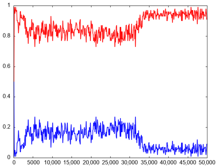
Figure 2. XPL (red line)/XPT (blue line) based on attraction basins.
Mathematics 14 01406 g002
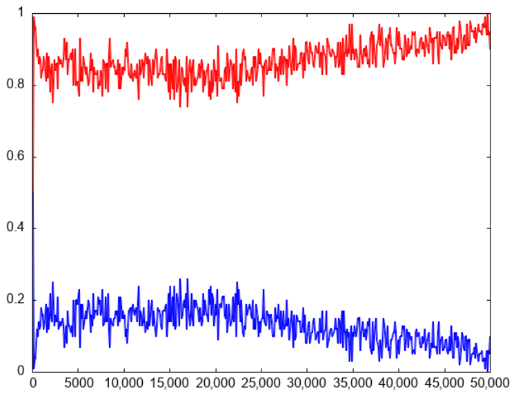
Figure 3. Ackley: XPL% (red line)/XPT% (blue line) based on diversity.
Mathematics 14 01406 g003
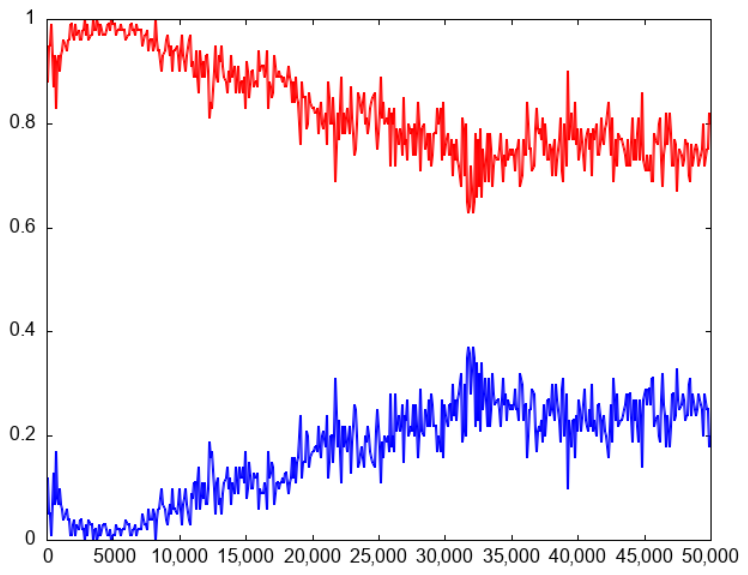
Figure 4. Ackley: XPL (red line)/XPT (blue line) based on attraction basins.
Mathematics 14 01406 g004
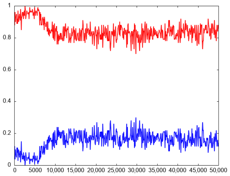
Figure 5. Griewank: XPL% (red line)/XPT% (blue line) based on diversity.
Mathematics 14 01406 g005
Figure 6. Griewank: XPL (red line)/XPT (blue line) based on attraction basins.
Mathematics 14 01406 g006
Figure 7. Rastrigin: XPL% (red line)/XPT% (blue line) based on diversity.
Mathematics 14 01406 g007
Figure 8. Rastrigin: XPL (red line)/XPT (blue line) based on attraction basins.
Mathematics 14 01406 g008
Figure 9. XPL (red line) and XPT (blue line) for the Rastrigin optimization problem ( D = 5 , l i m = 100 , S N = 24 , M F E = 50 , 000 ).
Mathematics 14 01406 g009
Figure 10. XPL (red line) and XPT (blue line) for the Rastrigin optimization problem ( D = 5 , l i m = 750 , S N = 24 , M F E = 50 , 000 ).
Mathematics 14 01406 g010
Figure 11. XPL (red line) and XPT (blue line) for the Rastrigin optimization problem ( D = 5 , l i m = 100 , S N = 100 , M F E = 50 , 000 ).
Mathematics 14 01406 g011
Figure 12. XPL (red line) and XPT (blue line) for the Rastrigin optimization problem ( D = 5 , l i m = 750 , S N = 100 , M F E = 50 , 000 ).
Mathematics 14 01406 g012
Figure 13. XPL (red line) and XPT (blue line) for the Rastrigin optimization problem ( D = 10 , l i m = 100 , S N = 24 , M F E = 50 , 000 ).
Mathematics 14 01406 g013
Figure 14. XPL (red line) and XPT (blue line) for the Rastrigin optimization problem ( D = 10 , l i m = 750 , S N = 24 , M F E = 50 , 000 ).
Mathematics 14 01406 g014
Figure 15. XPL (red line) and XPT (blue line) for the Rastrigin optimization problem ( D = 10 , l i m = 100 , S N = 100 , M F E = 50 , 000 ).
Mathematics 14 01406 g015
Figure 16. XPL (red line) and XPT (blue line) for the Rastrigin optimization problem ( D = 10 , l i m = 750 , S N = 100 , M F E = 50 , 000 ).
Mathematics 14 01406 g016
Figure 17. XPL (red line) and XPT (blue line) for the Ackley optimization problem ( D = 5 , l i m = 100 , S N = 24 , M F E = 50 , 000 ).
Mathematics 14 01406 g017
Figure 18. XPL (red line) and XPT (blue line) for the Ackley optimization problem ( D = 5 , l i m = 750 , S N = 24 , M F E = 50 , 000 ).
Mathematics 14 01406 g018
Figure 19. XPL (red line) and XPT (blue line) for the Ackley optimization problem ( D = 5 , l i m = 100 , S N = 100 , M F E = 50 , 000 ).
Mathematics 14 01406 g019
Figure 20. XPL (red line) and XPT (blue line) for the Ackley optimization problem ( D = 5 , l i m = 750 , S N = 100 , M F E = 50 , 000 ).
Mathematics 14 01406 g020
Figure 21. XPL (red line) and XPT (blue line) for the Ackley optimization problem ( D = 10 , l i m = 100 , S N = 24 , M F E = 50 , 000 ).
Mathematics 14 01406 g021
Figure 22. XPL (red line) and XPT (blue line) for the Ackley optimization problem ( D = 10 , l i m = 750 , S N = 24 , M F E = 50 , 000 ).
Mathematics 14 01406 g022
Figure 23. XPL (red line) and XPT (blue line) for the Ackley optimization problem ( D = 10 , l i m = 100 , S N = 100 , M F E = 50 , 000 ).
Mathematics 14 01406 g023
Figure 24. XPL (red line) and XPT (blue line) for the Ackley optimization problem ( D = 10 , l i m = 750 , S N = 100 , M F E = 50 , 000 ).
Mathematics 14 01406 g024
Figure 25. XPL (red line) and XPT (blue line) for the Griewank optimization problem ( D = 5 , l i m = 100 , S N = 24 , M F E = 50 , 000 ).
Mathematics 14 01406 g025
Figure 26. XPL (red line) and XPT (blue line) for the Griewank optimization problem ( D = 5 , l i m = 750 , S N = 24 , M F E = 50 , 000 ).
Mathematics 14 01406 g026
Figure 27. XPL (red line) and XPT (blue line) for the Griewank optimization problem ( D = 5 , l i m = 100 , S N = 100 , M F E = 50 , 000 ).
Mathematics 14 01406 g027
Figure 28. XPL (red line) and XPT (blue line) for the Griewank optimization problem ( D = 5 , l i m = 750 , S N = 100 , M F E = 50 , 000 ).
Mathematics 14 01406 g028
Figure 29. XPL (red line) and XPT (blue line) for the Griewank optimization problem ( D = 10 , l i m = 100 , S N = 24 , M F E = 50 , 000 ).
Mathematics 14 01406 g029
Figure 30. XPL (red line) and XPT (blue line) for the Griewank optimization problem ( D = 10 , l i m = 750 , S N = 24 , M F E = 50 , 000 ).
Mathematics 14 01406 g030
Figure 31. XPL (red line) and XPT (blue line) for the Griewank optimization problem ( D = 10 , l i m = 100 , S N = 100 , M F E = 50 , 000 ).
Mathematics 14 01406 g031
Figure 32. XPL (red line) and XPT (blue line) for the Griewank optimization problem ( D = 10 , l i m = 750 , S N = 100 , M F E = 50 , 000 ).
Mathematics 14 01406 g032
Figure 33. XPL (red line) and XPT (blue line) for the F03 optimization problem ( D = 5 , l i m = 100 , S N = 24 , M F E = 50 , 000 ).
Mathematics 14 01406 g033
Figure 34. XPL (red line) and XPT (blue line) for the F03 optimization problem ( D = 5 , l i m = 750 , S N = 24 , M F E = 50 , 000 ).
Mathematics 14 01406 g034
Figure 35. XPL (red line) and XPT (blue line) for the F03 optimization problem ( D = 5 , l i m = 100 , S N = 100 , M F E = 50 , 000 ).
Mathematics 14 01406 g035
Figure 36. XPL (red line) and XPT (blue line) for the F03 optimization problem ( D = 5 , l i m = 750 , S N = 100 , M F E = 50 , 000 ).
Mathematics 14 01406 g036
Figure 37. XPL (red line) and XPT (blue line) for the F03 optimization problem ( D = 10 , l i m = 100 , S N = 24 , M F E = 50 , 000 ).
Mathematics 14 01406 g037
Figure 38. XPL (red line) and XPT (blue line) for the F03 optimization problem ( D = 10 , l i m = 750 , S N = 24 , M F E = 50 , 000 ).
Mathematics 14 01406 g038
Figure 39. XPL (red line) and XPT (blue line) for the F03 optimization problem ( D = 10 , l i m = 100 , S N = 100 , M F E = 50 , 000 ).
Mathematics 14 01406 g039
Figure 40. XPL (red line) and XPT (blue line) for the F03 optimization problem ( D = 10 , l i m = 750 , S N = 100 , M F E = 50 , 000 ).
Mathematics 14 01406 g040
Figure 41. Exploration and exploitation types for the Rastrigin optimization problem ( D = 5 , l i m = 100 , S N = 24 , M F E = 50 , 000 ).
Mathematics 14 01406 g041
Figure 42. Exploration and exploitation types for the Rastrigin optimization problem ( D = 5 , l i m = 750 , S N = 24 , M F E = 50 , 000 ).
Mathematics 14 01406 g042
Figure 43. Exploration and exploitation types for the Rastrigin optimization problem ( D = 5 , l i m = 100 , S N = 100 , M F E = 50 , 000 ).
Mathematics 14 01406 g043
Figure 44. Exploration and exploitation types for the Rastrigin optimization problem ( D = 5 , l i m = 750 , S N = 100 , M F E = 50 , 000 ).
Mathematics 14 01406 g044
Figure 45. Exploration and exploitation types for the Ackley optimization problem ( D = 10 , l i m = 100 , S N = 24 , M F E = 50 , 000 ).
Mathematics 14 01406 g045
Figure 46. Exploration and exploitation types for the Ackley optimization problem ( D = 10 , l i m = 750 , S N = 24 , M F E = 50 , 000 ).
Mathematics 14 01406 g046
Figure 47. Exploration and exploitation types for the Ackley optimization problem ( D = 10 , l i m = 100 , S N = 100 , M F E = 50 , 000 ).
Mathematics 14 01406 g047
Figure 48. Exploration and exploitation types for the Ackley optimization problem ( D = 10 , l i m = 750 , S N = 100 , M F E = 50 , 000 ).
Mathematics 14 01406 g048
Figure 49. Exploration and exploitation types for the Griewank optimization problem ( D = 10 , l i m = 100 , S N = 24 , M F E = 50 , 000 ).
Mathematics 14 01406 g049
Figure 50. Exploration and exploitation types for the Griewank optimization problem ( D = 10 , l i m = 750 , S N = 24 , M F E = 50 , 000 ).
Mathematics 14 01406 g050
Figure 51. Exploration and exploitation types for the Griewank optimization problem ( D = 10 , l i m = 100 , S N = 100 , M F E = 50 , 000 ).
Mathematics 14 01406 g051
Figure 52. Exploration and exploitation types for the Griewank optimization problem ( D = 10 , l i m = 750 , S N = 100 , M F E = 50 , 000 ).
Mathematics 14 01406 g052
Figure 53. Exploration and exploitation types for the F03 optimization problem ( D = 5 , l i m = 100 , S N = 24 , M F E = 50 , 000 ).
Mathematics 14 01406 g053
Figure 54. Exploration and exploitation types for the F03 optimization problem ( D = 5 , l i m = 750 , S N = 24 , M F E = 50 , 000 ).
Mathematics 14 01406 g054
Figure 55. Exploration and exploitation types for the F03 optimization problem ( D = 5 , l i m = 100 , S N = 100 , M F E = 50 , 000 ).
Mathematics 14 01406 g055
Figure 56. Exploration and exploitation types for the F03 optimization problem ( D = 5 , l i m = 750 , S N = 100 , M F E = 50 , 000 ).
Mathematics 14 01406 g056
Figure 57. Influence of l i m i t on the Rastrigin optimization problem ( D = 5 ).
Mathematics 14 01406 g057
Figure 58. Influence of l i m i t on the Ackley optimization problem ( D = 5 ).
Mathematics 14 01406 g058
Figure 59. Influence of l i m i t on the Griewank optimization problem ( D = 5 ).
Mathematics 14 01406 g059
Figure 60. Influence of l i m i t on the F03 optimization problem ( D = 5 ).
Mathematics 14 01406 g060
Figure 61. Influence of l i m i t on the F10 optimization problem ( D = 5 ).
Mathematics 14 01406 g061
Figure 62. Influence of l i m i t on the F20 optimization problem ( D = 5 ).
Mathematics 14 01406 g062
Table 1. Exploration and exploitation summary metrics of ABC for selected problems.
ProblemDSEFEDESR SE xpt UE xpt XPLXPT
Rastrigin50.0702
± 0.0014
0.1875
± 0.0084
0.0316
± 0.0010
0.7107
± 0.0101
0.1469
± 0.0354
0.8531
± 0.0354
0.2896
± 0.0573
0.7104
± 0.0573
Rastrigin100.0567
± 0.0029
0.1700
± 0.0108
0.0147
± 0.0013
0.7586
± 0.0146
0.1685
± 0.0373
0.8315
± 0.0373
0.2678
± 0.0438
0.7322
± 0.0438
Rastrigin300.0986
± 0.0147
0.0746
± 0.0662
0.0033
± 0.0028
0.8235
± 0.0636
0.2211
± 0.0794
0.7789
± 0.0794
0.4409
± 0.1855
0.5591
± 0.1855
Ackley50.1525
± 0.0039
0.1410
± 0.0045
0.0481
± 0.0014
0.6584
± 0.0094
0.1995
± 0.0371
0.8005
± 0.0371
0.1713
± 0.0344
0.8287
± 0.0344
Ackley100.1546
± 0.0079
0.1139
± 0.0066
0.0312
± 0.0022
0.7003
± 0.0162
0.2214
± 0.0355
0.7786
± 0.0355
0.1702
± 0.0363
0.8298
± 0.0363
Ackley300.1932
± 0.0234
0.0717
± 0.0633
0.0197
± 0.0172
0.7154
± 0.0583
0.2713
± 0.0583
0.7287
± 0.0583
0.3225
± 0.2439
0.6775
± 0.2439
Griewank50.0412
± 0.0095
0.1210
± 0.0251
0.0140
± 0.0033
0.8238
± 0.0376
0.1235
± 0.0289
0.8765
± 0.0289
0.4880
± 0.0424
0.5120
± 0.0424
Griewank100.0562
± 0.0160
0.1282
± 0.0286
0.0201
± 0.0057
0.7954
± 0.0498
0.1382
± 0.0419
0.8618
± 0.0419
0.3851
± 0.0381
0.6149
± 0.0381
Griewank300.2087
± 0.0367
0.0454
± 0.0406
0.0056
± 0.0049
0.7403
± 0.0511
0.2384
± 0.0736
0.7616
± 0.0736
0.3684
± 0.1665
0.6316
± 0.1665
F0350.0502
± 0.0120
0.4273
± 0.0197
0.0442
± 0.0096
0.4783
± 0.0115
0.0811
± 0.0135
0.9189
± 0.0135
0.8217
± 0.0232
0.1783
± 0.0232
F03100.0557
± 0.0150
0.1134
± 0.0135
0.0167
± 0.0045
0.8142
± 0.0281
0.2190
± 0.0512
0.7810
± 0.0512
0.9319
± 0.0268
0.0681
± 0.0268
F03300.0920
± 0.0437
0.0323
± 0.0289
0.0090
± 0.0080
0.8667
± 0.0379
0.0549
± 0.0096
0.9451
± 0.0096
0.9268
± 0.0049
0.0732
± 0.0049
F1050.0213
± 0.0092
0.4336
± 0.0171
0.0185
± 0.0077
0.5266
± 0.0035
0.0662
± 0.0211
0.9338
± 0.0211
0.9243
± 0.0039
0.0757
± 0.0039
F10100.0384
± 0.0144
0.1390
± 0.0227
0.0060
± 0.0017
0.8166
± 0.0109
0.0745
± 0.0145
0.9255
± 0.0145
0.9296
± 0.0254
0.0704
± 0.0254
F10300.0680
± 0.0263
0.0148
± 0.0161
0.0024
± 0.0024
0.9148
± 0.0243
0.0687
± 0.0233
0.9313
± 0.0233
0.9431
± 0.0035
0.0569
± 0.0035
F2050.0135
± 0.0072
0.2882
± 0.0084
0.0086
± 0.0041
0.6897
± 0.0130
0.0789
± 0.0312
0.9211
± 0.0312
0.7613
± 0.0135
0.2387
± 0.0135
F20100.0150
± 0.0066
0.2966
± 0.0072
0.0065
± 0.0028
0.6819
± 0.0118
0.0746
± 0.0253
0.9254
± 0.0253
0.6959
± 0.0089
0.3041
± 0.0089
F20300.0469
± 0.0218
0.0491
± 0.0587
0.0025
± 0.0030
0.9016
± 0.0519
0.0634
± 0.0160
0.9366
± 0.0160
0.9440
± 0.0235
0.0560
± 0.0235
Table 2. Ratios derived from the exploration and exploitation summary metrics of ABC for selected problems.
ProblemDSE/DESE/FE DE xpl / UE xpl SE/ SE xpt SE xpt / UE xpt
Rastrigin52.22150.37443.56410.47790.1722
Rastrigin103.85710.33354.41420.33650.2026
Rastrigin3029.87881.321711.83700.44600.2839
Ackley53.17051.08164.28820.76440.2492
Ackley104.95511.35735.89180.69830.2844
Ackley309.80712.69469.94090.71210.3723
Griewank52.94290.34056.40740.33360.1409
Griewank102.79600.43845.74240.40670.1604
Griewank3037.26794.596918.60780.87540.3130
F0351.13570.11751.12090.61900.0883
F03103.33530.49126.68640.25430.2804
F033010.22222.848323.21311.67580.0581
F1051.15140.04911.21190.32180.0709
F10106.40000.27635.89660.51540.0805
F103028.33334.594657.13950.98980.0738
F2051.56980.04682.36930.17110.0857
F20102.30770.05062.29920.20110.0806
F203018.76000.955218.38180.73970.0677
Disclaimer/Publisher’s Note: The statements, opinions and data contained in all publications are solely those of the individual author(s) and contributor(s) and not of MDPI and/or the editor(s). MDPI and/or the editor(s) disclaim responsibility for any injury to people or property resulting from any ideas, methods, instructions or products referred to in the content.