Multi-Scale Decomposition and Autocorrelation Modeling for Classical and Machine Learning-Based Time Series Forecasting

Abstract

Environmental time series, such as near-surface air temperature, exhibit strong multi-scale structure and persistent autocorrelation. Accurate forecasting therefore requires careful consideration of both temporal scale separation and serial dependence. In this study, we evaluate a unified framework that integrates Kolmogorov–Zurbenko (KZ) filtering with two classes of models: (i) classical regression with Cochrane–Orcutt autocorrelation correction, and (ii) an autocorrelation-adjusted Long Short-Term Memory (LSTM) network that learns an embedded correlation coefficient ($\rho$). All models are assessed using standardized meteorological predictors of T2M under walk-forward validation. The LSTM trained on raw predictors shows moderate performance (RMSE = 0.73, $R^2=0.46$, DW = 0.79), which improves after KZ filtering (RMSE = 0.59, $R^2=0.63$, DW = 1.84). Classical regression applied to KZ-decomposed predictors and corrected using the Cochrane–Orcutt procedure achieves substantially higher accuracy (RMSE = 0.41, $R^2=0.89$, DW $\approx 2.0$), outperforming the LSTM in both predictive precision and residual behavior. Visual diagnostics further confirm tighter predicted–actual alignment and near-white residuals in the classical models, whereas the LSTM retains small systematic deviations even after filtering. Overall, the results demonstrate that addressing multi-scale structures and autocorrelation had a greater impact than increasing model complexity. Integrating spectral decomposition with autocorrelation correction thus produces more reliable, statistically valid forecasts, demonstrating that classical regression with KZ filtering can surpass LSTM models in both accuracy and interpretability. These findings emphasize the value of combining time series–aware pre-processing with both traditional and neural network approaches for environmental prediction.

1. Introduction

Time-series forecasting frequently encounters challenges arising from seasonality, noise, and autocorrelation. To address these issues, various decomposition techniques—such as Seasonal-Trend Decomposition using Loess (STL) [1], Empirical Mode Decomposition (EMD) [2], Wavelet Decomposition [3], and the Kolmogorov–Zurbenko (KZ) filter [4,5]—are employed to separate long-term trends, seasonal cycles, and short-term fluctuations. Among these, the KZ filter has gained considerable attention in climatological and hydrological studies due to its ability to isolate multi-scale variations using simple moving-average iterations [4,6,7]. By decomposing a time series into interpretable components, the KZ filter allows researchers to better understand and model underlying temporal structures, but most existing studies apply it primarily for descriptive analysis rather than as part of a statistically robust predictive framework [8]. Accurate forecasting of surface air temperature is vital across multiple scientific and operational domains. In climatology, it enables the detection of long-term warming trends and the quantification of interannual variability [9]. In hydrology, temperature strongly influences evapotranspiration, streamflow, and groundwater recharge processes [10]. Beyond the environmental sciences, sectors such as energy management, agriculture, and public health rely on reliable temperature forecasts for planning and adaptation strategies [10,11]. Given its central role in Earth system processes, improving the predictive accuracy of temperature remains both a scientific necessity and a societal priority. Despite the wide adoption of decomposition-based modeling, existing studies often overlook whether residual autocorrelation persists in the decomposed components, and classical regression frameworks are rarely combined with multi-scale decomposition [12,13]. Persistent autocorrelation can bias regression coefficients, inflate significance tests, and compromise model interpretability. Consequently, there is a clear methodological gap: most prior work does not integrate multi-scale decomposition with formal autocorrelation correction in a unified predictive modeling framework.

Classical econometric techniques, including the Durbin–Watson test and correction procedures such as Cochrane–Orcutt and Prais–Winsten [14,15], provide well-established means of addressing serial correlation. However, these methods have largely been applied to raw, non-decomposed datasets, limiting their effectiveness in capturing multi-scale variability. Furthermore, related fields such as hydrology and communications have demonstrated the utility of combining statistical corrections with data decomposition or deep learning for improved forecasting [8,16], yet such integrated approaches remain scarce in temperature prediction studies.

Machine learning (ML) methods, particularly Long Short-Term Memory (LSTM) networks, have also achieved notable success in hydrological and climatic forecasting [7,11,16,17,18]. LSTMs are well-suited for sequential data, capturing long-range dependencies through gated memory mechanisms and flexible nonlinear representations, with performance governed by architectural and training hyperparameters such as network depth, hidden units, learning rate, and regularization strategies [19]. Their effectiveness has also been demonstrated beyond environmental sciences, including applications in communications and traffic forecasting [16], where LSTM models often outperform traditional linear benchmarks such as ARIMA when strong nonlinearities and long-memory effects are present. Nevertheless, most ML-based forecasting studies rely primarily on model flexibility to implicitly learn temporal dependence, without explicitly addressing key structural characteristics of environmental time series, such as multi-scale variability and residual autocorrelation [20]. This limits interpretability and statistical rigor, as residual diagnostics beyond standard accuracy measures (e.g., RMSE, MAE, $R^2$) are rarely evaluated. Consequently, direct comparison between ML and regression-based models is complicated in settings where seasonal cycles, long-term trends, and short-term fluctuations coexist.

In this study, we address these gaps by integrating multi-scale decomposition via the KZ filter with both classical regression (OLS, Ridge, Lasso) and LSTM models, incorporating explicit autocorrelation correction at each walk-forward step. For linear models, the Cochrane–Orcutt procedure is applied sequentially to decomposed components, while in LSTM models, an autoregressive parameter $\rho$ is jointly optimized with network weights. This unified framework enables a comprehensive evaluation of predictive performance and statistical interpretability across both methodological paradigms. By explicitly combining decomposition with autocorrelation correction, we target limitations identified in prior studies and demonstrate a robust strategy for forecasting complex environmental time series.

2. Materials and Methods

2.1. Overall Methodological Framework

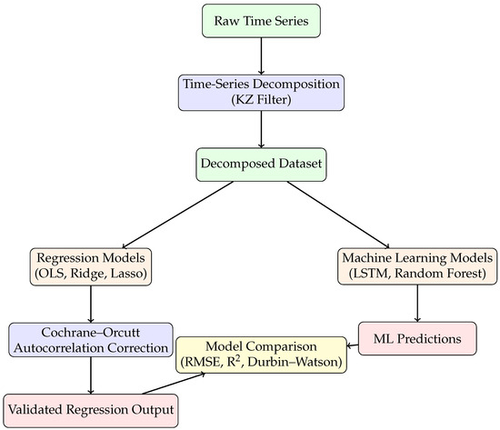
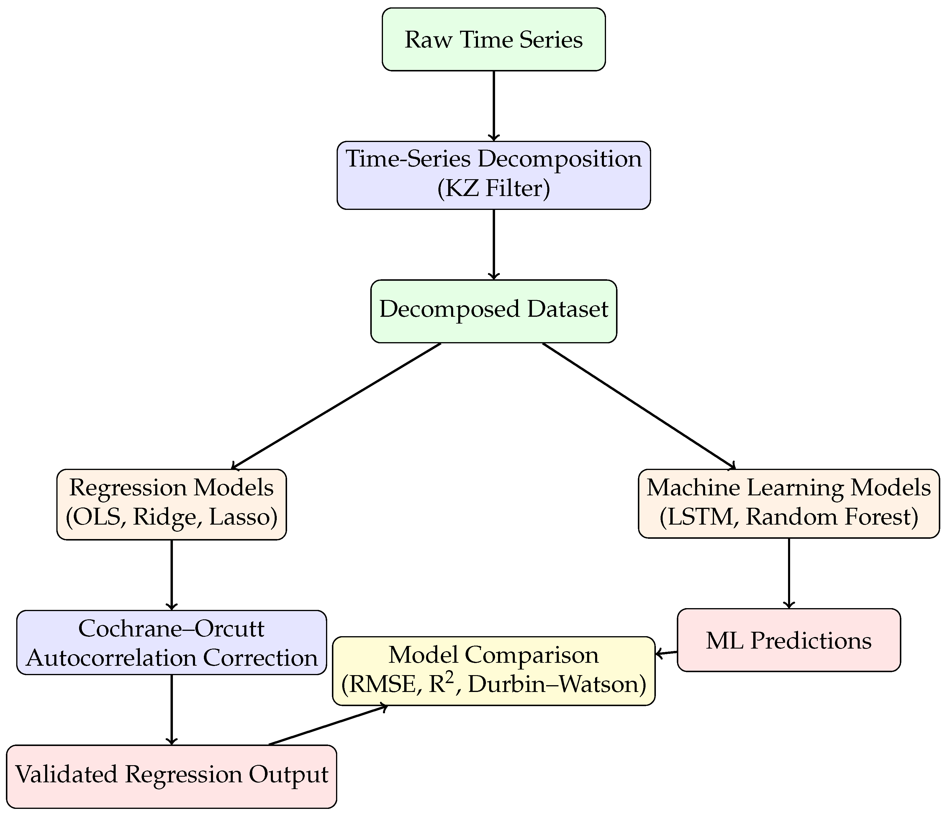
To improve the clarity and readability of the proposed methodology, Figure 1 summarizes the overall analytical framework adopted in this study. The flowchart illustrates the sequence of steps described in the following subsections, starting from the raw time series, followed by decomposition using the Kolmogorov–Zurbenko filter, and subsequent parallel modeling using regression-based and machine learning approaches. As shown in Figure 1, classical regression models are first estimated on the decomposed components, with autocorrelation addressed using the CO procedure. In parallel, machine learning models are trained using the same decomposed dataset. The outputs from both branches are finally evaluated and compared using standard performance and diagnostic metrics.

Figure 1. Framework for time-series decomposition using the Kolmogorov–Zurbenko filter, regression modeling with Cochrane–Orcutt correction, and machine learning approaches for temperature forecasting.

2.2. Study Data

This study is based on a daily time series collected at a single hydrological site from 1 January 2009 to 31 December 2020, comprising a total of 4383 observations. Model performance was evaluated using a walk-forward validation scheme, in which the first 2629 samples were used as the initial training set, followed by 1754 sequential one-step-ahead test steps. After each prediction, the training set was updated to include the most recently observed value, ensuring that the model was always trained on the latest available information before forecasting the next step. This approach mimics real-world operational forecasting, where new observations become available continuously, and allows the model to adapt over time. This walk-forward method provides a robust, realistic assessment of predictive performance under evolving temporal conditions. Although the dataset provides sufficient temporal coverage for model development and validation, its focus on a single location may limit the generalizability of the findings. Future studies could incorporate multiple sites or longer observational periods to assess the robustness of the proposed framework under diverse environmental conditions. Daily meteorological variables were obtained from NASA’s POWER data repository. These include incoming surface shortwave radiation under all-sky conditions (ALLSKY_SFC_SW_DWN, W/m²;), which represents the solar irradiance reaching the Earth’s surface; root-zone soil moisture (GWETROOT, fraction 0–1), representing water content in the top 1 m of soil derived from MERRA-2; wind speed at 2 meters (WS2M, m/s) describing near-surface horizontal wind; relative humidity at 2 meters (RH2M, %), representing the percentage of atmospheric moisture; and air temperature at 2 meters (T2M, °C), describing the near-surface thermal environment. These variables form the meteorological inputs used in model training. Hydrological variables were obtained from the United States Geological Survey (USGS). Daily streamflow at the Des Moines River gauge near Keosauqua (Logflow, m³/s, log-transformed) was used as the primary hydrological response variable. Additionally, groundwater levels from a monitoring well in Jefferson County (Groundwater Level, m) were included to capture subsurface hydrological dynamics. Combined, these meteorological and hydrological datasets provide a comprehensive set of inputs for the modeling framework.

2.3. Autocorrelation Treatment in Classical Regression and LSTM Models

In the classical regression framework, including OLS, Ridge, and Lasso models, autocorrelation in the residuals was addressed using the CO procedure. Assuming an AR(1) structure in the error term,

$${\epsilon }_t=\rho {\epsilon }_{t-1}+e_t,\left|\rho \right|<1,$$

(1)

the autocorrelation parameter $\rho$ is estimated iteratively until convergence. The regression model is then transformed as

$$y_t-\rho y_{t-1}=\alpha (1-\rho )+\beta (X_t-\rho X_{t-1})+e_t,$$

(2)

yielding coefficient estimates with reduced serial correlation and corrected standard errors. This explicit estimation of $\rho$ is a defining feature of classical econometric correction techniques, in which temporal dependence is specified and addressed directly. The applicability of the Cochrane–Orcutt procedure relies on several assumptions. First, the residual process is assumed to be stationary and adequately described by a first-order autoregressive structure. Second, the underlying regression model must be correctly specified and linear in parameters. Under these conditions, the transformation improves estimator efficiency and restores the validity of statistical inference. However, the method may be less effective when higher-order autocorrelation, structural breaks, or strong nonstationarity are present, and it reduces the effective sample size due to the loss of the initial observation. These limitations motivate the use of Cochrane–Orcutt primarily as a correction technique within classical linear regression models rather than as a general solution for complex nonlinear time-series data. In contrast, the machine learning approach based on Long Short-Term Memory (LSTM) networks does not impose a predetermined autocorrelation structure and does not require separate estimation of $\rho$. Temporal dependence is learned implicitly through the recurrent weight matrices and gating mechanisms of the LSTM. These recurrent parameters act analogously to the AR(1) coefficient by regulating the flow of information from time step $t-1$ to t. During training, backpropagation jointly optimizes these temporal weights along with all other network parameters and hyperparameters. As a result, the LSTM is capable of capturing both linear and nonlinear autocorrelation patterns without the need for iterative correction procedures such as Cochrane–Orcutt or the explicit specification of an AR(1) model. Consequently, autocorrelation treatment in this study follows a model-specific strategy: explicit residual correction via Cochrane–Orcutt for classical regression models, and implicit temporal learning through recurrent dynamics for LSTM-based models.

2.4. Kolmogorov–Zurbenko (KZ) Filtering, Spectral Characteristics, and Decomposition of the T2M Temperature Series

The Kolmogorov–Zurbenko (KZ) filter is a nonparametric, iterative moving-average technique that smooths autocorrelated time series, effectively separating long-term trends from short-term fluctuations [7]. It has been extensively applied across various scientific domains for its robust ability to separate time series into distinct spectral components. The foundational work by [21] established the theoretical basis for analyzing non-stationary processes. In climate science, the KZ filter has been validated for isolating long-term stratospheric dynamics, while in environmental monitoring, it has been used successfully to disentangle temporal patterns of traffic-related air pollutants [22,23].

Furthermore, the KZ filter has been applied in hydrological studies [24] to decompose multivariate water discharge data and improve forecasting accuracy. Its versatility is further illustrated in air quality research, including quantification of long-term meteorological and emission impacts [25], predictive modeling of ozone concentrations via KZ–LSTM hybrid approaches [26], and dynamic evaluation of regional air quality models [27]. Collectively, these applications demonstrate the filter’s capacity to provide physically interpretable decompositions of complex time series across different fields.

The KZ filter’s formulation allows interpretation in both the time and frequency domains, making it particularly well suited to climate and environmental datasets characterized by strong seasonality, long-term variability, and synoptic-scale noise [28,29].

In the time domain, the KZ filter applies repeated centered moving averages of window length m (odd integer) to the original series $X_t$, such that

$$\mathrm{KZ}[X_t;m,k]=\underset{k\mathrm{iterations}}{\underbrace{M_m\left(M_m(\dots M_m\left(X_t\right))\right)}},$$

(3)

where

$$M_m\left(X_t\right)={\displaystyle \frac{1}{m}}\sum _{j=-{\displaystyle \frac{m-1}{2}}}^{{\displaystyle \frac{m-1}{2}}}{X}_{t+j}.$$

(4)

Larger values of m widen the smoothing window, while higher k produce progressively stronger attenuation of high-frequency fluctuations. In the frequency domain, the KZ filter behaves as a tunable low-pass filter with transfer function

$$H(f;m,k)={\left[{\displaystyle \frac{sin\left(\pi mf\right)}{msin\left(\pi f\right)}}\right]}^{2k},$$

(5)

which leads to exponential suppression of high-frequency energy and strong preservation of low-frequency climate signals. This dual-domain structure offers flexible control of both temporal and spectral smoothing, providing an effective intermediate between simple moving averages and strict spectral filters [30,31].

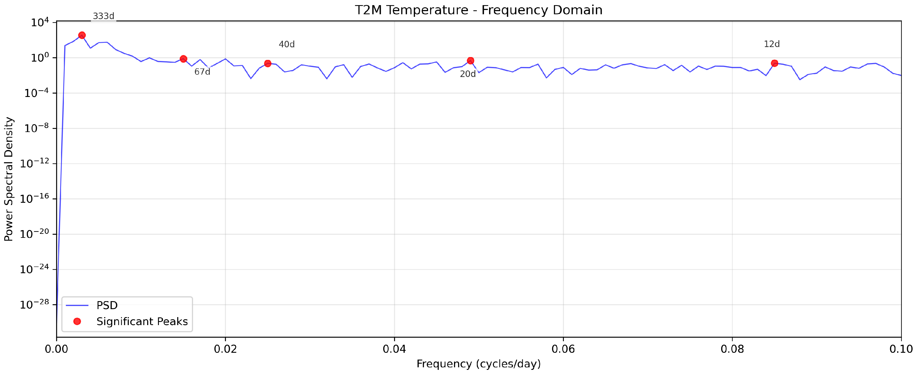
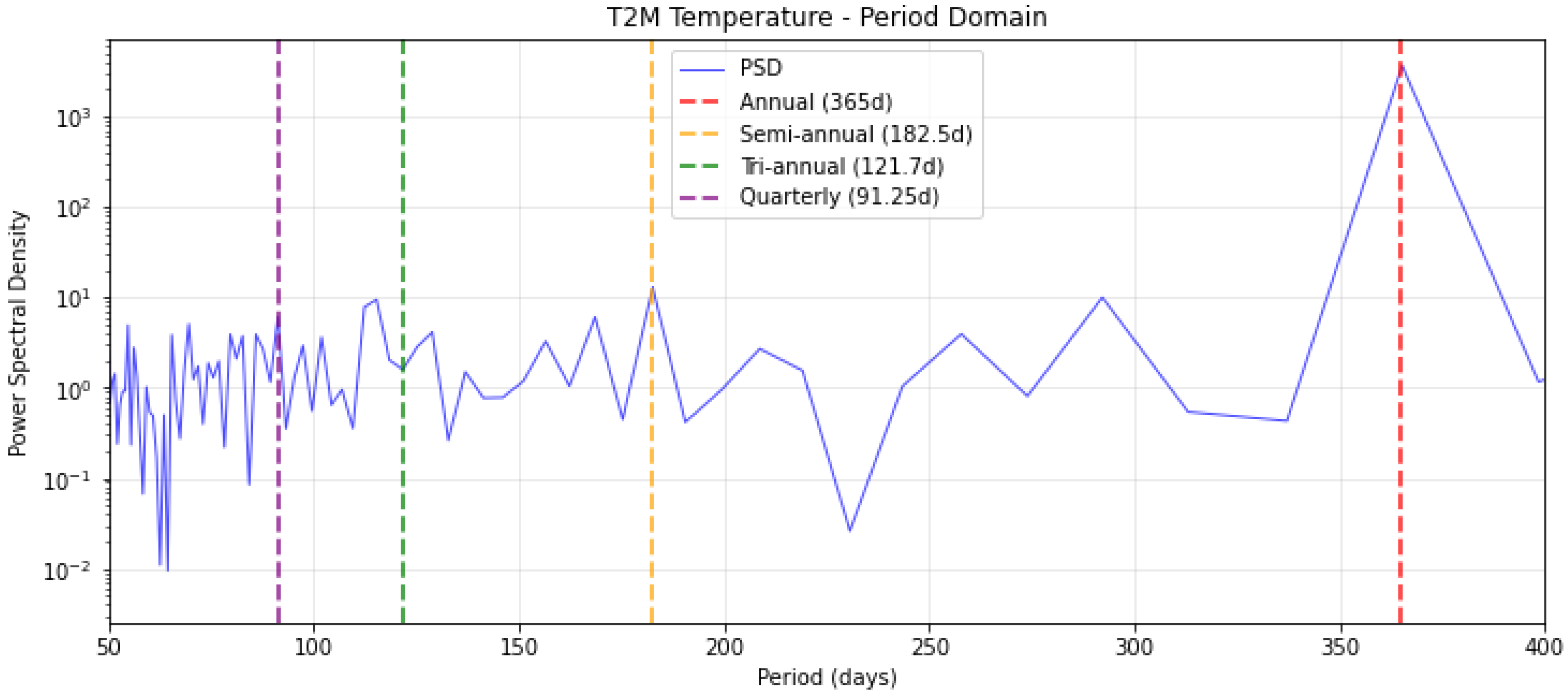
To identify the intrinsic periodicities of the standardized T2M temperature series and guide the selection of filter parameters, frequency-domain characteristics were examined using the power spectral density (PSD). Figure 2 and Figure 3 display the resulting periodogram of the T2M series, revealing a multi-scale structure characteristic of climatic temperature signals. A dominant peak at $f=0.0021$ cycles/day corresponds to the annual (365-day) cycle, accompanied by harmonics at integer multiples ($2f$, $3f$, $4f$), indicating a non-sinusoidal seasonal profile. The monotonic red-noise slope at higher frequencies is consistent with climate systems governed by low-frequency forcing. The period-domain representation reveals physically meaningful scales, including the semi-annual (182.5-day), seasonal (121.7-day), and quarterly (91.25-day) components.

Figure 2. Power spectral density of T2M temperature in the frequency domain, indicating dominant harmonic cycles.

Figure 3. Period-domain power spectrum of T2M temperature illustrating dominant physical timescales.

Based on this spectral evidence, the filter configuration ${\mathrm{KZ}}_{365,3}$ was selected to isolate long-term climate variability from seasonal and short-term processes. Applying ${\mathrm{KZ}}_{365,3}$ yields a three-component decomposition of the T2M series. The long-term component captures smooth interannual variations free from seasonal or synoptic fluctuations, representing large-scale climate processes. The seasonal component reconstructs the annual cycle with clear amplitude modulation and preserved harmonic structure. The short-term component resembles white or weakly correlated noise, containing weather-scale fluctuations lacking persistent periodic structure.

The spectral correspondence of these components is summarized in Table 1. Frequencies below 0.0021 cycles/day define the long-term band (explaining 0.62% of variance), the range 0.0021–0.005 cycles/day corresponds to the seasonal component (81.85%), and frequencies above 0.005 cycles/day represent short-term variability (12.06%). These percentages were obtained by integrating the spectral density $S\left(f\right)$ over each band:

$${\sigma }_{\mathrm{long}}^2={\int }_0^{0.0021}S\left(f\right)df$$

(6)

$${\sigma }_{\mathrm{seasonal}}^2={\int }_{0.0021}^{0.005}S\left(f\right)df$$

(7)

$${\sigma }_{\mathrm{short}}^2={\int }_{0.005}^{f_{\mathrm{nyquist}}}S\left(f\right)df,$$

(8)

and normalizing by the total variance. This technique for variance decomposition is a standard practice in spectral analysis [32,33], with deep roots in climatology where it is used to separate distinct physical processes based on their characteristic timescales [34,35]. This decomposition provides a physically interpretable separation of climate-scale, seasonal, and synoptic components, validating the KZ_365,3 configuration for the analysis of climatic time series.

Table 1. Spectral decomposition of time series components. Frequency units are in cycles per day (cpd).

Component	Frequency (cpd)	Variance	Interpretation
Long-term	<0.0021	0.62%	Climate trends
Seasonal	$0.0021$–$0.005$	81.85%	Annual cycle
Short-term	>0.005	12.06%	Weather noise

3. Results

This work focuses on autocorrelation as the central challenge in near-surface air temperature (T2M) time-series forecasting, and systematically evaluates model performance under integrated data treatments. The analysis combines raw and Kolmogorov–Zurbenko (KZ)-decomposed data, with and without explicit autocorrelation correction, within a unified experimental framework. This design enables a direct and transparent comparison of alternative autocorrelation management strategies across both classical regression models and machine learning approaches. The section is organized into two parts: (i) Analysis of Raw and Decomposed Data Using Classical Methods and (ii) Analysis of Raw and Decomposed Data Using Machine Learning Methods. All models are evaluated using an expanding-window walk-forward validation scheme with one-step-ahead forecasting. An initial subset of the time series is used for model training, after which forecasts are generated sequentially for each subsequent time step. At each iteration, the model is trained using all observations available up to the previous time point and is then used to predict the next observation. Once the true value becomes available, it is incorporated into the training set, and the procedure is repeated. This protocol closely mimics real-time operational forecasting and ensures that no future information is used at the time of prediction. For the linear regression models (OLS, Ridge, and Lasso), autocorrelation is explicitly addressed using the CO procedure. At each walk-forward step, the model is fitted on the current training window, residuals are computed, and the AR(1) coefficient $\rho$ is estimated from these residuals. The estimated $\rho$ is then used to transform both the predictors and the response prior to refitting the model. As the training set expands over the walk-forward iterations, $\rho$ is re-estimated at each step and therefore evolves over time, while remaining constant within each individual model fit. In contrast, for the LSTM model, $\rho$ is introduced as a trainable parameter and is jointly optimized with the network weights via gradient-based learning. This allows autocorrelation to be modeled directly within the nonlinear learning process, rather than through residual-based post-processing. For all models, diagnostic statistics such as the Durbin–Watson test are computed post hoc on forecast residuals and are used solely to assess remaining autocorrelation; they are not involved in the estimation of $\rho$.

3.1. Classical Regression Analysis with and Without the Cochrane–Orcutt Correction

Recent studies have demonstrated that hybrid decomposition–regression–AI frameworks significantly improve runoff prediction in nonlinear and non-stationary environments [8]. These findings support the present study’s strategy of modeling decomposed components separately using regression and machine learning techniques. The study employs two parallel analytical pathways: one based on raw data and another based on decomposition-derived predictors. In the raw-data pathway, regression models are evaluated both with and without the CO transformation to quantify the effect of explicit autocorrelation correction. In the decomposed-data pathway, the target variable is modeled using a unified set of predictors constructed from the long-term, seasonal, and short-term components obtained through the KZ filter. These component variables jointly serve as explanatory inputs in a single regression formulation rather than being modeled separately. The two analytical streams are then integrated into a unified comparative framework that evaluates OLS, Ridge, and Lasso across all data-treatment conditions. This structure clarifies the interaction between explicit CO correction and decomposition-based pre-processing. It also tests whether decomposition offers benefits beyond applying autocorrelation correction to the raw series.

In Table 2, the regression results for both the raw and KZ-filtered temperature series show a clear contrast in how autocorrelation and predictive accuracy are managed. For the raw data, all models exhibit strong positive autocorrelation prior to correction, with Durbin–Watson values close to 0.90, accompanied by modest explanatory power ($R^2\approx 0.61$–0.62) and relatively high prediction error (RMSE = 0.62). Applying the Cochrane–Orcutt procedure improves these models by reducing serial correlation and increasing the Durbin–Watson statistic to around 1.47–1.50, while also lowering the RMSE to 0.51 and raising $R^2$ to approximately 0.73–0.74. In contrast, the KZ-filtered data provide a substantially stronger baseline: even before applying Cochrane–Orcutt, the models achieve Durbin–Watson values around 1.06–1.08, with lower RMSE (0.37) and considerably higher $R^2$ (0.86). When Cochrane–Orcutt is applied to the KZ-filtered series, the Durbin–Watson statistic approaches the ideal value of 2.0, indicating that residual autocorrelation is effectively removed; this correction yields further, though modest, gains in RMSE (0.32–0.33) and $R^2$ (0.89). Overall, the results show that while Cochrane–Orcutt enhances the performance of the raw-data models, the KZ decomposition plays the more central role by restructuring the series in a way that substantially reduces autocorrelation and improves predictive behavior even before correction, with the combination of KZ filtering and Cochrane–Orcutt producing the most stable and accurate models.

Table 2. Model Performance: Raw vs. KZ-Filtered Data.

Raw Data				KZ-Filtered Data
Model	RMSE	R2	DW	Model	RMSE	R2	DW
OLS	0.62	0.61	0.90	COMB-OLS	0.37	0.86	1.08
OLS-CO	0.51	0.73	1.47	COMB-OLS-CO	0.32	0.89	1.99
Ridge	0.62	0.61	0.90	COMB-Ridge	0.37	0.86	1.08
Ridge-CO	0.51	0.73	1.47	COMB-Ridge-CO	0.32	0.89	2.00
Lasso	0.62	0.62	0.91	COMB-Lasso	0.37	0.86	1.06
Lasso-CO	0.51	0.74	1.50	COMB-Lasso-CO	0.33	0.89	2.02

Table 3 presents the estimated coefficients obtained from the OLS, Ridge, and Lasso regression models for the raw data. The results show that ALLSKY_SFC_SW_DWN (shortwave solar radiation) has the strongest positive influence on the dependent variable (coefficient $\approx 0.64$), followed by PRECTOTCORR (precipitation) and RH2M (relative humidity). In contrast, GWETROOT (root-zone soil moisture) and GROUNDWATER exhibit negative relationships, suggesting that higher soil and groundwater moisture are associated with lower predicted values. The coefficients are largely consistent across the three models, indicating model robustness and limited multicollinearity. These findings align with the model performance metrics discussed earlier, where all models demonstrated improved accuracy and reduced autocorrelation after correction using the Cochrane–Orcutt method.

Table 3. Coefficients of the Raw Data Model and Regularization Methods.

Predictor	OLS_coef	Ridge_coef	Lasso_coef
ALLSKY_SFC_SW_DWN	0.64	0.64	0.63
GROUNDWATER	−0.23	−0.23	−0.21
GWETROOT	−0.60	−0.60	−0.55
LOGFLOW	0.22	0.22	0.21
PRECTOTCORR	0.26	0.26	0.26
RH2M	0.25	0.25	0.21
WS2M	−0.06	−0.06	−0.07

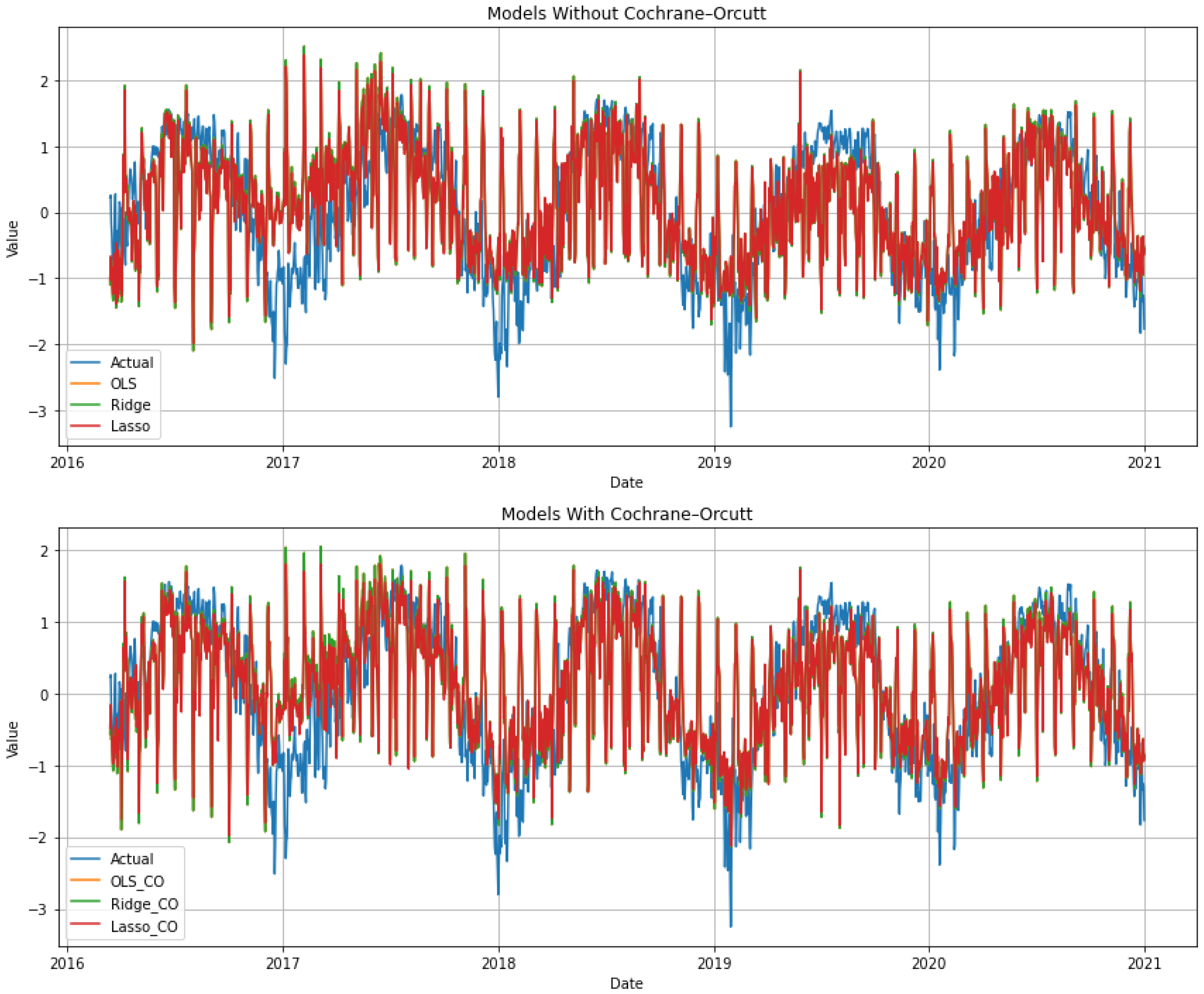
Figure 4 shows that the classical regression models applied to the raw data produce visibly noisier predictions and greater divergence from the observed values, indicating the presence of strong autocorrelation. After applying the CO correction, the fitted series align much more closely with the actual data, and the temporal fluctuations become smoother. This visual comparison confirms the statistical improvements observed in the analysis, demonstrating that autocorrelation correction substantially enhances model fidelity and predictive stability.

Figure 4. Classic model predictions on raw data, comparing results with and without Cochrane–Orcutt correction.

To complement these results, the coefficients of the combined KZ-based temperature model are presented in Table 4. Each regression method (OLS, Ridge, and Lasso) produces a single integrated model, and the table lists its coefficients across the three temporal structures. The first group of columns corresponds to the long-term coefficients, the second group to the seasonal coefficients, and the third group to the short-term coefficients. Thus, the final temperature estimate is determined by the sum of a predictor’s effects across all three components. For the combined OLS model, the long-term coefficients indicate that ALLSKY_SFC_SW_DWN (1.88) and GWETROOT (0.46) contribute strongly to the underlying temperature trend, while PRECTOTCORR shows a pronounced negative long-term influence ($-3.08$). In the seasonal part of the model, ALLSKY_SFC_SW_DWN remains influential (0.54), contributing to the strength of the seasonal cycle. The short-term coefficients are smaller in magnitude, with RH2M (0.26) and ALLSKY_SFC_SW_DWN (0.18) contributing to higher-frequency temperature fluctuations.

Table 4. Coefficients of the Combined Model and Regularization Methods.

Predictor	Long-Term			Seasonal			Short-Term
	OLS	Ridge	Lasso	OLS	Ridge	Lasso	OLS	Ridge	Lasso
ALLSKY_SFC_SW_DWN	1.88	0.07	0.04	0.54	0.40	0.42	0.18	0.11	0.08
WS2M	−0.06	0.00	−0.01	−0.74	−0.31	−0.32	0.06	0.05	0.04
RH2M	−0.09	−0.03	0.00	−0.24	−0.12	−0.12	0.26	0.19	0.16
PRECTOTCORR	−3.08	−0.22	−0.02	0.68	0.17	0.15	0.03	0.03	0.01
LOGFLOW	0.10	0.05	0.01	0.16	0.11	0.09	0.12	0.04	0.02
GROUNDWATER	0.11	0.07	0.00	−0.02	−0.01	0.00	−0.21	−0.03	−0.01
GWETROOT	0.46	0.27	0.00	−0.20	−0.12	−0.09	−0.45	−0.08	−0.05

The Ridge model preserves the overall structure of the OLS solution but shrinks the magnitudes toward zero, producing more stable long-term and seasonal coefficients while maintaining the same directional relationships. The short-term effects are also reduced but remain consistent with the underlying variability patterns. The Lasso model applies more stringent regularization, driving some of the smaller coefficients to exactly zero and retaining only the most influential predictors in each temporal component. Radiation (ALLSKY_SFC_SW_DWN) remains important across all components, while variables such as WS2M and GWETROOT appear only where their contribution is substantial.

Overall, the table highlights how each regression method constructs a unified temperature model by combining long-term, seasonal, and short-term structures derived from the KZ filter. The coefficients reveal the relative importance of each predictor at different temporal scales, with radiation exerting consistent influence, precipitation shaping the long-term baseline, and humidity and soil moisture affecting short-term fluctuations. Regularization through Ridge and Lasso enhances stability and sparsity while preserving the key relationships captured by the combined model.

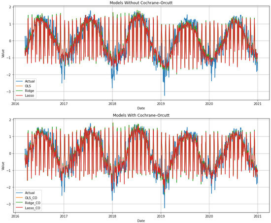
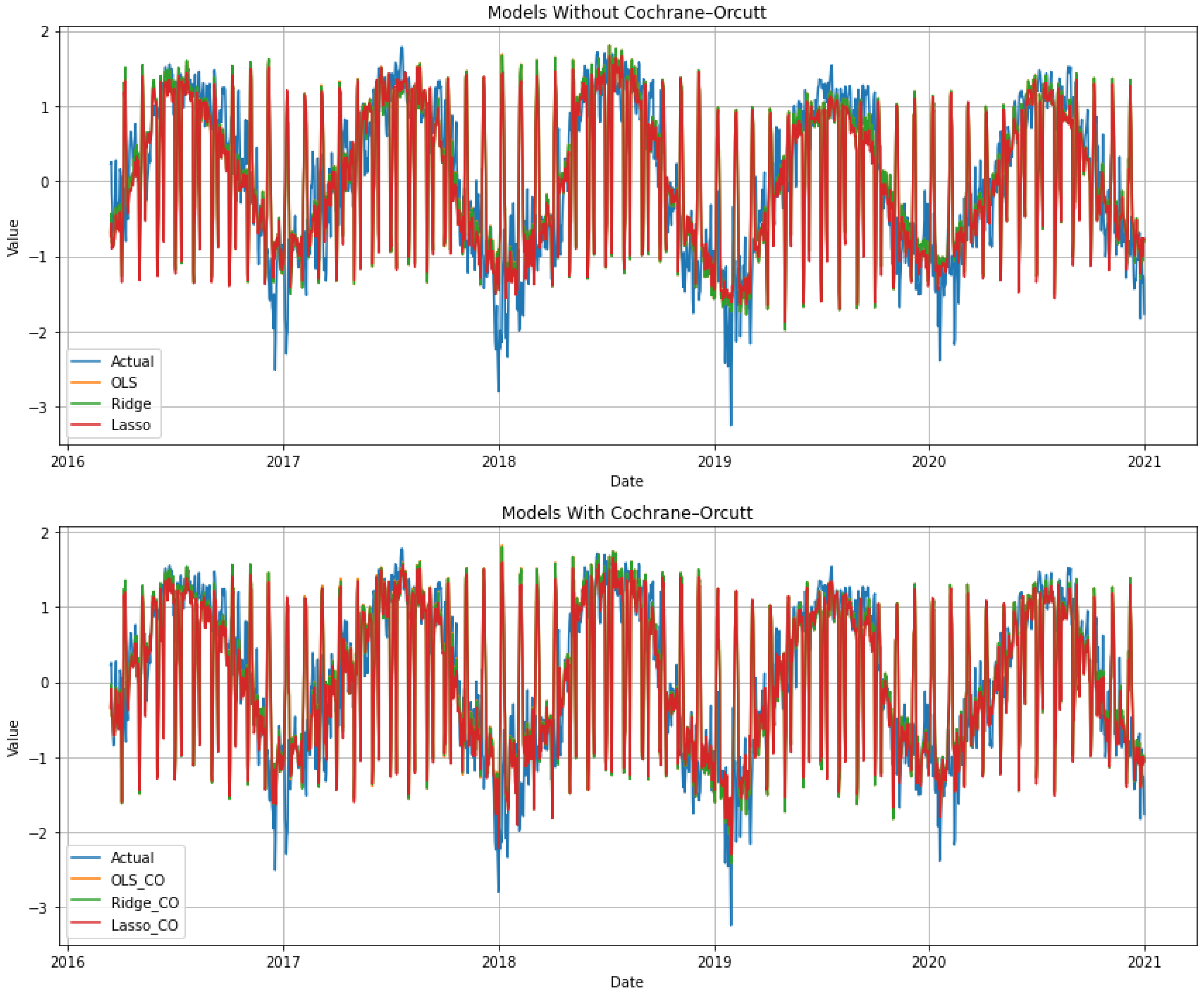
Figure 5 compares the combined predictions derived from the decomposed data with and without the CO adjustment. The results show that applying the correction improves the alignment with the actual series, producing smoother reconstructed values and reducing the residual autocorrelation effects that are still present in the uncorrected models.

Figure 5. Combined model predictions on decomposed data, comparing results with and without Cochrane–Orcutt correction.

3.2. Machine Learning Analysis Using LSTM Models with and Without the Autocorrelation Coefficient ($\rho$)

While neural networks have gained popularity for time series forecasting, they typically do not explicitly account for autocorrelated errors—a challenge that classical econometrics has long addressed for linear models [20]. The CO procedure, for instance, is specifically designed for linear regression and cannot be directly applied to nonlinear LSTM models. In LSTMs, temporal dependence is instead handled through sequential learning and the incorporation of an autocorrelation coefficient ($\rho$). To address this limitation, Sun et al. (2021) proposed a method to jointly estimate the autocorrelation coefficient alongside model parameters using gradient descent [20]. Long Short-Term Memory (LSTM) networks address autocorrelation through architectural rather than statistical mechanisms, relying on recurrent connections and memory cells to internalize temporal dependencies. In this study, LSTM performance is evaluated using both raw data and decomposition-derived predictors to determine the network’s capacity to manage serial correlation without explicit correction procedures. Application to raw data assesses whether the LSTM architecture can transform autocorrelation into useful predictive structure directly from the integrated series. In parallel, LSTM modeling with decomposed inputs—where trend, seasonal, and residual components are supplied as separate predictors—examines whether structured decomposition enhances the network’s ability to learn distinct temporal patterns. Together, these analyses provide a comparative assessment of whether neural network architectures inherently mitigate autocorrelation or benefit further from pre-processing strategies that isolate key temporal dynamics. The LSTM model consists of two LSTM layers with 64 and 32 hidden units, respectively, followed by dropout layers with rates of 0.3 and 0.2, and dense layers with 16 and 1 units. The selection of LSTM hyperparameters was guided by prior studies in environmental and hydrological time-series forecasting [7,16,19], as well as iterative experimentation to balance model complexity and generalization. Specifically, the sequence length was set to 10, the learning rate to 0.0005, the batch size to 32, and training was performed with 5 initial epochs followed by 1 epoch per walk-forward step. These hyperparameters were chosen to ensure stable convergence and to prevent overfitting while capturing multi-scale temporal dependencies. The model was then trained jointly with the autocorrelation coefficient $\rho$ using the walk-forward approach. In the LSTM model, the autocorrelation parameter $\rho$ is treated as a trainable variable, initialized as an unconstrained scalar ${\rho }_{\mathrm{raw}}$ and transformed via the hyperbolic tangent function to enforce the stationarity constraint $\left|\rho \right|<1$. The joint optimization of $\rho$ and the LSTM network weights is performed using the Adam optimizer with a learning rate of 0.0005. During training, convergence is monitored by tracking the mean squared error (MSE) loss on the training data and the evolution of $\rho$ across epochs. Additionally, in the walk-forward evaluation, $\rho$ is updated online at each step to reflect the most recent temporal dependencies. The final learned value of $\rho$ is reported to ensure reproducibility and to demonstrate stable convergence, providing a statistically rational treatment of autocorrelation in the LSTM framework.

3.2.1. LSTM Analysis Without Autocorrelation Coefficient ($\rho )$

Table 5 shows that using KZ-filtered data provides a modest improvement in LSTM performance compared to using raw data, even before incorporating the autocorrelation coefficient $\rho$. Specifically, the $R^2$ score increases from 0.60 for the raw data to 0.62 for the KZ-filtered data, suggesting that the decomposition captures additional variance that enhances the model’s explanatory power. Correspondingly, the RMSE decreases from 0.62 to 0.60, indicating a modest reduction in prediction error and improved overall fit. The Durbin–Watson statistic decreases from 1.56 in the raw data to 1.41 in the KZ-filtered data, implying that the autocorrelation of residuals is slightly more pronounced in the decomposed data. While values closer to 2 indicate no autocorrelation, this small reduction does not appear to substantially undermine model reliability but suggests that serial correlation is still present and could be considered in subsequent modeling or residual diagnostics. It should be noted that these results were obtained using identical LSTM hyperparameters for both the raw and decomposed datasets. Maintaining consistent hyperparameter settings ensures that the observed differences in performance are attributable primarily to the data decomposition rather than changes in model configuration. Overall, the application of the KZ filter and use of decomposed components provide a small but consistent improvement in LSTM predictive performance, enhancing variance explanation and prediction accuracy while moderately affecting residual autocorrelation.

Table 5. LSTM Walk-Forward analysis without autocorrelation coefficient.

Raw Data				KZ-Filtered Data
Metric	RMSE	R2	DW	Metric	RMSE	R2	DW
Values	0.62	0.60	1.56	Values	0.60	0.62	1.41

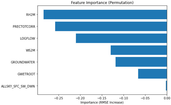
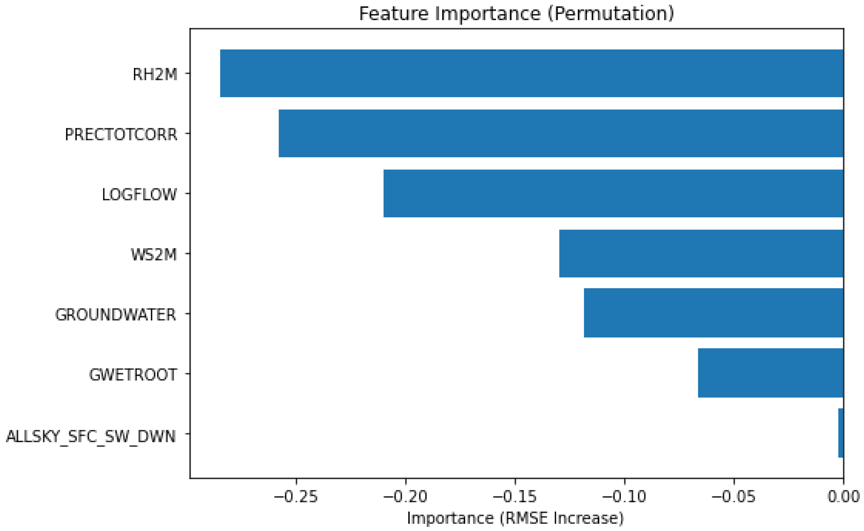
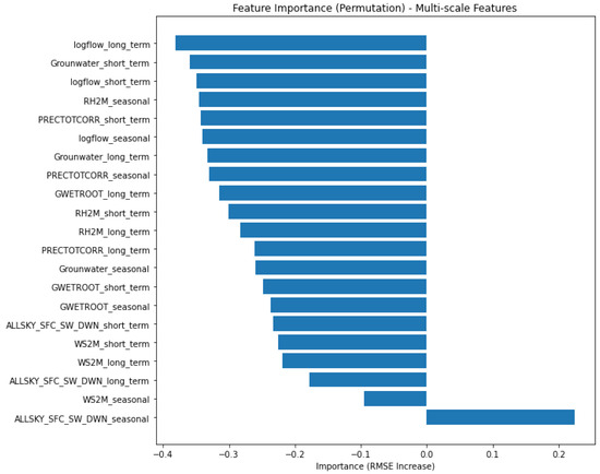
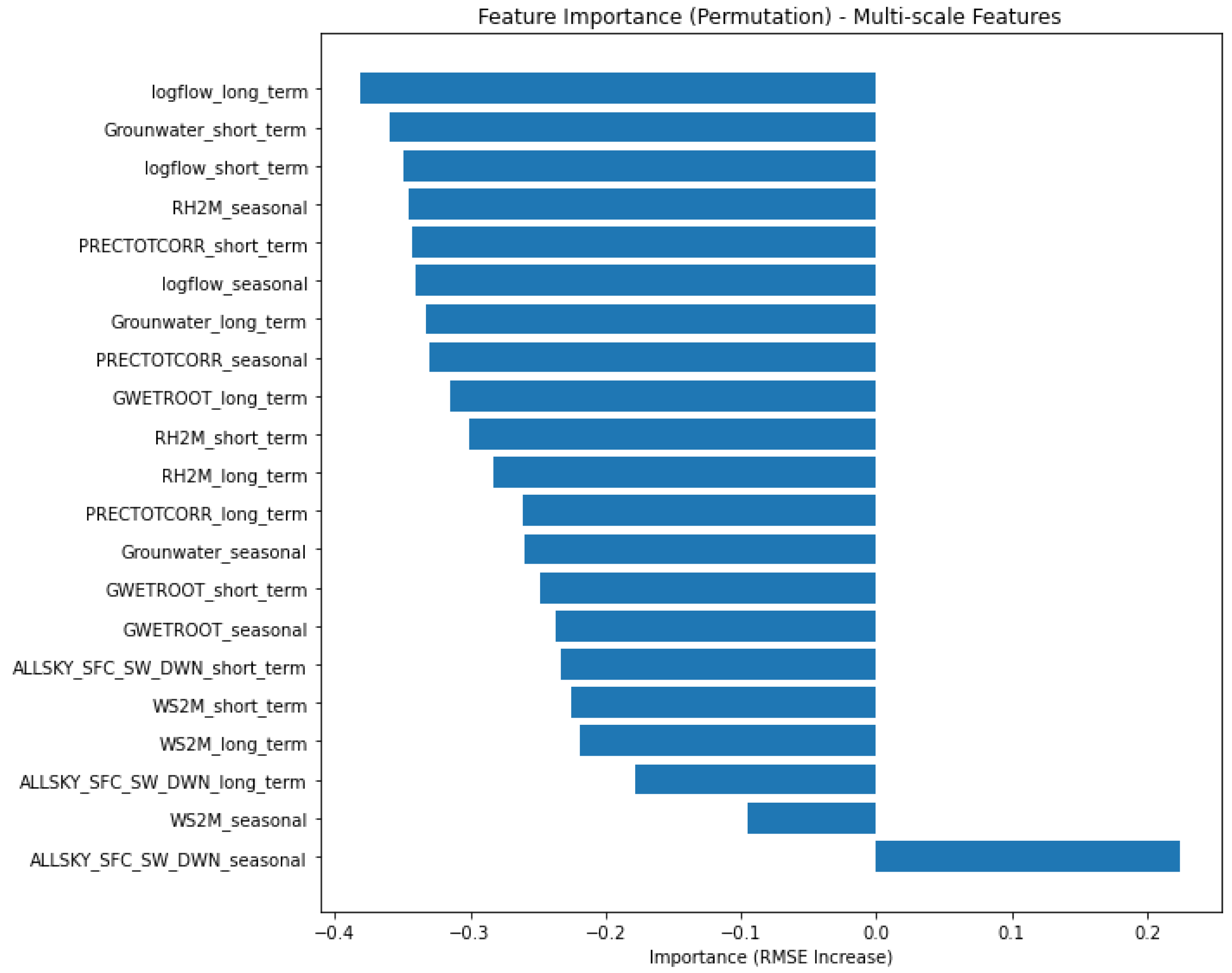
The comparison between the raw-feature model and the KZ-decomposed multi-scale model shows a clear difference in how the LSTM assigns importance to predictors. The permutation importance results in Figure 6 show that RH2M is the most influential predictor in the raw-data LSTM model, producing the largest increase in RMSE when permuted. It is followed by PRECTOTCORR and LOGFLOW, both of which exhibit strong positive contributions to prediction accuracy. WS2M and GROUNDWATER also provide meaningful influence, though with smaller magnitudes. In contrast, GWETROOT and ALLSKY_SFC_SW_DWN have minimal effect on model performance, indicating that the raw model is relatively insensitive to these variables. Overall, the model relies heavily on a small subset of predictors, with moisture, precipitation, and long-term flow information contributing most to its predictive skill. In contrast, as shown in Figure 7, the KZ-decomposed model exhibits a much richer and more distributed importance pattern. The highest importance is assigned to logflow_long_term, highlighting the dominant predictive role of long-term variability in streamflow. Many other long-term, seasonal, and short-term components also appear influential, showing that the LSTM draws predictive information from specific temporal scales rather than from the raw variables alone. Short-term components such as groundwater_short_term and PRECTOTCORR_short_term are important, emphasizing the strong role of high-frequency variability. Seasonal components including RH2M_seasonal and GWETROOT_seasonal also contribute substantially, while several long-term components such as GWETROOT_long_term and RH2M_long_term show moderate importance. Overall, the results demonstrate that the raw-feature model captures only broad aggregated relationships, whereas the decomposed model uncovers detailed multi-scale dependencies. This confirms that KZ decomposition enhances the LSTM’s ability to detect meaningful temporal patterns that remain hidden when using non-decomposed predictors. Overall, the prominence of decomposed components—particularly long-term and short-term signals—indicates that the LSTM benefits from the separation of temporal dynamics, enabling it to learn distinct patterns associated with sustained trends, cyclical behavior, and rapid fluctuations that are less evident when using raw variables alone.

Figure 6. Feature importance of predictors for the raw-data LSTM model.

Figure 7. LSTM feature importance for KZ–decomposed predictors.

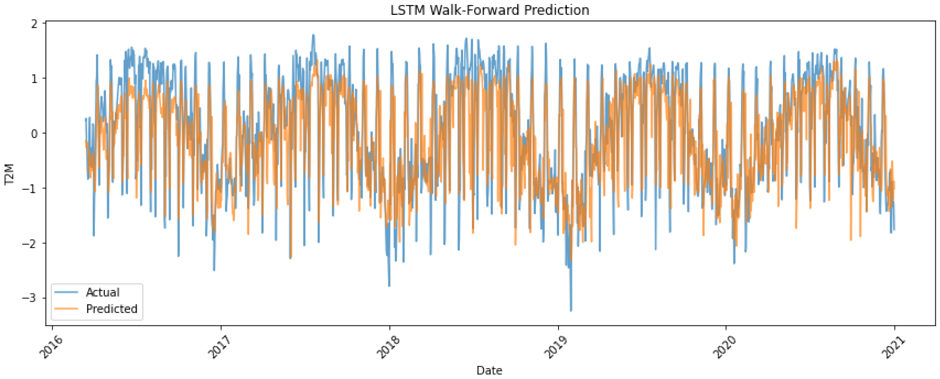
Figure 8 shows that the LSTM trained on raw data follows the general signal but with larger deviations. In contrast, Figure 9 demonstrates that the KZ-decomposed inputs produce predictions that more closely track the observed dynamics, indicating improved stability and alignment.

Figure 8. LSTM predictions using raw data.

Figure 9. LSTM predictions using KZ-decomposed data.

3.2.2. LSTM Analysis with Autocorrelation Coefficient ($\rho )$

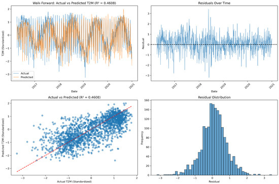
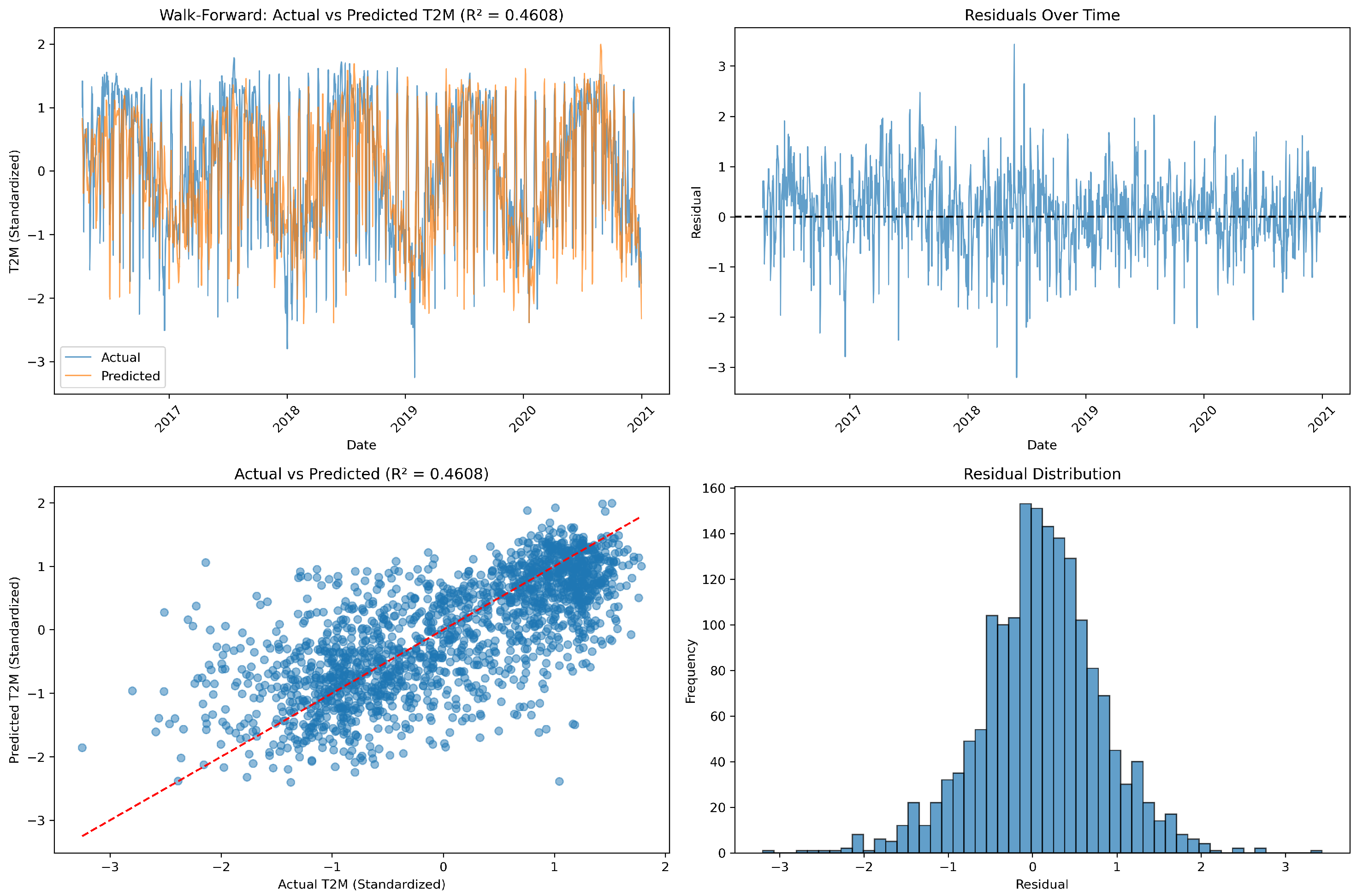
The results in Table 6 show that integrating the KZ filter with the autocorrelation-adjusted LSTM substantially improves forecasting performance. Using raw data, the model attains moderate accuracy (RMSE = 0.73, $R^2=0.46$) and exhibits strong positive residual autocorrelation (DW = 0.79), indicating that short-term noise limits the network’s ability to learn stable temporal patterns even with the learned correction parameter $\rho$. In contrast, applying the KZ filter produces a smoother and more structured input signal, leading to improved accuracy (RMSE = 0.59, $R^2=0.63$) and residuals that are nearly uncorrelated (DW = 1.84). These findings demonstrate that KZ pre-processing enhances the effectiveness of the autocorrelation-adjusted LSTM by reducing noise, improving learnability, and yielding statistically valid residual behavior. Table 5 and Table 6 present the complete set of LSTM configurations considered in this study, comprising raw and KZ-filtered inputs with and without the autocorrelation coefficient ($\rho$). CO-based correction is not applied to LSTM models.

Table 6. LSTM Walk-Forward analysis with autocorrelation coefficient.

Raw Data				KZ-Filtered Data
Metric	RMSE	R2	DW	Metric	RMSE	R2	DW
Values	0.73	0.46	0.79	Values	0.59	0.63	1.84

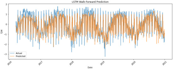
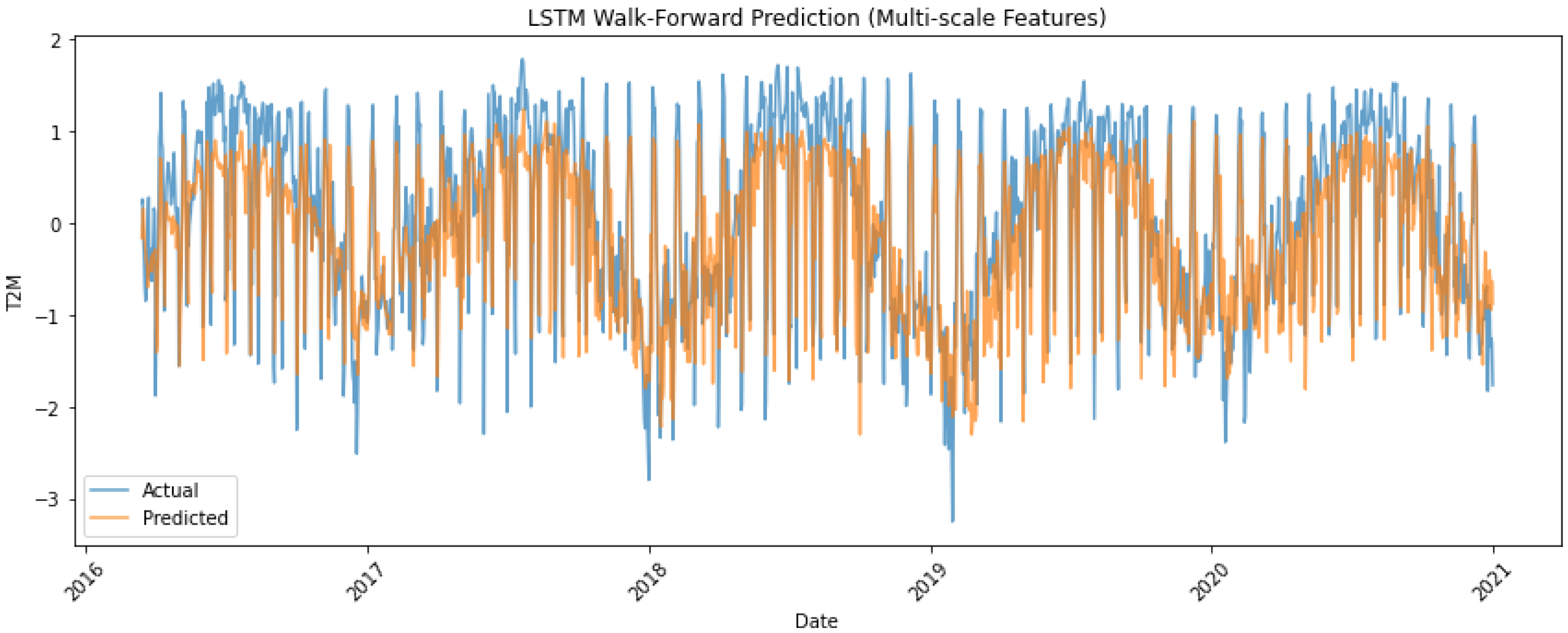
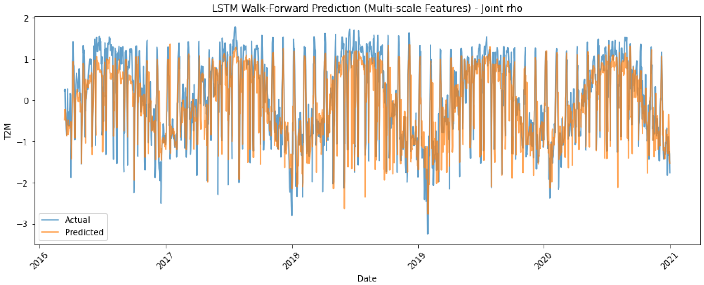
Figure 10 and Figure 11 compare the behavior of LSTM models trained on different predictor sets with embedded autocorrelation coefficient ($\rho$). Figure 10 shows the model trained on raw predictors, which successfully captures the dominant temporal dynamics of the series; however, noticeable local deviations, phase shifts, and heavy-tailed residuals indicate that unresolved noise and multi-scale dependence persist in the raw data. Although the learned $\rho$ reduces serial correlation, the Durbin–Watson statistic and residual diagnostics confirm that substantial autocorrelation remains. In contrast, Figure 11 demonstrates the KZ-filtered model, which exhibits markedly improved temporal coherence, with the predictions closely following the seasonal and intermediate-scale variations of the actual T2M series. The smoother KZ predictors enhance the signal-to-noise ratio, enabling the autocorrelation-adjusted LSTM to learn the underlying structure more effectively. As a result, the KZ-based model produces tighter predicted-versus-actual alignment, near-white residuals, and higher predictive accuracy, demonstrating that KZ decomposition and the embedded $\rho$ parameter work synergistically to stabilize the model and substantially reduce remaining autocorrelation.

Figure 10. LSTM predictions using raw data with $\rho$.

Figure 11. LSTM predictions using KZ-decomposed data with $\rho$.

4. Comparison and Conclusions

This study investigated the performance of classical time-series regression methods and modern neural sequence models for the prediction of surface air temperature, with particular emphasis on the treatment of autocorrelated errors and the role of multi-scale temporal decomposition. Across all experiments, the results clearly show that forecasting accuracy and statistical validity depend critically on handling both the multi-scale structure of environmental variables and the serial dependence inherent in meteorological time series.

Classical regression models demonstrated substantial improvements when paired with KZ decomposition and autocorrelation correction using the Cochrane–Orcutt procedure. Raw-data regressions exhibited strong residual autocorrelation and inflated significance levels, but the combination of temporal filtering and autoregressive error adjustment produced statistically valid models with high goodness-of-fit. This confirms that even linear models can achieve excellent performance when the dominant temporal components are separated and short-term noise is suppressed.

Neural methods showed analogous patterns. The LSTM trained on raw predictors with an embedded autocorrelation coefficient ($\rho$) captured major seasonal and interannual variations but retained noticeable residual autocorrelation and systematic local deviations. In contrast, when trained on KZ-filtered predictors, the same LSTM architecture exhibited markedly stronger predictive performance, higher $R^2$, lower RMSE, and residuals that were nearly white, as confirmed by the Durbin–Watson statistic. The network’s ability to jointly learn nonlinear dependencies and the autocorrelation parameter was effective only once the noisy, high-frequency components were removed through filtering. This finding parallels the classical results and underscores the importance of multi-scale pre-processing even for highly flexible learning architectures.

When comparing classical and neural approaches, the results highlight a consistent pattern: proper treatment of temporal dependence and scale separation has a greater impact on performance than model complexity. The best-performing classical models—after correcting for autocorrelation and incorporating filtered predictors—matched or exceeded the accuracy of the LSTM models in several configurations while preserving full interpretability. Neural models showed strengths in capturing nonlinear relationships and subtle predictor interactions, yet their performance depended on the same pre-processing steps and autocorrelation adjustments that enhanced the classical methods.

A key contribution of this work lies in the integrated nature of the proposed framework. Rather than relying on a single modeling paradigm, the analysis combines multi-scale decomposition, explicit autocorrelation correction, and walk-forward evaluation within a unified design. This allows each method to operate on signals with reduced temporal confounding while preserving statistical validity and operational realism. The results demonstrate that when temporal structure is explicitly addressed, carefully specified classical models can outperform more complex neural architectures, highlighting the limitations of relying solely on model flexibility to handle serial dependence in environmental time series. Overall, combining KZ-filtered spectral decomposition with explicit autocorrelation correction—via Cochrane–Orcutt for regression or an embedded $\rho$ for LSTMs—yielded the most reliable and valid forecasts. This synergy consistently enhanced predictive skill, reduced residual dependence, and produced stable models. These findings highlight that the integration of classical time-series principles with modern neural architectures offers a robust framework for environmental forecasting, especially when dealing with complex, multi-scale, and autocorrelated climate variables. It should be noted that this study is based on a single-site dataset and focuses solely on temperature (T2M). Consequently, the results may not generalize to other locations or meteorological variables. Additionally, the models used have assumptions that may affect performance under different conditions. Future work will extend the methodology to multi-site datasets and additional climatic variables to enhance general applicability.

References

- Cleveland, R.B.; Cleveland, W.S.; McRae, J.E.; Terpenning, I. STL: A seasonal-trend decomposition procedure based on loess. J. Off. Stat. 1990, 6, 3–73. [Google Scholar]
- Huang, N.E.; Shen, Z.; Long, S.R.; Wu, M.C.; Shih, H.H.; Zheng, Q.; Yen, N.-C.; Tung, C.-C.; Liu, H.H. The empirical mode decomposition and the Hilbert spectrum for nonlinear and non-stationary time series analysis. Proc. R. Soc. Lond. A 1998, 454, 903–995. [Google Scholar] [CrossRef] [Scilit]
- Torrence, C.; Compo, G.P. A practical guide to wavelet analysis. Bull. Am. Meteorol. Soc. 1998, 79, 61–78. [Google Scholar] [CrossRef] [Scilit]
- Rao, S.T.; Zalewsky, E.; Zurbenko, I.G. Determining temporal and spatial variations in ozone air quality. J. Air Waste Manag. Assoc. 1995, 45, 57–61. [Google Scholar] [CrossRef] [Scilit]
- Yao, T.; Ye, H.; Wang, Y.; Zhang, J.; Guo, J.; Li, J. Kolmogorov–Zurbenko filter coupled with machine learning to reveal multiple drivers of surface ozone pollution in China from 2015 to 2022. Sci. Total Environ. 2024, 949, 175093. [Google Scholar] [CrossRef] [Scilit]
- Wise, E.K.; Comrie, A.C. Extending the Kolmogorov–Zurbenko filter: Application to ozone, particulate matter, and meteorological trends. J. Air Waste Manag. Assoc. 2005, 55, 1208–1216. [Google Scholar] [CrossRef] [Scilit]
- Al-Saeedi, K.; Zhou, D.; Fish, A.; Tsakiri, K.; Marsellos, A. A Methodological Comparison of Forecasting Models Using KZ Decomposition and Walk-Forward Validation. Mathematics 2025, 13, 3410. [Google Scholar] [CrossRef] [Scilit]
- Tian, W.-C.; Wang, W.-C.; Wang, Y.-Y.; Shi, C.-C.; Ma, Q. Accurate runoff prediction in nonlinear and nonstationary environments using a novel hybrid model. J. Hydrol. 2025, 662, 133949. [Google Scholar] [CrossRef] [Scilit]
- Hansen, J.; Ruedy, R.; Sato, M.; Lo, K. Global surface temperature change. Rev. Geophys. 2021, 59, e2020RG000727. [Google Scholar] [CrossRef] [Scilit]
- Joseph, J.; Ghosh, S.; Pathak, A.; Sahai, A.K. Hydrologic impacts of climate change: Comparisons between hydrological parameter uncertainty and climate model uncertainty. J. Hydrol. 2018, 566, 1–22. [Google Scholar] [CrossRef] [Scilit]
- Gong, Y.; Zhang, Y.; Wang, F.; Lee, C.H. Deep Learning for Weather Forecasting: A CNN–LSTM Hybrid Model for Predicting Historical Temperature Data. arXiv 2024, arXiv:2410.14963. [Google Scholar] [CrossRef] [Scilit]
- Pesaran, M.H. Time Series and Panel Data Econometrics; Oxford University Press: Oxford, UK, 2015. [Google Scholar] [CrossRef] [Scilit]
- Alshaikhli, S.; Elayan, L.; Qasem, Z. Evaluating Predictive Accuracy of Regression Models with First-Order Autoregressive Disturbances: A Comparative Approach Using Artificial Neural Networks and Classical Estimators. Mathematics 2022, 12, 3966. [Google Scholar] [CrossRef] [Scilit]
- Cochrane, D.; Orcutt, G.H. Application of least squares regression to relationships containing autocorrelated error terms. J. Am. Stat. Assoc. 1949, 44, 32–61. [Google Scholar] [CrossRef] [Scilit]
- Prais, S.J.; Winsten, C.B. Trend Estimators and Serial Correlation; Cowles Commission Discussion Paper 383; Cowles Commission for Research in Economics, University of Chicago: Chicago, IL, USA, 1954. [Google Scholar]
- Hua, Y.; Zhao, Z.; Li, R.; Chen, X.; Liu, Z.; Zhang, H. Deep learning with long short-term memory for time series prediction. IEEE Commun. Mag. 2019, 57, 114–119. [Google Scholar] [CrossRef] [Scilit]
- Hochreiter, S.; Schmidhuber, J. Long Short-Term Memory. Neural Comput. 1997, 9, 1735–1780. [Google Scholar] [CrossRef] [Scilit]
- Coutinho, E.a.R.; Madeira, J.G.F.; Borges, D.G.F.; Springer, M.V.; de Oliveira, E.M.; Coutinho, A.L.G.A. Multi-Step Forecasting of Meteorological Time Series Using CNN-LSTM with Decomposition Methods. Water Resour. Manag. 2025, 39, 3173–3198. [Google Scholar] [CrossRef] [Scilit]
- Elsworth, S.; Güttel, S. Time Series Forecasting Using LSTM Networks: A Symbolic Approach. arXiv 2020, arXiv:2003.05672. [Google Scholar] [CrossRef] [Scilit]
- Sun, F.K.; Lang, C.; Boning, D. Adjusting for autocorrelated errors in neural networks for time series. Adv. Neural Inf. Process. Syst. 2021, 34, 29806–29819. [Google Scholar]
- Zurbenko, I.G.; Luo, M. Spectral analysis of nonstationary time series. Int. Stat. Rev. 1999, 67, 41–57. [Google Scholar] [CrossRef] [Scilit]
- Sa, E.; Tchepel, O.; Carvalho, A.; Borrego, C. Meteorological driven changes on air quality over Portugal: A KZ filter application. Atmos. Pollut. Res. 2015, 6, 979–989. [Google Scholar] [CrossRef] [Scilit]
- Kumar, V.; Sur, S.; Senarathna, D.; Gurajala, S.; Dhaniyala, S.; Mondal, S. Quantifying impact of correlated predictors on low-cost sensor PM2. 5 data using KZ filter. Front. Appl. Math. Stat. 2024, 10, 1368147. [Google Scholar] [CrossRef] [Scilit]
- Mahmood, K.K. Statistical Analysis for Decomposed Multivariate Time Series Data with an Application to Water Discharge Forecasting. Ph.D. Thesis, University of Brighton, 2019. [Google Scholar]
- Sezen, I.; Ercelik, E.; Ghale, Y.A.G.; Deniz, A.; Unal, A. Application of Kolmogorov–Zurbenko filter to quantify the long-term meteorological and emission impacts on air quality. Atmos. Res. 2023, 288, 106714. [Google Scholar] [CrossRef] [Scilit]
- Wu, L.-X.; An, J.-L.; Jin, D. Predictive model for O3 in Shanghai based on the Kolmogorov–Zurbenko filtering technique and LSTM. Huanjing Kexue 2024, 45, 5729–5739. [Google Scholar] [CrossRef] [Scilit] [PubMed]
- Kang, D.; Hogrefe, C.; Foley, K.L.; Napelenok, S.L.; Mathur, R.; Rao, S.T. Application of the Kolmogorov–Zurbenko filter and the decoupled direct 3D method for the dynamic evaluation of a regional air quality model. Atmos. Environ. 2013, 80, 58–69. [Google Scholar] [CrossRef] [Scilit]
- Eskridge, R.; Ku, J.; Rao, S.; Porter, P.; Zurbenko, I. Separating different scales of motion in time series of meteorological variables. Bull. Am. Meteorol. Soc. 1997, 78, 1473–1483. [Google Scholar] [CrossRef] [Scilit]
- Zurbenko, I.G.; Smith, D. Kolmogorov–Zurbenko filters in spatiotemporal analysis. Wiley Interdiscip. Rev. Comput. Stat. 2018, 10, e1419. [Google Scholar] [CrossRef] [Scilit]
- Yang, W.; Zurbenko, I. Kolmogorov–zurbenko filters. Wiley Interdiscip. Rev. Comput. Stat. 2010, 2, 340–351. [Google Scholar] [CrossRef] [Scilit]
- Luo, M.; Zurbenko, I. KZ spatial waves separations. J. Res. Appl. Math. 2017, 3, 1–7. [Google Scholar]
- Priestley, M. Spectral Analysis and Time Series; Academic Press: Cambridge, MA, USA, 1981; Volume 1. [Google Scholar]
- Bloomfield, P. Fourier Analysis of Time Series: An Introduction; John Wiley & Sons: New York, NY, USA, 2000. [Google Scholar]
- Von Storch, H.; Zwiers, F.W. Statistical Analysis in Climate Research; Cambridge University Press: Cambridge, UK, 2001. [Google Scholar] [CrossRef] [Scilit]
- Ghil, M.; Allen, M.R.; Dettinger, M.D.; Ide, K.; Kondrashov, D.; Mann, M.E.; Robertson, A.W.; Saunders, A.; Tian, Y.; Varadi, F.; et al. Advanced spectral methods for climatic time series. Rev. Geophys. 2002, 40, 3-1–3-41. [Google Scholar] [CrossRef] [Scilit]
Disclaimer/Publisher’s Note: The statements, opinions and data contained in all publications are solely those of the individual author(s) and contributor(s) and not of MDPI and/or the editor(s). MDPI and/or the editor(s) disclaim responsibility for any injury to people or property resulting from any ideas, methods, instructions or products referred to in the content. |
© 2026 by the authors. Licensee MDPI, Basel, Switzerland. This article is an open access article distributed under the terms and conditions of the Creative Commons Attribution (CC BY) license.