


Abstract
Accurate modeling of the tooth friction coefficient is central to analyses of efficiency, vibration, and durability in enclosed gear drives. Physics-based models describe these contacts using a large set of coupled thermal, contact, and lubrication laws whose individual parameters have uncertainties that are difficult to propagate. This study proposes a compact alternative: the HAF model, a three-parameter phenomenological description of the friction coefficient as a function of the slide-to-roll ratio (SRR). The three parameters have distinct tribological interpretations: h (hysteresis) governs the steepness of the sigmoidal transition, a (attrition) governs the slope of the plateau, and ν (friction level) governs the overall magnitude. The model is calibrated using nonlinear regression with fourteen two-disc traction curves acquired with a one-factor-at-a-time (star) design around a reference operating point (1.6 GPa, 80 °C, and 20 m/s): the contact pressure (1.2, 1.6, and 1.9 GPa), the injection temperature (40, 80, and 100 °C), and the mean speed (10, 20, and 30 m/s) are each varied in turn, for both smooth and rough discs. Parameter uncertainty is quantified using the residual-resampling bootstrap (BIG) established in a companion paper and applied over 105 iterations; it yields near-Gaussian, weakly correlated parameter distributions. The three HAF parameters are then expressed as linear functions of load, temperature, speed, and roughness; least-squares inference across the fourteen conditions shows that eleven of the fifteen regression coefficients differ significantly from zero at the 5% level, with roughness having the strongest effect on the friction level (t = 7.98). Substituting these laws into the HAF equation and reoptimizing the resulting expression globally yields a single closed-form model that reproduces the measured friction coefficient with a residual spread of σ ≈ 0.001 in friction-coefficient units (R2 ≈ 0.996) and approximately Gaussian, zero-mean, and homoscedastic residuals with no evident systematic structure. Being differentiable and equipped with bootstrap confidence intervals, the model predicts friction throughout the tested operating envelope—across which the maximum friction coefficient varies by a factor of eight, from 0.0049 to 0.0388—and supports gradient-based optimization of low-friction operating conditions. The contribution of this study is a compact, interpretable, and statistically characterized predictive law for tooth friction, expressed in closed form as a function of the operating conditions and of the surface state.
Keywords:
friction; gear; two-disc machine; phenomenological model; hysteresis; attrition; bootstrap; uncertainty; roughness 1. Introduction
Sliding friction at gear-tooth flanks is one of the main sources of power loss in geared transmissions and a significant contributor to vibration and noise. As performance and environmental requirements drive transmissions toward increasingly demanding operating conditions, the accurate prediction of the friction coefficient has become essential for efficiency, dynamic response, and failure analyses of mechanical drives. Friction directly governs energy losses and heat generation at the contact, which in turn alters lubricant properties and induces thermal expansions that affect the alignment of the gear set. Higher friction also accelerates surface wear and modulates the excitation responsible for noise and vibration.
The friction coefficient depends on numerous coupled parameters—load, speed, temperature, surface roughness, and the physicochemical properties of the solids and of the lubricant. The approaches proposed to predict it fall into three families: physics-based models of the lubricated contact, experimental studies of the influence of surface finish, and, more recently, data-driven models. Quiban et al. [1] proposed a semi-empirical model that couples an Eyring–Reynolds description of the lubricant with a stochastic representation of the rough surfaces and calibrated it on a two-disc machine. Britton et al. [2] reported that superfinishing gear teeth from about 0.4 µm to 0.05 µm Ra reduces friction by roughly 30%, while Akbarzadeh and Khonsari [3] showed by simulation that increasing the RMS roughness from 0.1 to 0.7 µm multiplies friction by a factor of three for Newtonian lubricants and up to ten for shear-thinning ones. These studies confirm the multifaceted, tightly coupled role of the surface and the lubricant in setting the friction coefficient, a complexity that any predictive model must contend with.
Physics-based models are flexible and informative, but they assemble a large number of contact, thermal, and lubrication laws, each of which is a simplified representation carrying its own uncertainty. Propagating these uncertainties through the whole chain of equations and guaranteeing the robustness of an inverse calibration are therefore challenging. The drive toward higher-efficiency and electrified transmissions has renewed the need for accurate tooth friction prediction [4,5], and data-driven and machine learning approaches are increasingly used to the same end [6,7], although they offer little physical insight and seldom quantify uncertainty. The present paper adopts a complementary standpoint: rather than resolving the physics of the contact, it describes the measured traction curve with a compact phenomenological law, the hysteresis–attrition–friction (HAF) model—whose three parameters can be estimated robustly and whose uncertainties can be quantified directly. The reference model of Quiban et al. [1] is used throughout as a benchmark and as the source of the experimental traction curves.
Modeling the friction coefficient serves three distinct purposes, and they do not place the same demands on the model. The first is interpretation: relating the shape of a traction curve to the mechanisms that produce it. The second is prediction: computing friction for operating conditions that have not been tested, which is what transmission design actually requires. The third, more rarely addressed, is uncertainty quantification: knowing how much the prediction can be trusted. A model assembled from a large number of coupled physical laws serves the first purpose well but is poorly suited to the other two, because its many parameters are estimated jointly from a limited number of curves and compensate one another: different parameter sets reproduce the same measurement equally well, so that neither the individual estimates nor their uncertainties can be relied upon.
Parsimony is therefore a requirement rather than a convenience. A model with a small number of weakly correlated parameters, each associated with a distinct, visible feature of the curve, can be identified robustly, and its uncertainty can be propagated transparently to the prediction. This is the principle adopted here: one functional form and three parameters, each governing a single geometric attribute of the traction curve—its overall level, the steepness of its transition at zero sliding, and the drift of its plateau. The operating conditions do not alter the form of the curve; they act solely through the values of these three parameters. The HAF description thus plays the role of a master curve for the lubricated rolling–sliding contact: fourteen traction curves measured under different loads, temperatures, speeds, and surface states collapse onto the same expression, with the entire influence of the operating conditions being carried by three numbers.
The HAF form and the BIG resampling scheme were introduced in a companion paper [8], now in press, which examines the pressure branch of the present dataset—six traction curves at three contact pressures—and establishes the statistical properties of the three parameters and their mutual correlations. The present work addresses a different question. It extends the description to the complete operating envelope: fourteen conditions covering three factors and two surface states. From these, it derives what six curves cannot give. The three parameters are related to load, temperature, speed, and roughness by explicit laws. Substituting these laws into the HAF form yields a single closed-form predictive equation, which is then validated on operating conditions excluded from the estimation and used to identify low-friction operating conditions. None of these results are contained in the companion paper.
The objectives of the present paper are threefold: to calibrate the HAF model over a complete three-factor operating envelope, to quantify the uncertainty of its parameters and of the derived laws by bootstrap, and to establish a closed-form predictive expression for the friction coefficient. This paper is organized as follows. Section 2 presents the experimental configuration, the physics-based reference model, and the HAF model. Section 3 describes the experimental data. Section 4 details the parameter estimation, and Section 5 presents the bootstrap-based uncertainty quantification. Section 6 analyzes the behavior of the three parameters, and Section 7 establishes their dependence on load, temperature, speed, and roughness, leading to the complete predictive model. Section 8 applies the model to the prediction and selection of low-friction operating conditions, Section 9 discusses the findings, and Section 10 presents the conclusions.
Figure 1 summarizes this organization, from the description of the two models to the closed-form predictive equation, indicating for each step the result it produces.
Figure 1.
Building a phenomenological, stochastic, and robust three-parameter model of tooth friction: the successive steps of the approach and the objective of each of them. The physics-based model motivates the simplified description; it is not solved in the present work.
2. Models for the Tooth Friction Coefficient in Gear Transmissions
2.1. Aim of the Experiment
The traction data analyzed here were obtained on a two-disc machine reproducing the rolling–sliding contact of gear teeth. Smooth discs, operating under full-film lubrication, provide a reference measurement of the lubricant shear stress with negligible asperity interaction. Rough discs, whose roughness magnitude and orientation reproduce those of ground gear teeth, provide a representative measure of the asperity contribution to friction. Combining the two surface states with a range of pressures, temperatures, and speeds makes it possible to distinguish the respective contributions of the fluid film and the asperities to the overall friction coefficient.
2.2. Physics-Based Friction Model
The model of Quiban et al. [1], derived from the mixed-lubrication framework of Diab et al. [9], partitions the normal load and apparent contact area into fluid and asperity contributions, so that the friction coefficient is written as the pressure-weighted sum of a fluid shear stress and an asperity shear stress. The lubricant is treated as an Eyring–Reynolds fluid: the fluid shear stress derives from a Newtonian stress and a reference Eyring stress that depends on pressure and on the local contact temperature, the latter being obtained iteratively from the generated heat and a thermal resistance. The asperity contribution follows a stochastic contact description based on the spectral moments of the roughness profiles. This physics-based model requires the calibration of three Eyring parameters on smooth discs and one asperity friction coefficient on rough discs, in addition to a large set of tabulated physical laws—a comprehensive but parameter-intensive description. More recent physics-based approaches follow the same logic, coupling multi-tooth-meshing dynamics to the friction coefficient [10] or deriving the mean tooth friction from an instantaneous local model that accounts for lubricant shear and asperity contact [11], while quantitative EHL studies continue to refine the underlying rheology [12,13]. This parameter-heavy characteristic motivates the phenomenological alternative developed below.
For completeness, and because the present work deliberately departs from this route, the main relations of that model are recalled below, with the notation of [1]; they are not solved in the present work. The normal load and the Hertzian apparent contact area are partitioned between asperity and fluid components, denoted by the subscripts a and f,
so that, applying Coulomb’s law to the asperity contribution, the mixed friction coefficient is expressed as the area-weighted sum of two shear stresses,
where is the mean contact pressure, is the shear stress carried by the asperities and is that carried by the fluid film. The lubricant is treated as an Eyring–Reynolds fluid, so that derives from a Newtonian shear stress and a reference Eyring stress ,
in which is the sliding speed, is the isothermal fully flooded central film thickness of Hamrock and Dowson, is the thermal reduction factor accounting for inlet backflow, is the dynamic viscosity, which follows Vogel’s law in temperature and Roelands’ law in pressure, is the pressure carried by the fluid, and is the reference temperature of 40 °C at which the viscosity is tabulated. The film thickness is evaluated at the inlet temperature, whereas the shear stress is evaluated at the contact temperature . The three constants , , and are identified on the smooth-disc curves, for which the film is thick enough for asperity contact to vanish. The shear stress carried by the asperities is written as
where is the mean pressure on the asperities, is the friction coefficient on the asperities, identified from the rough-disc curves, is the Hertzian contact half-width, and and are the zeroth and second spectral moments of the roughness, namely the sum of the squared RMS heights and a term derived from the RMS slopes of the two surfaces in the sliding and transverse directions. Finally, sliding generates heat that raises the contact temperature, which in turn lowers the viscosity and hence the shear stress,
where is the disc bulk temperature obtained from a thermal network model of the machine [14], Δ is the flash temperature, is the dissipated power, and is a thermal resistance depending on the contact half-width and the thermal properties and speeds of the two discs. Since involves the friction coefficient that is being computed, Equations (1) to (9) must be solved iteratively.
These relations are recalled only to make explicit the physical content that the phenomenological description proposed here replaces. What matters for the present purpose is the structure of the problem rather than its details: a chain of coupled relations, each a simplification carrying its own uncertainty, closed by an iterative loop, and four constants that must themselves be identified by inverse calibration on the very traction curves that the model is intended to predict.
2.3. A New Empirical Friction Model: The HAF Model
We propose a three-parameter phenomenological model, referred to as the HAF model (hysteresis, attrition, friction), that describes the measured friction coefficient as a function of the slide-to-roll ratio (SRR). The friction curve is expressed by Equation (10):
Throughout this paper, the slide-to-roll ratio is expressed in percentage points, so that SRR = 20 denotes a slide-to-roll ratio of 20%. The products h·SRR and a·SRR must be dimensionless, so h and a are expressed in %−1, whereas ν, being half the separation between the two plateaus of the friction coefficient, is dimensionless. The same convention propagates to the coefficients of the parametric laws of Section 7, whose units are listed in the Nomenclature.
Each parameter has a distinct physical interpretation and controls a specific feature of the curve:
- Parameter ν (friction level): Half the separation between the two plateaus. It scales the whole curve and sets the level of friction reached in established sliding;
- Parameter h (hysteresis): The slope of the curve at zero sliding, which governs how quickly friction is established as sliding begins. A larger h produces a sharper rise, followed by an earlier saturation;
- Parameter a (attrition): The residual slope of the plateaus, which describes how friction continues to drift once the transition is passed. A positive a increases friction with SRR; a negative a decreases it.
Each parameter is thus defined by a feature of the curve that can be read directly from it: a level, a slope at the origin, and a residual slope. The names hysteresis and attrition are retained for continuity with the companion paper [8], but they are nominal designations motivated by the shape of the curve rather than measured quantities. No loading cycle is imposed in a traction test, and no ascending and descending branches are compared, so h is not a hysteresis in the strict sense; it is the steepness of the transition, and the term is used because that steepness is expected to reflect the transient shear response of the interface. Likewise, no volume loss, track morphology, or post-test topography was measured in this work, so a is not a measurement of abrasive wear; it is the drift of the plateau, and the term is used because such a drift is expected to accompany the progressive evolution of the contact during sliding. These mechanical readings are interpretations offered for discussion, not results established here, and nothing in the analysis that follows depends on them.
The resulting curve shows the rapid initial increase in friction, with SRR governed by h, followed by a plateau modulated by the linear attrition term a, with the whole being scaled by ν. Figure 2 illustrates the sensitivity of the friction coefficient to the three parameters.
Figure 2.
Simulation of the HAF model for various values of the three parameters (h, a, and ν). The friction coefficient is plotted against the slide-to-roll ratio SRR (%) for three values of h (0.5, 1, and 2), three values of a (−0.001, 0, and 0.001), and two values of ν (0.02 and 0.03), illustrating the sensitivity of the curve to each parameter.
2.4. Value of a Phenomenological Model
The physics-based model of Quiban et al. [1] combines many contact, thermal, and lubrication laws, each simplified and each carrying uncertainty. The three Eyring parameters are calibrated on smooth discs and the asperity friction coefficient on rough discs, so that the shape of the experimental curve is influenced by uncertainties propagating through the whole model. Ensuring the robustness of such an inverse calibration is therefore difficult. Our approach instead captures the phenomenological response of the lubricated contact with three coefficients whose uncertainties are directly controllable. By calibrating these coefficients on the measured curves and quantifying their dispersion, the HAF model manages uncertainty explicitly and, in return, offers a diagnostic tool to assess the robustness of more detailed physics-based models.
3. Experimental Data
3.1. Test Rig and Specimens
The traction curves analyzed in this work were measured on a two-disc machine, a configuration that reproduces the rolling–sliding contact of a gear tooth flank under independently controlled load, speed, and temperature. The principle is recalled in Figure 3. Two discs are pressed against each other by a normal force Fn and driven by separate spindles, so that the two surface speeds v1 and v2 at the contact can be imposed independently. The mean entrainment speed ve = (v1 + v2)/2 and the sliding speed vs = v1 − v2 are therefore decoupled, which allows the slide-to-roll ratio SRR = vs/ve to be swept while the entrainment speed is held constant. The tangential force Ft transmitted through the contact is measured, and the friction coefficient is obtained as F = Ft/Fn. The machine itself is described in detail by Ville et al. [15], and the thermal model from which the disc bulk temperatures are derived is from Isaac et al. [14]; the measurement campaign analyzed here is reported by Quiban et al. [1].
Figure 3.
Principle of the two-disc machine used to acquire the traction curves. Two discs are loaded against each other by a normal force Fn and driven independently, so that the mean entrainment speed ve and the sliding speed vs can be set separately; the slide-to-roll ratio SRR = vs/ve is swept from −20% to +20% while the tangential force Ft is measured, giving the friction coefficient F = Ft/Fn. Schematic based on the descriptions provided in [1,15].
The specimens are nitrided steel discs with reduced modulus E′ = 231 GPa, contact width L = 10 mm, and rolling radius Rx = 35 mm; the discs of a pair are slightly crowned in the transverse direction. Two surface states are used. The smooth discs (Ra = 0.02 µm, Rq = 0.03 µm) operate under full-film lubrication and give a reference measurement of the lubricant shear response, with negligible asperity interaction. The rough discs (Ra = 0.42 and 0.29 µm, Rq = 0.52 and 0.36 µm for the two discs of the pair) are ground transversely to the sliding direction and reproduce the finish of ground gear flanks, so that the measured friction includes the asperity contribution. The lubricant is a typical aeronautical oil (MIL-PRF-23699) with a kinematic viscosity of 24.2 cSt at 40 °C and 4.97 cSt at 100 °C, a density of 975 kg·m−3 at 15 °C, a pressure–viscosity coefficient α = 16 GPa−1, and a temperature–viscosity coefficient β = 3169 K. The characteristics of the discs and of the lubricant are summarized in Table 1; they are reproduced from [1], where the full experimental protocol is given.
Table 1.
Characteristics of the discs and lubricant used in the traction campaign, based on [1]. The two roughness values of the rough pair correspond to the two discs of the contact.
3.2. Operating Conditions and Experimental Design
The traction curves analyzed in this study were not acquired for the present work. They were obtained by digitizing the published friction curves of Quiban et al. [1] (Figure 4), measured on a two-disc machine for both smooth and rough discs; the present study is therefore a re-analysis of previously published measurements. The data follow a one-factor-at-a-time (star) design built around a reference operating point (1.6 GPa, 80 °C, and 20 m/s): starting from that point, the maximum contact pressure (1.2, 1.6, and 1.9 GPa), the oil injection temperature (40, 80, and 100 °C), and the mean entrainment speed (10, 20, and 30 m/s) are each varied in turn, with the other two variables being held at their reference value. This gives seven operating conditions per surface state and, with both smooth and rough discs, fourteen traction curves in total. For each condition, the friction coefficient was recorded as a function of the slide-to-roll ratio over the range −20% to +20%. Because only one factor varies at a time, this design identifies the main effects of load, temperature, and speed on the HAF parameters, without estimating their interactions. Smooth discs establish a reference lubricant response under full-film lubrication, whereas rough discs reveal the asperity contribution characteristic of ground gear teeth.
Figure 4.
Friction coefficient versus slide-to-roll ratio (SRR) for rough and smooth surfaces. (a) Three contact pressures (1.2, 1.6, and 1.9 GPa) at 20 m/s and 80 °C; (b) three temperatures (40, 80, and 100 °C) at 20 m/s and 1.6 GPa; and (c) three mean speeds (10, 20, and 30 m/s) at 80 °C and 1.6 GPa. Symbols are the experimental points digitized from the published figures of [1]; solid lines are the HAF model fits.
The design is shown in Figure 5. Of the twenty-seven combinations that a full factorial design of three pressures, three temperatures, and three speeds would require, seven are used: the reference condition at the center and two points along each of the three axes. Because the reference condition is the common center of the three sweeps, it appears in each of them: the three sweeps therefore correspond to eighteen plotted curves, but to only seven distinct operating conditions per surface state, or fourteen in total. This also means that the reference curve was digitized three times, once for each sweep, which provides the repeats used in Section 3.3 to estimate the reading error.
Figure 5.
One-factor-at-a-time (star) design of the fourteen operating conditions. Open circles show the combinations of the full factorial grid that were not used; the orange points are the six star points, obtained by varying one factor at a time from the reference condition shown in blue. Each of the seven conditions is measured on smooth and on rough discs, giving fourteen operating conditions in total.
The published campaign of [1] comprises 2 × 27 traction tests covering all combinations; the present study uses the fourteen curves that form the star design. The measurements were performed on two pairs of discs, one smooth and one rough. In total, the fourteen curves comprise 350 digitized (SRR, F) pairs, about twenty points per curve, with the two curves of the reference condition containing 57 and 59 points, respectively, for the reason just given.
3.3. Digitization and Reading Error
Because the reference operating point (1.6 GPa, 80 °C, and 20 m·s−1) is the common center of the three sweeps, its curve was digitized independently for each of them; the dispersion between these repeats provides a direct estimate of the reading error, on the order of a few × 10−4 in friction-coefficient units. Pooling the forty points that are available in triplicate gives a digitization repeatability of 1.6 × 10⁻⁴ in friction-coefficient units, 2.0 × 10⁻⁴ on the rough curves and 1.1 × 10⁻⁴ on the smooth ones, with the difference reflecting the greater difficulty in digitizing points from the denser rough-surface curves. This is six times smaller than the residual standard deviation of the complete predictive model (σ ≈ 0.001, Section 7.3). Propagating this reading noise through the whole estimation chain by Monte Carlo simulation shows that digitization accounts for a median of 6% of the variance of the fifteen coefficients of the parametric laws, and for at most 17%; the procedure and the coefficient-by-coefficient results are given in Appendix C. Digitization is therefore a measurable but secondary contributor to the uncertainty reported in this work. It should be stressed that this figure quantifies the reading step only: it does not capture a possible systematic distortion of the published figure, nor the experimental uncertainty of the original traction measurements, which cannot be recovered from published curves.
4. Parameter Estimation of the HAF Model
The three HAF parameters were estimated for every operating condition by nonlinear regression, using the NLIN procedure of the SAS system (version 9.4, SAS Institute Inc., Cary, NC, USA). A grid of starting values was scanned to provide a broad search space: h from 0 to 3 in steps of 0.01, a from −0.02 to 0.04 in steps of 0.0001, and ν from 0 to 0.05 in steps of 0.001. The residual sum of squares (SSE) between measured and predicted friction was then minimized by the Levenberg–Marquardt algorithm, which blends the Gauss–Newton and gradient-descent methods to ensure robust convergence. Iterations were stopped when the change in the estimates fell below tolerance or after a maximum of 15,000 iterations.
The response surfaces of the SSE with respect to the parameter pairs (Figure 6) confirm the existence of a single, well-marked minimum for each condition, which supports the identifiability of the three parameters. Table 2 summarizes the estimated values for all fourteen operating conditions (seven per surface state). The friction level ν and the hysteresis h both increase with pressure and are systematically higher for rough surfaces, whereas the attrition a shifts from positive to negative values as pressure increases. The uncertainty analysis of Section 5 and Section 6 is illustrated on the pressure sweep (the two surface states at the three pressures), while the linear laws of Section 7 use all fourteen curves.
Figure 6.
Response surface of log10(SSE) versus the ν–a parameter pair for one operating condition (rough surface, 1.2 GPa, 80 °C, and 20 m/s), obtained during the nonlinear optimization. The complete set of the three views (ν–a, ν–h, and a–h) for each operating condition is given in Appendix A, Figure A1; a single, well-defined minimum is observed in every case. The white plus sign marks the location of this minimum, that is the best-fitting parameter pair.
Table 2.
HAF parameters (h, a, and ν) and residual sum of squares (SSE) estimated by nonlinear regression for the fourteen operating conditions of the star design (seven per surface state).
5. Model Uncertainties
5.1. Bootstrapping Principle
In nonlinear regression, the relationship between parameters and response is complex, and the estimates can be sensitive to the data and to the assumed error distribution. Bootstrapping provides empirical estimates of parameter variability without relying on restrictive parametric assumptions [16]: by resampling the data with replacement and refitting the model many times, a distribution of estimates is generated, from which confidence intervals and stability diagnostics are derived. The bootstrap scheme used here, and its comparison with the residual-resampling variants available in the NLIN procedure, were established and validated on the pressure sweep of the present dataset in a companion paper [8]; only the elements required to follow the present analysis are recalled below.
5.2. The BIG Bootstrap Method
The uncertainty of the HAF parameters is estimated with the residual-resampling bootstrap referred to as BIG, which was introduced and validated in [8]. Starting from the fitted model (Equation (10)), the residuals, i.e., the differences between measured and fitted friction, are computed (Equation (11)).
These residuals are then resampled with replacement and added back to the fitted values to create a new dataset (Equation (12)).
The model is refitted to each synthetic dataset, and the operation is repeated a large number of times (typically up to 105 iterations). The collection of estimates (ν*, h*, and a*) yields the empirical distribution—and hence the uncertainty—of every parameter. Unlike the leverage-based schemes available in NLIN, BIG reconstructs the response before each fit, which restores the natural variability of the estimates; for the present dataset, it was shown in [8] to yield near-Gaussian parameter distributions, whereas the other schemes produce marked singularities.
The residuals of a digitized curve are not independent: neighboring points are read from the same segment of the published curve and share the same local departure from the model, and the measured lag-one autocorrelation reaches 0.85 on some curves. The consequences of this dependence were examined by repeating the resampling on blocks of consecutive residuals rather than on individual ones. The resulting parameter distributions are about 20% wider for a and ν and unchanged for h, without affecting any of the conclusions drawn below, since the inference on the parametric laws rests on the fourteen operating conditions and not on these distributions. The diagnosis, the block resampling, and the residual plots by operating condition are reported in Appendix C.9.
6. Coefficient Analysis
The bootstrap samples also provide the joint distributions of the parameter pairs. The correlations they reveal between h, a, and ν are established and discussed in the companion paper [8] and are not repeated here; the present section concentrates on the uncertainty attached to the friction curve itself and on the marginal distributions of the three parameters over the operating envelope.
6.1. Probability Density Functions
Beyond the parameters themselves, the bootstrap allows the uncertainty of the friction curve to be visualized directly. Figure 7 maps the probability density of the resampled points in the friction–SRR plane. The density is high at the asymptotes of the curve, where the estimates are well supported, and low along the rising part of the sigmoid, which is governed by h. The scarcity of data in this steep transition zone makes the estimation of h intrinsically less reliable, a point of practical importance since h controls the sharpest part of the traction curve.
Figure 7.
Probability density of the bootstrapped friction points along the friction–SRR curve (non-uniform SRR sampling), for the rough surface at (a) 1.2, (b) 1.6, and (c) 1.9 GPa (80 °C, 20 m/s). The density is concentrated at the asymptotes and thin along the rising branch of the sigmoid (complete set for both surfaces and all conditions in Appendix A, Figure A2).
Recomputing the friction from the 105 bootstrapped parameter sets at evenly spaced SRR values gives a continuous view of the model uncertainty (Figure 8). This representation is no longer limited to the experimental points and more clearly highlights the regions where prediction uncertainty is low and those where it is high, particularly the transition zone driven by h.
Figure 8.
Probability density of the friction coefficient recomputed at evenly spaced SRR intervals from the bootstrapped parameters (uniform SRR sampling), for the rough surface at (a) 1.2, (b) 1.6, and (c) 1.9 GPa (80 °C, 20 m/s). High-density regions denote consistent predictions (complete set for both surfaces and all conditions in Appendix A, Figure A3).
6.2. One-Dimensional Parameter Uncertainties
The marginal distributions of the three parameters are summarized as histograms and box plots for the two surface states and the three pressures (Figure 9 and Figure 10). The hysteresis h follows the same trend as the friction level ν: both increase with pressure and are higher on rough surfaces, rising for h from 1.26 to 1.83 on rough discs and from 0.44 to 1.47 on smooth discs between 1.2 and 1.9 GPa. The attrition a depends on pressure but not on roughness, changing its sign from positive at 1.2 GPa to negative at 1.9 GPa (about −0.005 for both surface states). The friction level ν remains higher for rough surfaces (0.017–0.030) than for smooth ones (0.010–0.022).
Figure 9.
Histograms of the bootstrapped HAF parameters (i) ν, (ii) a, and (iii) h as a function of the maximum Hertzian contact pressure (1.2, 1.6, and 1.9 GPa at the reference temperature of 80 °C and reference speed of 20 m·s−1), comparing rough and smooth surfaces; each histogram aggregates 105 bootstrap samples. The complete set—the three parameters as a function of load, temperature, and speed—is given in Appendix A, Figure A4.
Figure 10.
Box plots of the bootstrapped HAF parameters (i) ν, (ii) a, and (iii) h as a function of the maximum Hertzian contact pressure (1.2, 1.6, and 1.9 GPa, at the reference temperature of 80 °C and reference speed of 20 m·s−1), comparing rough and smooth surfaces. Boxes show the 5th percentile, 1st quartile, median, 3rd quartile, and 95th percentile of the 105 bootstrap samples; the complete set—the three parameters as a function of load, temperature, and speed—is given in Appendix A, Figure A5.
7. Modeling the HAF Coefficients
7.1. Coefficient Modeling by Surface State
We first model each HAF coefficient separately for the smooth and rough discs, as a linear function of load, temperature, and speed:
where are the intercepts, the load coefficients, the temperature coefficients, and the speed coefficients. Fitting these laws over the fourteen measured curves quantifies how each operating variable acts on friction behavior.
Each law is fitted to every bootstrap replicate of the three parameters, so that every regression coefficient inherits a full distribution, and hence a standard deviation rather than a single value (Figure 11). This dispersion measures how the noise of the traction curves propagates to the coefficients. As explained in Section 7.2, it does not by itself measure how firmly a dependency is established because it excludes the scatter of the fitted parameters about the linear law.
Figure 11.
Representative bootstrap distributions of the linear-model coefficients: a coefficient weakly affected by the noise of the traction curves (the load effect on ν, left) and one strongly affected by it (the speed effect on ν, right). The width of these distributions measures the propagation of the curve noise, not the significance of the dependency, which is assessed in Table 3 using the Student t statistic. The complete set of the twenty-four coefficient distributions is given in Appendix A, Figure A6.
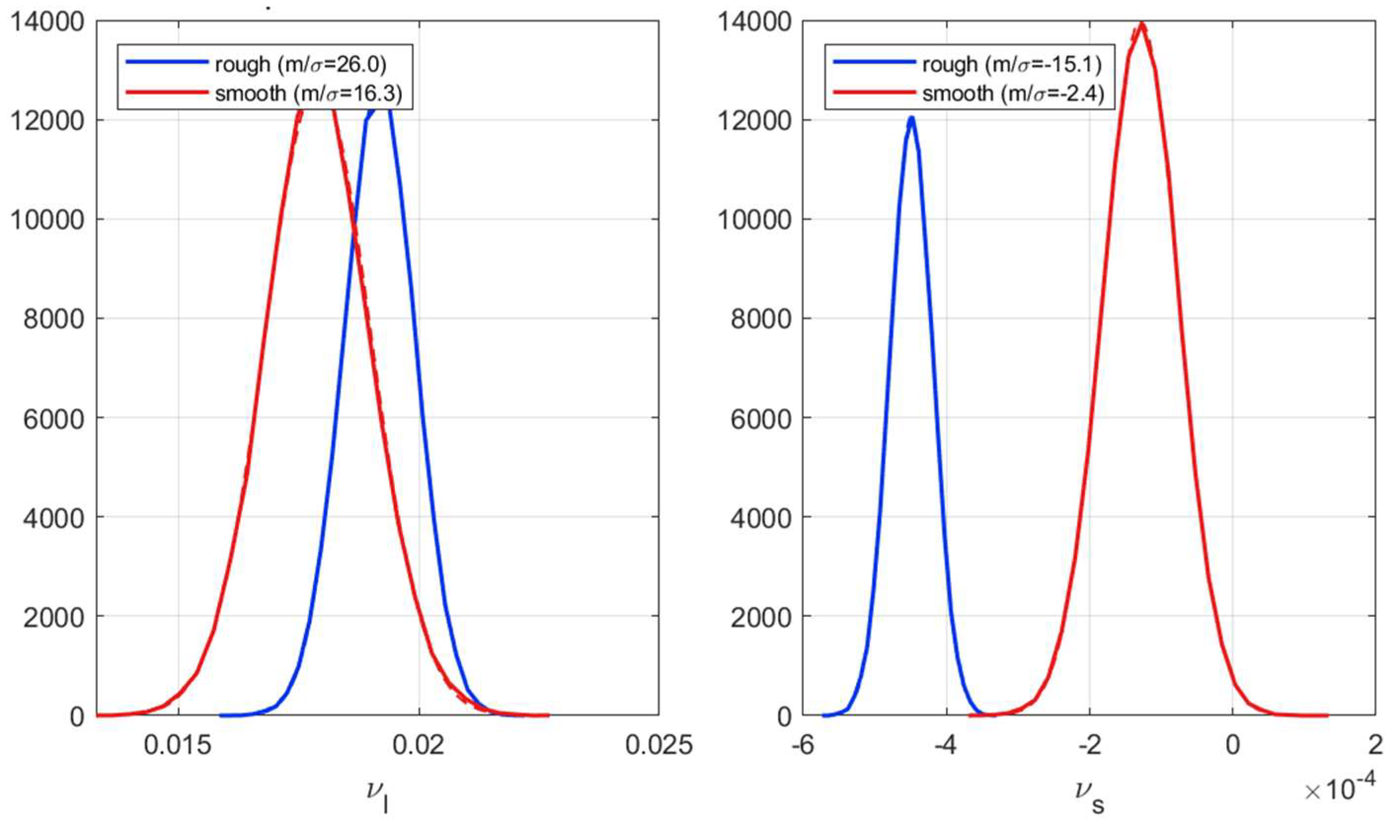
The linear models capture the dependence of the three HAF coefficients on load, temperature, and speed well: the coefficient of determination exceeds 0.93 for five of the six coefficient–surface combinations, reaching 0.98 for ν on smooth surfaces (Figure 12). The single exception is the hysteresis parameter h on rough surfaces (R2 = 0.76), whose fit is markedly poorer. Because each of these laws is estimated from seven operating conditions with four coefficients, leaving only three residual degrees of freedom, the adjusted coefficient of determination is also reported. The penalty it applies is far from negligible and is very unequal: it reduces R2 by only 0.02–0.05 when the fit is good, but by 0.24 for the hysteresis parameter on rough surfaces, where the adjusted R2 falls to 0.52. The generalized model in Section 7.2 is statistically better for this reason. It pools the two surface states and estimates fifteen coefficients from fourteen conditions, instead of twelve coefficients, and has stronger statistical support: its adjusted R2 loses only four to five points relative to R2 (0.85 for h, 0.89 for a, and 0.91 for ν) and remains above 0.85 for the three parameters.
Figure 12.
Bootstrap distributions of the coefficient of determination (R2) and of the adjusted coefficient of determination of the linear models, for the three HAF parameters (h, a, and ν) on rough discs (left) and smooth discs (right). Outlines show R2 and filled histograms show the adjusted R2, which penalizes the four coefficients estimated from seven conditions. Mean values: h—rough 0.76 (adjusted 0.52), smooth 0.97 (0.94); a—rough 0.94 (0.87), smooth 0.95 (0.90); ν—rough 0.94 (0.88), smooth 0.98 (0.96). Note that the horizontal scales of the two panels differ: the adjusted R2 of h on rough discs extends well below the range of the right-hand panel.
The signs and magnitudes of the coefficients are physically consistent. Load exerts the strongest and most systematic influence on h (positive 0.779 for rough and positive 1.455 for smooth surfaces), so the hysteresis parameter increases with contact pressure, whereas temperature acts in the opposite direction (negative −0.0147 and −0.0213), in line with the thinning of the lubricant film and the decrease in transition steepness as temperature rises. The friction level ν increases moderately with load (about 0.019) and decreases slightly with temperature and speed, while the attrition parameter a shows only weak dependencies on all three variables, with coefficients close to zero.
The bootstrap standard deviations quantify how the noise of the traction curves propagates to each coefficient; as noted above, they are not by themselves a measure of how firmly a dependency is established. Relative to their values, the coefficients of ν are the least affected by that noise, whereas those of h on rough surfaces are the most affected. The intercepts also reveal a pronounced baseline shift between surface states—most strikingly for h (1.49 for rough versus 0.09 for smooth), but also for a and ν, which shows that surface roughness affects the baseline levels of the coefficients rather than merely adding scatter. This observation motivates the generalized model of Section 7.2, where roughness is introduced explicitly as an additional variable rather than handled through two separate fits.
These separate laws are estimated from seven operating conditions with four coefficients each, which leaves only three residual degrees of freedom. Formal inference on them is correspondingly weak: with a Student t distribution on three degrees of freedom, the two-sided 5% threshold is 3.18, and only seven of the twenty-four coefficients reach it; for the hysteresis parameter on rough surfaces, none of the four reach the threshold, which is consistent with the low adjusted R2 of that fit. The surface-by-surface laws of this section are therefore presented as exploratory. They establish the signs and the approximate magnitudes of the effects, and they reveal the baseline shift between surface states that motivates the next section, but the inference on individual coefficients is deferred to the generalized model of Section 7.2, which estimates fifteen coefficients from fourteen conditions and therefore retains nine residual degrees of freedom.
Table 3.
Fitted coefficients of the linear models of h, a, and ν by surface state (load in GPa, temperature in °C, speed in m·s−1). Each cell gives the coefficient, the ratio m/σ of the bootstrap mean to its bootstrap standard deviation, and the Student t statistic with its two-sided p-value with three degrees of freedom. The two indicators answer different questions: m/σ measures how the noise of the traction curves propagates to the coefficient, whereas t tests whether the dependency is established by the seven conditions, and only the latter is a significance test. Coefficients significant at the 5% level (|t| > 3.18) are shown in bold. These surface-by-surface laws are exploratory; inference is based on the generalized model in Table 4.
7.2. Coefficient Modeling, Including Roughness
We now pool the two datasets and introduce the surface state as a binary variable (rough = 1 for rough discs, 0 for smooth), so that a single set of laws describes both surfaces:
where , , and are the roughness coefficients; the intercepts and the load, temperature, and speed coefficients retain the definitions given above. As before, each coefficient is estimated across the bootstrap replicates (Figure 13), thereby propagating the traction-curve noise; its significance, however, is assessed from the least-squares standard error, as explained below.
The uncertainties reported in Table 4 are least-squares standard errors computed on the fourteen conditions, and significance is assessed by a Student t test with nine degrees of freedom. This differs from the criterion used in the first version of this work, where the ratio of a bootstrap mean to its bootstrap standard deviation was compared with 1.96. There are two reasons for this change. First, the bootstrap standard deviation propagates the measurement noise of the traction curves but not the scatter of the fitted parameters about the linear law, and it is therefore systematically smaller by a factor of 1.2 to 4.1 depending on the coefficient. Second, with fourteen conditions and five coefficients, the reference distribution is a Student t with nine degrees of freedom, whose two-sided 5% threshold is 2.26 rather than 1.96. The standard errors obtained by least squares were confirmed by a bootstrap performed at the whole-curve level, which reproduced them to within a few percent.
Table 4.
Fitted coefficients of the generalized linear models, including roughness (rough = 1, smooth = 0), with load in GPa, temperature in °C, and speed in m·s−1. Each cell gives the coefficient, the ratio m/σ of the bootstrap mean to its bootstrap standard deviation, and the Student t statistic with its two-sided p-value with nine degrees of freedom. The bootstrap ratio propagates the measurement noise of the traction curves only, and is therefore systematically optimistic; the t statistic, based on the least-squares standard error, also accounts for the scatter of the fitted parameters about the law and provides the significance test. Coefficients significant at the 5% level (|t| > 2.26) are shown in bold.
Because fifteen coefficients are tested simultaneously, the significance levels were also examined under correction for multiple comparisons. Controlling the false discovery rate leaves the eleven significant coefficients unchanged, and the Bonferroni correction, which is the most conservative, retains ten of them; the six strongest effects—the roughness and load effects on ν, the load and temperature effects on a, and the temperature and roughness effects on h—remain significant with corrected p-values below 0.01.
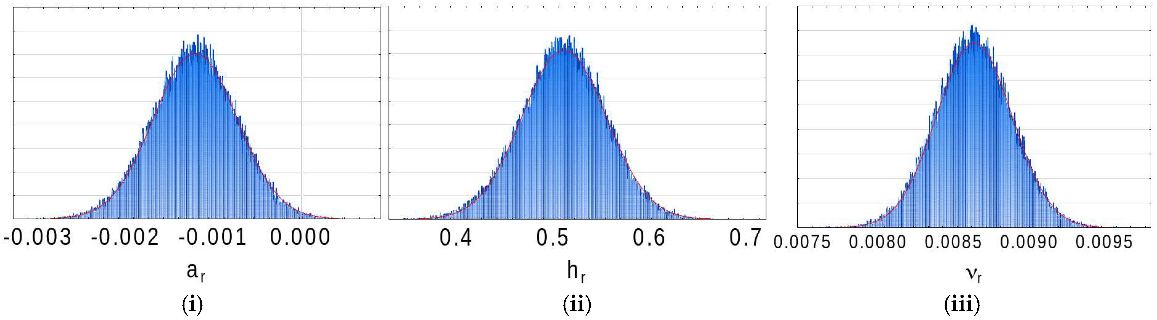
The generalized model, which pools the rough and smooth data and introduces roughness as a single binary variable, confirms the trends identified in Section 7.1. The signs of the load, temperature, and speed coefficients are unchanged: load increases the hysteresis h and the friction level ν and slightly decreases the attrition a, while temperature lowers both h and ν. Above all, the roughness term is highly significant for the friction level and for the hysteresis—0.0085 for ν (t = 7.98, p < 0.001) and 0.503 for h (t = 4.94, p < 0.001)—whereas the roughness effect on attrition is not statistically significant in the present data (−0.0011, t = −1.42, p = 0.19). Roughness therefore raises the hysteresis and the friction level, and both effects are substantial rather than secondary.
Compared with the two separate fits of Section 7.1, this single model is more parsimonious and is better supported statistically. Each of its three parameter laws estimates five coefficients from fourteen conditions, leaving nine residual degrees of freedom, compared with three for each separate fit, so that its adjusted coefficients of determination remain high—0.848 for h, 0.891 for a, and 0.911 for ν—whereas those of the separate fits fall as low as 0.53. Eleven of its fifteen coefficients are significant at the 5% level, and seven of them are significant at the 0.1% level. The four that are not are the intercepts of h and ν, the effect of speed on h, and the effect of roughness on a. For hysteresis in particular, the pooled model is markedly better than the rough-surface fit of Section 7.1 (R2 = 0.895 against 0.766), showing that the two surface states jointly stabilize an otherwise poorly constrained law.
Figure 13.
Bootstrap distributions of the roughness coefficient for (i) a, (ii) h, and (iii) ν—the effect introduced in the generalized model (Section 7.2). The effect is highly significant for the friction level and for the hysteresis, whereas its effect on attrition is not statistically significant in the present data (Table 4). The complete set of all coefficients (and the associated R2) is given in Appendix A, Figure A7.
7.3. The Complete Friction Model
The three linear laws can therefore be substituted into the HAF form. Replacing the three coefficients in Equation (10) by their expressions in the operating conditions gives Equations (19)–(21).
Written in full, this yields a single closed-form model of the friction coefficient as a function of load, temperature, speed, and surface state (Equation (22)).
Substituting the linear laws of h, a, and ν into the HAF equation yields a single closed-form expression that predicts the friction coefficient directly from the operating conditions and the surface state. Each coefficient is still estimated across the bootstrap replicates (Figure 14). The quality of this complete model is high: its coefficient of determination reaches R2 = 0.9957 ± 0.0004 (Figure 15), and the modeled friction coefficient plotted against the experimental value (Figure 16) falls almost exactly on the identity line for all six operating classes (rough and smooth surfaces at 1.2, 1.6, and 1.9 GPa). Because the friction coefficient is the quantity of primary engineering interest in tribology, this close agreement—obtained while explicitly incorporating the two first-order effects, roughness and contact pressure—shows that the compact three-parameter form describes the measured traction curves over the whole envelope, without implying that it resolves the physics of the contact.
Figure 14.
Bootstrap distributions of the complete-model roughness coefficient for (i) a, (ii) h, and (iii) ν—the roughness effect in the complete predictive model (Section 7.3). The complete set of the fifteen coefficient distributions is given in Appendix A, Figure A8.
Figure 15.
Bootstrap distribution of the coefficient of determination (R2) of the complete nonlinear predictive model with its fitting curve (red line). R2 = 0.9957 ± 0.0004 (mean ± standard deviation over the bootstrap samples): the single combined equation reproduces the friction coefficient across all operating conditions with a residual standard deviation of about 0.001.
Figure 16.
Modeled versus experimental tooth friction coefficient for the six operating classes (rough and smooth surfaces at contact pressures of 1.2, 1.6, and 1.9 GPa). The points align closely with the identity line, showing that the complete model predicts the friction coefficient accurately once the roughness and contact pressure effects are included. Inset: probability density of the modeled friction coefficient; the slight central trough separates the lower-friction and higher-friction populations of operating conditions.
The residuals of the complete model (Figure 17) confirm the quality of the regression. For both surface states, the residual distribution is near-Gaussian and centered on zero—a direct consequence of the least-squares criterion—with almost identical spreads (σ ≈ 0.001 in friction-coefficient units). This residual spread is a more informative measure of accuracy than the coefficient of determination, whose near-unit value partly reflects the wide range of friction values over which it is computed. The residuals are approximately Gaussian, centered on zero, and homoscedastic, with no evident systematic structure. These diagnostics support the adequacy of the fitted model over the tested conditions; Gaussianity itself is not a requirement of the Gauss–Markov theorem.
Figure 17.
Distribution of the model residuals (experimental minus modeled friction coefficient) for rough and smooth surfaces. Both distributions are near-Gaussian and centered on zero—a property of the least-squares fit—with nearly equal standard deviations (σ ≈ 0.0011 and 0.0013 for the two surface states), i.e., of the order of ±0.001 in friction-coefficient units. The approximately Gaussian, zero-mean, and homoscedastic residuals show no evident systematic structure over the tested conditions.
Figure 18 shows the measured traction curves, together with their reconstruction by the complete model over the whole set of operating conditions. The reconstruction is accurate for all observed curve shapes—steep or gradual, symmetric or markedly asymmetric—which is itself notable: a single three-parameter form accommodates the full variety of friction behaviors observed across pressures and surface states. Consistently with Section 7.1 and Section 7.2, twelve of the fifteen coefficients of the complete model are significant at the 95% level (Table 5). The only clear exceptions are the intercept of h and the roughness effect on a, with the intercept of ν being at the borderline. This again indicates that the hysteresis offset and the weak roughness–attrition coupling are the least-constrained terms.
Figure 18.
Experimental friction curves (points) and their reconstruction by the complete model (lines) for four representative operating conditions—(a) rough, 1.2 GPa, 80 °C, 20 m·s−1; (b) rough, 1.6 GPa, 100 °C, 20 m·s−1; (c) smooth, 1.6 GPa, 80 °C, 20 m·s−1; and (d) smooth, 1.9 GPa, 80 °C, 20 m·s−1—chosen to span the range of observed shapes, from a steep, nearly symmetric sigmoid to flatter, markedly asymmetric curves. The complete set for all operating conditions is given in Appendix A, Figure A9.
Table 5.
Coefficients of the complete nonlinear predictive model, obtained by substituting the linear laws of h, a, and ν into the HAF equation and reoptimizing the fifteen coefficients globally on the 350 experimental points. Each cell gives the coefficient, its standard error, and the Student t statistic with its two-sided p-value on 335 degrees of freedom. The coefficients differ from those of Table 4 because they result from a global reoptimization and not from a substitution of the laws in Table 4. The large number of degrees of freedom should be read with caution: the points from the same traction curve are not independent observations, so that the effective number of independent conditions remains fourteen and the significance levels reported here are correspondingly optimistic. Table 4 provides the more conservative significance assessment. Coefficients significant at the 5% level are shown in bold.
7.4. Validation on Unseen Operating Conditions
The coefficient of determination reported above is computed on the same points that were used to calibrate the model. It measures how well the model describes the data, not how well it predicts a condition that has not been tested. Since the practical purpose of the model is precisely to predict friction for untested combinations of load, temperature, speed, and surface state, its predictive ability was assessed by leave-one-condition-out cross-validation.
Each of the fourteen operating conditions was removed in turn. The three parametric laws were re-estimated on the thirteen remaining conditions only, and the friction curve of the excluded condition was then predicted from its operating variables alone. Neither the data points nor the fitted parameters of the excluded curve were used in the estimation, so the resulting error is a genuine prediction error. The procedure was repeated for the fourteen conditions, giving 350 predicted points in total; the construction of the associated prediction intervals is detailed in Appendix C.7.
Over the 350 points, the root mean square prediction error is 0.00203 in friction-coefficient units, compared to 0.00142 for the model fitted on all conditions, an increase of 43%. The mean absolute error is 0.00153, and the largest absolute error is 0.0089. The 95% prediction intervals contain 96% of the measured points, so the uncertainty attached to a prediction is realistic and, if anything, slightly conservative. Table 6 gives the four indicators condition by condition.
Table 6.
Leave-one-condition-out prediction error, condition by condition. n is the number of digitized points of the excluded curve. The last line pools the 350 predicted points.
Two features of Figure 19 deserve commentary. The conditions closest to the center of the experimental design—the reference point and the two neighboring pressures—are predicted almost as well as they are fitted, because removing them barely changes the estimated laws. The conditions at the edges of the design, in particular the lowest speed on rough discs and the lowest temperature on smooth discs, are predicted less accurately, which is expected since their removal deprives the corresponding law of one of its two extreme points. This is a property of the one-factor-at-a-time design rather than of the model.
Figure 19.
Root mean square error for each operating condition, when the model is fitted on all fourteen conditions (blue) and when the condition is left out of the estimation and predicted (orange). The prediction error remains of the same order as the fitting error for most conditions. The dotted vertical line separates the rough-disc conditions (left) from the smooth-disc conditions (right).
These results support characterizing the model as predictive rather than merely descriptive: it reproduces, within about 0.002 in terms of the friction coefficient, traction curves that played no part in its construction. The prediction error nevertheless remains of the same order as the residual scatter of the model, and predictions far outside the tested envelope should be treated with corresponding caution.
8. Prediction and Selection of Low-Friction Operating Conditions
Once the complete model has been established and validated (Section 7), it can be used as a predictive tool. A key advantage of the bootstrap is that it provides both point predictions and uncertainty intervals for the predicted friction coefficient: propagating the resampled coefficient sets through the model equation yields, for any operating condition, a full distribution of predicted friction rather than a single value. This section uses that capability in two stages, first to quantify the uncertainty of the prediction over the whole operating envelope, then to use the model to explore operating conditions and to identify those that minimize friction.
The engineering motivation is direct: the tooth friction coefficient is an important input in analyses of both the transmission efficiency and tooth-surface damage (scuffing and wear) of the teeth. Being able to predict friction, with quantified confidence, for arbitrary combinations of load, temperature, speed, and surface state therefore opens the way to selecting operating conditions that reduce the maximum friction coefficient, thereby supporting assessments of surface damage risk.
Figure 20 shows the density of the predicted friction coefficient obtained when the bootstrap coefficient sets are propagated through the model across the entire operating envelope. Rather than a single predicted value, the model returns a distribution that quantifies prediction uncertainty; its predictive performance is evaluated independently by the cross-validation in Section 7.4. Separating the surface states shows that rough surfaces shift the prediction toward higher friction, and that the two populations only partly overlap, consistent with the strong, significant roughness terms of Section 7.2.
Figure 20.
Bootstrap distribution (probability density) of the friction coefficient predicted by the complete model over the whole operating envelope: rough and smooth surfaces together, smooth surfaces only, and rough surfaces only. Each density combines variation across the operating envelope with bootstrap parameter uncertainty; it is not a pointwise confidence interval.
Because the complete model is a continuous, closed-form function of the operating parameters, it can generate a friction curve for any combination of load, temperature, speed, and surface state—not only at the measured points but also at intermediate combinations within the tested operating envelope. Figure 21 illustrates this by sweeping one parameter at a time: each curve corresponds to a different operating condition, and the family of curves maps how the friction behavior evolves as the conditions change. This is the model’s predictive, interpolative use: it turns a set of discrete measurements into a continuous design surface.
Figure 21.
Predicted friction curves obtained by varying the operating parameters (the entrainment speed at the reference contact pressure of 1.6 GPa and reference temperature of 80 °C) for smooth surfaces. Because the model is continuous in load, temperature, speed, and roughness, it generates a friction curve for any combination of conditions, including intermediate combinations not tested directly, provided that they remain within the experimental envelope. The four panels differ only by the entrainment speed, given in each panel title, and are read as a single continuous family.
Scanning the operating space with the model makes it possible to single out the conditions that minimize or maximize friction. Figure 22 contrasts the best, median, and worst cases. The friction coefficient compared between conditions is the maximum of the predicted curve over the swept range of the slide-to-roll ratio. The difference between conditions is large. On smooth discs, the best condition—a low load of 1.2 GPa, a high temperature of 100 °C, and a high speed of 30 m·s−1—gives a maximum friction coefficient of 0.0049, whereas the worst (1.9 GPa, 40 °C, and 10 m·s−1) reaches 0.0304, which is six times higher. Including rough discs, the worst condition of the whole envelope reaches 0.0388, which is eight times the best. Low contact pressure combined with high temperature and high speed therefore reduces friction, in agreement with the coefficient signs of Section 7: friction grows with contact pressure and decreases as temperature and, to a lesser extent, speed increase.
Figure 22.
Predicted friction curves for the best, median, and worst operating conditions of the envelope on smooth discs. The envelope was scanned on the grid used throughout Section 8 (contact pressure from 1.2 to 1.9 GPa in steps of 0.1, temperature from 40 to 100 °C in steps of 10, and speed from 10 to 30 m·s−1 in steps of 5, i.e., 280 conditions per surface state), and the conditions were ranked by the maximum of the predicted friction coefficient over the swept range of the slide-to-roll ratio, which is the quantity marked on each curve. The best condition (1.2 GPa, 100 °C, and 30 m·s−1) gives 0.0049, the worst (1.9 GPa, 40 °C, and 10 m·s−1) gives 0.0304, and the median condition of the ranking (1.8 GPa, 70 °C, and 30 m·s−1) gives 0.0184.
More generally, because the model is a smooth and differentiable expression of the operating parameters, its gradient with respect to load, temperature, and speed can be obtained analytically. The optimum reported above was obtained by scanning the operating envelope, and the resulting combination was not among the measured operating conditions; it is therefore a model prediction rather than a selection from the measured cases. Beyond this scan, the differentiability of the expression opens the way to gradient-descent or quasi-Newton optimization, which would locate the optimum directly rather than on a grid; since the bootstrap provides the prediction uncertainty, such a search could be carried out on a conservative upper bound of the friction rather than on its point estimate alone. This route has not been pursued here and is left for future work. Even in its present form, the model can serve as a design tool, since it indicates the loads, speeds, and temperatures that lower tooth friction without further testing—bearing in mind that a lower friction coefficient does not by itself guarantee a lower power loss, which also depends on the transmitted load and on the sliding speed.
9. Discussion
The prediction of the tooth friction coefficient has traditionally been approached along two lines. The first is physics-based: elastohydrodynamic (EHL) models resolve the lubricant film and the shear stress in the contact, from which the friction coefficient is derived [9,17]; in gear practice, these are often condensed into regression formulae fitted to large sets of EHL computations, as in the widely used model of Xu and Kahraman [18], the partial EHL model of Arana et al. [19], or recent multi-tooth tribo-dynamic and local-to-mean friction models [10,11]. The second line is empirical: closed-form expressions relating the mean friction coefficient to load, sliding velocity, viscosity, and roughness, from the classical laws of Benedict and Kelley [20] and Kelley and Lemanski [21] to the modified Hersey formula of Fernandes et al. [22]. The phenomenological HAF model examined here, which extends the semi-empirical approach of Quiban et al. [1], does not fit neatly into either category: it imposes the shape of the traction curve through three interpretable parameters and then lets the operating conditions act on those parameters.
Imposing the sigmoidal shape is not arbitrary curve-fitting. The rheology of an EHL contact produces a traction curve that rises approximately linearly at a low slide-to-roll ratio (Newtonian regime), then shear-thins, and finally saturates at a limiting shear stress [17,23]; it is that limiting shear stress, and its dependence on pressure and temperature, that sets the maximum traction. The three HAF parameters describe corresponding features of the curve: h governs the steepness of the transition (the hysteresis of the rolling–sliding contact), a governs the residual slope of the plateau (attrition), and ν governs the amplitude (the overall friction level). The phenomenological form therefore compactly encodes the qualitative physics that full EHL models compute in detail.
The principal advantage of this approach is statistical identifiability. Physics-based models require a large number of uncertain inputs—lubricant rheology, film thickness, thermal properties, and roughness spectra—and they are ultimately calibrated on the very traction curves they aim to reproduce [9,17]. It has recently been shown that a traction curve does not contain enough information to recover the underlying rheological parameters uniquely: markedly different parameter sets reproduce the same curve within experimental error, and the extracted values are system-dependent [24,25]. This is the signature of an ill-posed inverse problem, of the kind described more generally as a “sloppy” model, in which many combinations of parameters are indistinguishable from the data [26,27]. Fixing the functional form and reducing the description to three parameters sidesteps this degeneracy: the bootstrap distributions obtained here are near-Gaussian, weakly correlated, and, for most regression coefficients, significantly different from zero (Table 4). The three HAF parameters are identifiable within the present dataset, whereas the larger parameter sets of full physical models may not be uniquely recoverable from a single traction curve.
The bootstrap is central to this uncertainty analysis. By resampling the residuals and refitting the model, it provides empirical estimates of coefficient uncertainty [13] without assuming normal errors or linearizing the model. Beyond confidence intervals, it underpins the residual diagnostics of the complete model: the residuals are approximately Gaussian, centered on zero, and homoscedastic, with no evident systematic structure. Such an uncertainty budget is rarely reported for gear friction models, which are usually presented as point formulae; here, it is precisely what supports predictive use of the model, with uncertainty intervals for the predicted friction.
The analysis confirms that surface roughness and contact pressure are first-order effects on tooth friction, in line with earlier experimental evidence [2,3] and with recent studies relating roughness and its orientation to the friction coefficient [28,29,30]. When roughness is introduced explicitly (Section 7.2), its coefficient is highly significant for the friction level and for the hysteresis, while its effect on attrition is not statistically significant in the present data, and the pooled model even improves the description of the hysteresis parameter relative to separate fits. Load increases both the hysteresis and the friction level, whereas temperature lowers them, consistent with the thinning of the film and the reduction in the limiting shear stress as temperature rises [17]. The speed dependence, by contrast, is weak and often not significant, which is consistent with the hysteresis being governed primarily by pressure and temperature over the range tested.
Because friction is a major contributor to load-dependent power loss in gears and is associated with surface damage such as scuffing and wear [31,32,33], a predictive and differentiable friction law has direct engineering value. The complete model reproduces the measured friction coefficient with a residual standard deviation of about 0.001 (R2 ≈ 0.996). Being a closed-form differentiable function of load, temperature, and speed, the model lends itself to gradient-based optimization of the operating conditions. Combined with the bootstrap prediction intervals, this makes it possible to search for the conditions that minimize friction while accounting for the uncertainty of the prediction. In the spirit of gearbox efficiency optimization studies, this is increasingly relevant for electrified transmissions [5,34,35].
The friction coefficient is not the whole story, and the distinction deserves to be made explicitly. Frictional power loss in a gear mesh is the integral of the product of the normal load, the friction coefficient, and the sliding velocity along the path of contact [33,34]. A low friction coefficient therefore does not by itself guarantee a low power loss. Increasing the entrainment speed lowers the friction coefficient, as the present model and the literature both show, but it also increases the sliding velocity that multiplies it. Minimizing the friction coefficient and minimizing the dissipated power are therefore two distinct objectives.
This does not make the friction coefficient a secondary quantity. Within that integral, the normal load and the sliding velocity are set by the gear geometry and the operating point, whereas the friction coefficient is the only term that depends on the lubricant, the temperature, and the surface finish. It is thus a key tribological input, and it is the quantity that a model such as the present one can supply to a power loss computation, with the remaining terms being provided by the kinematics of the mesh.
The friction coefficient also enters the standard criteria for surface damage directly rather than indirectly. The scuffing risk is assessed in ISO/TS 6336-20 [36] through Blok’s contact temperature concept, in which the flash temperature is computed from the friction coefficient, the normal load, and the sliding velocity, and the standard evaluates the maximum contact temperature along the path of contact. Micropitting is assessed in ISO/TS 6336-22 [37] through the minimum specific film thickness, and the procedure introduces a sliding parameter that shifts the evaluation to the region of highest sliding, where micropitting is observed [38]. Both damage criteria are therefore particularly sensitive to conditions of a large slide-to-roll ratio, in agreement with the practical observation that scuffing occurs near the tip or the root of the tooth rather than near the pitch point, where sliding vanishes.
The optimization in Section 8 should therefore be read with its objective made explicit. The quantity minimized is the maximum of the predicted friction curve over the swept range of the slide-to-roll ratio, and the objective is not the minimization of power loss but the reduction of the risk of surface damage. That maximum is reached at a large slide-to-roll ratio, which is where the flash temperature and the asperity shear are largest, and it is therefore the quantity that governs the scuffing and micropitting criteria of the standards cited above. Selecting operating conditions that lower it is a defensible design objective in its own right, distinct from minimizing the dissipated power, which would require the load and sliding distributions of a specific gear geometry and is not attempted here.
It is useful to situate the model between two extremes. Fully physical EHL models are the most detailed but, as discussed, are difficult to identify and computationally demanding; purely data-driven surrogates, such as the neural network and data-driven friction models now appearing in the literature [6,7,39], can be accurate but are opaque and give no physical reading of their parameters. The HAF model occupies a useful middle ground: it attains a close fit while retaining three parameters that each carry a clear tribological interpretation.
Several limitations should be kept in mind. The coefficients are specific to a given lubricant–material pair, and the friction levels measured here differ substantially from those obtained by Diab et al. on a different oil [9], so the calibration is not universal and must be repeated for other systems. The linear laws relating the parameters to the operating variables are local approximations, valid within the tested envelope; extrapolation far beyond it should be treated with caution. Roughness has been described here only through a binary state (smooth/rough); relating the HAF parameters to quantitative roughness descriptors is a natural extension. Finally, the coefficient uncertainties reported in the tables were, for the present manuscript, estimated from the bootstrap histograms and should be regarded as close approximations rather than exact figures.
The roughness enters the generalized model as a binary variable, and this deserves some commentary. With only two surface states, binary coding and continuous coding are mathematically equivalent: two levels define a single straight line, so that replacing the indicator with any measured roughness descriptor would yield the same model up to a change of scale and produce the same predictions. The binary description is therefore not a simplification of richer available information; it is the only information that two levels can carry. The limitation lies not in the coding but in the design: identifying which roughness descriptor governs the HAF parameters, testing whether the dependence is linear, and determining at which scale the topography acts all require at least three levels of roughness. Until such data are available, the model should be read as applying to two well-characterized surface finishes—a fine ground surface and a rough ground surface representative of gear flanks—rather than as a continuous law of roughness. Complementary tests covering several levels of roughness are underway and are intended to express each of the three HAF parameters as a function of measured roughness descriptors; the open question is then which descriptors, and at which scale, carry the dependence.
These limitations also outline the way forward. Because the three parameters are robust and identifiable, they can serve as reliable targets against which physics-based or numerical models are tested: rather than calibrating a physical model directly on a traction curve—an ill-posed task [24]—one can ask which physical ingredients reproduce the measured h, a, and ν, and their dependence on the operating conditions. Establishing that link, together with the use of real roughness descriptors, is the subject of ongoing work.
10. Conclusions
This work has examined a three-parameter phenomenological model (HAF) of the tooth friction coefficient, whose parameters have explicit tribological interpretations: the hysteresis h, the attrition a, and the friction level ν. The residual-resampling bootstrap (BIG) established in the companion paper [8] was used to quantify the uncertainty of the coefficients, and it yielded near-Gaussian, weakly correlated distributions, consistent with stable parameter estimation in the present dataset.
The dependence of the three parameters on load, temperature, speed, and surface roughness was described by simple linear laws. Eleven of the fifteen coefficients of the combined model are significantly different from zero at the 95% level, and the coefficients of determination of the individual laws exceed 0.93 for five of the six parameter–surface combinations, the exception being the hysteresis parameter on rough surfaces (R2 = 0.76). Introducing roughness explicitly in a single combined model quantified its effect—the roughness coefficient for ν reached t = 7.98—and improved the description of the hysteresis parameter. Substituting these linear laws into the HAF equation produced a complete, closed-form predictive model that reproduces the measured friction coefficient with a residual standard deviation of σ ≈ 0.001 in friction-coefficient units (R2 = 0.9957 ± 0.0004), with approximately Gaussian, zero-mean, and homoscedastic residuals that show no evident systematic structure.
Because the complete model is differentiable and its predictions come with bootstrap confidence intervals, it can be used to predict friction throughout the tested operating envelope and, through gradient-based optimization, to identify the operating conditions that minimize friction. A low friction coefficient does not by itself guarantee a low power loss, since the dissipated power also depends on the transmitted load and on the sliding speed; the model provides the friction coefficient, which is one factor in that product. The compactness and identifiability of the three-parameter form are its principal strengths: unlike heavily parameterized physical models, whose parameters cannot generally be recovered uniquely from a traction curve, the HAF parameters are robustly estimated and physically interpretable.
Two main directions for future work follow from this study. The first is to replace the binary smooth/rough description with a quantitative characterization of the surface topography. Ongoing work suggests that measured roughness parameters can be introduced into the same modeling framework and aims to identify which roughness descriptors, and at which scales, govern the three HAF parameters.
The second, more fundamental, direction is to use physics-based (EHL) simulation to clarify how the underlying physical ingredients act on h, a, and ν. Rather than calibrating a physical model directly on the traction curves, an ill-posed and poorly identifiable task [24], the robust, identifiable HAF parameters can serve as targets that a physical or numerical model must reproduce. This inverts the usual procedure and offers a principled way to assess the statistical robustness and the physical significance of the coefficients, ultimately bridging the phenomenological and physics-based descriptions of tooth friction.
Supplementary Materials
The following supporting information can be downloaded at: https://www.mdpi.com/article/10.3390/technologies14090586/s1, the reproducibility program in MATLAB/Octave (HAF_model.m) and Python (haf_model.py), the input dataset (SRR_frot_data.csv), a user guide for both implementations, and the complete set of generated tables and figures in their native resolution.
Author Contributions
Methodology, M.B.; Software, M.B.; Validation, F.V. and C.C.; Formal Analysis, M.B.; Investigation, M.B., J.L., E.C., Y.D., T.T., C.C., and F.V.; Data Curation, J.L.; Writing—Original Draft Preparation, M.B. and J.L.; Writing—Review and Editing, M.B., J.L., and F.V.; Visualization, J.L.; Supervision, M.B. All authors have read and agreed to the published version of the manuscript.
Funding
This work was carried out within the CapTrack project, a Just Transition Fund project (number 7A1B0040) co-funded by the European Union through the 2021–2027 regional program of the Hauts-de-France Region, France (grant agreement under signature), and supported also by SNCF Réseau. Views and opinions expressed are those of the authors only and do not necessarily reflect those of the European Union or of the granting authority. Neither the European Union nor the granting authority can be held responsible for them.
Institutional Review Board Statement
Not applicable.
Informed Consent Statement
Not applicable.
Data Availability Statement
The digitized traction data and the MATLAB program (R2025b) used to fit the HAF model, perform the bootstrap analysis, and generate all tables and figures are provided as Supplementary Materials (SRR_frot_data.csv, digitized from the published figures of [1], and HAF_model.m). The program requires only base MATLAB (R2016b or later) and also runs without modification under GNU Octave; no additional toolboxes are required. It reproduces Table 1, Table 2, Table 3 and Table 4 and Figure 1, Figure 2, Figure 3, Figure 4, Figure 5, Figure 6, Figure 7, Figure 8, Figure 9, Figure 10, Figure 11, Figure 12, Figure 13, Figure 14, Figure 15, Figure 16, Figure 17, Figure 18, Figure 19, Figure 20, Figure 21 and Figure 22, together with their complete per-condition sets in Appendix A. With the fixed random seed provided, the results are fully deterministic and reproducible. The code is released under the MIT License.
Conflicts of Interest
The authors declare no conflicts of interest.
Nomenclature
| HAF friction model | |
| SRR | slide-to-roll ratio, expressed in percentage points (%) |
| F(SRR) | tooth friction coefficient predicted by the model (–) |
| ν | friction-level parameter of the HAF model (–) |
| h | hysteresis parameter of the HAF model (%−1) |
| a | attrition parameter of the HAF model (%−1) |
| Operating conditions | |
| Load | maximum Hertzian contact pressure (GPa) |
| Temperature | operating (bulk) temperature (°C) |
| Speed | mean entrainment speed (m/s) |
| Rough | surface-roughness state (boolean: 0 = smooth, 1 = rough) |
| Linear coefficient models (Section 7) | |
| hi, ai, νi | model intercepts (%−1 for h and a, dimensionless for ν) |
| hl, al, νl | load coefficients (%−1·GPa−1 for h and a, GPa−1 for ν) |
| ht, at, νt | temperature coefficients (%−1·°C−1 for h and a, °C−1 for ν) |
| hs, as, νs | speed coefficients (%−1·(m/s)−1 for h and a, (m/s)−1 for ν) |
| hᵣ, aᵣ, νᵣ | roughness coefficients (%−1 for h and a, dimensionless for ν) |
| ε | residual (error) term of a linear model (–) |
| Statistics and bootstrap | |
| , , | bootstrap point estimates of h, a and ν (same units as the parameters) |
| R2 | coefficient of determination of a linear model (–) |
| σ | bootstrap standard deviation of a coefficient (coefficient unit) |
| m/σ | ratio of a bootstrap coefficient mean to its bootstrap standard deviation; not a Student t statistic (–) |
| N | number of bootstrap resamples (–) |
Appendix A. Complete Figure Sets
For readability, the figures of the main text show a representative subset of the results. This appendix reproduces, for every operating condition, the complete set of outputs with the original table layout (surface state, contact pressure, temperature, and speed).
Appendix A.1. Response Surfaces of the SSE (Complete Set of Figure 6)
Figure A1.
Response surface plots of the SSE versus the HAF parameters (ν, a, and h) for both smooth and rough surfaces at the three contact pressures, three temperatures, and three speeds. Each row corresponds to one operating condition; the three views show the ν–a, ν–h, and a–h parameter pairs. A single, well-defined minimum is observed in every case.
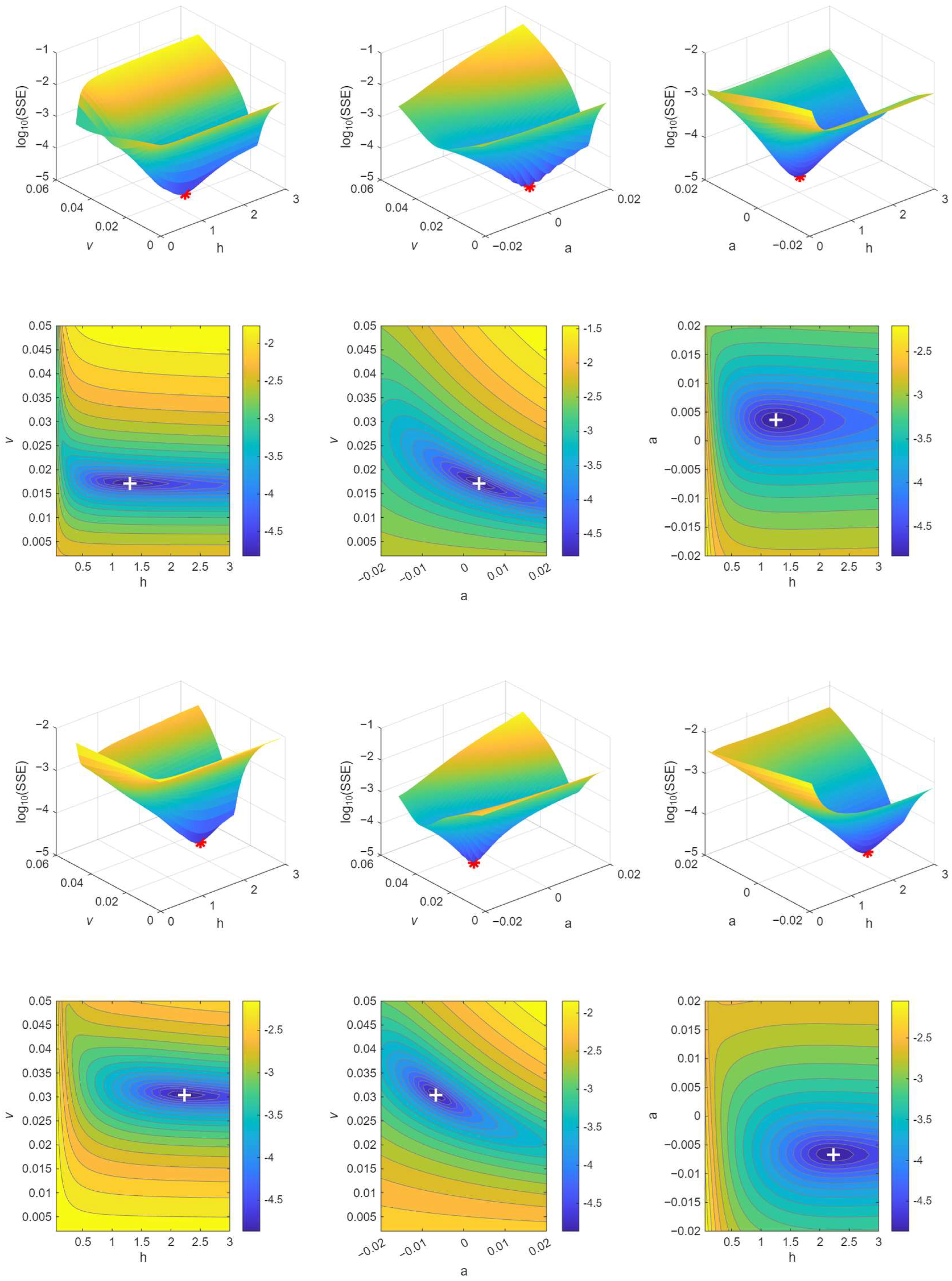
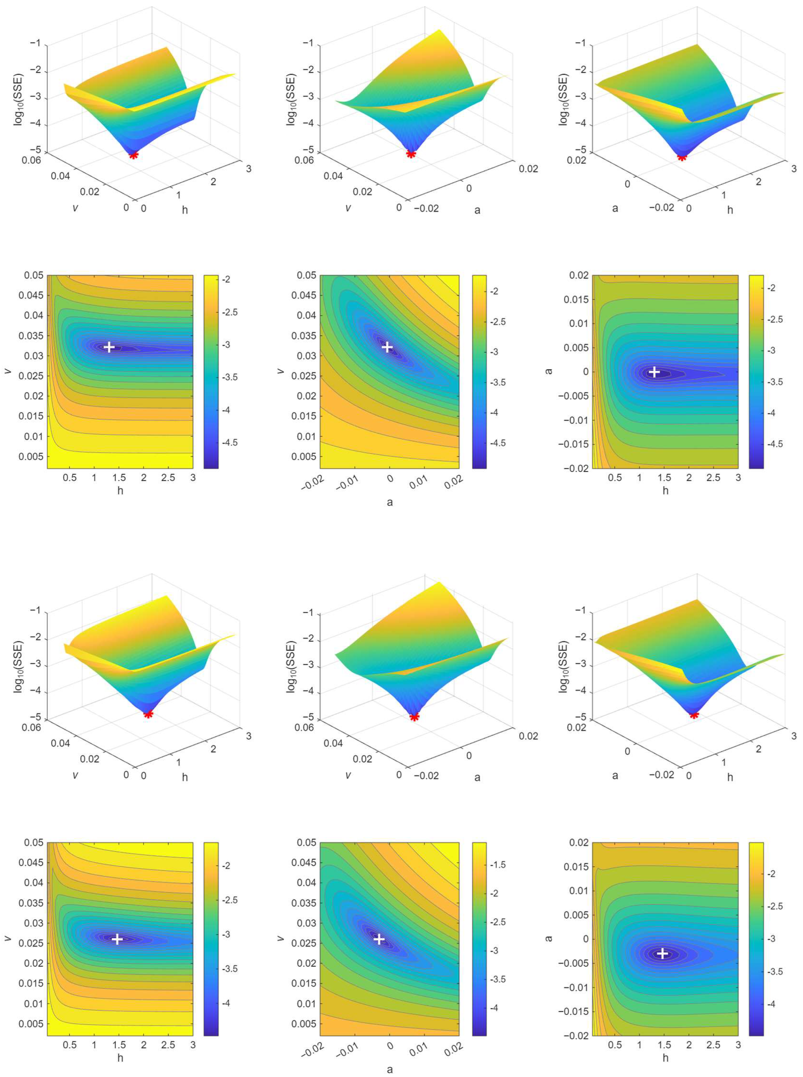
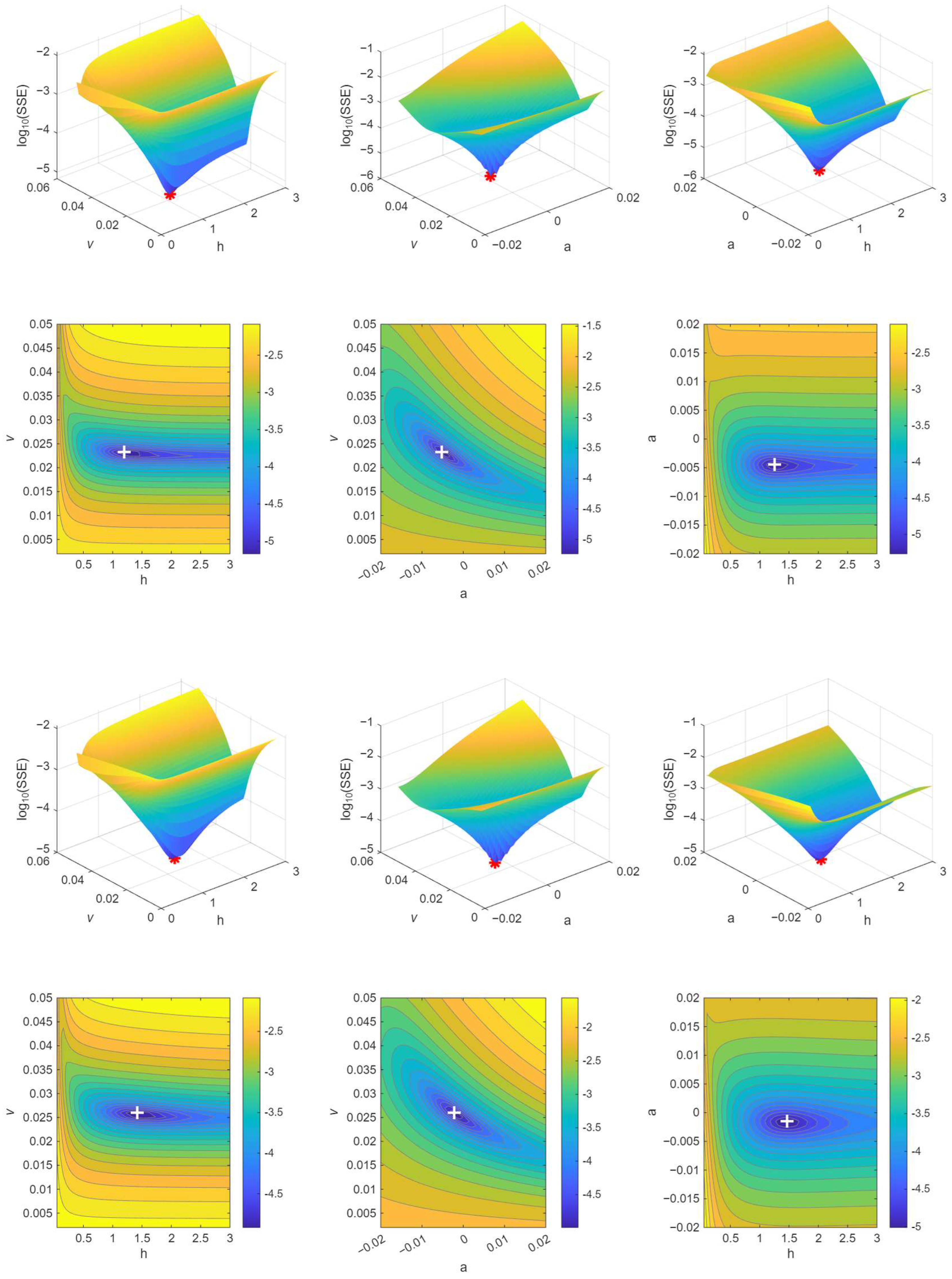
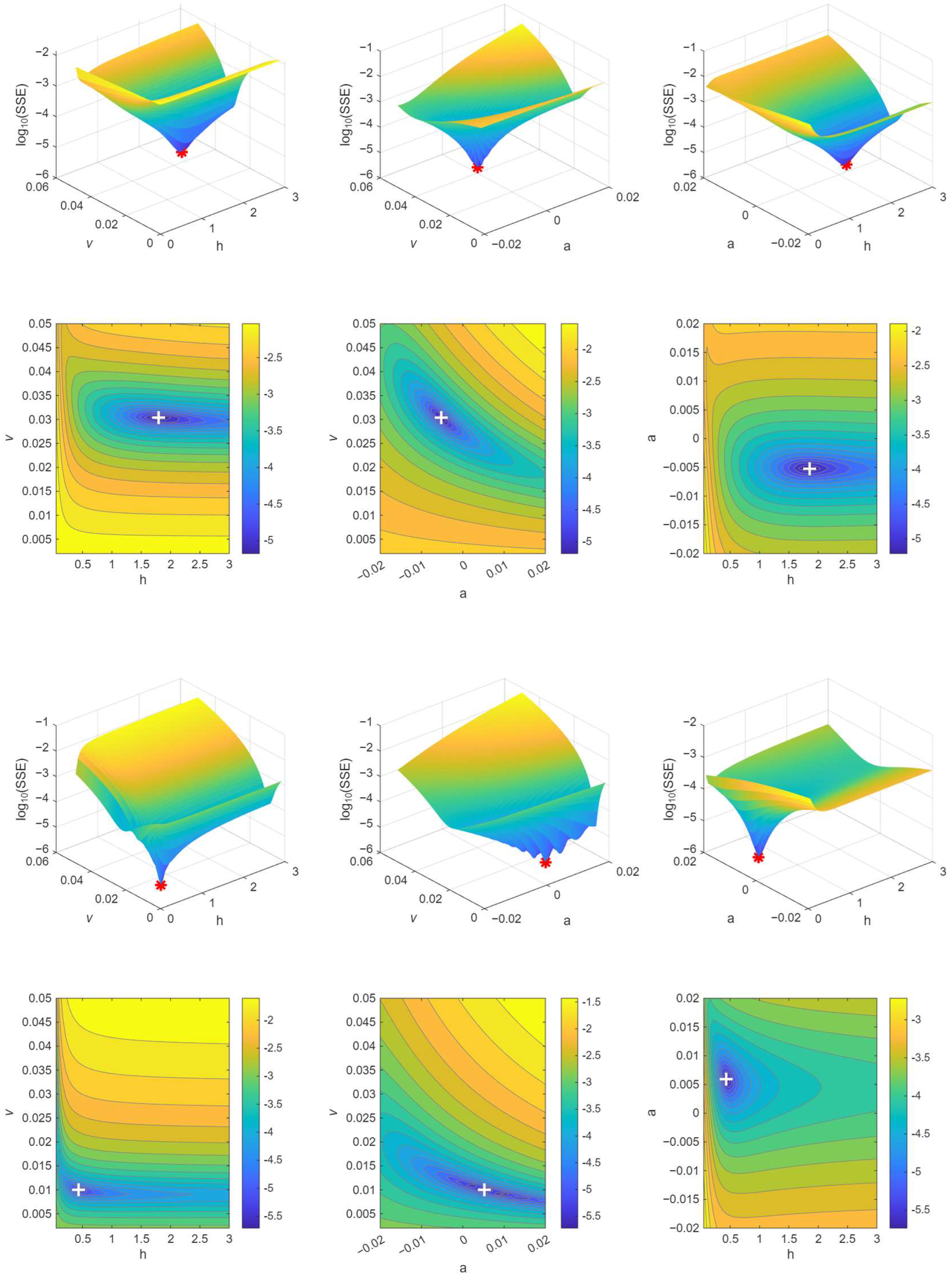
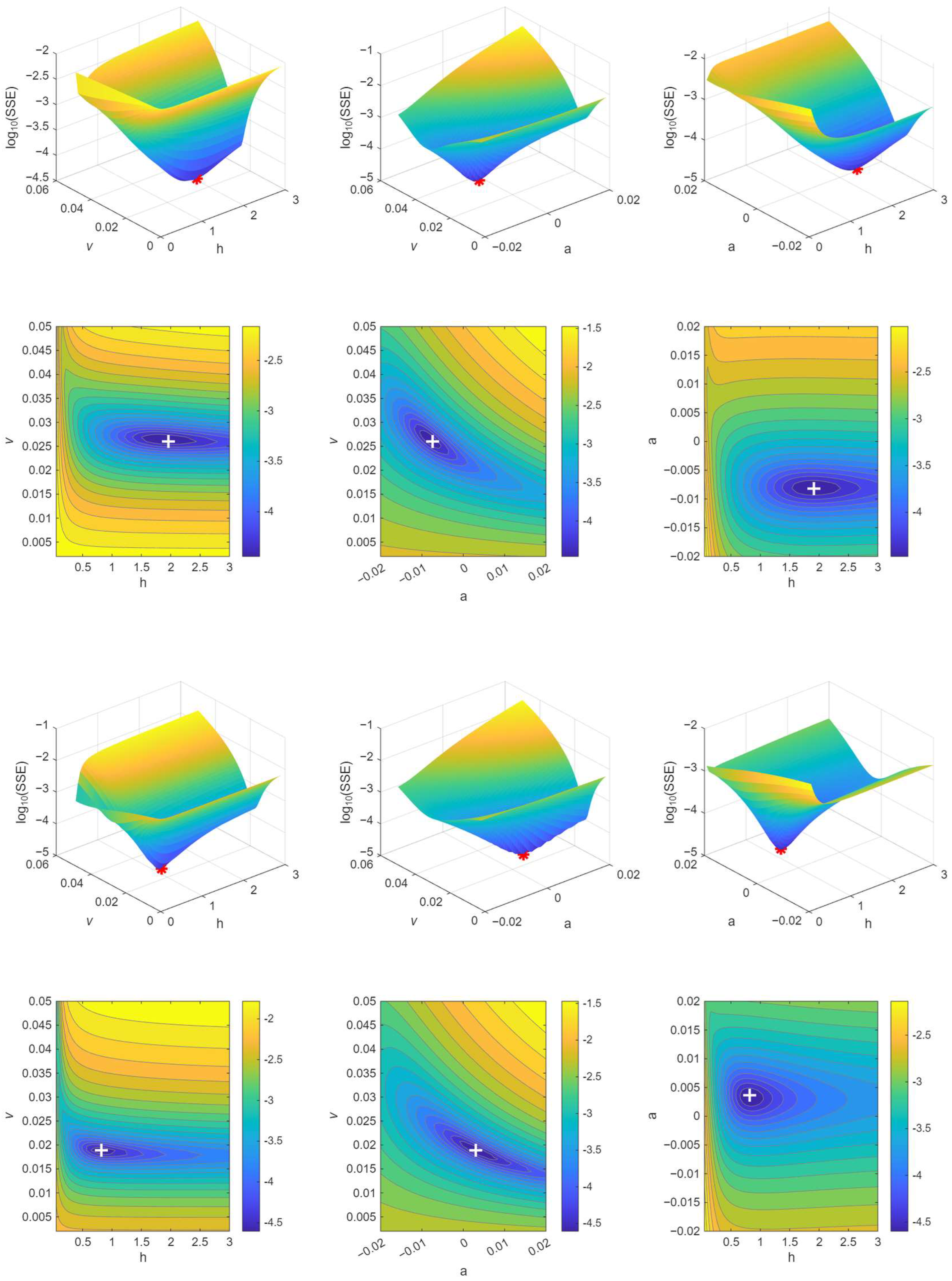
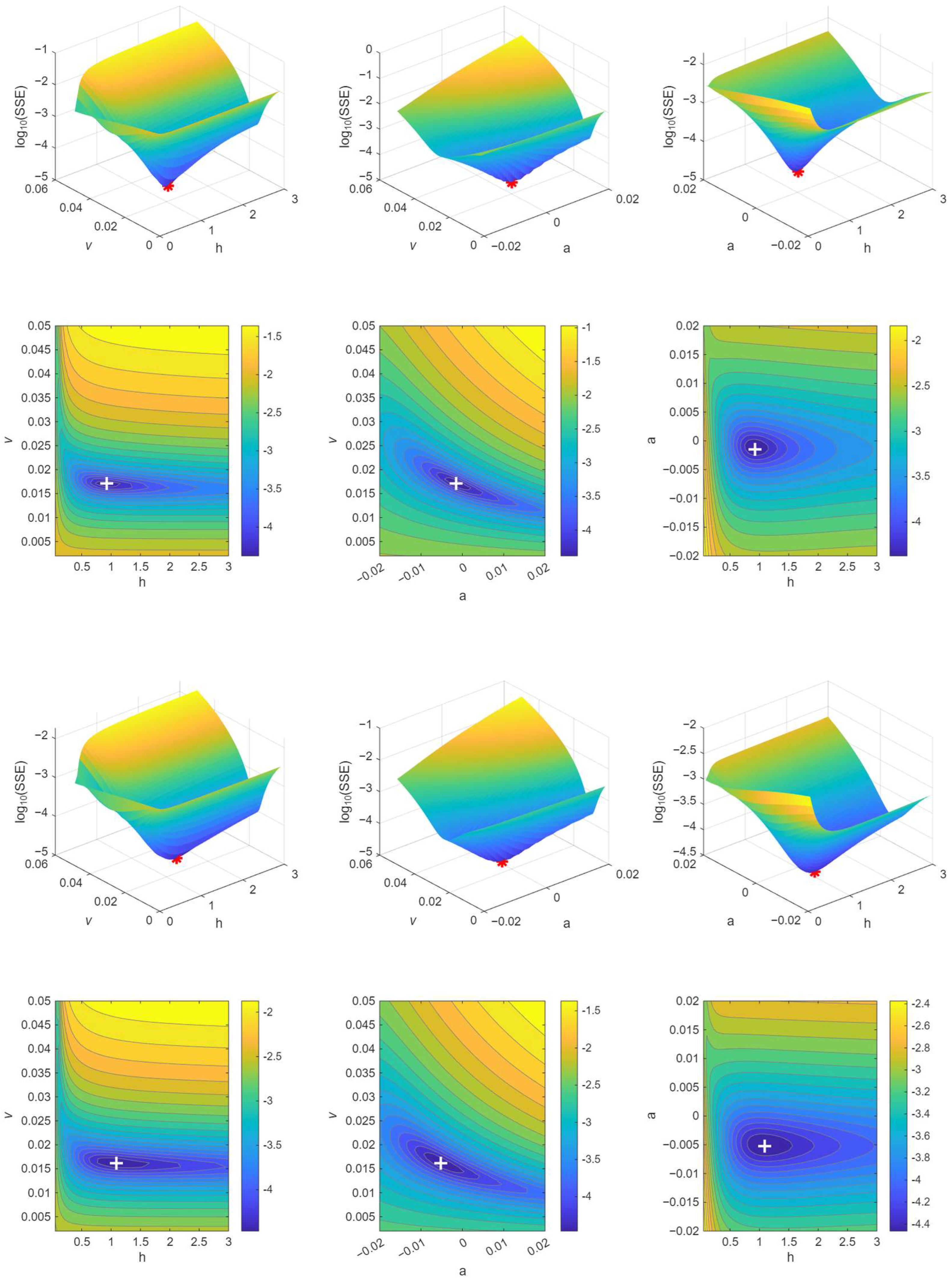
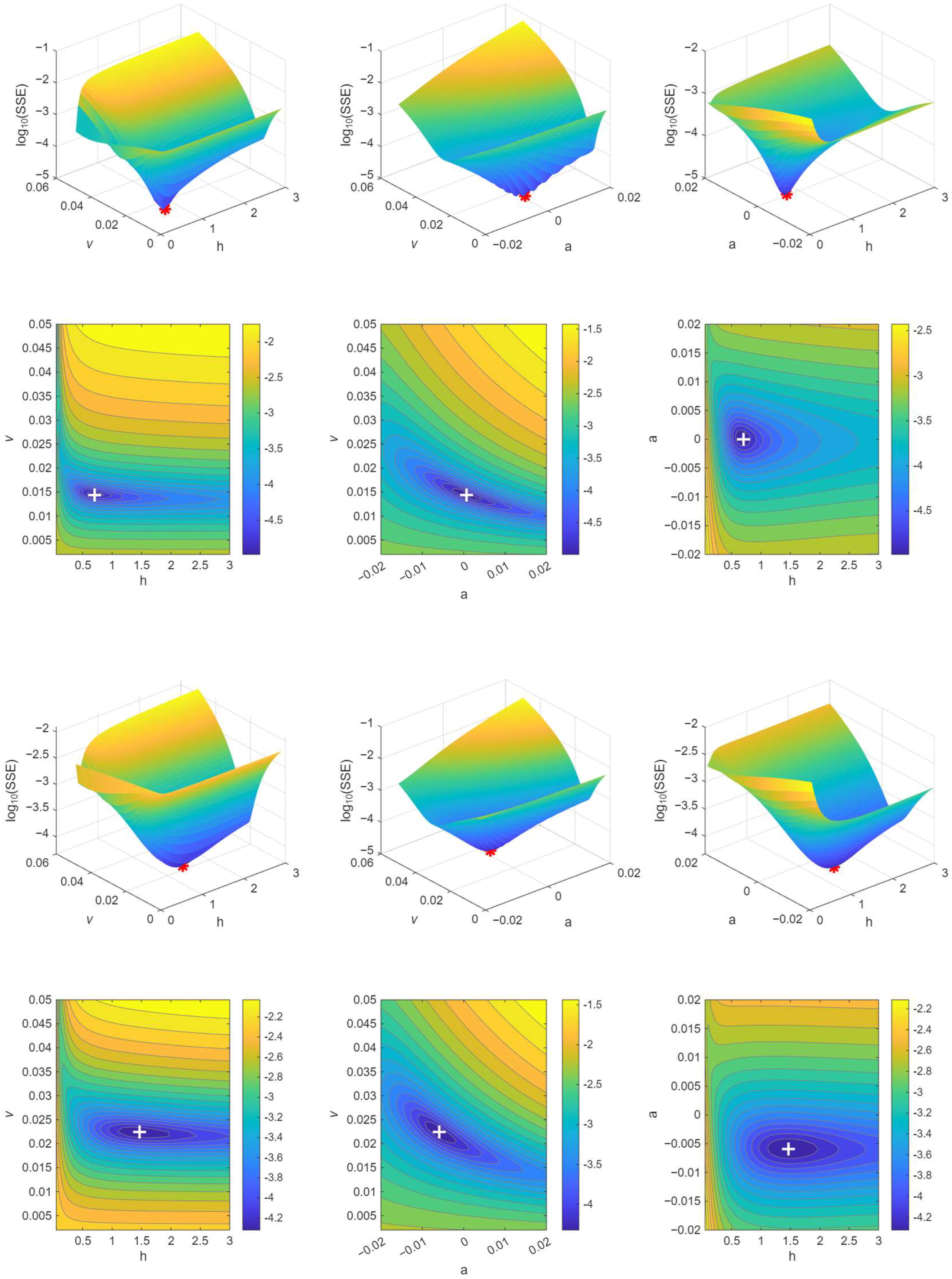
Appendix A.2. Probability Density Plots—Experimental SRR Sampling (Complete Set of Figure 7)
Figure A2.
Probability density of the bootstrapped friction points along the friction–SRR curve (non-uniform SRR sampling). The density is concentrated at the asymptotes and is thin along the rising branch of the sigmoid, where the h parameter is least supported by data.
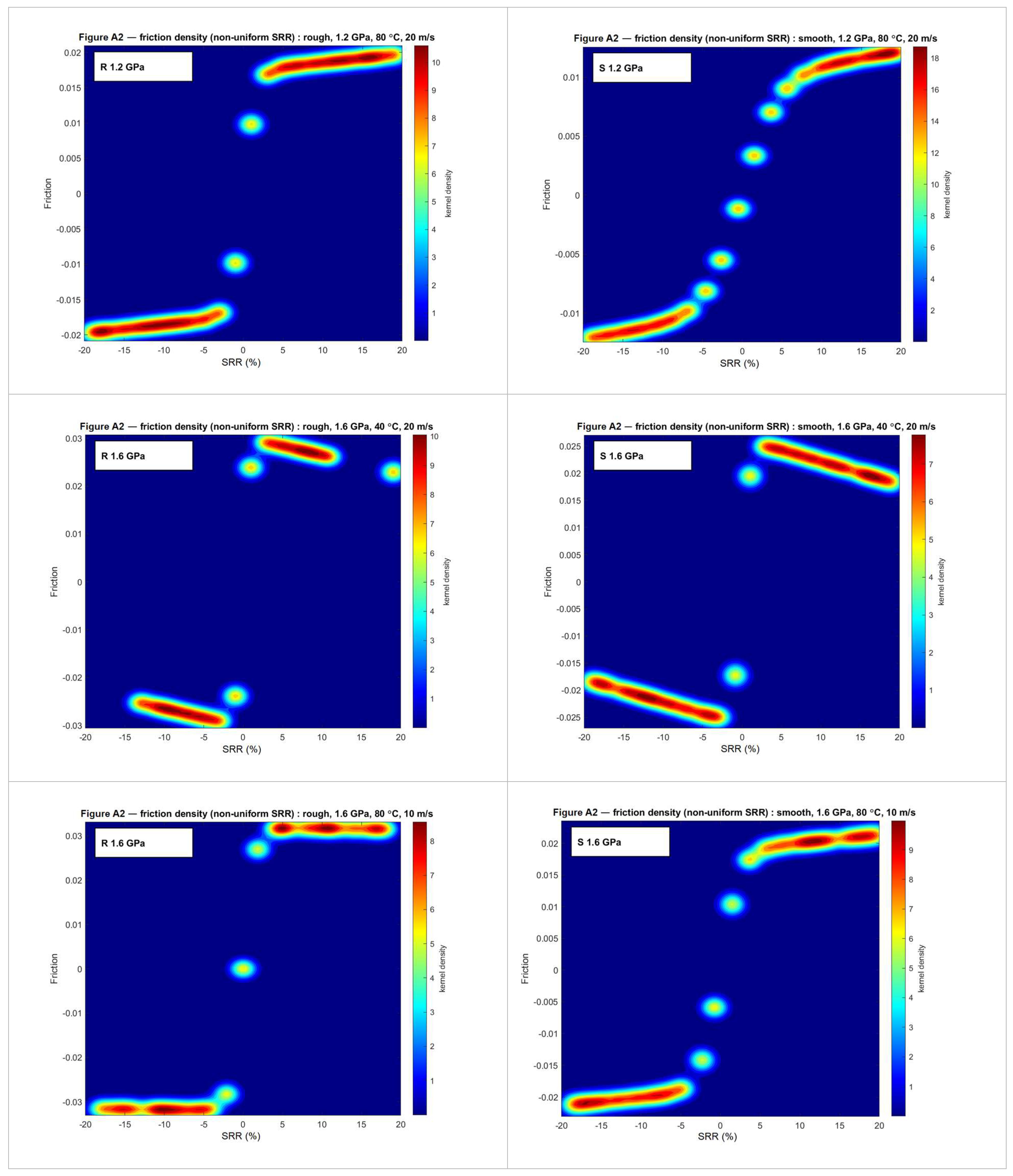
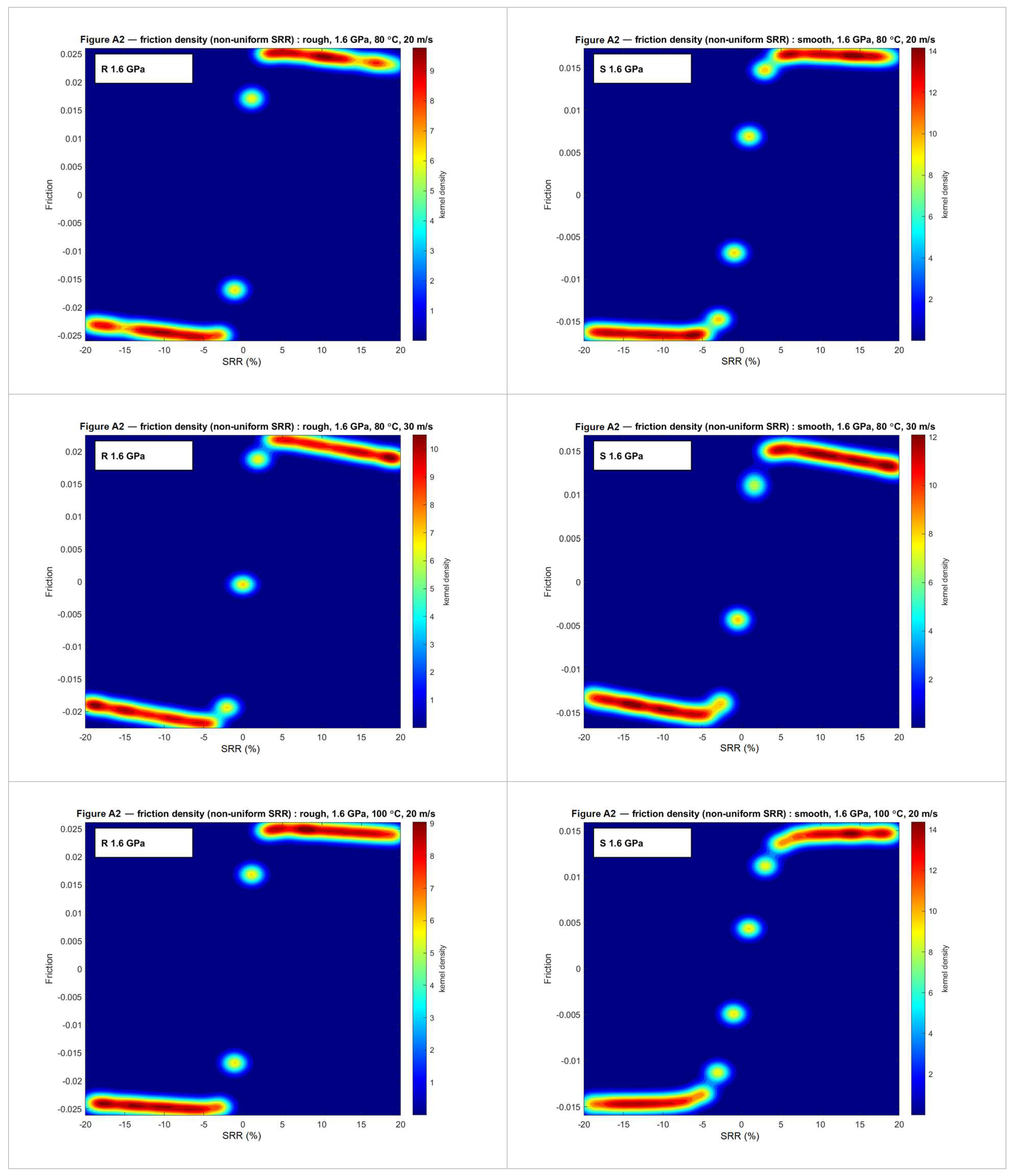
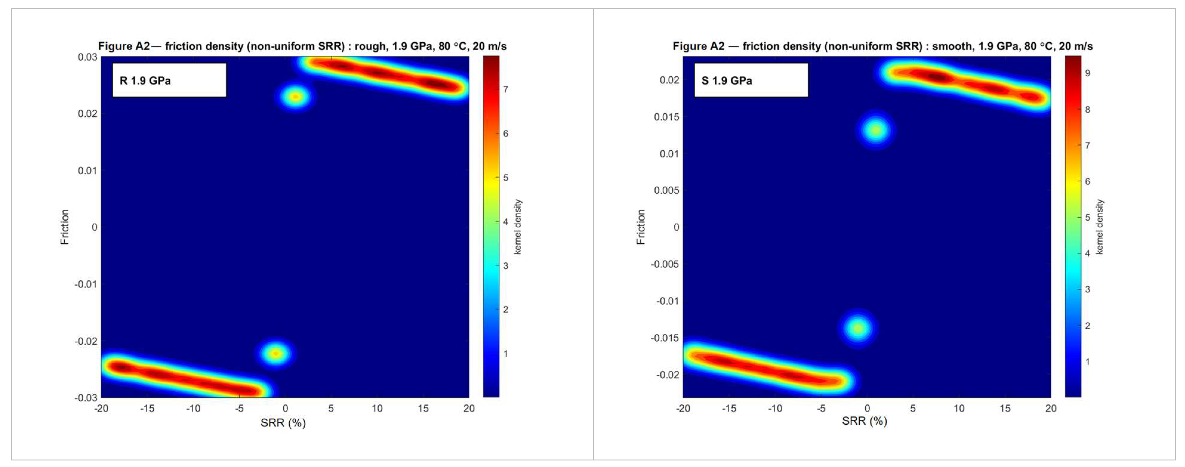
Appendix A.3. Probability Density Plots—Uniform SRR Sampling (Complete Set of Figure 8)
Figure A3.
Probability density of the friction coefficient recomputed at evenly spaced SRR intervals from the bootstrapped parameters for rough and smooth surfaces at each operating condition. High-density regions denote consistent predictions.
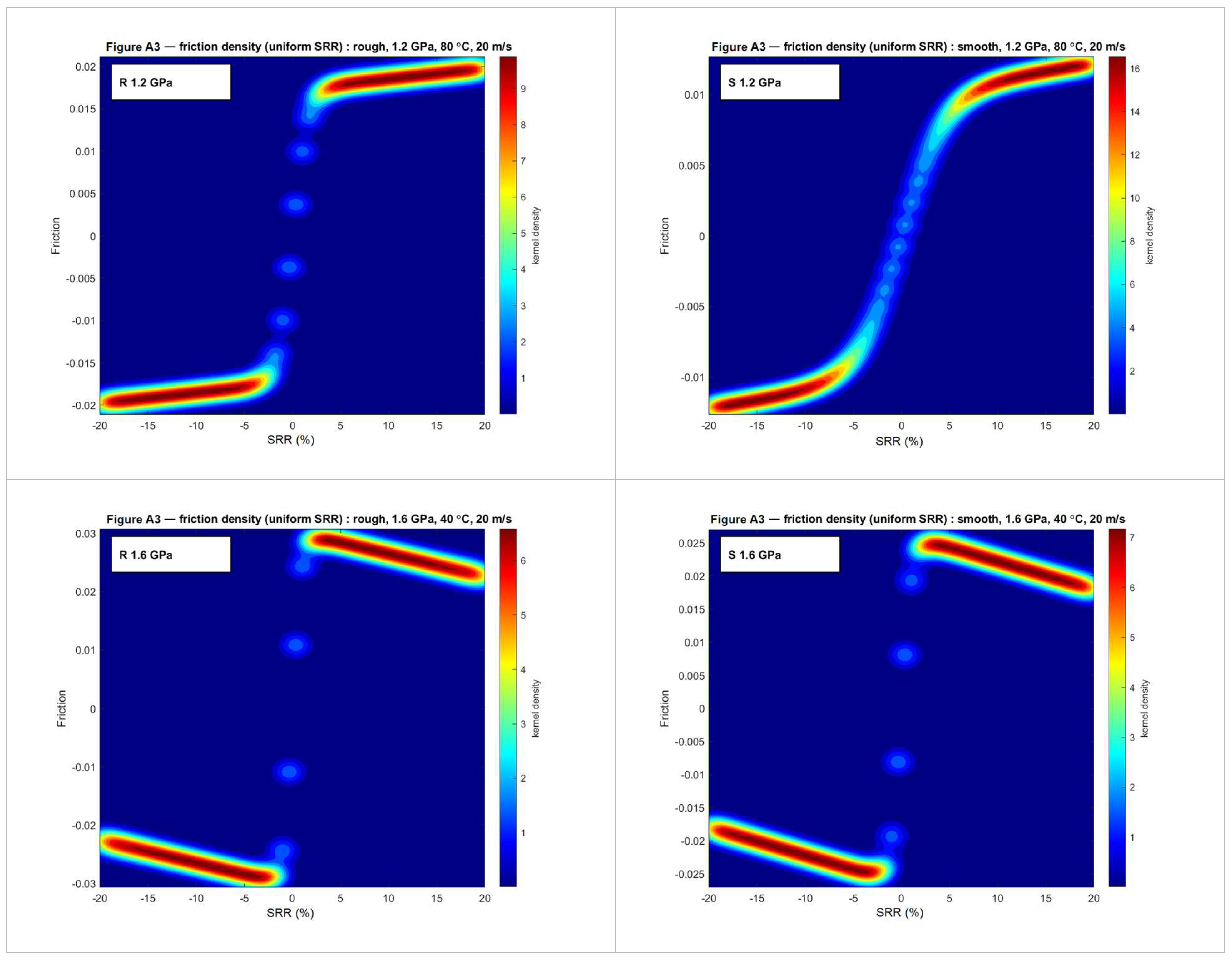
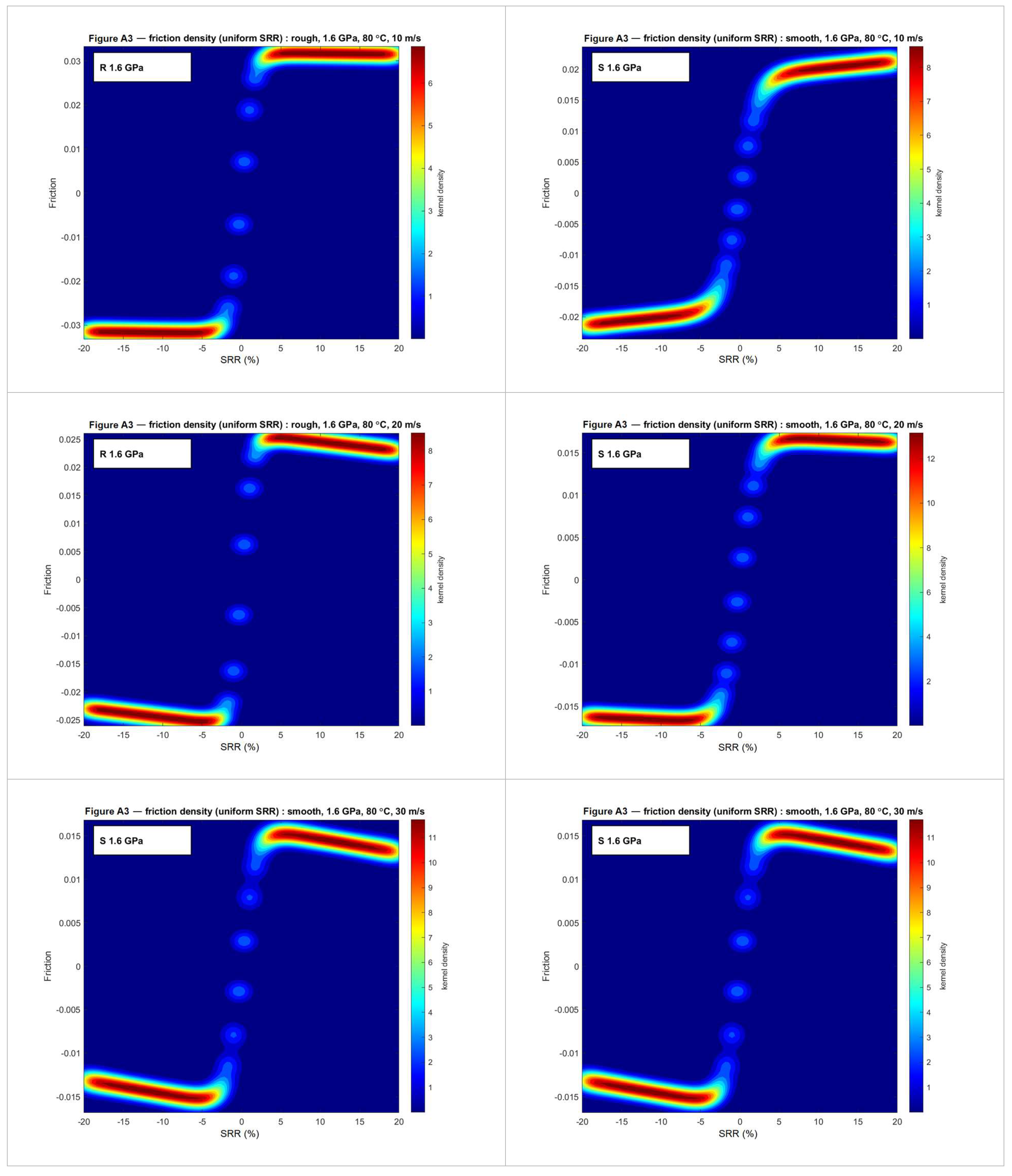
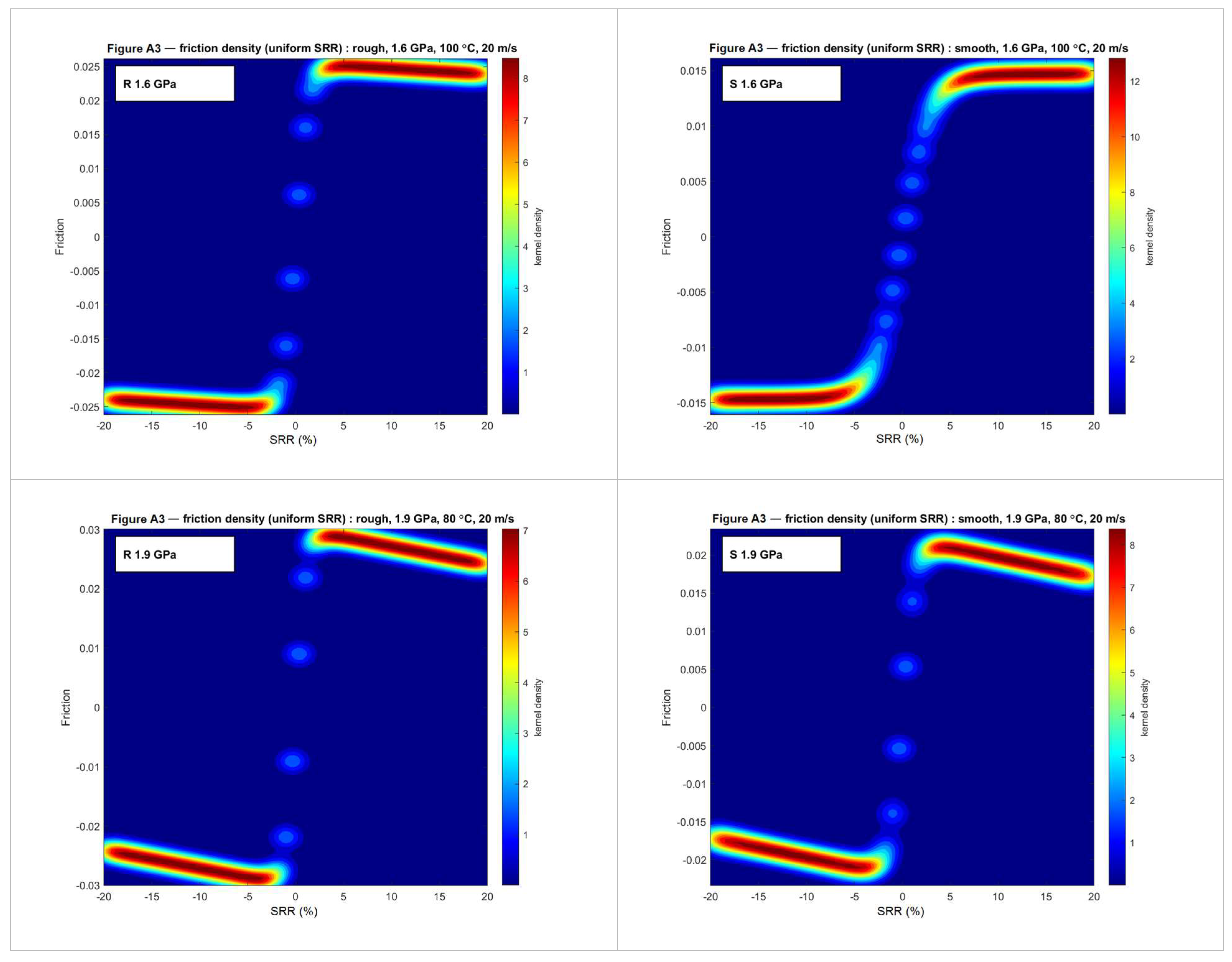
Appendix A.4. Histograms of the Bootstrapped Parameters (Complete Set of Figure 9)
Figure A4.
Histograms of the bootstrapped HAF parameters (columns: ν, a, and h) as a function of the three operating factors of the star design (rows: maximum Hertzian contact pressure, oil temperature, and entrainment speed), comparing rough and smooth surfaces; for each factor, the other two are held at their reference value (1.6 GPa, 80 °C, and 20 m·s−1). Each histogram aggregates 105 bootstrap samples.
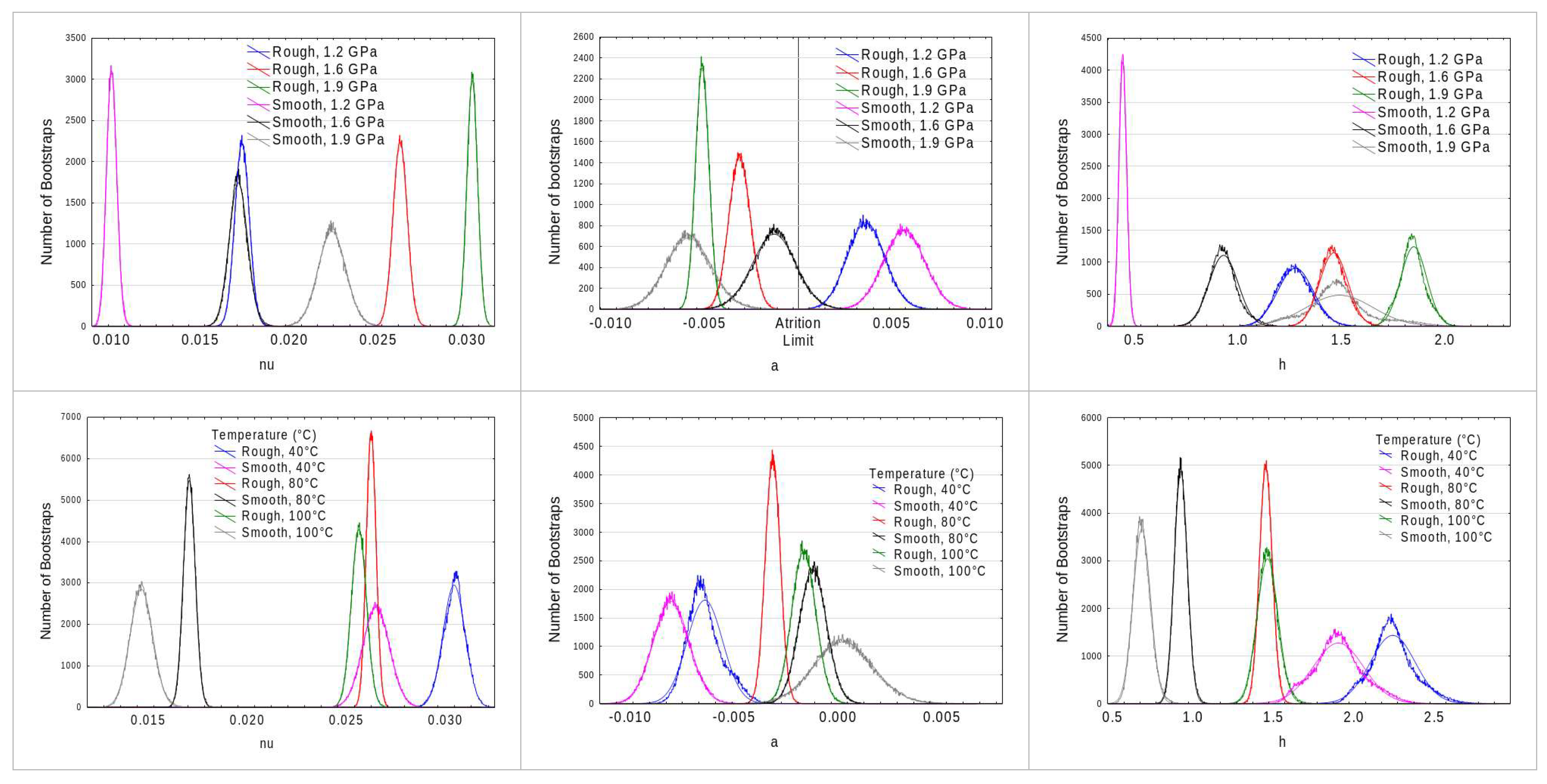
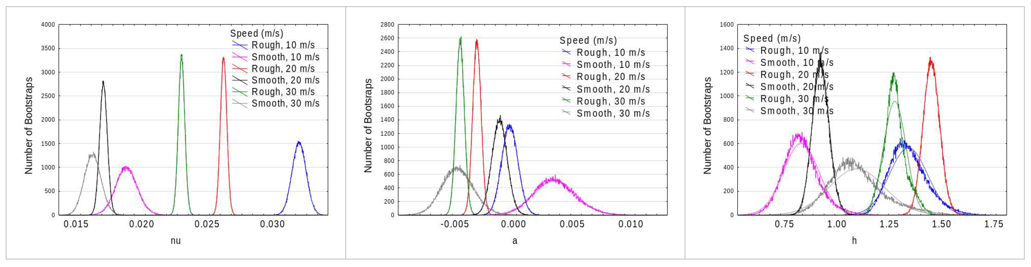
Appendix A.5. Box Plots of the Bootstrapped Parameters (Complete Set of Figure 10)
Figure A5.
Box plots of the bootstrapped HAF parameters (columns: ν, a, and h) as a function of the three operating factors of the star design (rows), comparing rough and smooth surfaces: maximum Hertzian contact pressure (1.2, 1.6, and 1.9 GPa; other factors fixed at 80 °C and 20 m·s−1), oil temperature (40, 80, and 100 °C; fixed at 1.6 GPa and 20 m·s−1) and entrainment speed (10, 20, and 30 m·s−1; fixed at 1.6 GPa and 80 °C). For each factor, the other two are held at their reference value. Boxes show the 5th percentile, 1st quartile, median, 3rd quartile, and 95th percentile of the 105 bootstrap samples.
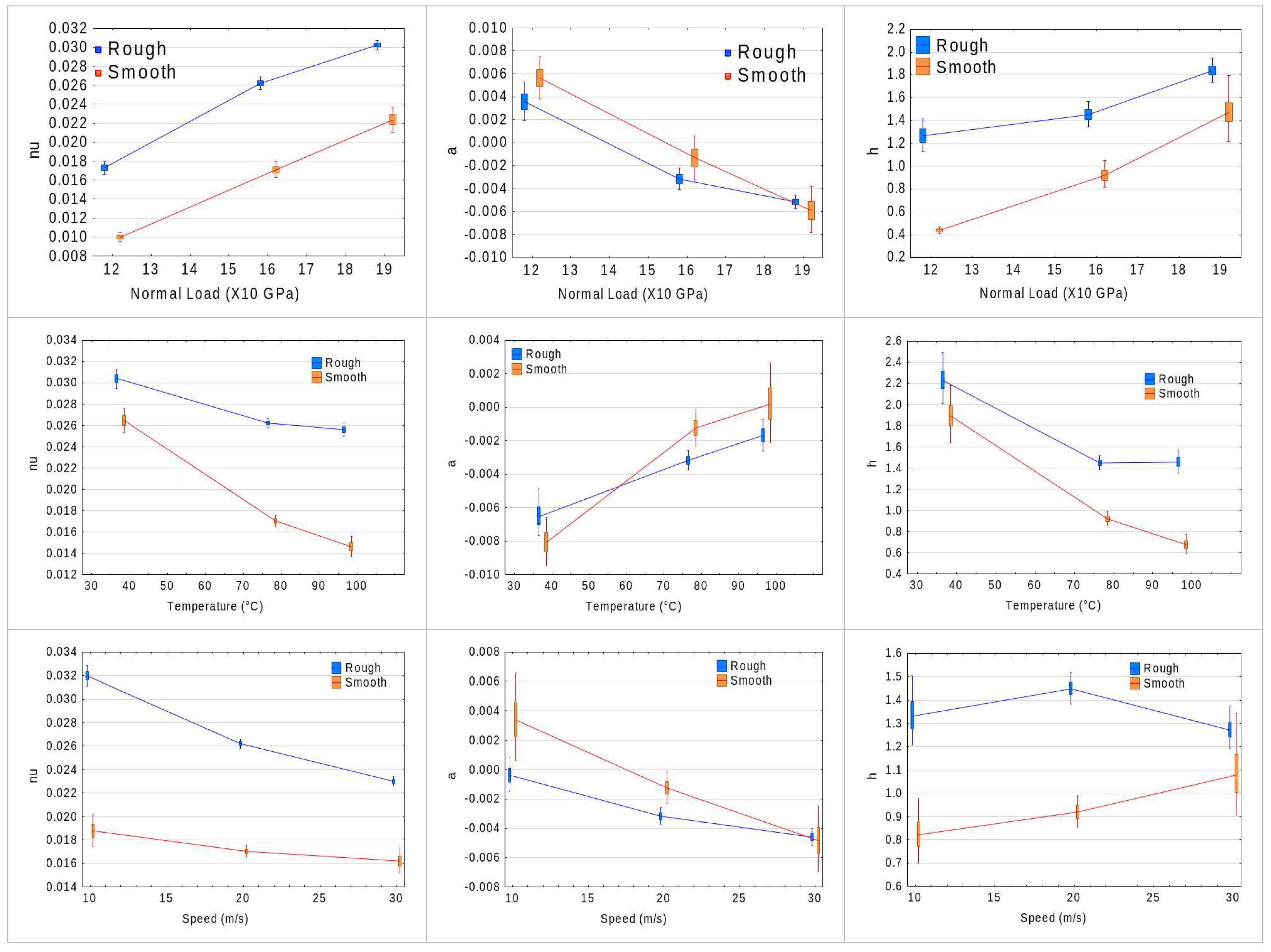
Appendix A.6. Bootstrap Distributions of the Linear-Model Coefficients (Complete Set of Figure 11)
Figure A6.
Complete set of the bootstrap distributions of the linear-model coefficients of h, a, and ν (Section 7.1). Rows = intercept, load, temperature, and speed effects; columns = a, h, and ν.
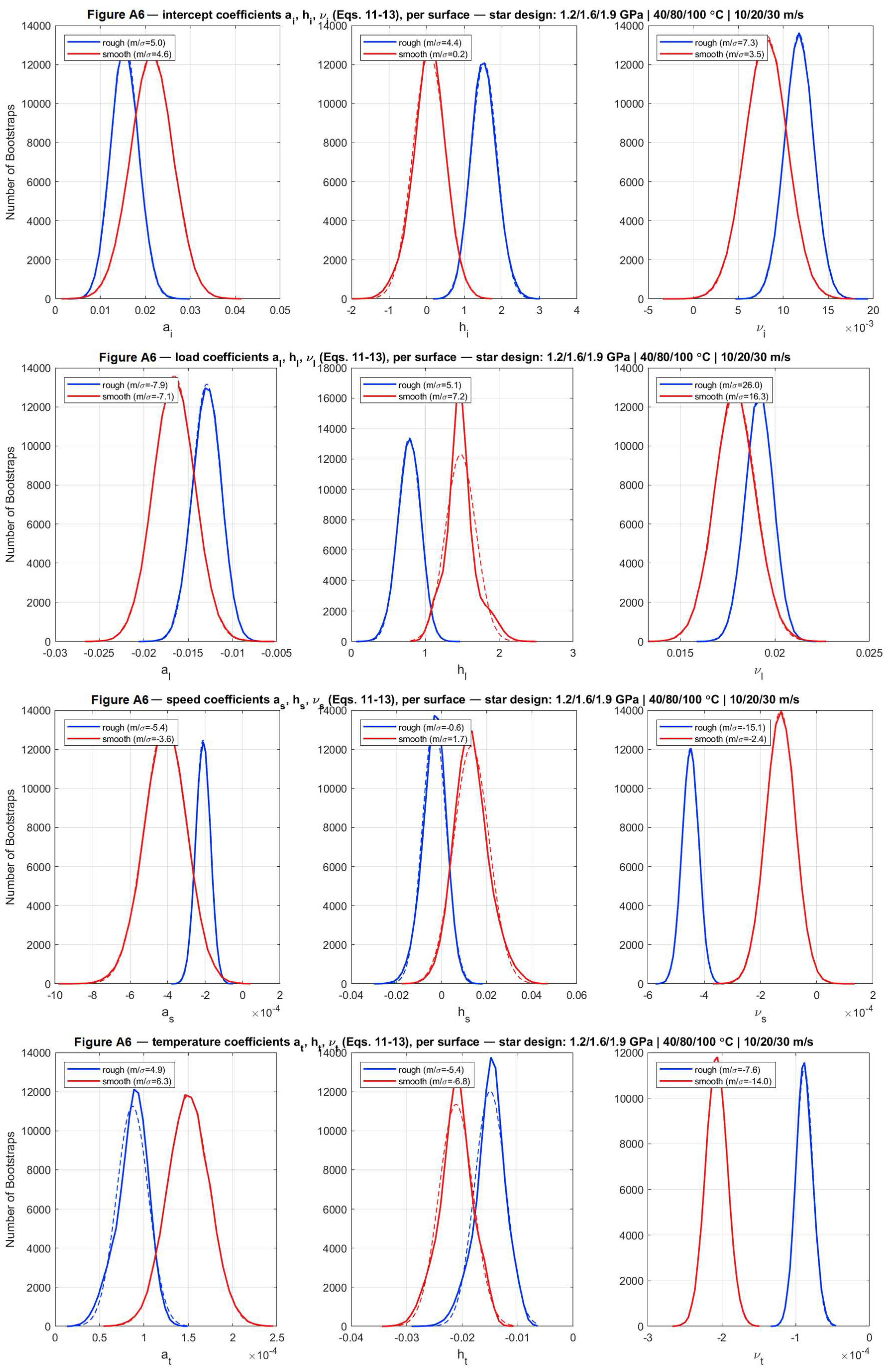
Appendix A.7. Bootstrap Distributions of the Generalized-Model Coefficients (Complete Set of Figure 13)
Figure A7.
Complete set of the bootstrap distributions of the generalized-model coefficients, including roughness (Section 7.2). Rows = a, h, and ν; columns = intercept, load, temperature, speed, and roughness effects, plus the associated R2.
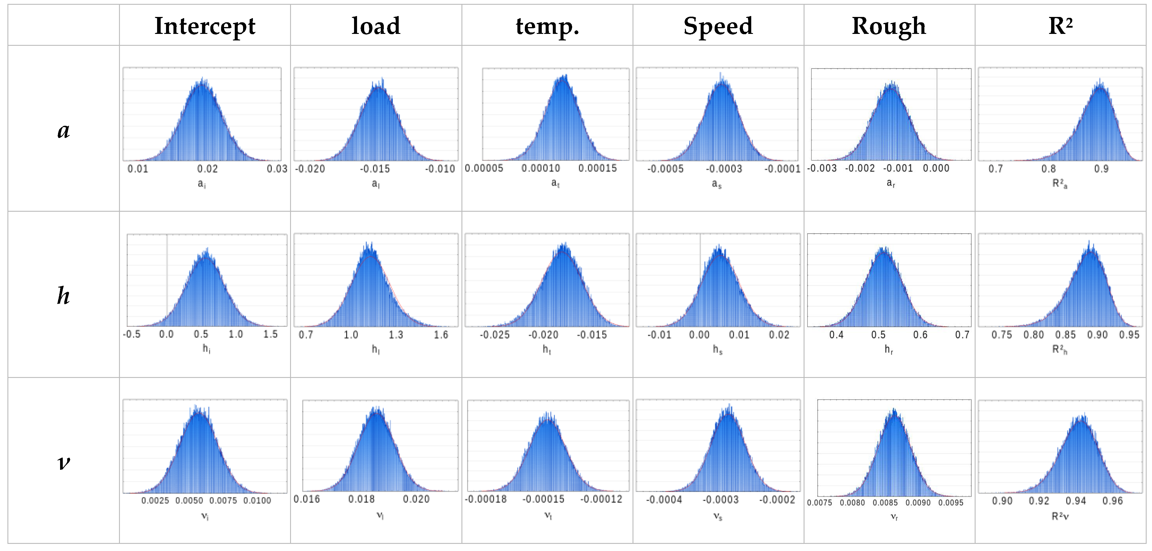
Appendix A.8. Bootstrap Distributions of the Complete-Model Coefficients (Complete Set of Figure 14)
Figure A8.
Complete set of the bootstrap distributions of the fifteen coefficients of the complete nonlinear predictive model (Section 7.3): rows = a, h, and ν; columns = intercept, load, temperature, speed, and roughness effects.
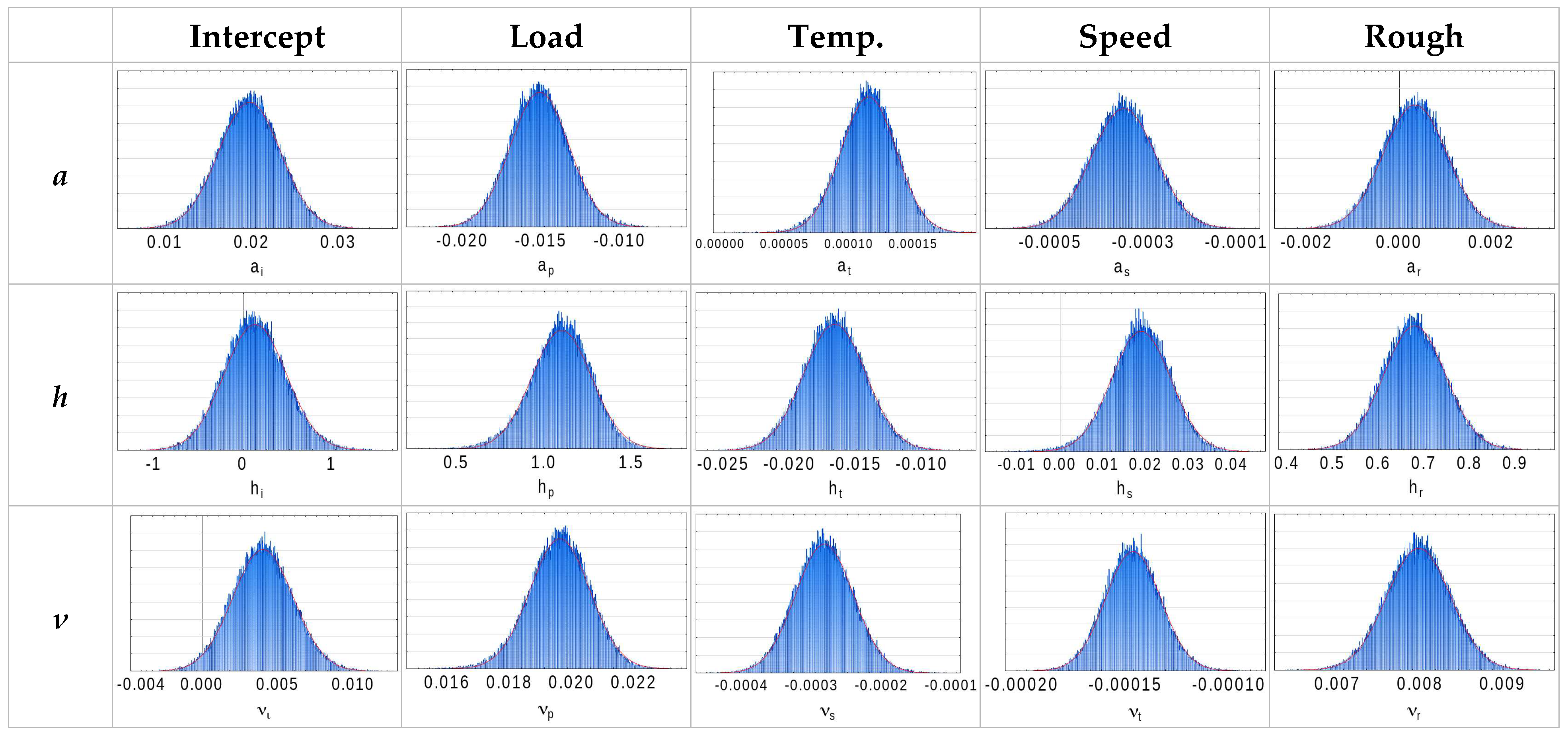
Appendix A.9. Recalculated Friction Curves (Complete Set of Figure 18)
Figure A9.
Experimental friction curves (points) and their reconstruction by the complete model (lines) for the full set of operating conditions (Section 7.3).
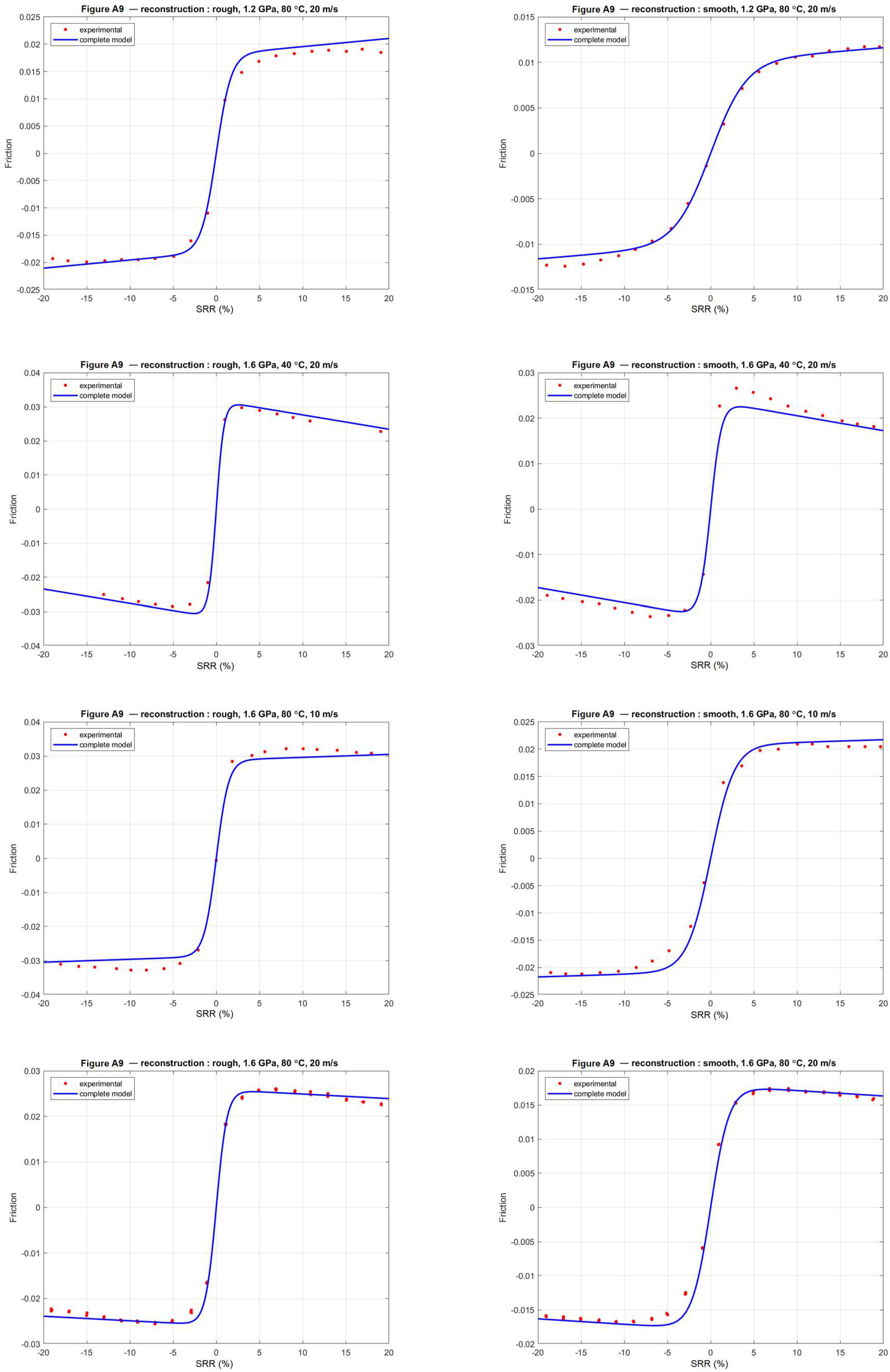
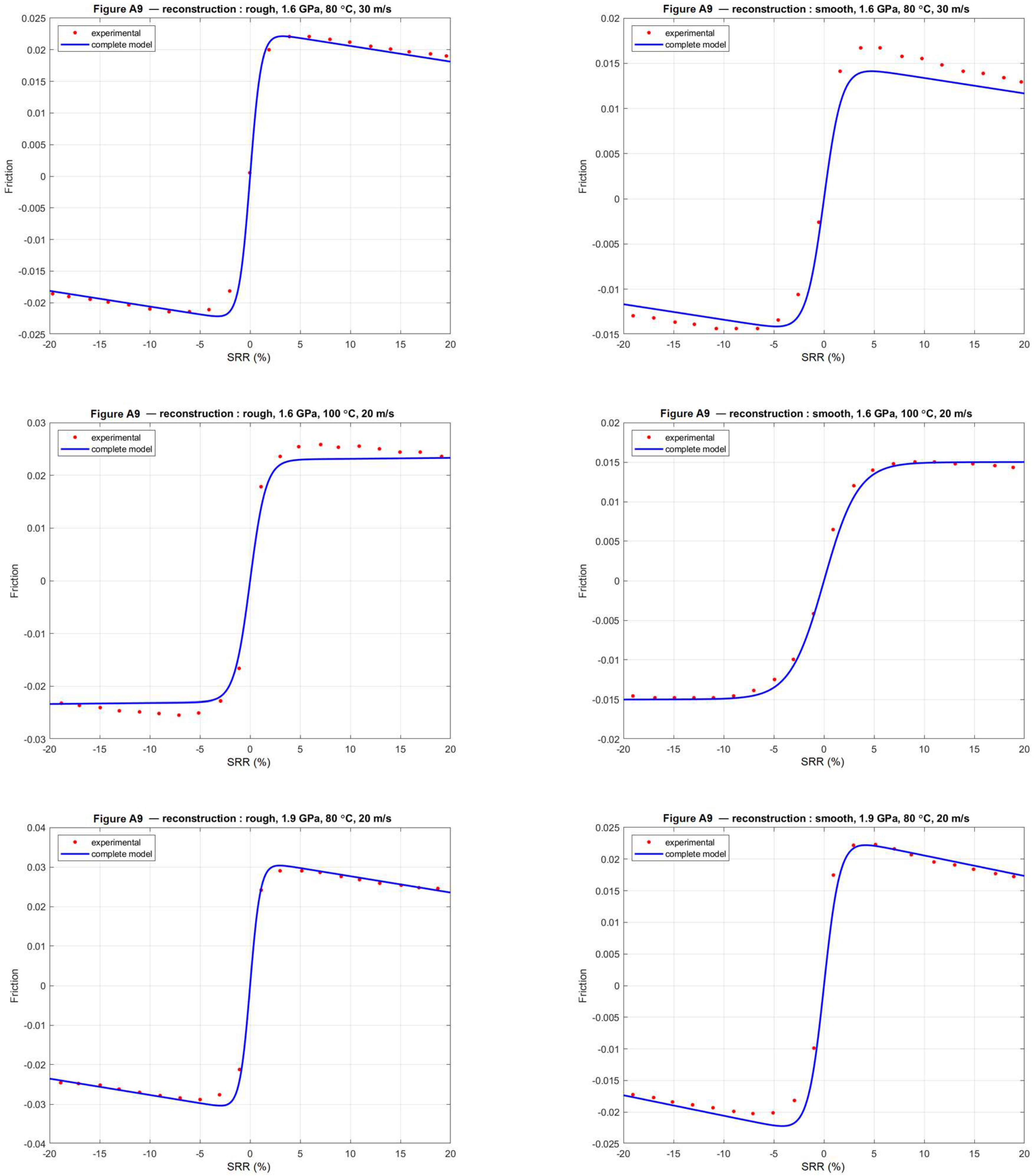
Appendix B. Program and Reproducibility
All results reported in this work were produced by a single, self-contained MATLAB program (HAF_model.m, run under MATLAB R2025b, The MathWorks Inc., Natick, MA, USA) applied to one input file. The program is deliberately compact and toolbox-free so that it can be inspected, rerun, and adapted with minimal effort.
Model and method. Each experimental traction curve is described by the three-parameter HAF form, F(SRR) = 2ν·[1/(1 + exp(−h·SRR)) + a·SRR − 0.5], fitted by nonlinear least squares. The uncertainty of every parameter, and of every quantity derived from it, is obtained by the BIG bootstrap: residuals are resampled, and the model is refitted a large number of times, so that each parameter, each regression coefficient of the linear laws (Equations (19)–(21)), and the complete nonlinear model inherit a full sampling distribution rather than a single value. The significance of the regression coefficients of the linear laws is assessed separately, from the least-squares standard errors on the fourteen operating conditions (Section 7.2).
Input. A single semicolon-separated file, SRR_frot_data.csv, with one row per measurement and the columns rugo, pression, temperature, Vitesse, SRR, and F, respectively, the surface state (rough/smooth), the contact pressure (GPa), the injection temperature (°C), the mean entrainment speed (m/s), the slide-to-roll ratio (%), and the friction coefficient, read from the published curves. The dataset used here comprises the fourteen operating conditions of the star design.
Output. Table 1, Table 2, Table 3 and Table 4 are written to ./HAF_tables/ as CSV files and, in MATLAB, as a formatted HAF_tables.xlsx workbook; all figures are written to ./HAF_figures/PNG/ and ./HAF_figures/BMP/, including both the body figures and the complete per-condition sets of Appendix A.
Options. The main parameters are grouped at the top of the file: nBootCurve (per-curve bootstrap replicates; 103 for a quick run, up to 105 for publication-level standard deviations), nBootComplete (replicates of the fifteen-coefficient complete model; ≈nBootCurve/20 is sufficient) and refitMode (‘local’, fast, or ‘grid’, which reproduces the exhaustive SAS BIG search). Body figure, appendix figure, and spreadsheet outputs can be toggled independently.
Reproducibility. The random number generator is initialized with a fixed seed, so a given configuration yields identical tables and figures on every run and across MATLAB and Octave. To reproduce the results, place HAF_model.m and SRR_frot_data.csv in the same folder and execute the script.
Appendix C. Uncertainty Quantification: Digitization, Validation, and Residual Dependence
The traction curves analyzed in this work were read from the figures published by Quiban et al. [1]. Two reviewers asked how much uncertainty this reading step introduces, and how it propagates to the coefficients of the parametric laws. This appendix addresses both questions. It quantifies the reading step alone: it does not capture a possible systematic distortion of the original figure, nor the experimental uncertainty of the traction measurements themselves, neither of which can be recovered from published curves. The question addressed here is therefore a precise one—given the available documents, what proportion of the reported uncertainty is attributable to digitization?
Appendix C.1. Digitization Protocol
The published figure was rendered from the source PDF at 150 dots per inch, and the panels were digitized with WebPlotDigitizer. For each panel, the two axes were calibrated on their outermost labeled tick marks, −20% and +20% for the slide-to-roll ratio and −0.04 and +0.04 for the friction coefficient, and each experimental marker was digitized individually; only the experimental points, not the continuous model curves shown in the original figure, were digitized. This yields 350 (SRR, F) pairs over the fourteen operating conditions, which is about twenty points per curve. The two curves of the reference condition contain 57 and 59 points because that condition was read once for each of the three sweeps.
Appendix C.2. Estimating Digitization Repeatability
The reference operating point (1.6 GPa, 80 °C, 20 m·s−1) is the common center of the three sweeps of the star design, so it appears in each of the three panels of the published figure and was digitized three times independently. These three readings describe the same physical curve, and any difference between them can only come from the reading operation itself; they therefore provide a direct estimate of repeatability, independently of any modeling assumption.
Because the abscissa of a reading is never exactly reproduced, the points were grouped by proximity in SRR, with a threshold of half a percentage point. This grouping yields twenty groups per surface state: seventeen complete triplets and three pairs on the rough curve, and nineteen triplets and one pair on the smooth curve, with the pairs corresponding to a point missed by one of the three readings. Within each group, the standard deviation of the friction coefficient was computed, and the forty resulting values were pooled by weighting each variance by its degrees of freedom.
The pooled digitization repeatability is 1.6 × 10⁻⁴ in friction-coefficient units, based on 116 readings of 40 repeated points. It is 2.0 × 10⁻⁴ on the rough curves and 1.1 × 10⁻⁴ on the smooth ones, a difference consistent with the fact that the rough curves are denser, intersect one another, and are therefore more difficult to digitize.
Appendix C.3. Propagating the Reading Error
A Monte Carlo simulation was used rather than an analytical propagation, because the HAF model is not linear in its parameters and a linearized propagation would be approximate. Gaussian noise with the standard deviation measured above, taken separately for each surface state, was added to the 350 digitized points; the three HAF parameters were re-estimated for each of the fourteen conditions, and the fifteen coefficients of the parametric laws were then refitted. The operation was repeated one thousand times with a fixed random seed. None of the fourteen thousand nonlinear fits failed, and the mean estimates of the perturbed coefficients reproduce the reported values, which confirms that the noise introduces no bias. The procedure is summarized in Figure A10.
Figure A10.
Procedure used to quantify and propagate the digitization uncertainty, from the triplicate readings of the reference condition to the comparison with the bootstrap dispersion.
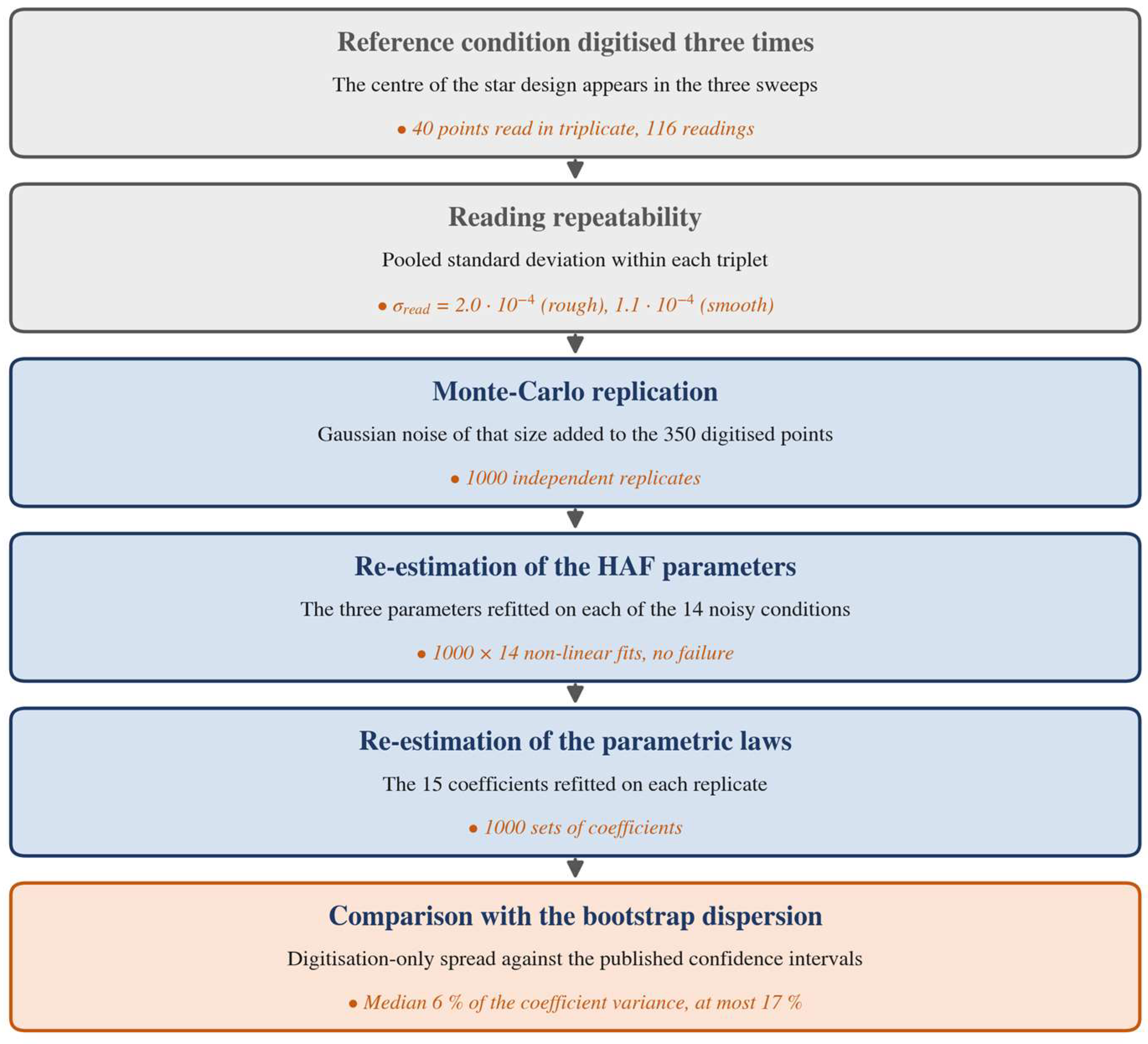
The noise was assumed to be independent from point to point, which is the natural assumption for a digitization error. A systematic distortion of the published figure would instead produce correlated errors and would not be captured by this procedure.
Appendix C.4. Propagation Results
Table A1 compares, for each of the fifteen coefficients, the dispersion produced by digitization alone with the bootstrap dispersion reported in Section 7. The ratio of the two standard deviations lies between 0.17 and 0.41, with a median of 0.25. Since variances accumulate, digitization accounts for a median of 6% of the variance of the coefficients, and for at most 17%, which was reached by the intercept and the load coefficient of the attrition parameter. Figure A11 shows the two distributions superimposed for three representative coefficients, and Figure A12 ranks the fifteen coefficients by the share of variance attributable to reading.
Table A1.
Dispersion of the fifteen coefficients of the parametric laws: contribution of the digitization alone, compared with the bootstrap dispersion reported in Section 7. The variance share is the square of the ratio of the two standard deviations.
Figure A11.
Dispersion of three representative coefficients: the narrow histogram is the spread produced by digitization alone, and the broad curve is the bootstrap dispersion reported in Section 7. The dashed line marks the published estimate. The dashed vertical line marks the coefficient value estimated on the original data.
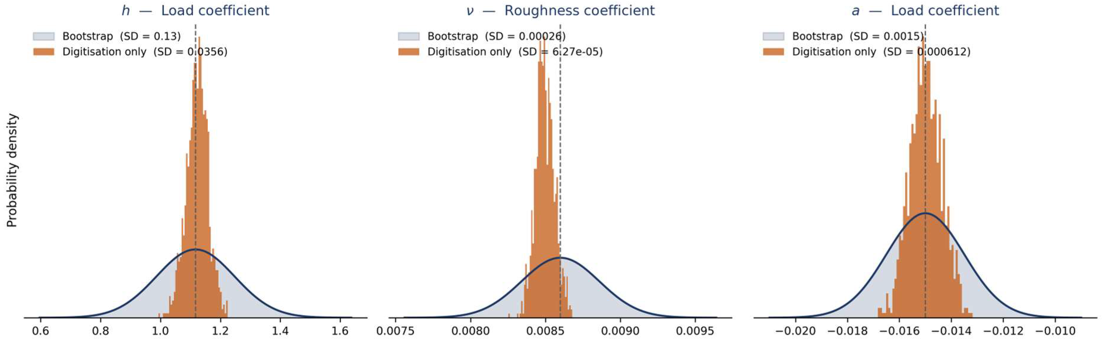
Figure A12.
Share of the variance of each of the fifteen coefficients attributable to the digitization of the published curves. Two coefficients exceed 10%, both belonging to the attrition parameter. The dashed vertical line marks the median share over the fifteen coefficients.
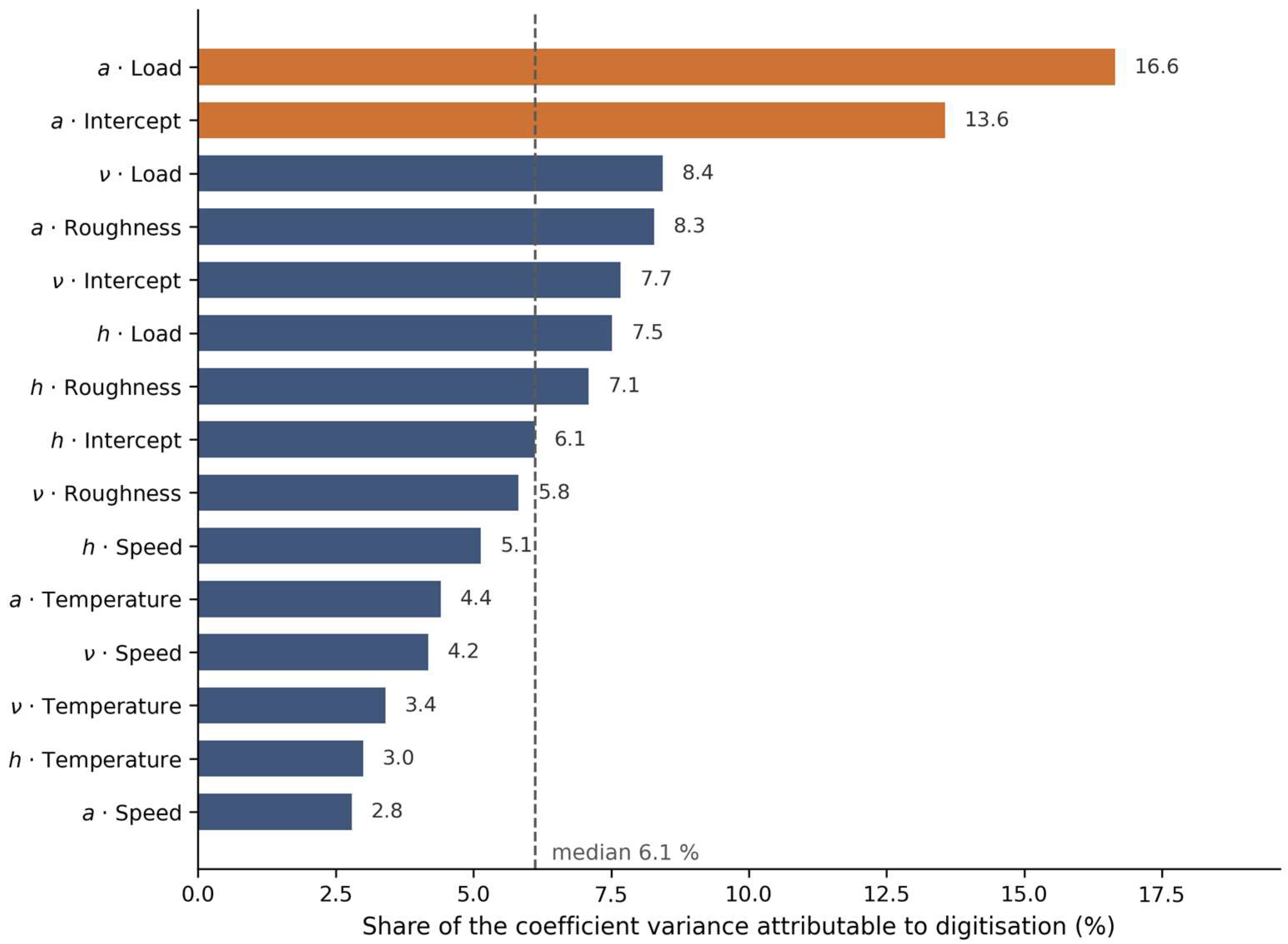
These figures show that reading the published curves is a measurable but secondary contributor to the uncertainty reported in this work: even perfect digitization would narrow the confidence intervals by only a few percent, with the remainder arising from the dispersion of the data about the model and from the limited number of operating conditions.
Appendix C.5. Leave-One-Condition-Out Validation: Principle
This section details the validation reported in Section 7.4. It is organized in three parts: the validation procedure itself, the construction of the prediction intervals, and the computation of their coverage.
Appendix C.6. Validation Procedure
The fourteen operating conditions are treated in turn. For the condition under test, everything that belongs to it is set aside: its digitized points and the parameter triplet fitted to them. The three parametric laws are then re-estimated by least squares on the thirteen retained triplets only, giving a new set of coefficients for ν, h, and a. These laws are applied to the operating variables of the excluded condition—its contact pressure, injection temperature, mean speed, and surface state—which yields its three predicted parameters. Because the excluded curve contributed neither points nor parameters to this estimation, the prediction is genuinely out-of-sample.
A standard deviation of prediction is then computed for each parameter, as described in Appendix C.7, and two thousand parameter triplets are drawn around the predicted values. Each triplet, substituted into the HAF equation, produces one complete friction curve, so that at every measured value of the slide-to-roll ratio, two thousand predicted friction values are available; their 2.5th and 97.5th percentiles define the 95% prediction interval at that abscissa. The predicted curve is finally compared with the measured one: the errors give the root mean square error, the mean absolute error, and the largest absolute error for that condition, and the number of measured points falling inside their interval gives the coverage. The operation is repeated for the fourteen conditions, and the errors are pooled over the 350 predicted points. The procedure is summarized in Figure A13.
Figure A13.
Leave-one-condition-out validation procedure. Each of the fourteen conditions is removed in turn; the parametric laws are re-estimated on the thirteen others and used to predict the excluded curve, which contributed nothing to the estimation. The dashed arrow marks the return of the loop, the procedure being repeated for each of the fourteen conditions in turn.
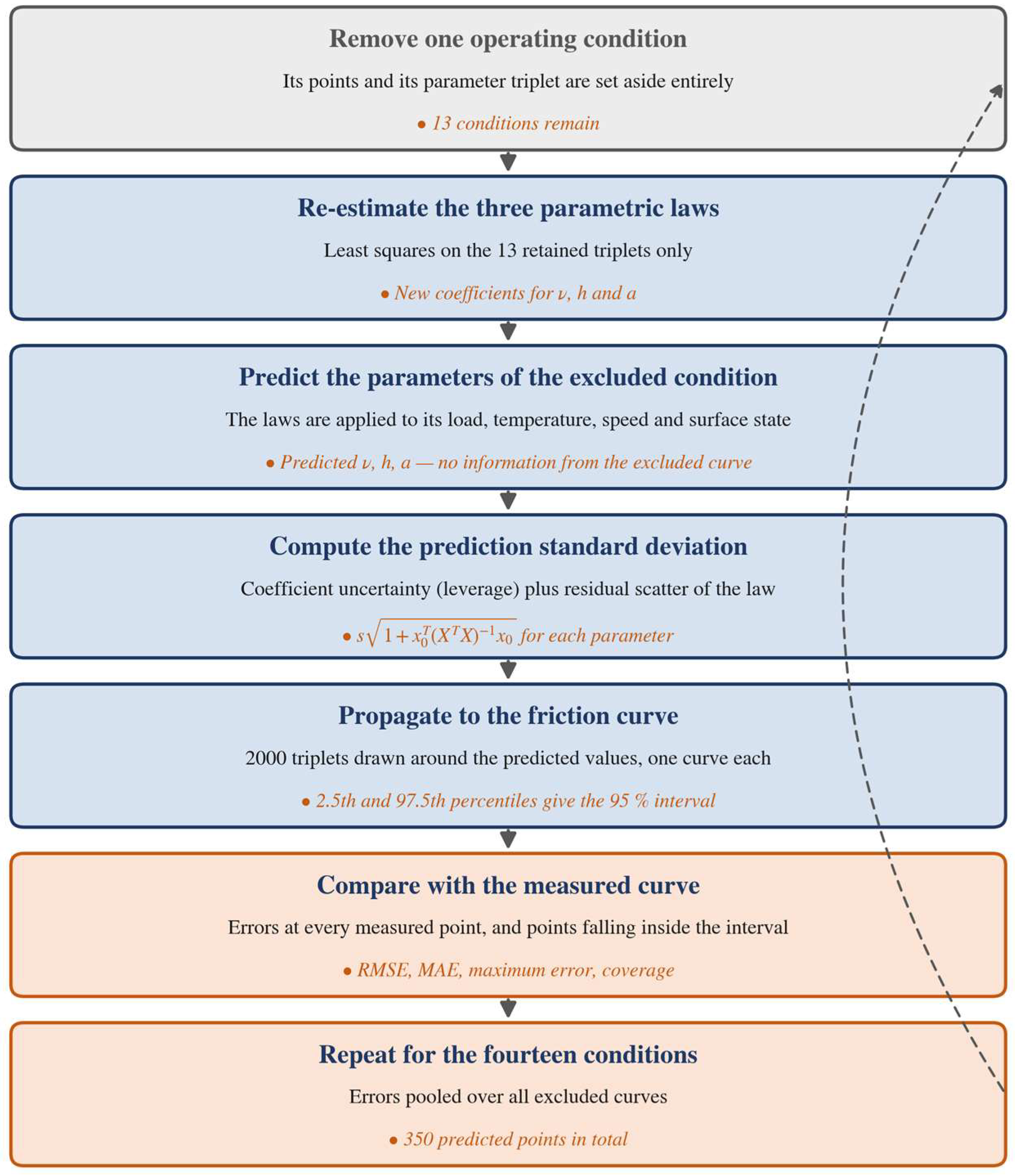
Appendix C.7. Construction of the Prediction Intervals
Predicting a parameter for a condition that took no part in the estimation involves two independent sources of error, which must be combined.
The first is the uncertainty of the coefficients of the parametric law, estimated from thirteen conditions only. For a condition described by the vector x0 = (1, load, temperature, speed, and roughness), and with X being the design matrix of the thirteen retained conditions, this contributes a variance s2·x0ᵀ (XᵀX)−1 x0. The quadratic form is the leverage of the predicted condition: it is small at the center of the experimental domain and grows toward its edges. This is why the conditions lying at the ends of the star design are predicted less precisely than the central ones, as Figure 19 shows.
The second is the residual scatter of the parameters about the law. The thirteen retained triplets do not lie exactly on the fitted plane, and the excluded condition will not either; even with perfectly known coefficients, its parameters could not be predicted more accurately than this scatter. It is estimated by s2 = RSS/(13 − 5), the residual sum of squares of the law divided by its eight degrees of freedom, under the usual assumption that the scatter is the same at every condition.
Because the two sources are independent, their variances are added together, so that the standard deviation of the prediction of each parameter is s√(1 + x0ᵀ (XᵀX)−1 x0). The first term inside the bracket is the scatter of the new point about the law and does not depend on where the prediction is made; the second is the uncertainty regarding the position of the law itself and does depend on where the prediction is made.
Appendix C.8. Coverage of the Prediction Intervals
A prediction interval is a claim, and the coverage tests it: if the intervals are well calibrated, about 95% of measured points should fall inside their own 95% interval. The test is meaningful only because no point contributed to the construction of its own interval. Over the fourteen excluded conditions, 96% of the 350 measured points fall inside their interval, against a nominal 95%, so the uncertainty attached to a prediction is realistic and, if anything, slightly conservative. For comparison, intervals built on the bootstrap standard deviations of the coefficients alone give 98%.
Appendix C.9. Dependence of the Residuals Along a Curve
The residual bootstrap used in Section 5 assumes that the residuals of a curve are exchangeable, that is, that they can be permuted without loss. This assumption deserves examination, because the points of a traction curve are not independent measurements: they were read one after another along the same published curve, so that two neighboring points share the same local model discrepancy.
Appendix C.10. Diagnosis of the Dependence
The residuals were examined curve by curve as a function of the slide-to-roll ratio (Figure A14). The dependence is real, and it is substantial: the lag-one autocorrelation averages 0.51 over the fourteen conditions, reaches 0.85, and exceeds 0.3 for eleven of them; the mean Durbin–Watson statistic is 0.70, compared with 2.0 for independent residuals; and a runs test on the sign of the residuals rejects independence for nine curves. The dependence is strongest on the smooth curves and essentially absent on three of the rough curves.
The residual plots also reveal something the autocorrelation alone would not show. On rough discs, the residuals are scattered without any marked structure, whereas on smooth discs, they follow a systematic pattern: a positive hump centered on zero sliding, indicating that the model slightly underestimates friction just after the transition. Averaged over the seven curves of each surface state, the residual for |SRR| < 3% is +0.0018 on smooth discs and +0.0008 on rough discs, compared with less than 0.0001 beyond |SRR| = 8%. A one-sample test on the fourteen curve averages gives p = 0.004 for the smooth surfaces and p = 0.025 for the rough surfaces, so this offset is systematic rather than accidental. Its largest value, 0.0043, occurs on the smooth curve at 1.9 GPa and a slide-to-roll ratio of about 1%.
Part of the dependence along a curve therefore arises not from the reading of the published figure but from a small mismatch of shape: the real transition at zero sliding is slightly sharper than the logistic form can render. The effect is twice as large under full-film lubrication, where the transition is governed by the rheology of the lubricant alone, without the gradual contribution of the asperities. The amplitude nevertheless remains modest, at about a tenth of the plateau friction level.
Figure A14.
Residuals of the HAF fit against the slide-to-roll ratio, for the seven rough conditions (top) and the seven smooth conditions (bottom). On smooth discs, a systematic positive hump appears around zero sliding.
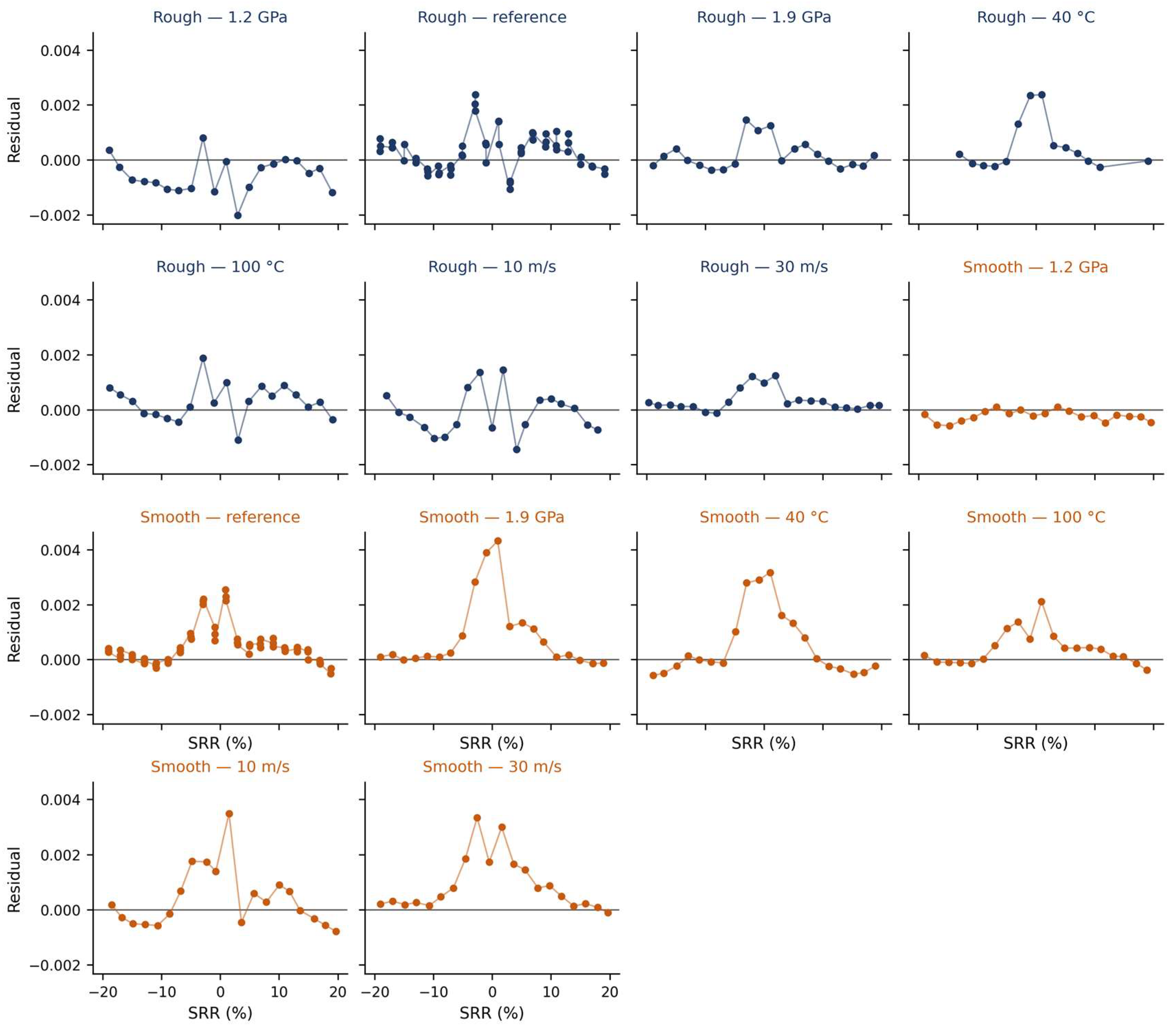
Appendix C.11. Block Resampling
To assess the consequences of this dependence, the resampling was repeated on blocks of consecutive residuals rather than on individual ones. In this moving-block scheme, segments of L successive residuals are drawn with replacement and concatenated until the length of the original series is recovered, so that the correlation structure inside a block is preserved. Block lengths of one, three, five, and seven were used, with L = 1 reproducing the ordinary residual bootstrap, with 4000 replicates each (Figure A15).
Figure A15.
(Left) standard deviation of each HAF parameter obtained by moving-block resampling, relative to its value for L = 1, as a function of the block length in number of consecutive residuals; the line is the median over the fourteen conditions and the band is the interquartile range. (Right) lag-one autocorrelation of the residuals for each of the fourteen operating conditions, with each bar labeled by its contact pressure, injection temperature, and mean speed, and colored by surface state.
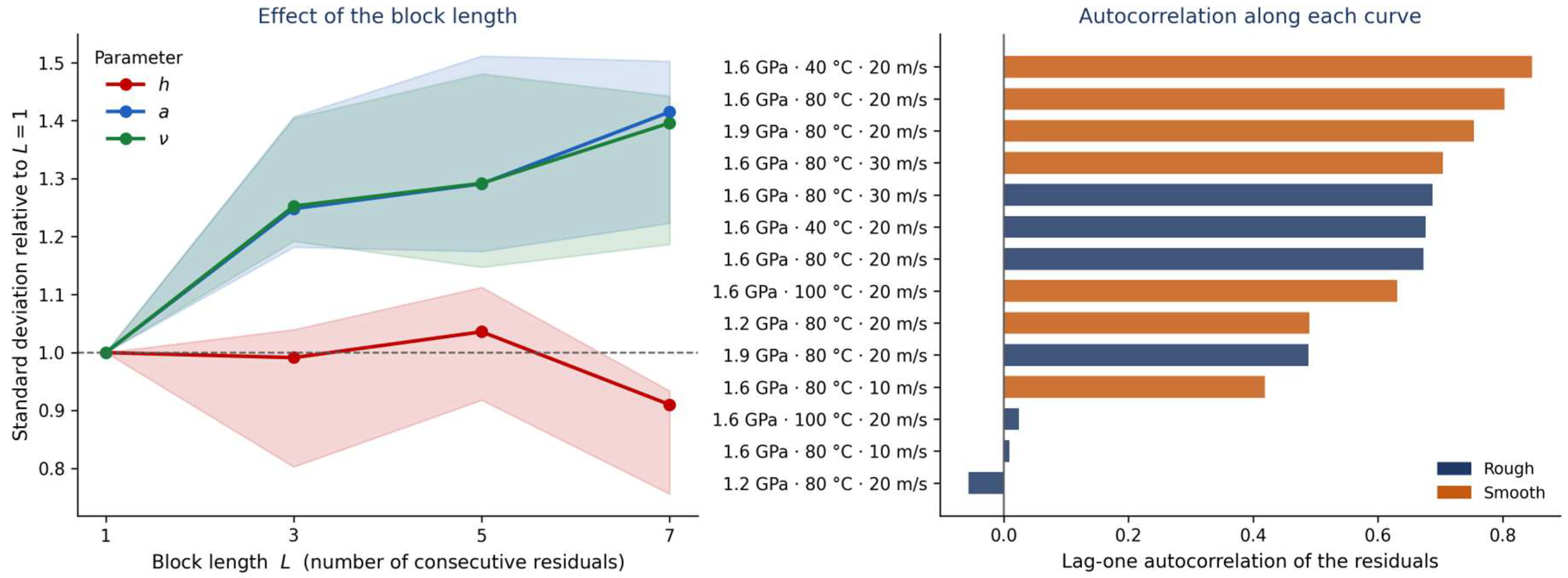
The standard deviations of the parameters widen by about 20% on average, and the effect saturates from L = 3 onward, which indicates that the dependence extends over only two or three consecutive points. The effect, however, differs markedly among parameters, and this inequality is informative. It is systematic for a and ν, whose standard deviations grow by 20 to 40%, because these two parameters are determined by the plateaus, that is, by long stretches of the curve over which neighboring points share the same departure from the model. It is absent for h, which is fixed by the transition around zero sliding, over a handful of points where the correlation has little scope to affect the estimate.
Appendix C.12. Consequences of the Dependence
The correction matters for the parameter distributions of Section 5 and Section 6, which should be read as about 20% wider for a and ν. It does not affect the inference in Section 7. As shown in that section, the uncertainty of the coefficients of the parametric laws is not governed by the precision of each individual triplet but by the scatter of the fourteen triplets about the fitted plane, and that scatter is measured directly by the least-squares residuals of the laws, without relying on the bootstrap. Repeating the block resampling and refitting the laws on each replicate changes the standard errors of the fifteen coefficients by less than the width of the last digit reported in Table 4. None of the conclusions of this work therefore depends on the exchangeability assumption.
References
- Quiban, R.; Grenet de Bechillon, N.; Touret, T.; Navet, P.; Diab, Y.; Cavoret, J.; Ville, F.; Changenet, C. On the interest of a semi-empirical model for the tooth friction coefficient in gear transmissions. Proc. Inst. Mech. Eng. Part J J. Eng. Tribol. 2021, 235, 2654–2663. [Google Scholar] [CrossRef] [Scilit]
- Britton, R.D.; Elcoate, C.D.; Alanou, M.P.; Evans, H.P.; Snidle, R.W. Effect of surface finish on gear tooth friction. J. Tribol. 2000, 122, 354–360. [Google Scholar] [CrossRef] [Scilit]
- Akbarzadeh, S.; Khonsari, M.M. Performance of spur gears considering surface roughness and shear-thinning lubricant. J. Tribol. 2008, 130, 021503. [Google Scholar] [CrossRef] [Scilit]
- Zhmud, B.; Najjari, M.; Brodmann, B. The effects of the lubricant properties and surface finish characteristics on the tribology of high-speed gears for EV transmissions. Lubricants 2024, 12, 112. [Google Scholar] [CrossRef] [Scilit]
- Yan, S.; Kong, Z.; Liu, H.; Zhang, L.; Hu, X.; Hou, Y. Power loss evaluation of an E-axle gearbox considering the influence of gear oil factors. Lubricants 2024, 12, 11. [Google Scholar] [CrossRef] [Scilit]
- Paturi, U.M.R.; Palakurthy, S.T.; Reddy, N.S. The role of machine learning in tribology: A systematic review. Arch. Comput. Methods Eng. 2023, 30, 1345–1397. [Google Scholar] [CrossRef] [Scilit]
- Marian, M.; Tremmel, S. Recent advances in machine learning in tribology. Lubricants 2024, 12, 168. [Google Scholar] [CrossRef] [Scilit]
- Bigerelle, M.; Lemesle, J.; Chevallier, E.; Diab, Y.; Touret, T.; Changenet, C.; Ville, F. A phenomenological model with bootstrap-based uncertainty estimation for friction coefficient prediction in gear transmissions. Surfaces 2026, 9, 81. [Google Scholar] [CrossRef] [Scilit]
- Diab, Y.; Ville, F.; Velex, P. Prediction of power losses due to tooth friction in gears. Tribol. Trans. 2006, 49, 260–270. [Google Scholar] [CrossRef] [Scilit]
- Liu, L.; Kong, R.; Chen, Z. Prediction of mechanical efficiency of spur gear pairs based on tribo-dynamics model of multi-tooth meshing. Proc. Inst. Mech. Eng. Part J J. Eng. Tribol. 2024, 238, 880–893. [Google Scholar] [CrossRef] [Scilit]
- Diab, Y.; Touret, T.; Ville, F.; Changenet, C. Tooth friction in spur gear transmission: From local to mean tooth friction loss. Proc. Inst. Mech. Eng. Part J J. Eng. Tribol. 2024, 238, 1583–1592. [Google Scholar] [CrossRef] [Scilit]
- Bair, S.; Habchi, W. Quantitative elastohydrodynamic lubrication—Seventeen years in. ASME J. Tribol. 2024, 146, 080801. [Google Scholar] [CrossRef] [Scilit]
- Bair, S. The high-pressure rheology of gear oils. Proc. Inst. Mech. Eng. Part J J. Eng. Tribol. 2025, 240, 641–650. [Google Scholar] [CrossRef] [Scilit]
- Isaac, G.; Changenet, C.; Ville, F.; Cavoret, J.; Becquerelle, S. Thermal Analysis of Twin-Disc Machine for Traction Tests and Scuffing Experiments. Proc. Inst. Mech. Eng. Part J J. Eng. Tribol. 2018, 232, 1548–1560. [Google Scholar] [CrossRef] [Scilit]
- Ville, F.; Nélias, D.; Tourlonias, G.; Flamand, L.; Sainsot, P. On the two-disc machine: A polyvalent and powerful tool to study fundamental and industrial problems related to elastohydrodynamic lubrication. Tribol. Ser. 2001, 39, 393–402. [Google Scholar] [CrossRef] [Scilit]
- Efron, B.; Tibshirani, R.J. An Introduction to the Bootstrap; Chapman & Hall: New York, NY, USA, 1993. [Google Scholar]
- Olver, A.V.; Spikes, H.A. Prediction of traction in elastohydrodynamic lubrication. Proc. Inst. Mech. Eng. Part J J. Eng. Tribol. 1998, 212, 321–346. [Google Scholar] [CrossRef] [Scilit]
- Xu, H.; Kahraman, A.; Anderson, N.E.; Maddock, D.G. Prediction of mechanical efficiency of parallel-axis gear pairs. J. Mech. Des. 2007, 129, 58–68. [Google Scholar] [CrossRef] [Scilit]
- Arana, A.; Larrañaga, J.; Ulacia, I. Partial EHL friction coefficient model to predict power losses in cylindrical gears. Proc. Inst. Mech. Eng. Part J J. Eng. Tribol. 2019, 233, 303–316. [Google Scholar] [CrossRef] [Scilit]
- Benedict, G.H.; Kelley, B.W. Instantaneous coefficients of gear tooth friction. ASLE Trans. 1961, 4, 59–70. [Google Scholar] [CrossRef] [Scilit]
- Kelley, B.W.; Lemanski, A.J. Lubrication of involute gearing. Proc. Inst. Mech. Eng. 1967, 182, 173–184. [Google Scholar] [CrossRef] [Scilit]
- Fernandes, C.M.C.G.; Martins, R.C.; Seabra, J.H.O. Coefficient of friction equation for gears based on a modified Hersey parameter. Tribol. Int. 2016, 101, 204–217. [Google Scholar] [CrossRef] [Scilit]
- Johnson, K.L.; Tevaarwerk, J.L. Shear behavior of elastohydrodynamic oil films. Proc. R. Soc. Lond. Ser. A Math. Phys. Sci. 1977, 356, 215–236. [Google Scholar] [CrossRef] [Scilit]
- Bair, S.; Habchi, W. Rheology extracted from traction curves: Is there enough information? ASME J. Tribol. 2026, 148, 081101. [Google Scholar] [CrossRef] [Scilit]
- Bair, S.; Habchi, W. Elastohydrodynamic lubrication traction coefficient is not a property of the liquid alone. ASME J. Tribol. 2025, 147, 044501. [Google Scholar] [CrossRef] [Scilit]
- Transtrum, M.K.; Machta, B.B.; Sethna, J.P. Geometry of nonlinear least squares with applications to sloppy models and optimization. Phys. Rev. E 2011, 83, 036701. [Google Scholar] [CrossRef] [Scilit]
- Gutenkunst, R.N.; Waterfall, J.J.; Casey, F.P.; Brown, K.S.; Myers, C.R.; Sethna, J.P. Universally sloppy parameter sensitivities in systems biology models. PLoS Comput. Biol. 2007, 3, e189. [Google Scholar] [CrossRef] [Scilit]
- Cordier, M.; Diab, Y.; Cavoret, J.; Majdoub, F.; Changenet, C.; Ville, F. An experimental study on the impact of roughness orientation on the friction coefficient in EHL contact. Lubricants 2025, 13, 340. [Google Scholar] [CrossRef] [Scilit]
- Prajapati, D.K.; Hansen, J.; Björling, M. An assessment of the effect of surface topography on coefficient of friction for lubricated non-conformal contacts. Front. Mech. Eng. 2024, 10, 1360023. [Google Scholar] [CrossRef] [Scilit]
- Cheng, G.; Ma, J.; Li, J.; Sun, K.; Wang, K.; Wang, Y. Study on the dynamic characteristics of gears considering surface topography in a mixed lubrication state. Lubricants 2024, 12, 7. [Google Scholar] [CrossRef] [Scilit]
- Mao, K. Gear tooth contact analysis and its application in the reduction of fatigue wear. Wear 2007, 262, 1281–1288. [Google Scholar] [CrossRef] [Scilit]
- Yoshizaki, M.; Naruse, C.; Nemoto, R.; Haizuka, S. Study on frictional loss of spur gears. Tribol. Trans. 1991, 34, 138–146. [Google Scholar] [CrossRef] [Scilit]
- Fernandes, C.M.C.G.; Marques, P.M.T.; Martins, R.C.; Seabra, J.H.O. Gearbox power loss. Part II: Friction losses in gears. Tribol. Int. 2015, 88, 309–316. [Google Scholar] [CrossRef] [Scilit]
- Velex, P.; Ville, F. An analytical approach to tooth friction losses in spur and helical gears—Influence of profile modifications. J. Mech. Des. 2009, 131, 101008. [Google Scholar] [CrossRef] [Scilit]
- Höhn, B.-R.; Michaelis, K.; Hinterstoißer, M. Optimization of gearbox efficiency. Goriva Maz. 2009, 48, 462–480. [Google Scholar]
- ISO/TS 6336-20:2022; Calculation of Load Capacity of Spur and Helical Gears—Part 20: Calculation of Scuffing Load Capacity—Flash Temperature Method. International Organization for Standardization: Geneva, Switzerland, 2022.
- ISO/TS 6336-22:2018; Calculation of Load Capacity of Spur and Helical Gears—Part 22: Calculation of Micropitting Load Capacity. International Organization for Standardization: Geneva, Switzerland, 2018.
- Morales-Espejel, G.E.; Rycerz, P.; Kadiric, A. The influence of slide–roll ratio on the extent of micropitting damage in rolling–sliding contacts pertinent to gear applications. Tribol. Lett. 2019, 67, 60. [Google Scholar] [CrossRef] [Scilit]
- Granja, V.; Higgs, C.F. Deep learning data-driven model for Stribeck curve prediction of lubricated tribo-pairs. Lubricants 2026, 14, 25. [Google Scholar] [CrossRef] [Scilit]
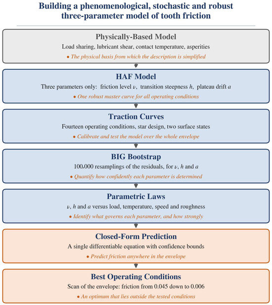
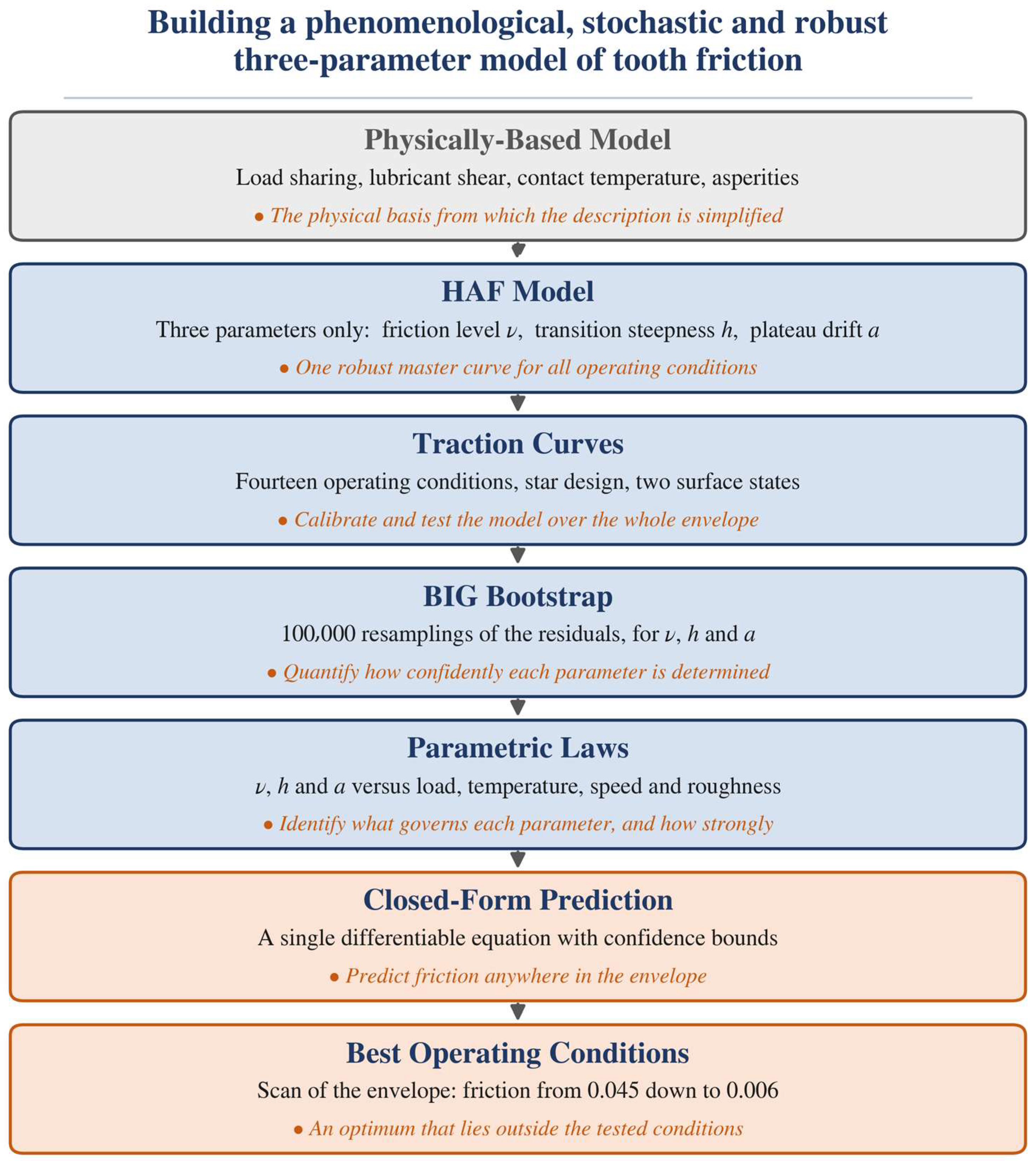
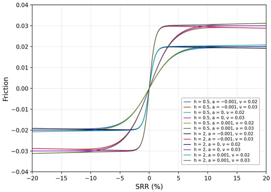
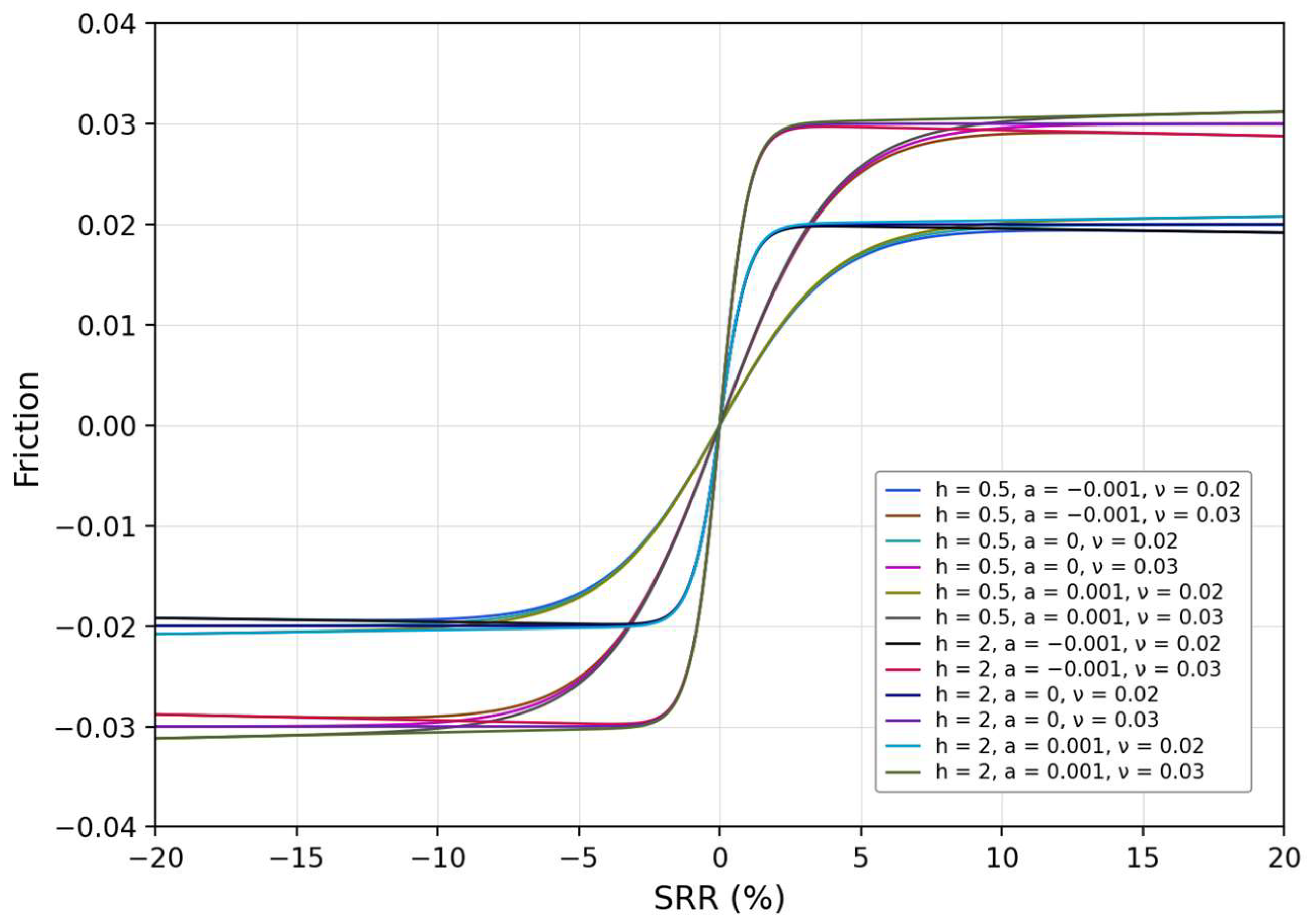
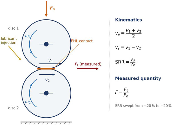
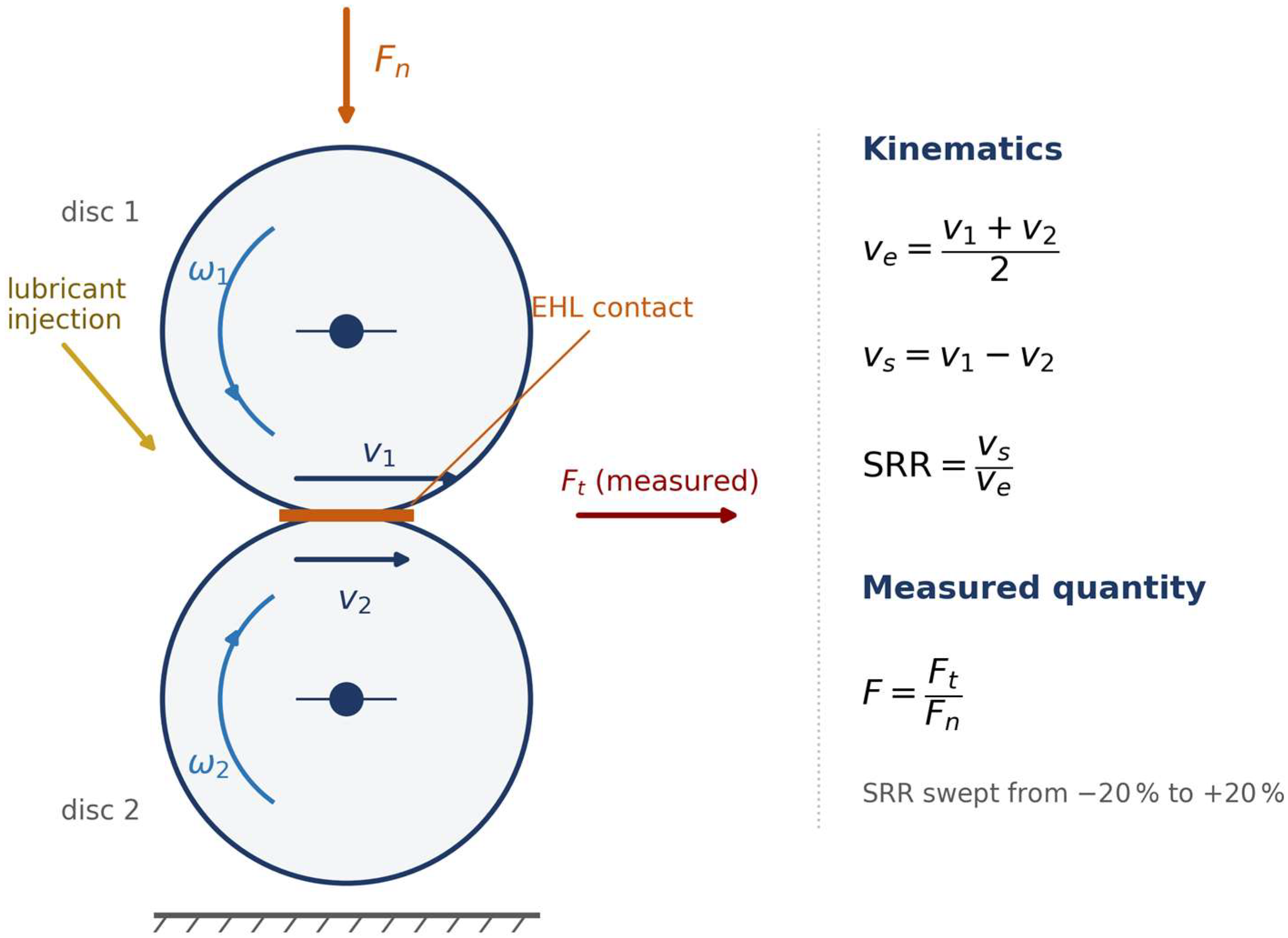
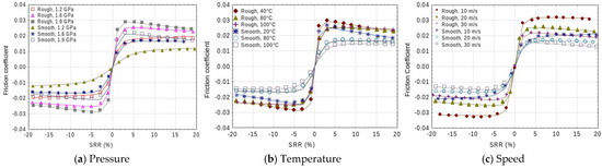
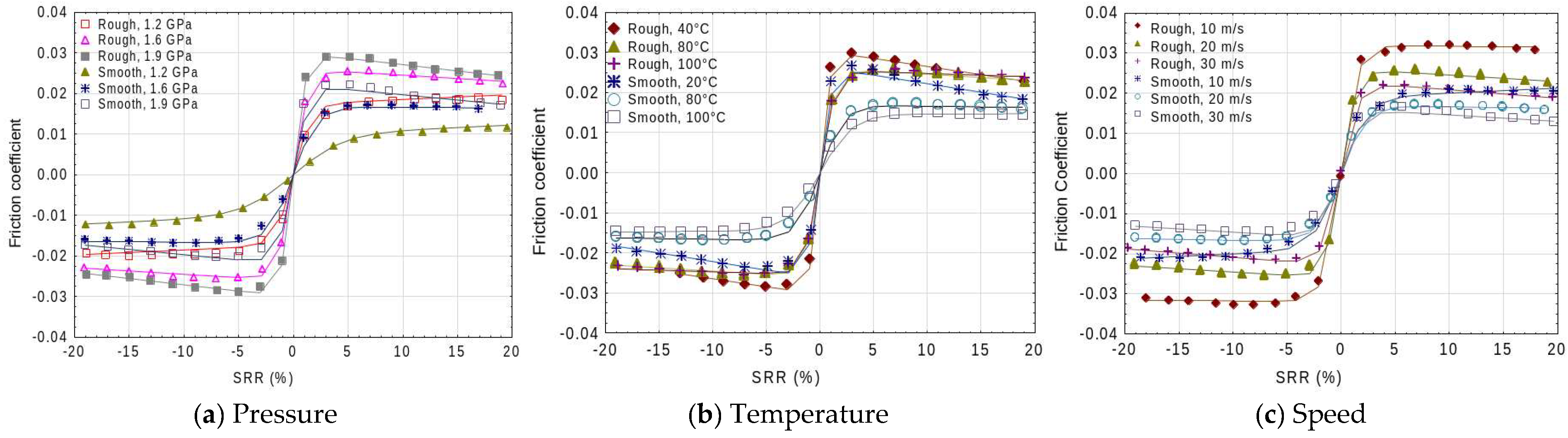
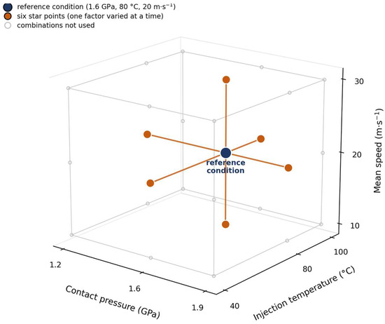
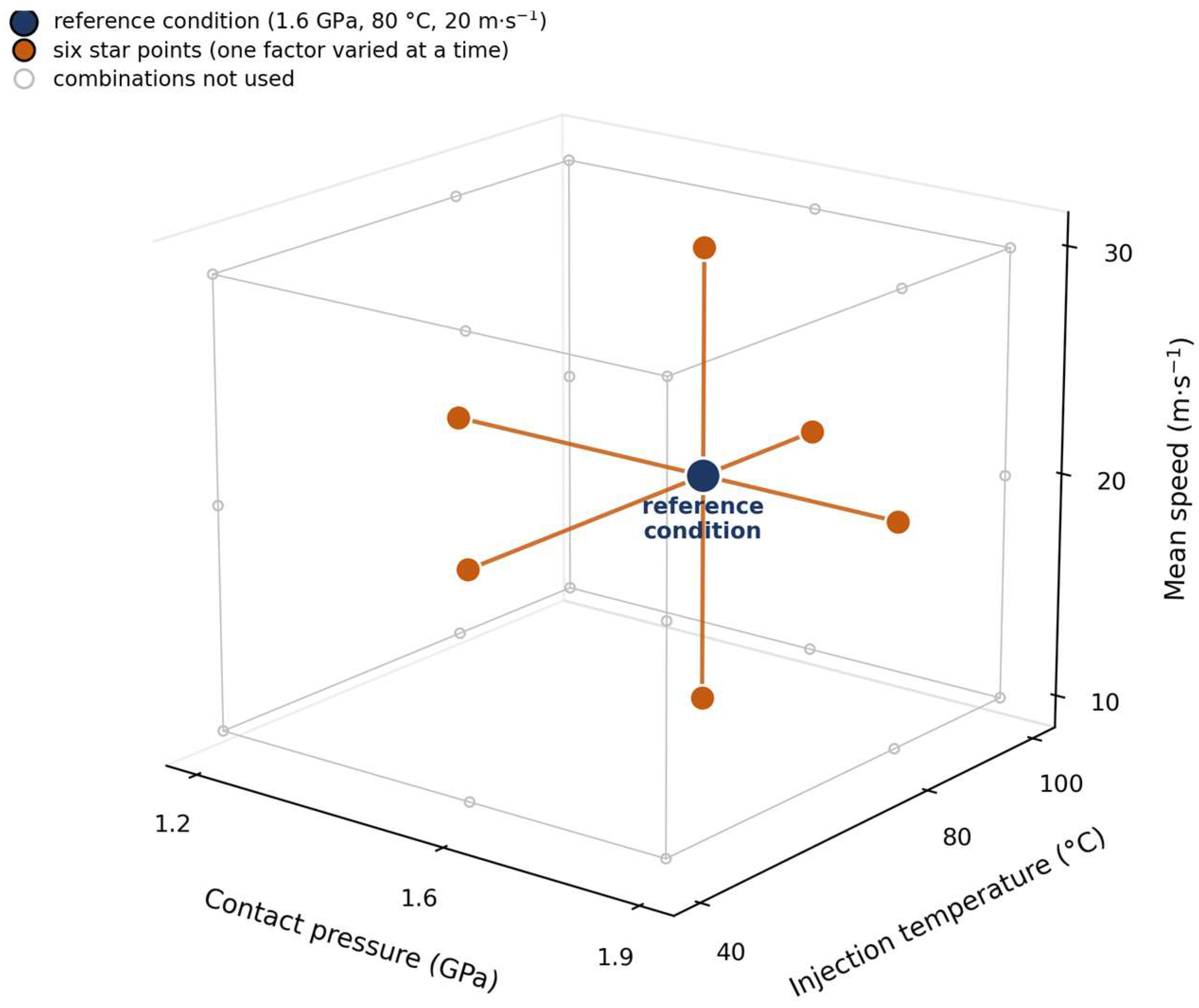
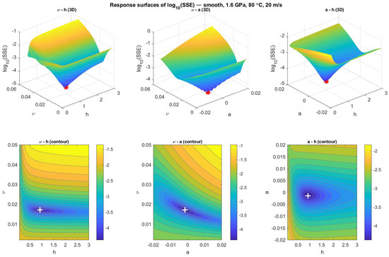
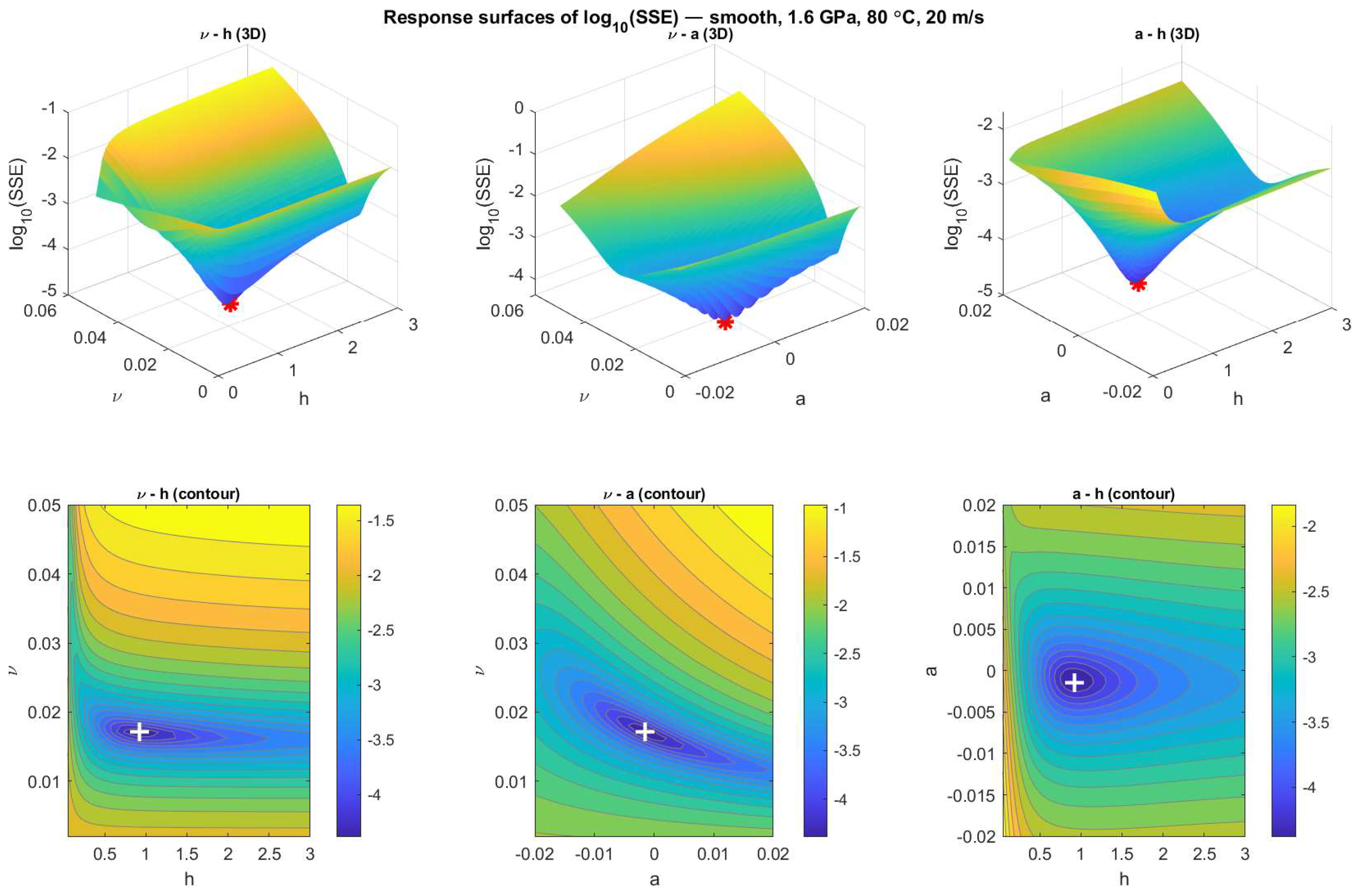
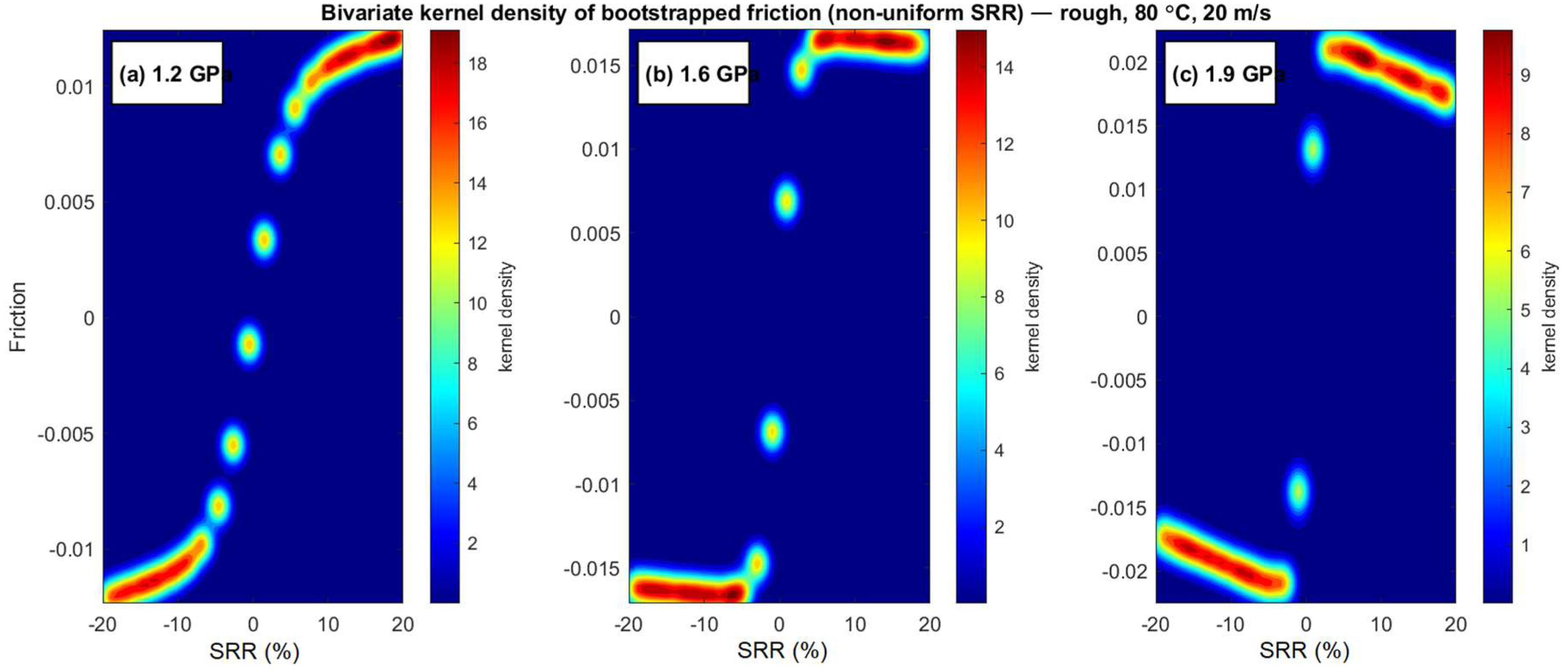
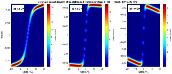
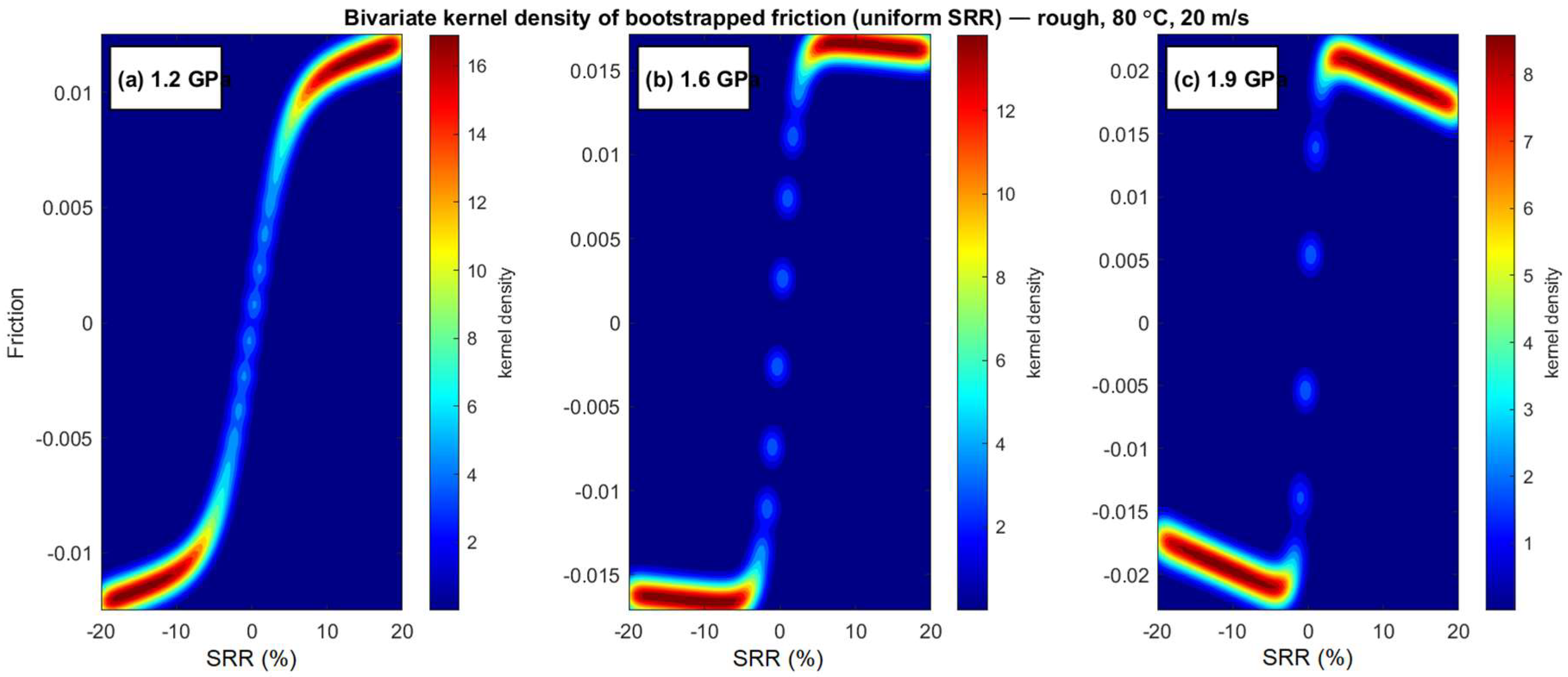
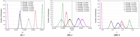
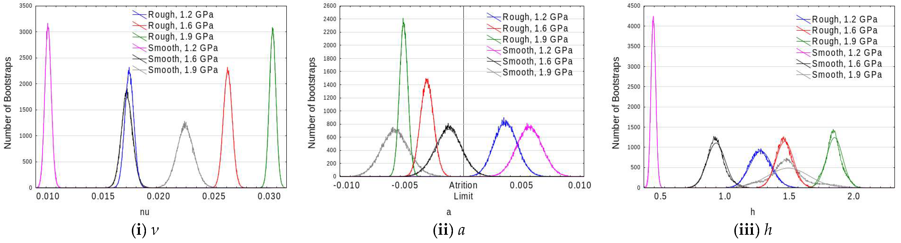
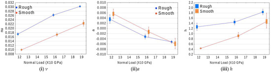
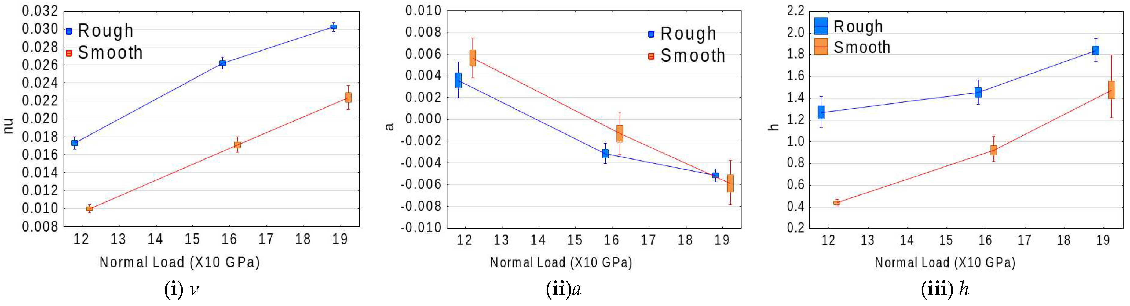
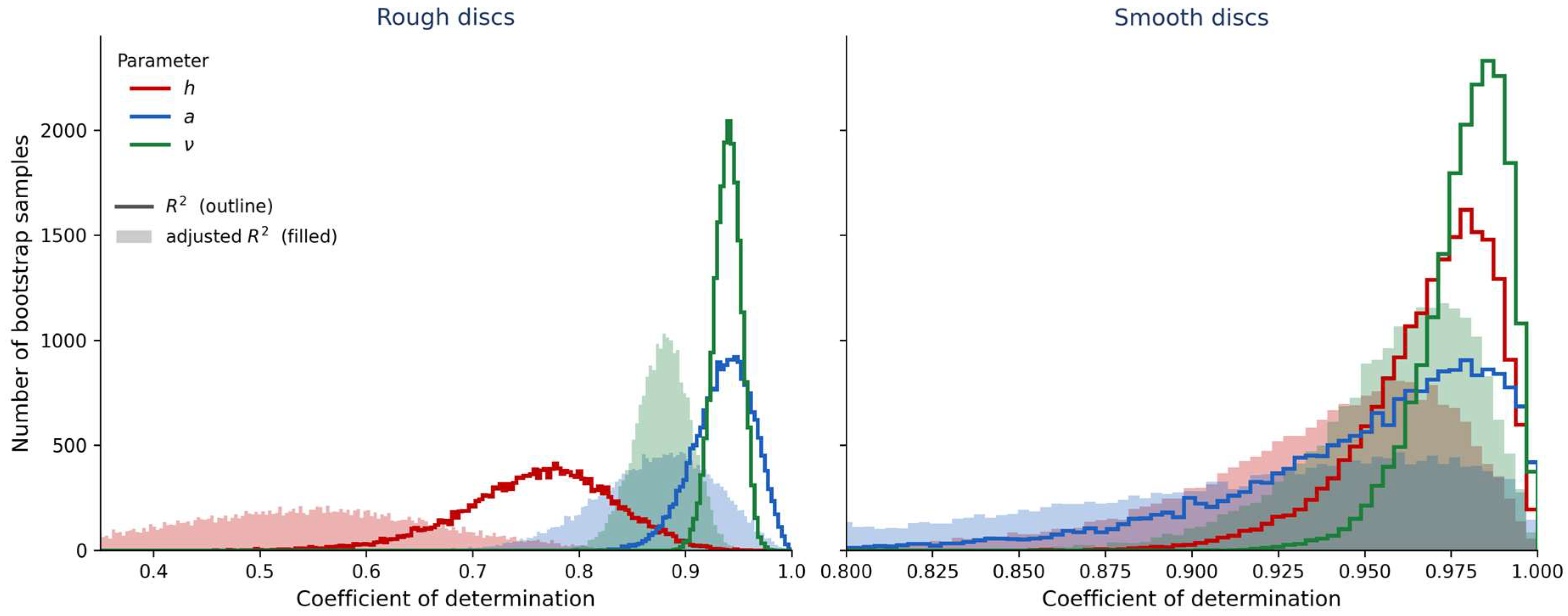
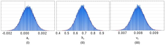
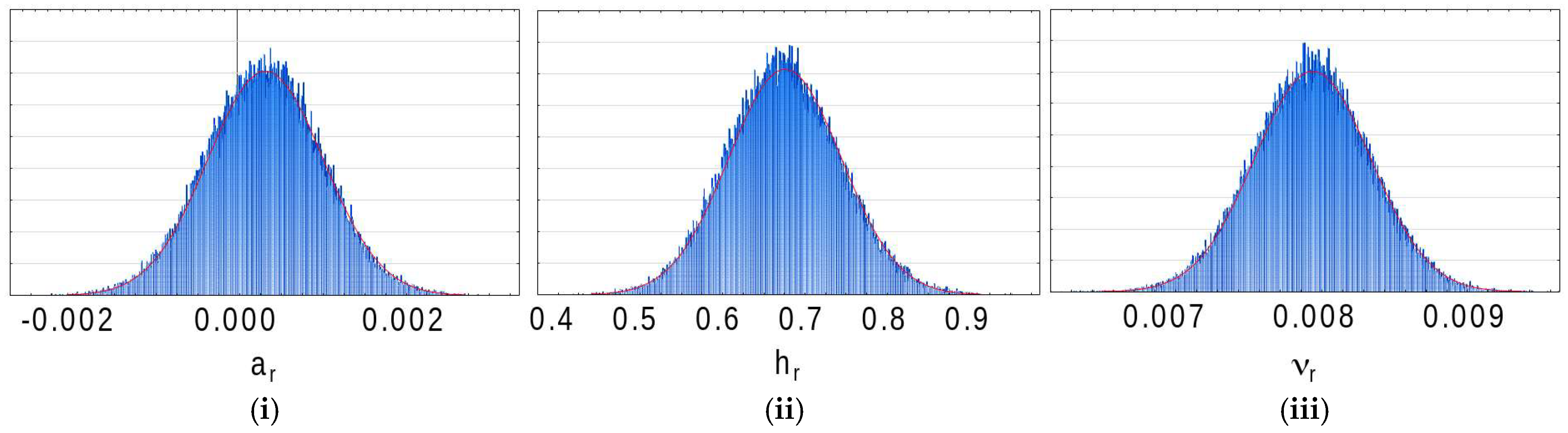
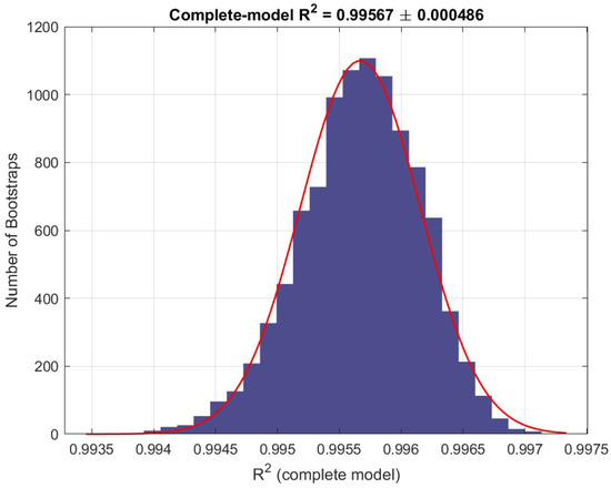
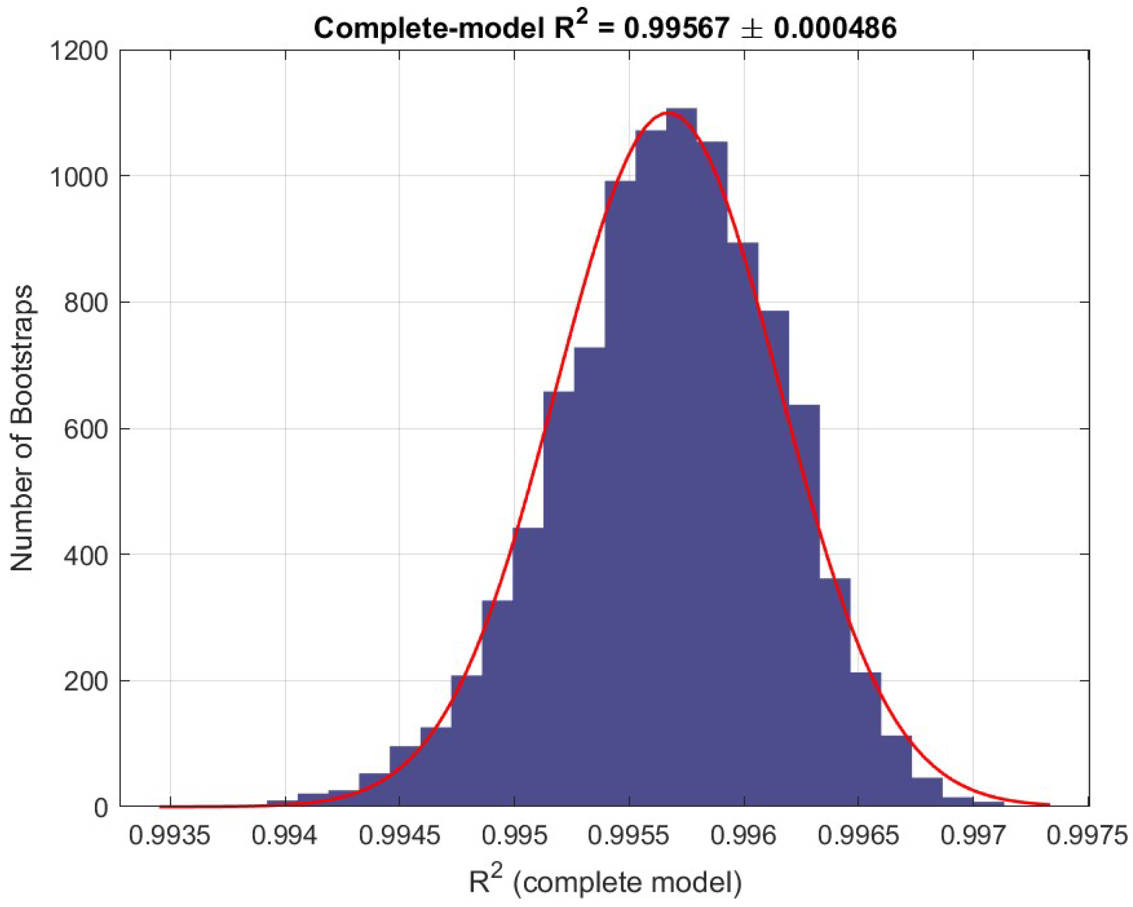
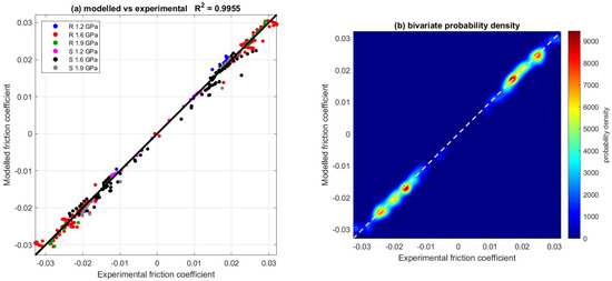
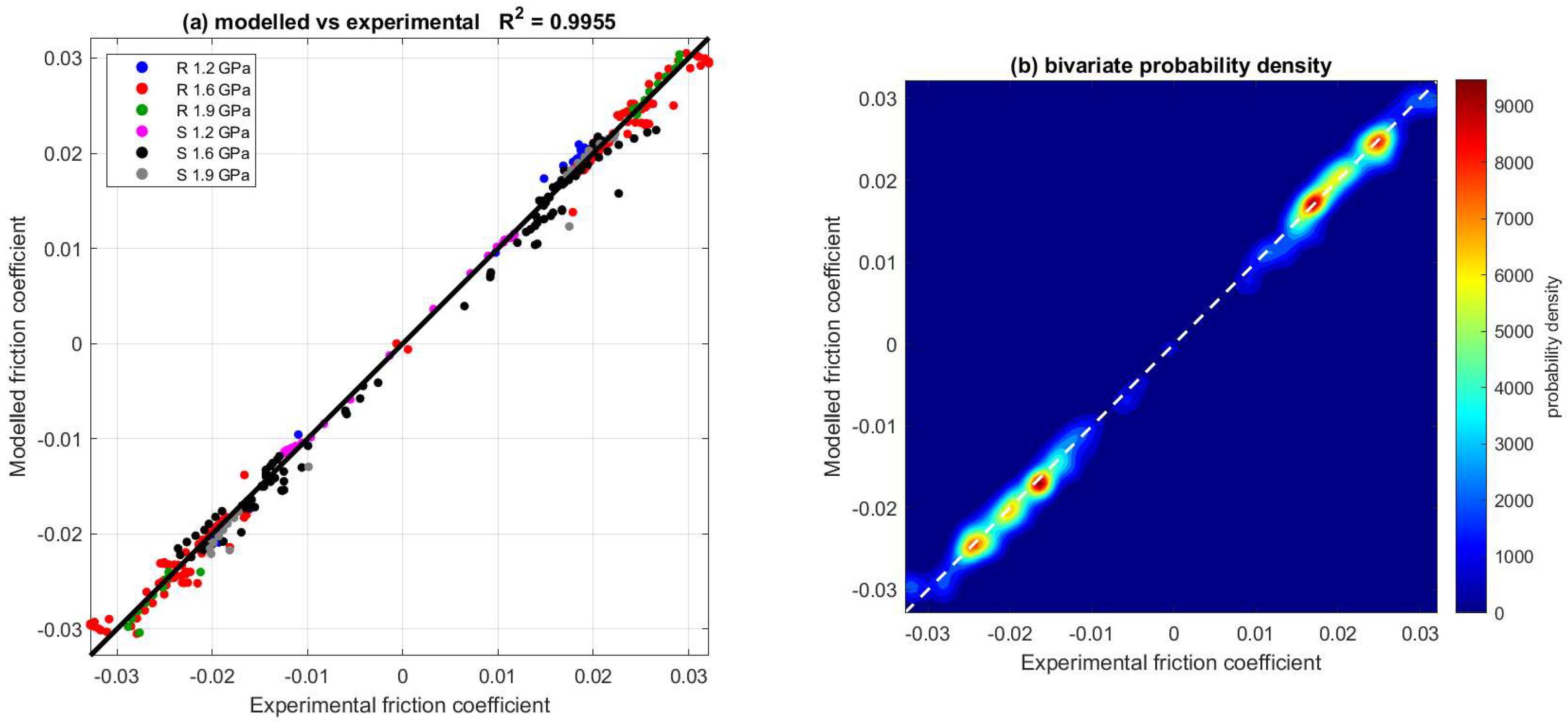
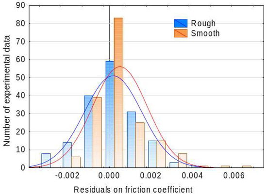
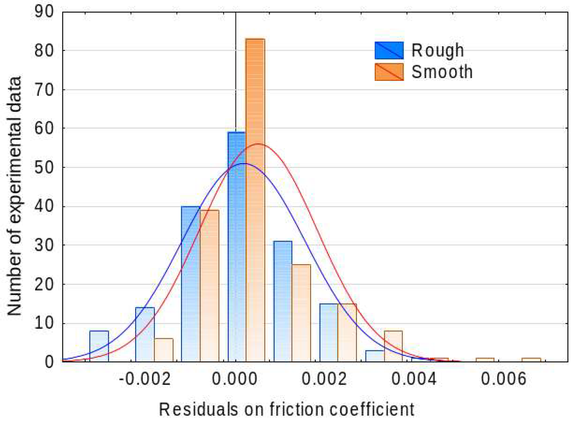
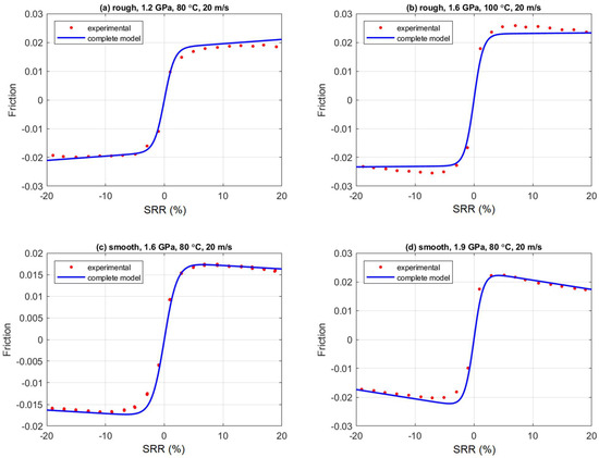
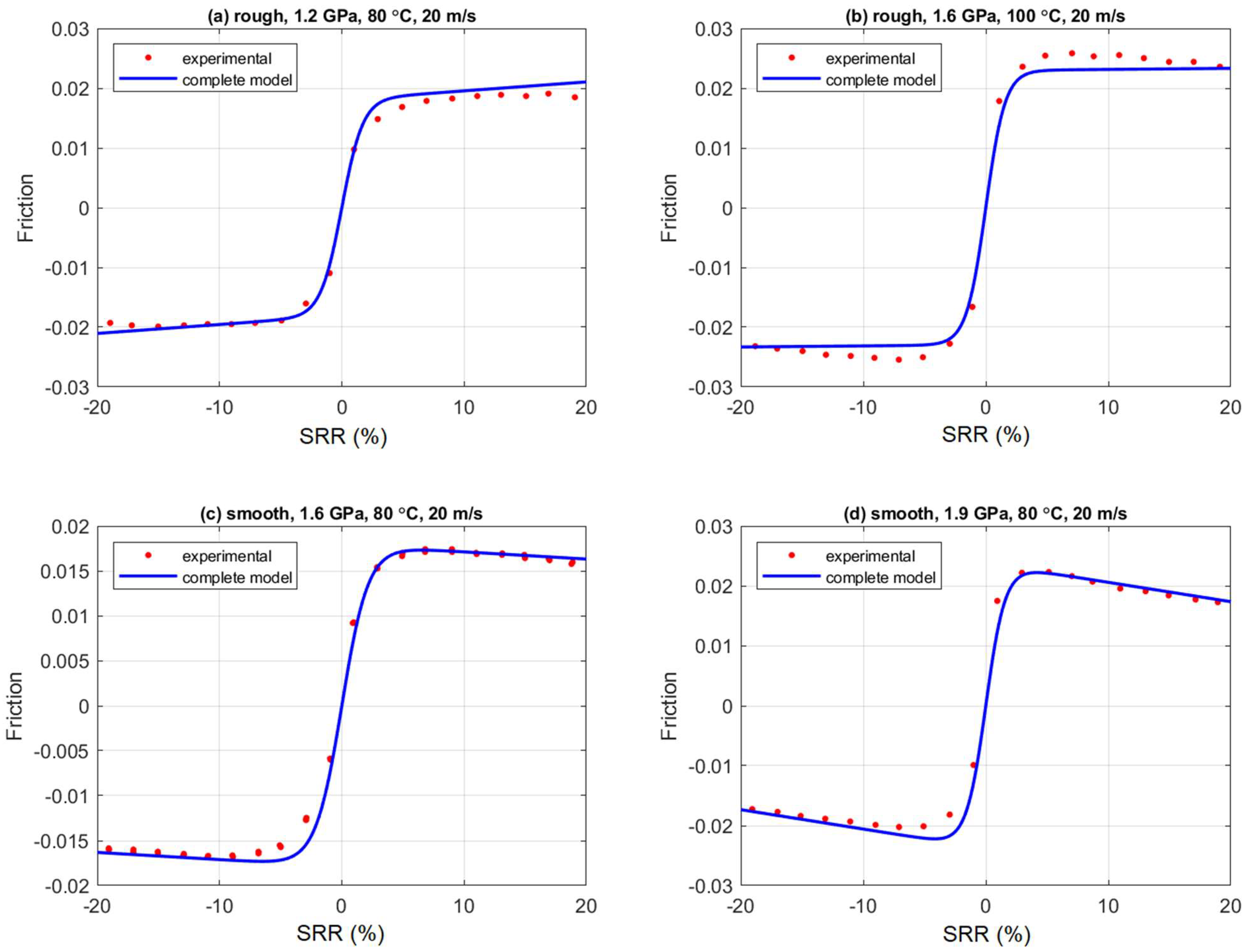
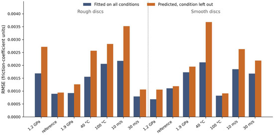
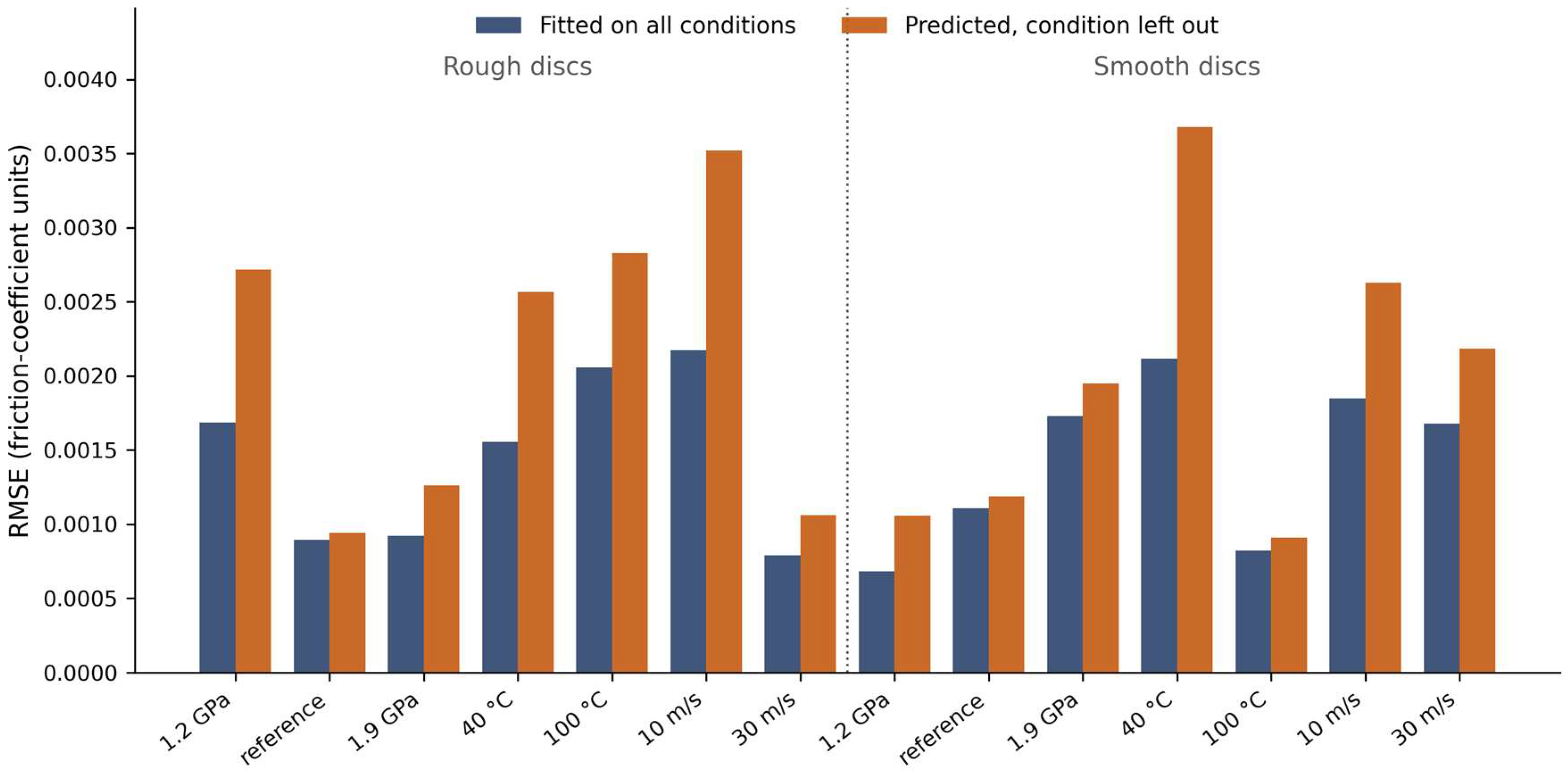
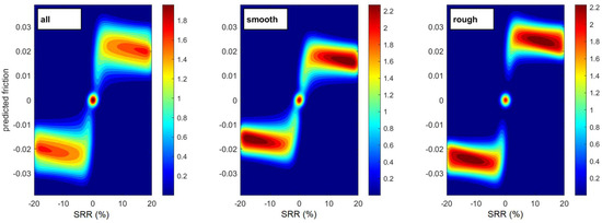
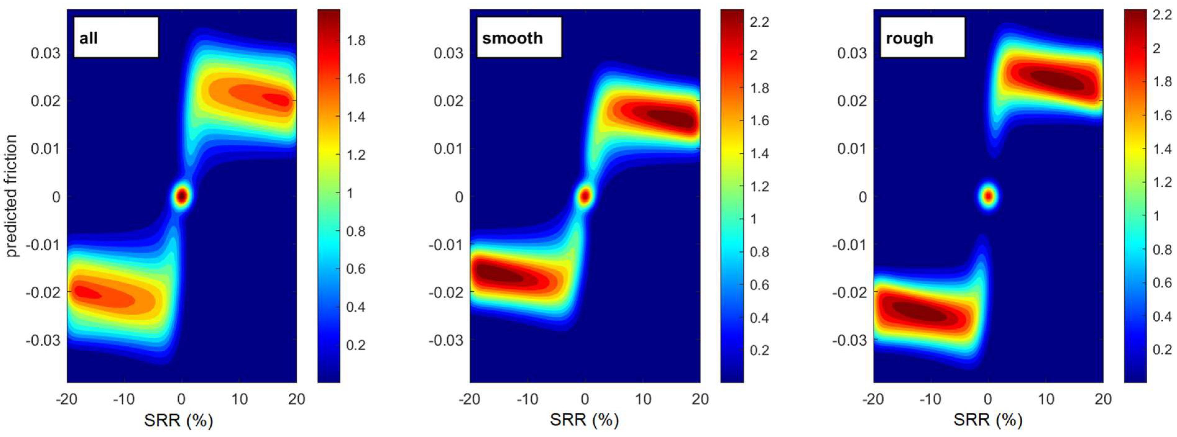
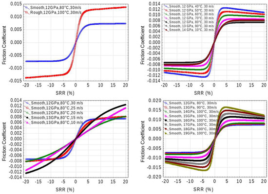
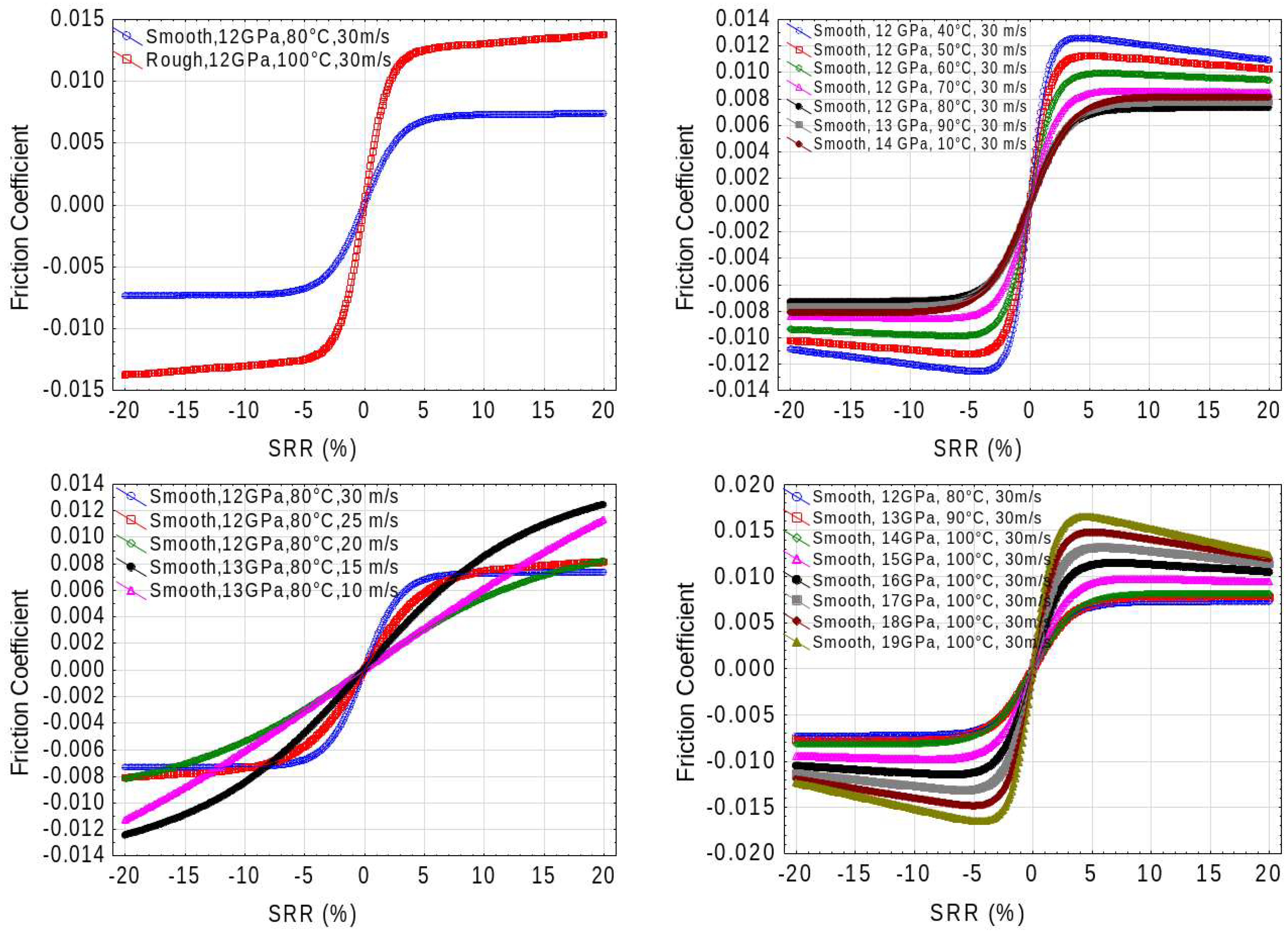
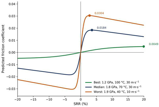
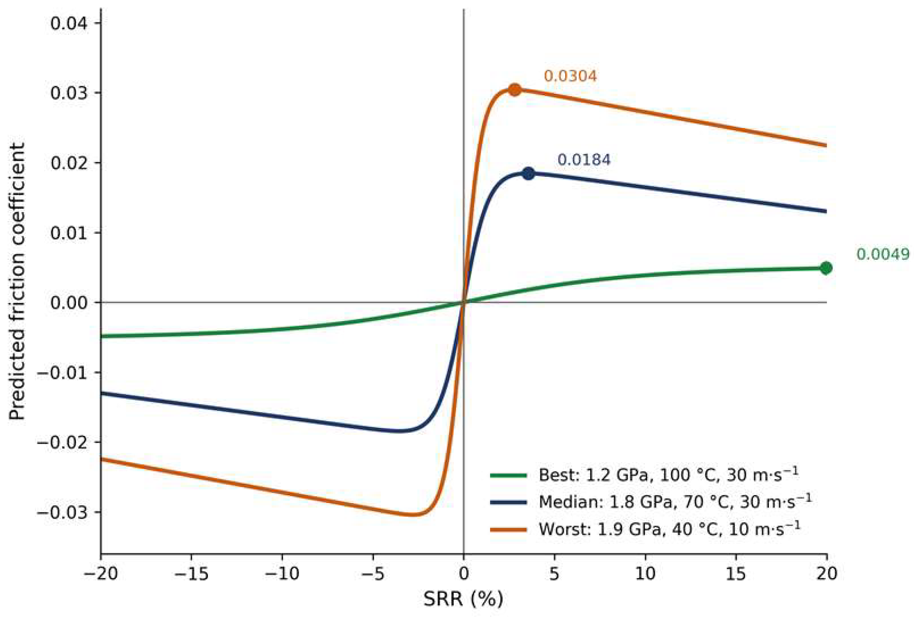

Disclaimer/Publisher’s Note: The statements, opinions and data contained in all publications are solely those of the individual author(s) and contributor(s) and not of MDPI and/or the editor(s). MDPI and/or the editor(s) disclaim responsibility for any injury to people or property resulting from any ideas, methods, instructions or products referred to in the content. |
© 2026 by the authors. Licensee MDPI, Basel, Switzerland. This article is an open access article distributed under the terms and conditions of the Creative Commons Attribution (CC BY) license.