


Abstract
Aero-engine performance prediction provides an essential basis for condition assessment and health management during ground testing. Conventional component-level models require costly calibration, whereas purely data-driven models are prone to overfitting under data-scarce conditions and generally offer limited physical interpretability. To address these limitations, this study proposes a turbofan engine performance prediction method that integrates a component-topology prior with season-aware multi-source transfer learning. Based on the main gas-path connections and the mechanical coupling between the high- and low-pressure spools, a component-topology-informed fusion prediction model (Engine-BLT) is developed. It characterizes the dynamic coupling behavior of the entire engine through component-specific feature extraction, feature propagation along the gas-flow direction, and cross-component feature fusion. In addition, multiple source domains are constructed according to seasonal information, including ambient temperature, ambient pressure, and relative humidity. A similarity-based weighting strategy is then employed to improve model adaptability under small-sample transfer-learning conditions. Finally, a component-level GasTurb model is employed to provide an independent aerothermodynamic reference under representative steady-state operating conditions. The results show that Engine-BLT achieves R2 values of 0.9650, 0.9991, and 0.9962 for corrected low-pressure-turbine outlet total temperature (T5,corr), corrected net thrust (FN,corr), and corrected high-pressure-compressor outlet total pressure (Pt3,corr), respectively, yielding the best overall prediction accuracy among the evaluated models. The season-aware weighted multi-source transfer learning (SWMT) strategy also provides the best overall performance among the investigated transfer-learning schemes. Under ground idle, maximum continuous thrust, and maximum takeoff thrust conditions, its mean absolute relative errors for Pt3,corr, T5,corr, and FN,corr are 1.17%, 0.99%, and 0.33%, respectively, which are comparable in magnitude to the steady-state aerothermodynamic reference obtained from the GasTurb model. The proposed method improves prediction accuracy under small-sample acceptance-test conditions while maintaining target-domain adaptability and physical interpretability.
1. Introduction
Aero-engines are strongly coupled and highly nonlinear thermodynamic systems, and their performance status directly affects flight safety and operational economy [1,2]. Ground testing is conducted throughout development verification, production acceptance, and maintenance support. The resulting multivariate time-series data, including temperature, pressure, rotational speed, fuel flow, and thrust, characterize the dynamic responses of the engine under both steady-state operation and operating-condition transitions, thereby providing an essential basis for performance prediction and health assessment [3,4]. However, variations in ambient conditions, test missions, and engine-to-engine characteristics often lead to pronounced data-distribution shifts across operating conditions and test batches. In addition, only limited samples are available for certain target conditions, which degrades model generalization and prediction accuracy. Therefore, accurate performance prediction under small-sample target conditions remains challenging. Effective knowledge transfer from related operating conditions is essential for improving cross-condition generalization in aero-engine applications [5,6].
Existing aero-engine performance prediction methods can be broadly classified into physics-based and data-driven approaches [7,8]. Component-level models based on aerothermodynamic principles and mass- and energy-conservation laws provide clear physical interpretation [9]. However, owing to multiphysics coupling, uncertainties in component characteristics, and engine-to-engine variations, these models often struggle to fully characterize the nonlinear responses of aero-engines under complex operating conditions and transient processes, resulting in limitations in prediction accuracy and adaptability across operating conditions [10,11].
Data-driven models, supported by the strong nonlinear approximation capability of deep learning, can directly learn the nonlinear mappings between input variables and engine performance parameters from historical test data. Owing to their high modeling efficiency, these models have been widely applied to aero-engine performance prediction. Related methods have gradually evolved from conventional statistical approaches, such as multiple linear regression [12] and partial least-squares regression [13], to machine-learning methods, including support vector regression [14] and artificial neural networks. Commonly adopted algorithms include multilayer perceptrons (MLPs) [15,16], convolutional neural networks (CNNs) [17,18,19], and deep time-series models such as long short-term memory (LSTM) networks [20,21,22], bidirectional LSTM (BiLSTM) networks [23], recurrent neural networks (RNNs) [24] and Transformers. These methods have achieved high prediction accuracy for key engine performance parameters. Nevertheless, purely data-driven models are essentially black-box models and lack explicit physical constraints, which may result in predictions with insufficient physical consistency. This limitation is particularly important because model interpretability is a major concern in engineering applications [25,26].
To combine the nonlinear representation capability of data-driven models with the physical interpretability of mechanism-based models, the integration of physical knowledge and data-driven methods has become an important research direction in intelligent aero-engine modeling. Existing approaches to incorporating physical knowledge can be broadly classified into three categories. The first constructs graph structures or dedicated network architectures according to engine component configurations and gas-path connections, thereby embedding physical-topology priors at the model-architecture level [27]. The second employs physics-informed neural networks (PINNs), in which residuals of governing equations, conservation relations, or boundary conditions are introduced into the loss function as additional constraints [28,29,30]. The third uses component-level simulation data to assist the training, calibration, or validation of data-driven models [31]. Previous studies have embedded component topology, conservation relations, and thermodynamic knowledge into neural networks, thereby improving the physical relevance and engineering credibility of model predictions. Various deep-learning architectures, including CNNs, LSTMs, GNNs, and Transformers, have been applied to aero-engine performance prediction, health monitoring, and degradation assessment [32,33,34]. Xiao et al. [35] developed a data-driven method for long-term engine degradation monitoring. Engine physical topology was embedded into an LSTM-based model to track thrust degradation over the engine lifecycle. Tang et al. [36] proposed an intelligent incremental model for exhaust gas temperature prediction. The model combines a physical-architecture-driven feature extractor with knowledge-transfer mechanisms to adapt to distribution changes among successive flight missions. Xiao et al. [37] combined a physical-structure-driven LSTM model with error-compensation methods for exhaust gas temperature prediction. Their method improved the applicability of data-driven models to aircraft-engine health management. Xiao et al. [38] proposed Engineformer, a Transformer-based digital-twin model. The compression and expansion processes are represented by encoder and decoder modules, respectively, while cross-attention is used to characterize their interactions. The model was evaluated for both exhaust gas temperature and remaining useful life prediction. These studies demonstrate the potential of integrating aero-engine physical knowledge with deep learning for performance monitoring and degradation prediction. However, previous studies have mainly focused on network architecture design, degradation tracking, error compensation, or incremental model updating.
In practical applications, for newly developed engine types, specific operating states, and acceptance-test tasks, the number of target-domain samples is often insufficient to support the training of complex deep-learning models from scratch. Transfer learning can alleviate this limitation by reusing knowledge acquired from simulation data, historical test data, or related operating conditions and adapting the pretrained model using a small amount of target-domain data. This reduces the dependence on large target-domain datasets and improves prediction accuracy and generalization under small-sample conditions [39,40]. To address limited data availability in new test scenarios and distribution discrepancies between source and target domains, Zhao and Wang proposed an adaptive-weight transfer-learning method. By combining operating-condition similarity analysis, cross-domain data calibration, dynamic weighting of source-domain samples, and target-domain fine-tuning, their method enabled model transfer between wind tunnels of different scales and improved prediction accuracy in small-sample target scenarios [41]. Berghout et al. proposed ProgNet, in which a two-layer LSTM network was pretrained using a large number of degradation trajectories generated by PrognosEase and subsequently transferred to the N-CMAPSS target domain for fine-tuning, thereby enabling remaining useful life prediction for aero-engines [42]. Existing studies have demonstrated the applicability of transfer learning to remaining useful life prediction, degradation modeling, and transient-performance modeling. However, most representative methods rely on knowledge transfer from a single-source domain to a target domain and give limited consideration of the correlations, distribution discrepancies, and relative knowledge contributions among multiple historical domains. Meanwhile, seasonal variations in temperature, pressure, and humidity alter engine inlet conditions and may induce distribution shifts in test data, whereas studies on multi-source domain construction and adaptive knowledge fusion across seasonal environments remain relatively limited [43]. When the source and target domains are weakly correlated or exhibit substantial distribution shifts, negative transfer may occur, indicating that cross-condition and cross-environment adaptability still require further improvement [44,45].
Overall, existing studies have not sufficiently investigated the architectural mapping between internal feature-propagation pathways in neural networks and the physical topology and operating logic of aero-engine components. Further limitations remain in physical interpretability, cross-condition adaptability, and transfer capability under small-sample conditions. To address these issues, this study considers a dual-spool, low-bypass-ratio, separate-flow turbofan engine and focuses on performance prediction with limited acceptance-test data. Physical-topology-guided data-driven modeling, season-aware multi-source-domain transfer learning strategy, and independent component-level mechanistic validation are investigated. The main contributions are summarized as follows:
- (1)
- A component-topology-informed fusion prediction model is proposed. Component-specific subnetworks are constructed according to the engine component configuration, gas-path information flow, and operating logic, and appropriate network structures are assigned to different components based on their data characteristics and dynamic representation requirements. In this way, physical-topology priors are embedded into the model architecture to strengthen the physical relevance of feature propagation and improve the physical consistency of the predictions.
- (2)
- A season-aware weighted multi-source transfer strategy is developed. Historical test data are divided into multiple seasonal source domains according to ambient conditions. Cosine similarity is then employed to quantify the correlation between each source domain and the target domain, based on which source-domain knowledge is adaptively weighted. This strategy reduces the risk of negative transfer caused by irrelevant source-domain information and improves cross-environment adaptability under small-sample conditions.
- (3)
- A component-level aerothermodynamic model of the target engine is established using GasTurb and calibrated under the design-point and representative steady-state off-design conditions. By comparing the response directions and variation patterns of key performance parameters obtained from the component-level and data-driven models, the trend consistency and engineering plausibility of the predictions are evaluated. This provides an independent mechanistic reference for the proposed method.
2. Data and Experimental Design
2.1. Historical Ground-Test Data and Variable Definition
The historical ground-test data used in this study were obtained from a dual-spool, low-bypass-ratio, separate-flow turbofan engine. The data were acquired during actual factory and acceptance tests and were synchronously recorded by the engine ground-test measurement and control system at an original sampling frequency of 50 Hz. The system continuously recorded multiple categories of parameters, including ambient conditions, engine control inputs, spool operating states, gas-path performance parameters, and thrust, thereby forming multivariate time-series data that characterize the complete engine ground-test process.
A total of 12 factory-test runs and five acceptance-test runs were used, denoted as F01–F12 and A01–A05, respectively. Each factory-test run contains approximately 1.9 × 10⁵–2.5 × 10⁵ original samples, whereas each acceptance-test run contains approximately 1.2 × 10⁵–1.8 × 10⁵ original samples, as summarized in Table 1. Each run constitutes a continuous and complete ground-test sequence. The relatively data-rich factory-test dataset is primarily used for baseline-model training and source-domain construction in transfer learning, whereas the more limited acceptance-test dataset is mainly used for target-domain fine-tuning and independent testing. The detailed partitioning of individual test runs for the different experiments is described in Section 2.3.
Table 1.
Overview of the historical ground-test datasets.
Each complete test run covers the principal steady-state and transient stages of a ground-test cycle, including engine start, idle, intermediate power, maximum continuous power, takeoff power, and the subsequent return to idle. The test runs differ in ambient conditions, the durations of individual operating stages, and the corresponding dynamic control processes, resulting in continuous time series with different operating characteristics. The available historical records include variable definitions, sampling information, operating-stage information, and test-run identifiers. Environmental parameters, engine control parameters, spool operating parameters, and relevant gas-path performance parameters were selected for model development, and their definitions are summarized in Table 2.
Table 2.
Measured and recorded variables used in the ground-test dataset.
Table 2 summarizes the variables retained from the historical ground-test records, including test-environment parameters (T0, P0 and RH0), gas-path performance parameters (, Pt3,corr, N1, N2, N1,corr, N2,corr, and T5,corr), the engine control parameter (PLA), and the thrust performance parameter (FN,corr).
In addition, prior to model training, a uniform data-processing procedure was applied to screen and preprocess the raw ground-test data from all test runs. Small nonzero fuel-flow readings were observed under the no-fuel condition before engine start and were primarily attributed to sensor zero offset and measurement noise; these readings were therefore set to zero during preprocessing. The instant at which the starter began driving the high-pressure spool was defined as the beginning of the valid test sequence, and the preceding long-duration stationary records were removed. The same preprocessing criteria were consistently applied to all test runs, yielding continuous operating-condition time series that satisfy the basic physical constraints of engine operation. The corrected net thrust FN,corr, corrected high-pressure-compressor outlet total pressure Pt3,corr, and corrected low-pressure-turbine outlet total temperature T5,corr were selected as the three prediction outputs, while the remaining selected variables were used as model inputs according to the variable-to-component mappings defined in the subsequent modeling framework.
The corresponding corrected ground-test records were used consistently as the reference data for model evaluation. Accordingly, the prediction errors reported in this study represent the differences between the model outputs and these reference data, enabling a consistent comparison of predictive performance across models using the same reference data.
2.2. Data Processing
To prevent differences in physical units and numerical scales from disproportionately affecting model training, z-score standardization was applied to both the input and output variables. The standardization statistics were calculated exclusively from the training set, and the validation and test sets were transformed using the training-set statistics to prevent data leakage.
For an arbitrary variable , its z-score-standardized form is given by:
In Equation (2), zi,j denotes the original value of the jth variable in the ith sample, is the corresponding standardized value, μj,train and σj,train are the mean and standard deviation of the jth variable calculated from the training set, respectively, and ε is a small positive constant introduced to prevent division by zero. The training-set mean and standard deviation are defined as follows, where Ntrain denotes the number of training samples. Both μj,train and σj,train are calculated exclusively from the training set; the corresponding statistics are not recalculated separately for the validation or test set.
A sliding-window sampling strategy was adopted along the temporal dimension so that each model input contained observations from multiple historical time steps, thereby incorporating the dynamic evolution of the engine. As illustrated in Figure 1, the sliding window is governed by the following two adjustable parameters: the window length L and the stride d. The window length L determines the number of historical time steps included in each input instance, whereas d specifies the number of time steps by which the window advances when generating the next sample. For example, when L = 3 and d = 2, prediction of the target value at time t uses the sensor measurements at t, t − 1, and t − 2, and the window is subsequently advanced by two time steps to generate the next sample. The values of L and d were selected by jointly considering the engine dynamic-response characteristics, sample redundancy, and validation-set error.
Figure 1.
Schematic of the sliding-window sampling strategy.
2.3. Dataset Partitioning Strategy
For the baseline comparison, eight factory-test runs (F01–F08) were used. F01–F06 were assigned to model training, F07 to validation and hyperparameter selection, and F08 to independent testing. The same run-wise partition was used for all baseline models, and each model was independently trained five times to reduce the influence of training randomness. The data were partitioned by complete test runs rather than by randomly splitting individual time-series samples. This prevents highly correlated adjacent samples from the same 50 Hz test sequence from appearing in both the training and test sets and thereby avoids information leakage.
For the transfer-learning comparison, the factory-test dataset contains 12 complete runs (F01–F12), whereas only five acceptance-test runs (A01–A05) are available. Therefore, the relatively data-rich factory-test dataset was used as the primary source domain, while the acceptance-test dataset was treated as the data-limited target domain. To evaluate target-domain generalization without using test information during model adaptation, the five acceptance-test runs were partitioned in a run-wise rotation. In each round, one acceptance-test run was reserved as the independent target test set, one was used as the target-domain fine-tuning set, and the remaining three formed the secondary source domain. Each of A01–A05 served once as the independent test run, resulting in five evaluation rounds. The role assignment of each run was fixed before model training and kept identical for all transfer-learning schemes to ensure a fair comparison. The independent test run was excluded from pretraining, fine-tuning, calculation of standardization statistics, source-domain weight estimation, hyperparameter selection, and model selection. The final performance was reported as the mean evaluation metrics over the five rounds. The detailed partitioning scheme is summarized in Table 3.
Table 3.
Run-wise dataset partitioning for baseline-model and transfer-learning evaluations.
3. Methodology
The turbofan-engine performance prediction method proposed in this section comprises the following three modules: the component-topology-informed performance prediction network (Engine-BLT model), the season-aware weighted multi-source transfer learning (SWMT) strategy, and a GasTurb-based component-level performance model. First, BiLSTM, Transformer, and Transformer-BiLSTM are adopted as data-driven baseline models. Guided by the connectivity of the main gas path and the mechanical coupling relationships of the high- and low-pressure spools, Engine-BLT is developed by integrating heterogeneous component-level feature extraction with engine-level feature fusion. Second, to address the data-distribution discrepancy between factory and acceptance tests, the following four schemes are comparatively evaluated: no transfer, single-source transfer, randomly partitioned multi-source weighted transfer, and season-aware four-source weighted transfer. Finally, an independent component-level performance model is established using GasTurb 13 to provide an aerothermodynamic reference for evaluating parameter variation trends under representative steady-state conditions. The overall framework of this study is illustrated in Figure 2, which also presents representative time-series profiles of selected variables from factory and acceptance ground tests in its “Data Source” section.
Figure 2.
Overall framework of the study.
3.1. Turbofan Engine Topology and Modeling Rationale
A dual-spool, low-bypass-ratio, separate-flow turbofan engine is considered in this study. As shown in Figure 3, its main gas path consists sequentially of the inlet, fan, low-pressure compressor, high-pressure compressor, combustor, high-pressure turbine, low-pressure turbine, and core and bypass exhaust nozzles. The physical architecture and operating principles of the turbofan engine can be summarized by three fundamental physical relationships. First, each core component performs a specific function in the thermodynamic cycle: the compressors compress the incoming air, the combustor enables fuel-air mixing and heat release through combustion, and the turbines extract mechanical power from the expansion of high-temperature gas. Second, the components do not operate independently but work cooperatively under strict matching constraints. The compressor and turbine on the same spool rotate at the same shaft speed. Under steady-state operation, the turbine output power balances the compressor power demand and mechanical losses. During transient operation, the resulting power imbalance governs spool acceleration or deceleration. Mass-flow continuity is also maintained across adjacent component interfaces. Third, the working fluid undergoes compression, combustion, expansion, and exhaust sequentially along the gas path, forming a continuous and unidirectional thermodynamic cycle. These physical relationships, together with the engine structural information, are incorporated as prior physical knowledge into the subsequent component-topology-informed modeling framework.
Figure 3.
Schematic of the turbofan engine.
3.2. Performance Prediction Model
3.2.1. Baseline Prediction Models
Aero-engine ground-test measurements are multivariate time series with pronounced temporal dependencies. Therefore, BiLSTM, Transformer, and Transformer-BiLSTM are adopted as representative sequence-modeling baselines. These models represent recurrent, attention-based, and hybrid architectures, respectively. All three models use the same preprocessing procedure, prediction targets, and data partitioning and differ mainly in their feature extraction and temporal modeling mechanisms.
LSTM uses forget, input, and output gates to control information retention, updating, and output, thereby alleviating the vanishing-gradient problem of conventional recurrent neural networks [46]. BiLSTM consists of forward and backward LSTMs and captures contextual information in both directions [47], as shown in Figure 4. Its output is expressed as follows:
where and are the forward and backward hidden states, respectively.
Figure 4.
Schematic of the BiLSTM architecture.
The Transformer architecture introduced by Vaswani et al. [48] uses self-attention to model dependencies among different sequence positions without recurrent computation. In this study, positional encoding is first added to the input sequence to preserve temporal order. The query, key, and value matrices are then obtained through linear projections, while multiple attention heads extract features in parallel representation subspaces. Given the input feature matrix H, the query, key, and value matrices and the scaled dot-product attention are defined as:
Q = HWQ, K = HWK, V = HWV
In Equations (6) and (7), dk denotes the dimension of the key vectors. Multi-head attention captures sequence dependencies in parallel feature subspaces. Its output passes through residual connections, layer normalization, and a feed-forward network to form a global feature representation.
The Transformer-BiLSTM model first captures global dependencies using the Transformer. Two BiLSTM layers then extract local dynamics and bidirectional temporal features, followed by a fully connected output layer. This architecture combines the long-range modeling capability of the Transformer with the dynamic representation capability of BiLSTM.
All three are generic data-driven architectures used only as baselines to compare conventional networks with the proposed component-topology model.
3.2.2. Engine-BLT Model
Building on the Transformer-BiLSTM baseline, the component functions, matching constraints, and unidirectional gas-path propagation described in Section 3.1 are encoded as architectural priors to develop the Engine-BLT model.
Specifically, a separate subnetwork is assigned to each engine component and connected along the gas-flow direction. The subnetwork type is selected according to the temporal characteristics of its inputs and the component function. BiLSTM is used for components associated with rotational-speed and fuel-flow responses to capture temporal dependencies during acceleration and deceleration. The fan subnetwork employs a CNN along the time dimension to extract local fluctuations while preserving sequential outputs. Because the exhaust nozzle contains no rotating machinery and is mainly governed by the upstream turbine-exit state and ambient back pressure, it is modeled using a time-distributed fully connected layer. The same mapping parameters are shared across all time steps, projecting local inputs into a unified latent space without altering the temporal dimension. The component features are then fused and fed into a Transformer encoder to capture global coupling among components. Two BiLSTM layers subsequently perform further temporal modeling.
Additionally, the input variables are not concatenated indiscriminately but assigned to component subnetworks according to their physical meanings and component associations. Ambient temperature, pressure, and humidity define the inlet boundary conditions; fuel flow and power lever angle describe combustor energy input and engine control state; and the high- and low-pressure spool speeds and their rates of change represent steady-state operating levels and transient rotor dynamics, respectively. The speed derivatives are introduced to further characterize rotor dynamics during transient operation.
In Equation (8), Nj,t denotes the rotational speed of spool j at time t; is its rate of change; Δt is the sampling interval between adjacent time steps used to calculate the spool-speed derivative; and j denotes the spool index.
Each component subnetwork extracts local temporal features and fuses them with the hidden state from the upstream component, enabling progressive state modeling along the main gas path. After preprocessing, the global input vector at time t is defined, and component-level local inputs are constructed according to the gas-path topology and spool coupling. The local input window of component c is given by:
Xc,t = Sc(Xt), c = 1,2,…,C,
In Equations (9) and (10), Sc denotes the variable-selection operator for the component c. Each subnetwork selects the variables relevant to its physical function from the global input window, with c = 1, ⋯, 8 representing the eight component subnetworks.
Along the main gas path, latent features are propagated sequentially through the component subnetworks. The inlet subnetwork receives only its local input window:
Z1,t = X1,t
h1,t = F1(Z1,t)
For each subsequent component, the subnetwork input comprises its local input window and the output features of the preceding component:
Zc,t = [Xc,t, hc−1,t], c = 2, 3, …, C
hc,t = Fc(Zc,t)
In Equations (13) and (14), Zc,t denotes the actual input to component subnetwork c, hc−1,t and hc,t are the latent features output by the preceding and current component subnetworks, respectively, and Fc( ) denotes component subnetwork c. The local inputs, network types, and feature-propagation relationships are listed in Table 4.
Table 4.
Architecture and feature propagation of the component subnetworks.
The latent features from the component subnetworks are arranged into a component feature sequence following the main gas-path order:
The component feature sequence Ht is then fed into the Transformer encoder, where multi-head self-attention adaptively learns the global coupling among the compressor, combustor, turbine, and nozzle under different operating conditions. The fused features at each time step form a sequence that is passed through two BiLSTM layers. The first retains the full sequence to capture dependencies among condition transitions, acceleration/deceleration, and steady-state stages, while the second compresses the sequence into an engine-level state representation. A fully connected layer then predicts the performance parameters. The model output is expressed as corrected low-pressure-turbine outlet total temperature (T5,corr), corrected net thrust (FN,corr), and corrected high-pressure-compressor outlet total pressure (Pt3,corr), representing the predicted turbine-exit total temperature, corrected thrust, and high-pressure-compressor outlet total pressure, respectively. Figure 5 shows the Engine-BLT architecture.
yt = fq(Xt), q ∈ {T5,corr, FN,corr, Pt3,corr}
Figure 5.
Architecture of the proposed Engine-BLT model.
3.2.3. Model Training
Training hyperparameters directly affect model accuracy and the reliability of the results. Therefore, key hyperparameters are optimized individually within commonly used ranges, as listed in Table 5.
Table 5.
Hyperparameter search ranges.
Taking the BiLSTM baseline as an example, hyperparameters are optimized using a one-factor-at-a-time strategy. First, the number of epochs is varied while fixing the batch size at 128 and the dropout rate at 0.5. The optimal batch size is then determined using the selected epoch value, followed by optimization of the dropout rate. Figure 6 shows the prediction results under different hyperparameter settings.
Figure 6.
Effects of different hyperparameter settings on the prediction performance of the BiLSTM baseline: (a) dropout rate; (b) batch size; (c) number of epochs.
The same procedure was applied to all models. Batch size was selected to balance training efficiency and accuracy, while the number of epochs was selected to provide sufficient model convergence. The optimal hyperparameters are listed in Table 6.
Table 6.
Optimal hyperparameters of the evaluated prediction models.
Each model was independently trained five times to reduce the effect of training randomness. Experiments were conducted on an Intel Core i7-12650H processor with 64 GB RAM and an NVIDIA GeForce RTX 3050 GPU with 8 GB memory. Python 3.9 and Keras 2.10.0 were used. Under the same hardware and software environment, the total training times of BiLSTM, Transformer, Transformer-BiLSTM, and Engine-BLT were 36.7, 31.2, 44.7, and 49.0 min, respectively. Engine-BLT required 49.0 min for 150 epochs, corresponding to 19.6 s per epoch. Although its more complex architecture resulted in a moderately higher training cost, the computational costs of all evaluated models remained within the same order of magnitude.
3.3. SWMT Strategy
Factory and acceptance tests differ in ambient conditions, test procedures, and engine operating states. These differences lead to distribution shifts and reduce the applicability of a model trained only on factory-test data. Transfer learning reuses knowledge acquired from a related source domain to improve learning in a target domain with limited data [49]. To improve prediction performance when only limited target-domain data are available, a transfer-learning framework is developed based on Engine-BLT.
The transfer process consists of four main stages. First, historical data are organized into one or multiple source domains, while a small amount of acceptance-test data is reserved as the target adaptation set. A separate acceptance-test run is used only for independent testing. Second, the source-domain data are used to train Engine-BLT and obtain transferable representations. For the multi-source schemes, the contribution of each source domain is determined according to its similarity to the target adaptation data. Third, the pretrained model parameters are transferred to the target-domain model. The front-end representation layers are frozen, whereas the back-end BiLSTM and fully connected layers are fine-tuned using the target adaptation set. Finally, the adapted model is evaluated on the independent target test run.
In SWMT, seasonal information is used to construct multiple source domains, whose contributions are then determined according to their feature-space similarity to the target adaptation set. The detailed transfer and weighting procedures are described below.
3.3.1. Transfer-Learning Formulation and Fine-Tuning Strategy
In each transfer-learning round, the source-domain training set, target-domain adaptation set, and independent target test set are denoted as follows:
In Equations (18)–(20), X denotes the multivariate time-series input constructed using a sliding window, and y is the corresponding performance label. Ns, Nad, and Nte are the numbers of samples in the source training, target adaptation, and independent target test sets, respectively. The three sets have different functions throughout transfer learning. The source set is used for pretraining, whereas the target adaptation set is used for target-specific fine-tuning and, in the multi-source schemes, source-domain weight estimation. The independent target test set is used only for final performance evaluation. To prevent information leakage, the test set is excluded from the calculation of standardization statistics, source-domain weight estimation, model training, fine-tuning, hyperparameter selection, and model selection.
For transfer learning, Engine-BLT is divided into a shared front end and a target-adaptable back end. The front end includes component subnetworks, gas-path feature propagation and fusion modules, and Transformer encoder, while the back end comprises two BiLSTM layers and fully connected layers. Source-domain pretraining, parameter transfer, and target-domain fine-tuning are expressed as follows:
θfront = {θcomp, θfus, θTr},
θback = {θBiLSTM, θFC},
θ = {θfront, θback},
In Equations (21)–(26), fθ( ) denotes the internal mapping of Engine-BLT, θs∗ denotes the full parameter set obtained from source-domain pretraining, and denotes the initial target-domain parameters. All pretrained weights are transferred to the target-domain model. During fine-tuning, the transferred front-end parameters are frozen, while only the back-end BiLSTM and fully connected parameters θback,t are updated.
This strategy preserves the component topology, cross-component correlations, and shared high-level representations learned from the source domain, while adapting temporal features and output mappings using limited target-domain data, thereby reducing the risk of overfitting from updating all network parameters [50].
3.3.2. Similarity-Weighted Multi-Source Domain Adaptation
A single-source domain may not sufficiently cover the environmental and operating-state distributions encountered in the target acceptance tests. Multi-source domain adaptation can exploit complementary knowledge from source domains with different distributions [51,52]. Therefore, the available historical data are organized into multiple source domains. In SWMT, seasonal information is used as a practical grouping criterion to organize historical data with different distributions of ambient temperature, pressure, and relative humidity. The seasonal label itself is not used as a model input; it only determines how the source data are grouped. The acceptance-test runs used in the source domains do not overlap with those used for target-domain adaptation or independent testing, thereby preventing data leakage. The m-th source domain is defined as follows:
The SWMT procedure contains the following three successive steps: initial feature-space construction, source-domain weight estimation, and similarity-weighted multi-source pretraining. After weighted pretraining, the resulting parameter set is transferred to the target-domain model and fine-tuned according to the strategy described in Section 3.3.1.
Transferability varies across source domains. Their weights are therefore determined by the similarity between the source-domain and target-adaptation feature centroids in the shared feature space. First, unweighted pretraining is performed on the pooled multi-source data to obtain an initial shared feature extractor, . Its parameters are then frozen, and the feature centroids of the m-th source domain and target adaptation set are calculated as follows:
The subsequent similarity is therefore evaluated using the learned domain representations rather than the raw ambient variables directly. Target-domain labels are excluded from feature-centroid and source-weight calculations. The cosine similarity and normalized weight between the m-th source domain and the target adaptation set are defined as follows:
In Equations (30) and (31), cm denotes the directional similarity between the feature centroids of the m-th source domain and the target adaptation set in the shared feature space, and ε is a small constant preventing division by zero. This metric measures first-order centroid similarity rather than the full distribution discrepancy in variance, covariance, or higher-order statistics. Softmax converts potentially negative cosine similarities into non-negative source-domain weights that sum to one.
The loss for each source domain is averaged independently to reduce the direct effect of unequal domain sizes. The similarity-weighted multi-source pretraining objective is defined as follows:
Source-domain weights remain fixed during weighted pretraining and scale each domain loss without participating in backpropagation through the similarity branch. Domains closer to the target feature centroid receive higher weights, reducing the influence of less relevant domains on parameter updates.
The following four schemes are compared: no transfer learning baseline, single-source transfer learning model, random multi-source transfer learning model, and the SWMT strategy. Figure 7 illustrates their prediction workflows.
Figure 7.
Workflows of the four transfer-learning schemes.
3.4. Component-Level Performance Modeling with GasTurb
To assess the predictions from an aerothermodynamic perspective, a component-level model of the target dual-spool, separate-flow turbofan engine was developed in GasTurb 13. The model includes the inlet, fan, bypass duct, low- and high-pressure compressors, combustor, high- and low-pressure turbines, and core and bypass nozzles. Engine matching is solved through mass-flow continuity, spool power balance, nozzle matching, and component-map interpolation. GasTurb results serve only as a mechanistic reference for evaluating trend consistency and engineering plausibility.
3.4.1. Cycle Reference Point and Design-Point Matching
Ground takeoff steady state was selected as the cycle reference point for the GasTurb model. This high-power condition reflects the main gas-path characteristics and provides key parameters, including net thrust, fuel flow, spool speeds, turbine-exit total temperature, and high-pressure-compressor outlet total pressure, making it suitable for design-point matching.
Table 7 lists the main design-point inputs and matching parameters of the GasTurb model. The design-point cycle was first calculated to determine key station parameters and shaft-power distribution. For rotating components, the resulting design-point parameters were used to scale their characteristic maps. Non-rotating components were defined by parameters such as total-pressure recovery, combustion efficiency, flow coefficient, geometric area, and nozzle-choking criteria. The scaled maps and non-rotating-component parameters then formed the basis for off-design calculations. At each off-design condition, GasTurb searches the scaled maps and iteratively solves the component-matching equations to obtain the engine operating point.
Table 7.
Design-point parameters of the GasTurb component-level model.
3.4.2. Component-Map Scaling and Off-Design Calculation
Using the generic component maps provided by GasTurb, the scaling relationships are expressed as:
πscaled = 1 + fπ−1(πmap − 1),
ηscaled = fηfReηmap,
In Equations (35)–(37), , πmap, and ηmap denote the corrected mass flow, pressure ratio, and efficiency of the generic map, while , πscaled and ηscaled are the corresponding scaled values. , fπ−1, fη and fRe denote the mass-flow, pressure-ratio-increment, efficiency, and Reynolds-number correction factors, respectively. Scaling π − 1 rather than π reduces errors in the low-pressure-ratio region.
Figure 8 illustrates the scaling of the high-pressure-compressor (HPC) map. At the design point, the HPC inlet corrected mass flow, pressure ratio, and efficiency are = 43.29 kg/s, πHPC,d = 9.0, and ηHPC,d = 0.90, respectively. Here, d denotes the design point, while stations 25 and 3 correspond to the HPC inlet and outlet. On the unscaled generic map, the operating point on the design-speed line gives πmap = pt3/pt25 = 8.3126. Setting fπ−1 = 1.094 yields πscaled ≈ 9.0. Likewise, with ηmap = 0.8604, fRe = 1.0, and fη = 1.046, the scaled efficiency becomes ηscaled ≈ 0.90. The scaled HPC map therefore matches the design-point mass flow, pressure ratio, and efficiency. Map interpolation, scaling-factor calculation, and off-design component matching are performed internally by GasTurb.
Figure 8.
High-pressure compressor map before and after scaling: (a) unscaled map; (b) scaled map.
4. Results and Discussion
4.1. Model Evaluation Metrics
The mean values of the mean squared error (MSE), root mean squared error (RMSE), mean absolute error (MAE), coefficient of determination (R2) and maximum absolute error (MaxAE) over repeated runs were used to evaluate prediction performance. For a test set of N samples, yi and denote the true and predicted values, respectively.
Lower MSE, RMSE, MAE, and MaxAE indicate smaller prediction errors, while an R2 closer to 1 indicates that the model explains a larger proportion of the variance in the measured data and provides a better overall fit.
4.2. Comparison of Baseline Prediction Models
Using identical data splits, preprocessing, and training settings, BiLSTM, Transformer, Transformer-BiLSTM, and Engine-BLT were compared for predicting FN, Pt3 and T5. For visualization, the training run with the lowest mean RMSE across the three outputs was selected for each model, and all three prediction curves shown in Figure 9, Figure 10 and Figure 11 were obtained from the same run. In contrast, the quantitative comparisons in Table 8 are based on the mean metrics over five independent training runs.
Figure 9.
Comparison of measured and predicted FN for the four prediction models.
Figure 10.
Comparison of measured and predicted Pt3 for the four prediction models.
Figure 11.
Comparison of measured and predicted T5 for the four prediction models.
Table 8.
Performance comparison of the baseline prediction models.
All models captured the overall trends during steady-state and operating-condition transitions, while Engine-BLT showed closer agreement with the test data in most steady and transient stages. Table 8 summarizes the mean metrics obtained from five training repetitions with independent random initialization. The Engine-BLT model achieved the lowest MSE and RMSE for all three outputs, with R2 values of 0.9991, 0.9962, and 0.9650 for FN, Pt3 and T5, respectively, indicating superior overall accuracy and goodness of fit. These results provide an internal benchmark of the investigated models under identical data partitioning, preprocessing, and evaluation conditions. Accordingly, the error metrics reported in Table 8 are intended primarily to compare the relative predictive performance of the models on the same engine test dataset. They are not intended to define a universal error-acceptance criterion across different engine types or datasets.
Moreover, Pt3 and FN respond more directly to spool-speed and fuel-flow variations, enabling more accurate identification of steady-state levels and operating-condition transitions. By contrast, T5 is jointly affected by combustion heat release, turbine expansion, and component thermal inertia, resulting in pronounced response delays. Its errors are concentrated mainly in highly transient stages, such as start-up, acceleration/deceleration, and shutdown, where thermal coupling is more complex. Therefore, its prediction accuracy is lower than that of Pt3 and FN. Although Engine-BLT did not achieve the best value for every individual metric, it yielded the lowest overall squared errors and high R2 values for all three outputs. This indicates that topology-guided feature propagation can effectively model the distinct dynamics of pressure, thrust, and temperature, providing strong overall prediction performance.
4.3. Comparison of Transfer-Learning Strategies
Figure 12, Figure 13 and Figure 14 show the predictions of FN, Pt3 and T5 obtained under four transfer-learning strategies using the optimal Engine-BLT model architecture identified in Section 4.2.
Figure 12.
Comparison of measured and predicted FN under different transfer-learning strategies.
Figure 13.
Comparison of measured and predicted Pt3 under different transfer-learning strategies.
Figure 14.
Comparison of measured and predicted T5 under different transfer-learning strategies.
Table 9 reports the mean metrics over five runs. Compared with the no-transfer baseline, the single-source transfer learning model reduced the RMSE of T5, Pt3 and FN by 6.97%, 18.47% and 11.50%, respectively, while improving R2 for all three outputs. This indicates that the relationships among spool speed, fuel flow, and gas-path parameters learned from the source-domain test data can be effectively transferred to the small-sample target domain, alleviating target-domain data scarcity caused by limited acceptance-test data and confirming the effectiveness of transfer learning for cross-domain performance prediction.
Table 9.
Performance comparison of the transfer-learning strategies.
After introducing multi-source transfer learning, the random multi-source transfer learning model further reduced the RMSE of T5, Pt3 and FN by 4.63%, 16.36%, and 35.73%, respectively, relative to the single-source transfer learning model. This indicates that broader coverage of source-domain environments and operating conditions improves adaptation to target-domain distribution shifts. The largest improvement was observed for FN, suggesting that multi-source data better capture the combined effects of fuel input, spool states, and gas-path parameters on thrust. However, the MAE of T5 and MaxAE of Pt3 did not improve, showing that multi-source data do not guarantee consistent gains. Randomly mixing data from different environments may increase source-domain heterogeneity, weaken domain-weight estimation, and cause local negative transfer.
Compared with random multi-source transfer learning, SWMT reduced the RMSE of T5, Pt3 and FN by a further 6.13%, 40.77% and 12.09%, respectively. Relative to the no-transfer baseline, the reductions were 16.72%, 59.61%, and 50.00%. These results show that season-aware source-domain construction, which reflects differences in ambient temperature, pressure, and humidity, improves within-domain distribution consistency and enables more targeted similarity-based weighting, thereby reducing the distribution mixing caused by random partitioning. The largest gain was observed for Pt3, indicating its strong sensitivity to environmental conditions and operating-condition shifts. The marked improvement in FN also shows that this strategy better captures the coupled effects of ambient conditions, spool states, and fuel scheduling on engine thrust.
However, the SWMT model did not achieve the best result for every local error metric. For T5, it yielded the best MSE, RMSE, and R2, whereas its MAE and MaxAE were higher than the best values obtained by the single-source and random multi-source models, respectively. For Pt3, the lowest MaxAE was still achieved by the single-source model. These results indicate that seasonal domain partitioning mainly improves the overall error distribution and average fit, but remains less effective at suppressing local extreme errors during rapid operating-condition transitions. Overall, these results demonstrate the benefits of source-domain knowledge reuse, multi-source information fusion, and environment-guided domain construction.
4.4. GasTurb Model Validation and Physical Plausibility Analysis
To quantify the ability of the GasTurb model to represent the steady-state performance of the target engine and establish a mechanistic reference for subsequent physical-consistency analysis, the following three representative conditions were evaluated: maximum takeoff thrust, ground idle, and maximum continuous thrust. The maximum takeoff thrust was used as the cycle reference point, while the other two were treated as off-design conditions. The corresponding corrected test data served as reference values. Table 10 lists the calculation errors under the three conditions. The absolute relative error of parameter q is defined as:
Table 10.
Absolute relative errors of the GasTurb model under three representative steady-state operating conditions.
In Equation (44), q and qtest denote the GasTurb model calculated value and the corrected test value, respectively. Because the maximum takeoff thrust condition was used for cycle reference-point matching, its results mainly assess design-point closure consistency. The ground idle and maximum continuous thrust conditions were used to evaluate the applicability of the scaled generic component maps under off-design operation.
As shown in Table 10, the relative errors of N1, N2, Pt3, T5, , and FN at the maximum takeoff thrust design point were all below 1.45%, indicating satisfactory closure of the main engine performance parameters. At ground idle, the errors of Pt3, T5, and FN were 0.62%, 2.22%, and 1.28%, respectively, whereas the error of the high-pressure spool speed N2 reached 5.93%. At maximum continuous thrust, the errors of T5 and FN were 2.00% and 0.44%, respectively, while that of Pt3 increased to 5.30%. These results show that the scaled generic component maps capture the overall variation in the main performance parameters with engine power setting, although some discrepancies remain in the high-pressure-compressor outlet pressure and high-pressure spool operating state under off-design conditions.
Table 11 further compares the errors of the GasTurb and SWMT models against the same test data under the three representative steady-state conditions. Averaged across the three conditions, the relative errors of the GasTurb model for Pt3, T5, and FN were 2.46%, 1.51%, and 0.77%, respectively, compared with 1.17%, 0.99%, and 0.33% for the SWMT model, indicating higher overall accuracy for SWMT across these representative conditions. The largest improvement was observed for Pt3, suggesting that the data-driven model captures engine-specific characteristics and environmental effects not fully represented by the generic compressor maps. The consistently low errors in FN across all three conditions indicate the strong target-domain adaptability of the SWMT model in capturing the relationships among fuel flow, spool operating states, ambient conditions, and net thrust.
Table 11.
Comparison of the absolute relative errors of GasTurb and SWMT under representative steady-state operating conditions.
To further assess the physical plausibility of the component-level model, small efficiency perturbations were applied separately to the low-pressure compressor, high-pressure compressor, high-pressure turbine, and low-pressure turbine at a selected steady-state operating point under identical control settings. Figure 15 shows the effects of these perturbations on key engine performance parameters. The horizontal axis represents the relative change in component efficiency, , where negative values indicate efficiency degradation relative to the baseline. The three response variables are the low-pressure-turbine outlet total temperature, fuel flow , and relative high-pressure-spool speed N2,rel. Table 12 lists the component-efficiency perturbation settings.
Figure 15.
Responses of engine performance parameters to component efficiency degradation: (a) LPC; (b) HPC; (c) LPT; (d) HPT.
Table 12.
Effects of a 1% reduction in component efficiency on selected engine performance parameters.
Under the specified control and constraint settings, efficiency reductions in all four components increased T5 and , whereas their effects on N2,rel differed. Reductions in low-pressure-compressor and low-pressure-turbine efficiency caused a slight increase in N2,rel, whereas reductions in high-pressure-compressor and high-pressure-turbine efficiency decreased N2,rel. High-pressure-turbine efficiency degradation produced pronounced changes in T5 and N2,rel. The reduction in effective shaft-power output altered the power balance between the high-pressure turbine and high-pressure compressor. Under the specified control settings, the rematched operating point was characterized by increased fuel flow and T5, together with a reduced high-pressure-spool speed. A reduction in high-pressure-compressor efficiency increased the compression work required at a given pressure ratio, thereby shifting the high-pressure-spool power balance and increasing both and T5. By contrast, low-pressure-compressor efficiency perturbations had relatively weak effects on N2,rel and T5, whereas low-pressure-turbine efficiency degradation primarily altered the low-pressure-spool power balance and resulted in a relatively large increase in fuel flow.
Overall, the two models serve different purposes. GasTurb provides interpretable steady-state and component-efficiency perturbation trends consistent with shaft-power rebalancing and gas-path rematching, offering a mechanistic reference for physical consistency and engineering plausibility. SWMT achieves higher overall accuracy on the target-engine test data. Together, they evaluate both the numerical accuracy and physical plausibility of the data-driven predictions.
5. Conclusions
This study addresses aero-engine performance prediction under small-sample conditions. First, the turbofan architecture and operating principles are summarized in terms of three fundamental physical relationships. Engine-BLT architecture is then proposed by embedding the engine topology into the model, constraining information flow between component subnetworks, and using self-attention to capture component interactions, thereby forming a component-topology-informed performance prediction framework. A season-aware weighted multi-source transfer learning strategy is further developed to improve model adaptability and prediction stability for limited acceptance-test data. Finally, a component-level full-engine model is established in GasTurb. Through design-point matching and generic component-map scaling, representative steady-state conditions, including ground takeoff, ground idle, and maximum continuous thrust, are assessed from an aerothermodynamic perspective. The main conclusions are as follows:
- (1)
- Engine-BLT outperformed the three baseline models in terms of overall prediction performance. For FN,corr, Pt3,corr and T5,corr, the corresponding R2 values reached 0.9991, 0.9962, and 0.9650, respectively. Engine-BLT also achieved the lowest MSE and RMSE for all three outputs, although it did not achieve the best result for every individual error metric. These results demonstrate that component-specific feature extraction, gas-path-guided feature propagation, and multi-head self-attention enhance the model’s ability to represent coupled engine dynamics and operating-condition transitions.
- (2)
- SWMT further improved prediction performance when only limited acceptance-test data were available. Relative to the no-transfer baseline, the RMSE values of FN,corr, Pt3,corr and T5,corr were reduced by 50.00%, 59.61%, and 16.72%, respectively, while the corresponding R2 values reached 0.9984, 0.9981, and 0.9548. The improvements were most pronounced for Pt3,corr and FN,corr. However, SWMT did not achieve the minimum MAE or MaxAE for every output, indicating that season-aware domain construction mainly improves the overall error distribution and average fit rather than uniformly suppressing all local extreme errors.
- (3)
- Under the ground idle, maximum continuous thrust, and maximum takeoff thrust conditions, the mean absolute relative errors of SWMT were 1.17%, 0.99%, and 0.33% for Pt3,corr, T5,corr, and FN,corr, respectively, compared with 2.46%, 1.51%, and 0.77% for GasTurb. GasTurb nevertheless reproduced the main steady-state response trends and provided interpretable component-efficiency perturbation behavior associated with shaft-power rebalancing and gas-path rematching. Therefore, SWMT provides higher numerical accuracy for the target-engine data, whereas GasTurb serves as an independent mechanistic reference for evaluating engineering plausibility.
Despite these improvements, several limitations remain. Engine-BLT depends on predefined component topology and variable-to-component mappings, so its application to engines with different architectures requires model reconfiguration and retraining. SWMT uses seasonal grouping and feature-centroid cosine similarity to estimate source-domain relevance, which may not fully represent complex distribution differences between source and target domains. In addition, the present transfer-learning evaluation is based on a limited number of acceptance-test runs, and broader validation is still required. Future work will focus on more flexible topology adaptation, improved source-domain weighting, and validation under wider engine and environmental conditions. The GasTurb model will also be extended to transient processes by incorporating fuel scheduling, rotor inertia, and control laws.
Author Contributions
Conceptualization, J.Z. and G.Z.; methodology, Y.X.; software, G.Z.; validation, T.M.; formal analysis, J.Z. and T.M.; investigation, J.Z. and G.Z.; data curation, G.Z.; writing—original draft preparation, J.Z.; writing—review and editing, Y.X. All authors have read and agreed to the published version of the manuscript.
Funding
This research received no external funding.
Data Availability Statement
Data are available on request due to restrictions.
Conflicts of Interest
The authors declare no conflicts of interest.
Nomenclature
The following nomenclature is used in this manuscript:
| Symbols | |
| T0 | Ambient temperature |
| P0 | Ambient pressure |
| RH0 | Ambient relative humidity |
| Fuel mass flow rate | |
| FN | Net thrust |
| FN,corr | Corrected net thrust |
| Pt3 | High-pressure compressor outlet total pressure |
| Pt3,corr | Corrected high-pressure compressor outlet total pressure |
| T5 | Low-pressure-turbine outlet total temperature |
| T5,corr | Corrected low-pressure-turbine outlet total temperature |
| N1 | Low-pressure spool rotational speed |
| N2 | High-pressure spool rotational speed |
| N1,corr | Corrected low-pressure spool rotational speed |
| N2,corr | Corrected high-pressure spool rotational speed |
| Rate of change in low-pressure spool rotational speed | |
| Rate of change in high-pressure spool rotational speed | |
| zi,j | Original value of the jth variable in the ith sample |
| Z-score-standardized value corresponding to zi,j | |
| μj,train | Mean of the jth variable calculated from the training set |
| σj,train | Standard deviation of the jth variable calculated from the training set |
| ε | Small positive constant introduced to prevent division by zero |
| Ntrain | Number of training samples |
| L | Sliding-window length, i.e., the number of consecutive historical time steps in each input window |
| Δt | Sampling interval between adjacent time steps used to calculate the spool-speed derivative |
| xt | Single-time-step global engine state vector at time t |
| Xt | Sliding-window input ending at time t, composed of L consecutive single-time-step state vectors |
| Xc,t | Local sliding-window input associated with component c at time t |
| Sc | Variable-selection operator for component c |
| C | Number of component subnetworks; C = 8 in the proposed Engine-BLT architecture |
| Zc,t | Actual input to component subnetwork c at time t; for c > 1 it concatenates the local input and the upstream latent feature |
| hc,t | Latent feature output by component subnetwork c at time t |
| Fc | Mapping function of component subnetwork c |
| Ht | Component feature sequence at time t, formed by arranging component latent features along the main gas-path order |
| dh | Dimension of the latent feature produced by each component subnetwork |
| Transformer-encoded component feature representation | |
| yt | Model output at time t |
| fq | Prediction mapping corresponding to output performance parameter q |
| q | Output performance parameter selector; q ∈ {T5,corr, FN,corr, Pt3,corr} |
| Ds | Source-domain training dataset |
| Dtad | Target-domain adaptation (fine-tuning) dataset |
| Dtte | Independent target-domain test dataset |
| Xs,i | Multivariate sliding-window input of the ith source-domain sample |
| ys,i | Performance label corresponding to Xs,i |
| Xt,jad | Multivariate sliding-window input of the jth target-adaptation sample |
| yt,jad | Performance label of the jth target-adaptation sample |
| Xt,kte | Multivariate sliding-window input of the kth independent target-test sample |
| yt,kte | Performance label of the kth independent target-test sample |
| Ns | Number of source-domain training samples |
| Nad | Number of target-domain adaptation samples |
| Nte | Number of independent target-domain test samples |
| θfront | Parameter set of the shared front end, including the component subnetworks, feature-propagation/fusion modules, and Transformer encoder |
| θcomp | Parameters of the component subnetworks |
| θfus | Parameters of the gas-path feature-propagation and fusion modules |
| θTr | Parameters of the Transformer encoder |
| θback | Parameter set of the target-adaptable back end |
| θBiLSTM | Parameters of the back-end BiLSTM layers |
| θFC | Parameters of the fully connected layers |
| θ | Complete parameter set of Engine-BLT |
| fθ | Internal mapping of Engine-BLT parameterized by θ |
| Full optimized parameter set obtained from source-domain pretraining | |
| θt(0) | Initial target-domain parameter set obtained by transferring pretrained weights |
| θfront,t | Front-end parameters in the target-domain model; frozen during fine-tuning |
| Optimized source-domain front-end parameters transferred to the target-domain model | |
| θback,t | Back-end parameters of the target-domain model updated during fine-tuning |
| θback,t* | Optimized target-domain back-end parameters after fine-tuning |
| The mth source-domain dataset | |
| The ith input sample in the mth source domain | |
| Performance label corresponding to | |
| Nm | Number of samples in the mth source domain |
| M | Number of source domains |
| Feature centroid of the mth source domain in the shared feature space | |
| μt | Feature centroid of the target adaptation set in the shared feature space |
| cm | Directional cosine similarity between the mth source-domain centroid and the target-adaptation centroid |
| αm | Normalized non-negative weight assigned to the mth source domain |
| Mean prediction loss of the mth source domain | |
| LMS | Similarity-weighted multi-source pretraining objective |
| Optimized parameter set obtained from similarity-weighted multi-source pretraining | |
| ‖·‖2 | Euclidean (L2) norm |
| Subscripts | |
| corr | Corrected quantity |
| train | Training set |
| c | Engine component/component subnetwork |
| s | Source domain |
| ad | Target-domain adaptation set |
| te | Independent target-domain test set |
| GasTurb and Aerothermodynamic Symbols | |
| α | Engine bypass ratio |
| πLPC | Low-pressure compressor pressure ratio |
| πHPC | High-pressure compressor pressure ratio |
| ηLPC | Low-pressure compressor isentropic efficiency |
| ηHPC | High-pressure compressor isentropic efficiency |
| ηHPT | High-pressure turbine isentropic efficiency |
| ηLPT | Low-pressure turbine isentropic efficiency |
| Tt4 | Turbine inlet total temperature |
| πmap | Pressure ratio obtained from the generic component map |
| πscaled | Scaled component pressure ratio |
| ηmap | Efficiency obtained from the generic component map |
| ηscaled | Scaled component efficiency |
| Abbreviations | |
| SWMT | Season-aware weighted multi-source transfer learning strategy |
| TL | Transfer learning |
| Engine-BLT | Component-topology-informed fusion prediction model |
| LPC | Low-pressure compressor |
| HPC | High-pressure compressor |
| LPT | Low-pressure turbine |
| HPT | High-pressure turbine |
| PLA | Power lever angle |
| MSE | Mean squared error |
| RMSE | Root mean squared error |
| MAE | Mean absolute error |
| R2 | Coefficient of determination |
| MaxAE | Maximum absolute error |
References
- Lin, Z.; Xiao, H.; Zhang, X.; Wang, Z. Thrust Prediction of Aircraft Engine Enabled by Fusing Domain Knowledge and Neural Network Model. Aerospace 2023, 10, 493. [Google Scholar] [CrossRef] [Scilit]
- Xu, K.; Guo, Y.; Zhou, Q. Research on the Remaining Useful Life Prediction Algorithm for Aero-Engines Based on Transformer-KAN-BiLSTM. Aerospace 2025, 12, 998. [Google Scholar] [CrossRef] [Scilit]
- Erario, M.L.; De Giorgi, M.G.; Przysowa, R. Model-Based Dynamic Performance Simulation of a Microturbine Using Flight Test Data. Aerospace 2022, 9, 60. [Google Scholar] [CrossRef] [Scilit]
- Wang, Z.; Zhao, Y. Data-Driven Exhaust Gas Temperature Baseline Predictions for Aeroengine Based on Machine Learning Algorithms. Aerospace 2023, 10, 17. [Google Scholar] [CrossRef] [Scilit]
- Hanachi, H.; Mechefske, C.K.; Liu, J.; Banerjee, A.; Chen, Y. Performance-Based Gas Turbine Health Monitoring, Diagnostics, and Prognostics: A Survey. IEEE Trans. Reliab. 2018, 67, 1340–1363. [Google Scholar] [CrossRef] [Scilit]
- Kim, S.; Im, J.H.; Kim, M.; Kim, J.; Kim, Y.I. Diagnostics Using a Physics-Based Engine Model in Aero Gas Turbine Engine Verification Tests. Aerosp. Sci. Technol. 2023, 133, 108102. [Google Scholar] [CrossRef] [Scilit]
- Alexiou, A.; Kolias, I.; Aretakis, N.; Mathioudakis, K. Aero-Engine Preliminary Design Optimization and Operability Studies Supported by a Compressor Mean-Line Design Module. Aerospace 2023, 10, 726. [Google Scholar] [CrossRef] [Scilit]
- Apostolidis, A.; Bouriquet, N.; Stamoulis, K.P. AI-Based Exhaust Gas Temperature Prediction for Trustworthy Safety-Critical Applications. Aerospace 2022, 9, 722. [Google Scholar] [CrossRef] [Scilit]
- Xiong, G.; Tan, X.; Cao, G.; Hong, X.; Lu, X.; Zhu, J. Ensemble Modeling Method for Aero-Engines Based on Automatic Neural Network Architecture Search Under Sparse Data. Aerospace 2025, 12, 804. [Google Scholar] [CrossRef] [Scilit]
- Zhou, W.; Lu, S.; Huang, J.; Pan, M.; Chen, Z. A Novel Data-Driven-Based Component Map Generation Method for Transient Aero-Engine Performance Adaptation. Aerospace 2022, 9, 442. [Google Scholar] [CrossRef] [Scilit]
- Li, H.; Gou, L.; Li, H.; Liu, Z. Physics-Guided Neural Network Model for Aeroengine Control System Sensor Fault Diagnosis under Dynamic Conditions. Aerospace 2023, 10, 644. [Google Scholar] [CrossRef] [Scilit]
- Yanto, J.; Liem, R.P. Cluster-Based Aircraft Fuel Estimation Model for Effective and Efficient Fuel Budgeting on New Routes. Aerospace 2022, 9, 624. [Google Scholar] [CrossRef] [Scilit]
- Zhang, C.; Yue, J. The Chaotic Prediction for Aero-Engine Performance Parameters Based on Nonlinear PLS Regression. J. Appl. Math. 2012, 2012, 615618. [Google Scholar] [CrossRef] [Scilit]
- Jiang, Z.; Yang, S.; Wang, X.; Long, Y. An Onboard Adaptive Model for Aero-Engine Performance Fast Estimation. Aerospace 2022, 9, 845. [Google Scholar] [CrossRef] [Scilit]
- De Giorgi, M.G.; Strafella, L.; Ficarella, A. Neural Nonlinear Autoregressive Model with Exogenous Input (NARX) for Turboshaft Aeroengine Fuel Control Unit Model. Aerospace 2021, 8, 206. [Google Scholar] [CrossRef] [Scilit]
- Murtagh, F. Multilayer Perceptrons for Classification and Regression. Neurocomputing 1991, 2, 183–197. [Google Scholar] [CrossRef] [Scilit]
- Du, X.; Chen, J.; Zhang, H.; Wang, J. Fault Detection of Aero-Engine Sensor Based on Inception-CNN. Aerospace 2022, 9, 236. [Google Scholar] [CrossRef] [Scilit]
- Zhou, L.; Wang, H.; Xu, S. Aero-Engine Prognosis Strategy Based on Multi-Scale Feature Fusion and Multi-Task Parallel Learning. Reliab. Eng. Syst. Saf. 2023, 234, 109182. [Google Scholar] [CrossRef] [Scilit]
- de Pater, I.; Reijns, A.; Mitici, M. Alarm-Based Predictive Maintenance Scheduling for Aircraft Engines with Imperfect Remaining Useful Life Prognostics. Reliab. Eng. Syst. Saf. 2022, 221, 108341. [Google Scholar] [CrossRef] [Scilit]
- Wang, C.; Lu, N.; Cheng, Y.; Jiang, B. A Data-Driven Aero-Engine Degradation Prognostic Strategy. IEEE Trans. Cybern. 2021, 51, 1531–1541. [Google Scholar] [CrossRef] [Scilit] [PubMed]
- Liu, J.; Lei, F.; Pan, C.; Hu, D.; Zuo, H. Prediction of Remaining Useful Life of Multi-Stage Aero-Engine Based on Clustering and LSTM Fusion. Reliab. Eng. Syst. Saf. 2021, 214, 107807. [Google Scholar] [CrossRef] [Scilit]
- Xiang, S.; Qin, Y.; Luo, J.; Pu, H.; Tang, B. Multicellular LSTM-Based Deep Learning Model for Aero-Engine Remaining Useful Life Prediction. Reliab. Eng. Syst. Saf. 2021, 216, 107927. [Google Scholar] [CrossRef] [Scilit]
- Zhao, K.; Jia, Z.; Jia, F.; Shao, H. Multi-Scale Integrated Deep Self-Attention Network for Predicting Remaining Useful Life of Aero-Engine. Eng. Appl. Artif. Intell. 2023, 120, 105860. [Google Scholar] [CrossRef] [Scilit]
- Gao, W.; Pan, M.; Zhou, W.; Lu, F.; Huang, J.-Q. Aero-Engine Modeling and Control Method with Model-Based Deep Reinforcement Learning. Aerospace 2023, 10, 209. [Google Scholar] [CrossRef] [Scilit]
- Protopapadakis, G.; Apostolidis, A.; Kalfas, A.I. Explainable and Interpretable AI-Assisted Remaining Useful Life Estimation for Aeroengines. In Proceedings of the ASME Turbo Expo 2022: Turbomachinery Technical Conference and Exposition, Rotterdam, The Netherlands, 13–17 June 2022; American Society of Mechanical Engineers: New York, NY, USA, 2022; Volume 2. [Google Scholar] [CrossRef] [Scilit]
- Costa, N.; Sánchez, L. Variational Encoding Approach for Interpretable Assessment of Remaining Useful Life Estimation. Reliab. Eng. Syst. Saf. 2022, 222, 108353. [Google Scholar] [CrossRef] [Scilit]
- Lin, Z.; Xiao, D.; Xiao, H. Physics-Embedded Deep Learning to Predict Real-Time Flow Parameters in Complex Thermodynamic Machinery. Aerospace 2024, 11, 140. [Google Scholar] [CrossRef] [Scilit]
- Kan, Y.; Liu, X.; Liu, H. An Image and State Information-Based PINN with Attention Mechanisms for the Rapid Prediction of Aircraft Aerodynamic Characteristics. Aerospace 2025, 12, 434. [Google Scholar] [CrossRef] [Scilit]
- Liu, Z.; Cai, L.; Zhang, J.; He, Y.; Ren, Z.; Ding, C. Predicting Airplane Cabin Temperature Using a Physics-Informed Neural Network Based on a Priori Monotonicity. Aerospace 2025, 12, 988. [Google Scholar] [CrossRef] [Scilit]
- Bao, X.; Li, Y.; Wang, Z. Prediction of the Drogue Position in Autonomous Aerial Refueling Based on a Physics-Informed Neural Network. Aerospace 2025, 12, 540. [Google Scholar] [CrossRef] [Scilit]
- De Giorgi, M.G.; Strafella, L.; Menga, N.; Ficarella, A. Intelligent Combined Neural Network and Kernel Principal Component Analysis Tool for Engine Health Monitoring Purposes. Aerospace 2022, 9, 118. [Google Scholar] [CrossRef] [Scilit]
- Ma, M.; Wang, Z.; Zhong, Z. Transformer Encoder Enhanced by an Adaptive Graph Convolutional Neural Network for Prediction of Aero-Engines’ Remaining Useful Life. Aerospace 2024, 11, 289. [Google Scholar] [CrossRef] [Scilit]
- Lei, B.; Huang, H.; Chen, G.; Liang, J.; Long, H. DBO-CNN-BiLSTM: Dung Beetle Optimization Algorithm-Based Thrust Estimation for Micro-Aero Engine. Aerospace 2024, 11, 344. [Google Scholar] [CrossRef] [Scilit]
- Gu, H.; Jia, L.; Duan, H.; Wei, J.; Liu, Z. A Component-Decoupled and Physics-Constrained Hybrid Modeling Framework for Turbojet Engine Performance Prediction. Aerospace 2026, 13, 425. [Google Scholar] [CrossRef] [Scilit]
- Xiao, D.; Lin, Z.; Yu, A.; Tang, K.; Xiao, H. Data-Driven Method Embedded Physical Knowledge for Entire Lifecycle Degradation Monitoring in Aircraft Engines. Reliab. Eng. Syst. Saf. 2024, 247, 110100. [Google Scholar] [CrossRef] [Scilit]
- Tang, K.; Wang, D.; Xiao, D.; Xiao, H. Application of Intelligent Incremental Model for Predicting Exhaust Gas Temperature of Aircraft Engines. Appl. Therm. Eng. 2026, 290, 130191. [Google Scholar] [CrossRef] [Scilit]
- Xiao, D.; Xiao, H.; Li, R.; Wang, Z. Application of Physical-Structure-Driven Deep Learning and Compensation Methods in Aircraft Engine Health Management. Eng. Appl. Artif. Intell. 2024, 136, 109024. [Google Scholar] [CrossRef] [Scilit]
- Xiao, D.; Yu, A.; Song, S.; Xiao, H.; Wang, Z. Engineformer: A Digital Twin Model for Predicting Aero-Engine Performance and Degradation. Adv. Eng. Inform. 2026, 71, 104273. [Google Scholar] [CrossRef] [Scilit]
- Cao, K.; Zhang, Y.; Feng, J. Prediction of Training Cost and Difficulty for Aircraft-Type Transition Based on Similarity Assessment. Aerospace 2024, 11, 166. [Google Scholar] [CrossRef] [Scilit]
- Fei, C.; Wen, J.; Han, L.; Huang, B.; Yan, C. Optimizable Image Segmentation Method with Superpixels and Feature Migration for Aerospace Structures. Aerospace 2022, 9, 465. [Google Scholar] [CrossRef] [Scilit]
- Zhao, L.; Wang, C. Physical Information-Based Mach Number Prediction and Model Migration in Continuous Wind Tunnels. Aerospace 2025, 12, 701. [Google Scholar] [CrossRef] [Scilit]
- Berghout, T.; Mouss, M.-D.; Mouss, L.-H.; Benbouzid, M. ProgNet: A Transferable Deep Network for Aircraft Engine Damage Propagation Prognosis under Real Flight Conditions. Aerospace 2023, 10, 10. [Google Scholar] [CrossRef] [Scilit]
- Peng, Z.; Wang, Q.; Liu, Z.; He, R. Remaining Useful Life Prediction for Aircraft Engines under High-Pressure Compressor Degradation Faults Based on FC-AMSLSTM. Aerospace 2024, 11, 293. [Google Scholar] [CrossRef] [Scilit]
- Li, H.; Guo, Y.; Ren, X. New Method for Improving Tracking Accuracy of Aero-Engine On-Board Model Based on Separability Index and Reverse Searching. Aerospace 2025, 12, 175. [Google Scholar] [CrossRef] [Scilit]
- Williams, J.; Williams, P.D.; Guerrini, F.; Venturini, M. Quantifying the Effects of Climate Change on Aircraft takeoff Performance at European Airports. Aerospace 2025, 12, 165. [Google Scholar] [CrossRef] [Scilit]
- Hochreiter, S.; Schmidhuber, J. Long Short-Term Memory. Neural Comput. 1997, 9, 1735–1780. [Google Scholar] [CrossRef] [Scilit] [PubMed]
- Graves, A.; Schmidhuber, J. Framewise Phoneme Classification with Bidirectional LSTM and Other Neural Network Architectures. Neural Netw. 2005, 18, 602–610. [Google Scholar] [CrossRef] [Scilit] [PubMed]
- Vaswani, A.; Shazeer, N.; Parmar, N.; Uszkoreit, J.; Jones, L.; Gomez, A.N.; Kaiser, L.; Polosukhin, I. Attention Is All You Need. In Advances in Neural Information Processing Systems; Curran Associates, Inc.: Red Hook, NY, USA, 2017; Volume 30, pp. 5998–6008. [Google Scholar]
- Pan, S.J.; Yang, Q. A Survey on Transfer Learning. IEEE Trans. Knowl. Data Eng. 2010, 22, 1345–1359. [Google Scholar] [CrossRef] [Scilit]
- Yosinski, J.; Clune, J.; Bengio, Y.; Lipson, H. How Transferable Are Features in Deep Neural Networks? In Advances in Neural Information Processing Systems 27; Ghahramani, Z., Welling, M., Cortes, C., Lawrence, N.D., Weinberger, K.Q., Eds.; Curran Associates, Inc.: Red Hook, NY, USA, 2014; pp. 3320–3328. [Google Scholar]
- Mansour, Y.; Mohri, M.; Rostamizadeh, A. Domain Adaptation with Multiple Sources. In Advances in Neural Information Processing Systems 21; Koller, D., Schuurmans, D., Bengio, Y., Bottou, L., Eds.; MIT Press: Cambridge, MA, USA, 2008; pp. 1041–1048. [Google Scholar]
- Peng, X.; Bai, Q.; Xia, X.; Huang, Z.; Saenko, K.; Wang, B. Moment Matching for Multi-Source Domain Adaptation. In Proceedings of the IEEE/CVF International Conference on Computer Vision (ICCV), Seoul, Republic of Korea, 27 October–2 November 2019; pp. 1406–1415. [Google Scholar] [CrossRef] [Scilit]
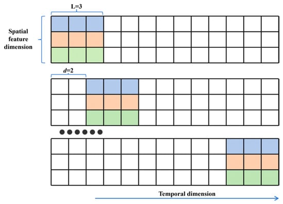
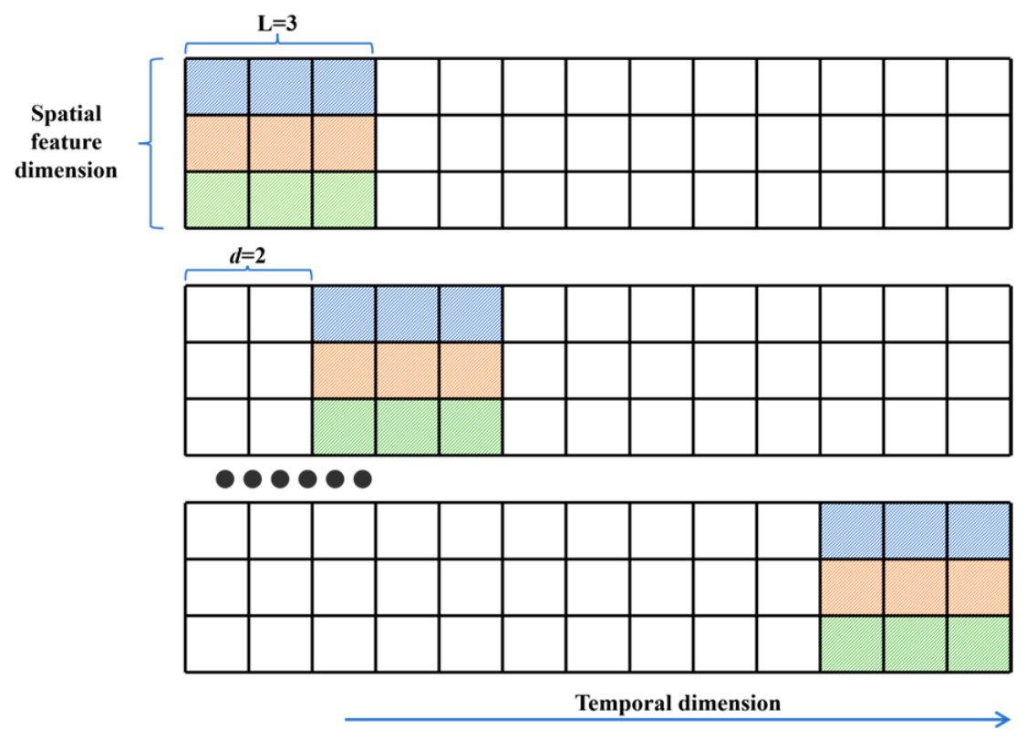
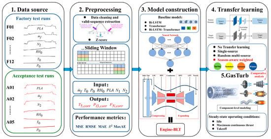
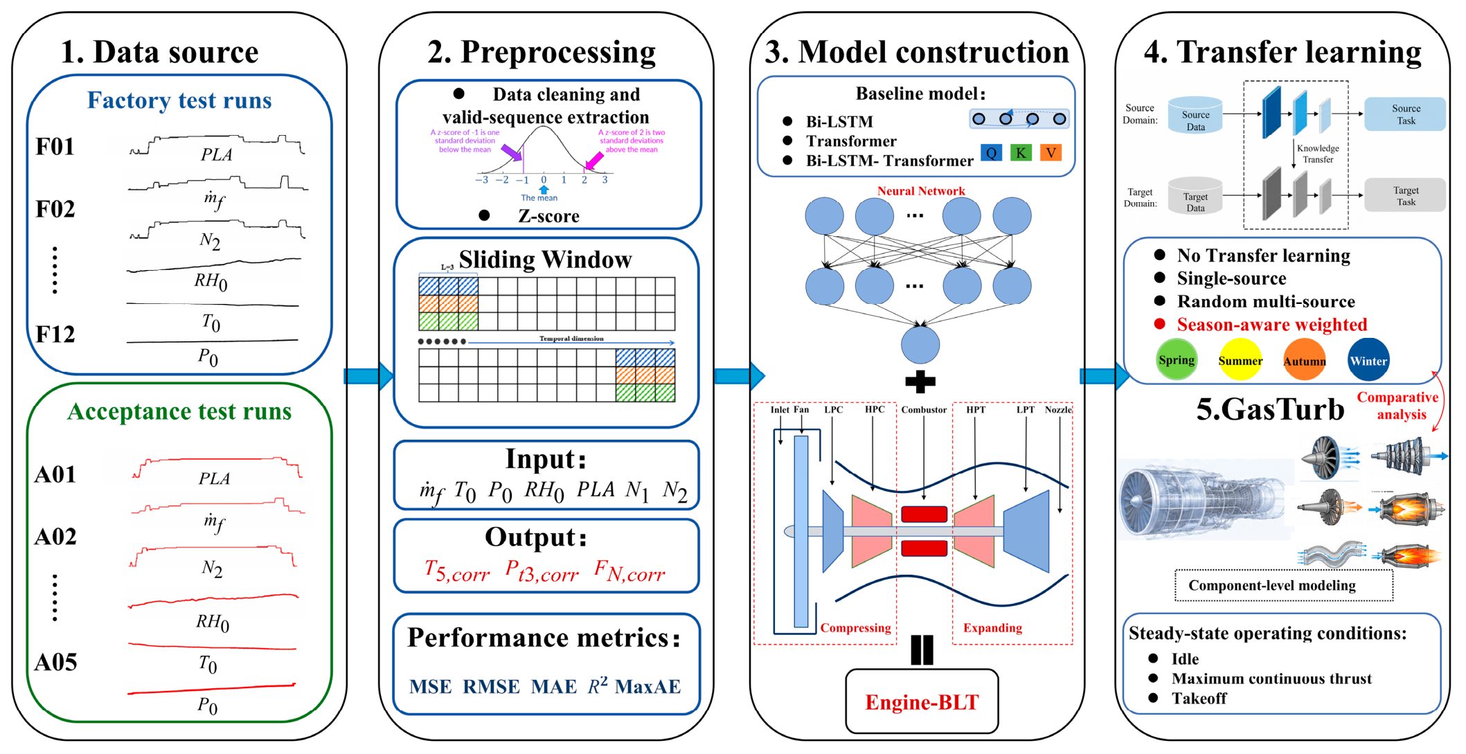
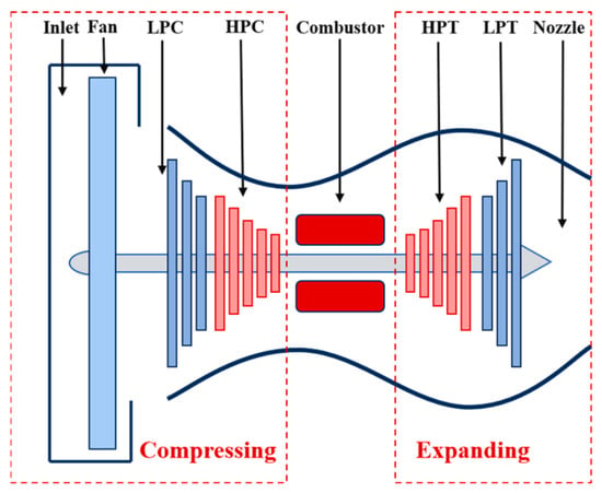
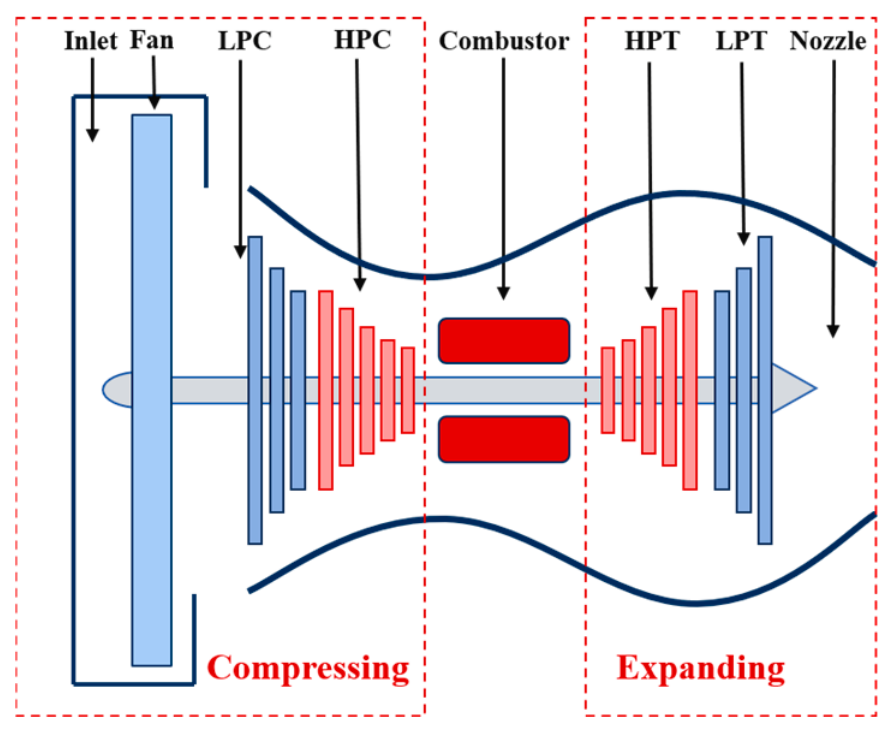
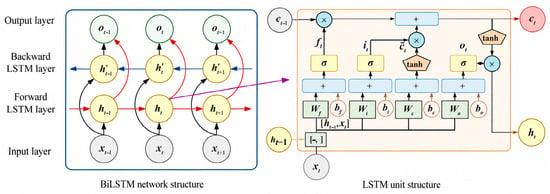
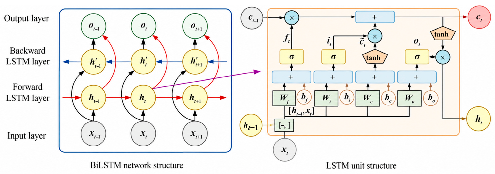
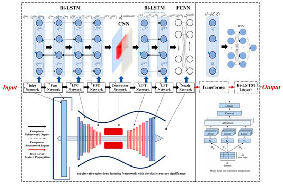
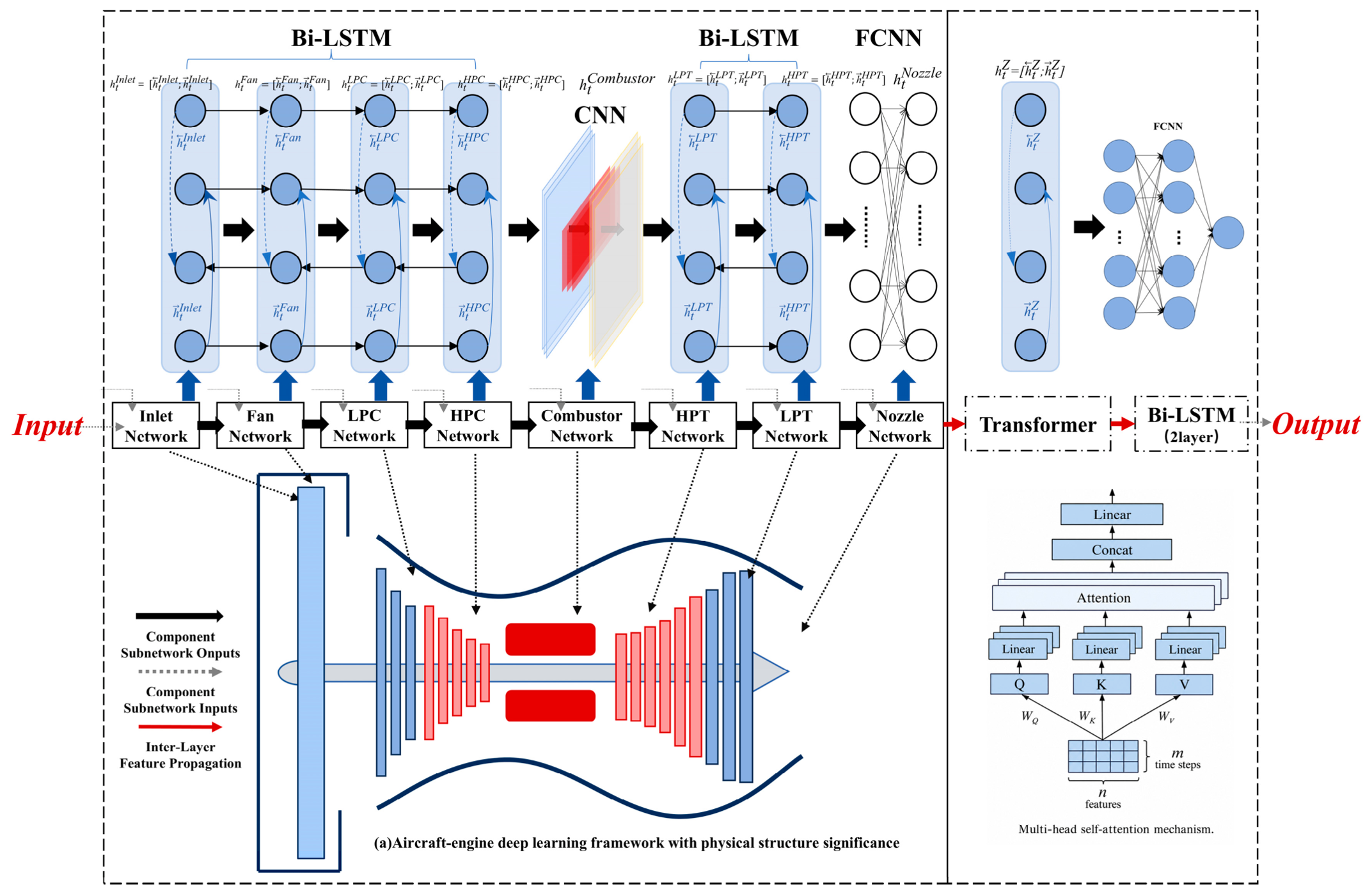
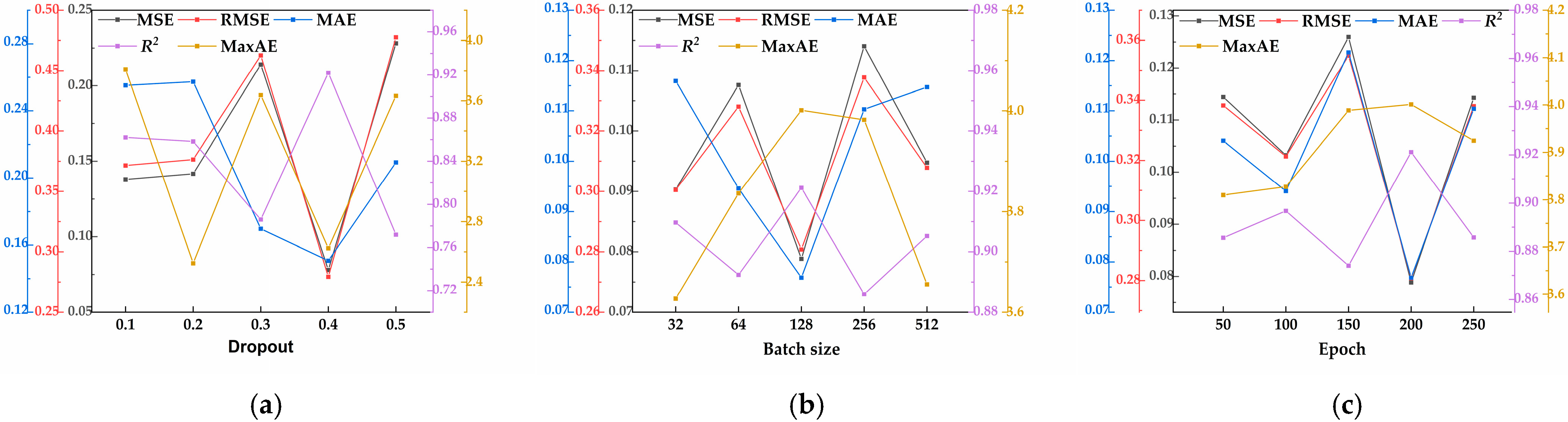
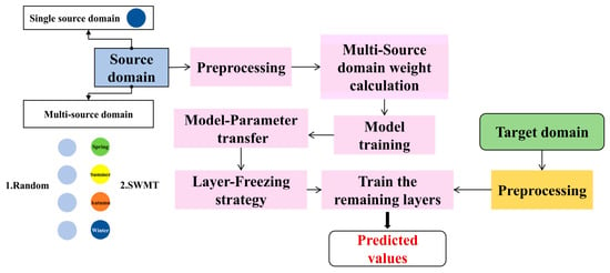
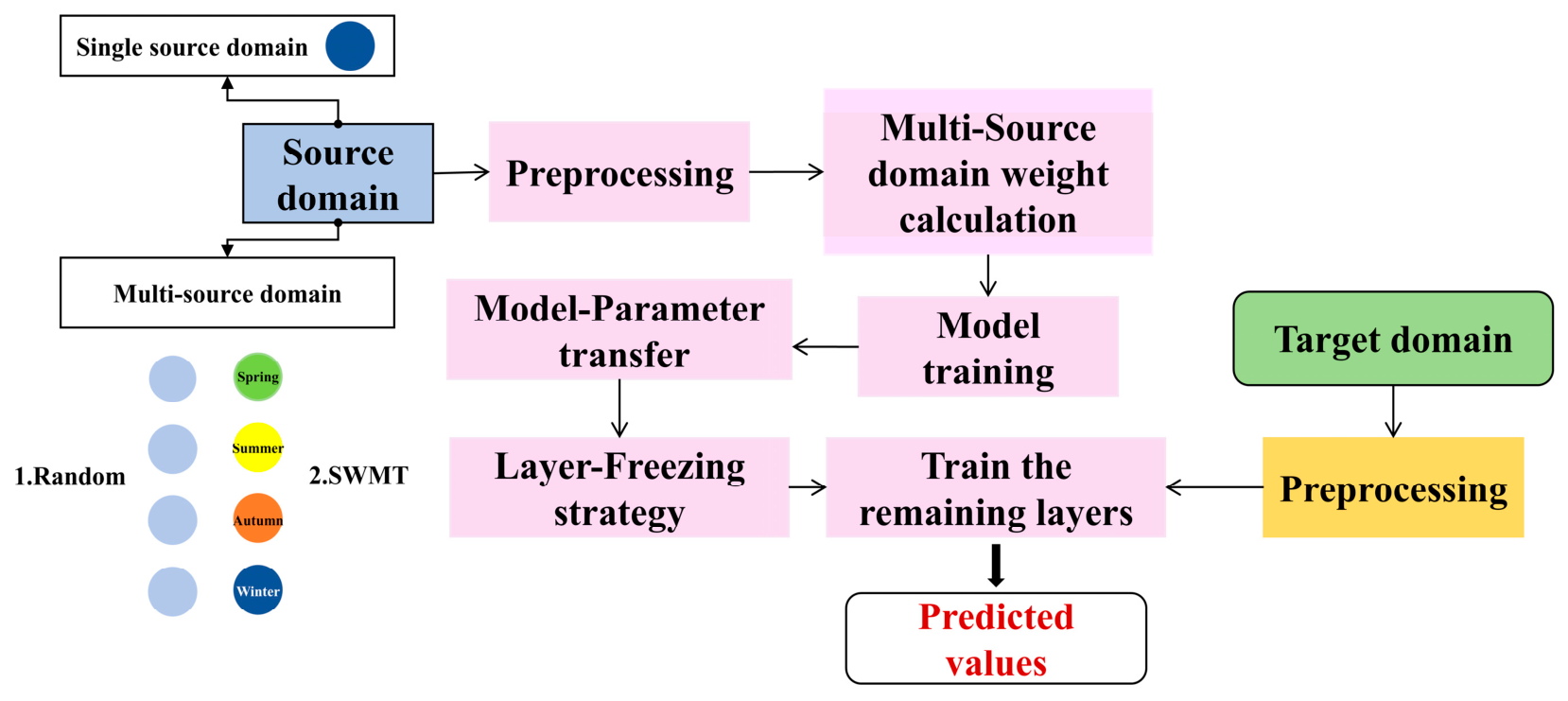
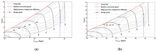
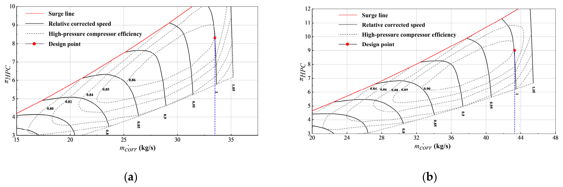
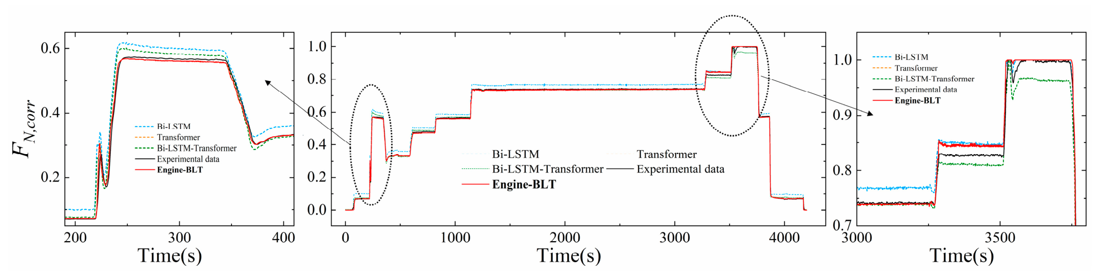
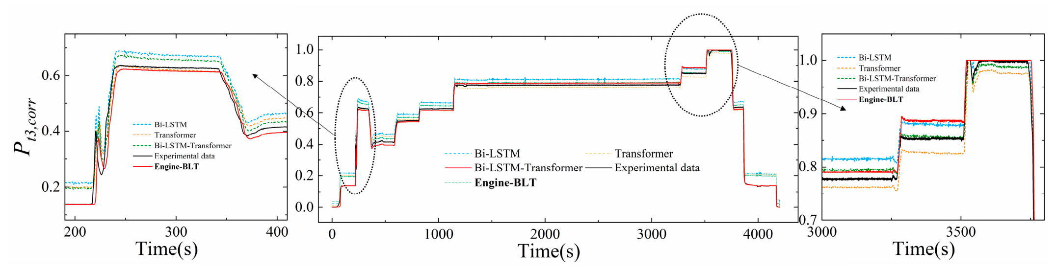
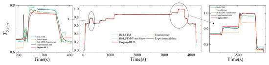
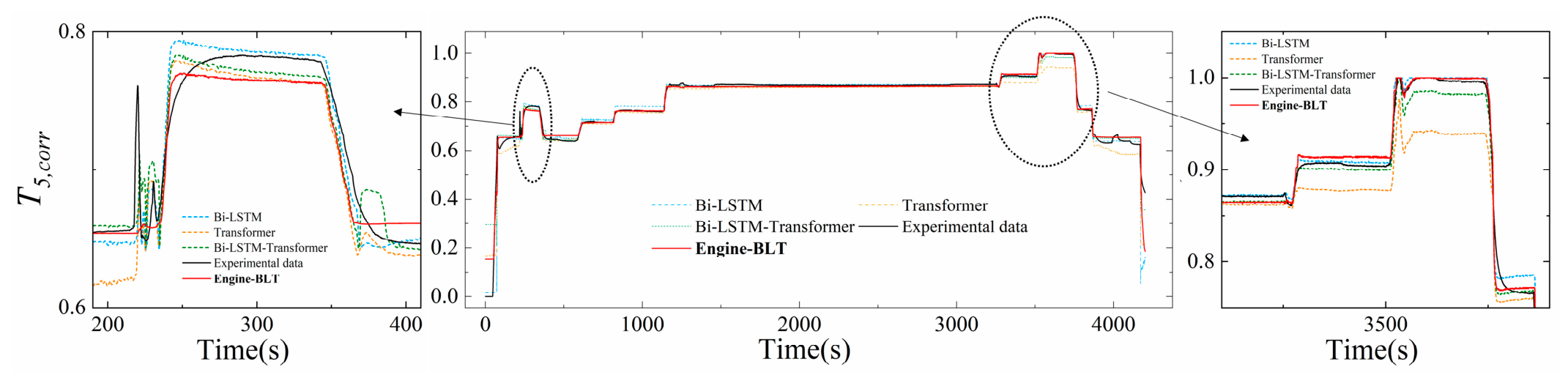
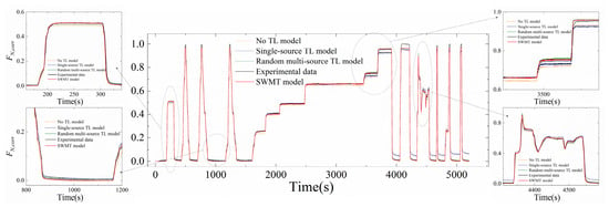
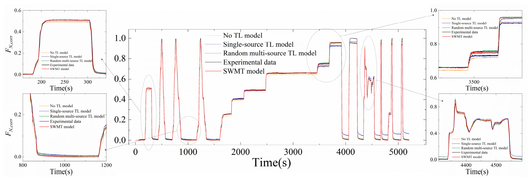
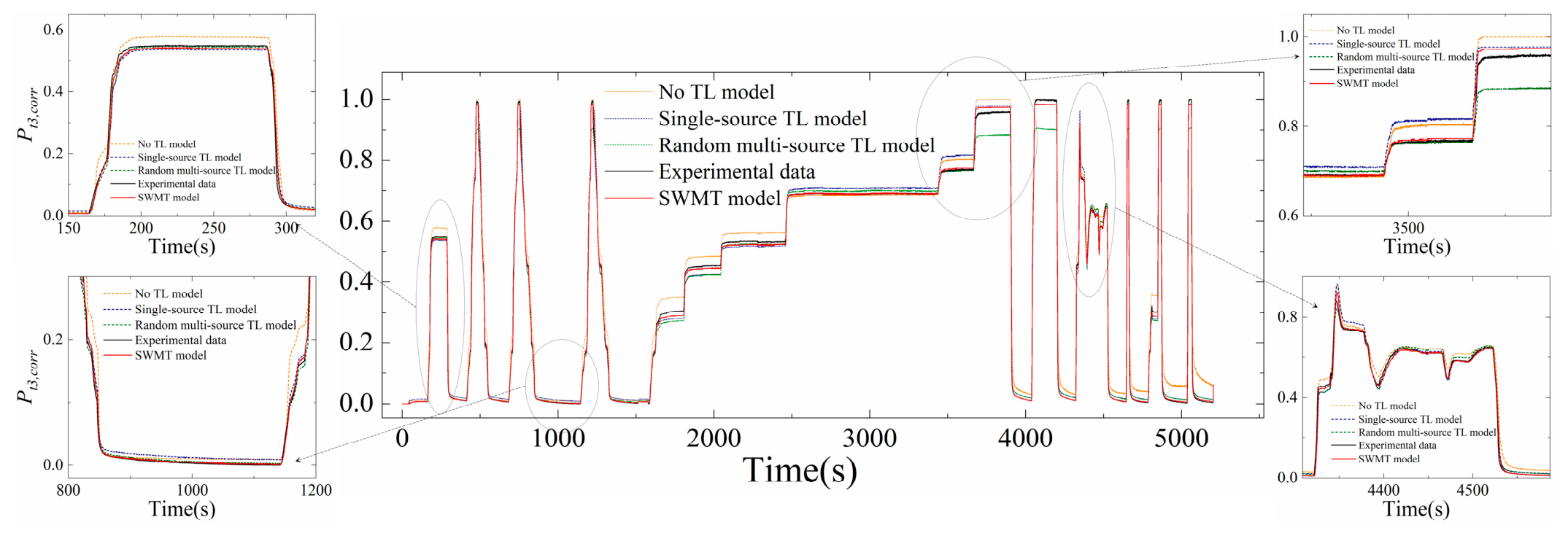
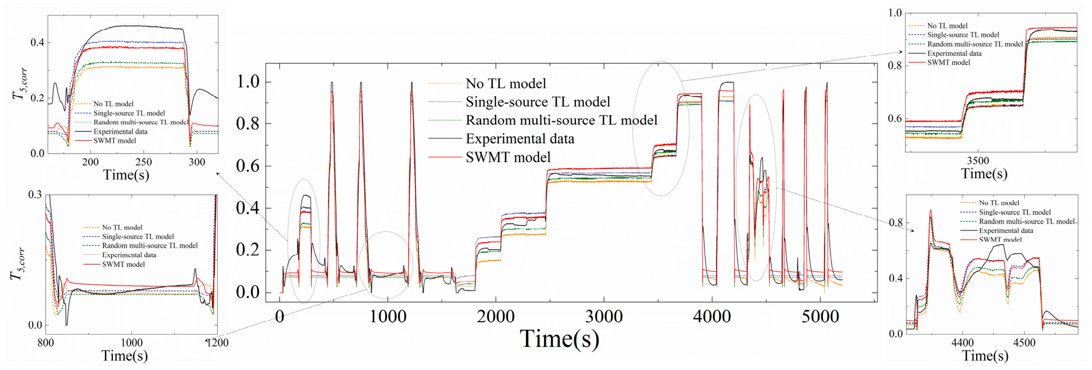
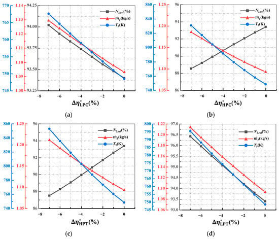
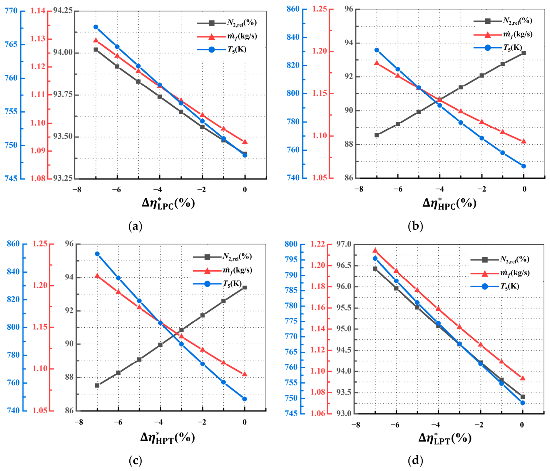

Disclaimer/Publisher’s Note: The statements, opinions and data contained in all publications are solely those of the individual author(s) and contributor(s) and not of MDPI and/or the editor(s). MDPI and/or the editor(s) disclaim responsibility for any injury to people or property resulting from any ideas, methods, instructions or products referred to in the content. |
© 2026 by the authors. Licensee MDPI, Basel, Switzerland. This article is an open access article distributed under the terms and conditions of the Creative Commons Attribution (CC BY) license.