


Abstract
Aircraft maintenance scheduling is a focus point for airlines. Maintenance is essential to ensure the airworthiness of aircraft, but it comes at the cost of rendering them unavailable for operations. In current operations, aircraft maintenance scheduling must often be updated to include time for non-routine (i.e., non-schedule) tasks. Non-routine maintenance tasks (NRTs) introduce significant uncertainty into aircraft maintenance scheduling, often leading to delays and increased operational costs. Despite their importance, limited research has been conducted on predicting NRT maintenance workload using data-driven methods. This study compares Random Forest and LGBM with a Weibull survival model for NRT workload prediction at the individual routine task (RT) level. Results indicate that model performance depends on data availability and the evaluation metric: using data from all tasks can help in sparse settings, while using an independent occurrence model to correct labor predictions may improve aggregate error at the cost of other outcomes. The historical-average baseline performed comparably to Independent LGBM on MAE, ROC-AUC, and average precision. Finally, results show that summing task-level predictions does not result into a good forecast for the work packages that contains all the tasks. Further data and prospective validation are needed before these estimates can guide work-package planning.
1. Introduction
Efficient scheduling and timely completion of aircraft maintenance are critical to the daily operations of airlines. Recent studies [1,2], and the Airline Maintenance Cost Executive Commentary [3], reveal that airlines allocate, on average, approximately 10% of their variable costs to maintenance. An effective maintenance schedule has two primary components: content and time. A more accurate estimation of the required duration for each time slot enhances the precision of maintenance task scheduling and reduces the risk of delays, thereby reducing the likelihood of Aircraft on Ground (AOG) events, which significantly disrupt airline operations. AOG incidents reduce profitability and increase maintenance costs [4].
The content of aircraft maintenance tasks typically consists of two categories: routine and NRTs. The former, RTs, are pre-defined activities outlined in maintenance manuals, which must be performed at regular intervals. These tasks are highly predictable, following a fixed schedule. In turn, NRTs encompass all unanticipated activities that may arise from various sources, such as wear-and-tear, system failures, or inspection findings. These tasks are the primary cause of maintenance delays and the main contributor to uncertainty in maintenance scheduling [5]. According to [6], non-routine work can take up 50% of the total maintenance completed during an aircraft scheduled service.
Accurately predicting the workload associated with NRTs is essential for effective maintenance planning, and airlines are increasingly recognizing its importance and seeking optimal solutions. Without predictive estimation, maintenance scheduling must either allocate excessive buffer time, leading to inefficiencies, or risk unexpected AOG situations. Recent investigations, including [7], have resorted to linear regression and supervised machine learning models for workload estimation based on historical data. However, the limited availability of data has resulted in inaccuracies and overfitting of supervised learning models. As mentioned in the research done by [7], data availability and confidentiality has delayed research in this area. The sensitive nature of these data means that only a select few airlines have access to means to work on this issue, further highlighting the significance and value of our research in this domain. Another challenge lies in the explainability of predictive methods. While machine learning has demonstrated strong potential in advancing predictive maintenance and fault diagnosis in aircraft maintenance, many of these models operate as ‘black boxes’, offering little insight into how decisions are made. This opacity can undermine trust and hinder adoption, particularly in safety-critical domains like aviation where transparency and interpretability are essential.
This paper compares survival analysis, Random Forest, and LGBM for NRT workload prediction using real-world data from a major European airline. The comparison is empirical and focuses on task-level predictions, with a analysis of work-package predictions. Our primary objective is to predict the duration (i.e., labor hours) of NRTs, which has a direct operational impact on aircraft ground time and scheduling buffers. NRTs often result in a delay of several hours, even lasting up to more than 5 h, potentially resulting in severe delays on flight operations. This prediction can be made at the time the RTs are planned, since all the necessary information is already available, including the aircraft’s flying hours and number of cycles at the time the RT is performed. Our framework is applied to real-world, 12-year proprietary airline dataset, specifically addressing the industry-wide challenge of zero-inflated, highly skewed maintenance data.
This paper is structured as follows. Section 2 provides more details on the nature of NRTs and the difficulties in its prediction. The current state-of-the-art on non-routine forecasting is defined in Section 3. Section 4 defines the different methods used for non-routine forecasting. The data and case study that these models are applied are defined in Section 5. Results of the data-based methods are presented in Section 7. Validation of these methods to a model-based methods is made in Section 8. The implications of the accuracy of the models and how these should be used by organizations are analyzed in Section 9. Finally, Section 10 concludes this work.
2. Problem Definition
The present section further elaborates on the definition of NRTs. Their source and occurrence are described in Section 2.1. The current approach by airlines to handle unexpected NR-labor hours is discussed in Section 2.2. Section 2.3 sheds light on the challenges in forecasting non-routine labor.
2.1. Definition and Source
Maintenance tasks can be classified into two primary categories: RTs and NRTs. The former are those that have been pre-scheduled, including those outlined in the maintenance program that must be executed regularly, as well as any other tasks planned in advance for various reasons, collectively referred to as preventive maintenance. The latter, on the other hand, encompass all unplanned maintenance activities that arise outside of the established schedule. These unexpected findings generate additional labor time and represent a specific subset of corrective maintenance. At the beginning of a shift, technicians typically focus on a list of RTs, while any additional maintenance requirements identified by either the technicians, the aircraft systems, or crew members are categorized as NRTs. Thus, three different sources of NRTs are defined:
- Arising from RTs: While technicians conduct pre-scheduled RTs, they may encounter additional issues that require attention. These NRTs are often related to the RTs from which they originate. This constitutes the primary source of NRTs. The remaining records arise from two additional sources, which are detailed in the following paragraphs.
- Identified during WPs: Work package is a list of RTs and NRTs that need to be carried out at one maintenance slot. Technicians working on specific WPs may discover maintenance needs that are not directly linked to scheduled RTs. For example, a technician might notice a dent in an aircraft while performing a routine inspection, which is not part of the pre-defined maintenance checklist for that work package.
- Reported by aircraft systems or crew members: NRTs may also be identified by the aircraft’s systems or reported by crew members during operations, such as a crooked screw on the aircraft seats due to misuse.
Note that this study focuses on predicting NRTs arising from RTs. NRTs reported independently by aircraft systems or crew members (Source 3) are outside the fitted RT-level target. The source-link audit and independent-source counts are reported in the Case Study; because they use different classifications, they are not treated as interchangeable. A direct analysis of their transmission into WP-level error remains future work.
2.2. Current Industry Approach
Given the difficulty in predicting exact non-routine labor hours, and the economical consequences of grounding an aircraft [8], to accommodate NRTs, airlines typically insert time buffers into the maintenance schedule. However, these time buffers are often based on heuristic estimations, utilizing either a fixed percentage of the expected RT duration or an arbitrary fixed time value [9,10]. Because these static buffers fail to capture true operational variance, they often result in overly conservative schedules that waste aircraft availability. Conversely, advanced scheduling literature suggests that more accurate time buffers can be calculated by assuming that maintenance task uncertainties follow a statistical probability distribution [11,12], allowing for dynamic buffer sizing that minimizes both schedule risk and aircraft downtime. The airlines decides which quantile of the distribution to consider. Selecting a higher quantile results in a more conservative approach, where additional time is allocated for maintenance tasks.
As described in [13], other proactive approaches include the design of robust scheduling that allows convenient alternatives in regards to flights, aircraft, and crews to reduce the impact of disturbances in the maintenance plan. However, on the scale of large airlines, such is not always possible. Additionally, often, maintenance and networking planning are decoupled decisions. The complexity of dynamic scheduling of flight and crew is not trivial. While dynamic, operational adjustments to crew pairings are highly prevalent in daily airline operations, minimizing disruptions to the baseline schedule remains a primary objective for airlines.
2.3. Challenges on Non-Routine Labor Forecasting
Several challenges must be addressed to understand the complexities surrounding the prediction of non-routine maintenance tasks. First, some RTs occur only at extended intervals, limiting available data for these tasks. While ample data exists for frequently performed tasks, less frequent tasks suffer from data insufficiency. Second, some NRTs are inherently unpredictable, as they often arise spontaneously without prior indicators. For instance, replacing an expired component constitutes a non-routine maintenance task. Repairing an overused and damaged seat also falls under non-routine maintenance. However, predicting when the seat will fail is challenging due to the numerous factors influencing its deterioration. This randomness complicates the ability to forecast certain types of non-routine.
Additionally, each NRT is almost entirely distinct, and while some tasks may show similarities, they are rarely identical. For example, repairing a broken screw is a non-routine maintenance task involving mechanical repair, whereas restocking printing paper, though vastly different in nature, is also considered non-routine. Despite their differences, both tasks fall outside the scope of regular scheduled maintenance. This uniqueness further complicates predictive modeling efforts.
Finally, in the specific case of data-based forecasting models, having data that contain an abundance of zero values is commonly known as zero-inflation [14], which can introduce prediction bias, leading the model to overpredict zero values. This is the case with this dataset, where most RTs have zero NRTs.
Given these challenges, it is clear that predicting NRTs varies significantly across different cases. A single, generalized model may not yield optimal results. Instead, distinct predictive approaches are required for each source of NRTs, which adds complexity to the overall problem-solving process.
3. Literature Review
The present section covers the state-of-the-art on multiple sources. Section 3.1 covers the existing limited work on NRT prediction. Section 3.2 expands on the work directed at predictive maintenance, highlighting the importance of predicting maintenance labor. Finally, Section 3.3 will focus on forecasting methods across all disciplines.
3.1. Predicting Non-Routine Aircraft Maintenance Workload
Research on non-routine aircraft maintenance workload remains highly limited. Ref. [6] was among the first to address the issue by focusing on reducing NRTs rather than predicting them, achieving a reduction of over 50% in such tasks. Ref. [15] attempted to predict non-routine workload using Bayesian inference and Markov Chain Monte Carlo methods. Similarly, ref. [7] explored data-driven algorithms for workload prediction, demonstrating significant improvements. Ref. [16] applied supervised learning techniques to predict non-routine workload, also reporting notable advancements.
Beyond workload prediction, some studies have investigated the prediction of materials required for non-routine maintenance. Ref. [17] employed multiple models to forecast material needs for NRTs. However, due to data quality limitations and the complexity of the problem, the predictive models, while showing some degree of accuracy, remain insufficiently reliable for real-world implementation.
3.2. Related Research in Predictive Maintenance
Although research in aircraft maintenance workload prediction is scarce, numerous studies have applied data-driven techniques to predict various outcomes. Non-routine workload prediction shares similarities with several well-established academic problems. It can be modeled as a workload prediction problem [18,19,20], or as a failure prediction problem or as known as remaining useful life (RUL) prediction [1,21,22,23,24,25]. While these studies may not provide direct solutions to our problem, their methodologies offer valuable insights for selecting suitable approaches. The former group, workload prediction, provides insights on how to model dynamic and uncertain workloads using historical system data, as demonstrated by [18], who used Autoregressive Integrated Moving Average to forecast cloud Virtual Machine usage, and by [20], who proposed a compact and efficient deep learning architecture for time-series workload prediction [20]. Ref. [19] further contributed by incorporating predictive uncertainty using Bayesian deep learning to better plan for fluctuations in industrial production systems.
The latter group, failure prediction, offers strategies that translate well into aircraft maintenance forecasting. Ref. [1] used SV to estimate the time from alarm to failure, enhancing alarm-based maintenance decisions. Ref. [21] proposed a Poly-Cell LSTM to forecast the remaining useful life (RUL) of lithium-ion batteries by dynamically weighting feature importance. Ref. [22] introduced a Transformer-based multi-task learning model with boosting to predict aero-engine RUL under varying operating conditions. Ref. [23] developed a hybrid CNN-LSTM model to jointly optimize RUL prediction and imperfect maintenance scheduling. Ref. [24] designed a lightweight dual-attention LSTM architecture with exponential smoothing to improve RUL estimation efficiency. Finally, ref. [25] created a CNN-BiLSTM ensemble for accurate RUL forecasting, which feeds into a dynamic predictive maintenance strategy to optimize operational decisions.
3.3. Approaches for Forecasting
This section will give an overview of the current state-of-the-art for forecasting methods. Section 3.3.1 will focus on traditional data-based methods. In turn, Section 3.3.2 introduces recent efforts on supervised learning.
3.3.1. Model-Based Approaches for Forecasting
Model-based methods aim to establish mathematical or physical models to characterize the degradation processes of machinery, with model parameters updated using measured data [26,27]. Commonly employed models include the Markov process model [28,29], the Wiener process model [30,31,32], and the Gaussian mixture model [33,34]. These methods integrate both expert knowledge and real-time data from machinery, making them particularly effective for RUL prediction (i.e., the remaining time before system health falls below a pre-defined threshold).
Specifically, SV is a statistical technique for analyzing time-to-event data, commonly used to predict failure times, machine breakdowns, and other duration-based outcomes. Unlike traditional regression models, SV accounts for censored data, where the exact event time is unknown for some subjects. Ref. [35] applied SV to develop failure prediction models and estimate lifespans in duration-based scenarios. Ref. [36] examined the applicability of SV in bankruptcy prediction, demonstrating its ability to assess risk over time while handling censored data. Recently, ref. [37] proposed a novel machine failure prediction model that integrates machine learning and SV to improve prediction accuracy. Ref. [32] develops a survival-analysis based PdM strategy for hard failures. Finally, ref. [38] defends that SV results can be incorporated into actual predictive maintenance applications in the future.
3.3.2. Supervised Learning Approaches for Forecasting
Data-driven methods [39] have gained significant attention in predictive maintenance due to their ability to model complex relationships in large datasets without requiring explicit physical degradation models. These methods leverage historical and real-time data to identify patterns and predict maintenance needs with high accuracy. Compared to traditional model-based approaches, data-driven techniques can adapt to various operational conditions and improve prediction robustness.
RF [40], an ensemble method that constructs multiple decision trees, has been extensively applied in aircraft maintenance prediction. Ref. [41] utilized it to assess the significance of historical engine monitoring parameters, identifying features (specifically flight cycles, flight hours, and historical records) that influence engine lifetime. Ref. [42] proposed an improved artificial fish-swarm optimization stochastic forest algorithm to enhance engine delivery grade classification. Ref. [43] integrated sensor and environmental data using RF to estimate RUL. Ref. [44] applied RF for engine rotor fault diagnosis, comparing its performance with support vector machines.
Boosting, an ensemble learning technique that enhances weak learners (typically decision trees) by sequentially improving their predictive performance, has been widely applied in aircraft maintenance, particularly in predicting the remaining useful life (RUL) of components. Ref. [45] employed XGBoost [46] to develop an AI-driven predictor for aircraft engine RUL. Ref. [47] utilized the LGBM [48] algorithm on NASA-provided datasets, incorporating time-windowed data and engine runtime as predictive features. Ref. [49] explored multiple predictive models, demonstrating that boosting methods significantly enhance maintenance requirement accuracy. Ref. [22] addresses aero-engine RUL prediction under cross-domain (working-condition) changes using a multi-task learning and boosting approach.
In addition to these approaches, other machine learning methods have also been applied to forecasting and predictive maintenance. Artificial neural networks have been utilized for failure prediction tasks due to their ability to capture complex nonlinear patterns in sensor and operational data [50,51,52,53,54]. LSTM (Long Short-Term Memory) networks are commonly used in maintenance prediction due to their ability to model complex temporal dependencies and trends in compartment failure data [55,56,57,58]. Similarly, support vector machines have been employed for their effectiveness in high-dimensional classification problems, making them suitable for identifying early signs of failure in various industrial systems [59,60].
4. Methodology
The present study makes a direct comparison between multiple forecasting methods. The main objective is to directly compare model and data-based methods for the specific case of non-routine labor hours prediction. Since this case falls within the domain of aircraft maintenance, where safety and reliability are paramount, even a highly accurate black-box model may be unsuitable if its results cannot be clearly understood or explained by technicians. Trust in the output is essential for practical use. Therefore, in this study, we selected forecasting methods for comparative predictive evaluation and practical implementation: Random Forest, LGBM, and SV.
First, Section 4.1 explains the developed framework, where our prediction model is used to predict the NRT labor hours for a scheduled RT. Second, Section 4 covers the high level approach of this forecasting. Finally, Section 4.2 provides an overview of the fundamental principles of SV and outlines the rationale for selecting this approach. In Section 4.3, we present the theoretical foundations of LGBM and Random Forest, highlighting their distinctive characteristics and the justification for their selection in this study.
4.1. NRTs Forecasting for Each RT
We estimate NRT labor hours and evaluate the trade-off between occurrence detection and labor error. The Sequential model first predicts the NR count; a count of at least 0.5 defines the binary occurrence output, and chronological out-of-fold predicted NR counts enter a labor regressor trained on all training rows of data. The Filtering model predicts an occurrence probability with a classifier and thresholds it at 0.5, fits the labor regressor independently on all rows and the same stage-specific input matrix, and applies the binary occurrence decision only at evaluation. Neither regressor is trained only on positive cases. The resulting data flow is illustrated in Figure 1; for consistency with the figure artwork, SEQ means Sequential model and FIL means Filtering model.
Figure 1.
Visual representation of the Sequential model and Filtering model. The two branches of the Filtering model—the occurrence classifier and labor hour regressor—are fitted independently in parallel on the same training rows and features, and are combined only at evaluation by hard gating: predicted occurrence zero yields zero labor hours, whereas predicted occurrence one retains the labor prediction.
The Random Forest and Light Gradient Boosting Machine models use six common predictors: flight cycles, flight hours, the NR-labor hours observed during the two most recent executions, and the numbers of NR tasks observed during those executions. In the unified approach, one model is trained using data from all RT types, and an encoded RT-Code is included to distinguish them. In the individual approach, a separate model is trained for each RT-Code, so RT-Code is used only to divide the data and is not included as a predictor. In the sequential pipeline, the predicted number of NR tasks is added as an input to the labor hour model. In the filtering pipeline, the occurrence and labor models are fitted independently; the occurrence prediction is used only at evaluation to set the reported labor prediction to zero when no NR task is predicted.
4.2. Model-Based Method (Emphasis on SV)
SV [61] models the time to an event and can use censored observations for which a subsequent event is not observed. In this study, a survival observation is a repeated execution of one specific inspection task. The event is the occurrence of a non-routine fault, and time is measured as the number of scheduled checks since the previous fault. The clock therefore resets after every observed fault.
Aircraft entry into airline service defines the observation-window origin. The first interval is treated as uncensored when the aircraft is new and is followed from service entry. When prior maintenance is unknown, the first observed interval is only a lower bound on the elapsed time and contributes a survivor term rather than a failure-density term. Repeated fault gaps are retained as intervals in a Weibull fit for each task. The final 50 work packages are excluded from Weibull fitting and model selection and are used only for the test predictions.
Its ability to estimate the probability of failure over time provides essential insights into failure patterns and component longevity, with the Weibull distribution being a popular choice for capturing varying hazard rates. The Weibull distribution is governed by two fundamental parameters: the shape parameter k and the scale parameter . The shape parameter k determines how the hazard rate evolves over time, while the scale parameter defines the characteristic time of the process. The Probability Density Function (PDF) of the Weibull distribution is expressed as
One of the most compelling aspects of the Weibull model is its ability to represent different failure mechanisms through variations in the shape parameter. When , the hazard rate decreases over time, capturing early-life failures that are often seen in reliability engineering. In contrast, if , the hazard rate remains constant, reducing the Weibull distribution to an exponential model that is commonly used to describe random failures. Finally, when , the hazard rate increases with time, reflecting aging-related failures, which are an essential characteristic for modeling wear and tear in mechanical systems or disease progression in medical studies.The hazard function, which describes the instantaneous failure rate at a given time, is given by
To estimate k and , we use maximum likelihood with the censoring indicator , where for an observed fault and for a censored interval. With survivor function , the likelihood is
This form includes observed fault gaps and censored lower bounds. The available materials describe task-specific recurrent gaps, but do not document how within-aircraft dependence was handled. Frailty or clustered recurrent-event terms are therefore future-work extensions rather than claims about the closed implementation.
The implemented SV labor prediction multiplies the saved occurrence probability, denoted by , by the per-RT-code mean of prior positive NR labor hours, using all available history before each package cutoff and the pooled positive-training mean as a fallback when no task-specific history is available. Specifically, the prediction satisfies
where is the corresponding historical mean NR labor value. The binary occurrence field equals one when the predicted labor exceeds 0.166 person-hours, approximately 10 min.
4.3. Supervised Learning Algorithms
Data-driven methods offer significant advantages over model-based approaches when sufficient data is available. These methods, particularly machine learning algorithms, leverage large datasets to uncover complex patterns and relationships without the need for explicitly defined physical models. This makes them highly adaptable and effective in situations where the underlying system dynamics are too complex or unknown to model directly.
In our case, RF and LGBM were selected for their strong performance in handling complex, high-dimensional data with minimal parameter tuning. RF’s ensemble approach allows for robust, accurate predictions by combining multiple decision trees, while LGBM excels in handling large datasets efficiently, providing fast and scalable learning for predictive maintenance tasks.
4.3.1. Random Forest (RF)
Random Forest (RF) is used in this study for both stages of the forecasting framework: (i) NRT occurrence classification and (ii) NRT labor hour regression. RF is selected because it captures nonlinear interactions, is robust to noisy maintenance records, and performs well under moderate feature dimensionality.
Given a training set , RF builds K trees on bootstrapped samples :
At each node split, RF considers only a random subset of features, which decorrelates trees and improves generalization.
For the occurrence stage (), each tree outputs a class vote. The forest-level class is obtained by majority vote:
The occurrence probability can also be interpreted as the fraction of trees voting for class 1:
The two RF variants use occurrence information differently. In the sequential variant, the RF labor hour regressor is trained on all training rows and receives the chronological out-of-fold predicted NR count as an additional feature. It predicts labor hours directly at evaluation, with no hard-zero step. In the filtering variant, the occurrence classifier and labor hour regressor are fitted independently on all rows and original features. At evaluation, the independent labor prediction is multiplied by the binary occurrence decision:
where comes from a regressor trained on all rows. Filtering changes the evaluation output, not the regressor’s training sample.
For these zero-inflated data, sequential prediction keeps the continuous labor estimate and uses chronological occurrence information. Filtering imposes the occurrence decision at evaluation, trading recall and positive-case accuracy for lower overall MAE.
Table 1 lists the fixed RF settings used in the robustness analysis.
Table 1.
Hyperparameter configurations for RF models.
4.3.2. Light Gradient Boosting Method (LGBM)
Light Gradient Boosting Machine (LGBM) [48] is the second data-driven algorithm used for both tasks in our framework (occurrence classification and NRT labor hour regression). LGBM is suitable for this study because it combines high predictive power with efficient training on large maintenance logs.
LGBM builds an additive ensemble of trees by minimizing a task-specific loss:
where is the tree fitted at iteration t and is the learning rate. In each boosting round, the new tree is fitted to current residual errors, so subsequent trees correct the mistakes of earlier ones.
For occurrence classification, LGBM optimizes a binary objective. The model outputs a score , converted to probability through a logistic link:
A threshold then provides the binary decision .
LGBM uses the same two variants. In the sequential variant, the labor hour regressor is trained on all rows with the chronological out-of-fold predicted NR count as an additional feature. Its evaluation predictions are not set to zero. In the filtering variant, the occurrence classifier and labor hour regressor are fitted independently on all rows and original features. The evaluation-time labor prediction is then multiplied by the binary occurrence decision:
Here, comes from a regressor trained on all rows; filtering does not restrict the training sample.
Its practical efficiency comes from three design choices: (i) histogram-based split finding, which discretizes continuous features into bins; (ii) leaf-wise growth, which expands the leaf with the largest loss reduction; and (iii) gradient-focused sampling, which prioritizes high-information observations. These mechanisms reduce runtime and memory use while preserving accuracy.
Table 2 reports the fixed LGBM settings used in the robustness analysis. We fixed them before evaluating the test set.
Table 2.
Hyperparameter configurations for LGBM models
We use Unified model for a unified RT model trained across RT codes, Independent model for separate models trained per RT code, Sequential model for the sequential labor pipeline, and Filtering model for the filtering labor pipeline.
4.3.3. Input Features
Table 3 lists the features actually supplied to the RF and LGBM models in the retained robustness analysis. Each modeling row represents one unique RT barcode. The six base features use the original labels shown in the feature-importance figures. RT-Code is added only to Unified models, and the predicted NR-task number is added only to Sequential model labor stages. Execution and package keys and aircraft registration are used for joins, deduplication, package-level splitting, and same-aircraft histories; they are not fitted predictors.
Table 3.
Input features actually supplied to the retained RF/LGBM models.
Scheduled labor, realized start and end times, current NR outcomes, and current-package records are not fitted predictors. Timestamps only order completed history and define the retrospective cutoff. Records from the package being predicted are excluded when its historical features are constructed, preventing within-package leakage.
The WP barcode assigns each row to a work package (WP) for package-level splitting and aggregation. Fly Cycles and Fly Hours are planning-time predictors of operational exposure.
Current NR count and current NR person-hours are prediction targets. The binary occurrence label is derived from the current NR count and is positive when the count is non-zero. The lagged features use only the two most recent completed NR-count and NR-labor values for the same RT code and aircraft. Multiple matched NR records are summed before the current count and labor targets are formed, and an unavailable history value at the cutoff is filled with zero.
5. Case Study
The dataset utilized in this study comprises maintenance records from a major European airline, encompassing a fleet of 31 aircraft over nearly 12 years, from October 2012 to July 2024. The raw archive contains 540,394 RT/task rows, 4993 RT codes, 2194 work packages, and 94,946 NR records. The analysis is retrospective and the test set was fixed before the robustness run; it is not a prospective deployment evaluation.
In this airline’s maintenance operations, the set of tasks performed during each maintenance event is referred to as a work package (WP). Each WP consists of multiple RTs (RTs) and NRTs (NRTs). The supplied test data contain 18,362 raw RT rows from 50 work packages. After deduplication, the modeling test set contains 16,652 unique RT barcodes and 1268 RT codes; the modeling table has one row per unique RT barcode. Duplicate raw records account for the difference in row counts. Table 4 reconciles these data stages, and Table 5 gives the split for the chronological robustness analysis.
Table 4.
Compact reconciliation of the archive and fixed test set.
Table 5.
Chronological split used for the robustness analysis.
The experiment’s predictions cover the same 16,652 valid test rows, 1268 RT codes, and 50 work packages. We analyze these predictions separately, using fixed specifications and package-frozen histories without tuning on test outcomes. Among all 94,946 NR records, 92,876 are coming from RT (97.820%). The other sources account for 2.178% of the records. Table 6 summarizes how often each RT was performed in the archive.
Table 6.
Number times that the RTs (RTs) were performed.
In the final modeling test set, 1716 of 16,652 tasks have a non-zero occurrence target and 1650 have positive capped labor. Table 7 uses these denominators and reports non-overlapping occurrence and labor categories.
Table 7.
Occurrence and labor outcomes in the 16,652-row modeling test set.
Additionally, a distribution of RTs included in each WP is shown in Table 8. In the fixed test set, package size ranges from 301 to 436 RT rows (mean 367.24; median 369), so aggregation is evaluated at package level but is not treated as an independent row-level replication.
Table 8.
Number of RTs (RTs) per work package (WP).
Repeating the analysis with uncapped labor values produced only negligible changes in task- and package-level MAE and did not alter the substantive conclusions, so the 24-person-hour cap was retained as a documented preprocessing choice.
6. Hypotheses
In this section, we present the hypotheses regarding the different models’ performance in terms of non-routine labor prediction. Note that in this work, two building steps are performed in order to establish the bet forecast method given the availability of the data. First, we determine the best framework for data-based methods. The corresponding hypotheses are described in Section 6.1. Second, comparison is done with a model-based method that assumes a pre-defined distribution. The hypotheses for this comparison based on the properties of the NRT are elaborated in Section 6.2. Finally, Section 6.3 covers the expected efficiency of using non-routine estimation over a work package with multiple RTs.
6.1. Hypotheses on the Performance of Data-Based Methods
With data-based methods, the main question is whether to have forecast methods per RT or to have one global model, taking the specific RT as input. Such depends on how similar the RTs are and whether a general feature pattern is applicable to the majority of the RTs. Additionally, when a global approach is used, the data for all RTs may be used. This is positive for RTs with little data. However, for other RTs, where more information is available, the agglomerations with others RTs may be negative in case its occurrence behavior differs from the norm. As it was observed in Section 5 that there is limited data, we formulate the following hypothesis:
Hypothesis 1.
A unified model that uses all routine task data to determine non-routine labor hour is more effective than constructing separate models for each RT.
Additionally, note that, in Section 5, two different values are available in terms of non-routine workload: the occurrence of NRTs and total number of non-routine labor hours resulting of each RTs. As previously mention in Section 2.3, zero-inflation can hinder the accuracy of forecasting methods. In this zero-dominated setting, applying an occurrence decision may lower overall MAE while worsening other outcomes. We therefore test occurrence filtering while also evaluating recall, positive-case accuracy, bias, and work-package performance.
Hypothesis 2.
We test whether occurrence filtering lowers overall MAE in zero-dominated data while considering recall, positive-case accuracy, bias, and work-package performance; no universal improvement is assumed.
6.2. Hypotheses on Data vs. Model-Based Methods
In this work, we make a differentiation between data-based, i.e., RF and LGBM, and model-based, i.e., SV methods. The latter assumes that NRT occurrence will follow a Weibull distribution. In turn, data-based methods make no such assumption. These use the input features to establish relational patterns between the input features. RF and LGBM are expected to better understand the pattern of NRT occurrence as long as sufficient data is available. Following, the hypotheses of this work are defined:
Hypothesis 3.
The data-based algorithms, namely RF and LGBM, are expected to outperform the SV when a sufficient amount of data is available. Note that what sufficient entails will be evaluated in Section 7.
Hypothesis 4.
In continuation from Hypotheses 3, it is expected that the SV method will be a better option for predicting non-routine labor for RTs with little data, as it is expected that data-based methods will not be able to find a pattern in such cases.
6.3. Hypotheses on the Prediction of NRT for WPs
We also aim to investigate how to generate accurate total work-package predictions based on the available task-level predictions, as the WP represents the most practical and straightforward unit for planners and technicians. The following hypothesis is formulated based on our RT-level prediction approach:
Hypothesis 5.
Aggregating individual RT-level non-routine labor predictions improves work-package-level forecasting accuracy relative to a historical-average work-package baseline, defined as the mean labor of historical work packages.
7. Results
We compare the data-driven models using separate occurrence and labor metrics. Occurrence is a binary outcome; labor is measured in capped person-hours. We report several classification metrics for occurrence and use overall MAE, positive-case MAE, bias, and underprediction for labor. Section 7.1 and Section 7.2 report the predictions and the chronological analysis separately. The architecture and pipeline comparisons follow in Section 7.3 and Section 7.4, with an RF/LGBM summary in Section 7.5 and feature-importance results in Section 7.6.
7.1. Primary Results Analysis
Table 9 gives occurrence metrics and work-package-cluster bootstrap 95% intervals. Labor metrics are reported separately because the target is zero-inflated.
Table 9.
Primary occurrence results. Intervals are work-package-cluster bootstrap 95% intervals.
The labor predictions reveal a similar trade-off. Under the Sequential model, row-weighted MAE is 0.2776 h for the Unified model using RF, 0.2988 for the Independent model using RF, 0.2885 for the Unified model using LGBM, and 0.3202 for the Independent model using LGBM. The Filtering model reduces these values to 0.2530, 0.2668, 0.2398, and 0.2532 h, respectively. The supplementary audit table reports the corresponding cluster-bootstrap intervals. The Filtering model is not uniformly better: in the predictions, it increases negative bias and can worsen error for positive-labor cases.
7.2. Chronological Robustness Analysis
The analysis uses the temporal split in Table 5, package-frozen histories, and chronological out-of-fold first-stage predictions for the sequential labor models. The historical-average task baseline predicts labor using the historical mean for each RT code. Table 10 reports classification, labor, and baseline metrics for the fixed 16,652-row test set. “Under” is the share of rows in which predicted labor is below actual labor; positive MAE uses only rows with positive actual labor.
Table 10.
Chronological robustness results on the fixed test set. Labor values are capped technician person-hours.
The historical-average baseline performed comparably to Independent LGBM on MAE (0.2825 vs. 0.2973 h), ROC-AUC (87.24% vs. 86.36%), and average precision (48.27% vs. 48.25%). Independent LGBM improves positive-case detection (F1 46.97% vs. 38.69% for the historical-average baseline and 0% for always-zero) and has less negative signed bias (−0.0136 vs. −0.0437 and −0.2413), even though it does not achieve the lowest overall MAE.
Table 11 varies estimator seeds 2, 17, 42, 73, and 101 while holding the chronological split, features, hyperparameters, thresholds, and test rows fixed. The LGBM Unified/Independent ranking is stable, whereas the RF architectures remain close; these are task-level sensitivity results only.
Table 11.
Five-seed task-level sensitivity results (F1 in %; MAE in person-hours; mean, standard deviation, and range).
H1 is partially supported and is model- and metric-dependent. The Independent model using LGBM has better F1 and labor MAE than the Unified model using LGBM, whereas the two RF architectures are close and their ranking changes by metric. The Filtering model lowers overall MAE on the zero-dominated target, but also lowers recall and increases positive-case MAE and negative bias. The always-zero and historical-average baselines confirm that overall MAE alone is not enough to assess this imbalanced target.
7.3. Unified Model vs. Independent Model RT Prediction
When constructing predictive models, two primary approaches can be considered regarding how RT information is used. One approach trains a separate model for each RT (Independent model), using only samples associated with the same RT-Code. The alternative trains one model across all RTs (Unified model), with RT-Code as an input feature. Independent models preserve task specificity but have less training data, whereas Unified models have more data but may introduce variation across RT codes.
Since this methodological choice affects both task prediction and labor hour prediction, the analysis is conducted from two perspectives. Figure 2a,b illustrate the impact of using a single model for all RTs (Unified model) versus separate models for each task (Independent model), with respect to data availability. The former relates to the estimation of the total number of NRTs per RTs, whereas the latter indicates the accuracy for the estimation of total NRT labor hours. The number at the center of each box cluster indicates the number of instances within that category.
Figure 2.
Unified model versus Independent model per RT.
In the figure artwork, UNI RT means Unified model and IND RT means Independent model.
Neither analysis shows a consistent advantage for Unified models. In the analysis, the Independent model using LGBM has F1 = 0.4697 and labor MAE = 0.2973 h, compared with F1 = 0.2258 and MAE = 0.3483 h for the Unified model using LGBM. The RF results are closer: the Independent model using RF has F1 = 0.4206 and MAE = 0.3308 h, while the Unified model using RF has F1 = 0.4160 and MAE = 0.3409 h. Rankings depend on the model family, metric, and weighting.
No architecture performs best on every outcome. Model rankings change across occurrence discrimination, overall labor MAE, positive-case MAE, signed bias, and package-level error.
7.4. Sequential Model vs. Filtering Model
Our modeling approach uses two predictive models: one for NR-task count or occurrence and another for labor hours. In the Sequential model pipeline, the continuous NR-task count is predicted first and added to the labor model; a predicted count of at least 0.5 defines occurrence. In the Filtering model pipeline, an occurrence classifier and labor model are fitted independently, and the occurrence decision sets the final labor prediction to zero when no NR task is predicted. The structural differences are illustrated in Figure 1.
This section compares Sequential model and Filtering model pipelines for Unified and Independent models RF and LGBM models. Occurrence is evaluated separately; the comparison here concerns labor error and its relation to occurrence detection. Figure 3 and Table 10 present the comparison. For the Unified model using LGBM, the Filtering model lowers overall MAE from 0.3483 to 0.2359 h. It also lowers recall from 0.1573 to 0.0583, raises positive-case MAE from 1.9778 to 2.2847 h, and changes bias from −0.0249 to −0.2087 h. Because most target values are zero, the lower overall MAE does not establish that the Filtering model is better for operational use.
Figure 3.
MAE comparison: Sequential vs. Filtering prediction models.
7.5. Final Methods Comparison
We compare Unified and Independent model architectures and Sequential model with Filtering model prediction. The analysis uses neither tree-subset voting nor a quantile replacement. Table 10 shows that the preferred model changes with the metric.
Figure 4 summarizes the occurrence and labor predictions in Figure 4a,b, respectively; it is not a general ranking of the models. In the analysis, RF and LGBM rank differently for occurrence discrimination, overall labor MAE, positive-case MAE, and bias. Filtering, for example, can lower overall error while increasing the risk of missed labor. A single “best” label would hide these differences and the baseline comparisons used to interpret them.
Figure 4.
Comparison of best RF and LGBM for non-routine prediction.
Finally, in terms of computational performance, generating predictions for both models for the entire test set requires approximately 5 min, which is negligible in the context of aircraft maintenance and does not interfere with the planning process.
7.6. Feature Importance
Figure 5 and Figure 6 report global feature importance for RF and LGBM. They show which variables are associated with model predictions, but they do not provide causal or case-specific explanations. The figures display only the highest-ranked features; all fitted predictors remain in the models.
Figure 5.
Feature importance of RF.
Figure 6.
Feature importance of LGBM.
The most influential features remain largely consistent. These top features can be grouped into three main categories: operational exposure (Fly Cycles and Fly Hours), task content (RT-Code), and historical maintenance data. The exposure fields summarize accumulated aircraft use, while task content represents the routine work performed. Finally, the lagged maintenance values provide information about recent non-routine events. If an NRT has occurred and been resolved recently, the probability of a similar issue recurring in the immediate future may change.
8. Validation
In this section, we audit the SV predictions. Figure 7 illustrates a representative Weibull fit. The survival function in the lower panel gives the probability that no non-routine event occurs between scheduled checks. The failure function gives the probability of an event by a given interval, and the hazard function gives the instantaneous event rate conditional on survival up to that point. A gap is censored when the subsequent fault is not observed. The binary occurrence field uses the 0.166 person-hour predicted-labor threshold described in Section 4.2.
Figure 7.
Example of a SV survival fit.
Section 8.1 directly compares SV and the RF and LGBM models identified in Section 7. Following this, we report a descriptive work-package audit in Section 8.2; a dedicated package-level baseline comparison remains future work.
8.1. Validation Against SV
We audit the SV predictions on the 16,652 valid RT rows from the 50 test work packages. One aggregate row with missing RT identifiers is excluded. The SV probability score permits reporting ROC-AUC and average precision, which are not available for the RF and LGBM predictions. We report the SV comparison separately from the chronological RF/LGBM robustness analysis and do not combine their target tables.
Figure 8 compares the labor-error results against SV. The frozen SV audit gives an accuracy of 0.8373, precision of 0.3525, recall of 0.6592, F1 of 0.4594, ROC-AUC of 0.8696, and average precision of 0.4765. The corresponding labor MAE is 0.2930 person-hours, with positive-case MAE of 1.8565 person-hours, signed bias of −0.0509 person-hours, and underprediction frequency of 0.0870. The intervals in Table 12 use work-package-cluster bootstrap resampling. These results describe the experiment and should not be read as evidence that SV is universally better or worse than the tree models.
Figure 8.
Validation labor hour prediction against SV.
Table 12.
Audit of the SV predictions on 16,652 valid RT rows. Intervals are 95% work-package-cluster bootstrap intervals.
The SV predictions have a negative mean signed error, so they underpredict on average, although individual predictions occur on both sides of the target.
8.2. Work-Package Prediction
The archive contains 94,946 non-routine records. A separate RT-origin classification marks 5140 records (5.4%) as not originating from RTs, whereas the source audit in the Case Study identifies 2067 records from the three named independent sources (2.178%). These classifications are not interchangeable, so both counts are reported descriptively and neither is used as a causal explanation of package-level error. Task-level and package-level errors are evaluated separately because small task errors do not guarantee accurate package sums. Figure 9 shows the error on a total of 50 testing WPs.
Figure 9.
Errors of WP labor prediction.
The frozen SV predictions have a work-package MAE of 23.5167 person-hours [17.8027, 30.2118], a signed bias of −16.9643 person-hours [−24.8121, −9.5090], a median absolute error of 18.4389 person-hours, and a median absolute percentage error of 0.2469. These descriptive results do not establish that SV is better than either tree model at work-package level, because the RF/LGBM robustness analysis uses a separate chronological target table.
In the corrected chronological analysis, the historical-average work-package baseline has an MAE of 22.047 person-hours. Aggregated Independent LGBM predictions have the lowest work-package MAE among the sequential tree models at 20.816 person-hours. The paired difference from the baseline is −1.231 person-hours, with a work-package-bootstrap 95% interval of [−4.881, 2.238]. Because this interval includes zero, the analysis does not demonstrate an improvement over the baseline. The intervals for the other sequential tree models also include zero, while the Filtering models have substantially higher work-package MAEs (50.017 person-hours for RF and 69.521 person-hours for LGBM).
The SV work-package errors should therefore be read as a summary of the closed experiment, not as evidence of a general aggregation mechanism or a significant advantage. The negative bias indicates underprediction on average in this audit. Figure 10 shows the distributions of the error values for the three methods. Work-package forecasts also contain unmatched and independently reported records that are outside the RT-attributable target used here.
Figure 10.
Distribution errors of 3 methods.
At this stage, the evidence does not establish that aggregating RT-level predictions improves work-package forecasts relative to the historical-average baseline. Package-level errors reflect aggregation and the mixed provenance of the package target. The package target also excludes unmatched links and independently reported records, which introduces additional uncertainty.
9. Discussion
The original comparison supports a narrower, experiment-specific conclusion: the selected RF and LGBM configurations generally had lower task-level labor error than SV in the original comparison, while SV remained competitive for some tasks. The chronological RF/LGBM robustness results are separate and are not numerically compared with the SV audit.
The SV package predictions are reported descriptively and are not used to establish superiority at work-package level. The separate 50-package chronological analysis directly compares aggregated tree-model predictions with a historical-average work-package baseline. Although Independent LGBM has a descriptively lower MAE (20.816 versus 22.047 person-hours), the paired 95% bootstrap interval for the difference [−4.881, 2.238] includes zero. The evidence therefore does not demonstrate that aggregation improves work-package forecasting accuracy.
The following sections further detail the previous findings. In Section 9.1, we revisit the hypotheses proposed earlier and assess which of them are supported by our findings. In turn, Section 9.2 discusses the practical implications of this research for the aviation maintenance industry, highlighting how the adoption of data-driven approaches can enhance predictive capabilities, while also considering the complementary strengths of traditional methods like SV and future directions. Finally, Section 9.3 concludes with directions for future research.
9.1. Hypotheses Confirmation
Non-parametric statistical significance tests were employed to validate the hypotheses proposed in Section 6. We apply McNemar’s test to evaluate paired differences in binary task occurrence (classification accuracy), and the Wilcoxon signed-rank test to evaluate paired differences in absolute errors for labor hour predictions (regression MAE). For H3, the reported comparison is Unified LGBM versus SV on matched full original-test observations from the fixed 16,652-row test set (16,557 paired nonmissing predictions); for H4, it is Independent LGBM versus SV restricted to RT codes with no more than 10 prior historical occurrences, using matched saved predictions. Rows missing either prediction cannot contribute to a paired comparison, and the reported p-values are retained from the original experiment. The results of these tests, evaluated primarily at the individual RT level, are summarized in Table 13.
Table 13.
Summary of statistical inference for the proposed hypotheses.
The following further details the validity of the proposed hypotheses:
- H1 is partially supported and model- and metric-dependent: the Independent model using LGBM has better F1 and labor MAE than the Unified model using LGBM, while the RF architectures are close and their ranking changes by metric. H1 therefore does not support a universal advantage for unified modeling. H2 is conditionally supported: Filtering lowers overall MAE in this zero-dominated target, but also lowers recall, raises positive-case MAE, and increases negative bias. Finally, for H3, LGBM significantly outperformed SV in overall, ample-data scenarios.
- Hypothesis 4 is partially confirmed: When isolating tasks with very low data availability (≤10 historical occurrences), SV (MAE = 0.1474) significantly outperformed the Independent model using LGBM (MAE = 0.1595, ). This confirms the traditional hypothesis that model-based approaches handle sparsity better than isolated machine learning algorithms.
- H5 is not supported: Aggregated Independent LGBM predictions have a work-package MAE of 20.816 person-hours, compared with 22.047 person-hours for the historical-average baseline. The paired difference is −1.231 person-hours, with a 95% bootstrap interval of [−4.881, 2.238]. Because the interval includes zero, the analysis does not demonstrate improved work-package forecasting accuracy. This result is exploratory because it is based on 50 work packages.
9.2. Industrial Implications and Managerial Insights
Ultimately, and airline is interested in allocating enough maintenance time for maintenance WPs. However, Section 8.2 reports a substantial discrepancy between aggregated RT-level predictions and work-package targets. The aggregation structure and source classifications are reported descriptively; a direct analysis of RT-to-WP error transmission remains future work.
The tree models are better suited to identifying RTs with elevated predicted NR workload than to producing precise WP forecasts. They may help technicians prioritize cases for review, but claims about cost savings, AOG time, or deployment benefits require prospective operational tests.
The data also limit the strength of the conclusions.
In the fixed modeling test set, 89.7% of rows have zero occurrence targets and 90.1% have zero capped labor. Further work needs longer observation periods and more aircraft configurations.
The analyses suggest a possible use in prioritization, but they do not show lower maintenance costs or fewer Aircraft On Ground (AOG) events. These outcomes need prospective evaluation.
The temporal holdout tests performance within this retrospective dataset, not transfer across aircraft or airlines. We did not conduct leave-one-aircraft-out or external-airline validation and therefore make no claim of transferability.
9.3. Future Work and Study Scope
This study identifies several areas for further investigation. Building on the comparative evaluation of Random Forest, LGBM, and SV approaches, future research should examine work-package aggregation and direct RT-level error transmission into WP-level error, together with rolling-origin backtests over additional historical blocks. A fully logged hyperparameter search, broader repeated-seed variability analysis beyond this limited five-seed check, and feature-group ablation of the retained predictors would further strengthen the model comparison.
The extension of predictive models to material requirements represents another important research frontier. The current study’s exclusive focus on labor hours leaves unanswered questions about the predictability of material consumption patterns and their relationship to labor requirements in non-routine maintenance scenarios.
Finally, the interpretability gap between data-driven methods and traditional SV presents challenges for practical implementation. Future research should explore SHAP and validated local explanations, alongside specialized explanation techniques tailored to maintenance prediction scenarios and the unique requirements of aviation maintenance decision-making processes. The survival analysis also warrants further work. The available recurrent-interval records describe task-specific intervals but do not document the treatment of within-aircraft dependence or the final observation period after the last recorded event. Future studies should evaluate frailty or clustered recurrent-event models, censoring of this final observation period, uncertainty in the survival-to-labor conversion, and prospective validation. These are extensions of the closed experiment, not additional analyses of the present test set.
The present scope is a retrospective evaluation. The 50-package test set was supplied in advance; historical scheduled dates were unavailable so the earliest actual RT start was used as a proxy cutoff. The analysis nevertheless uses reported fixed settings and chronological validation. Confidence intervals resample whole packages; aircraft-held-out and external-airline validation remain to be conducted. The package target sums capped, RT-attributable NR labor and excludes unmatched links and independently reported records, so it does not represent total WP workload. These boundaries motivate the validation and aggregation studies above.
The survival data describe recurrent task intervals but do not specify how within-aircraft dependence or the final observation period after the last recorded event was handled. The SV audit therefore supports transparent reporting of the SV predictions, while clustered recurrent-event modeling and prospective validation remain useful future work.
10. Conclusions
This study compares RF, LGBM, and SV for non-routine (NR) maintenance workload prediction using a large airline maintenance dataset. The comparison covers task-level occurrence and labor outcomes and a descriptive audit of work-package predictions.
In the task-level comparison, selected RF and LGBM configurations generally had lower labor error than SV, although SV remained competitive on some tasks; these results do not establish general superiority. The historical-average baseline performed comparably to Independent LGBM on MAE, ROC-AUC, and average precision. At work-package level, aggregated Independent LGBM predictions have a descriptively lower MAE than the historical-average baseline, but the confidence interval for the difference includes zero; the analysis therefore does not demonstrate improved work-package forecasting accuracy.
Beyond algorithmic comparisons, this study compares Unified and Independent models and Sequential model and Filtering model strategies. We test whether occurrence filtering lowers overall MAE while considering recall, positive-case accuracy, bias, and work-package performance. The relative performance is metric-dependent, and no single strategy improves all outcomes.
The tree models may help prioritize RTs for review, but the present results do not establish operational benefit or broad generalizability. Future work should refine package aggregation, test aircraft-level and external validation, and evaluate clustered recurrent-event survival models with uncertainty in the probability-to-labor conversion.
Author Contributions
Conceptualization, H.L.; methodology, H.L.; formal analysis, H.L.; writing—original draft preparation, H.L.; resources, M.R.; data curation, M.R.; supervision, M.R.; writing—review and editing, M.R. All authors have read and agreed to the published version of the manuscript.
Funding
This research received no external funding.
Data Availability Statement
The data are not publicly available due to confidentiality restrictions associated with the data provider.
Conflicts of Interest
The authors declare no conflicts of interest.
References
- de Pater, I.; Reijns, A.; Mitici, M. Alarm-based predictive maintenance scheduling for aircraft engines with imperfect Remaining Useful Life prognostics. Reliab. Eng. Syst. Saf. 2022, 221, 108341. [Google Scholar] [CrossRef] [Scilit]
- Lee, J.; Mitici, M. Multi-objective design of aircraft maintenance using gaussian process learning and adaptive sampling. Reliab. Eng. Syst. Saf. 2022, 218, 108123. [Google Scholar] [CrossRef] [Scilit]
- IATA. Airline Maintenance Cost Executive Commentary; IATA: Geneva, Switzerland, 2022. [Google Scholar]
- Cook, A.; Tanner, G.; Anderson, S. Evaluating the True Cost to Airlines of One Minute of Airborne or Ground Delay, 4th ed.; Final Report; EUROCONTROL Performance Review Commission: Brussels, Belgium, 2004. [Google Scholar]
- Alfares, H.K.; Duffuaa, S.O. Maintenance Forecasting and Capacity Planning. In Handbook of Maintenance Management and Engineering; Ben-Daya, M., Duffuaa, S.O., Raouf, A., Knezevic, J., Ait-Kadi, D., Eds.; Springer: London, UK, 2009; pp. 157–190. [Google Scholar] [CrossRef] [Scilit]
- Aungst, J.; Johnson, M.E.; Lee, S.S.; Lopp, D.; Williams, M. Planning of Non-routine Work for Aircraft Scheduled Maintenance. In Proceedings of the 2008 IAJC-IJME International Conference; Purdue University: West Lafayette, IN, USA, 2008. [Google Scholar]
- Georgiev, K.; Vachev, N. Predicting the unscheduled workload for an aircraft maintenance work package. AIP Conf. Proc. 2022, 2557, 020001. [Google Scholar] [CrossRef] [Scilit]
- Badkook, B. Study to Determine the Aircraft on Ground (AOG) Cost of the Boeing 777 Fleet at X Airline. Am. Sci. Res. J. Eng. Technol. Sci. 2016, 25, 51–71. [Google Scholar]
- Beliën, J.; Cardoen, B.; Demeulemeester, E. Improving workforce scheduling of aircraft line maintenance at Sabena Technics. Interfaces 2012, 42, 352–364. [Google Scholar] [CrossRef] [Scilit]
- Villafranca, M.; Delgado, F.; Klapp, M. Aircraft maintenance scheduling under uncertain task processing time. Transp. Res. Part Logist. Transp. Rev. 2025, 196, 104012. [Google Scholar] [CrossRef] [Scilit]
- Hu, X.; Cui, N.; Demeulemeester, E.; Bie, L. Incorporation of activity sensitivity measures into buffer management to manage project schedule risk. Eur. J. Oper. Res. 2016, 249, 717–727. [Google Scholar] [CrossRef] [Scilit]
- Guardo-Martinez, E.; Onggo, S.; Kunc, M.; Padrón, S.; Tomasella, M. Robust airline scheduling with turnaround under uncertainty: Towards collaborative airline scheduling. Transp. Res. Part Logist. Transp. Rev. 2026, 205, 104440. [Google Scholar] [CrossRef] [Scilit]
- Ma, H.L.; Sun, Y.; Chung, S.H.; Chan, H.K. Tackling uncertainties in aircraft maintenance routing: A review of emerging technologies. Transp. Res. Part Logist. Transp. Rev. 2022, 164, 102805. [Google Scholar] [CrossRef] [Scilit]
- Edmondson, M.J.; Luo, C.; Duan, R.; Maltenfort, M.; Chen, Z.; Locke, K.; Shults, J.; Bian, J.; Ryan, P.B.; Forrest, C.B.; et al. An efficient and accurate distributed learning algorithm for modeling multi-site zero-inflated count outcomes. Sci. Rep. 2021, 11, 19647. [Google Scholar] [CrossRef] [Scilit] [PubMed]
- Graciova, D.; Suwondo, E. Developing a non-routine maintenance load forecasting procedure in maintenance, repair and overhaul (MRO) XYZ company: A case study of B737NG aircraft. IOP Conf. Ser. Mater. Sci. Eng. 2021, 1173, 012059. [Google Scholar] [CrossRef] [Scilit]
- Li, H.; Ribeiro, M.; Santos, B.; Tseremoglou, I. Prediction of Non-Routine Tasks Workload for Aircraft Maintenance with Supervised Learning. In Proceedings of the AIAA SciTech Forum and Exposition, Orlando, FL, USA, 8–12 January 2024. [Google Scholar] [CrossRef] [Scilit]
- Zorgdrager, M.; Curran, R.; Verhagen, W.; Boesten, B.H.L.; Water, C.N. A predictive method for the estimation of material demand for aircraft non-routine maintenance. In Proceedings of the 20th ISPE International Conference on Concurrent Engineering, CE 2013, Melbourne, Australia, 2–6 September 2013; pp. 507–516. [Google Scholar] [CrossRef] [Scilit]
- Liu, C.; Liu, C.; Shang, Y.; Chen, S.; Cheng, B.; Chen, J. An adaptive prediction approach based on workload pattern discrimination in the cloud. J. Netw. Comput. Appl. 2017, 80, 35–44. [Google Scholar] [CrossRef] [Scilit]
- Converso, G.; Gallo, M.; Murino, T.; Vespoli, S. Predicting Failure Probability in Industry 4.0 Production Systems: A Workload-Based Prognostic Model for Maintenance Planning. Appl. Sci. 2023, 13, 1938. [Google Scholar] [CrossRef] [Scilit]
- Banerjee, S.; Roy, S.; Khatua, S. Efficient resource utilization using multi-step-ahead workload prediction technique in cloud. J. Supercomput. 2021, 77, 10636–10663. [Google Scholar] [CrossRef] [Scilit]
- Wang, J.; Zhang, F.; Zhang, J.; Liu, W.; Zhou, K. A flexible RUL prediction method based on poly-cell LSTM with applications to lithium battery data. Reliab. Eng. Syst. Saf. 2023, 231, 108976. [Google Scholar] [CrossRef] [Scilit]
- Zhang, Z.; Chen, X.; Zio, E.; Li, L. Multi-task learning boosted predictions of the remaining useful life of aero-engines under scenarios of working-condition shift. Reliab. Eng. Syst. Saf. 2023, 237, 109350. [Google Scholar] [CrossRef] [Scilit]
- Dehghan Shoorkand, H.; Nourelfath, M.; Hajji, A. A hybrid CNN-LSTM model for joint optimization of production and imperfect predictive maintenance planning. Reliab. Eng. Syst. Saf. 2024, 241, 109707. [Google Scholar] [CrossRef] [Scilit]
- Shi, J.; Zhong, J.; Zhang, Y.; Xiao, B.; Xiao, L.; Zheng, Y. A dual attention LSTM lightweight model based on exponential smoothing for remaining useful life prediction. Reliab. Eng. Syst. Saf. 2024, 243, 109821. [Google Scholar] [CrossRef] [Scilit]
- Wang, L.; Zhu, Z.; Zhao, X. Dynamic predictive maintenance strategy for system remaining useful life prediction via deep learning ensemble method. Reliab. Eng. Syst. Saf. 2024, 245, 110012. [Google Scholar] [CrossRef] [Scilit]
- Huang, Z.; Xu, Z.; Wang, W.; Sun, Y. Remaining useful life prediction for a nonlinear heterogeneous wiener process model with an adaptive drift. IEEE Trans. Reliab. 2015, 64, 687–700. [Google Scholar] [CrossRef] [Scilit]
- Hanachi, H.; Liu, J.; Banerjee, A.; Chen, Y.; Koul, A. A physics-based modeling approach for performance monitoring in gas turbine engines. IEEE Trans. Reliab. 2015, 64, 197–205. [Google Scholar] [CrossRef] [Scilit]
- Dui, H.; Si, S.; Zuo, M.J.; Sun, S. Semi-markov process-based integrated importance measure for multi-state systems. IEEE Trans. Reliab. 2015, 64, 754–765. [Google Scholar] [CrossRef] [Scilit]
- Cui, L.; Xu, Y.; Zhao, X. Developments and applications of the finite markov Chain imbedding approach in reliability. IEEE Trans. Reliab. 2010, 59, 685–690. [Google Scholar] [CrossRef] [Scilit]
- Si, X.S.; Wang, W.; Hu, C.H.; Zhou, D.H.; Pecht, M.G. Remaining useful life estimation based on a nonlinear diffusion degradation process. IEEE Trans. Reliab. 2012, 61, 50–67. [Google Scholar] [CrossRef] [Scilit]
- Si, X.S.; Wang, W.; Chen, M.Y.; Hu, C.H.; Zhou, D.H. A degradation path-dependent approach for remaining useful life estimation with an exact and closed-form solution. Eur. J. Oper. Res. 2013, 226, 53–66. [Google Scholar] [CrossRef] [Scilit]
- Hu, J.; Chen, P. Predictive maintenance of systems subject to hard failure based on proportional hazards model. Reliab. Eng. Syst. Saf. 2020, 196, 106707. [Google Scholar] [CrossRef] [Scilit]
- Yu, J. A nonlinear probabilistic method and contribution analysis for machine condition monitoring. Mech. Syst. Signal Process. 2013, 37, 293–314. [Google Scholar] [CrossRef] [Scilit]
- Yu, J. Health degradation detection and monitoring of lithium-ion battery based on adaptive learning method. IEEE Trans. Instrum. Meas. 2014, 63, 1709–1721. [Google Scholar] [CrossRef] [Scilit]
- Gu, J.; Liu, K.; Chen, J.; Sun, T. Predictive Maintenance Estimation of Aircraft Health with Survival Analysis. In Proceedings of the Communications in Computer and Information Science, Suzhou, China, 20–21 November 2021; Volume 1515 CCIS. [Google Scholar] [CrossRef] [Scilit]
- Zelenkov, Y. Bankruptcy prediction using survival analysis technique. In Proceedings of the 2020 IEEE 22nd Conference on Business Informatics, CBI 2020, Antwerp, Belgium, 22–24 June 2020; Volume 2. [Google Scholar] [CrossRef] [Scilit]
- Papathanasiou, D.; Demertzis, K.; Tziritas, N. Machine Failure Prediction Using Survival Analysis. Future Internet 2023, 15, 153. [Google Scholar] [CrossRef] [Scilit]
- Yang, Z.; Kanniainen, J.; Krogerus, T.; Emmert-Streib, F. Prognostic modeling of predictive maintenance with survival analysis for mobile work equipment. Sci. Rep. 2022, 12, 8529. [Google Scholar] [CrossRef] [Scilit] [PubMed]
- Theissler, A.; Pérez-Velázquez, J.; Kettelgerdes, M.; Elger, G. Predictive maintenance enabled by machine learning: Use cases and challenges in the automotive industry. Reliab. Eng. Syst. Saf. 2021, 215, 107864. [Google Scholar] [CrossRef] [Scilit]
- Breiman, L. Random Forests. Mach. Learn. 2001, 45, 5–32. [Google Scholar] [CrossRef] [Scilit]
- Wang, H.; Li, D.; Li, D.; Liu, C.; Yang, X.; Zhu, G. Remaining Useful Life Prediction of Aircraft Turbofan Engine Based on Random Forest Feature Selection and Multi-Layer Perceptron. Appl. Sci. 2023, 13, 7186. [Google Scholar] [CrossRef] [Scilit]
- Zhou, Y.; Guo, J.; Fu, L.; Liang, T. Research on Aero-Engine Maintenance Level Decision Based on Improved Artificial Fish-Swarm Optimization Random Forest Algorithm. In Proceedings of the 2018 International Conference on Sensing, Diagnostics, Prognostics, and Control, SDPC 2018, Xi’an, China, 15–17 August 2018. [Google Scholar] [CrossRef] [Scilit]
- Bieber, M.; Verhagen, W.J.; Santos, B.F. Data-Driven Prognostics Incorporating Environmental Factors for Aircraft Maintenance. In Proceedings of the Annual Reliability and Maintainability Symposium, Orlando, FL, USA, 24–27 May 2021. [Google Scholar] [CrossRef] [Scilit]
- Yao, Q.; Wang, J.; Yang, L.; Su, H.; Zhang, G. A fault diagnosis method of engine rotor based on Random Forests. In Proceedings of the 2016 IEEE International Conference on Prognostics and Health Management, ICPHM 2016, Ottawa, ON, Canada, 20–22 June 2016. [Google Scholar] [CrossRef] [Scilit]
- Barry, I.; Hafsi, M.; Qaisar, S.M. Boosting Regression Assistive Predictive Maintenance of the Aircraft Engine with Random-Sampling Based Class Balancing. In Proceedings of the Lecture Notes in Networks and Systems; Springer Science and Business Media Deutschland GmbH: Berlin/Heidelberg, Germany, 2024; Volume 981 LNNS, pp. 21–36. [Google Scholar] [CrossRef] [Scilit]
- Chen, T.; Guestrin, C. XGBoost: A scalable tree boosting system. In Proceedings of the ACM SIGKDD International Conference on Knowledge Discovery and Data Mining, San Francisco, CA, USA, 13–17 August 2016. [Google Scholar] [CrossRef] [Scilit]
- Li, F.; Zhang, L.; Chen, B.; Gao, D.; Cheng, Y.; Zhang, X.; Yang, Y.; Gao, K.; Huang, Z.; Peng, J. A Light Gradient Boosting Machine for Remainning Useful Life Estimation of Aircraft Engines. In Proceedings of the IEEE Conference on Intelligent Transportation Systems, Proceedings ITSC, Maui, HI, USA, 4–7 November 2018. [Google Scholar] [CrossRef] [Scilit]
- Ke, G.; Meng, Q.; Finley, T.; Wang, T.; Chen, W.; Ma, W.; Ye, Q.; Liu, T.Y. LightGBM: A highly efficient gradient boosting decision tree. In Proceedings of the Advances in Neural Information Processing Systems, Long Beach, CA, USA, 4–9 December 2017. [Google Scholar]
- Chaudhary, P.; Pandya, K.; Jha, S. Remaining Useful Life Prediction Using Gradient Boosting Regression over Turbofan Simulation Dataset; Springer Nature: Singapore, 2025; pp. 243–250. [Google Scholar] [CrossRef] [Scilit]
- Colone, L.; Dimitrov, N.; Straub, D. Predictive repair scheduling of wind turbine drive-train components based on machine learning. Wind Energy 2019, 22, 1230–1242. [Google Scholar] [CrossRef] [Scilit]
- Nguyen, K.T.; Medjaher, K.; Gogu, C. Probabilistic deep learning methodology for uncertainty quantification of remaining useful lifetime of multi-component systems. Reliab. Eng. Syst. Saf. 2022, 222, 108383. [Google Scholar] [CrossRef] [Scilit]
- Fu, S.; Zhang, Y.; Lin, L.; Zhao, M.; Zhong, S.s. Deep residual LSTM with domain-invariance for remaining useful life prediction across domains. Reliab. Eng. Syst. Saf. 2021, 216, 108012. [Google Scholar] [CrossRef] [Scilit]
- Yu, W.; Kim, I.Y.; Mechefske, C. An improved similarity-based prognostic algorithm for RUL estimation using an RNN autoencoder scheme. Reliab. Eng. Syst. Saf. 2020, 199, 106926. [Google Scholar] [CrossRef] [Scilit]
- Liu, L.; Song, X.; Zhou, Z. Aircraft engine remaining useful life estimation via a double attention-based data-driven architecture. Reliab. Eng. Syst. Saf. 2022, 221, 108330. [Google Scholar] [CrossRef] [Scilit]
- Chen, K.; Pashami, S.; Fan, Y.; Nowaczyk, S. Predicting air compressor failures using long short term memory networks. In Proceedings of the Lecture Notes in Computer Science (Including Subseries Lecture Notes in Artificial Intelligence and Lecture Notes in Bioinformatics); Springer: Berlin/Heidelberg, Germany, 2019; Volume 11804 LNAI. [Google Scholar] [CrossRef] [Scilit]
- D’Urso, D.; Chiacchio, F.; Cavalieri, S.; Gambadoro, S.; Khodayee, S.M. Predictive maintenance of standalone steel industrial components powered by a dynamic reliability digital twin model with artificial intelligence. Reliab. Eng. Syst. Saf. 2024, 243, 109859. [Google Scholar] [CrossRef] [Scilit]
- Dong, S.; Xiao, J.; Hu, X.; Fang, N.; Liu, L.; Yao, J. Deep transfer learning based on Bi-LSTM and attention for remaining useful life prediction of rolling bearing. Reliab. Eng. Syst. Saf. 2023, 230, 108914. [Google Scholar] [CrossRef] [Scilit]
- Lyu, G.; Zhang, H.; Miao, Q. Parallel State Fusion LSTM-based Early-cycle Stage Lithium-ion Battery RUL Prediction Under Lebesgue Sampling Framework. Reliab. Eng. Syst. Saf. 2023, 236, 109315. [Google Scholar] [CrossRef] [Scilit]
- Khorsheed, R.M.; Beyca, O.F. An integrated machine learning: Utility theory framework for real-time predictive maintenance in pumping systems. Proc. Inst. Mech. Eng. Part B J. Eng. Manuf. 2021, 235, 887–901. [Google Scholar] [CrossRef] [Scilit]
- Li, H.; Parikh, D.; He, Q.; Qian, B.; Li, Z.; Fang, D.; Hampapur, A. Improving rail network velocity: A machine learning approach to predictive maintenance. Transp. Res. Part C Emerg. Technol. 2014, 45, 17–26. [Google Scholar] [CrossRef] [Scilit]
- Clark, T.G.; Bradburn, M.J.; Love, S.B.; Altman, D.G. Survival Analysis Part I: Basic concepts and first analyses. Br. J. Cancer 2003, 89, 232–238. [Google Scholar] [CrossRef] [Scilit] [PubMed]
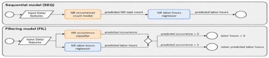
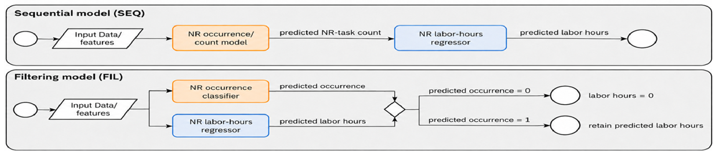
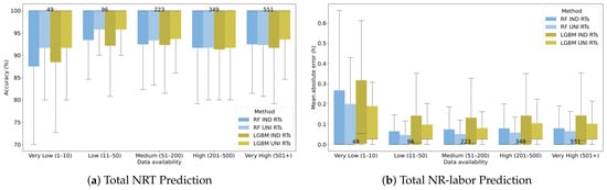
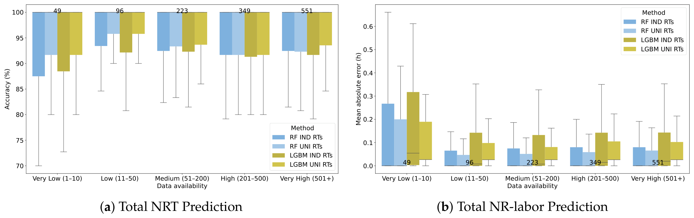
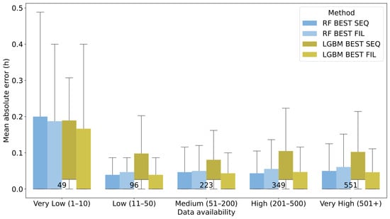
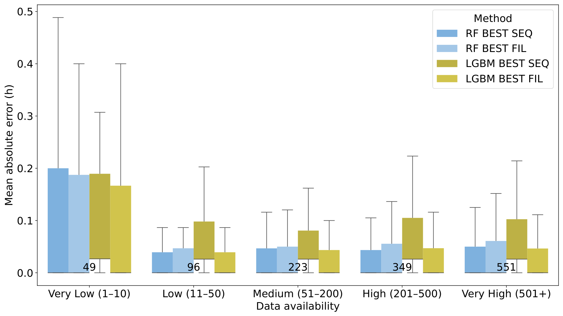
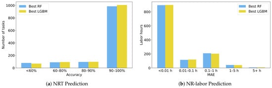
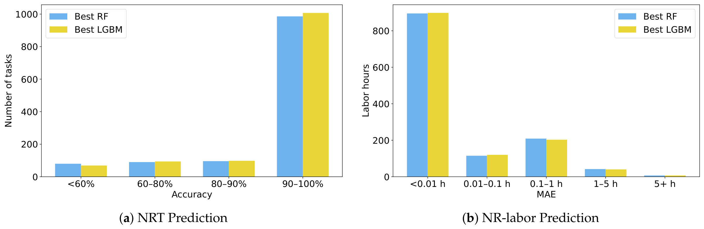
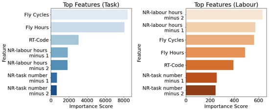
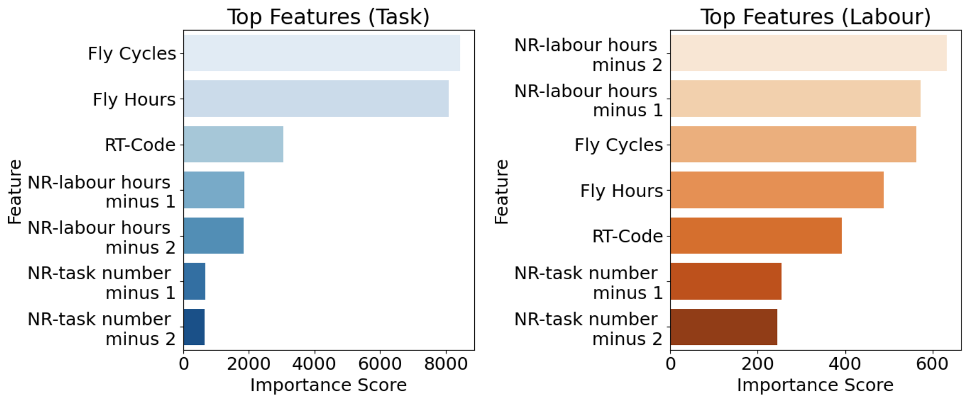
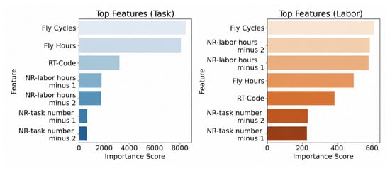
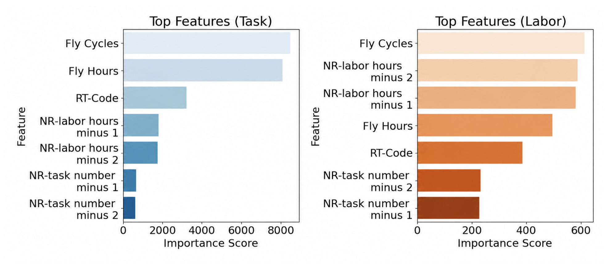
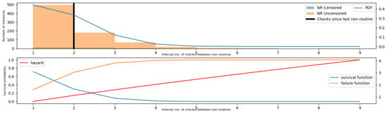
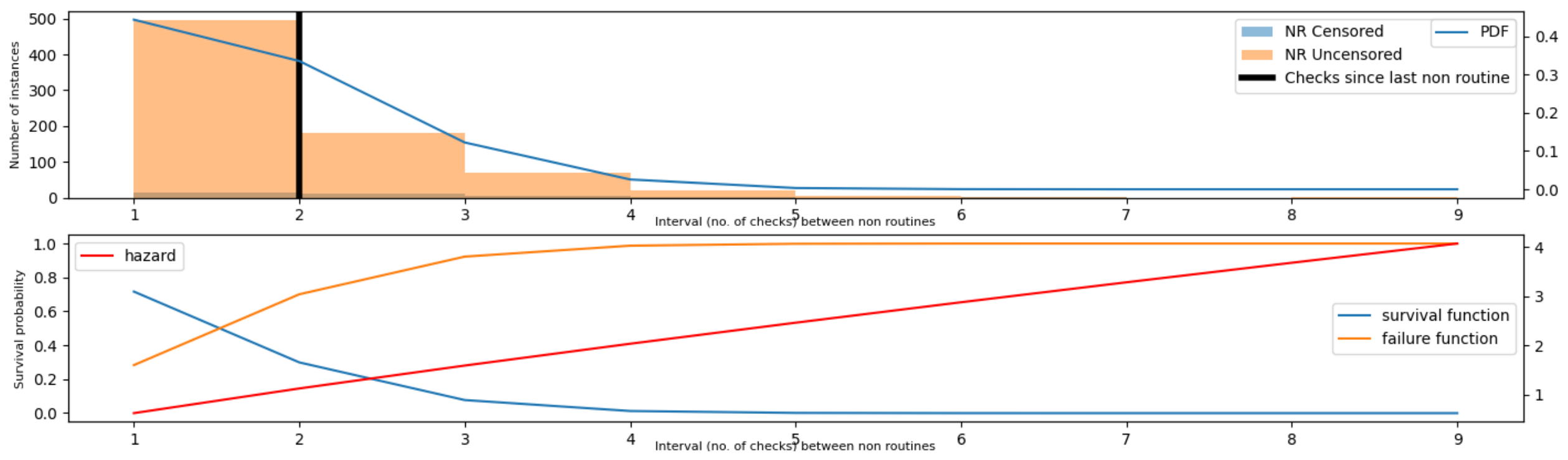
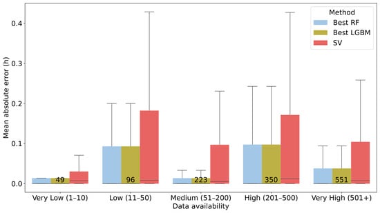
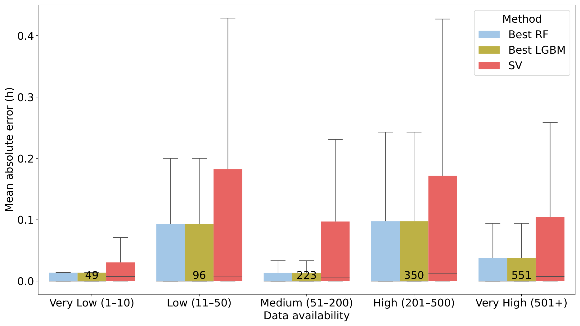
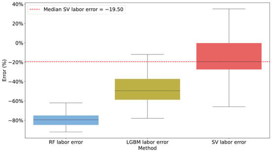
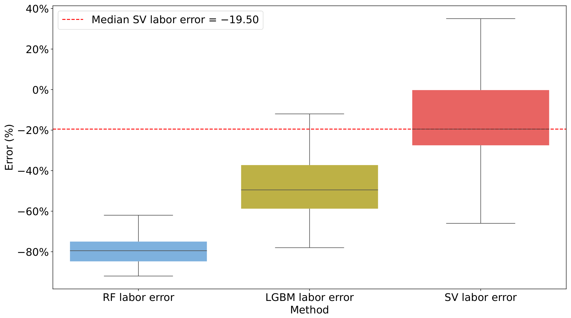
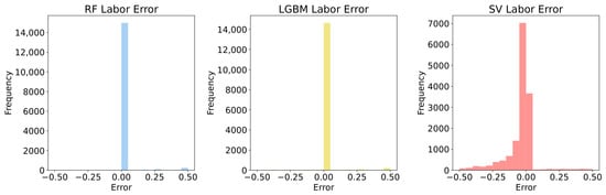
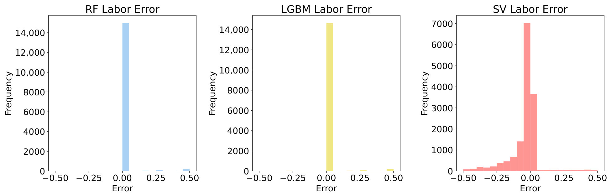

Disclaimer/Publisher’s Note: The statements, opinions and data contained in all publications are solely those of the individual author(s) and contributor(s) and not of MDPI and/or the editor(s). MDPI and/or the editor(s) disclaim responsibility for any injury to people or property resulting from any ideas, methods, instructions or products referred to in the content. |
© 2026 by the authors. Licensee MDPI, Basel, Switzerland. This article is an open access article distributed under the terms and conditions of the Creative Commons Attribution (CC BY) license.