


Abstract
Geospatial data provide an important basis for urban governance, resource management, disaster assessment, and public health analysis by linking spatial locations, attribute information, and dynamic processes. However, complex geospatial analysis still requires substantial expertise in spatial databases, spatial SQL, and GIS computation tools. Although large language model-based Text-to-SQL methods have lowered the barrier to natural language-driven data querying, most existing approaches rely on single-step SQL generation and remain unstable for spatial tasks that involve attribute retrieval, spatial relationship evaluation, geometric operations, and statistical aggregation. To address this limitation, this paper proposes a Code Generation-Driven Query–Computation Separation Framework (CGD-QCSF). The framework is based on the separation of query and computation, and decomposes complex geospatial analysis into a staged execution process. CGD-QCSF coordinates intent understanding, schema pre-filtering, planning, execution state management, SQL generation, and spatiotemporal computation. A structured planner and an execution state manager coordinate task decomposition, capability-aware routing, and evidence-based recovery. A SQL Code Generation Agent (SCGA) handles database access, attribute filtering, and intermediate data extraction, while a Spatiotemporal Computation Agent (STCA) performs out-of-database spatial computation and statistical aggregation in an isolated Python sandbox. We construct a benchmark of 200 tasks, covering easy, medium, and hard spatial tasks. In the main experiment with Qwen3.7-Plus as the foundation model, CGD-QCSF achieves a Strict Structured Accuracy (SSA) of 90.5%. Removing the Planner reduces SSA to 84.5%, while removing the STCA reduces it to 70.5%. The ablation experiments show that removing either the Python sandbox or the Planner Agent degrades performance on complex tasks. These results indicate that CGD-QCSF extends complex geospatial analysis from single-step SQL generation into a multi-staged execution process. By explicitly separating query and computation, the framework reduces interference between spatial computation logic and database schema information, thereby improving the stability and success rate of natural language-driven geospatial analysis.
1. Introduction
Geospatial data provide a fundamental basis for characterizing the real world and its dynamic changes. By linking spatial locations, attributes, and temporal processes, it supports the analysis of urban, resource, environmental, and social phenomena. Owing to this capability, geospatial data have been widely used in urban planning, resource management, disaster assessment, and public health, and have become an important support for scientific decision-making [1,2,3,4].
However, the effective use of geospatial data still involves a high technical barrier. On the one hand, modern geospatial data are increasing rapidly in scale, diversity, and complexity. Vector data, raster data, trajectories, remote sensing imagery, sensor observations, and thematic statistical data often coexist, exhibiting strong multimodal, heterogeneous, and cross-scale characteristics [5]. On the other hand, geospatial analysis typically depends on specialized data management systems and spatial computing tools. Non-expert users face significant barriers to performing such analyses directly, as they need to understand table structures, geometry fields, spatial indexes, and topological relationships in spatial databases such as PostGIS. They also need to master coordinate reference systems, spatial SQL syntax, and the underlying spatial computing toolchains [6,7]. These technical requirements make it difficult for non-specialists to directly use geospatial data and restrict many spatiotemporal analysis tasks to domain experts.
In recent years, large language models (LLMs) have made substantial progress in natural language understanding [8], code generation [9], and complex task solving. These advances enable broader access to geospatial analysis. In conventional relational database interaction scenarios, LLM-based Text-to-SQL methods have demonstrated practical usability [10]. These methods can convert natural language questions into structured SQL queries and can reliably support tasks such as attribute filtering, conditional querying, and general numerical aggregation. As a result, natural language-driven data querying has become an important direction for intelligent database interaction.
However, geospatial analysis differs substantially from conventional relational querying. Real-world geospatial analysis is not merely an SQL generation problem. It often involves operations on complex geometric objects and spatial topological relationships. It may also require coordinate transformation, distance measurement, buffer construction, spatial overlay, and regional statistics. Consequently, these tasks often involve strong inter-step dependencies and computational constraints. When existing Text-to-SQL methods or early single-step execution agents are directly applied to geospatial analysis, they still face two major challenges.
First, multi-step spatial reasoning often leads to instability in long-chain execution. Real-world spatial analysis tasks are rarely completed through a single SQL query or single-model generation. Instead, they usually involve multiple steps, such as data filtering, topological evaluation, spatial aggregation, and result sorting. These steps have clear input–output dependencies. An error in an earlier step may propagate to subsequent calculations [11]. Existing generative methods often lack explicit task planning and intermediate result verification mechanisms. Consequently, they are prone to field selection errors, spatial relationship misjudgments, and improper function calls during long-chain execution [12].
Second, large-scale spatial database schemas can easily cause context overload. Spatial databases usually contain numerous data tables, fields, geometry types, spatial indexes, metadata descriptions, and dedicated spatial functions. Feeding this information into the model without selection introduces substantial redundant context [13]. In long contexts, the model may overlook truly relevant tables, key fields, and geometric constraints. This can lead to incorrect table joins, invalid spatial function calls, or results that are inconsistent with the task semantics. It not only reduces the accuracy of query generation but also increases the risk of tool hallucination and syntax errors.
To address these challenges, this paper proposes a Code Generation-Driven Query–Computation Separation Framework (CGD-QCSF). The framework extends the reasoning and execution capabilities of conventional Text-to-SQL methods for complex geospatial analysis tasks. Rather than requiring a single generation step or a monolithic agent workflow to handle schema grounding, data retrieval, and spatial computation simultaneously, CGD-QCSF organizes these operations into role-specific execution stages. Code generation is used within two separate execution domains: the SCGA generates read-only SQL for database retrieval, whereas the STCA generates Python code for spatial and statistical computation. Planning and state management coordinate the execution of these two domains. This design improves the stability and auditability of complex spatiotemporal analysis tasks.
Specifically, CGD-QCSF contains intent understanding, schema pre-filtering, a Planner Agent, an Execution State Manager, an SQL Code Generation Agent (SCGA), and a Spatiotemporal Computation Agent (STCA). The framework first parses the user intent by identifying target objects, spatial scopes, attribute conditions, spatial constraints, and analysis goals. Then, the Planner Agent decomposes complex requirements into an executable sequence of subtasks. Based on the task type and intermediate results, the Execution State Manager dynamically schedules the SCGA and STCA. The Execution State Manager carries compact evidence between modules, enforces execution contracts, and applies bounded revise, repair, or replan transitions when a step fails. This forms a structured multi-step execution process involving planning, querying, computation, verification, and generation. The SCGA is primarily responsible for data querying within spatial databases. It transforms Text-to-SQL into a controllable data retrieval capability and combines it with intent parsing and schema pre-filtering mechanisms. These mechanisms identify task-relevant tables, fields, and constraint information from large-scale spatial database schemas. The agent mainly performs attribute filtering, spatial scope screening, basic table joins, and candidate feature retrieval. This reduces the interference of irrelevant schemas and redundant field information in the model context. In contrast, the STCA is responsible for complex spatial computation and result processing. It receives the data returned by the SCGA and generates Python code for subsequent operations, including buffer analysis, topological relationship evaluation, spatial clustering, and aggregation. In this way, the spatial database mainly handles data retrieval and basic filtering, whereas the Python environment is used for complex geometric logic and multi-step computation.
This design avoids forcing complex spatial logic into a single SQL query. It also reduces contextual interference caused by large-scale database schemas and decreases execution errors triggered by deeply nested spatial functions. Meanwhile, the Execution State Manager can inspect intermediate results during execution and adjust query conditions or computation paths when necessary. This capability improves the stability of long-chain spatial analysis tasks.
In summary, the main contributions of this study are as follows:
- We introduce CGD-QCSF, a Code Generation-Driven Query–Computation Separation Framework for complex geospatial analysis. It separates natural language tasks into controllable execution stages and coordinates planning, execution state management, SQL code generation, and spatiotemporal computation to improve execution stability.
- Within CGD-QCSF, we devise a decoupled query-and-computation mechanism to isolate SQL-based data retrieval from Python-powered spatial computation. This design mitigates schema-induced context overload and mitigates execution failures stemming from intricate nested spatial functions.
- We establish an evaluation protocol that considers both result correctness and process stability. Experiments on complex spatial analysis tasks and ablation variants show that CGD-QCSF improves final task completion, error recovery, and execution robustness.
2. Related Work
2.1. Text-to-SQL for Geospatial Queries
In recent years, large language models have made substantial progress in natural language understanding, code generation, and semantic reasoning. These advances have accelerated the development of Text-to-SQL technology [14]. Text-to-SQL aims to automatically convert natural language questions into executable SQL queries, thereby lowering the technical barrier for non-expert users to access and analyze structured databases. In general relational database scenarios, existing studies have extensively investigated key issues such as schema linking [15], semantic parsing [16], and query generation with execution feedback [17]. These methods can now reliably handle tasks such as attribute filtering, conditional querying, table joins, and general aggregation. They have also achieved strong performance on large-scale benchmarks such as Spider [18] and BIRD [19]. Relevant systematic evaluations further indicate that LLM-based Text-to-SQL methods have considerable potential for cross-database generalization and complex query generation [6,7,10].
As Text-to-SQL has matured, researchers have begun to extend it from conventional relational databases to spatial database scenarios. Typical target systems include relational databases with spatial extensions, such as PostgreSQL and PostGIS [20,21]. These databases are widely used in urban analysis [1], land-use planning [2], disaster monitoring [3], and public health [4]. Spatial queries differ from conventional relational queries in several important ways. They involve not only attribute fields and relational structures, but also geometric objects, spatial relationships, and spatial functions. Therefore, spatial semantics expressed in natural language must be mapped to database elements such as geometry columns, topological predicates, and spatial operators. For instance, expressions such as “intersects”, “contains”, “adjacent to”, and “within a certain range” usually need to be translated into specific spatial predicates or spatial function calls. Spatial Text-to-SQL is therefore not merely an SQL generation problem; it also requires spatial semantic parsing and the representation of spatial computation.
Existing work on spatial Text-to-SQL has mainly developed along three directions. The first direction concerns spatial semantic parsing, which seeks to map natural language constraints to executable spatial predicates in databases. To reduce the difficulty of mapping complex spatial operators, Kazazi et al. [22] proposed an AI-driven multi-agent framework to facilitate this translation. The second direction incorporates spatial knowledge enhancement to improve the model’s understanding of geographic entities and database structures. A typical approach is GeoRAG [23], which enhances question-answering models through geographic knowledge retrieval and helps LLMs perform geographic semantic reasoning. The third direction focuses on spatial function generation, guiding models to produce operations such as geometric construction, buffer analysis, and distance calculation. Within this scope, Li and Ning [24] developed an autonomous GIS agent (LLM-Geo) that leverages LLMs to generate Python code for complex spatial analysis, and Mansourian and Oucheikh [25] constructed ChatGeoAI, which translates natural language queries into PyQGIS scripts to execute spatial operations. Collectively, these studies suggest that rather than relying solely on conventional Text-to-SQL, integrating it with spatial code generation holds the potential to support a broader range of complex GIS-oriented tasks.
2.2. LLM Agents for Geospatial Analysis
To overcome the limitations of single-step Text-to-SQL methods in handling complex tasks, researchers have increasingly introduced agent-based approaches built on large language models. Agents typically address complex tasks through task planning, tool use, code execution, and result feedback [8]. Representative studies include ReAct [26] and Toolformer [27]. Compared with methods that generate SQL in a single step, agents can decompose complex problems into multiple executable steps and adjust subsequent actions based on intermediate results. This multi-step reasoning and feedback mechanism offers a promising direction for complex geospatial analysis.
Early studies mostly adopted a single-agent framework, where one agent integrates multiple functions such as requirement understanding, code generation, tool invocation, and result interpretation [24,25]. This design is structurally simple and well suited for spatial tasks with short workflows and a limited number of tools. By invoking database interfaces or Python libraries, these agents can effectively handle data retrieval, geometric processing, and statistical computation. A representative work in this paradigm is GIS Copilot, proposed by Akinboyewa et al. [28], which functions as an autonomous agent that generates Python code and calls specialized tools for geospatial task execution. Collectively, these studies demonstrate that coupling LLMs with external spatial computation utilities can, to a certain extent, improve the automation of geospatial analysis.
However, single-agent frameworks become less reliable when applied to complex geospatial workflows. In such settings, the agent is expected to interpret the task, identify relevant data, generate executable queries or code, invoke appropriate tools, and assess the returned results within the same reasoning process. This broad scope of responsibility increases the likelihood of unstable execution, especially because geospatial tasks often combine attribute filtering, topological reasoning, geometric computation, and result presentation. These operations rely on different data representations and computational tools, making it difficult for a single agent to maintain a consistent execution path. Consequently, complex tool environments may lead to incorrect tool selection, fragmented reasoning, and excessive context load [29,30].
To alleviate the capability bottleneck of single agents in complex tasks, recent studies have increasingly adopted role-based agent workflows. In these workflows, planning, code generation, tool execution, and result checking are assigned to different roles: a task planner is responsible for problem decomposition; a code generator is responsible for generating SQL or Python code; an executor is responsible for calling tools; a reviewer is responsible for checking result consistency [31,32]. For example, Luo et al. proposed the GeoJSON Agents framework. Through multi-agent collaboration, it achieves switching between tool calling and code generation in geospatial analysis [31]. Yang et al. utilized a multi-agent system to build a geospatial knowledge base question-answering system. This improved the answering accuracy for complex geographic questions [32]. This role separation narrows the responsibility of each execution stage and makes dependencies between planning, retrieval, computation, and review more explicit. In the field of geospatial analysis, multi-agent methods have been used for tasks such as data discovery, spatial querying, code execution, result checking, and map production [33,34,35]. These studies indicate that phased reasoning and tool synergy can further expand the application capabilities of large language models in GIS scenarios [36].
Despite these advances, existing agent-based methods still face an important challenge. A common way to extend agent capability is to register additional tools [37]. These tools include database-native spatial functions as well as external Python libraries such as GeoPandas, Shapely, and PySAL [38]. A rich toolset can increase task coverage, but it also makes tool selection more difficult for the model. When database schemas, spatial function descriptions, and external library documentation are exposed to the model at the same time, the system is more likely to encounter context overload, tool selection errors, and unstable computation paths [30]. This problem is especially common for spatial operations with similar functions.
Existing approaches also differ in their task objectives and execution boundaries. Spatial Text-to-SQL methods primarily generate spatial SQL for operations computable within databases, whereas retrieval-augmented approaches such as GeoRAG [23] focus on geographic question answering. ChatGeoAI [25] translates natural language requests into scripts executed in a QGIS or PyQGIS environment, while GIS Copilot [28] and LLM-Geo [24] mainly generate Python-based geospatial workflows.
Different from these paradigms, CGD-QCSF targets question answering over structured spatial databases and defines an execution contract that integrates task-specific schema grounding, read-only SQL retrieval, JSON or GeoJSON intermediate-data export, restricted Python computation, and structured evidence review. This contract logically decouples database retrieval from geometric, statistical, and machine learning computation, while maintaining explicit dependencies between these two computation stages.
3. Methodology
3.1. Overall Framework
This section presents the overall framework and data flow of CGD-QCSF. Given a natural language spatial query and a global spatial database schema , CGD-QCSF defines a mapping process . Here, denotes the set of executed actions, which are explicitly divided into database-oriented query actions and Python-oriented computation actions . denotes the generated intermediate data files. During iterative execution, the system continuously tracks and updates its execution state . Section 3.2, Section 3.3, Section 3.4, Section 3.5 and Section 3.6 describe the methodological design of each module in detail.
The core design of CGD-QCSF is query–computation separation. Existing approaches may require a single SQL statement or a monolithic agent invocation to handle schema grounding, relational retrieval, geometric processing, and statistical analysis within the same execution context, which increases generation difficulty and intensifies the interference between schema information and spatial computation logic. To address this issue, CGD-QCSF divides system actions into two types. The first type is the query action , which generates SQL and retrieves data from the spatial database. The second type is the computation action , which generates Python code and performs spatiotemporal analysis in an isolated execution environment.
Under this design, the database is mainly responsible for structured retrieval, attribute filtering, joins, and preliminary aggregation. The Python environment handles geometric operations, spatial topology evaluation, statistical analysis, and other high-level computations. The two domains are connected through typed JSON or GeoJSON artifacts. Their field names, file formats, and geometry types constitute an explicit interface contract between database retrieval and downstream computation. This contract preserves the data dependencies of multi-stage tasks while separating the responsibilities, execution constraints, and validation rules of SQL generation and Python computation.
From the workflow perspective, CGD-QCSF can be represented as an iterative reasoning and execution process over a directed state graph, as shown in Figure 1. Given the query , the system first performs intent understanding and schema pre-filtering to obtain a local schema subset relevant to the task. The Planner Agent then generates an ordered subtask sequence and structured execution constraints. In the following iterations, the Execution State Manager invokes either the SCGA or the STCA according to the current step’s declared capability, input dependencies, and success criteria. After each execution step, the Execution State Manager updates its execution state based on the returned result and determines whether to continue, revise the current step, repair an upstream dependency, replan, or terminate. Simple relational tasks may terminate after the SCGA produces sufficient evidence, whereas tasks involving geometry, statistics, or machine learning continue through an SQL-to-Python path. The SCGA exports intermediate query results as JSON or GeoJSON files, and the execution state stores only their references and compact previews. When Python computation is required, the STCA consumes these files rather than receiving the complete result sets through the model context.
Figure 1.
Directed state graph of CGD-QCSF.
3.2. Intent Understanding with Schema Pre-Filtering
The complete database schema is typically large in scale. Feeding the entire global schema directly into the model raises context overhead and incorporates plenty of irrelevant content for the target task. To reduce this burden, CGD-QCSF adopts intent understanding with schema pre-filtering. This process constructs a query-specific local schema subset from the global schema . It can be represented as the mapping .
First, the system parses the natural language spatial query into an intent tuple . This tuple describes the query intent from five dimensions. Their definitions are provided in Table 1.
Table 1.
Definitions of five dimensions in Intent Tuple .
Here, represents the analysis objects and metric contents. represents the analysis operation type. They correspond to what should be analyzed and how the analysis should be performed, respectively. For the spatiotemporal scope , the system further performs geographic hierarchy completion to reduce matching ambiguity caused by multi-scale spatial references. For instance, a user may refer to “Wuhan City”, whereas the database may only contain provincial-level tables. In this case, the geographic hierarchy inference function maps the entity to its higher-level administrative unit, thereby increasing the likelihood of successful table retrieval. If the input is not related to a geospatial analysis task, the execution control dimension marks it as a rejection type and terminates the subsequent workflow.
After obtaining the structured intent tuple , the system enters the relevant schema retrieval stage. Real-world spatial databases typically exhibit high schema heterogeneity, encompassing massive interconnected tables, complex geometric representations, and diverse spatiotemporal attributes. Directly providing the full global schema via the raw Data Definition Language (DDL) can introduce errors, such as incorrect joins, missing fields, or absent spatiotemporal filtering conditions. To bridge the semantic gap between natural language queries and the underlying database, the system organizes semantically enriched schema information for each candidate table. This information is represented as , where the four components correspond to thematic content, spatiotemporal attributes, field semantics, and table relationship information, respectively.
First, the system leverages the thematic content and field semantics to perform hierarchical vector retrieval. At the table level, summaries integrate the business meaning and associated geographic regions to establish the target domain. At the column level, summaries capture field descriptions, enumerated values, and explanations of common abbreviations to identify specific metrics and their semantics. During scoring, the column-level similarity is weighted more heavily (), and the final score combines table-level and column-level similarities. This weighting strategy prioritizes the retrieval of tables containing the user’s target metrics.
The spatiotemporal attributes serve as hard filtering conditions by specifying the temporal and spatial resolutions of the data, such as annual, monthly, state-level, or grid-level granularity. For example, when a query requests fine-grained data for “March 2020,” the system excludes tables containing only annual data. Similarly, if a query requires state-level aggregation, grid-level tables unsuitable for direct aggregation are removed. These constraints reduce the risk of spatiotemporal granularity mismatches during subsequent code generation.
After selecting the core candidate tables, the system uses the table relationship information to complete the associated tables required for execution. records primary–foreign key relationships, spatial feature codes, and join rules between attribute tables and boundary tables. Based on this information, the system automatically introduces the necessary geometry tables and removes unmatched irrelevant columns. After this filtering and completion process, the system obtains the local schema subset . This subset provides the subsequent SCGA with a concise and well-structured schema context, thereby reducing contextual interference caused by large-scale schema structures.
3.3. Planner Agent: Task Decomposition and Execution Constraint Generation
Complex spatiotemporal queries often involve data retrieval, spatial reasoning, and statistical computation within the same task. Forcing these processes into a single generation step requires the model to handle multiple objectives at once, which increases the likelihood of generation errors. To address this issue, CGD-QCSF introduces a Planner Agent. The Planner Agent receives the structured intent tuple and the local schema subset , and generates the subtask sequence and the structured execution constraints . This process can be denoted as .
In the subtask sequence , each subtask corresponds to either an SQL generation call or a Python code generation call. Each step is stored as a structured object containing the selected tool, objective, input dependencies, and success criteria. The system generates an initial sequence based on and , while restricting each step to one of two categories: SQL retrieval or Python-based spatiotemporal computation. This constraint preserves the separation between query and computation. The sequence length is determined by the required execution capabilities and data dependencies rather than by the benchmark difficulty label. For simple queries involving aggregation, sorting, or attribute filtering, a single SQL retrieval step is usually sufficient. For tasks involving spatial topological relations or spatial statistics, the system generally adopts a two-step structure in which data are retrieved first and then processed in the Python environment.
After generating the initial subtask sequence, the system applies step consolidation to reduce excessive decomposition. The consolidation criteria differ for SQL retrieval and Python computation, requiring separate handling. On the SQL retrieval side, multiple extractions within the same data preparation round are merged into a single SCGA call. This reduces redundant schema retrieval, prompt construction, database access, result exporting, and task scheduling overhead. Within each call, the system can still generate multiple SQL statements and export multiple result files to accommodate multi-table extraction.
On the Python computation side, the sandbox does not retain interpreter variables or in-memory intermediate results across adjacent calls. Splitting a continuous analysis chain into multiple calls typically requires bridging them via temporary files, increasing I/O overhead and the risk of failure. Therefore, if multiple computations target the same analysis and can be executed sequentially within a single script, they are consolidated into one Python call. When subsequent computations do not rely on geometric information, the SQL stage exports only JSON attribute data, reducing unnecessary geometric processing.
In addition to generating the subtask sequence, the Planner Agent produces the structured execution constraints . These constraints are generated from the intent tuple and the subtask sequence , and explicitly define the requirements that subsequent code generation must satisfy. The field definitions are summarized in Table 2. By providing unified constraints for both SQL and Python code generation, reduces ambiguity during execution and improves consistency across different workflow steps.
Table 2.
Definitions of constraint fields in Structured Execution Constraints .
3.4. Execution State Manager, Evidence Review, and Final Answer Contract
The Execution State Manager contains only the information required for subsequent execution decisions. An associated execution log separately records end-to-end time, Prompt, Completion, and Total Tokens, tool-trace steps, failed calls, and framework-level recovery transitions. Large database results are not copied into the state. Instead, the state retains file references, compact previews, and the evidence required to determine whether the current step has been completed.
The SCGA and STCA do not modify the global plan directly. Instead, they return structured results containing status, evidence, and error type, from which the state manager selects a continue, revise, repair, replan, or terminate transition. All local retries, recovery transitions, and graph traversal are bounded by configurable limits.
After a candidate answer is generated, an independent evidence-review node reads only the question, answer contract, executed-tool evidence, and a compact state summary, and returns accept, revise, repair, or replan. The workflow terminates when the available evidence supports the candidate answer. An accept decision is converted by the state manager into a terminate transition. A revise decision corrects fields, ordering, units, or answer projection when they conflict with the available evidence. A repair decision returns to the relevant upstream step when required evidence is absent, whereas a replan decision is used when the existing execution blueprint cannot produce the required answer.
The final answer is emitted as a constrained object containing explicit answer_type and data_payload fields. This protocol supports scalar answers, entity lists, ranked records, record collections, and nested spatial objects. Conformance to this protocol is evaluated separately from semantic correctness: schema validity checks whether the returned object satisfies the declared output structure, while Strict Structured Accuracy evaluates whether its structured content matches the verified task result. Figure 2 summarizes the evidence-review decisions and bounded-recovery transitions.
Figure 2.
Evidence review, state transition, and bounded recovery. Solid black arrows indicate the main state-transition flow; the green arrow indicates acceptance, while the colored dashed arrows indicate feedback paths for the corresponding recovery actions.
3.5. SQL Code Generation Agent: Data Retrieval and File Export
CGD-QCSF encapsulates SQL generation as an independent module to ensure that data retrieval remains verifiable and auditable. The SCGA is responsible for executing the query subtask . Given the current subtask, the SCGA generates one or more executable SQL statements, runs them in the database, and exports the returned results as structured files. These files either provide evidence for final answer generation or serve as input to the STCA when downstream computation is required.
Before SQL generation, the system further filters relevant tables from the local schema subset according to the current subtask. This step differs from the schema retrieval process in Section 3.2. The earlier retrieval uses the original user query as input, whereas the current retrieval uses the subtask description produced by the Planner Agent. As a result, the retrieved schema information is more closely aligned with the current execution step. For repeated attempts of the same subtask, the system reuses cached retrieval results. The input to the SQL generation model includes the active subtask, the original user query, and the filtered table schema. The original query is retained to preserve details such as spatiotemporal scopes, metric names, and constraint conditions, thereby reducing information loss caused by task decomposition. When applicable, the input also includes execution constraints and requirements derived from the answer contract, such as whether the result must be ordered, bounded, or exported with geometry.
To ensure safety and consistency during execution, each SQL statement is validated against a set of static rules before being submitted to the database engine. The validation rules are listed in Table 3.
Table 3.
SQL validation rules of SCGA.
In addition to static validation, the system employs an error correction mechanism based on execution feedback. If an SQL statement passes validation but fails to execute on the database, the executor records the returned error information, which may include syntax errors, missing columns, type mismatches, or grouping conflicts. The system then uses the current subtask, the previous SQL, relevant schema fragments, and the error log as feedback to guide the next SQL generation attempt. This local correction remains within the active query step. If the retry budget is exhausted or the failure indicates an incorrect upstream plan or missing dependency, the SCGA returns structured failure evidence to the Execution State Manager rather than modifying the global plan directly.
After successful execution, the query results are written to the working directory as files, denoted as . Data containing geometries are exported in GeoJSON format, whereas purely attribute data are exported as JSON. According to the state representation described in Section 3.1, the execution state records only the file path reference and a brief result preview, rather than the complete result set. This design keeps large result sets outside the model context. For SQL-only tasks, the exported evidence can be used directly for answer generation and review; when further computation is required, the STCA reads the referenced files. The SCGA therefore supports execution-guided correction rather than assuming that every query will succeed in a single generation attempt.
3.6. Spatiotemporal Computation Agent: Python Code Generation and Spatial Computation
To decouple high-level spatial analysis from database retrieval, CGD-QCSF introduces the STCA, which is responsible for executing the computation subtask . The STCA reads the data files exported from the SQL stage, generates Python analysis scripts, and executes them within a restricted sandbox environment supported by unified output protocols and adaptive error correction mechanisms.
Because the STCA cannot directly access the database, code generation relies on file paths, the local schema subset, and execution constraints to infer the required analysis logic. Accordingly, the system provides the agent with the current subtask, execution constraints, the list of input files, the upstream SQL statements, and the user’s intent. The structure of this input context is summarized in Table 4.
Table 4.
Code generation input context for STCA.
The aforementioned information collectively forms the conditional input for code generation. Let denote the Python script generated by the STCA. Here, specifies explicit constraints on the geometry requirement, input mode, and operation category, thereby narrowing the space of feasible code.
To enable consistent parsing of execution results, the generated scripts must follow a unified output protocol. After execution, each script writes the final JSON object to the standard output. The top-level object must contain exactly three keys: status, summary, and result. The value of status is either success or error. The summary field provides a natural language response for the user, whereas result stores numerical or tabular structured results as either an object or an array. An example is shown below:
| { “status”: “success”, “summary”: “The Spearman correlation coefficient between annual average precipitation and NDVI across counties in California from 2015 to 2020 was 0.42.”, “result”: {“metric”: “spearman_r”, “value”: 0.42, “n”: 58} } |
Based on this protocol, the system can read the script outputs without parsing the internal control flow of the scripts. This allows the Planner Agent to consume structured results and advance to subsequent subtasks or final answer synthesis without reinterpreting Python execution logic. Because the scripts are automatically generated, they are executed within an isolated sandbox to mitigate security risks. The sandbox environment is pre-installed with standard libraries such as GeoPandas, Shapely, Pandas, and NumPy, with software versions fixed to ensure consistent experimental conditions. Each script runs in an independent process and can only access files exported from the upstream SQL stage and a limited set of runtime metadata. It cannot access database connections, external networks, sensitive host directories, or create new processes. Additionally, the system enforces restrictions on memory usage, CPU time, and the writable scope of temporary directories to control execution risks.
For execution control, the system employs two error correction mechanisms. The first is the code-level adaptive retry. When a Python script encounters a runtime exception in the sandbox, the executor records the standard error stream (stderr). Common exceptions include IndexError, ValueError, and analysis failures due to invalid geometry. The system then constructs feedback information using the failed script, input file summaries, upstream SQL, the current subtask, and the stderr log to guide the next round of code generation. The stderr provides the exception type, error location, and stack trace, enabling subsequent corrections to focus specifically on the identified error. The second mechanism is global dependency backtracking. When an exception satisfies two conditions, the system classifies it as a missing data dependency rather than a code logic error. First, the exception type must belong to a predefined whitelist of dependency-related errors, such as KeyError, missing fields, or field parsing failures. Second, the error identifier must be matched against upstream SQL result columns, JSON keys, or the field set of a GeoDataFrame. If both conditions are met, the failure is likely caused by unexported upstream data, inconsistent field naming, or omissions in the Planner Agent. The system then suspends the current computation step and returns structured anomaly feedback to the Planner Agent, which triggers SQL regeneration and supplementary data extraction. If the problem originates from missing dependencies in the planning stage, the system updates the subtask constraints. If the planning is correct but the SQL output lacks required fields, the system regenerates the SQL and exports supplementary data. Once the new becomes available, the system resumes the current computation step.
Through these two mechanisms, the system distinguishes code implementation errors from data dependency errors. The former are corrected through local retries, whereas the latter are handled through cross-step backtracking. This design allows spatiotemporal computation to remain recoverable under runtime exceptions, geometry validity errors, and missing fields. The effectiveness of these error correction mechanisms is quantitatively evaluated in the ablation study in Section 4.
4. Experiments
4.1. Benchmark and Experimental Setup
To evaluate the effectiveness of CGD-QCSF, we constructed a benchmark for spatial querying and spatial computation tasks. All experiments were conducted in a unified environment. The experiments comprise a foundation model comparison, controlled architecture baselines, internal ablations, and an adapted external baseline. All configurations are evaluated on the same 200-question benchmark and database snapshot.
The benchmark contains 200 spatial tasks. All samples were manually designed and verified. Each sample includes a natural language question, a difficulty label, an execution module requirement annotation, reference SQL logic, reference Python code, and the expected execution result, as shown in Table 5. The reference Python code is provided only for tasks that require out-of-database spatial computation or statistical processing. The expected execution result serves as the basis for end-to-end evaluation and error analysis.
Table 5.
Structure of each benchmark sample.
The benchmark covers two typical data scenarios: U.S. state-level spatial data and Zhejiang Province 1 km × 1 km vector fishnet cells. Tasks are divided into three categories based on execution complexity, easy, medium, and hard, as shown in Figure 3. The dataset contains 66 easy questions, 64 medium questions, and 70 hard questions. The easy questions generally involve single-table filtering, counting, sorting, or Top-K selection. The medium questions generally require joins, grouped aggregation, period comparison, or computation relative to a global baseline. The hard questions generally involve geometric topology, distance or buffer operations, multiple intermediate files, regression, clustering, hypothesis testing, or multi-stage composite computation. By primary analytical objective, the 200 questions comprise 54 attribute retrieval, conditional filtering, or ranking tasks; 61 grouped aggregation or composite indicator tasks; 21 temporal comparison or change analysis tasks; 19 spatial geometry, topology, or distance tasks; and 45 statistical, machine learning, or uncertainty analysis tasks. According to the verified execution path, 134 questions can be completed through the SQL channel, whereas 66 require SQL retrieval followed by Python sandbox computation.
Figure 3.
Distribution of benchmark task difficulty and sandbox requirement ().
The experiments include three sets of configurations. The first set is the model capability experiment. It uses Qwen3.7-Max (qwen3.7-max-2026-05-17), Qwen3.7-Plus (qwen3.7-plus-2026-05-26), and Qwen3.6-Flash (qwen3.6-flash-2026-04-16), provided by Alibaba Cloud (Hangzhou, China), as well as DeepSeek-V4-Flash and DeepSeek-V4-Pro, developed by DeepSeek (Hangzhou, China), as foundation models. All model configurations use identical framework prompts, the same benchmark and database snapshot, and a temperature of 0. This compares the differences among models in spatial task understanding, planning reasoning, and code generation. The second set is the architecture study, which includes two controlled baselines, Standard ReAct and Standard Plan-and-Execute, and one adapted external baseline, LLM-Geo. The third set is the architecture ablation experiment. It compares five system configurations under a fixed foundation model setup: FULL (Ours), +PostGIS, w/o STCA, w/o Planner, and Base. FULL represents the complete CGD-QCSF framework. In this configuration, the SCGA is only responsible for relational queries and basic data retrieval. It is not allowed to directly call PostGIS spatial functions in SQL. +PostGIS enables SQL-side spatial function calls based on the complete framework. The w/o STCA configuration removes the STCA and the Python sandbox. The w/o Planner configuration removes the Planner Agent. The Base configuration only retains standard relational SQL query capabilities. Through these configurations, we can respectively analyze the impacts of spatial function, external computation sandboxes, and planning mechanisms on system performance.
All experiments record complete execution logs. These logs include subtask routing paths, SQL query results, Python sandbox outputs, final answers, failed tool calls, guardrail retry counts, and Token consumption. These logs are used for subsequent performance comparison, ablation analysis, and error attribution. The evaluator compares the structured payload of the final answer with the verified expected result. It does not require generated SQL or Python code to match the reference source code, but it does not use a free-text coverage fallback when the structured payload is incorrect.
The experiments were conducted on a local workstation equipped with 20 logical cores and 40 GB of memory. The underlying data service uses PostgreSQL 16.7 and the PostGIS extension. To avoid resource exhaustion caused by unbounded spatial queries, the SQL execution layer sets a 30 s timeout threshold and a maximum return limit of 100,000 rows. The code generated by the STCA runs in an isolated Python 3.12 subprocess sandbox. The sandbox is pre-installed with core spatial computation libraries such as GeoPandas and Shapely.
The experiments access large language models through APIs and do not load model weights on the local machine. Local memory is used primarily for Agent state, schema indexes, database results, intermediate files, and the Python sandbox, whose configured limit is 2 GB. Because peak resident set size was not continuously collected for every process, the resource analysis does not report peak-memory measurements.
To control context expansion caused by large-scale spatial metadata, the system applies unified constraints to context inputs. Historical dialogs only retain the most recent 10 turns. Schema Pre-filtering introduces a maximum of eight highly relevant data tables each time. The foreign key expansion depth between tables does not exceed three levels. These settings are used to constrain the context size while simulating system operation scenarios under limited resource conditions in real-world deployments.
4.2. Evaluation Framework and Metrics
We evaluate system performance from four aspects: result correctness, task routing, execution efficiency, and system stability. First, Strict Structured Accuracy (SSA) is used to measure the consistency between the system’s final output and the expected result. For the -th sample, only when the execution succeeds, the returned object conforms to the final answer contract, and its structured data_payload matches the manually verified ground truth under the evaluation rules described below. Otherwise, it is recorded as . SSA is defined as follows:
SSA is evaluated on the final structured output rather than on free-text answer coverage. Scalar answers must appear in an explicit answer field or a single-valued payload. When an entity and an associated value are required, they must occur within the same record. Ordinary lists permit neither missing nor additional records, whereas ranked lists are compared in order.
Numeric comparison first verifies field semantics and then applies predefined unit normalization, ratio conversion, and numerical tolerances. Distances are converted to meters, integer identifiers are compared exactly, and flat and nested BoundingBox representations are treated as equivalent when their four boundary values agree. Dictionary outputs may contain additional explanatory fields that do not alter the answer semantics, but every field required by the verified answer must be correct. Generated SQL and Python code are not required to be textually identical to the reference implementations; correctness is determined from the resulting structured answer.
For questions whose expected answers are entity lists or record lists, the evaluator additionally reports Exact Set Match, Ranking Exact Match, and entity-level Precision, Recall, and . Let and denote the predicted and verified entity sets for an eligible list question. Entity-level Precision, Recall and are defined as follows:
Exact Set Match equals 1 when the predicted and verified entity sets are identical. Ranking Exact Match additionally requires the returned sequence to match the verified order. These list-specific metrics are undefined for scalar and dictionary questions and are excluded from the corresponding aggregate denominator.
Next, the routing quality is evaluated. The system treats whether a Python sandbox is required as a binary ground-truth label. The predicted label is obtained from the actual execution trace, depending on whether the Python sandbox is invoked. This yields the confusion matrix counts , , , and . The full-sample Routing Accuracy (RA) is defined as follows:
It also reports Precision P = TP/(TP + FP), Recall R = TP/(TP + FN), and their harmonic mean:
In addition, we report the false positive routing rate for sandbox routing, defined as FP/(FP + TN). This characterizes the proportion of tasks not requiring a sandbox that are incorrectly routed to the sandbox.
Execution efficiency is characterized by end-to-end time and Token consumption. Let and denote the end-to-end execution time and total number of Prompt and Completion Tokens for the -th question. Their mean values are as follows:
End-to-end time includes planning, model invocation, database execution, Python computation where applicable, evidence review, and final answer generation. Token statistics are also retained separately as Prompt, Completion, and Total Tokens in the execution logs.
The First Execution Path Success Rate (FEPSR) is used to distinguish final task success from success achieved without a failed tool call or framework-level recovery transition. Let denote the number of failed tool calls and the number of guardrail retries for the -th question. A failed call is a tool-trace entry whose status is failed. A guardrail retry is an explicit framework-level correction transition and is distinct from an ordinary successful progression between workflow steps.
FEPSR is then
SSA remains the primary correctness metric because a correct answer obtained after bounded recovery still represents successful task completion. FEPSR instead measures the proportion of questions that are answered correctly along the first execution path without failed calls or framework-level recovery.
4.3. Foundation Model Comparison
This section compares the overall performance of different foundation models under the complete CGD-QCSF architecture. The comparison focuses on two aspects: final result correctness and execution overhead and stability. Table 6 reports the overall results.
Table 6.
Overall performance of different base models under FULL configuration.
Regarding final result correctness, Qwen3.7-Max achieves the highest Strict Structured Accuracy at 96.0%. It exceeds DeepSeek-V4-Pro, the second-best model, by 4.0 percentage points. DeepSeek-V4-Pro reaches 92.0%, while Qwen3.7-Plus and DeepSeek-V4-Flash both obtain 90.5%. Qwen3.6-Flash records the lowest SSA at 85.5%. These results suggest that stronger foundation models tend to produce higher SSA under the same system architecture. In particular, stronger model capability helps the system complete spatial queries, spatial relationship evaluation, and multi-step spatial computation tasks more reliably.
Tasks of varying difficulties further amplify the differences among models, as shown in Figure 4. On easy tasks, the SSA of all five models approaches or reaches . This indicates that easy tasks primarily rely on table field recognition and basic SQL generation capabilities. Their requirements for model reasoning capabilities are relatively limited. However, the performance gap among models widens significantly on medium and hard tasks. The SSA of Qwen3.7-Max on hard tasks is . In contrast, Qwen3.7-Plus and Qwen3.6-Flash achieve and , respectively. This demonstrates that factors such as aggregation queries, cross-table joins, spatial relationship recognition, multi-step execution, and out-of-database computation significantly increase task complexity. These factors further amplify the capability differences among foundation models.
Figure 4.
Strict structured accuracy by task difficulty for different foundation models under the FULL configuration.
Routing Accuracy ranges from 89.5% to 93.5%. Qwen3.7-Max and Qwen3.6-Flash both achieve the highest Routing Accuracy of 93.5%, followed by Qwen3.7-Plus at 91.5%, DeepSeek-V4-Flash at 90.5%, and DeepSeek-V4-Pro at 89.5%. The result shows that routing accuracy is related to, but not determined by, overall answer correctness. In particular, Qwen3.6-Flash matches Qwen3.7-Max in routing accuracy despite having an SSA that is 10.5 percentage points lower. Correct execution channel selection is therefore necessary but insufficient for final task success. Errors may still arise during schema grounding, SQL generation, Python computation, evidence projection, or structured answer generation. These results demonstrate that foundation model differences not only affect final answer correctness. They also affect the reliability of module routing and the stability of computation paths.
The FEPSR provides a stricter view of execution stability by requiring a correct final answer without failed tool calls or framework-level recovery transitions. Qwen3.7-Max achieves the highest FEPSR at 92.0%, only 4.0 percentage points below its SSA. The corresponding SSA–FEPSR gaps are 5.5 points for Qwen3.7-Plus, 4.5 points for Qwen3.6-Flash, 8.0 points for DeepSeek-V4-Flash, and 13.0 points for DeepSeek-V4-Pro. The comparison demonstrates that final correctness and execution stability should be analyzed separately rather than treated as interchangeable measures.
Overall, Qwen3.7-Max provides the best combined performance across SSA, Entity , FEPSR, Routing Accuracy, execution time, and Token consumption. DeepSeek-V4-Pro ranks second in final SSA but depends more heavily on recovery, as reflected by its lower FEPSR and larger SSA–FEPSR gap. DeepSeek-V4-Flash produces fewer fully correct answers than the Pro configuration but achieves higher first-path stability, slightly stronger entity matching, and lower execution time. Qwen3.7-Plus provides a balanced intermediate result and is retained as the fixed foundation model for the subsequent architecture baseline and ablation experiments.
4.4. Architecture Baselines Comparison
This section compares the complete CGD-QCSF architecture with two controlled agent baselines and one adapted external baseline. All experiments in this section use Qwen3.7-Plus as the foundation model. FULL, Standard ReAct, and Standard Plan-and-Execute use the same 200-question benchmark, database snapshot, schema-retrieval procedure, SCGA and STCA, structured output protocol, and basic safety and error-handling settings. Their main difference lies in the workflow control policy. Standard ReAct follows a Thought–Action–Observation loop. It selects and invokes a tool according to the current question and accumulated observations, and then uses the returned evidence to determine the next action. In contrast, Standard Plan-and-Execute separates planning from execution. It first generates a complete sequence of actions and then executes the resulting plan. The initial plan remains fixed during execution.
LLM-Geo is included as an adapted external baseline. Its original design is oriented toward generating and executing geospatial Python workflows. To evaluate it on the database-grounded benchmark used in this study, its inputs and outputs are adapted to the benchmark questions, available geospatial data, and structured evaluation protocol. The experimental results are reported in Figure 5, and the comparison of overall answer coverage is shown in Table 7.
Figure 5.
Architecture baseline comparison in strict structured accuracy, entity matching, and routing.
Table 7.
Comparison with controlled architecture baselines and adapted external baseline using Qwen3.7-Plus ().
Among the controlled configurations, Standard ReAct achieves the closest result to FULL. Its SSA reaches 87.5%, which is 3.0 percentage points lower than that of FULL. The difference increases on hard questions: FULL obtains 85.7%, whereas ReAct reaches 77.1%, producing a gap of 8.6 percentage points. This larger difference on hard tasks suggests that incremental action selection remains effective for many ordinary queries but is less reliable when execution depends on multi-stage data dependencies, geometric computation, or coordinated SQL-to-Python processing.
ReAct obtains a Routing Accuracy of 93.5%, exceeding the 91.5% achieved by FULL, but its final SSA remains lower. Correct selection of the SQL or Python execution channel is therefore not sufficient for end-to-end correctness. Errors may still occur in schema grounding, SQL construction, intermediate-data preparation, or Python computation. In addition, ReAct consumes 27,561 Tokens, compared with 9902 for FULL. FULL therefore uses approximately 64.1% fewer Tokens while achieving higher overall and hard-question accuracy. Its mean execution time is also 24.3% lower than that of ReAct.
Standard Plan-and-Execute obtains 69.0% SSA and 61.4% hard-question SSA. Its Routing Accuracy is 62.0%, substantially lower than those of FULL and ReAct. Because the complete plan is generated before tool evidence becomes available and is not dynamically revised, an early error in tool selection may persist throughout the remaining execution sequence.
The comparison between ReAct and Plan-and-Execute also shows that planning and adaptivity should not be treated as interchangeable. ReAct can adapt after each observation but lacks a complete structured blueprint. Plan-and-Execute constructs an upfront plan but does not revise it according to execution evidence. FULL combines a structured plan with an Execution State Manager that can distinguish current-step revision, upstream dependency repair, and global replanning. The results indicate that the combination is more effective than either purely incremental action selection or fixed upfront planning in the evaluated geospatial tasks.
The adapted LLM-Geo baseline reaches 50.0% SSA and 38.6% hard-question SSA. Its Routing Accuracy is 33.5%. It also requires 907.16 s and 111,598 Tokens per question on average, approximately 10.5 and 11.3 times the corresponding values of FULL. These results should not be interpreted as a controlled ablation of CGD-QCSF. LLM-Geo originates from a Python workflow-oriented architecture and must be adapted to questions whose answers depend on structured spatial-database retrieval, SQL grounding, and strict answer projection. The comparison instead characterizes the difficulty of transferring an external geospatial workflow generation architecture to the database-grounded benchmark used in this study.
4.5. Architecture Ablation Study
This section analyzes how different components of CGD-QCSF affect final results and execution behavior. All ablation experiments use Qwen3.7-Plus as the foundation model. We compare the complete FULL architecture with four variants: Base, w/o STCA, w/o Planner, and +PostGIS. Base retains only standard relational SQL query capability. The w/o STCA variant removes the STCA and the Python sandbox, while w/o Planner removes the Planner Agent. The +PostGIS variant allows the SCGA to call PostGIS spatial functions under the complete architecture. The experimental results are reported in Figure 6, and the comparison of overall answer coverage is shown in Table 8.
Figure 6.
Architecture ablation comparison for strict structured accuracy, entity matching, and routing.
Table 8.
Ablation results under Qwen3.7-Plus.
- (1)
- Effect of the STCA and Query–Computation Separation
The first experiment evaluates the effect of the STCA and query–computation separation. The SSA of Base is 64.0%, while w/o STCA achieves 70.5% and FULL reaches 90.5%. FULL improves over w/o STCA by 20.0 percentage points and over Base by 26.5 percentage points. On hard tasks, FULL achieves an answer coverage of 85.7%, which is substantially higher than that w/o STCA (44.3%) and Base (35.7%).
These results indicate that the STCA plays an important role in complex tasks. Simple relational queries can usually be completed directly through SQL, whereas hard tasks often involve multi-step topological analysis, geometric processing, statistical computation, and intermediate result reorganization. Assigning SQL retrieval and Python-based spatial computation to different modules reduces the pressure of embedding complex spatial logic into a single SQL query. It also mitigates the failure risk associated with executing complex geometric operations on the database side. Therefore, the sandbox is not merely a code execution environment, but a key component for separating spatial computation responsibilities in CGD-QCSF.
- (2)
- Effect of Planner Module
The second experiment analyzes the contribution of the Planner Agent. After removing the Planner Agent, the SSA drops from 90.5% to 84.5%. The decline is more pronounced on hard tasks, where the SSA decreases from 85.7% to 72.9%. This shows that the Planner Agent has a stronger impact on complex spatial tasks than on simple queries.
Execution logs further show that the w/o Planner variant is more likely to suffer from execution order confusion and intermediate state loss when handling tasks that combine cross-table joins, spatial filtering, and subsequent statistical computation. FEPSR decreases from 85.0% under FULL to 78.0% under w/o Planner. Thus, the Planner improves not only final structured-answer correctness but also the proportion of questions completed correctly without failed tool calls or framework-level recovery. These results suggest that explicit task decomposition and intermediate state tracking help stabilize the execution path in multi-step spatial analysis and reduce the cost of subsequent repair and retry.
- (3)
- Effect of SQL-side PostGIS Access
The +PostGIS variant is used to test the impact of overlapping tool capabilities on system performance. This variant retains the Planner Agent, SCGA, and STCA, while allowing the SCGA to directly call PostGIS spatial functions in SQL.
Allowing for SQL-side spatial functions reduces mean execution time from 86.11 s to 73.43 s and Token consumption from 9902 to 8201. Some spatial tasks can therefore be completed through shorter database-side execution paths. However, this reduction in cost does not lead to higher final correctness. SSA decreases from 90.5% under FULL to 86.0% under +PostGIS, while hard-question SSA decreases from 85.7% to 71.4%. The FEPSR also decreases from 85.0% to 80.0%, and Routing Accuracy decreases from 91.5% to 90.0%.
These results indicate that exposing additional SQL-side spatial functions does not automatically improve end-to-end performance. When equivalent or partially overlapping spatial operations are available in both PostGIS and the STCA, the execution boundary becomes less explicit. Execution logs show that the system may select a shorter SQL-side path even when the task requires downstream statistical processing, multi-stage geometric transformation, or a result structure that is more naturally produced through Python. This tendency is particularly problematic for hard questions, whose analytical requirements often extend beyond a single database-side spatial operation. These results suggest that richer tool capabilities do not necessarily lead to better end-to-end performance. When SQL and Python overlap in spatial computation capability, the system may select a less stable execution path. In contrast, FULL restricts the spatial function permissions of the SCGA, keeping SQL mainly responsible for data retrieval and the Python sandbox mainly responsible for spatial computation. This design leads to more stable overall performance.
4.6. Failure Analysis and Representative Cases
This section combines representative execution cases with qualitative failure analysis to illustrate both how CGD-QCSF completes spatial tasks and where errors may arise. Two successful cases are presented to demonstrate the framework’s differentiated execution paths. The first case is an easy task that relies only on relational querying and is used to examine schema linking and SQL generation. The second case is a hard task that requires SQL–Python co-execution for data retrieval and out-of-database spatial computation, thereby testing the collaboration among the Planner Agent, SCGA, and STCA.
- (1)
- Case 1: Relational Query and Attribute Filtering
The user question is “Which U.S. state-level administrative units had an urban built-up land proportion exceeding 10% in 2012?” This task represents a single-step execution path. It relies solely on relational retrieval.
The system first parses the temporal condition “2012”. It also identifies the analysis target “urban built-up land proportion” and the numerical filtering condition “> 0.1”. During the planning stage, the Planner Agent generates a single-step subtask. This subtask calls the SCGA. It extracts the proportion field for the urban_and_builtup category in 2012 from the usa_landcover_annual_proportion table. It then joins the usa_static table to obtain the corresponding administrative unit names. Finally, it filters the records where proportion > 0.1.
Subsequently, the SCGA generates a standard relational SQL query, as shown on the left panel of Figure 7. This query directly returns results from the database through table joins and conditional filtering. The final output includes administrative units such as the District of Columbia () and New Jersey (). This aligns with the structured JSON result in the right panel of Figure 7.
Figure 7.
Case 1: single-step relational retrieval completed by the SCGA.
This case demonstrates the capability of CGD-QCSF in conventional statistical tasks involving attribute filtering, table joins, and numerical constraints. The framework correctly performs schema linking and SQL generation, and obtains an answer consistent with the expected execution result through a single database query. Because this task does not require the Python sandbox, the case shows that CGD-QCSF can maintain a short execution path for easy tasks.
- (2)
- Case 2: SQL–Python Collaborative Execution
The user question is “Find the fishnet grids located within 10 km outside Ningbo City, but not within the administrative area of Ningbo City. Calculate the average precipitation of these grids in 2012.” This task represents a complex spatial analysis task. It requires SQL-Python co-execution for data retrieval and out-of-database spatial computation.
The task involves several spatial constraints and computation steps. The system needs to extract the administrative boundary of Ningbo City and the fishnet grid data, construct a 10 km outer buffer, select grids located within the buffer but outside the administrative area, and calculate their average precipitation in 2012. Therefore, the task is not suitable for a single relational SQL query and requires a phased execution path.
During planning, the Planner Agent decomposes the task into two stages. In the first stage, the SCGA extracts the 2012 precipitation and geometry information of fishnet grids from tables such as “zhejiang_fishnet_dynamic”, together with the administrative boundary geometry of Ningbo City. In the second stage, the STCA performs coordinate transformation, outer-buffer construction, topological filtering, and mean aggregation in the Python sandbox.
In the first stage, the SCGA generates two SQL queries. These queries extract the fishnet precipitation and geometry, and the Ningbo City boundary geometry, respectively, as shown in Stage 1 of Figure 8. The query results are serialized into temporary GeoJSON files. These files are passed as intermediate results to the subsequent spatial computation stage.
Figure 8.
Case 2: two-stage execution under the Decoupled Query and Computation mechanism.
In the second stage, the STCA generates and executes a Python spatial computation script in the isolated sandbox. The script first converts the geometry data into a projected coordinate system suitable for distance calculation. It then constructs a 10 km buffer outside the Ningbo City administrative area. It filters the target fishnet grids using spatial topological relations. Finally, the system calculates the average precipitation for the filtered grids in 2012, as shown in Stage 2 of Figure 8.
Ultimately, the system computes an average precipitation of 1643.66 mm. This result aligns with the final output in Figure 8. It is also consistent with the Expected Execution Result in the benchmark. This case demonstrates that CGD-QCSF can effectively connect database retrieval with out-of-database spatial computation through a phased execution mechanism. Consequently, it successfully completes complex spatial tasks involving buffer construction, topological filtering, and statistical aggregation.
The two cases illustrate how CGD-QCSF adopts different execution paths for tasks of different complexity. For simple relational queries, the system obtains results through a single SQL query and avoids unnecessary tool calls. For complex spatial analysis, it decomposes the task through the Planner Agent and assigns data retrieval and spatial computation to different modules.
To identify the sources of final failure, each final failure is assigned a primary root-cause category according to the earliest stage at which the execution diverges from a valid solution path. The analysis distinguishes seven categories:
- (1)
- Intent and granularity errors, including incorrect analytical targets, temporal conditions, units, or administrative levels;
- (2)
- Schema-grounding errors, including incorrect tables, fields, join keys, or indicator definitions;
- (3)
- Planning and routing errors, including inappropriate capability selection, execution order, input dependencies, or SQL-versus-Python routing;
- (4)
- SQL execution logic errors, including incorrect filtering, joins, aggregation, grouping, ranking, or ordering;
- (5)
- Intermediate-artifact and spatial semantics errors, including missing exported fields, incompatible geometry types, incorrect coordinate reference systems, distance units, buffers, or topological predicates;
- (6)
- STCA computation errors, including incorrect Python input fields, statistical methods, geometric procedures, or machine learning parameters; and
- (7)
- Answer projection errors, in which the execution evidence is correct or partially correct but the required entities, values, metrics, ordering, or field semantics were not preserved in the output structure.
Among the 19 final failures of FULL, 2 were attributed to intent or granularity errors, 4 to schema-grounding errors, 1 to planning or routing, 2 to SQL execution logic errors, 1 to intermediate-artifact handling or spatial semantics errors, none to STCA computation, and 9 to answer projection errors.
Overall, the representative cases and failure analysis show that CGD-QCSF supports differentiated execution paths for tasks with different computational requirements. Relational queries can be completed through a short SCGA-only path, whereas complex spatial tasks benefit from coordinated planning, structured intermediate artifacts, and STCA-based computation. The observed failures further indicate that end-to-end reliability depends not only on correct SQL or Python execution, but also on accurate intent interpretation, schema grounding, execution path selection, and final answer projection. These findings reinforce the importance of combining query–computation separation with explicit execution contracts, evidence review, and strict structured-output validation.
5. Conclusions
This paper presents CGD-QCSF, a code generation-driven query–computation separation framework for natural language geospatial analysis over structured spatial databases. By coordinating the Planner Agent, Execution State Manager, SCGA, and STCA, CGD-QCSF separates database retrieval, spatial computation, and result generation, thereby reducing the reliance of complex spatial logic on a single SQL query. Experimental results show that CGD-QCSF improves the completion quality of natural language-driven geospatial analysis tasks. To control for model capability, we fix Qwen3.7-Plus as the backbone in all controlled architecture experiments. On a benchmark of 200 tasks covering U.S. state-level spatial data and city-level or fishnet-grid units in Zhejiang, the complete framework achieves 90.5% SSA, 85.0% FEPSR, and 85.7% accuracy on hard questions. In terms of SSA, it outperforms Standard ReAct and Standard Plan-and-Execute, which achieve 87.5% and 69.0%, respectively, while the adapted LLM-Geo external baseline achieves only 50.0%. The complete framework is also more efficient than ReAct, requiring 86.11 s and 9902 tokens per question on average, compared with 113.68 s and 27,561 tokens for ReAct. Ablations show that the gains are not due to a single component: removing the Planner, removing the STCA, and the Base configuration reduce SSA to 84.5%, 70.5%, and 64.0%, and hard-question accuracy to 72.9%, 44.3%, and 35.7%, respectively.
This study also has several limitations. The current benchmark does not yet include tasks involving native PostGIS Raster or GeoTIFF cell computation, trajectory streams, remote sensing imagery, real-time sensor data, or open-web data discovery. The framework also does not directly control desktop GIS environments such as ArcGIS Pro or QGIS through ArcPy, PyQGIS, or equivalent interfaces. Future work will proceed in three main directions. First, we will extend CGD-QCSF to diverse data modalities—including native raster, trajectories, imagery, streaming, and cross-region datasets—while strengthening schema and indicator grounding, and develop a dedicated raster-task benchmark to evaluate raster queries. Second, to improve accessibility, we plan to adapt the framework for smaller, open-source models via instruction tuning, parameter-efficient fine-tuning, knowledge distillation, and execution feedback training. Finally, we will enhance practical deployment by integrating external GIS tool wrappers and unified process-level resource monitoring, and conduct controlled user studies with both GIS specialists and non-specialists to evaluate interaction costs, usability, and trust.
Author Contributions
Conceptualization, Zhiyuan Le and Hao Li; methodology, Zhiyuan Le and Hao Li; software, Zhiyuan Le and Miaomiao Ren; validation and formal analysis, Zhiyuan Le, Yuanxun Mei and Miaomiao Ren; data curation and visualization, Zhiyuan Le and Yuanxun Mei; writing—original draft preparation, Zhiyuan Le; writing—review and editing, Hao Li, Haizhen Chen, Yinying Zhou and Lu Li; supervision and project administration, Hao Li and Haizhen Chen; funding acquisition, Hao Li. All authors have read and agreed to the published version of the manuscript.
Funding
This work was supported by the Key Technology Breakthrough Plan Project of Science and Innovation Yongjiang 2035 (Grant No. 2024Z262), the Ningbo Municipal Science and Technology Bureau Public Welfare Research Program Project (Grant No. 2024S059), and the Yongjiang S&T Innovation 2035 Key R&D Program (Grant No. 2025Z191).
Data Availability Statement
The data supporting the findings of this study are publicly available at https://github.com/2023302141060/nl2sql-geospatial-benchmark.
Conflicts of Interest
Authors Miaomiao Ren and Yinying Zhou were employed by the company Ningbo Alatu Digital Technology Co., Ltd. The remaining authors declare that the research was conducted in the absence of any commercial or financial relationships that could be construed as a potential conflict of interest.
References
- Avram, S. Advancing Urban Analytics: GeoAI Applications in Spatial Decision-Making and Sustainable Cities. Urban Sci. 2026, 10, 148. [Google Scholar] [CrossRef] [Scilit]
- Nazer, N.; Bimal, P.; Chithra, K. A GIS-Based Methodology to Identify Priority Areas for Land Use Regulations—Case Study of Kozhikode. Ecol. Model. 2026, 512, 111402. [Google Scholar] [CrossRef] [Scilit]
- Shafapourtehrany, M.; Batur, M.; Özener, H.; Lorestani, N.; Kalantar, B.; Shabani, F. Conventional and Advanced Geospatial Techniques for Landslide Detection and Modeling: A Comprehensive Overview. Geoenvironmental Disasters 2026, 13, 3. [Google Scholar] [CrossRef] [Scilit]
- Jean-Baptiste, C.O. A Prevention-Focused Geospatial Epidemiology Framework for Identifying Multilevel Vulnerability across Diverse Settings. Healthcare 2026, 14, 261. [Google Scholar] [CrossRef] [Scilit] [PubMed]
- Mallet, C.; Raimond, A.-M. The Global-Local Loop: What Is Missing in Bridging the Gap between Geospatial Data from Numerous Communities? arXiv 2026, arXiv:2603.20305. [Google Scholar]
- Acharja, S.; Chowdhury, K. Natural Language Interfaces for Spatial and Temporal Databases: A Comprehensive Overview of Methods, Taxonomy, and Future Directions. IEEE Access 2026, 14, 66971–66992. [Google Scholar] [CrossRef] [Scilit]
- Kanburoğlu, A.B.; Tek, F.B. Text-to-SQL: A Methodical Review of Challenges and Models. Turk. J. Electr. Eng. Comput. Sci. 2024, 32, 403–419. [Google Scholar] [CrossRef] [Scilit]
- Qin, L.; Chen, Q.; Feng, X.; Wu, Y.; Zhang, Y.; Li, Y.; Li, M.; Che, W.; Yu, P.S. Large Language Models Meet NLP: A Survey. Front. Comput. Sci. 2026, 20, 2011361. [Google Scholar] [CrossRef] [Scilit]
- Meaden, J.; Jarosz, M.; Jodłowski, P.; Melnik, G. COMPASS: A Multi-Dimensional Benchmark for Evaluating Code Generation in Large Language Models. arXiv 2025, arXiv:2508.13757. [Google Scholar]
- Liu, X.; Shen, S.; Li, B.; Ma, P.; Jiang, R.; Zhang, Y.; Fan, J.; Li, G.; Tang, N.; Luo, Y. A Survey of Text-to-SQL in the Era of LLMs: Where Are We, and Where Are We Going? IEEE Trans. Knowl. Data Eng. 2025, 37, 5735–5754. [Google Scholar] [CrossRef] [Scilit]
- Redd, M.; Zhe, T.; Wang, D. From Queries to Insights: Agentic LLM Pipelines for Spatio-Temporal Text-to-SQL. In Proceedings of the 1st ACM SIGSPATIAL International Workshop on Generative and Agentic AI for Multi-Modality Space-Time Intelligence (GeoGenAgent ‘25), Minneapolis, MN, USA, 29 October 2025; Association for Computing Machinery: New York, NY, USA, 2025; pp. 6–14. [Google Scholar]
- Petullo, J.; Xue, N. CA-SQL: Complexity-Aware Inference Time Reasoning for Text-to-SQL via Exploration and Compute Budget Allocation. arXiv 2026, arXiv:2605.08057. [Google Scholar]
- Hoang, T.D.; Nguyen, T.T.; Huynh, T.T.; Yin, H.; Nguyen, Q.V.H. Scaling Text2SQL via LLM-Efficient Schema Filtering with Functional Dependency Graph Rerankers. arXiv 2025, arXiv:2512.16083. [Google Scholar]
- Hong, Z.; Yuan, Z.; Zhang, Q.; Chen, H.; Dong, J.; Huang, F.; Huang, X. Next-Generation Database Interfaces: A Survey of LLM-Based Text-to-SQL. arXiv 2025, arXiv:2406.08426. [Google Scholar]
- Katsogiannis-Meimarakis, G.; Mirylenka, K.; Scotton, P.; Fusco, F.; Labbi, A. In-Depth Analysis of LLM-Based Schema Linking. In Proceedings of the EDBT, Tampere, Finland, 24–27 March 2026; pp. 117–130. [Google Scholar]
- Zhang, Q.; Chen, H.; Dong, J.; Chen, S.; Huang, F.; Huang, X. Structure Guided Large Language Model for SQL Generation. arXiv 2025, arXiv:2402.13284. [Google Scholar]
- Piao, S.; Lee, J.; Park, S. LitE-SQL: A Lightweight and Efficient Text-to-SQL Framework with Vector-Based Schema Linking and Execution-Guided Self-Correction. In Proceedings of the Findings of the Association for Computational Linguistics: EACL 2026, Rabat, Morocco, 24–29 March 2026; pp. 3593–3608. [Google Scholar]
- Yu, T.; Zhang, R.; Yang, K.; Yasunaga, M.; Wang, D.; Li, Z.; Ma, J.; Li, I.; Yao, Q.; Roman, S.; et al. Spider: A Large-Scale Human-Labeled Dataset for Complex and Cross-Domain Semantic Parsing and Text-to-SQL Task. In Proceedings of the 2018 Conference on Empirical Methods in Natural Language Processing, Brussels, Belgium, 31 October–4 November 2018; Association for Computational Linguistics: Brussels, Belgium, 2018; pp. 3911–3921. [Google Scholar]
- Li, J.; Hui, B.; Qu, G.; Yang, J.; Li, B.; Li, B.; Wang, B.; Qin, B.; Geng, R.; Huo, N.; et al. Can LLM Already Serve as a Database Interface? A BIg Bench for Large-Scale Database Grounded Text-to-SQLs. Adv. Neural Inf. Process. Syst. 2023, 36, 42330–42357. [Google Scholar] [CrossRef] [Scilit]
- Hou, S.; Jiao, H.; Liu, Z.; Xie, L.; Chen, G.; Wu, S.; Guan, X.; Wu, H. GeoSQL-Eval: First Evaluation of LLMs on PostGIS-Based NL2GeoSQL Queries. Expert Syst. Appl. 2026, 320, 132122. [Google Scholar] [CrossRef] [Scilit]
- Wang, H.; Guo, L.; Liang, Y.; Liu, L.; Huang, J. GPT-Based Text-to-SQL for Spatial Databases. ISPRS Int. J. Geo-Inf. 2025, 14, 288. [Google Scholar] [CrossRef] [Scilit]
- Kazazi, A.K.; Li, Z.; Lessani, M.N.; Cervone, G. From Questions to Queries: An AI-Powered Multi-Agent Framework for Spatial Text-to-SQL. arXiv 2025, arXiv:2510.21045. [Google Scholar]
- Wang, J.; Zhao, Z.; Wang, Z.J.; Cheng, B.D.; Nie, L.; Luo, W.; Yu, Z.Y.; Yuan, L.W. GeoRAG: A Question-Answering Approach from a Geographical Perspective. arXiv 2025, arXiv:2504.01458. [Google Scholar]
- Li, Z.; Ning, H. Autonomous GIS: The next-Generation AI-Powered GIS. Int. J. Digit. Earth 2023, 16, 4668–4686. [Google Scholar] [CrossRef] [Scilit]
- Mansourian, A.; Oucheikh, R. ChatGeoAI: Enabling Geospatial Analysis for Public through Natural Language, with Large Language Models. ISPRS Int. J. Geo-Inf. 2024, 13, 348. [Google Scholar] [CrossRef] [Scilit]
- Yao, S.; Zhao, J.; Yu, D.; Du, N.; Shafran, I.; Narasimhan, K.; Cao, Y. ReAct: Synergizing Reasoning and Acting in Language Models. arXiv 2023, arXiv:2210.03629. [Google Scholar]
- Schick, T.; Dwivedi-Yu, J.; Dessì, R.; Raileanu, R.; Lomeli, M.; Hambro, E.; Zettlemoyer, L.; Cancedda, N.; Scialom, T. Toolformer: Language Models Can Teach Themselves to Use Tools. Adv. Neural Inf. Process. Syst. 2023, 36, 68539–68551. [Google Scholar] [CrossRef] [Scilit]
- Akinboyewa, T.; Li, Z.; Ning, H.; Lessani, M.N. GIS Copilot: Towards an Autonomous GIS Agent for Spatial Analysis. Int. J. Digit. Earth 2025, 18, 2497489. [Google Scholar] [CrossRef] [Scilit]
- Sadani, A.; Kumar, D. Tool Attention Is All You Need: Dynamic Tool Gating and Lazy Schema Loading for Eliminating the MCP/Tools Tax in Scalable Agentic Workflows. arXiv 2026, arXiv:2604.21816. [Google Scholar]
- Liu, M.M.; Garcia, D.; Parllaku, F.; Upadhyay, V.; Shah, S.F.A.; Roth, D. ToolScope: Enhancing LLM Agent Tool Use through Tool Merging and Context-Aware Filtering. arXiv 2025, arXiv:2510.20036. [Google Scholar]
- Luo, Q.; Lin, Q.; Xu, L.; Wu, S.; Mao, R.; Wang, C.; Feng, H.; Huang, B.; Du, Z. GeoJSON Agents: A Multi-Agent LLM Architecture for Geospatial Analysis—Function Calling vs. Code Generation. Big Earth Data 2026, 1–55. [Google Scholar] [CrossRef] [Scilit]
- Yang, J.; Kim, J. Geospatial Knowledge-Base Question Answering Using Multi-Agent Systems. ISPRS Int. J. Geo-Inf. 2026, 15, 35. [Google Scholar] [CrossRef] [Scilit]
- Lan, Q.; Hu, L.; Wu, S.; Du, Z. VisCritic-GIS: A Visualization-Critic–Empowered Framework for Multi-Agent Geospatial Task Reasoning and Execution. In Proceedings of the Copernicus Meetings, Vienna, Austria, 3–8 May 2026. [Google Scholar]
- Mansourian, A.; Oucheikh, R. Bridging Natural Language and GIS: A Multi-Agent Framework for LLM-Driven Autonomous Geospatial Analysis. Int. J. Digit. Earth 2026, 19, 2633849. [Google Scholar] [CrossRef] [Scilit]
- Han, J.; Lee, J.; Shim, Y.; Kim, J.; Lee, J.-J. GISclaw: An Open-Source LLM-Powered Agent System for Full-Stack Geospatial Analysis. arXiv 2026, arXiv:2603.26845. [Google Scholar]
- Pisetta, J.; Souza, F.A.; Amorim, J.; Antonio, N.D.; Nunes, D.M.; Araki, H.; Camboim, S.P. Mapping with Words: Integrating Large Language Models into Geospatial Practice. ISPRS Ann. Photogramm. Remote Sens. Spat. Inf. Sci. 2026, X-3/W4-2025, 285–291. [Google Scholar] [CrossRef] [Scilit]
- Merten, G.; Dejaegere, G.; Sakr, M. GeoPandas-AI: A Smart Class Bringing LLM as Stateful AI Code Assistant. In Proceedings of the 33rd ACM International Conference on Advances in Geographic Information Systems, Minneapolis, MN, USA, 3–6 November 2025; ACM: Minneapolis, MN, USA, 2025; pp. 538–548. [Google Scholar]
- Krechetova, V.; Kochedykov, D. GeoBenchX: Benchmarking LLMs in Agent Solving Multistep Geospatial Tasks. In Proceedings of the 1st ACM SIGSPATIAL International Workshop on Generative and Agentic AI for Multi-Modality Space-Time Intelligence (GeoGenAgent ‘25), Minneapolis, MN, USA, 29 October 2025; Association for Computing Machinery: New York, NY, USA, 2025; pp. 27–35. [Google Scholar]
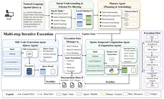
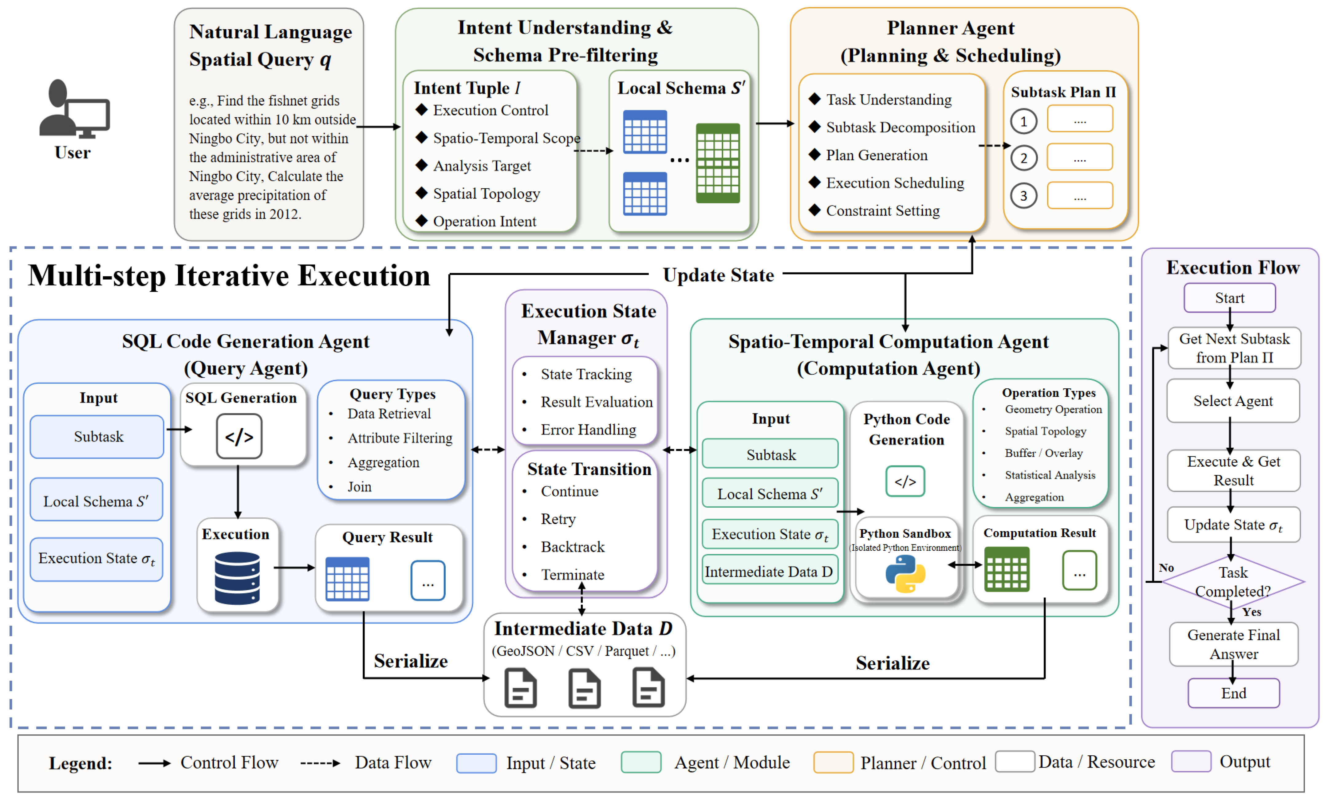
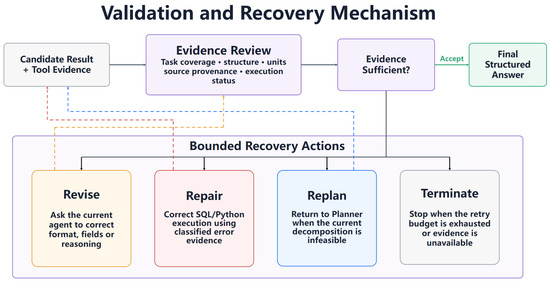
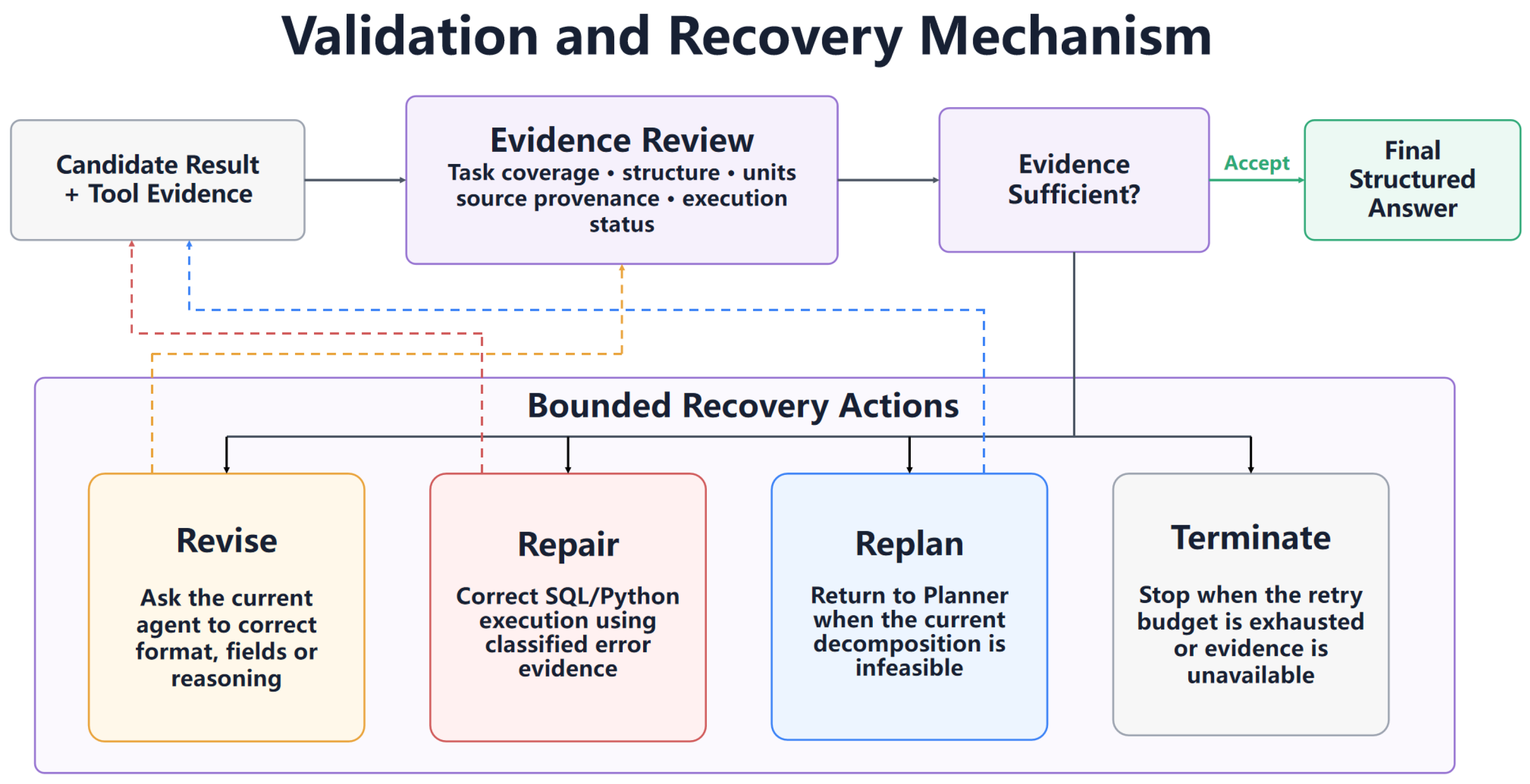
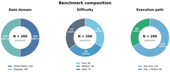
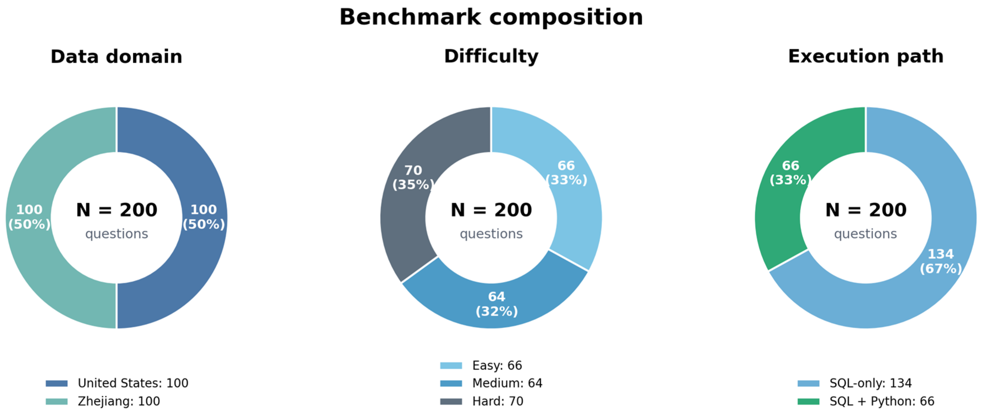
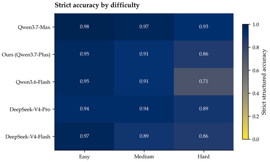
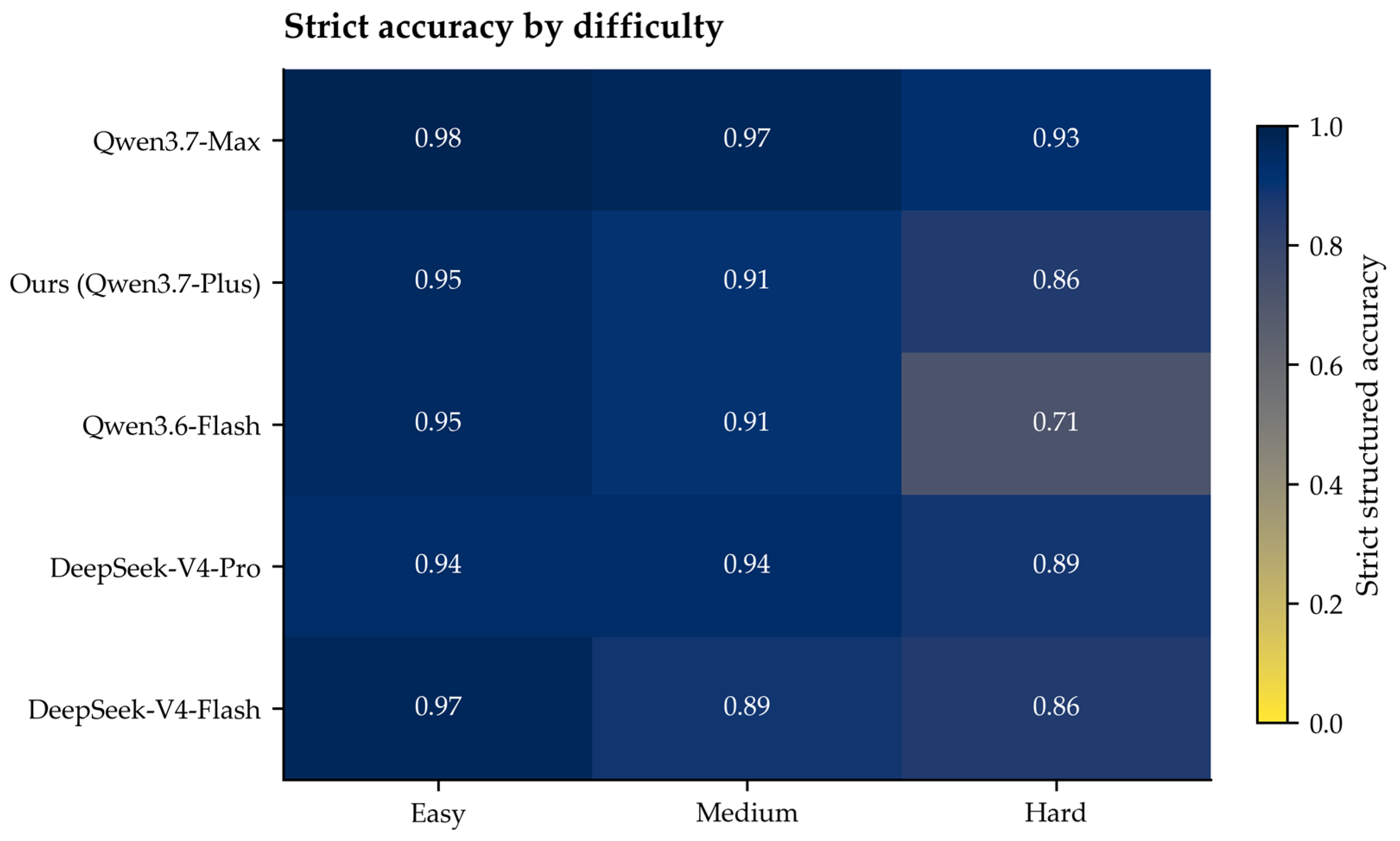
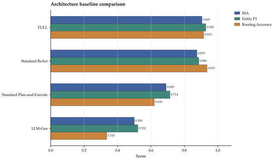
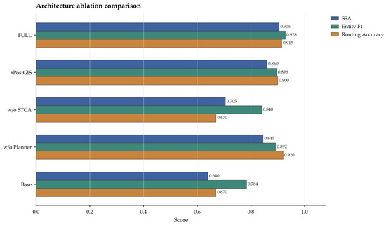
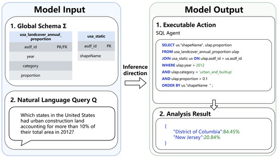
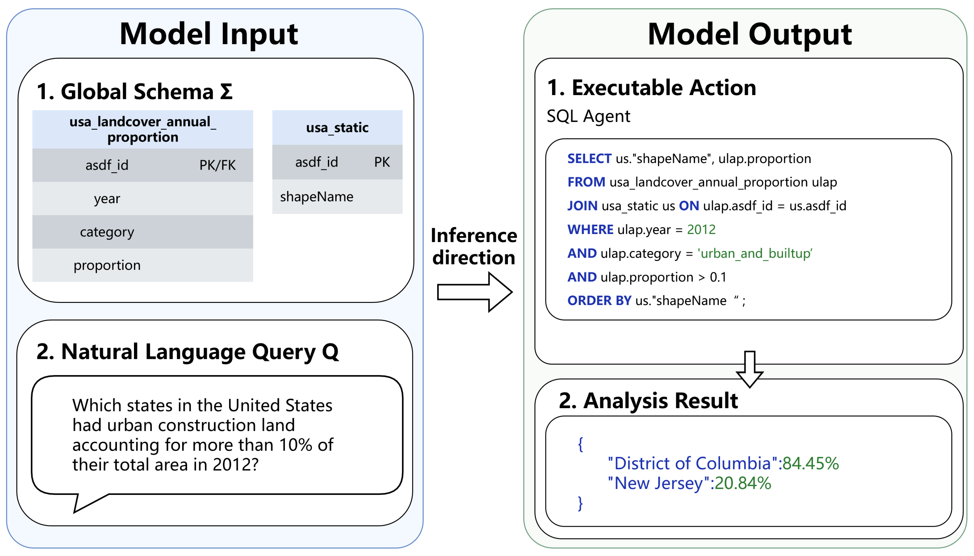
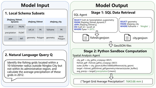
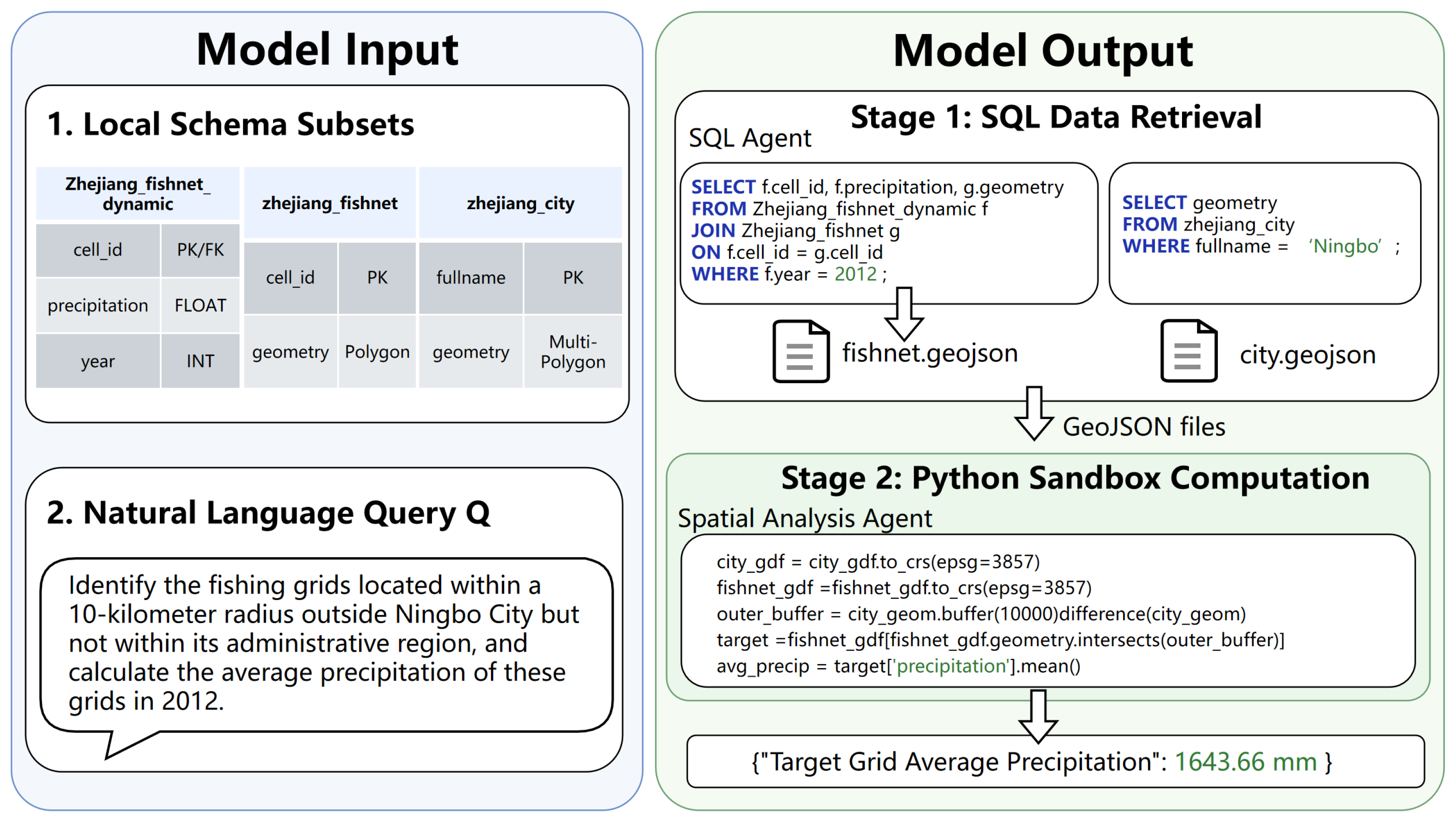

Disclaimer/Publisher’s Note: The statements, opinions and data contained in all publications are solely those of the individual author(s) and contributor(s) and not of MDPI and/or the editor(s). MDPI and/or the editor(s) disclaim responsibility for any injury to people or property resulting from any ideas, methods, instructions or products referred to in the content. |
© 2026 by the authors. Published by MDPI on behalf of the International Society for Photogrammetry and Remote Sensing. Licensee MDPI, Basel, Switzerland. This article is an open access article distributed under the terms and conditions of the Creative Commons Attribution (CC BY) license.