


Abstract
Under rapid urbanization, street crime poses growing challenges to urban safety. Existing studies often treat gray and green spaces as independent variables, limiting the understanding of nonlinear crime patterns and spatiotemporal heterogeneity. Using day–night street crime data from Shanghai between 2010 and 2020, this study applies an interpretable machine learning framework combining CatBoost and SHAP to examine how the coupling of gray–green spatial structures influences street crime. Gray–green spatial morphology is quantified using both MSPA- and Fragstats-based indicators, which are integrated into composite coupling indices. The results indicate that gray–green structural coupling exhibits significant nonlinear and threshold-dependent effects on street crime. Compared with conventional Fragstats metrics, MSPA-based structural indicators demonstrate stronger explanatory power. Theft-specific analysis further indicates that gray-space core–edge structures exhibit higher crime risk at night, with this effect becoming more pronounced in the later period. Across both study periods and day–night contexts, green branch areas (G_BRANCH) consistently show stable inhibitory effects, with the strongest suppression occurring when G_BRANCH values range between 0 and 1.6 and interact with gray core–edge structures (B_CORE and B_EDGE). These findings provide quantitative evidence that gray–green spatial structures function through coupled, nonlinear interactions and offer targeted spatial planning implications for crime prevention in high-density cities.
1. Introduction
1.1. Research Background
Urban safety is a core indicator of sustainable urban development and is explicitly emphasized in the United Nations Sustainable Development Goal (SDG) 11, Sustainable Cities and Communities. In recent years, crime statistics and policy reports (e.g., CCJ, CSEW, and KOSIS) from multiple countries indicate that although overall levels of violent crime have declined in some developed nations, street-based and opportunity-driven crimes continue to persist in urban environments. Previous studies further suggest that these crimes are highly concentrated along specific streets and neighborhood-scale spatial units, posing risks to public safety and resident well-being and potentially contributing to population outflow, declining investment confidence, and weakened urban governance capacity [1,2].
Understanding why these hotspots persist requires situating urban crime within the broader context of contemporary “polycrisis”. Cities in the Anthropocene are increasingly shaped by intersecting socio-economic instability, environmental stress, and governance challenges. These interconnected pressures do not occur independently; rather, they interact across scales and exert continuous systemic pressure on the stability of urban social and spatial systems [3,4,5]. From the perspective of environmental criminology, macro-level stressors do not necessarily lead to crime directly; rather, they reshape the conditions under which crime may occur by influencing the functioning of urban spaces and patterns of routine activities. Consequently, urban crime should not be interpreted as a series of isolated incidents, but as the outcome of interactions between multi-scalar social pressures and localized spatial environments.
Within this framework, crime clustering is often interpreted as the spatiotemporal manifestation of opportunity structures that emerge from routine activity patterns and environmental contexts [6,7]. In other words, crime patterns reflect the spatial opportunity structures generated by everyday activities and environmental conditions at the neighborhood scale. However, most studies treat green or gray spaces around historical crime locations as independent variables and focus on quantity or scale effects of single elements, which limits explanations of nonlinear patterns, contextual dependence, and temporal variation in crime distribution [8,9]. Accordingly, this study conceptualizes gray–green spatial coupling as an integrated and interacting spatial system. Drawing on insights from landscape ecology and environmental criminology, gray–green spatial coupling is defined as the structural, functional, and statistical interplay between built and natural elements within urban environments [10,11,12].
1.2. Theoretical Foundations of Urban Crime Research
Modern environmental criminology seeks to decode the spatial logic underlying criminal events. As activities continuously accumulate perceptible and usable environmental information in space, potential offenders gradually develop experiential awareness of place structure, population movement, and guardianship conditions through repeated exposure. The ‘place knowledge’ unconsciously accumulated in this process influences offenders’ location choice and decision-making [6,7,9,13]. Crime becomes more likely when motivated offenders, suitable targets, and the absence of capable guardians converge within specific spatiotemporal contexts and align with particular crime opportunity structures [7,14]. From a spatial perspective, the design of land use, boundary control, visibility, and accessibility can reshape crime opportunity structures [15,16,17,18]. Overall, crime pattern theory, routine activity theory, and CPTED share a common understanding that crime is a situational decision-making process embedded in routine activities and spatial structures rather than an isolated or irrational act. The spatial distribution of crime fundamentally emerges from ongoing interactions among the physical environment, social structure, and spatial actors. Together, these perspectives emphasize that crime patterns are shaped by spatial opportunity structures embedded within everyday urban environments. However, previous studies suggest that urban crime research still requires further development in structural representation, interaction modeling, and multiscale explanatory frameworks [8,19,20,21,22,23].
As a key spatial unit linking macro urban structure and individual daily activities, streets serve as major carriers of crime risk at the micro scale, and their safety directly shapes public perceptions of urban environments [15,24]. The traditional ‘eyes on the street’ theory emphasizes crime deterrence through natural surveillance and pedestrian activity, yet recent evidence indicates that this suppression effect is not universally effective, especially for purposive users [25,26]. Internationally, studies on urban street crime exhibit marked regional variation. North American studies often focus on opportunity structures and neighborhood vulnerability to examine interactions among street environments, social integration, and crime distribution [27,28,29]. European research empirically shows that well-designed visibility structures contribute to enhanced perceptions of safety [30]. However, highly transparent spaces may induce ‘fishbowl’ or ‘fortress’ effects, thereby increasing potential risks under certain conditions [31]. Low-cost spatial interventions and community organizing curb street violence in resource-poor cities across the Global South [32,33,34]. By contrast, East Asian studies place greater emphasis on integrating qualitative analysis with quantitative techniques [35,36,37]. On the one hand, land-use and multi-source street-view data are increasingly integrated with network analysis, graph representation learning, and machine learning to improve the accuracy of crime risk prediction [24,25,38]. Meanwhile, spatiotemporal dynamics have been analyzed to reveal the heterogeneity and diffusion patterns of different crime types at the neighborhood scale [39,40,41]. However, most models treat environmental factors as isolated predictors, neglecting the interactive effects and spatial coupling of elements within the neighborhood environment.
1.3. Regulatory Effects of Gray–Green Spatial Morphology
Street safety is increasingly recognized as emerging from the interaction between street morphology and surrounding gray–green spatial environments rather than the result of isolated spatial elements. Recent studies show that gray and green spaces indirectly shape guardianship and opportunity structures by regulating psychological states, microclimate, and place-use patterns [29,42,43,44]. Within the spatial opportunity structure perspective, these environmental attributes can be understood as operating through distinct gray and green mechanisms that jointly influence crime risks. For gray spaces (the built environment, including buildings, roads, squares, and various types of artificial impervious surfaces), single built elements have limited explanatory power, but functional juxtaposition at the neighborhood scale significantly increases crime risk and fear [45,46]. Road connectivity and accessibility are generally associated with increased visibility and permeability, thereby suppressing crime in most contexts [47,48]. However, streets with high centrality and traffic potential may also reduce site-selection and escape costs for offenders under certain conditions [49,50]. Moreover, targeted interventions at key anchor places can effectively constrain the spatial range of criminal activities [22,51,52].
By contrast, the regulatory functions of green spaces on street crime are also highly context dependent. Multiple studies find that well-maintained and visually accessible green spaces (natural or semi-natural vegetated areas within urban contexts, including urban forests, tree cover, urban lawns, campus green spaces, sparsely vegetated areas, as well as agricultural land at the urban fringe) reduce fear of crime and suppress various offenses [28,36,53,54]. However, in low-traffic or socioeconomically disadvantaged areas, dense vegetation may obstruct sightlines and reduce visibility, providing concealment for offenders [55,56]. Moreover, moderately enclosed green spaces can reduce criminal propensity or influence decision-making by relieving stress, restoring attention, and promoting prosocial behavior [22,26]. In summary, synthesized evidence suggests that visibility and accessibility constitute the core dimensions through which gray–green spatial environments influence street crime.
1.4. Research Framework and Questions
Empirical evidence indicates that gray and green spaces exert nonlinear and interactive effects on neighborhood crime, varying across crime types and temporal periods [57]. Conceptualized as gray–green spatial coupling, these interactions allow built and ecological elements to jointly reshape crime opportunity structures. Here, spatial structure acts as a contextual buffer, mediating the impact of broader socioeconomic stressors on local street safety rather than serving as an isolated cause of crime [46,47]. Accordingly, integrating these elements into a unified analytical framework to examine their coupling effects has become an important direction for advancing crime research.
However, such theoretical complexity is rarely captured by existing empirical methodologies. As traditional regression approaches (e.g., spatial lag models and geographically weighted regression) generally rely on linear assumptions, their capacity to characterize threshold effects and nonlinear inter-variable interactions remains limited [55] Furthermore, high-performance machine learning models are frequently criticized as ‘black boxes,’ making their outcomes difficult to operationalize for planning and design. Moreover, prior studies in land-use research are often characterized by scale generalization, inadequate modeling of variable interactions, weak explanatory clarity, and overgeneralization of crime types, leading to both convergent and divergent findings. While increasing attention has been paid to gray–green trade-offs [58], comprehensive frameworks that incorporate both as central variables for crime analysis are still scarce. Even where statistical significance is observed for related indicators, explanatory performance typically remains moderate [59,60,61], which is largely attributable to the omission of complex interactions between gray and green spaces.
Addressing these gaps, this study examines street crime in Shanghai during 2010–2020 across daytime and nighttime contexts by applying an interpretable machine learning framework centered on SHAP, aiming to uncover nonlinear response patterns and potential threshold-like transitions of gray–green variables without sacrificing predictive accuracy. Gray–green spaces are treated as a coupled spatial system, and their relative contributions are interpreted through the combined lenses of crime pattern theory, routine activity theory, and CPTED. The following questions are emphasized in this study: (1) Which gray–green configuration indicators are most influential in reducing street crime, and how do they rank in relative importance? (2) Are there significant nonlinear relationships and threshold-like patterns between gray–green characteristics and street crime, and do interaction effects jointly shape the emergence and alleviation of crime hotspots? (3) Do the above associative patterns differ by daytime versus nighttime contexts and across different periods? Through a systematic assessment of the associative effects of gray–green spaces on street crime, this work seeks to offer interpretable empirical support for street safety governance in high-density cities from the standpoint of urban spatial optimization and regeneration.
2. Research Area and Data
2.1. Research Area
This study takes Shanghai as the research area. Situated along the eastern coast of China (31.2304° N, 121.4737° E). As a rapidly urbanized megacity with complex interactions between built and ecological environments, Shanghai offers a typical context for examining gray–green spatial coupling and street crime dynamics. Based on Numbeo (November 2025 update), Shanghai has a low crime index and is macroscopically safe, yet this metric cannot reflect intra-urban crime spatial heterogeneity. Existing research shows Shanghai’s street crime has significant spatiotemporal clustering, concentrating in high-density, high-activity areas [25]. As population density has gradually expanded from the historical urban core toward the inner–outer ring belt, crime hotspots have shown a similar outward extension pattern. In addition to spatial concentration, crime incidents also display clear temporal regularities, with peaks occurring during the morning commuting period (08:00–10:00) and evening activity period (18:00–20:00) [39]. To visualize these dynamics, Figure 1 illustrates the kernel density estimation (KDE) of overall crime across observation periods, the shifting density of theft incidents between the initial (2010–2015) and subsequent (2016–2020) phases, and the 24 h temporal distribution of street crime across both study periods.
Figure 1.
(a) Spatial distribution of overall crime hotspots during the early and later study period based on kernel density estimation; (b) Spatial distribution of theft incidents in the early and later study periods based on kernel density estimation; (c) Temporal distribution of daily crime incidents in Shanghai during the study period.
2.2. Data
Multiple sources of spatial data were integrated in this study, covering street crime, land use, buildings, road networks, nighttime lights, population, and topographic information. The street crime dataset was sourced from China Judgments Online, curated by the Zhang, Y. team in 2025, and made publicly available on Figshare (CC BY 4.0) [62]. Following data preprocessing, samples with incomplete location information, ambiguous crime types, or poor positional accuracy were excluded, resulting in 30,044 valid street crime cases mainly involving theft, robbery, and snatching from 2010 to 2020 (14 categories in total; Table A1, Appendix A), which served as the dependent variable.
Land-use information was obtained from GlobeLand30 (2010, 2020), with a spatial resolution of 30 m and consistently high classification accuracy (overall accuracy: 80.33–85.72%). The road network was extracted from OpenStreetMap (OSM) historical data (OSM history extracts) for the years 2014 and 2020 to match the two observation periods., while points of interest (POI) data were acquired through the Amap open-platform API. Nighttime light data were obtained from the open dataset provided by Chen [63], with a spatial resolution of 15 arc-seconds (~500 m). Population density data for 2010 and 2020 were sourced from WorldPop, at a spatial resolution of 100 m.
All datasets were projected to a unified coordinate system and analyzed at a consistent spatial scale. Population density, nighttime light intensity, building density, and road-network indicators were included as control variables representing human activity intensity and built-environment characteristics to mitigate omitted-variable bias; their specific effects are not discussed in detail (Table 1).
Table 1.
Data sources and temporal alignment of variables used in the study.
2.2.1. Development of Composite Indicators for Gray–Green Space
To investigate the nonlinear and interaction effects of gray–green space on street crime, this study established a hierarchical composite indicator framework. The framework comprises four phases: (1) data acquisition and integration, (2) spatial structural characterization using MSPA, (3) model construction via CatBoost, and (4) interpretability analysis based on SHAP values. The model aims to reveal interpretable spatial associations between gray–green spatial structures and crime risk rather than purely predictive crime forecasts.
In Phase 1, street crime records obtained from China Judgments Online were treated as the dependent variable, with crime points aggregated into 3000 m × 3000 m grid cells using spatial join (one-to-one) to obtain the cumulative number of crimes per cell, with each incident contributing equally (weight = 1). Sensitivity tests using 2 km and 1 km grids show that model performance and main spatial relationships vary, not adopted (Appendix B and Appendix C). Global Moran’s I was calculated to test spatial dependence prior to modeling (Table A4). In line with existing research [9], daytime and nighttime periods were defined using 06:00 and 18:00 as cut-off points, and Shanghai street crime data corresponding to the two observation periods (2010–2015 and 2016–2020) were screened and logarithmically transformed. Both dependent and independent variables were harmonized to an identical spatial resolution to maintain consistency in analysis.
Subsequently, representing Phase 2, spatial structural attributes of gray and green space subsystems were quantified by integrating land use/land cover (LULC) data with environmental variables. FRAGSTATS metrics combined with MSPA were employed to describe spatial coverage, fragmentation levels, connectivity patterns, and morphological configurations. Widely applied FRAGSTATS indicators such as CA, ED, and LSI were used to assess patch scale, morphological complexity, and fragmentation. MSPA classifies urban green space into seven morphological types: Core, Edge, Perforation, Bridge, Loop, Branch, and Islet. Types to capture morphological features of gray–green space. A total of 64 candidate indicators representing gray–green space were derived.
Regarding Phase 3, key indicators were identified through correlation testing, and indicator weights were determined using the CRITIC method to construct composite indices for gray space (BMSF) and green space (GMSF). The selected indicators were further aggregated into eight composite gray–green space variables, which were used as the main explanatory factors in the models. An optimal CatBoost model was identified via multi-model comparison to capture complex and non-linear associations.
Lastly, as Phase 4, SHAP was introduced to explain and visualize the contributions, nonlinear thresholds, and interaction effects of gray–green composite indicators. The proposed framework establishes an end-to-end process from indicator development to interpretation. To further clarify the computational workflow of the modeling and interpretability procedures, the integrated CatBoost–SHAP framework is summarized in Appendix F Algorithm A1. This framework contributes a methodological approach for quantifying gray–green space structures and evaluating their safety implications in high-density urban contexts.
2.2.2. Overview of MSPA and FRAGSTATS Metrics
MSPA is used to describe structural categories of gray–green space based on spatial topology and has been extensively applied to green infrastructure studies, ecological connectivity evaluation, and analyses of urban green space patterns [64,65]. In this research, MSPA analysis was performed using binarized gray–green space maps, where green space was treated as the foreground and gray space and other land uses as the background, with the definitions inversely applied in gray space analysis. Edge width parameters were standardized based on raster resolution to maintain consistency in structural recognition across different spatial units.
Regarding landscape pattern quantification, based on research on landscape pattern–ecological process linkages [66,67], 25 FRAGSTATS indicators were selected across area scale, morphological complexity, and fragmentation dimensions to describe landscape characteristics of gray and green spaces and to establish a comprehensive gray–green indicator framework (Figure 2).
Figure 2.
Workflow of this research.
2.2.3. Pearson Correlation Analysis
To ensure the independence of the integrated gray–green spatial indicator system, a multicollinearity test was conducted on a total of 50 gray and green landscape indicators across the two five-year periods. All indicators were first standardized to eliminate dimensional differences. Subsequently, pairwise correlations among indicators were examined using the Pearson correlation coefficient [68]. When the absolute value of the correlation coefficient exceeded 0.9 ( > 0.9), the indicators were regarded as highly collinear, and redundant variables were removed accordingly. As a result, 14 gray space indicators and 13 green space indicators were retained for subsequent analyses in each period (Figure 3).
Figure 3.
Correlation coefficient graph.
To further mitigate the potential interference of strong intercorrelations among FRAGSTATS-derived landscape metrics on the subsequent CRITIC weight calculation, Pearson correlation analysis was additionally applied for indicator screening. It is widely used to assess linear variable associations [41].
The Pearson correlation coefficient is calculated as follows:
In the equation, denotes the Pearson correlation coefficient between indicators; , represent the two gray–green FRAGSTATS indicators to be screened; refers to the sum of the products of the corresponding observed values of the two indicators; , denote the sums of all observed values of each indicator, respectively; represents the number of observations; and , indicate the sums of squared observed values for each indicator. The resulting correlation values were used for subsequent indicator screening and the construction of composite indices.
2.2.4. Composite Index Calculation
Based on the indicator screening results, 14 gray-space indicators and 13 green-space indicators were selected as inputs, and the CRITIC method was applied to determine the objective weights of each indicator.
In this method, indicator variability is measured by the standard deviation, where a larger standard deviation indicates a greater degree of dispersion and a higher amount of information contained in the indicator. Indicator conflict is quantified using the correlation coefficient. When an indicator shows weaker correlations with other indicators, it implies lower information redundancy and a greater contribution to the overall evaluation system.
By integrating both indicator variability and conflict, the CRITIC method calculates the information content of each indicator and determines its corresponding objective weight in the composite index. This method avoids excessive weight concentration caused by large variances in individual indicators, thereby enhancing the stability and representativeness of the composite index, and making it well suited for multidimensional and highly correlated urban gray–green space indicator systems.
The calculation formula of the CRITIC method is as follows:
In this formulation, denotes the objective weight of the th gray–green space indicator in the composite index system, reflecting its relative importance in characterizing urban gray–green spatial structures and their spatiotemporal variations. Where represents the information content of a given gray- or green-space indicator, capturing its variability across units and its conflict with other indicators based on correlation; higher values of indicate greater discriminative power and a more significant role in the composite indicator construction. denotes the total information content of all indicators and is used for weight normalization to ensure that the sum of weights equals one, thereby improving the comparability and integrability of indicators in composite index construction. The derived weights were subsequently used to construct gray–green space composite indices and served as explanatory variables in the crime analysis.
2.2.5. SHAP Explanation Method
To reveal the relative contributions and interaction effects of different landscape indicators on crime intensity, this study employs the SHAP (Shapley Additive Explanations) method to interpret the outputs of the CatBoost regression model. Grounded in game theory, SHAP provides consistent and locally accurate feature attributions for each prediction sample (i.e., the predicted crime risk for each spatial grid) [69]. Here, ‘features’ refer to various landscape indicators or specific street facility attributes, enabling a quantitative assessment of the marginal contribution of each explanatory variable to the model-estimated crime propensity.
SHAP calculation formula:
Specifically, denotes the th landscape indicator (e.g., the proportion of green space or the distribution of gray space) and its average contribution to the predicted crime intensity; represents the feature set consisting of gray–green spatial indicators; refers to any subset of these variables; and and denote the model prediction based on the feature subset and on the subset augmented by indicator , respectively. After the indicator weights are determined, eight composite indicators are constructed by integrating four pairs of gray–green spatial indicators.
Here, denotes the th composite index quantifying gray–green space ( = 1, 2, …, 8); r represents the number of indicators retained after final selection; and refers to the calculated values of the sub-indicators constituting the three categories of composite indices, namely B/GCI, B/GACI, and B/GFC.
2.3. Model Evaluation
To assess the influence of eight composite indicators on crime intensity, a multi-model comparative approach was employed to select the most suitable predictive model. The dataset was randomly split into training (70%) and testing (30%) subsets, where the training data was used for model training and hyperparameter optimization, and the testing data was used to assess model generalizability. To further evaluate model robustness, a 10-fold cross-validation procedure was conducted (Appendix D). The dataset was randomly divided into ten folds, and the model was trained and validated iteratively across these folds. The comparative analysis involves Multiple Linear Regression (MLR), SVR, Random Forest, XGBoost, LightGBM, and CatBoost models. The optimal model is determined by jointly assessing model performance on the testing set using Test R2 and RMSE. The findings show that CatBoost outperforms other models in terms of explanatory capacity and stability across temporal scales and diurnal contexts, leading to its selection as the final analytical model. Table 2 presents the prediction performance of each model across four scenarios, namely daytime and nighttime periods in 2010–2015 and 2016–2020.
Table 2.
Performance comparison of CatBoost and benchmark models.
In general, linear models showed limited explanatory capability, while ensemble models based on decision trees achieved superior performance in most contexts. Notably, CatBoost obtained relatively high R2 and low RMSE under most temporal and day–night settings, demonstrating robust generalization ability. CatBoost (Categorical Boosting) represents an ensemble learning approach derived from Gradient Boosting Decision Tree (GBDT) frameworks. In addition to high prediction accuracy, CatBoost enhances training stability and generalization, and is especially effective when sample sizes are small and nonlinear interactions among features are pronounced. By effectively identifying high-order nonlinear dependencies and exhibiting strong robustness to noise and outliers, the model shows good adaptability in urban environment–crime modeling [70,71]. Accordingly, CatBoost was adopted as the final model for examining the associations between gray–green spatial composite indicators and crime rates.
CatBoost calculation formula:
where denotes the ensemble prediction at iteration , is the prediction from the previous iteration, represents the newly fitted decision tree, is the learning rate controlling the contribution of each tree. The input vector represents the set of explanatory variables, including the gray–green spatial composite indicators and other environmental variables used in this study, and is the total number of boosting iterations. Through sequentially adding weak learners, the model progressively reduces prediction errors and enhances predictive accuracy.
3. Results
3.1. Overview of Crime Distribution
During the period 2010–2020, street crime in Shanghai demonstrated significant heterogeneity across both temporal and spatial dimensions. Figure 4a,b present the kernel density estimation results of overall crime hotspots during the early observation period (2010–2015) and the later period (2016–2020), illustrating the changes in spatial distribution patterns. During the early period, crime hotspots were mainly concentrated in the central urban districts, particularly in the ZB and JA districts and their surrounding areas. The spatial distribution exhibited a clear core–periphery pattern, with dense clusters located in the urban core and relatively dispersed activity in the peripheral areas. Although the overall number of recorded crimes during the early years was relatively limited, spatial concentration around major urban centers was already evident. In the later period, the primary hotspot areas in JA and XH districts remained relatively stable. However, the total number of crimes gradually increased before declining after 2015. During 2019–2020, the total number of recorded crimes reached its lowest level during the study period. Despite the reduction in the overall number of incidents, the spatial extent of crime distribution expanded over time, suggesting a gradual outward diffusion of crime risk from the traditional urban core to surrounding districts.
Figure 4.
(a) Spatial distribution of overall crime hotspots during the early study period based on kernel density estimation; (b) Spatial distribution of overall crime hotspots during the later study period based on kernel density estimation.
As illustrated in Figure 5, temporal patterns also changed significantly during the study period. In detail, daytime crime reached its highest share in 2010 (0.705), showing the greatest disparity relative to nighttime crime (0.410). Such a daytime-dominant structure remained stable for about six consecutive years. Conversely, the proportion of nighttime crime peaked in 2019–2020 (0.652), reflecting a significant transformation in temporal crime patterns. The total number of crimes exhibited a pattern of rising first and then declining over time. Two periods, namely 2013–2014 and 2018–2019, showed the most substantial fluctuations. Among different crime categories, theft remained the dominant crime type (over 70%). Furthermore, as shown in Appendix A (Table A1), theft displayed a notable temporal shift. Daytime theft incidents decreased slightly (from 5365 in 2010–2015 to 4813 in 2016–2020) but a substantial increase at nighttime (from 4281 to 8637). Compared with other crime types such as robbery, fraud, and snatching—which generally declined or fluctuated at relatively low levels—theft exhibited a much larger scale and a clearer shift toward nighttime concentration.
Figure 5.
Temporal differences in crime distribution in Shanghai between the two observation periods (2010–2015 and 2016–2020).
3.2. Spatial Feature Indicators
Figure 6 presents the spatial characteristics of the eight composite indicators together with the variations in weights across their constituent sub-indicators. At the city scale, UBS and UGS display a clear spatial complementarity in their distribution patterns. In terms of weighting structure, the eight composite indicators remain relatively stable between the two observation periods, yet notable differences in internal composition are observed. For green space indicators, the morphological structure factor (GMSF) is primarily driven by the CORE component across both periods, accounting for 65% and 60% of the total weight, respectively. This result suggests that green space core zones remain the dominant component of the urban green space pattern. By comparison, LOOP and ISLET maintain persistently low weights, accounting for roughly 1% and 3%, respectively. This indicates that fragmented green spaces have a limited contribution to the overall structural characterization. The weight composition of gray space indicators, however, exhibits substantially greater variability. Specifically, the CORE element of the BMSF factor rose sharply in importance, increasing from 16% in the earlier period to 66% in the later period. This change indicates a morphological transition of built-up areas from dispersed layouts to more core-oriented and continuous forms. In summary, gray space experienced notable structural restructuring between the two temporal cross-sections, while green space configurations remained comparatively stable. These differences in spatial patterns and structural changes between gray and green spaces form a critical spatial foundation for examining their coupled influences on crime.
Figure 6.
Spatial characteristics of eight comprehensive indicators and the weights of their sub-indicators across both observation periods.
3.3. Analysis of CatBoost Model Results
3.3.1. Analysis of Contribution Level Results
In the research process, the comprehensive indicator model was applied, and it was found that the 14 indicators of BMSF and GMSF (i.e., B_GMSF) play a relatively larger role in explaining variations in crime risks compared with the 64 indicators jointly constructed by Fragstats and MSPA. Among these indicators, the B_GMSF set contributed 48.6% to 50.5% to the daytime crime risks and 49.9% to 55% to the nighttime crime risks across both observation periods, and these two contribution dimensions dominated the variations in day-night crime risk between the two temporal cross-sections. As indicated in Table 3, compared with the 64-indicator comprehensive model, the morphological structure model achieved an explanatory power of over 65% for the day-night crime risks in both study periods, with its explanatory power for the nighttime crime risks rising by 21.7% during the initial 2010–2015 period. Although performance varies across periods, MSPA was selected not for its predictive advantage but for its ability to explicitly capture spatial morphological structures, which better aligns with the study’s objective of representing fine-scale spatial heterogeneity. Therefore, the subsequent analysis focuses on the internal structure of the B_GMSF.
Table 3.
Performance metrics of the CatBoost model based on the gray–green space landscape hierarchy configuration index and structural unit hierarchy MSPA index.
Pearson correlation analysis was applied to the pooled daytime and nighttime data across both observation periods to verify the relationships among gray–green spatial morphology indicators. The findings reveal a shift in dominant crime determinants between the two temporal cross-sections, from suppression effects associated with green space indicators in the initial 2010–2015 period to inducement effects driven by gray space indicators in the subsequent 2016–2020 period. In particular, gray and green morphological structure indicators exhibit strong negative correlations (r = −0.813 to −0.684, p < 0.05), reflecting a pronounced trade-off in spatial arrangement. A positive association is identified between gray space indicators and crime risks (r = +0.268 to +0.768), while green space indicators consistently display negative correlations with crime risks (r = −0.507 to −0.603).
Figure 7 illustrates the relative contributions of specific gray–green spatial structure (B/GMSF) indicators to crime risks. The gray space components (B_CORE, B_ISLET, B_PERFORATION, B_EDGE, B_LOOP, B_BRIDGE, B_BRANCH) consistently dominate contributions during both day and night across both observation periods, with shares of 59.9% and 63.2%. Notably, the gray core zone (B_CORE) represents the most critical indicator, with contribution levels of 37.3% and 43.9%. In the daytime period, the largest contribution shifts occur in the gray core area (B_CORE, −6.6), followed by the green core area (G_CORE, +5.3) and the gray edge area (B_EDGE, −1.6). In contrast, nighttime changes are most evident for the gray core area (B_CORE, −4.7), the green core area (G_CORE, +3.4), and green islet patches (G_ISLET, +2.6). The gray edge area shows the greatest stability and relatively high contribution levels, with values of 6.8% and 9.6%.
Figure 7.
Stacked area map of the contribution of gray–greenstructural indicators (B/GMSF) to Shanghai’s daytime and nighttime crime risks across the two observation periods (2010–2015 and 2016–2020).
3.3.2. Analysis of SHAP Distribution Patterns
Figure 8 further illustrates the heterogeneity in effect direction and magnitude across different MSPA structural units of the B/GMSF indicators. While MSPA-identified green spaces show an overall inhibitory effect on street crime, this composite outcome masks pronounced internal heterogeneity among structural units.
Figure 8.
The impact of 14 indicators based on MSPA structural units on the intensity of daytime and nighttime street crime risks across the two observation periods.
First, in terms of effect magnitude, B_CORE and B_EDGE from gray space show strong positive relationships with G_CORE, representing the core–edge structure of green space. During both daytime and nighttime across both observation periods, these indicators exert positive effects between +0.2 and +2.5, with peak values detected at night during the initial 2010–2015 cross-section. In contrast to the increasing positive effects of gray space core–edge zones, the positive influence of green space core areas on crime risks declines in the subsequent 2016–2020 period.
In terms of suppression, G_BRANCH in green space exhibits the most consistent and significant inhibitory effect on crime risks across both observation periods. The negative impact of G_BRANCH ranges between −1.1 and +0.9, particularly showing stronger effects on street safety in localized nighttime settings during the subsequent 2016–2020 period. Negative correlations with crime risks are likewise observed for B_BRANCH and G_LOOP. While B_BRANCH and G_LOOP show comparable low SHAP value ranges (−0.3 to +0.4 and −0.2 to +0.3, respectively), the overall contribution of the former is greater.
Regarding inducement patterns, B_ISLET exhibits a significant increase in nighttime contexts, with high SHAP values ranging from +0.2 to +0.5. By contrast, the positive influence of green space indicators such as G_CORE and G_ISLET generally declines. With respect to synergy, G_ISLET and B_ISLET show parallel positive effect trends on crime risks across daytime and nighttime (+0.1 to +0.7), transitioning from green-dominated to gray-dominated influence. In contrast, although G_BRIDGE and B_BRIDGE exhibit similar ranges (−0.4 to +0.6), their effects shift from jointly positive in the early stage to gray space–dominated negative effects in the later stage.
3.3.3. Threshold Response Characteristic Analysis
Using MSPA indicators at the structural morphological level, PDP plots further illustrate the nonlinear threshold responses of key gray and green spatial structural units that rank among the top three in importance (Figure 9a–d). The results reveal pronounced differences in threshold patterns across crime types, time periods, and diurnal contexts, highlighting the internal heterogeneity and temporal evolution of gray–green spatial structures.
Figure 9.
Threshold comparative responses of B_GMSF indicators to the comprehensive indicator of 14 types of diurnal street crimes and theft crime intensity across both observation periods. (a) Threshold responses of B_GMSF indicators to the diurnal thresholds of the comprehensive crime indicator, 2010–2015; (b) Threshold responses of B_GMSF indicators to the diurnal thresholds of the comprehensive crime indicator, 2016–2020; (c) Threshold responses of B_GMSF indicators to the diurnal thresholds of the theft crime indicator, 2010–2015; (d) Threshold responses of B_GMSF indicators to the diurnal thresholds of the theft crime indicator, 2016–2020.
For the comprehensive indicator of 14 types of diurnal street crimes (Figure 9a,b), the gray space core area (B_CORE) consistently exhibits a stable positive influence. The SHAP values represent the marginal contribution to the logarithm of crime risks. Specifically, an increase of two standard deviations (0 to +2) in B_CORE is associated with an approximate 3.2–3.5% proportional rise in crime intensity. In the 2016–2020 period, the marginal growth of crime rates gradually slows once the B_CORE threshold approaches approximately 4 under both diurnal conditions, indicating a forward shift (earlier saturation) compared with the higher threshold observed in the initial 2010–2015 cross-section (≈6).
When focusing specifically on theft crimes (Figure 9c,d), the overall importance ranking and directional effects of key indicators remain largely consistent with those observed for the comprehensive crime model, suggesting that the dominance of B_CORE is not solely driven by the high proportion of theft incidents. However, the threshold response patterns become more differentiated. In particular, the gray space edge area (B_EDGE) demonstrates a pronounced inter-period shift. During the initial 2010–2015 cross-section, theft-related SHAP values decline sharply once the B_EDGE standard deviation exceeds approximately 1.5, indicating a suppressive threshold effect. By contrast, in the subsequent 2016–2020 period, theft risk increases rapidly beyond the same threshold, especially during nighttime periods, with SHAP values reaching up to 1.65.
Compared with gray space structures, the green space core area (G_CORE) exhibits a distinct moderating role in theft-related crime dynamics. Across both daytime and nighttime periods from 2010 to 2020, G_CORE shows a stable crime-suppressing interval within the lower standard deviation range (0–5), a pattern that is less evident in the comprehensive crime model.
3.3.4. Characteristic Analysis of Interaction Effect
Interaction effects between gray and green spatial structural units further elucidate the spatial overlay effects underlying crime risk. In general, high SHAP values (>1.2) for daytime and nighttime crime risks across both observation periods are concentrated in conditions where gray or green core areas (B_CORE, G_CORE) exhibit high values (>+8), suggesting that core structures set the upper limit of crime risk in coupled states.
Across both observation periods, interactions (coupling) between the gray core area (B_CORE) and the green core area (G_CORE) are characterized by a green-space-dominated suppressive effect. Under conditions where the gray space core area exceeds 8 and the green space core area remains below 2, both daytime and nighttime crime risks rise markedly, with SHAP values above 1.25. The effect is particularly evident in both daytime and nighttime during the initial 2010–2015 period. The results indicate that within highly concentrated built environments, undersized and isolated green core structures exhibit reduced regulatory capacity and may increase crime risk because of poor accessibility or visual blockage.
Conversely, interactions between the gray edge area (B_EDGE) and the green core area (G_CORE) display more complex nonlinear patterns. In the 2010–2015 period, combinations of elevated B_EDGE (0.5–2.5) with G_CORE values ranging from 0 to +6 consistently demonstrate strong crime suppression during both day and night. Elevated crime SHAP values (1.25) are primarily concentrated in structural configurations featuring strong green cores and weak gray edges. In the subsequent 2016–2020 period, this structural pattern exhibits a markedly higher risk profile, especially as G_CORE decreases to the 0–2 interval, with crime SHAP values within B_EDGE rising above 0.6, reflecting a shift from inhibitory to inducing effects between the two cross-sections. The interaction characteristics are especially evident in nighttime crime patterns. In the 2016–2020 period, the influence of gray space structures on nighttime crime risks is generally stronger.
Nevertheless, G_BRANCH demonstrates consistent and effective inhibitory effects (0 to +1.6) under various gray space combinations, including B_CORE values of 0–+4 or B_EDGE values of 0–+1. In addition, interactions with gray edge areas produce stronger suppression than those with gray cores (2016–2020 nighttime), further supporting the buffering effect of green extension structures in settings.
4. Discussion
4.1. Temporal Evolution of Street Crime Risk Types
This study divides the observation period into two stages (2010–2015 and 2016–2020) and distinguishes daytime and nighttime contexts to examine how long-term urban spatial evolution and accumulated governance capacity reshape street-crime risk. Although overall crime levels declined in both study periods, the spatial organization of crime risk and its dominant structural components changed substantially. In both periods, the core structures of gray and green spaces (B_CORE and G_CORE) consistently emerged as key spatial elements shaping street-crime risk (Figure 7 and Figure 8).
During the earlier period (2010–2015), gray-space environments characterized by intensive development and frequent facility use played a dominant role, particularly within core areas and adjacent edge zones during daytime. This pattern reflects a typical core–edge exploration process under routine activity conditions, in which offenders’ repeated movements between activity nodes gradually expand opportunity awareness from core areas into surrounding edge zones. Large and structurally continuous green-space core patches showed stronger crime-suppressing associations for certain offenses during nighttime (Figure 9c). However, from a CPTED perspective, insufficient natural surveillance in centrally located and morphologically pronounced cores may offset these benefits, leading to localized exposure risks. In the later period (2016–2020), crime risk became more concentrated in dense built-up areas at night and their surrounding zones, where the core–edge structure of gray space showed stronger spatial concentration effects. This finding aligns with previous research suggesting that edge areas may be underestimated in prevention systems, as population mobility, temporal overlap of activities, and relatively weaker management increase the likelihood that these locations enter offenders’ experiential awareness space [6,72]. Meanwhile, linear spatial units formed by green-space branch structures assumed a more prominent crime-suppressing role during nighttime (Figure 8).
These shifts reflect the broader dynamics of city-building, where changing land-use priorities and evolving social rhythms reshape the crime-environment nexus through processes such as economic restructuring, expanding nightlife economies, and fragmented mobility patterns. From a spatial-morphological perspective, research findings provide temporally differentiated empirical support for crime pattern theory. While objective criminal opportunity is a necessary condition, the actual occurrence of crime is governed by an offender’s internalized cognitive template for offending—comprising their specialized knowledge, perception of opportunities, and varying degrees of spatial familiarity. This suggests that awareness space is not static but is dynamically activated under specific spatiotemporal conditions [7,9,20].
4.2. Differences in Structural Indicators of Gray–Green Spaces
Gray–green spatial structures exert asymmetric effects on crime (Figure 10). As urbanization progresses, the inducement linkage of deep green-core patches (G_CORE) weakens over time, whereas the crime-promoting linkage of gray cores (B_CORE) increases. Metrics for gray space that reflect aggregation and reinforced boundaries (B_CORE, B_EDGE) show persistent positive correlations under varying conditions, evidencing marked inducement tendencies; conversely, the inhibitory role of green space is less contingent on aggregation and is primarily driven by branch and edge arrangements. Significantly, G_BRANCH consistently demonstrates the strongest and most stable suppressive links across all settings. This effectiveness stems from the fact that such layouts enhance spatial visibility and use frequency; the spatial permeability of green branches structures improves sightlines and natural surveillance capacity. Thus, in dense urban environments, enhancing green-space visibility and structural accessibility can significantly reduce the perceived of crime opportunities and thereby weaken neighborhood-level risk patterns [72,73].
Figure 10.
Interaction effects among factors in gray–green structural indicators (B/GMSF).
In addition, threshold-based analyses (Figure 9) focusing on theft crimes further reveal the temporal reinterpretation of gray–green spatial structures. Although theft accounts for more than 70% of total crime incidents, its threshold response patterns do not simply dominate the overall crime pattern. Instead, they expose crime-type-specific and time-sensitive opportunity effects that remain latent in the comprehensive model. Specifically, gray space edge areas (B_EDGE) evolved distinctly from transitional, unstable activity spaces to high-exposure, high-activity opportunity settings with inadequate nighttime governance, with fragmented, weakly integrated edges curbing crime opportunity accumulation in the early stage, whereas the same threshold triggered a sharp surge in theft risk—especially at night—in the later period, driven by intensified functional mixing and extended activity hours that turned gray edges into effective opportunity amplifiers. These day–night asymmetries and inter-period variations reflect broader transformations in urban temporal organization rather than simple daily mobility rhythms. By capturing these shifting dynamics, these findings offer a more granular foundation for developing spatially differentiated and temporally responsive planning strategies, moving beyond the principle-based recommendations of previous studies.
4.3. Coupling and Correlation of Gray–Green Spatial Forms
The interaction results between B_EDGE (gray edge) and G_CORE (green core) reveal a clear inter-period reversal in their associative effects. During 2010–2015, spatial configurations characterized by high G_CORE and low B_EDGE showed significantly positive SHAP values, whereas low G_CORE combined with high B_EDGE produced negative effects. This suggests that, in the initial 2010–2015 period, environments with a clearer building boundary and smaller green-core structures tended to exhibit lower crime risk, likely because stronger boundary definition constrained accessibility while limited dense vegetation maintained relatively open sightlines. Conversely, areas with a higher proportion of core green-space structures and weaker spatial boundaries tended to generate crime opportunities. In the subsequent 2016–2020 cross-section, this relationship reversed, with urban green-space structures characterized by stronger core morphology in central areas no longer amplifying crime opportunities but instead contributing to risk suppression. These findings indicate that the influence of spatial structural variables on crime is highly context-dependent, being functionally reinterpreted between the two periods reflecting differences in urban governance capacity, spatial use patterns, and regulatory continuity evolve. This observation aligns with van Sleeuwen [9], suggesting that these interactions reflect the joint influence of spatial accessibility and environmental visibility on the formation of crime opportunities.
Moreover, significant cross-category synergistic effects are observed for islet-related indicators (B/G_ISLET). The increasingly aligned inducing effects of B_ISLET (gray islets) and G_ISLET (green islets) evolve from green-dominated influences in the initial stage to gray-dominated influences in the subsequent stage, suggesting that the combined presence of fragmented gray and green patches may heighten spatial ambiguity and governance gaps, simultaneously weakening environmental visibility and producing irregular accessibility pathways that expand potential opportunity structures for offenders. Conversely, the later-stage synergistic suppression associated with B_BRIDGE and G_BRIDGE during the 2016–2020 period indicates that the effective integration of fragmented elements through structured connectivity networks can significantly enhance spatial visibility and accessibility, thereby strengthening natural surveillance effects. These findings suggest that spatial fragmentation itself does not inherently generate crime risk; rather, risk emerges when spatial discontinuities fail to mediate broader systemic pressures. However, integrating fragmented gray–green elements into structurally continuous networks, urban spatial morphology can function as a contextual buffer that mitigates the cascading effects of multi-scalar urban stressors.
5. Conclusions
5.1. Research Contributions
This study advances the methodology and empirical understanding of urban environmental criminology by integrating MSPA-based structural analysis with a complexity-oriented framework.
First, this study advances the measurement of urban crime-related environments by shifting from quantity-based indicators to a structural representation of gray–green configurations. Unlike traditional studies relying on LULC, NDVI, we introduce MSPA to construct a refined indicator system. This provides a transferable methodological framework for analyzing built-environment structures in crime-related research. Our findings reveal that G_BRANCH (green corridors/branches) maintains a significant and stable crime-suppressive effect across multiple scales (1–3 km) and diurnal contexts. This suggests that the “connectivity” of green networks—realized through strategies like “pocket parks,” “linear greenways,” and “distributed small-scale greenery”—is more critical for urban safety than mere green coverage.
Second, this study reveals the complex coupling effects and threshold patterns between gray–space morphology and crime across temporal and type-specific contexts. A key discovery is the evolving role of gray structures: compared to the 2010–2015 period, B_CORE in 2016–2020 showed a higher efficiency in inducing crime, reflecting the concentration of “motivated offenders” and “suitable targets” in high-density urban hubs. Conversely, B_EDGE demonstrated a suppressive tendency, likely due to stronger territoriality among local residents and lower anonymity compared to cores. However, this crime-inhibiting capacity gradually contracted over time. This shift was potentially driven by increased social anonymity resulting from population inflow and the enhanced permeability of urban spaces due to facility improvements, which may have weakened local territorial control and informal surveillance. Notably, for theft-related crimes, edge areas transitioned from crime-buffering zones into potential generators under changing socio-spatial conditions. Furthermore, interaction analysis further confirms that G_BRANCH effectively mitigates the crime risks associated with both B_CORE and B_EDGE.
Third, building on classic frameworks (e.g., RAT, Crime Pattern Theory, and CPTED), this study situates environmental criminology within a broader “polycrisis” perspective. The findings suggest that spatial crime patterns are shaped not only by dynamic environmental cues but also by interactions among urban subsystems under evolving socioeconomic pressures. Identified threshold effects further indicate that gray–green morphology may function as an adaptive spatial structure with “contextual buffering” properties, through which macro-level pressures may translate into micro-level crime risks, consistent with complexity-oriented urban processes.
5.2. Planning Implications and Policy Relevance
The findings indicate that gray–green spaces possess substantial functional adaptability, with their moderating effects on street crime varying across the two observed stages of rapid urban transformation and shifts in governance intensity. Based on a comparative analysis of two discrete periods of daytime and nighttime street crime in Shanghai, isolated interventions targeting only ‘green’ or ‘gray’ spaces fail to deliver consistent and reliable safety performance. By comparison, synergistic planning approaches based on the structural coupling between gray and green spaces offer higher practical applicability and policy value for cities navigating similar polycrisis-driven instabilities.
At the micro-level of targeted spatial intervention, the nonlinear relationships identified between gray–green spatial indicators and crime risk provide a basis for evidence-based spatial threshold management. The empirical results suggest that maintaining green branching structures within a moderate range (approximately +0.05–+0.4) produces stronger crime suppression effects, particularly when interacting with built cores and edge zones of appropriate scale. In practice, this implies that small-scale green structures—such as pocket parks, linear planting corridors, and branching street greenery—can effectively reduce crime opportunities when strategically integrated with surrounding built environments. Similarly, the results highlight the importance of maintaining a reasonable effective scale of green cores in highly built-up areas. When development intensity in built cores becomes excessive, overly fragmented green cores may increase spatial ambiguity and weaken natural surveillance. Ensuring a minimum effective scale while improving visibility and accessibility can therefore strengthen the natural surveillance function of green spaces.
Furthermore, gray–green interface zones represent highly elastic spatial units for targeted intervention. The interaction analysis reveals that improving spatial connectivity can transform gray–green linking structures from potential crime-inducing elements into pathways of crime suppression. Planning strategies that introduce green corridors, pedestrian greenways, or connectivity-enhancing structures between buildings can reduce spatial fragmentation and clarify environmental boundaries.
Finally, the study highlights the importance of incorporating temporal dynamics into urban safety governance. The regulatory effects of gray–green spatial structures exhibit significant day–night variation. For example, highly concentrated built cores demonstrate stronger criminogenic effects during nighttime periods. Accordingly, urban safety governance should integrate time-sensitive design strategies. Daytime interventions should prioritize visibility at core-periphery interfaces by mitigating visual obstructions and spatial fragmentation. While nighttime strategies should bolster surveillance and lighting in dense built zones while enhancing the permeability of branching green corridors, optimizing storefront operations and engagement to suppress opportunity-driven crimes. The buffering role of gray–green spatial configurations against systemic socioeconomic pressures varies between day and night, differentially influencing local guardianship and target availability.
5.3. Research Shortcomings and Future Prospects
Despite advances in the quantitative characterization of gray–green spatial structures and their underlying spatial interactions, this study still has several limitations that require further refinement. (1) Insufficient consideration of behavioral dynamics. The analysis mainly emphasizes macro-level physical spatial structures while lacking a systematic integration of social structure attributes, victim composition, and governance actions. Future studies could align with policy contexts and introduce variables including crime typologies, mobility patterns, household structures, and perceived safety to strengthen explanations of synergistic effects. (2) The transferability and contextual robustness of indicators remain to be verified. While the proposed composite indicators perform well in the Shanghai case, their robustness and applicability across cities with varying economic contexts should be tested through cross-regional and multi-scale comparisons. (3) Constraints in modeling dynamic processes. Although machine learning and interpretable models are used to identify non-linear and threshold effects, crime evolution is still primarily examined through statistical relationships. Dynamic modeling of micro-scale behavioral pathways and spatial feedback processes is still absent. Future research could integrate agent-based modeling (ABM), spatial simulation, or multi-source trajectory data to more precisely characterize the dynamic response processes of crime occurrence and spatial intervention. (4) Spatial scale limitations and potential aggregation bias. The analysis relies on neighborhood-scale grid units (3000 m × 3000 m) to examine the relationship between gray–green spatial structures and street crime. Such spatial aggregation may introduce the Modifiable Areal Unit Problem (MAUP) and potential ecological fallacy, as relationships observed at the neighborhood scale do not necessarily represent behavioral interactions occurring at individual street segments. Future research could employ finer-resolution spatial units, such as 100 m × 100 m grids or street-segment boundary datasets, to more accurately capture street-level environmental characteristics and further verify the spatial relationships in this study. (5) Although the CatBoost–SHAP framework improves the interpretability of nonlinear relationships, it remains a data-driven approximation of complex human-environment interactions, and its predictive performance may vary across spatial contexts.
Author Contributions
Conceptualization, Xuefei Gu and Jieun Seo; Methodology, Xuefei Gu and Jieun Seo; Software, Xuefei Gu; validation, Xuefei Gu and Jieun Seo; Formal analysis, Xuefei Gu and Jieun Seo; Investigation, Xuefei Gu; Resources, Jieun Seo; Data curation, Xuefei Gu; Writing—original draft preparation, Xuefei Gu; Writing—review and editing, Xuefei Gu; Visualization, Xuefei Gu; Supervision, Jieun Seo; Project administration, Xuefei Gu and Jieun Seo; Funding acquisition, Xuefei Gu and Jieun Seo. All authors have read and agreed to the published version of the manuscript.
Funding
This research received no external funding.
Data Availability Statement
The datasets used in this study are publicly available. The street crime dataset was originally published in Scientific Data and is available at https://doi.org/10.1038/s41597-025-04757-8, accessed on 31 March 2026. The processed crime dataset can be accessed via https://doi.org/10.6084/m9.figshare.28106939. Additional environmental and socio-spatial datasets were obtained from publicly accessible sources, including GlobeLand30 land-cover data (https://www.un-spider.org/links-and-resources/data-sources/land-cover-map-globeland-30-ngcc, accessed on 31 March 2026), nighttime light data (https://doi.org/10.7910/DVN/YGIVCD, accessed on 31 March 2026), road network data from OpenStreetMap (OSM), points of interest (POI) data from Gaode (Amap), and population density data (https://dx.doi.org/10.5258/SOTON/WP00645, accessed on 31 March 2026).
Acknowledgments
The author would like to express sincere gratitude to Seo Jieun for academic guidance and continuous support. The authors also thank the anonymous reviewers for their constructive comments. The author additionally acknowledges the encouragement and support provided by their family.
Conflicts of Interest
The authors declare no conflicts of interest.
Appendix A
Table A1.
Changes in the Number of 14 Crime Types During Daytime and Nighttime Over a Ten-Year Period.
Appendix B
Table A2.
Table of CatBoost Model Performance Across Different Scales.
Appendix C
Figure A1.
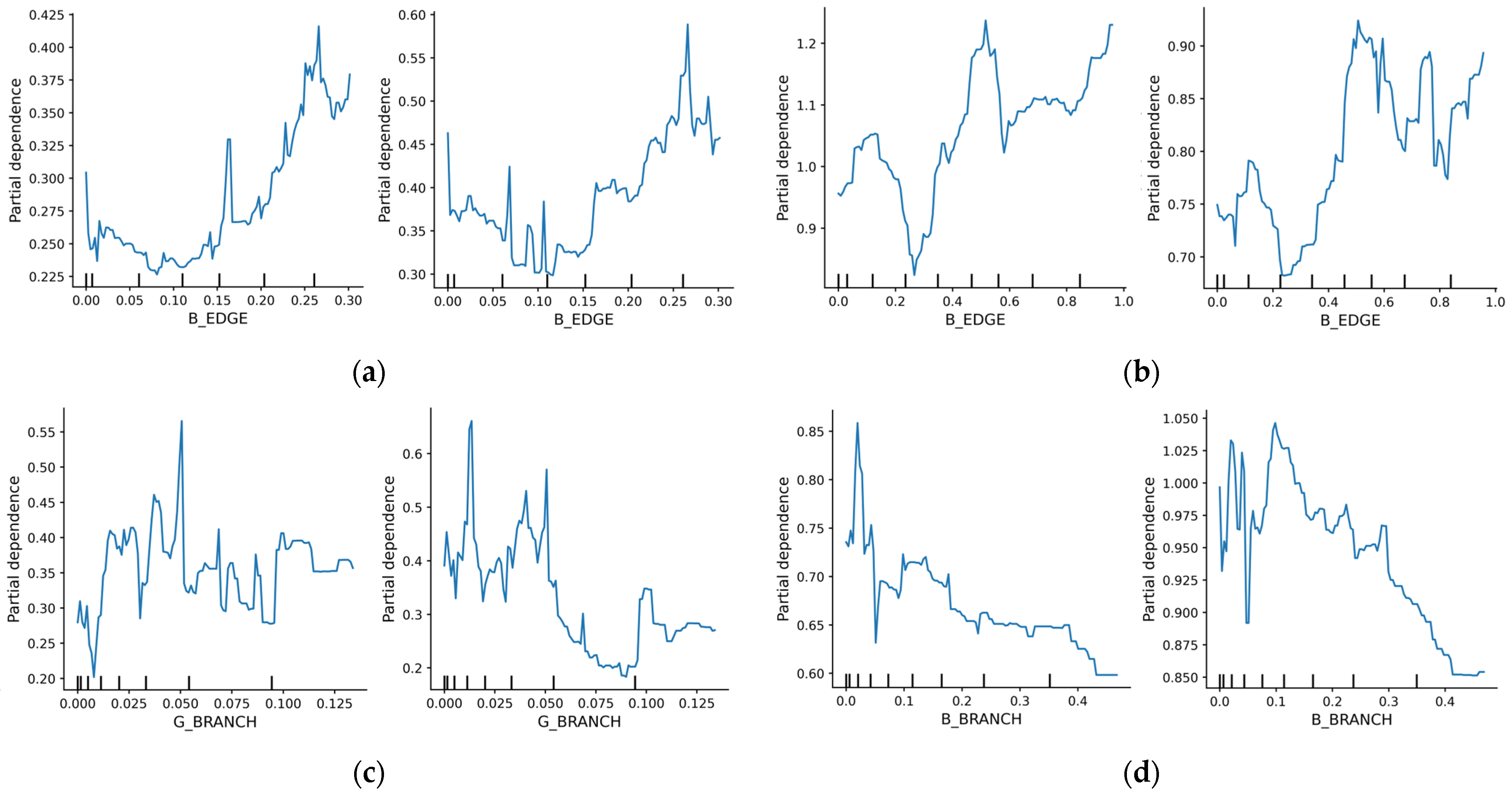
Comparative Threshold Responses of B_EDGE and G_BRANCH Indicators to the Diurnal-Night Comprehensive Crime Indicator Across Different Scales. (a) Threshold responses of the B_EDGE indicator to the diurnal-night thresholds of the comprehensive crime indicator at the 1 km scale, 2016–2020; (b) Threshold responses of the B_EDGE indicator to the diurnal-night thresholds of the comprehensive crime indicator at the 2 km scale, 2016–2020; (c) Threshold responses of the G_BRANCH indicator to the diurnal-night thresholds of the comprehensive crime indicator at the 1 km scale, 2016–2020; (d) Threshold responses of the G_BRANCH indicator to the diurnal-night thresholds of the comprehensive crime indicator at the 2 km scale, 2016–2020.
Appendix D
Table A3.
10-fold cross-validation results under 3 km grid resolution.
Appendix E
Table A4.
Global Moran’s I statistics for crime intensity across temporal phases.
Appendix F
| Algorithm A1. Integrated CatBoost–SHAP Analytical Framework |
| Input: |
| Composite gray–green indicators , log-transformed crime frequencies |
| Output: |
| Feature importance ranking, nonlinear threshold patterns, and interaction effects |
| Procedure: |
| 1. Initialize the hyperparameter search space for the CatBoost regressor. |
| 2. Perform a 10-fold cross-validation split on the 3 km grid dataset. |
| 3.: |
| -Train a CatBoost model using the RMSE objective function. |
| -Evaluate model performance on the validation fold using R2 and RMSE. |
| 4.. |
| 5. Apply the SHAP explainer to the trained CatBoost model. |
| 6. Compute SHAP values to quantify feature contributions. |
| 7. Generate SHAP dependence plots and interaction plots for gray–green variables. |
| 8. Identify nonlinear thresholds and interaction patterns. |
| Return: |
| Variable importance ranking and detected spatial threshold effects. |
References
- Lafortezza, R.; Sanesi, G. Nature-based solutions: Settling the issue of sustainable urbanization. Environ. Res. 2019, 172, 394–398. [Google Scholar] [CrossRef] [Scilit]
- Elsawy, A.A.; Ayad, H.M.; Saadallah, D. Assessing livability of residential streets—Case study: El-Attarin, Alexandria, Egypt. Alex. Eng. J. 2019, 58, 745–755. [Google Scholar] [CrossRef] [Scilit]
- Lawrence, M.; Homer-Dixon, T.; Janzwood, S.; Rockström, J.; Renn, O.; Donges, J.F. Global polycrisis: The causal mechanisms of crisis entanglement. Glob Sustain. 2024, 7, e6. [Google Scholar] [CrossRef] [Scilit]
- Charbonneau, B.; Giguère, A. The polycrisis and the uncertainty possibility space. Glob Sustain. 2025, 8, e4. [Google Scholar] [CrossRef] [Scilit]
- Oliver, T.H.; Doherty, B.; Dornelles, A.Z.; Greenwell, M.; Harrison, L.; Jones, I.; Lewis, A.; Moller, S.; Tovey, P.; Gilbert, N. Appraising cascading systemic risks, ‘watchpoints’, and interventions—Methodological reflections. Glob Sustain. 2026, 9, e4. [Google Scholar] [CrossRef] [Scilit]
- Brantingham, P.J.; Brantingham, P.L.; Andresen, M.A. The geometry of crime and crime pattern theory. J. Quant. Criminol. 2017, 33, 495–518. [Google Scholar]
- Curtis-Ham, S.; Bernasco, W.; Medvedev, O.N.; Polaschek, D. A framework for estimating crime location choice based on awareness space. Crime Sci. 2020, 9, 23. [Google Scholar] [CrossRef] [Scilit]
- Mao, Y.; Yin, L.; Zeng, M.; Ding, J.; Song, Y. Review of Empirical Studies on Relationship between Street Environment and Crime. J. Plan. Lit. 2021, 36, 187–202. [Google Scholar] [CrossRef] [Scilit]
- van Sleeuwen, S.E.M.; Ruiter, S.; Steenbeek, W. Right place, right time? Making crime pattern theory time-specific. Crime Sci. 2021, 10, 2. [Google Scholar] [CrossRef] [Scilit]
- Cadenasso, M.L.; Pickett, S.T.A.; Schwarz, K. Ecological Heterogeneity in Urban Ecosystems: Reconceptualized Land Cover Models as a Bridge to Urban Design. In Resilience in Ecology and Urban Design; Springer: Berlin/Heidelberg, Germany, 2013; Volume 3, pp. 107–127. [Google Scholar] [CrossRef] [Scilit]
- Zhou, W.; Huang, G.; Cadenasso, M.L. Does spatial configuration matter? Understanding the effects of land cover pattern on land surface temperature in urban landscapes. Landsc. Urban Plan. 2011, 102, 54–63. [Google Scholar] [CrossRef] [Scilit]
- Groff, E.R.; Lockwood, B. Criminogenic Facilities and Crime across Street Segments in Philadelphia: Uncovering Evidence about the Spatial Extent of Facility Influence. J. Res. Crime Delinq. 2014, 51, 277–314. [Google Scholar] [CrossRef] [Scilit]
- Brantingham, P.J.; Faust, F.L. A conceptual model of crime prevention. Crime Delinq. 1976, 22, 284–296. [Google Scholar] [CrossRef] [Scilit]
- Cohen, L.E.; Felson, M. Social change and crime rate trends: A routine activity approach. Am. Sociol. Rev. 1979, 44, 588–608. [Google Scholar] [CrossRef] [Scilit]
- Jacobs, J. The Death and Life of Great American Cities; Random House: New York, NY, USA, 1961. [Google Scholar]
- Newman, O. Defensible Space: People and Design in the Violent City; Architectural Press: London, UK, 1973; pp. 9–29. [Google Scholar]
- Jeffery, C.R. Crime Prevention Through Environmental Design; SAGE Publications: Thousand Oaks, CA, USA, 1997; pp. 186–206. [Google Scholar]
- Crowe, T.D. Crime Prevention Through Environmental Design; Elsevier: Oxford, UK, 2000; pp. 15–24. [Google Scholar]
- Mazzilli, C.T.S. Poetics of generative cartography. In Proceedings of the 14th Generative Art Conference (GA2011), Rome, Italy, 5–7 December 2011; pp. 495–503. [Google Scholar]
- Hanson, L.J. Cartographic Criminology: An Assessment and Proposal for an Integrated Approach to Crime Mapping. Ph.D. Thesis, University of Kent, Canterbury, UK, 2015. [Google Scholar]
- Linning, S.J.; Bowers, K.; Eck, J.E. Crime radiation theory: The co-production of crime patterns through opportunity creation and exploitation. Crime Sci. 2024, 13, 32. [Google Scholar] [CrossRef] [Scilit]
- Eck, J.E.; Linning, S.J.; Bowers, K. Does crime in places stay in places? Evidence for crime radiation from three narrative reviews. Aggress. Violent Behav. 2024, 78, 101955. [Google Scholar] [CrossRef] [Scilit]
- He, Z.; Zhang, Y.; Wang, Y.; Zhang, H.; Yao, X. Measuring the influence of multiscale geographic space on the heterogeneity of crime distribution. ISPRS Int. J. Geo-Inf. 2023, 12, 437. [Google Scholar] [CrossRef] [Scilit]
- Wang, Z.; Lu, J.; Beccarelli, P.; Yang, C. Neighbourhood permeability and burglary: A case study of a city in China. Intell. Build. Int. 2022, 14, 298–315. [Google Scholar] [CrossRef] [Scilit]
- Zeng, M.; Mao, Y.; Wang, C. The relationship between street environment and street crime: A case study of Pudong New Area, Shanghai, China. Cities 2021, 112, 103143. [Google Scholar] [CrossRef] [Scilit]
- Liu, K.; Zhang, L.; Tsou, S.; Wang, L.; Hu, Y.; Yang, K. Exploring the Complex Association Between Urban Built Environment, Sociodemographic Characteristics and Crime: Evidence from Washington, D.C. Land 2024, 13, 1886. [Google Scholar] [CrossRef] [Scilit]
- Burt, C.J.; Kondo, M.C.; Hohl, B.C.; Gong, C.H.; Bushman, G.; Wixom, C.; South, E.C.; Cunningham, R.M.; Carter, P.M.; Branas, C.C.; et al. Community Greening, Fear of Crime, and Mental Health Outcomes. Am. J. Community Psychol. 2022, 69, 46–58. [Google Scholar] [CrossRef] [Scilit] [PubMed]
- Li, B.; Li, G.; Lan, L.; Jin, A.; Lin, Z.; Wang, Y.; Chen, X. The influence mechanism of urban street environment on juvenile delinquency based on multi-source data fusion: A case study of Manhattan, New York. Comput. Urban Sci. 2024, 4, 26. [Google Scholar] [CrossRef] [Scilit]
- Mansourihanis, O.; Maghsoodi Tilaki, M.J.; Sheikhfarshi, S.; Mohseni, F.; Seyedebrahimi, E. Addressing Urban Management Challenges for Sustainable Development: Analyzing the Impact of Neighborhood Deprivation on Crime Distribution in Chicago. Societies 2024, 14, 139. [Google Scholar] [CrossRef] [Scilit]
- Dear, K.; Dutton, K.; Fox, E. Do ‘watching eyes’ influence antisocial behavior? A systematic review and meta-analysis. Evol. Hum. Behav. 2019, 40, 269–280. [Google Scholar] [CrossRef] [Scilit]
- Ceccato, V.; Gaudelet, N.; Graf, G. Crime and safety in transit environments: A systematic review of the English and the French literature, 1970–2020. Public Transp. 2022, 14, 105–153. [Google Scholar] [CrossRef] [Scilit]
- Ventorim, F.C.; Netto, V.M. The Hidden Connections of Urban Crime: A Network Analysis of Victims, Crime Types, and Locations in Rio de Janeiro. Urban Sci. 2024, 8, 72. [Google Scholar] [CrossRef] [Scilit]
- Roy, S. Visibility matters: Constructing safe passages on the streets of Kolkata. J. Urban Aff. 2024, 46, 1433–1451. [Google Scholar] [CrossRef] [Scilit]
- International CPTED Association. ICA Newsletters. Available online: https://www.cpted.net/ICA-newsletters (accessed on 15 January 2025).
- Fujii, T.; Fujikawa, Y.; Oikawa, K. A quantitative analysis of natural surveillance at elementary schools. J. Asian Archit. Build. Eng. 2013, 12, 17–23. [Google Scholar] [CrossRef] [Scilit]
- Jing, F.; Liu, L.; Zhou, S.; Song, J.; Wang, L.; Zhou, H.; Wang, Y.; Ma, R. Assessing the Impact of Street-View Greenery on Fear of Neighborhood Crime in Guangzhou, China. Int. J. Environ. Res. Public Health 2021, 18, 311. [Google Scholar] [CrossRef] [Scilit]
- Oh, H.-N.; Kang, S.-J. A study on crime characteristics and CPTED application of neighborhood walking trails. J. Archit. Inst. Korea 2025, 41, 103–112. [Google Scholar]
- Gu, H.; Sui, J.; Chen, P. Graph Representation Learning for Street-Level Crime Prediction. ISPRS Int. J. Geo-Inf. 2024, 13, 229. [Google Scholar] [CrossRef] [Scilit]
- Mao, Y.; Dai, S.; Ding, J.; Zhu, W.; Wang, C.; Ye, X. Space–Time Analysis of Vehicle Theft Patterns in Shanghai, China. ISPRS Int. J. Geo-Inf. 2018, 7, 357. [Google Scholar] [CrossRef] [Scilit]
- Cheng, W.; Rao, Y.; Tang, Y.; Yang, J.; Chen, Y.; Peng, L.; Hao, J. Identifying the Spatio-Temporal Characteristics of Crime in Liangshan Prefecture, China. Int. J. Environ. Res. Public Health 2022, 19, 10862. [Google Scholar] [CrossRef] [Scilit]
- Zhang, H.; Gao, Y.; Yao, D.; Zhang, J. Interaction of Crime Risk across Crime Types in Hotspot Areas. ISPRS Int. J. Geo-Inf. 2023, 12, 176. [Google Scholar] [CrossRef] [Scilit]
- Clutter, J.E.; Peterson, S.; Henderson, S.; Haberman, C.P. Understanding the impact of weather and potentially criminogenic places on street robbery. Crime Sci. 2024, 13, 42. [Google Scholar] [CrossRef] [Scilit]
- Jonescu, E.E.; Ramanayaka, C.E.; Olatunji, O.A.; Uylaki, T.J. Understanding the impact of urban heat islands on crime: Insights from temperature, population density, and green canopy cover. Crime Sci. 2024, 13, 15. [Google Scholar] [CrossRef] [Scilit]
- Zou, Y.; Chen, J.; Zong, H. Is shading a better way to cool down? Evaluation and comparison of the cooling capacity of blue-green spaces and urban shade. Ecol. Indic. 2024, 167, 112688. [Google Scholar] [CrossRef] [Scilit]
- Cozens, P.; Love, T.; Davern, B. Geographical Juxtaposition: A New Direction in CPTED. Soc. Sci. 2019, 8, 252. [Google Scholar] [CrossRef] [Scilit]
- Kim, G.; Cho, Y.; Han, Y.; Lee, G. Crime mapping in urban environments using explainable AI: A case study of Daegu, Korea. Sustain. Cities Soc. 2025, 130, 106507. [Google Scholar] [CrossRef] [Scilit]
- Sampson, R.J.; Groves, W.B. Community structure and crime: Testing social-disorganization theory. Am. J. Sociol. 1989, 94, 774–802. [Google Scholar] [CrossRef] [Scilit]
- Guerette, R.T.; Bowers, K. Assessing the extent of crime displacement and diffusion of benefits. Criminology 2009, 47, 1331–1368. [Google Scholar] [CrossRef] [Scilit]
- Han, Z.; Xie, W.; Jiang, R.; Huang, Q.; Chen, T.; Chen, R. Relationship between the street spatial environment and crime based on quantitative network analysis. Proc. ACM Hum.-Comput. Interact. 2024, 8, 3708230. [Google Scholar]
- Awaryi Churchill, S.; Hayward, M.; Smyth, R.; Trinh, T. Crime, community social capital and entrepreneurship. J. Bus. Ventur. 2023, 38, 106291. [Google Scholar] [CrossRef] [Scilit]
- Andresen, M.A.; Frank, R.; Felson, M. Age and the distance to crime. Criminol. Crim. Justice 2013, 14, 314–333. [Google Scholar] [CrossRef] [Scilit]
- Weisburd, D.; Zastrow, T.; Kuen, K.; Andresen, M.A. Crime concentrations at micro places: A review of the evidence. Aggress. Violent Behav. 2024, 78, 101979. [Google Scholar] [CrossRef] [Scilit]
- Troy, A.; Morgan Grove, J.; O’Neil-Dunne, J. The relationship between tree canopy and crime rates across an urban–rural gradient in the greater Baltimore region. Landsc. Urban Plan. 2012, 106, 262–270. [Google Scholar] [CrossRef] [Scilit]
- Othman, F.; Mohd Yusoff, Z.; Abdul Rasam, A.R. Isovist and visibility graph analysis (VGA): Strategies to evaluate visibility along movement pattern for safe space. IOP Conf. Ser. Earth Environ. Sci. 2019, 385, 012024. [Google Scholar] [CrossRef] [Scilit]
- Chen, Y.; Li, Y.; Li, J. Investigating the Influence of Tree Coverage on Property Crime: A Case Study in the City of Vancouver, British Columbia, Canada. ISPRS Int. Arch. Photogramm. Remote Sens. Spatial Inf. Sci. 2016, XLI-B2, 695–702. [Google Scholar] [CrossRef] [Scilit]
- Venter, Z.S.; Shackleton, C.; Faull, A.; Lancaster, L.; Breetzke, G.; Edelstein, I. Is green space associated with reduced crime? A national-scale study from the Global South. Sci. Total Environ. 2022, 825, 154005. [Google Scholar] [CrossRef] [Scilit]
- Schertz, K.E.; Saxon, J.; Cardenas-Iniguez, C.; Bettencourt, L.M.A.; Ding, Y.; Hoffmann, H.; Berman, M.G. Neighborhood street activity and greenspace usage uniquely contribute to predicting crime. npj Urban Sustain. 2021, 1, 19. [Google Scholar] [CrossRef] [Scilit]
- Wang, X.; Zhou, L.; López-Carr, D.; Song, Y.; Gao, H.; Che, T.; Liu, Z.; Wei, W. Urban grey-green scales: A new perspective for assessing dynamic spatial trade-offs. Int. J. Appl. Earth Obs. Geoinf. 2025, 142, 104808. [Google Scholar] [CrossRef] [Scilit]
- Caplan, J.M.; Kennedy, L.W.; Piza, E.L. Environmental crime enforcement: Assessing the impact of police activity on violations. J. Environ. Manag. 2013, 128, 843–851. [Google Scholar]
- Caplan, J.M.; Piza, E.L.; Kennedy, L.W. Citizen reporting of environmental crime. Crime Prev. Community Saf. 2013, 15, 187–205. [Google Scholar]
- Anyinam, K. Transnational environmental crime in Africa: Challenges and opportunities for regional cooperation. J. Environ. Law Policy 2015, 24, 163–188. [Google Scholar]
- Zhang, Y.; Kwan, M.-P.; Fang, L. An LLM driven dataset on the spatiotemporal distributions of street and neighborhood crime in China. Sci. Data 2025, 12, 467. [Google Scholar] [CrossRef] [Scilit] [PubMed]
- Chen, Z.; Yu, B.; Yang, C.; Zhou, Y.; Yao, S.; Yao, S.; Qian, X.; Wang, C.; Wu, B.; Wu, J. An Extended Time Series (2000–2018) of Global NPP-VIIRS-Like Nighttime Light Data from a Cross-Sensor Calibration. Remote Sens. 2021, 13, 889. [Google Scholar] [CrossRef] [Scilit]
- Soille, P.; Vogt, P. Morphological segmentation of binary patterns. Pattern Recognit. Lett. 2009, 30, 456–459. [Google Scholar] [CrossRef] [Scilit]
- Vogt, P.; Larondelle, N.; Giordano, B. Morphological spatial pattern analysis (MSPA) for detecting forest cover patterns in raster maps. Landsc. Ecol. 2007, 23, 1107–1117. [Google Scholar]
- Li, H.; Wu, J. Use and misuse of landscape indices. Landsc. Ecol. 2004, 19, 389–399. [Google Scholar] [CrossRef] [Scilit]
- McGarigal, K.; Cushman, S.A.; Ene, E. FRAGSTATS v4: Spatial Pattern Analysis Program for Categorical and Continuous Maps; University of Massachusetts: Amherst, MA, USA, 2012. [Google Scholar]
- Dormann, C.F.; Elith, J.; Bacher, S.; Buchmann, C.; Carl, G.; Carré, G.C.G.; Márquez, J.R.G.; Gruber, B.; Lafourcade, B.; Leitao, P.J.; et al. Collinearity: A review of methods to deal with it and a simulation study evaluating their performance. Ecography 2013, 36, 27–46. [Google Scholar] [CrossRef] [Scilit]
- Lundberg, S.M.; Lee, S.-I. A unified approach to interpreting model predictions. In Proceedings of the 31st International Conference on Neural Information Processing Systems, Long Beach, CA, USA, 4–9 December 2017; pp. 4768–4777. [Google Scholar]
- Hoang, N.D. Machine learning approaches for geospatial modeling of urban land surface temperature. Sensors 2025, 25, 5380. [Google Scholar] [CrossRef] [Scilit]
- Liu, Q.; Hang, T.; Wu, Y. Unveiling differential impacts of multidimensional urban morphology on heat island effect across local climate zones. Build. Environ. 2025, 270, 112574. [Google Scholar] [CrossRef] [Scilit]
- Saraiva, M.; Teixeira, B. Exploring the spatial relationship between street crime events and the distribution of urban greenspace: The case of Porto, Portugal. ISPRS Int. J. Geo-Inf. 2023, 12, 492. [Google Scholar] [CrossRef] [Scilit]
- Li, D.; Han, H.Z.; Wang, J.; Xiao, X. Explaining Urban Vitality Through Interpretable Machine Learning: A Big Data Approach Using Street View Images and Environmental Factors. Sustainability 2025, 17, 4962. [Google Scholar] [CrossRef] [Scilit]
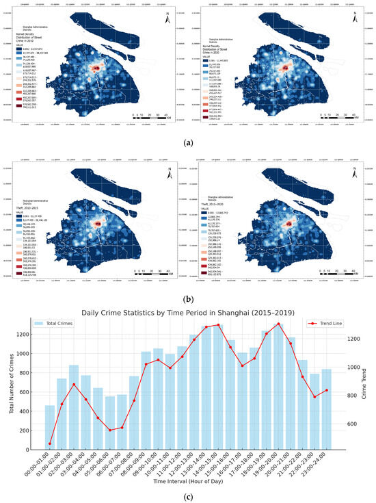
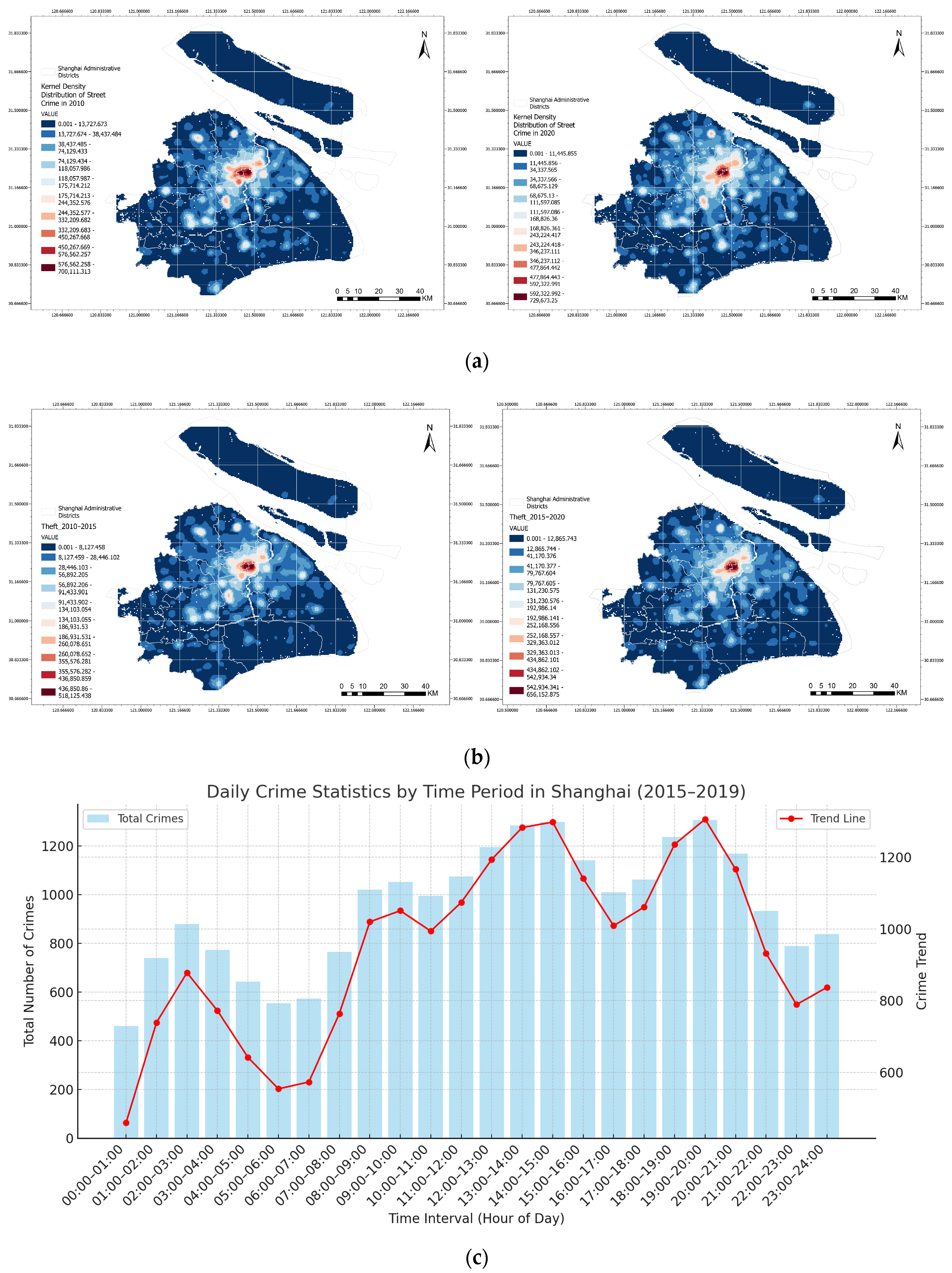
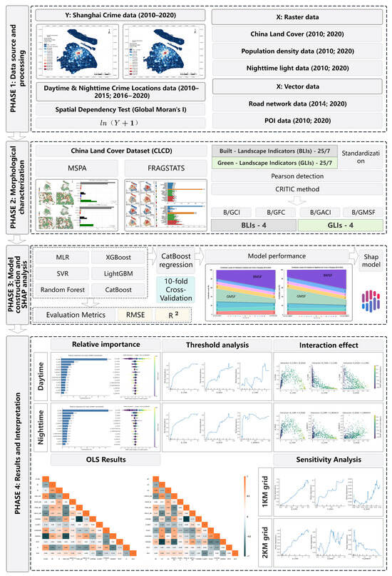
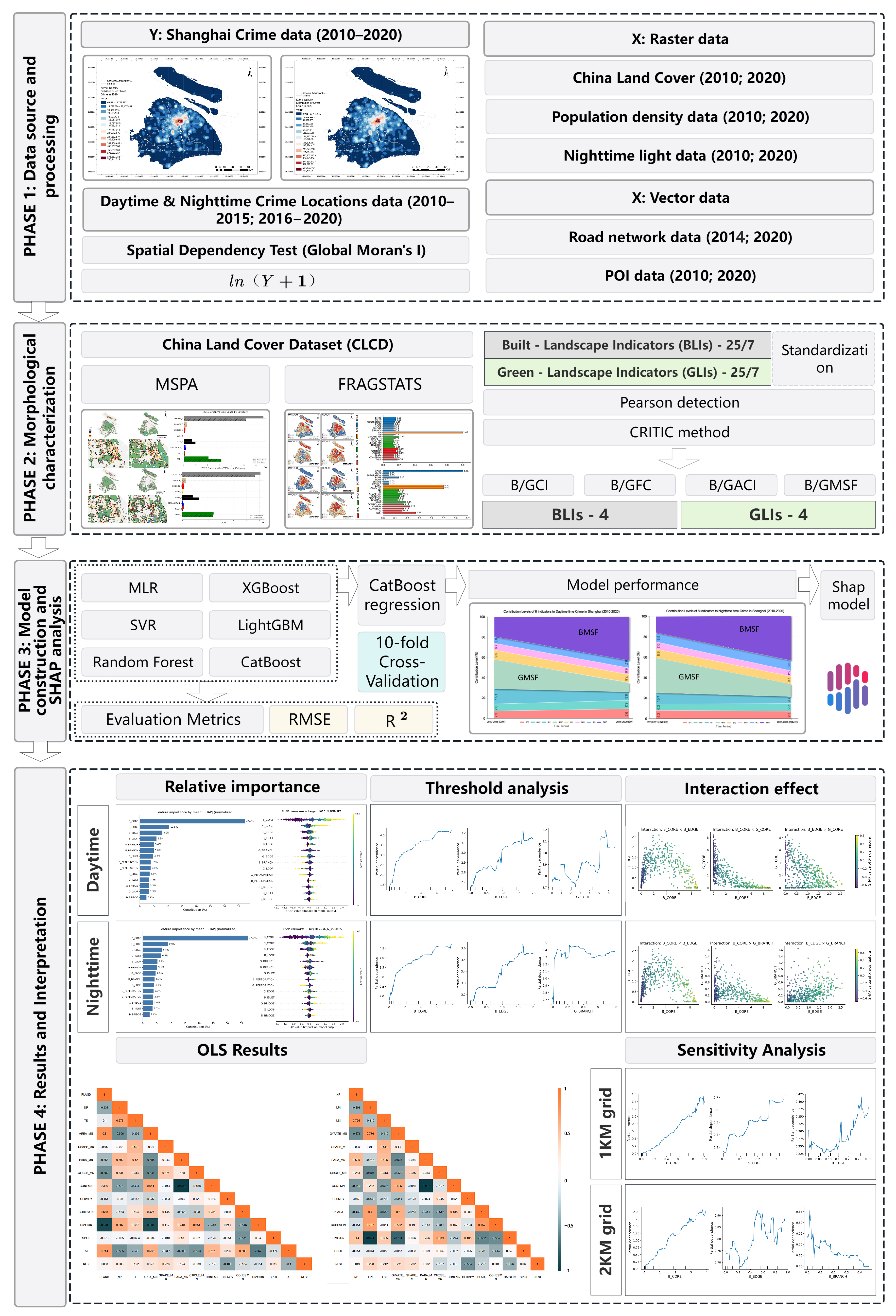
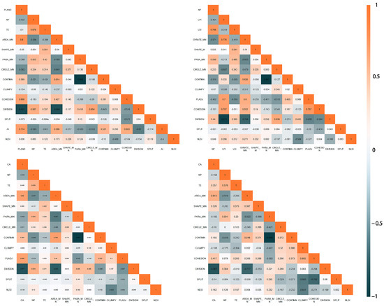
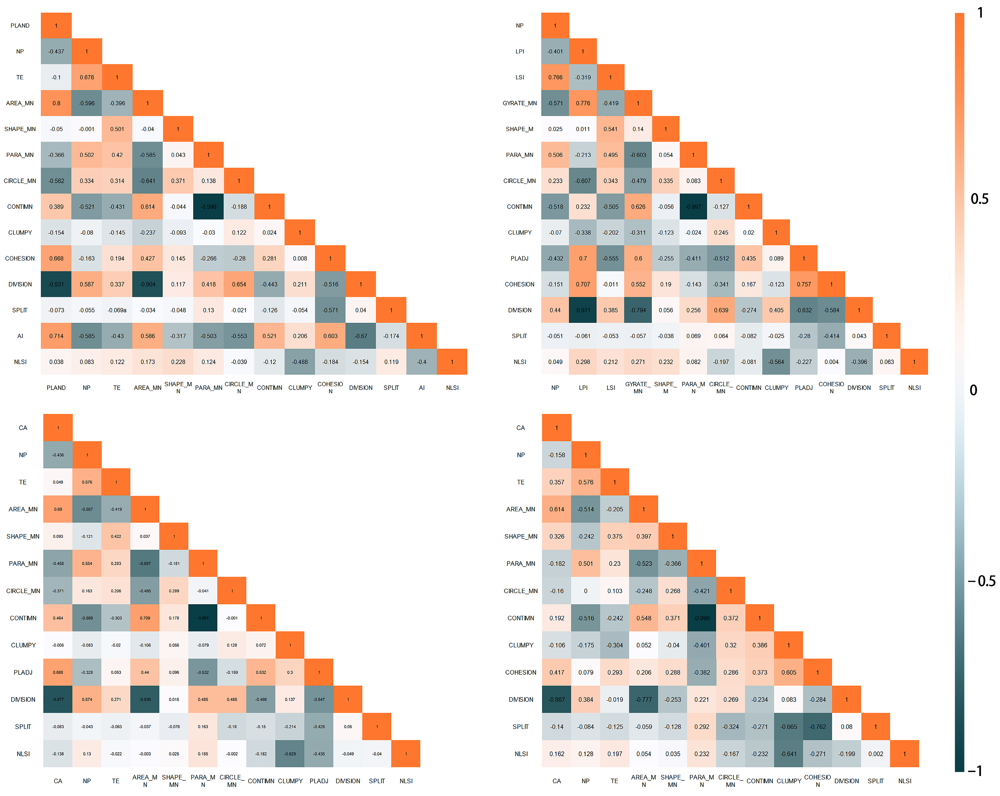
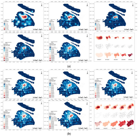
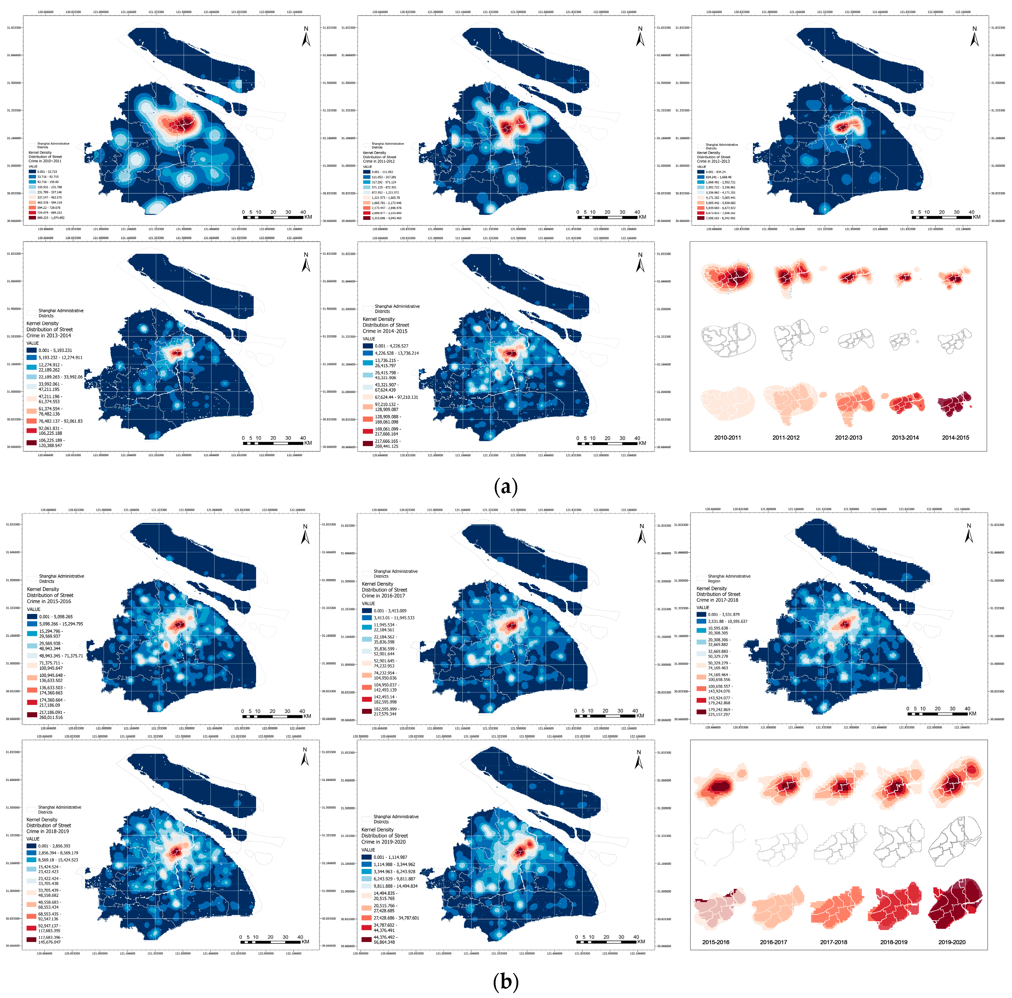
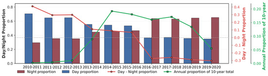
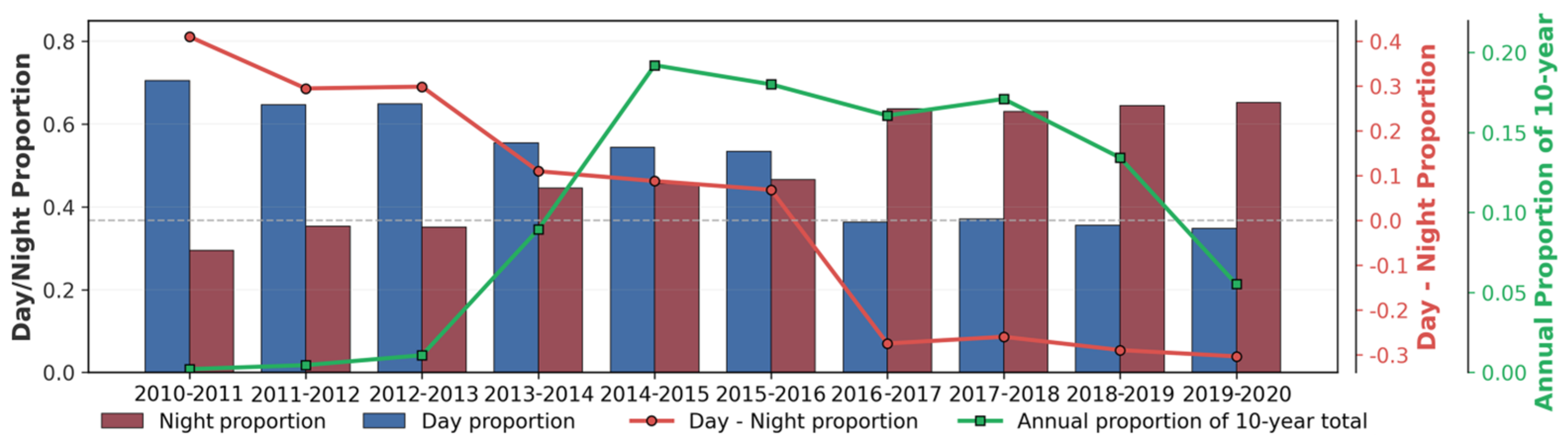
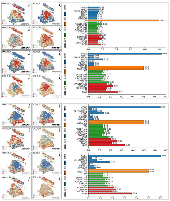
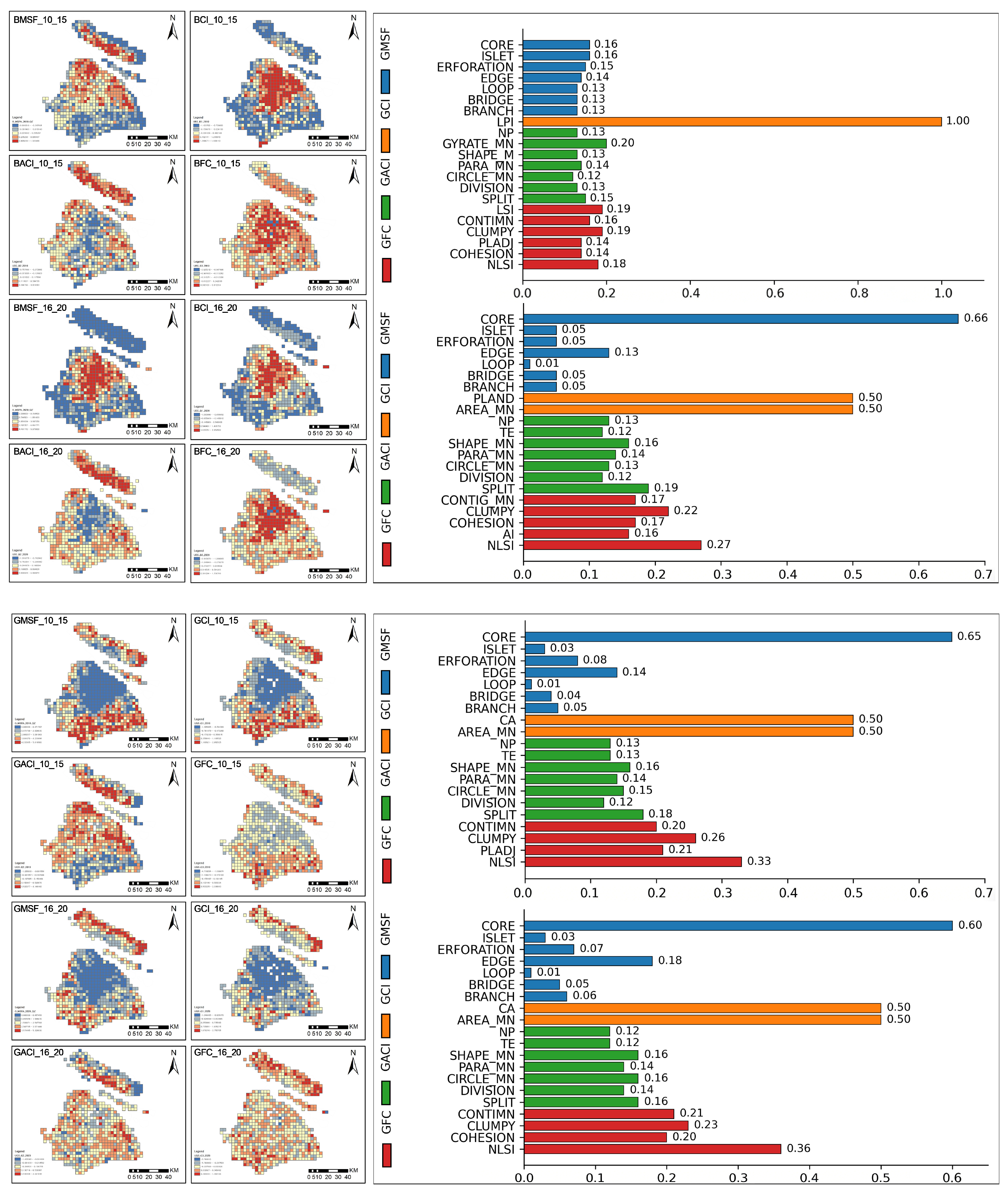
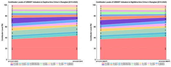
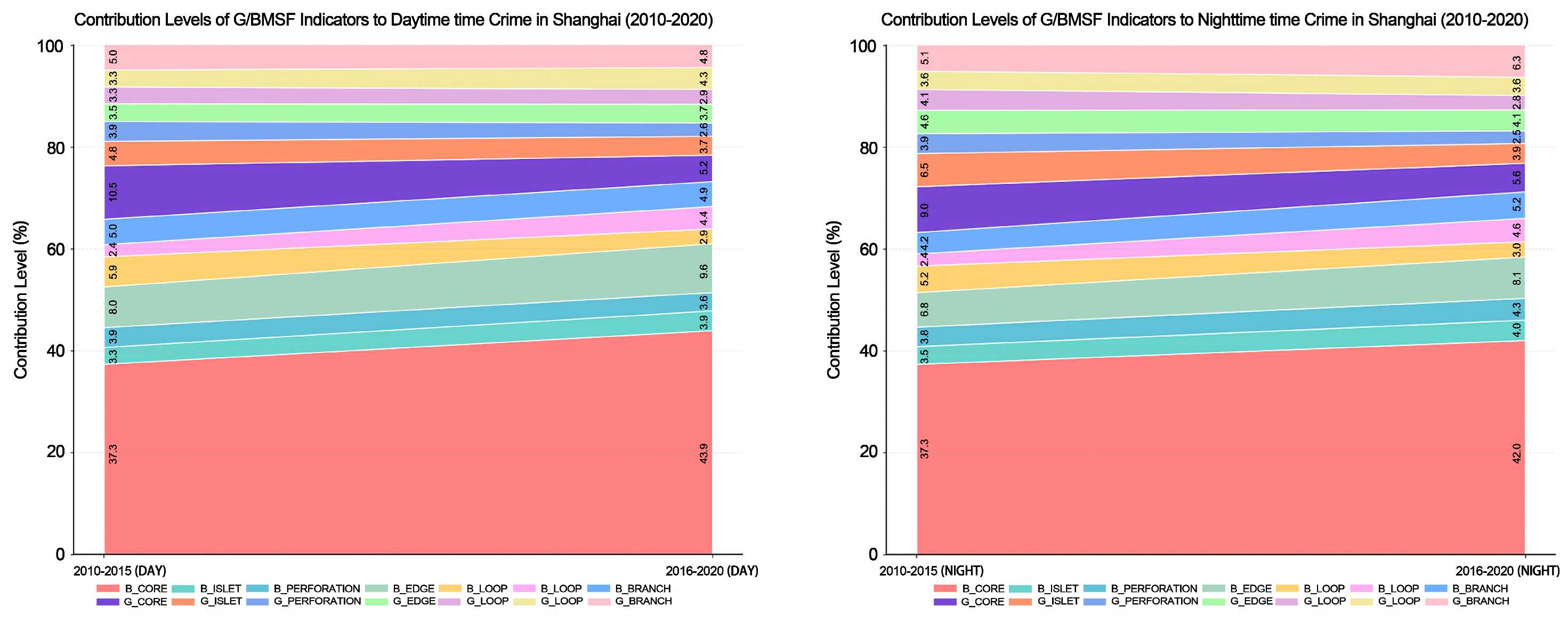
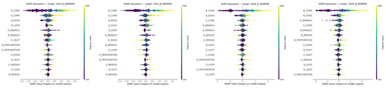
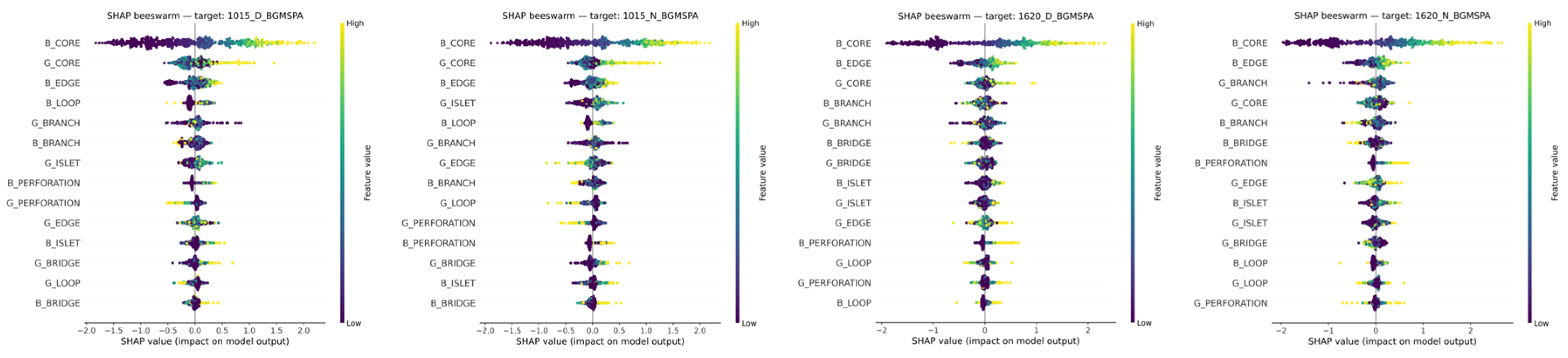
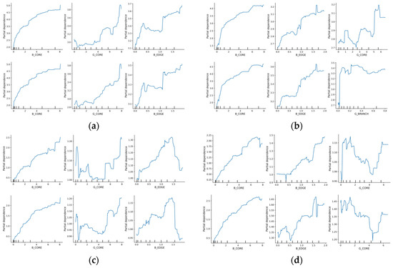
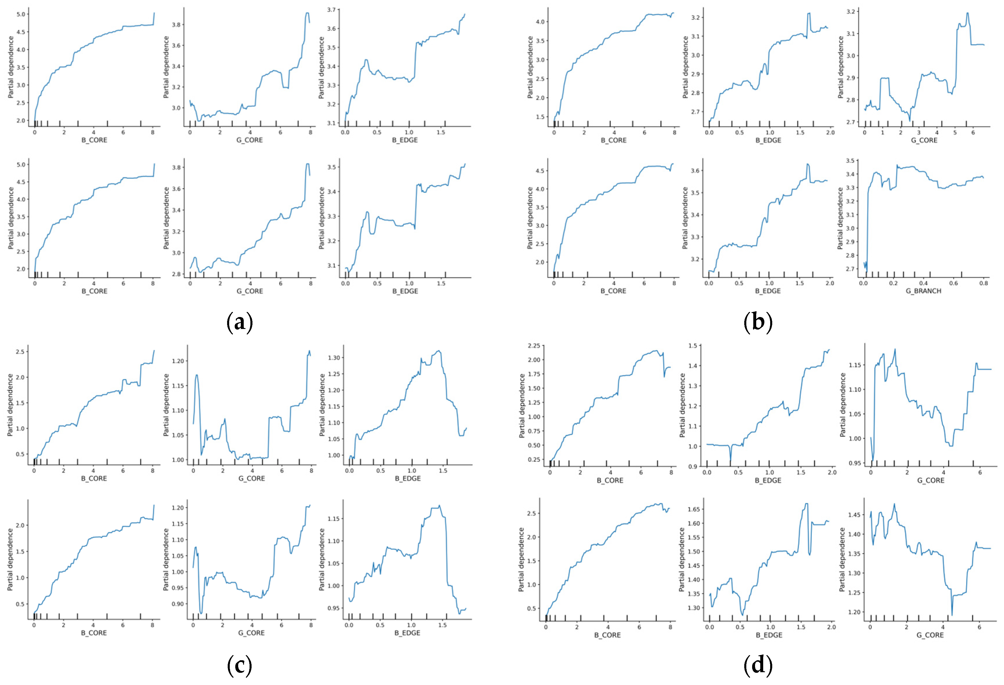
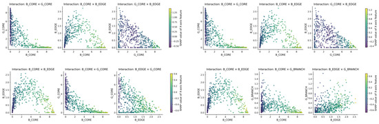
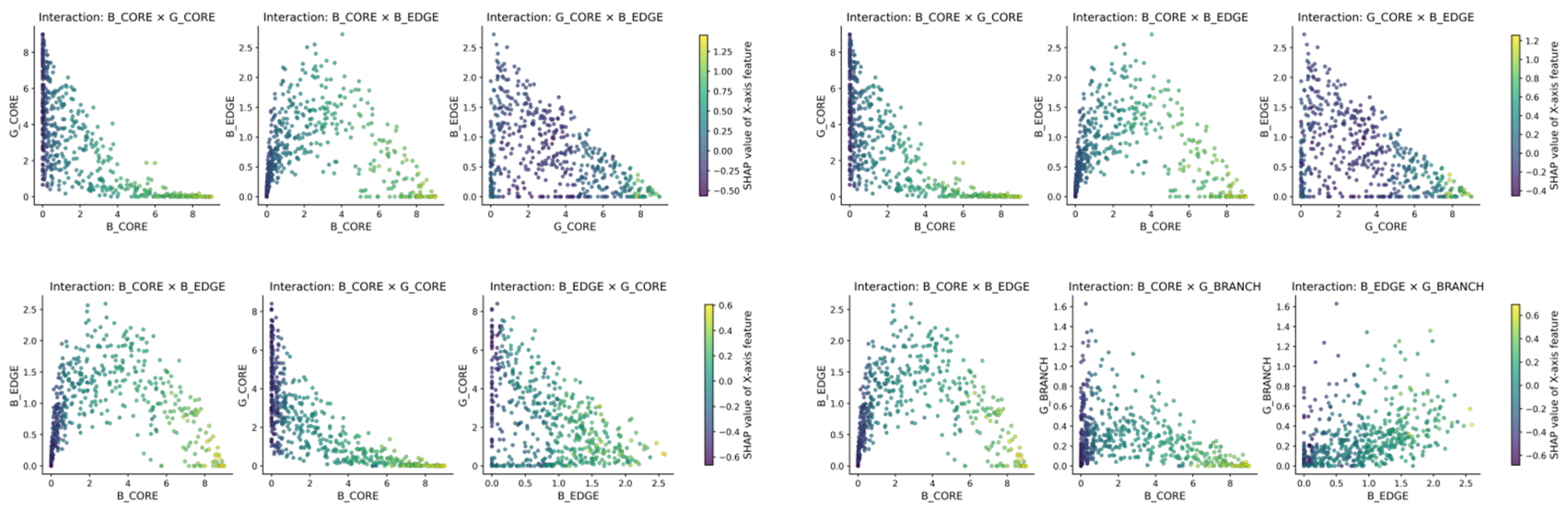

Disclaimer/Publisher’s Note: The statements, opinions and data contained in all publications are solely those of the individual author(s) and contributor(s) and not of MDPI and/or the editor(s). MDPI and/or the editor(s) disclaim responsibility for any injury to people or property resulting from any ideas, methods, instructions or products referred to in the content. |
© 2026 by the authors. Published by MDPI on behalf of the International Society for Photogrammetry and Remote Sensing. Licensee MDPI, Basel, Switzerland. This article is an open access article distributed under the terms and conditions of the Creative Commons Attribution (CC BY) license.