


Abstract
While parameters such as slope and aspect are routinely considered in solar radiation modelling, the role of terrain or surface roughness remains underexplored, with no universally accepted method for its calculation. This study compares several approaches to quantifying terrain or surface roughness in several geographical information system (GIS) environments (ArcGIS, QGIS, WhiteboxTools, and SAGA GIS) and introduces local fractal dimension, computed using a custom Python script, as an additional metric. The aim is to evaluate the influence of surface roughness on potential solar radiation modelling and to examine its relationship with other terrain parameters. The analysis is based on case studies from both a rugged alpine environment in the Tatra Mountains (Tichá and Kôprová dolina (valleys), Kriváň peak; 944–2467 m a.s.l.) and an urban environment (the city of Poprad, near the High Tatras, Slovakia). The results demonstrate that surface roughness can significantly affect potential solar radiation modelling in areas with high surface variability. The findings are applicable not only to solar radiation studies, but also to other fields of spatial modelling, where incorporating surface roughness can improve the accuracy and robustness of spatial analyses and predictions.
1. Introduction
The influence of terrain or surface roughness on phenomena such as solar illumination is well established [1,2,3]. Elevated areas naturally cast shadows on lower-lying regions. This shading is caused by terrain ruggedness, vegetation [4,5], and, in urban areas, by buildings and other structures [6]. The question, however, is how to calculate surface roughness, quantify its influence, or incorporate it into spatial analyses.
The calculation of terrain or surface roughness is not straightforward. Several methods have been proposed and applied [7,8,9,10,11,12,13,14], most of which are based on deviations in elevation or variations in slope angles. All methods depend on the selected neighbourhood for the calculation and the resolution of the input raster. These include measures such as raster roughness (RR) [7], the Topographic Ruggedness Index (TRI) [8], the Multiscale Roughness (MSR) [12,13], and the local fractal dimension (LFD) [15]. Although fractal dimension (FD) is a lesser-known parameter, its significance in studying the Earth’s surface is supported by numerous studies that have shown that topography, particularly mountainous regions, exhibits fractal behaviour [16,17,18]. Rather than exact self-similarity, both continental topography and seafloor bathymetry are generally self-affine and statistically self-similar over finite ranges of scale, and the apparent smoothness reflects limited scaling at a given resolution [19,20,21]. The FD thus also serves as a quantitative indicator of surface roughness.
Despite the availability of multiple surface roughness metrics, their role in solar radiation modelling remains unclear. In particular, the relationship between roughness measures and the accuracy of potential solar radiation (PSR) estimates has not been sufficiently investigated, including for fractal-based metrics such as LFD.
The aim of this paper is therefore to address this gap by systematically evaluating the relationship between surface roughness metrics and the reliability of potential solar radiation modelling, with particular emphasis on fractal-based approaches such as LFD.
In spatial analyses and geographical information systems (GISs), fractals have been applied in various ways, ranging from calculating soil roughness using Synthetic Aperture Radar (SAR) data [22], modelling forest dynamics [23], terrain restoration [24], assessing territorial road networks [25], examining urban land-cover spatial patterns [26], and studying the planar spatial morphology of mountain settlements [27]. Furthermore, Aguado et al. [28] employed multifractal analysis of digital elevation model (DEM) data for the spatial characterisation of landscapes, while Chen [29] applied FD calculations to the description of urban morphology, addressing concepts such as the “fractal city” introduced by Batty and Longley [30]. Urban FD calculation is further discussed in [31]. Moreover, fractal analysis has also been applied to DEMs derived from LiDAR data [32,33], similar to our work. Fractals have also been used in modelling solar radiation and its uncertainties [33,34,35,36]. Among the few recent studies linking solar radiation modelling with FD calculations in GIS, Tara et al. [33] stands out, though it primarily focuses on urban environments. In this paper, we focus on modelling surface roughness also in high-mountain environments for the purposes of GIS-based solar radiation modelling, especially in vegetated mountainous areas.
The calculation of potential solar radiation (PSR) is both time- and computation-intensive. Therefore, according to Ďuračiová and Pružinec [37] and Buchalová et al. [5], a potential solution is to identify areas requiring precise modelling due to complex 3D structures and vegetation, while, in other areas, approximate estimation based on lower-resolution DEMs may suffice. Note that the spatial resolution of elevation models significantly affects the representation of terrain morphology and derived surface parameters. In LiDAR-derived datasets, this is closely linked to point cloud density, which influences the geometric accuracy of surface representation and, consequently, applications such as solar radiation modelling [38,39].
The accuracy of PSR estimates in high-mountain environments related to terrain parameters is also addressed in [37]. It highlights that the primary spatial distribution factor of PSR and the accuracy of its determination is geo-relief, particularly elevation and its derived parameters (e.g., topographic position index (TPI)). We hypothesise that the roughness of the relief could also be a suitable parameter for identifying complex 3D structures as risk sites for the accurate calculation of PSR. The relationship between relief roughness and solar radiation has been addressed, for example, in works [40,41]. Recent research also indicates that topographic shadowing and surface morphology significantly influence the accuracy of solar radiation [42].
In this article, we therefore investigate the impact of surface roughness on the accuracy of GIS-based solar radiation calculation both in rugged mountainous areas and in urban environments. The analysis involves calculating PSR and terrain parameters, including roughness, using various GIS software environments (ArcGIS Pro 3.1.0, QGIS 3.40 Bratislava and WhiteboxTools, and SAGA GIS 9.8.1), as well as custom-developed tools. As a case study, we first conducted PSR calculation in the rugged high-mountain environment of the High Tatra Mountains, specifically in the area of the Tichá dolina and Kôprová dolina, two valleys near Kriváň (peak, elevation 2495 m) (Figure 1). One of our goals is to contribute to more reliable GIS-based PSR modelling, particularly in mountainous areas where solar radiation strongly influences geological and ecological processes [43]. The second case study is carried out in the city of Poprad (near the High Tatras, Slovakia) (Figure 2), with the aim of showing surface roughness calculation and its impact on PSR even in urban environments. Moreover, given the potential use of terrain or surface roughness as a parameter in various types of spatial predictive modelling, we consider it important to know its dependence on other commonly used relief parameters—this is also one of the partial goals of the article.
Figure 1.
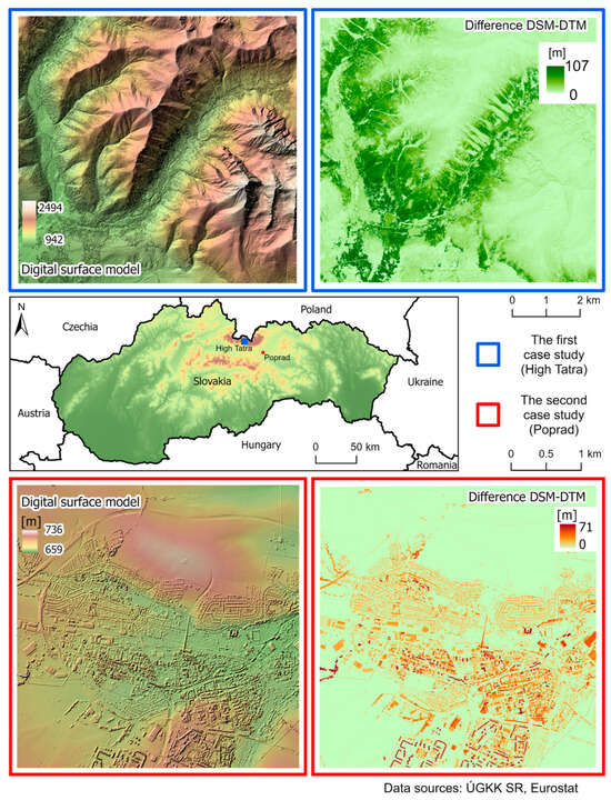
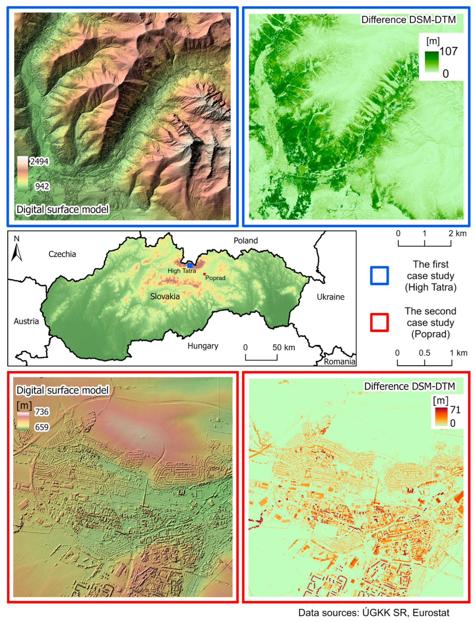
Case study areas—blue outlines indicate maps related to the first case study (Tatras), while red outlines indicate those related to the second case study (Poprad). Top left: orthophoto map; top right: digital surface model (DSM); bottom left: difference between DSM and DTM; bottom right: area of the second case study (Poprad). (Data sources: DTM 5.0 and DSM 1.0 provided by GCCA SR/ÚGKK SR [44]; state boundaries provided by Eurostat).
Figure 2.
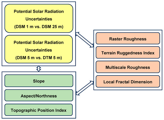
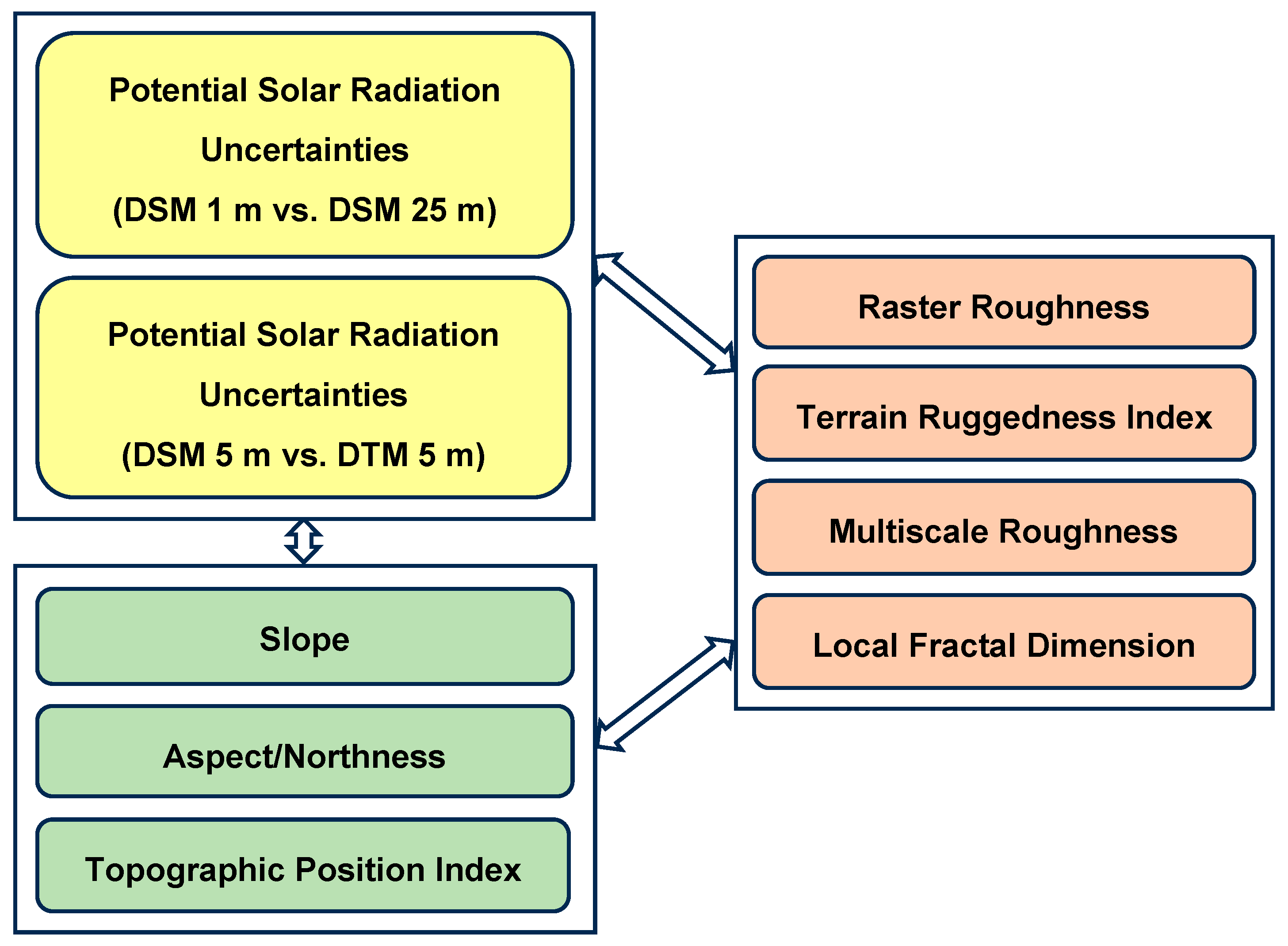
Analysis scheme. Arrows indicate the calculation of pairwise Pearson correlations between raster outputs, including correlations among parameters within each parameter group (rectangles). Abbreviations: DSM—digital surface model; DTM—digital terrain model.
The partial aims of this paper are therefore fourfold: (1) to examine the current availability of tools for surface roughness calculation in GIS environments; (2) to introduce LFD as a surface roughness metric; (3) to assess the independence of roughness parameters from other terrain parameters; and (4) to evaluate the influence of surface roughness on PSR modelling.
This article is structured as follows: Section 2 describes the case studies, the experimental design and the methodology for calculating terrain and roughness parameters, including LFD, concerning the software tools used. Section 3 details the analysis results, while the final sections offer their interpretation, discussion, and recommendations.
2. Materials and Methods
First, Section 2.1 presents case studies illustrating the issue addressed and indicating the practical application of the proposed approach. The following sections detail each stage of the workflow: design of the experiment (Section 2.2), calculation of individual terrain parameters and surface roughness (Section 2.3, Section 2.4 and Section 2.5), PSR estimation (Section 2.6), and statistical analysis of mutual correlations (Section 2.7). Section 2.8 explains the approach used for reclassifying and clustering the resulting values.
2.1. Case Studies and Data Used
The first case study was conducted within a selected area of 8 × 8 km located in the Kôprová and Tichá dolina (valleys below Kriváň peak, Vysoké Tatry/High Tatras, elevations in the range of 944 m to 2495 m, Figure 1). This area was chosen due to its highly variable terrain, encompassing high mountain peaks and ridges, valleys, and water bodies. Another reason was that it includes areas both with and without dense vegetation, particularly tree cover. The second case study area is located in the urbanised area of the city of Poprad, near the High Tatras (4 × 4 km, Figure 1).
Within these areas, we calculated the terrain parameters, roughness parameters, and PSR based on the digital terrain model (DTM) and digital surface model (DSM) at spatial resolutions of 1 m, 5 m, and 25 m. To assess the impact on the accuracy of PSR estimation, we also calculated the absolute differences between the PSR models derived using different resolutions (1 m vs. 25 m) and data sources (DTM vs. DSM).
The DTM (version 5.0) and DSM (version 1.0) covering the entire territory of Slovakia [44] are provided by the Geodesy, Cartography and Cadastre Authority of the Slovak Republic (GCCA SR; in Bratislava, Slovak, ÚGKK SR). LiDAR data for the Tatra Mountains were acquired by airborne laser scanning (ALS) within the national project of the GCCA SR using an RIEGL VQ-780i airborne laser scanner [45]. The dataset originates from LOT 26 (Tatry), where LOT refers to a contractual acquisition unit used to divide the nationwide LiDAR survey into several territorial blocks [45]. In the Tatra region (the area of our case study, LOT26—Tatry), the average density of points of the last reflection is up to 30 points per m2, the vertical accuracy of the point cloud and DTM in ETRS89-h is 0.04 m, and the horizontal accuracy of the point cloud in ETRS89-TM-34 is 0.1 m [44]. Both DTM and DSM derived from ALS are also available in raster format with a spatial resolution of 1 m. The data are freely available; however, users are required to cite the source in any derived work or publication as follows: “ÚGKK SR”. For this case study, we used the DTM 5.0 (for terrain parameters and PSR calculation) and DSM 1.0 (for roughness parameters and PSR calculation) at a spatial resolution of 1 m, in the national reference coordinate system S-JTSK[JTSK03] (EPSG 8353). These rasters were subsequently aggregated to resolutions of 5 m and 25 m for further analysis.
2.2. Design of the Experiment
Based on the objectives of this study, we designed a workflow to compare the effects of multiple roughness metrics on PSR outputs derived from both DSM and DTM data, and to examine whether the roughness parameters are independent of other terrain parameters. The results were compared both visually and quantitatively using Pearson’s correlation coefficients calculated between raster outputs. Spatial autocorrelation was assessed using Moran’s I for each variable. Because spatial dependence violates the assumptions of classical correlation analysis, the statistical significance of the observed relationships was further evaluated using a permutation-based approach, providing more robust inference.
We hypothesised that the uncertainties in PSR calculation were correlated not only with the absolute values of TPI [37], but also with surface roughness. A further aspect considered in this study was the extent to which these parameters influence uncertainties arising from reduced resolution or from the substitution of DSM with DTM data (e.g., in cases where current DSM data are not available).
The experimental design for this study is illustrated schematically in Figure 2.
We computed correlation coefficients between individual parameters (5 m resolution) to quantify their relationships. The objective was to understand dependencies among these parameters, particularly regarding their potential use in predictive spatial modelling, and to evaluate their correlations with uncertainties in PSR calculations. In this study, the tested uncertainties arise from differences between DTM and DSM data, as well as from the use of reduced spatial resolutions (1 m, 5 m, and 25 m). Uncertainties were quantified as absolute differences.
2.3. Calculation of Basic Elevation-Derived Terrain Parameters
Key commonly used terrain parameters, including slope, aspect, and the TPI, were calculated from high-resolution DTM data (1 m raster resolution). These parameters are essential for characterising the spatial variability of the terrain and its influence on solar radiation distribution.
2.3.1. Slope, Aspect, and Northness
Slope and aspect are fundamental terrain parameters frequently used in spatial modelling and the prediction of spatial phenomena. We calculated these parameters using ArcGIS Pro 3.1.0 software, although the same algorithms are implemented in, e.g., QGIS. The calculation is based on the differences between the raster cell value and the values of its neighbouring cells [46,47].
Although aspect is an important terrain parameter, it is not easy to include it directly in the analysis due to its circular nature (0° to 360°, where 0° and 360° represent the same direction). For this reason, we transform it into the northness parameter for further correlation analysis [37]:
This parameter ranges from −1 (south-facing slopes) to 1 (north-facing slopes).
2.3.2. Topographic Position Index
The topographic position index (TPI) [48] is a valuable terrain parameter with a straightforward calculation:
where represents the elevation of the raster cell, and is the mean elevation of its surrounding cells.
It is important to emphasise that TPI values are highly sensitive to the choice of neighbourhood size, and thus, their application in spatial analyses requires careful consideration [37,48].
We calculated TPI in ArcGIS Pro software using the Focal Statistics and Raster Calculator tools, but it can also be computed in QGIS using appropriate plugins (e.g., the topographic position index plugin). In our analyses, to ensure consistent comparisons with other parameters, we used a square neighbourhood for the TPI calculation (9 × 9 raster cells, corresponding to 45 × 45 m in the case of 5 m resolution), consistent with the calculation of roughness parameters in this study. However, for larger neighbourhood distances, it is generally more appropriate to use a circular neighbourhood when computing TPI values. The discussion of the impact of TPI and its absolute value on PSR accuracy can be found in [37].
2.4. Calculation of the Terrain or Surface Roughness
Terrain or surface roughness is a more complex parameter compared to the previously discussed terrain attributes. There is no universal consensus on the optimal method for calculating surface roughness [7,14,49], so we applied several commonly used approaches in this study. Where possible, roughness parameters were calculated using multiple neighbourhood sizes to capture terrain variability at different spatial scales, following the recommendations of [12].
2.4.1. Raster Roughness (GDAL/QGIS)
First, the raster roughness (RR) [7] parameter was calculated using QGIS, which implements it based on GDAL tools [50]. According to [7], roughness is defined as the largest inter-cell difference between a central cell and the nearest surrounding cells:
where is the elevation of the central raster cell and hi represents the elevation of the neighbouring cells (i ranges from one to eight).
Therefore, a specific characteristic and a partial limitation of this approach is that it only considers the immediate neighbourhood of each raster cell. Consequently, the calculated roughness can be strongly dependent on the local slope (Section 2.3.1). We therefore interpret this parameter primarily as a supplementary indicator or as an additional terrain parameter that can be very easily computed, like slope and aspect.
2.4.2. Terrain Ruggedness Index (SAGA/QGIS, ArcGIS)
The Terrain Ruggedness Index (TRI) [8] is also a widely used parameter for expressing terrain roughness in GIS. It is also based on calculating the elevation differences between adjacent cells of a DEM [8,51]:
where is the elevation of each neighbouring cell and is the elevation of the central cell.
TRI calculation is implemented, for example, in the ArcGIS software environment [52] or can be computed using the SAGA plugin within QGIS [53]; however, calculating it directly within SAGA GIS offers the advantage of an adjustable computational window (kernel), allowing better alignment with other roughness parameters used in the analysis. The generalised form of Formula (4) for a larger computational window (kernel) n × is implemented as follows:
where .
The computation of the TRI parameter can be further refined by applying inverse-distance weighting within the moving window, which was also used in this study.
Other similar roughness parameters are also commonly used in GIS, typically based on deviations from the central value within the kernel, their powers, or average errors [11]. These parameters can be computed using map algebra tools, such as Focal Statistics and Raster Calculator.
2.4.3. Multiscale Roughness (WhiteboxTools/QGIS)
According to [11], there is no single optimal kernel size that can be chosen to characterise topographic texture. Therefore, the scale-optimised surface roughness was designed by Lindsay et al. in [12]. WhiteboxTools, also applicable in QGIS, offers an advanced tool for calculating Multiscale Roughness (MSR) [54,55] following the methodology proposed in [12]:
where is the unit surface normal vector computed for each of the k neighbouring cells in the analysis window at scale s, and is the unit vector computed for the central cell at scale s, and is the Euclidean norm (vector length) of vector . For an window, .
Then, a root-mean-square (RMS) normalisation can be applied to make the roughness value independent of the number of neighbouring cells in the analysis window:
This method estimates terrain surface roughness by calculating the local standard deviation of surface normals across multiple spatial scales within a DEM. It employs an integral image approach to compute these values efficiently across various computational window sizes [12]. In addition, for each grid cell, the method identifies the scale at which roughness is maximised, resulting in a locally adaptive, scale-optimised roughness map. This allows a detailed and meaningful description of terrain roughness that adjusts to changes in the landscape.
2.5. Fractal Dimension and Its Relevance in Terrain Surface Analysis
Fractal geometry provides a mathematical framework for studying objects and phenomena characterised by scale symmetry and complex structure across multiple levels of magnification. A defining feature of fractals is their self-similarity—each part of the object, when reduced in scale, resembles the whole [56]. The complexity of such structures is quantified by the FD, which, according to Peitgen et al. [57], can be expressed for self-similar sets by the following formula:
where denotes the number of self-similar copies and ε represents the scaling factor. The FD typically assumes non-integer values, distinguishing it from traditional Euclidean dimensions.
Methods for determining FD include the Yardstick method, variation method, functional structure method, among others [58]. Within GIS, the most commonly applied approach is the box-counting method, which enables efficient data processing even for objects with irregular structures. The box-counting dimension is estimated using the formula:
where represents the number of cells of size r covering the set S.
The accurate calculation of the FD for surfaces remains an active area of research. For instance, Malleswar et al. [59] introduced the Box Height-Independent Differential Bar Cumulation method, which addresses certain limitations of classical box-counting techniques by eliminating the dependence on box height.
In this study, however, we apply a local approach based on the works in [15,60], optimised specifically for analysing the roughness of mountainous terrain, as well as other types of complex surfaces. Unlike global approaches, which assign a single FD value to an entire dataset, LFD allows the assessment of surface roughness at specific locations or within smaller areas. Note that LFD typically ranges between 2 and 3 for terrestrial surfaces. This approach provides a more detailed understanding of the spatial variability of terrain structure, which is crucial in applications where local surface roughness significantly influences modelling outcomes.
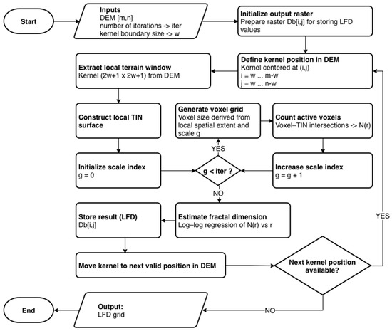
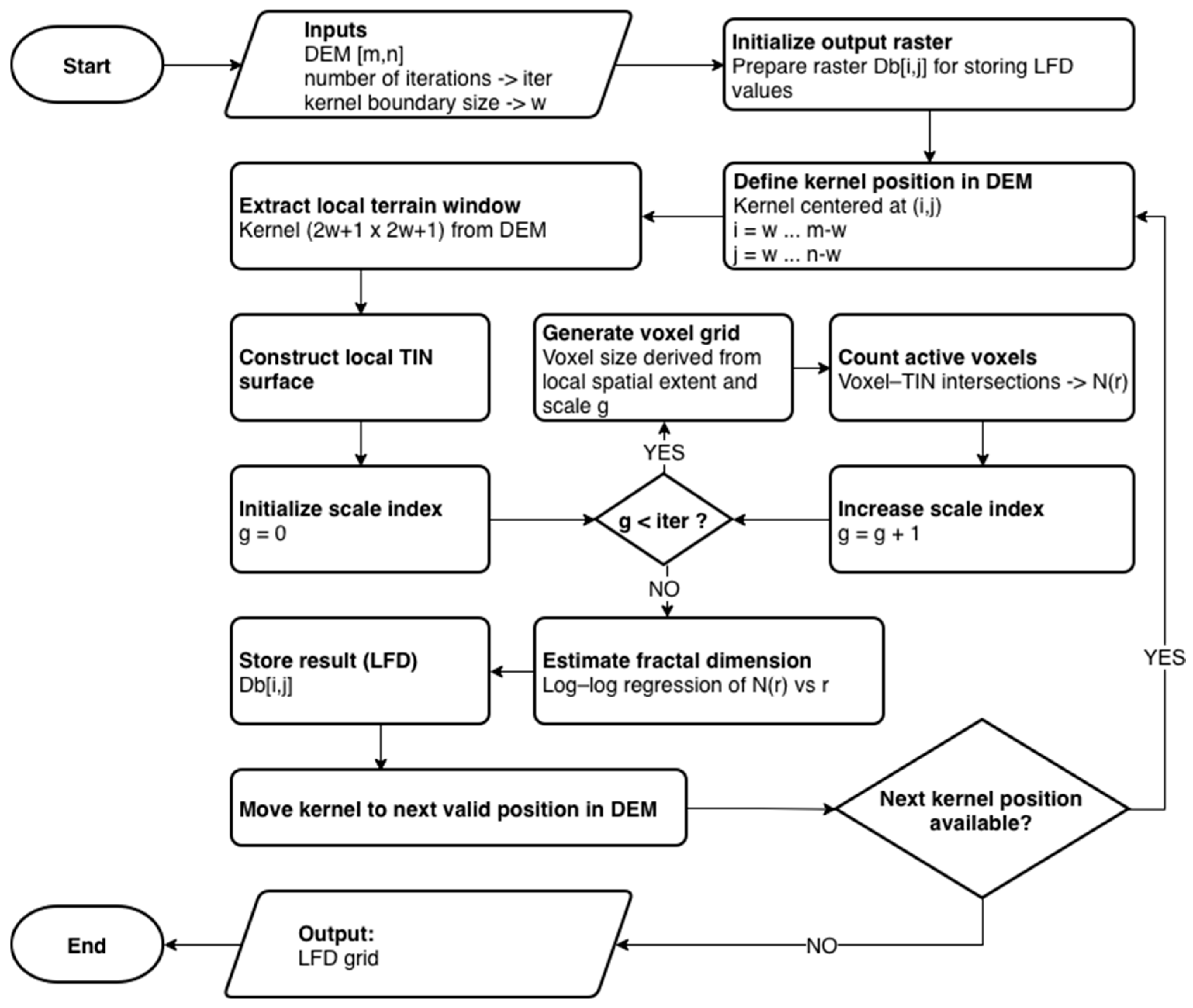
The calculation of the LFD is presented in Figure 3. It is based on dividing the analysed space into a regular 3D voxel grid and determining the intersection of these voxels with a surface represented by a Triangulated Irregular Network (TIN) generated via Delaunay triangulation [61]. This method ensures comprehensive 3D surface modelling suitable for FD computation using the box-counting method, although it can be time-consuming and computationally intensive. For example, a 3D box-counting method was also used in [62].
Figure 3.
Flowchart of the methodology used for LFD calculation.
Intersection detection between voxels and the triangular facets of the TIN model is performed using an algorithm grounded in the Separating Axis Theorem, as described by Ericson [63] and Akenine-Möller et al. [64]. This algorithm tests potential separating axes—13 in total—to determine if the voxel (box) and triangle intersect. The existence of at least one separating axis indicates that the objects do not overlap [63,64,65]. These theoretical principles were implemented in a custom Python script by Ič [15] for calculating the parameter .
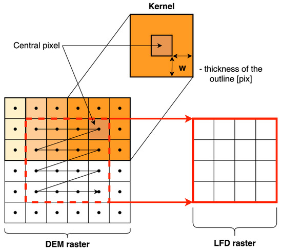
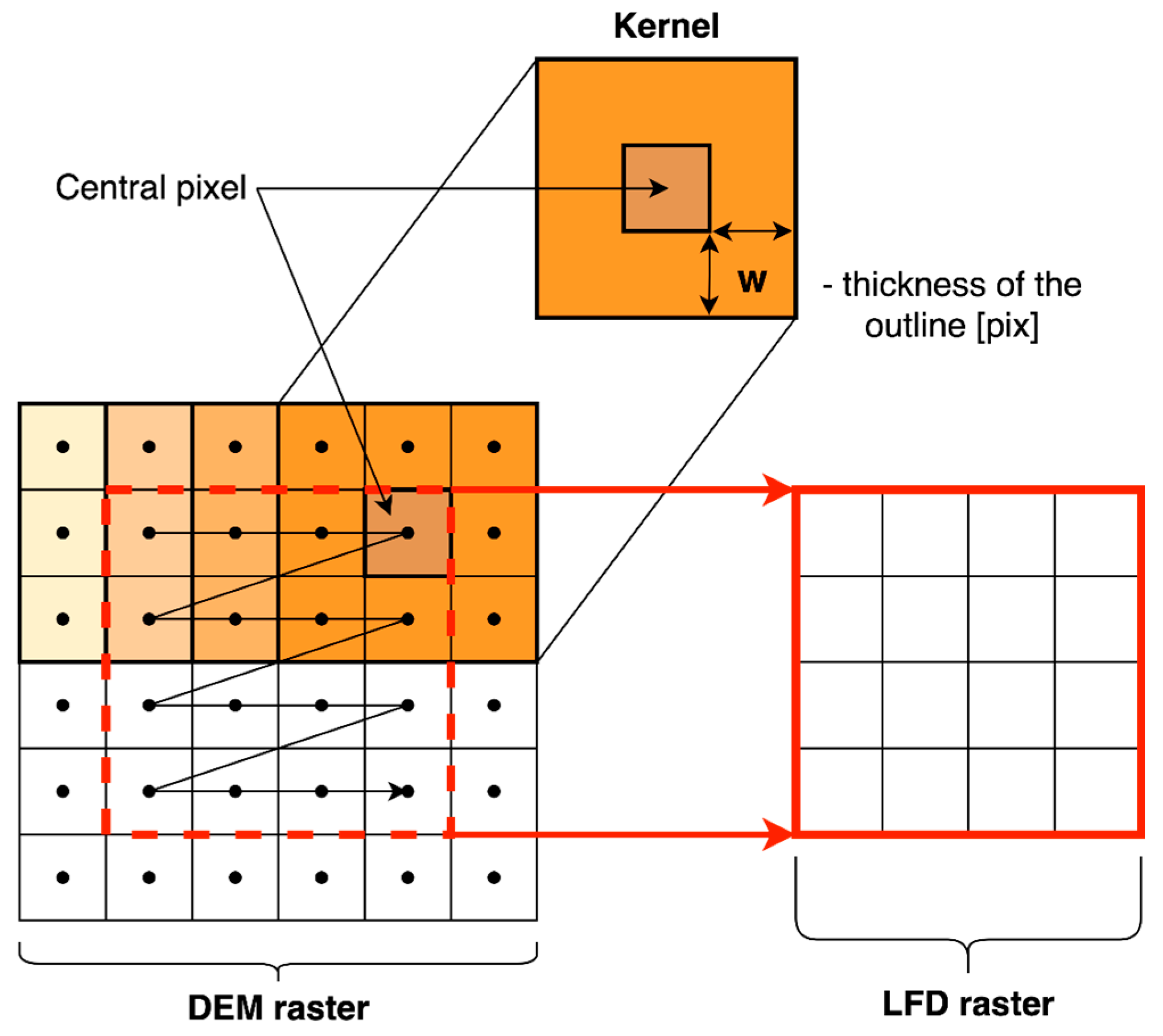
The LFD calculation, like that of other roughness parameters, is performed using a moving computational window (kernel) that defines the local neighbourhood around each central raster pixel (Figure 4). The kernel size can be increased to include more distant pixels, enabling FD to reflect a broader surrounding context. However, enlarging the kernel also introduces a degree of generalisation into the resulting LFD values.
Figure 4.
Principle of LFD calculation using a moving computational window, according to [15].
Since the box-counting algorithm operates iteratively, within each kernel, for every iteration with a different scale r, the number of active voxels N(r) containing triangles from the TIN model is counted. The number of iterations is an adjustable parameter depending on the desired level of analytical detail. The box sizes decrease geometrically with each iteration, typically halving in size. Based on the relationship between N(r) and r, the box-counting dimension is estimated via linear regression in log–log space (Figure 3). This dimension corresponds to the slope of the regression line fitted to the values of N(r) versus r [57].
The output of the LFD calculation is a raster layer containing the LFD values for each pixel and its neighbourhood. This method was implemented using custom Python tools, as it is not commonly available in GIS software environments.
The smallest possible computational window is 3 × 3, which we included in our study for each parameter calculation as the most basic and simplest option. This window is the least computationally demanding, but it only includes the closest neighbourhood of each point. Therefore, the optimal kernel size for roughness calculation was determined based on an analysis of the MSR output implemented in WhiteboxTools within the QGIS environment. Specifically, the scale raster was evaluated, which records, for each grid cell, the neighbourhood size at which the maximum roughness value is attained, considering scales up to a maximum of 15 cells. The frequency distribution (histogram) of scale values indicated that the most prevalent scales range between 2 and 5 cells, with peaks at 2–3 cells in high-mountain area and around 3 cells in the urban area. These values represent the dominant spatial scales at which terrain variability is most pronounced within the study area. These scales correspond to kernel sizes ranging from 3 × 3 to 9 × 9 cells, which were subsequently selected as the window sizes for roughness calculation.
To ensure a fair comparison, we also used these calculation windows to compute the MSR and TRI parameters (Section 2.4.2 and Section 2.4.3).
2.6. Potential Solar Radiation
In this study, we calculated the potential annual global solar radiation using the Area Solar Radiation (ASR) tool within the ArcGIS Pro (part of the Spatial Analyst) [66], based on DTM and DSM with resolutions of 1 m, 5 m and 25 m. The ASR tool uses latitude and longitude, elevation, slope, aspect, and atmospheric transmissivity as its primary input parameters [66,67], typically derived from input terrain and location data. Default parameter values were applied for all settings, except for latitude, which was automatically determined based on the study area’s location, and the time interval was adjusted from 0.5 h to 1 h to reduce computational load (Table 1). Note that in this study, we did not focus directly on calculating PSR, i.e., its absolute values, but rather on its changes and relative values with respect to the surroundings of a given location. For this type of analysis, it is especially important that the parameters are set the same in all calculations. Therefore, we do not deal with tuning these values for specific situations in this article.
Table 1.
The input parameters in the calculation of PSR using the Area Solar Radiation tool.
Other tools for PSR calculating include r.sun [68,69] and the Point Cloud Solar Radiation Tool (PCSRT) [70]. The ASR and r.sun tools are suitable for large-area calculations, utilising DTM or DSM for modelling. In contrast, the PCSRT enables higher-precision PSR calculations within a 3D space, working directly with point cloud data obtained, for example, from ALS [70]. This tool models PSR in more detail but is also more computationally demanding. Therefore, one of our goals is to more precisely identify areas where a more accurate tool for PSR calculation is needed and where less detailed modelling with lower raster resolution is sufficient. We aim to determine these areas based on surface roughness and propose grouping or reclassifying regions with higher roughness into appropriate categories (Section 2.7).
2.7. Cross-Correlation Analysis of Terrain Parameters, Surface Roughness, and Uncertainties in PSR Calculation
To assess the impact of surface roughness on the accuracy of PSR estimation, we first calculated the absolute differences between PSR models derived at different resolutions, as well as the differences between PSR models computed from DTM and DSM data. We then generated a correlation matrix using the Pearson correlation coefficient [71], encompassing all terrain parameters, roughness parameters, and PSR estimation uncertainties, to explore their interrelationships. The primary objective was to identify dependencies among roughness parameters, with particular emphasis on their influence on the accuracy of PSR calculations. Basic raster correlations can be computed using the Band Collection Statistics tool in ArcGIS [71,72]; however, we also developed and applied a custom Python script, including the calculation of p-values, confidence intervals, Moran’s I, permutation tests, and multicollinearity diagnostics. Before the calculations, we removed a 100 m buffer from the edges of all rasters to avoid potential inaccuracies caused by missing or unreliable edge values that could negatively affect the results.
2.8. Surface Reclassification and Clustering by Roughness
For visual comparison of the results, we recommend using the quantile method to reclassify both roughness and PSR calculation errors. This approach allows the identification and comparison of the roughest areas, independent of the specific numerical values. As a more advanced solution, considering spatial relationships, clustering by roughness metric can be used (e.g., using the K-means method) [73].
Then, in the roughest terrain, we recommend calculating PSR directly from the high-resolution DSM, or even from the point cloud data itself [70], in accordance with [5]. In less rugged areas, lower-resolution models suffice, and PSR can be estimated using software tools such as ASR, r.sun [68,69], or by applying calculations based on DTM instead of DSM (for example, when an actual DSM from the desired time period is not available).
3. Results
3.1. Terrain Parameters, Surface Roughness, and PSR Calculations
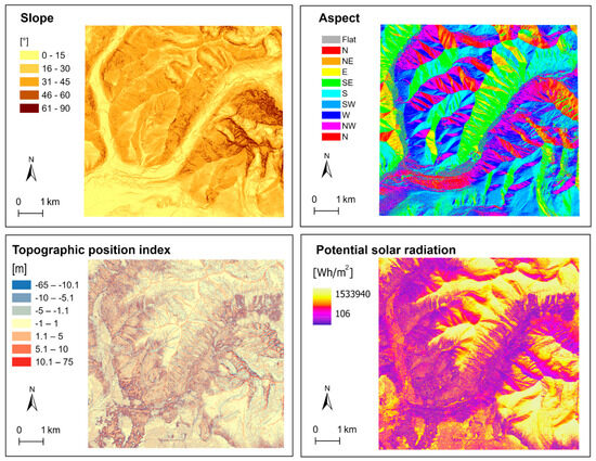
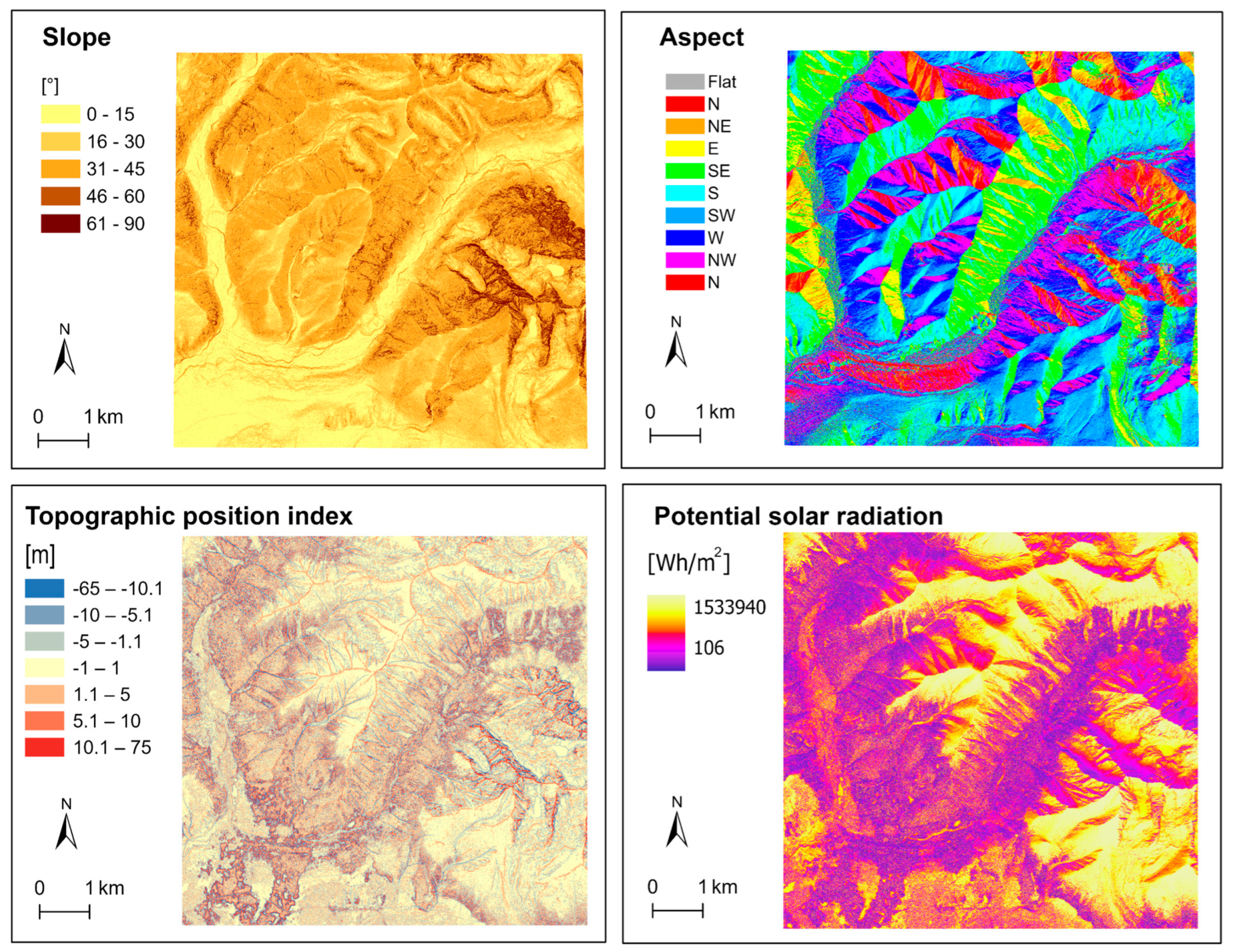
The results of the calculated basic terrain parameters (Section 2.3) and PSR (Section 2.6) from the area of the first case study are shown in Figure 5. Their visualisation, alongside Figure 1, helps to more clearly illustrate the characteristics of the tested alpine terrain.
Figure 5.
Case study in the High Tatra Mountains: Basic terrain characteristics and PSR calculated using 1 m resolution DTM and DSM. The TPI parameter was computed using a 9 × 9 kernel. All parameters are calculated in ArcGIS Pro.
Since the 1 m resolution captures local roughness at the scale of individual trees, we selected a spatial resolution of 5 m as the baseline for further analyses (see Appendix A). Moreover, there is no reason to assume that a finer spatial resolution will always improve accuracy, as it may also introduce noise. Some processes may be evident at certain spatial scales but not at others.
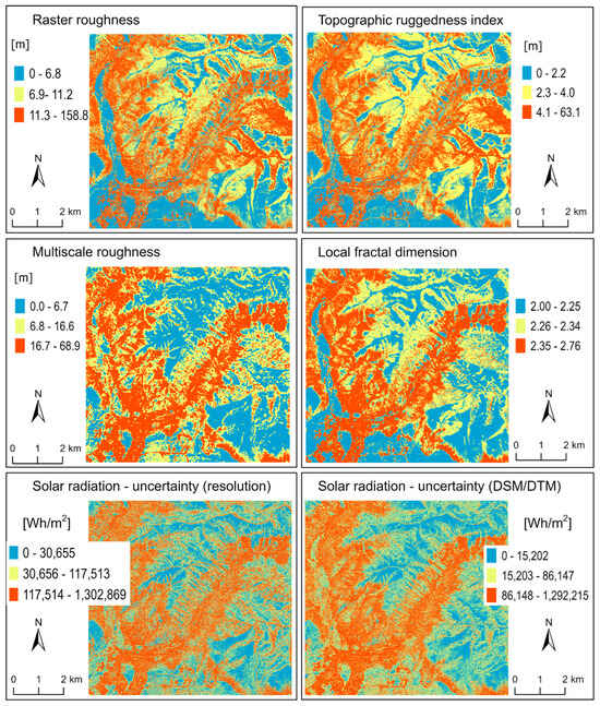
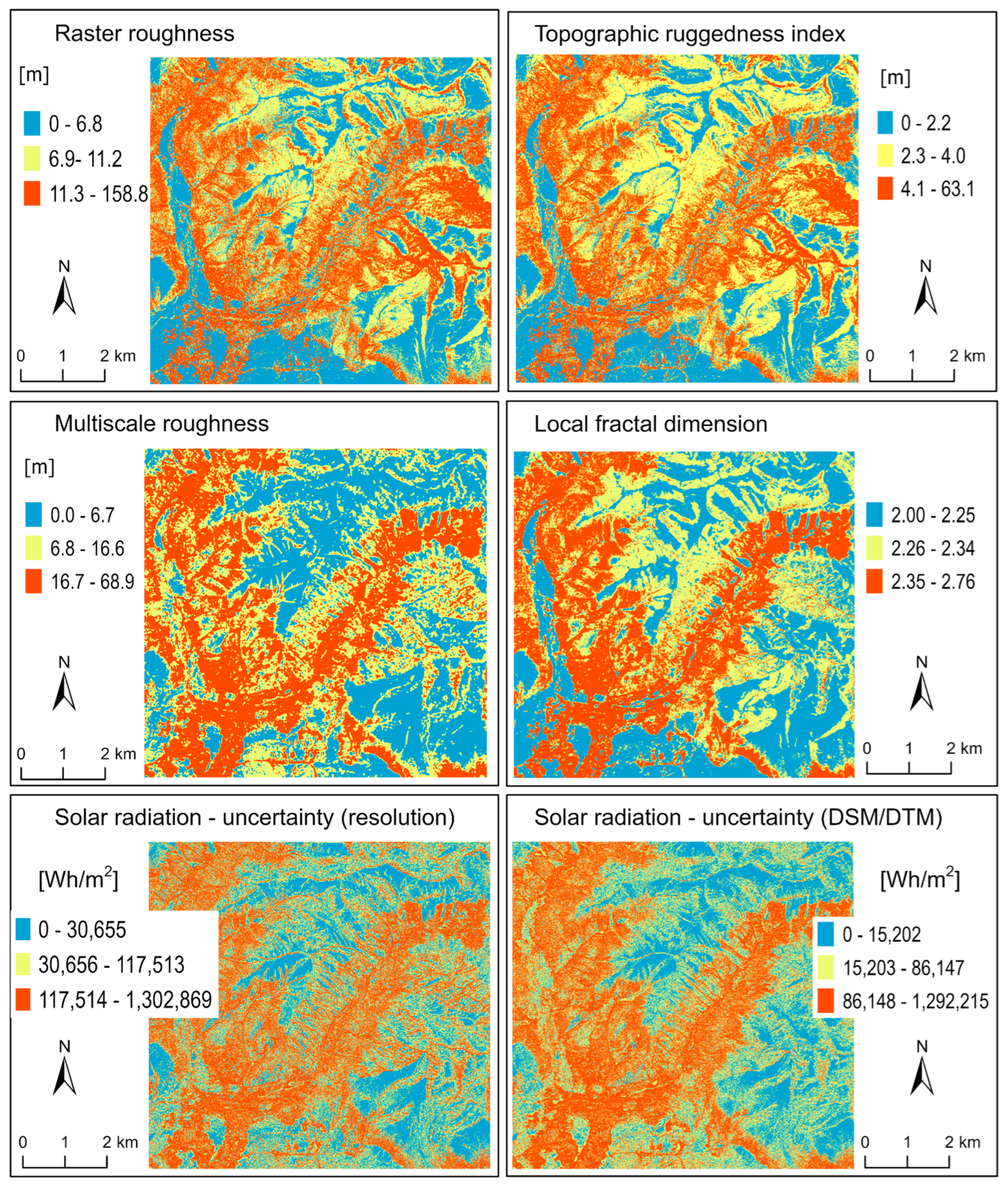
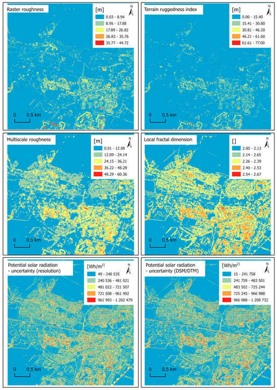
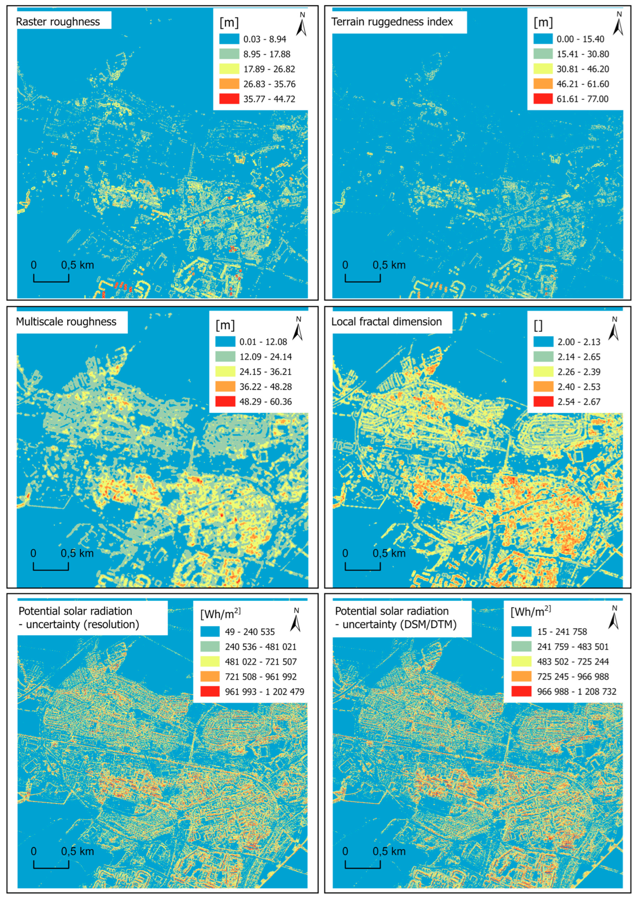
Figure 6 shows a visualisation of all the tested roughness parameters, RR, TRI, MSR, and LFD, from the area of the first case study. For better visual comparison despite the different value scales, we reclassified them all using three quantiles. This method assigns the same number of elements to each category, allowing for easy visual comparison of the results. The inaccuracies or uncertainties in the calculation of PSR caused by the reduced resolution and the difference between DSM and DTM are shown in Figure 6 below. The results exhibit a high degree of visual similarity, despite differences in numerical values and the specific methods applied.
Figure 6.
Case study in the High Tatra Mountains: Visualisation of reclassified roughness indices (top and middle) and the inaccuracies (uncertainties) in PSR calculation caused by reduced resolution (bottom left) and by the difference between DSM and DTM (bottom right). Three-quantile reclassification was used for better comparison.
Note that Figure 6 shows LFD calculated from the DSM at a spatial resolution of 5 m; however, we also analysed LFD computed at a resolution of 1 m and using the DTM. The corresponding results are provided in Appendix A (Figure A1 and Figure A2).
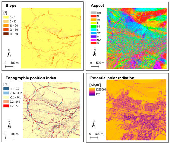
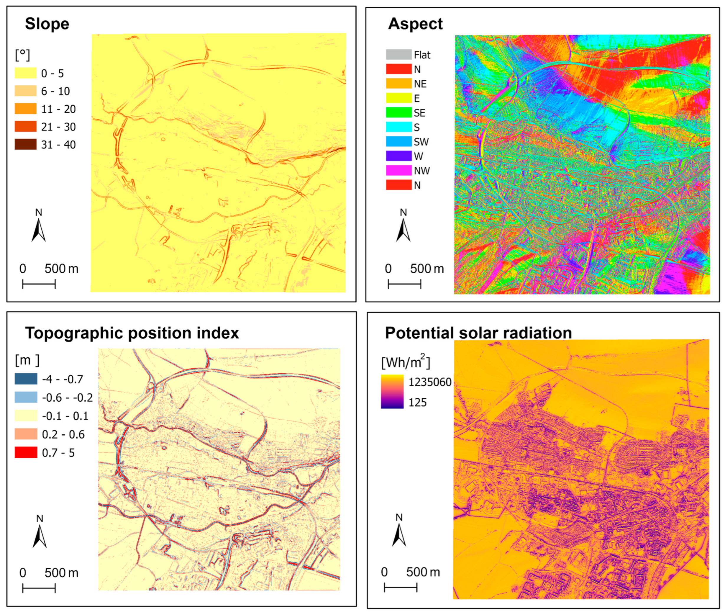
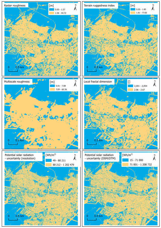
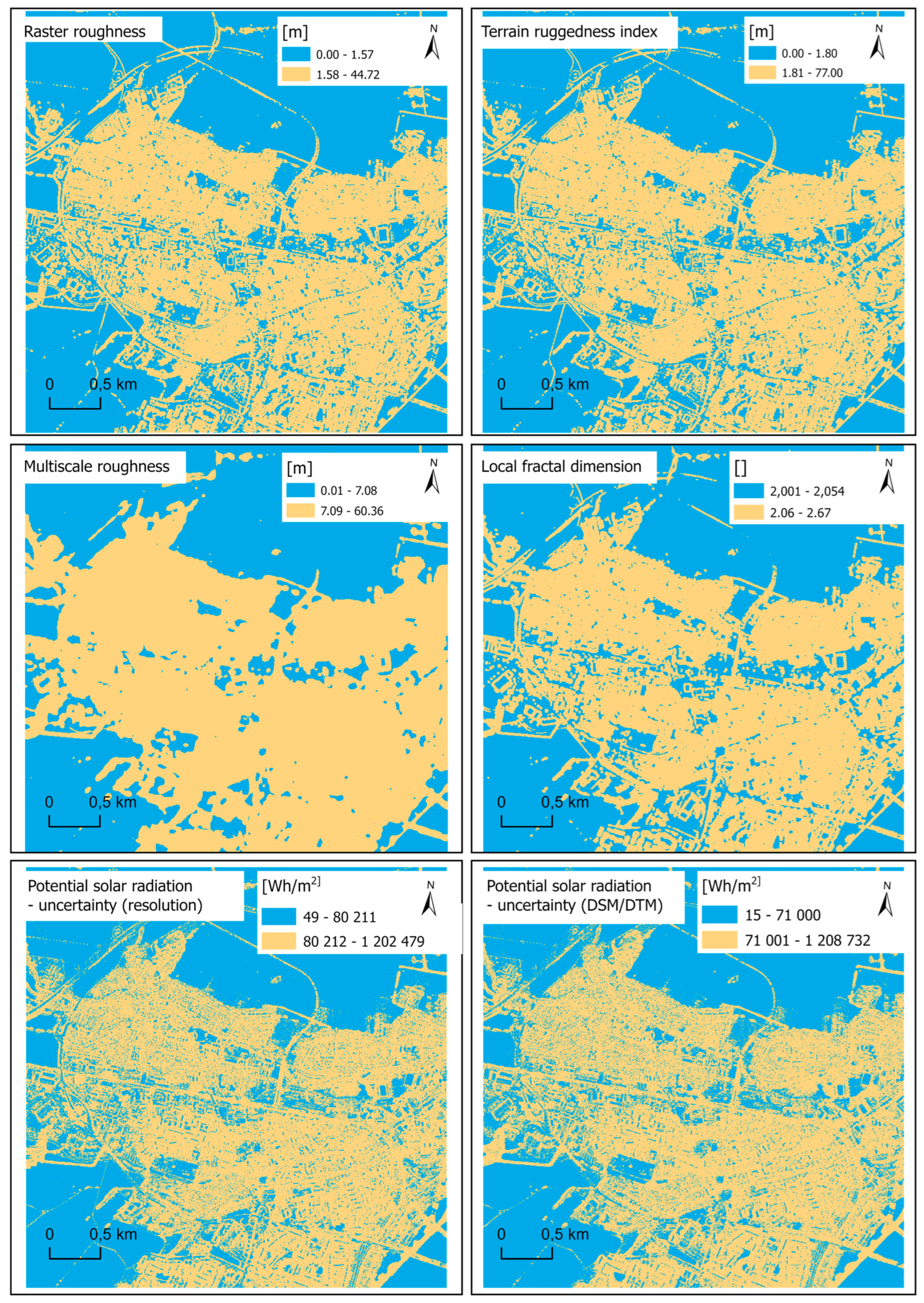
The results of second case study are visualised in Figure 7 and Figure 8. Note that for the Poprad area, two classes were used for visual comparison instead of three due to the predominance of low values in the RR and TRI parameters. This issue did not occur in the more rugged Tatra Mountains, where three classification classes were used.
Figure 7.
Case study of Poprad: Basic terrain characteristics and PSR calculated using 1 m resolution DTM and DSM. The TPI parameter was computed using a 9 × 9 kernel.
Figure 8.
Case study of Poprad: Visualisation of the roughness parameters (top and middle) and uncertainties in the calculation of potential solar radiation (bottom).
A visual comparison in both case studies suggests that higher uncertainties are associated with rougher surface; however, we further seek to confirm this relationship by calculating correlation coefficients and conducting multicollinearity tests (Section 3.2).
3.2. Calculating Correlations and Multicollinearity Tests
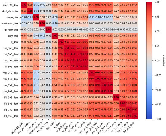
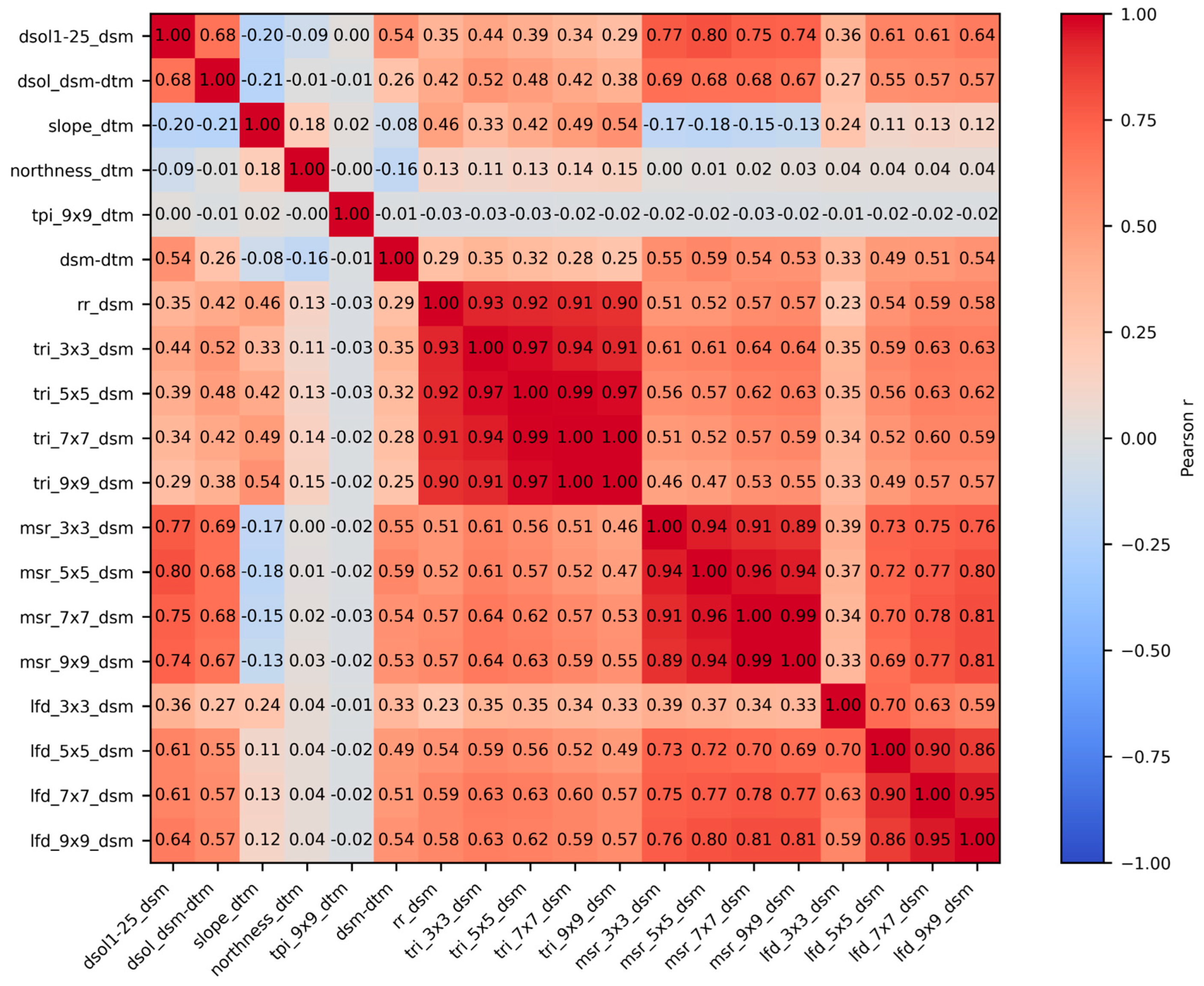
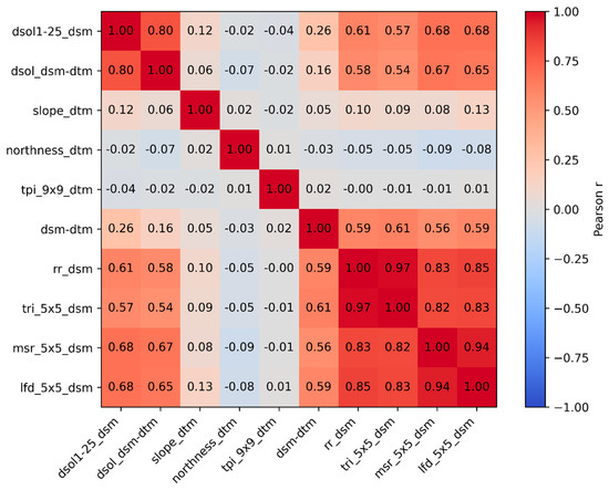
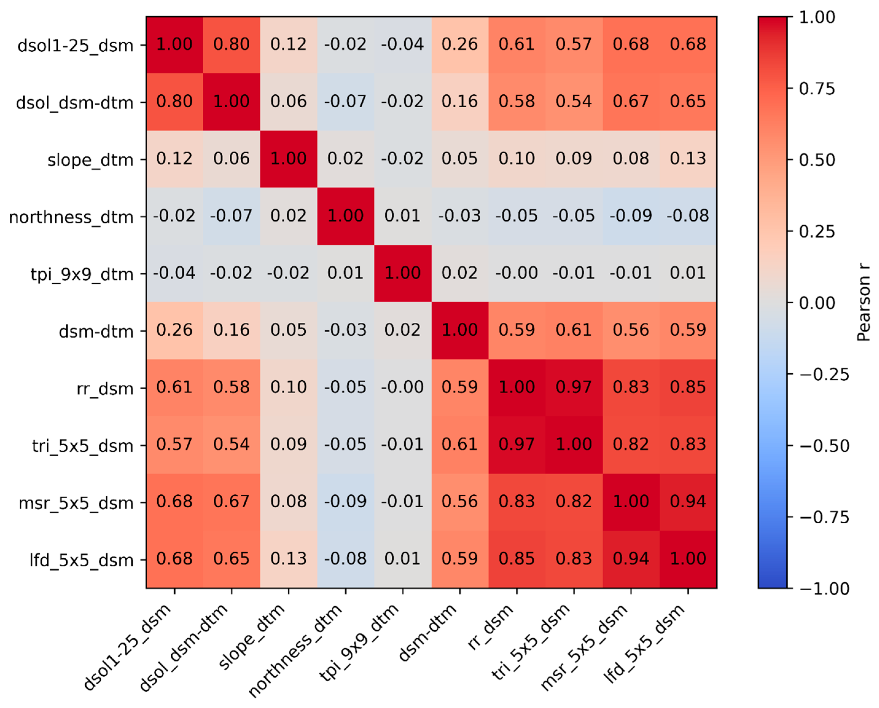
Visual comparison between the reclassified roughness indices and the uncertainties in PSR calculations suggested a strong agreement between the two (Figure 6 and Figure 8). This finding suggests that surface roughness influences the magnitude of uncertainties in calculating PSR, in line with our initial hypothesis. To further investigate this relationship, we calculated pairwise Pearson correlation coefficients (r values) among all main examined parameters (Table 2). This result was obtained as a direct output of our custom Python script, which was written and used for the calculation of correlations, p-values, confidence intervals, Moran’s I, permutation tests to derive empirical p-values, and multicollinearity tests. For better clarity, the results are presented in the form of colour-visualised correlation matrices of all (Figure 9) or the most significant parameters (Figure 10). Note that all reported correlations were statistically significant (p < 0.05). The results of the statistical analysis are provided in Supplementary Materials. Given the large sample size (2,431,995 and 556,516 raster cells), all correlations are statistically significant with narrow 95% confidence intervals; therefore, the interpretation focuses primarily on the magnitude of the correlation coefficients rather than on p-values alone.
Table 2.
Analysed parameters: PSR calculation uncertainties (1–2), terrain parameters (3–6), and surface roughness (7–16).
Figure 9.
Heatmap of the correlation matrix for the first case study, illustrating the relationships among PSR calculation uncertainties, terrain parameters (slope, northness, TPI, difference between DSM and DTM), and surface roughness parameters (RR, TRI, MSR, and LFD).
Figure 10.
Heatmap of the correlation matrix for the second case study, showing the relationships between PSR calculation uncertainties, terrain parameters (slope, northness, TPI, difference between DSM and DTM), and the most suitable versions of surface roughness parameters (RR, TRI, MSR, and LFD).
Moran’s I values ranged from 0.51 to 0.99, indicating the presence of spatial autocorrelation in all analysed variables. Moderate spatial autocorrelation was observed for slope, northness, and TPI, whereas terrain roughness indices (e.g., TRI and RR) exhibited strong spatial clustering. Extremely high spatial autocorrelation was detected for MSR (I = 0.99) and LFD (I = 0.97), reflecting highly spatially structured surfaces (Supplementary Materials).
These results confirm that the analysed variables are not spatially independent, thereby violating the assumptions of classical correlation analysis.
To account for spatial autocorrelation, the statistical significance of Pearson correlation coefficients was evaluated using a permutation-based approach (n = 500 permutations). Permutation tests were used to derive permutation-based p-values. All correlations remained statistically significant (p ≤ 0.004 for the Tatra Mountains and p ≤ 0.002 for the Poprad area), indicating that the observed relationships are robust and not solely driven by spatial structure. This approach provides a more reliable assessment of statistical significance in spatially structured data compared to standard parametric tests
Some surface roughness metrics, particularly MSR and LFD, exhibit very strong mutual correlations, with Pearson correlation coefficients ranging from 0.82 to 0.94, indicating that the different methods capture closely related aspects of terrain roughness. In contrast, the correlations between the roughness metrics and other terrain parameters are mostly negligible, suggesting that surface roughness represents a largely independent terrain characteristic rather than a simple derivative of conventional topographic variables. At the same time, the correlations between the roughness metrics and PSR calculation uncertainties reach strong values (r = 0.61–0.80), suggesting that surface roughness plays an important role in the magnitude of uncertainties in PSR modelling.
The variance inflation factor (VIF) values between the roughness parameter and the other variables reached a maximum of 1.19 when using LFD and 1.22 when using MSR, indicating no problematic collinearity between the roughness parameters derived in these ways and the remaining terrain parameters.
3.3. Clustering and Reclassification
The results suggests that surface roughness is an important factor influencing PSR calculation, as expected. Therefore, we propose identifying areas with higher roughness as zones where PSR should be modelled with increased caution. Such areas can be delineated using reclassification or clustering approaches.
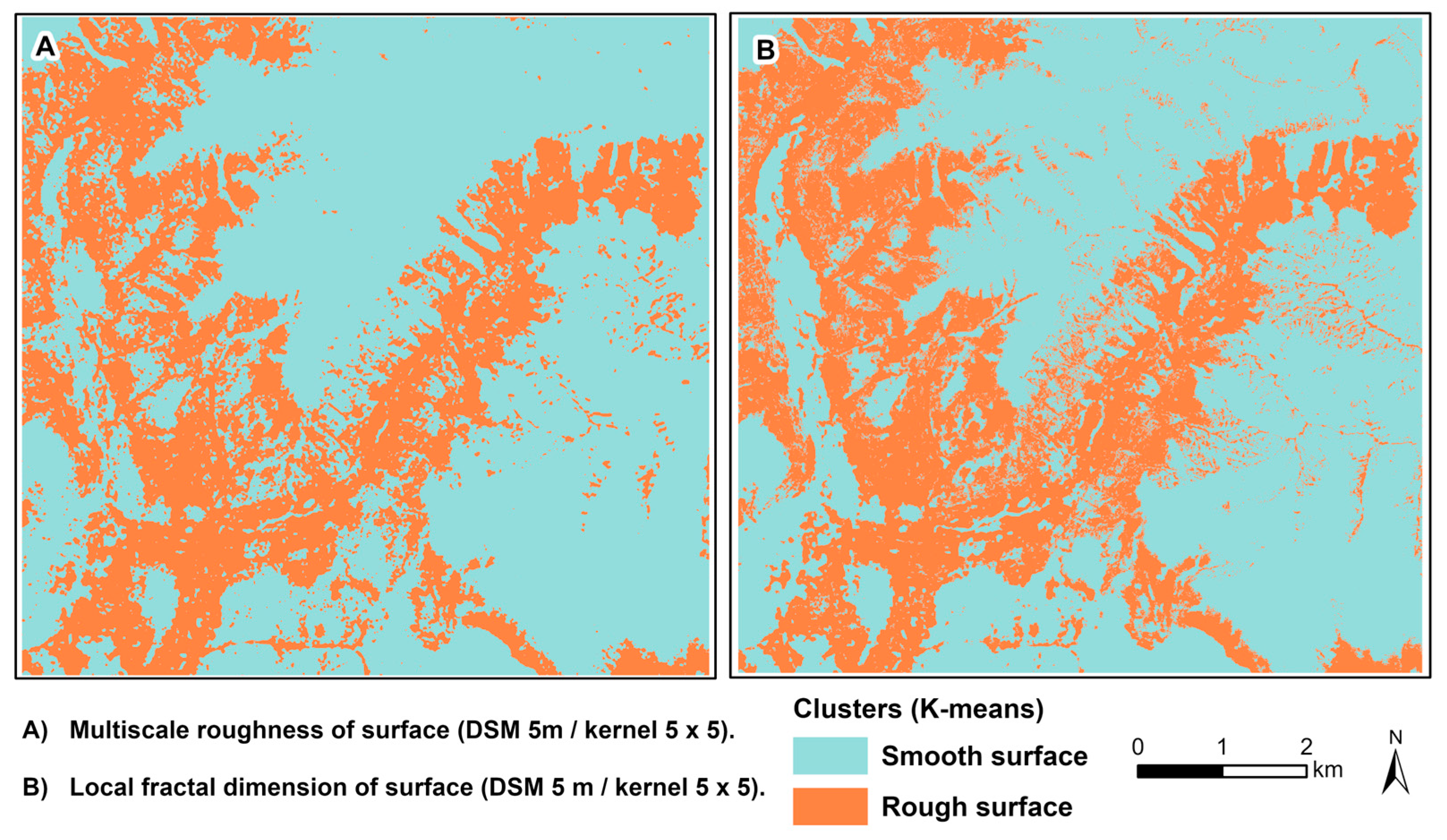
A reclassification of the results using three-quantile (Figure 6) and two-quantile (Figure 8) reclassification was performed using ArcGIS Pro. Clustering of roughness values using the K-means method [73] is presented in Figure 11. In this study, for example, we used K-means clustering for grids from SAGA Next Gen tools and the Iterative Minimum Distance method [73] with 100 iterations and periodical start partition. For this visualisation, we used the MSR and FD values calculated with the 5 × 5 m kernel; however, these could be replaced with any other roughness parameter if needed. To better demonstrate the results, we used only two categories (clusters): smooth surface (low roughness) and rough surface (high roughness). The clustering method, criteria for creating categories, as well as the number of categories, can, of course, be adapted to the specific case study.
Figure 11.
Clustering into two categories according to MSR and LFD using the K-means method.
4. Discussion
4.1. Modelling Surface Roughness in GIS
The first objective of this work was to review the current availability of methods and software tools for calculating surface roughness in GIS environments and to assess their independence from other terrain parameters. We applied the RR, TRI, MSR metrics and additionally designed and implemented a new LFD parameter.
It is noteworthy that the roughness parameters exhibited high mutual correlations despite being calculated using different methods, which is expected if they indeed represent surface roughness. The Pearson correlation coefficients range from 0.57 to 0.97 (Figure 9 and Figure 10), suggesting a high degree of consistency among the different approaches In particular, very high intercorrelations are observed in the urban environment (0.82–0.97).
Figure 9 and Figure 10 also show low correlations between parameters such as slope, aspect (northness), and TPI and roughness, as well as among these terrain parameters themselves. This finding is further supported by the calculated VIF values, which did not exceed 1.22. In our study, some surface roughness parameters (particularly MSR and LFD) were found to be independent of slope, aspect, and TPI even in mountainous environments (Figure 9), suggesting their direct applicability as additional characteristics to terrain parameters in predictive models and analyses [37,74]. In contrast, other roughness parameters, mainly those based on the height difference between the central cell and its surroundings, do not share this advantage. In urban environments, the situation is different, as surface roughness is mainly controlled by buildings and other above-ground objects. In this case, all roughness parameters appear to be independent in relation to the analysed terrain characteristics (Figure 10). This observation is particularly important when selecting parameters for predictive modelling approaches that require independence of input variables.
4.2. LFD as a New Roughness Parameter
Although LFD provides a spatially explicit characterisation of surface roughness, it is computationally more demanding than standard GIS roughness metrics, as it requires testing intersections between voxels and triangles within a moving window (Figure 3). For example, the LFD calculation for the Poprad city case study (5 × 5 kernel) took 14 h 37 min 51 s, using 10 cores in parallel on a 2.6 GHz 6-core Intel Core i7 processor with 16 GB of 2667 MHz DDR4 memory. As expected, computation time increases with the number of raster cells, the size of the applied kernel, and the number of iterations used in the local box-counting calculation.
Despite its higher computational demands, LFD remains a valuable method for characterising local heterogeneity and multiscale structure. This statement is supported by the high mutual correlations of the applied roughness parameters, especially between MSR and LFD, even though the mathematical principles of both methods are different (the correlation coefficient reached 0.81 in the mountainous environment and 0.94 in the urban environment). However, in its current implementation, the application of LFD calculation to large regional models may be impractical or even infeasible without parallel processing or GPU optimisation. In contrast, the MSR method uses a fast integral image approach to efficiently compute these values across different computational window sizes [12]. Therefore, further streamlining of LFD computation will be required in the future to make it a fully operational surface roughness parameter.
4.3. Assessment of the Impact of Surface Roughness on Potential Solar Radiation Calculation
Another motivation for this study was to demonstrate that it is not sufficient to rely solely on simple, commonly used roughness parameters such an RR and TRI when modelling the influence of surface roughness on phenomena such as solar radiation (Figure 9 and Figure 10). Among the tested parameters, MSR and LFD with 5 × 5 to 9 × 9 kernels (corresponding to 25–45 m in this study) emerged as the most suitable for this purpose (correlations from 0.55 to 0.80). It is important to emphasise that errors in PSR calculations often occur near complex or rough features that cast shadows or obscure surrounding areas. As a result, correlation analyses that consider only cell-to-cell dependencies tend to underestimate the true extent of these dependencies. This is particularly evident in urban environments, which could also have caused lower values of correlation coefficients than in mountainous environments. Another finding is that a small kernel at high resolution (1 m) fails to capture the surrounding roughness, considering only local features (e.g., individual trees in a forest, Figure A2 in the Appendix A). Therefore, we did not use the 1 m resolution relief roughness in the correlation analyses. However, we can also agree with [12,13] that there is no single optimal kernel size or surrounding area that can be chosen to characterise topographic texture, including surface roughness. Several other studies also underscore the necessity of a multiscale approach and the careful selection of computational kernels, as results heavily depend on these methodological choices [12,28,55]. Following Berti et al. [49], we can also conclude that in analyses of this type, data resolution and computational window size are sometimes more critical than the specific algorithm used for roughness calculation.
Like our study, Wang and Wang [75] emphasise the importance of considering surface roughness when calculating some derived parameters. While it is known that solar radiation modelling is more challenging in rougher terrain [70], the contribution of this paper is also to provide a method to effectively identify these areas. A simpler but less accurate alternative is to use the direct difference between the DSM and DTM (normalised DSM). However, this approach primarily captures vegetation and building heights rather than representing overall surface roughness. In forested areas, this difference may still correlate with surface roughness parameters, but it does not provide a comprehensive measure of terrain complexity. Moreover, in an urban environment, this parameter is completely useless for this purpose (correlation coefficients 0.16 and 0.26). A visual comparison of DSM and DTM differences and roughness maps (Figure 1, Figure 6 and Figure 8) also demonstrates that elevation model differences primarily capture vegetation-induced roughness, whereas roughness parameters such as MSR and LFD reflect both vegetation and terrain roughness. This suggests that roughness metrics are more suitable parameters for refining the accuracy of solar radiation estimation.
A minor limitation of this study is that it was conducted on relatively small areas, with a total extent of 80 km2; however, the analysis includes both high-mountain and urban environments, and the selected areas represent both smoother and rougher terrain types.
5. Conclusions
This study evaluates surface roughness metrics in GIS environments and introduces a new parameter, the local fractal dimension (LFD). Surface roughness parameters such as Multiscale Roughness (MSR) and LFD were found to be independent of slope, aspect, and topographic position index (TPI), making them valuable supplementary metrics for various spatial analyses and predictive modelling tasks. While LFD shows considerable potential, MSR computed using WhiteboxTools is currently recommended as a more computationally efficient and accessible roughness metric.
This study also suggests that surface roughness has a substantial influence on the accuracy and uncertainty of potential solar radiation (PSR) modelling in both high-mountain and urban environments—particularly when the resolution of input rasters is reduced or when discrepancies exist between DSM and DTM. In general, surface exerts a greater influence on PSR uncertainties than DSM–DTM differences themselves.
Given the computational cost of solar radiation modelling, roughness parameters provide a practical means to classify terrain and identify areas where high-resolution modelling is essential versus where coarser models may suffice. Nevertheless, careful selection of raster resolution and computational window size remains essential for achieving accurate modelling results.
Supplementary Materials
The following supporting information can be downloaded at https://www.mdpi.com/article/10.3390/ijgi15040155/s1.
Author Contributions
Conceptualisation, Renata Ďuračiová and Tomáš Ič; methodology, Renata Ďuračiová and Tomáš Ič; software, Renata Ďuračiová and Tomáš Ič; validation Renata Ďuračiová, Tomáš Ič and Tomasz Oberski; formal analysis, Renata Ďuračiová and Tomáš Ič; investigation, Renata Ďuračiová, Tomáš Ič and Tomasz Oberski; resources, Renata Ďuračiová and Tomáš Ič; data curation, Renata Ďuračiová; writing—original draft preparation, Renata Ďuračiová and Tomáš Ič; writing—review and editing, Renata Ďuračiová, Tomáš Ič and Tomasz Oberski; visualisation, Renata Ďuračiová and Tomáš Ič; supervision, Renata Ďuračiová; project administration, Renata Ďuračiová; funding acquisition, Renata Ďuračiová. All authors have read and agreed to the published version of the manuscript.
Funding
This research was funded by the Slovak Research and Development Agency under Contract No. APVV-22-0151 and by grant No. VEGA 1/0626/25 of the Scientific Grant Agency of the Ministry of Education, Science, Research, and Sport of the Slovak Republic and the Slovak Academy of Sciences.
Data Availability Statement
The input data was available at: https://www.skgeodesy.sk/ (accessed on 12 December 2024). The data are freely available, but the user is obliged to state the source as follows: “ÚGKK SR”. The Python code implementing the LFD computation is available from Tomáš Ič upon reasonable request, while the Python code used for the statistical analysis is available from Renata Ďuračiová upon reasonable request.
Acknowledgments
During the preparation of this article, the authors used ChatGPT-5.3 (OpenAI) for text revision and grammar checking purposes. The authors have reviewed and edited the output and take full responsibility for the content of this publication.
Conflicts of Interest
The authors declare no conflicts of interest.
Abbreviations
The following abbreviations are used in this manuscript:
| ALS | Airborne laser scanning |
| ASR | Area solar radiation |
| DSM | Digital surface model |
| DTM | Digital terrain model |
| FD | Fractal dimension |
| GCCA SR | Geodesy, Cartography and Cadastre Authority of the Slovak Republic |
| GIS | Geographical information system |
| GKÚ | Geodetic and Cartographic Institute Bratislava (in Slovak) |
| LFD | Local fractal dimension |
| MSR | Multiscale roughness |
| PCSRT | Point cloud solar radiation tool |
| PSR | Potential solar radiation |
| RMS | Root-mean-square |
| RR | Raster roughness |
| TPI | Topographic position index |
| TRI | Terrain ruggedness index |
| ÚGKK SR | Geodesy, Cartography and Cadastre Authority of the Slovak Republic (in Slovak) |
| VIF | Variance inflation factor |
Appendix A. Visualisation of Local Fractal Dimension (LFD) Calculated Based on Digital Terrain Model (DTM) and Digital Surface Model (DSM)
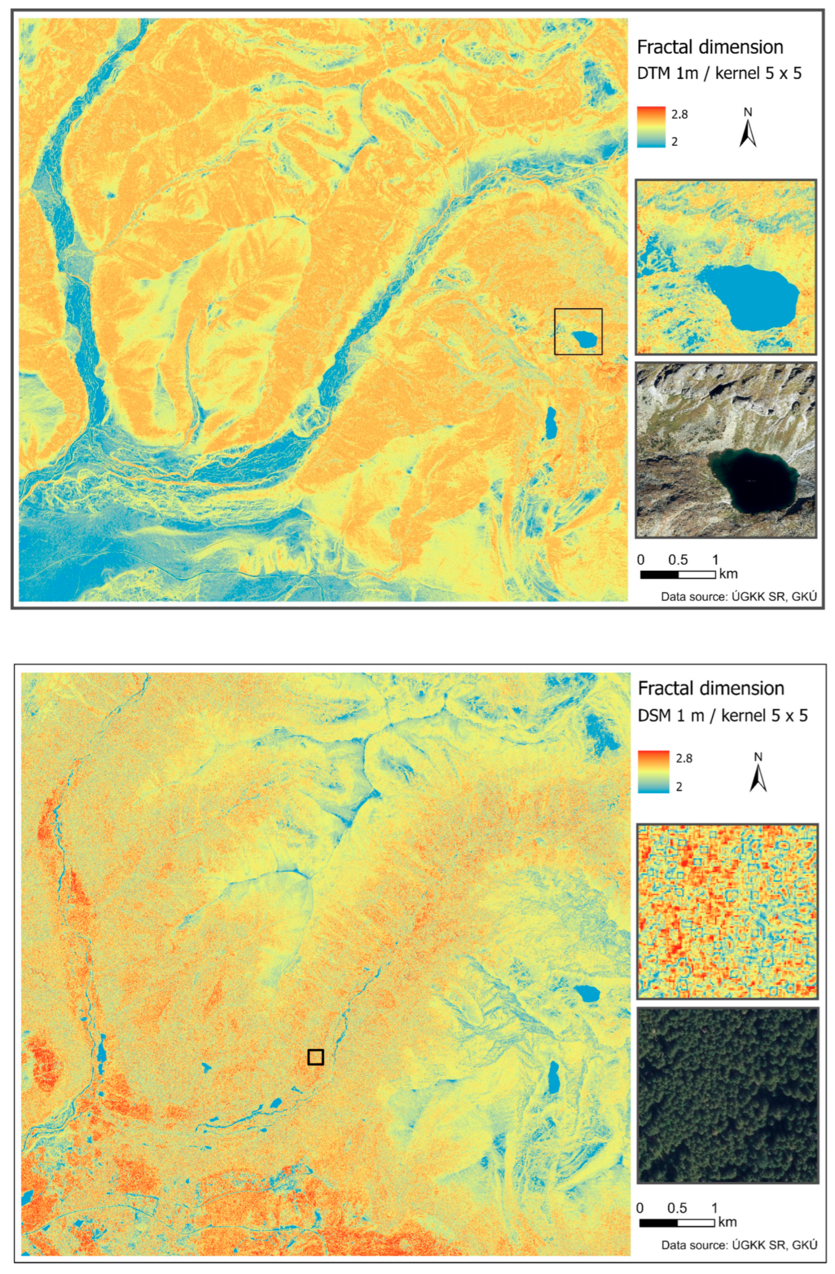
Figure A1 shows the LFD calculated based on DTM at a resolution of 5 m using a 5 × 5 m kernel. Figure A2 shows the LFD calculated based on DTM (top) and DSM (bottom) at a resolution of 1 m with a kernel of 5 × 5 m. Note that, for instance, water bodies exhibit the lowest fractal dimension (approximately 2), while rugged mountainous surfaces display the highest values. In these figures, we can also see that the LFD calculated on a 1 m resolution raster models local roughness at the tree level (Figure A2, top), not the surface as a whole; therefore, it seems more appropriate to use LFD calculated from a wider area or with a lower resolution (Figure A1).
Figure A1.
Example of the calculated LFD based on the 5 m resolution DSM using a 5 × 5 m kernel. In this case, valleys and meadows exhibit a lower LFD (blue) than mountains (orange to red).
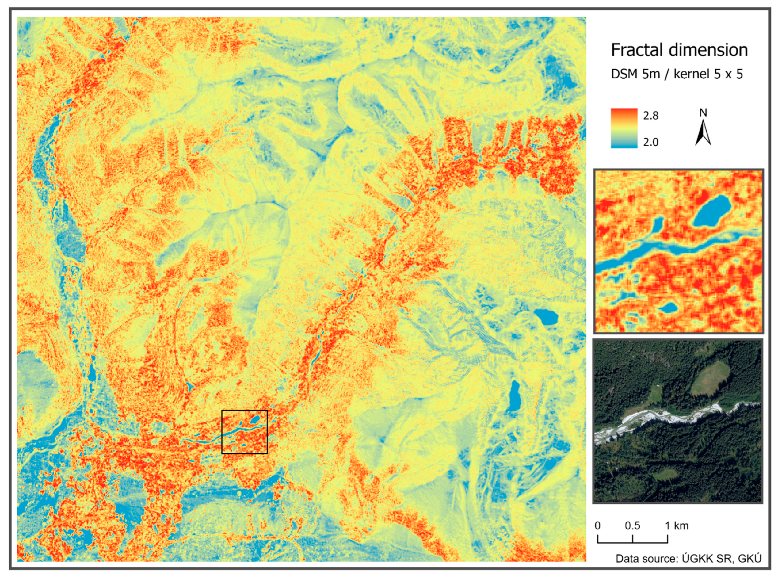
Figure A2.
Example of the calculated LFD calculated from a 1 m resolution DTM (top) and DSM (bottom) using a 5 × 5 m kernel. Water bodies exhibit the lowest fractal dimension values (approximately 2, shown in dark blue), whereas rugged mountainous surfaces (top) and vegetated areas with (bottom) display the highest values (orange to red).
References
- Tovar-Pescador, J.; Pozo-Vázquez, D.; Ruiz-Arias, J.A.; Batlles, J.; López, G.; Bosch, J.L. On the use of the digital elevation model to estimate the solar radiation in areas of complex topography. Meteorol. Appl. 2006, 13, 279–287. [Google Scholar] [CrossRef] [Scilit]
- Aguilar, C.; Herrero, J.; Polo, M.J. Topographic effects on solar radiation distribution in mountainous watersheds and their influence on reference evapotranspiration estimates at watershed scale. Hydrol. Earth Syst. Sci. 2010, 14, 2479–2494. [Google Scholar] [CrossRef] [Scilit]
- Flint, A.L.; Childs, S.W. Calculation of solar radiation in mountainous terrain. Agric. For. Meteorol. 1987, 40, 233–249. [Google Scholar] [CrossRef] [Scilit]
- Witzmann, S.; Gollob, C.; Kraßnitzer, R.; Ritter, T.; Tockner, A.; Schume, H.; Nothdurft, A. Modeling of solar radiation and sub-canopy light regime on forest inventory plots of mixed conifer and deciduous temperate forests using point clouds from personal laser scanning. For. Ecol. Manag. 2024, 569, 122166. [Google Scholar] [CrossRef] [Scilit]
- Buchalová, D.; Hofierka, J.; Šupinský, J.; Kaňuk, J. Estimating subcanopy solar radiation using point clouds and GIS-Based solar radiation models. Remote Sens. 2025, 17, 328. [Google Scholar] [CrossRef] [Scilit]
- Cenky, M.; Bendik, J.; Janiga, P.; Lazarenko, I. Urban-Scale Rooftop Photovoltaic Potential Estimation Using Open-Source Software and Public GIS Datasets. Smart Cities 2024, 7, 3962–3982. [Google Scholar] [CrossRef] [Scilit]
- Wilson, M.F.J.; O’Connell, B.; Brown, C.; Guinan, J.C.; Grehan, A.J. Multiscale Terrain Analysis of Multibeam Bathymetry Data for Habitat Mapping on the Continental Slope. Mar. Geod. 2007, 30, 3–35. [Google Scholar] [CrossRef] [Scilit]
- Riley, S.J.; De Gloria, S.D.; Elliot, R. A Terrain Ruggedness that Quantifies Topographic Heterogeneity. Intermt. J. Sci. 1999, 5, 23–27. [Google Scholar]
- Grohmann, C.H.; Smith, M.J.; Riccomini, C. Multiscale analysis of topographic surface roughness in the Midland Valley, Scotland. IEEE Trans. Geosci. Remote Sens. 2010, 49, 1200–1213. [Google Scholar] [CrossRef] [Scilit]
- Hani, A.F.M.; Sathyamoorthy, D.; Asirvadam, V.S. A method for computation of surface roughness of digital elevation model terrains via multiscale analysis. Comput. Geosci. 2011, 37, 177–192. [Google Scholar] [CrossRef] [Scilit]
- Smith, M.W. Roughness in the Earth sciences. Earth-Sci. Rev. 2014, 136, 202–225. [Google Scholar] [CrossRef] [Scilit]
- Lindsay, J.B.; Newman, D.R. Hyper-scale analysis of surface roughness. PeerJ Prepr. 2018, 6, e27110v1. [Google Scholar]
- Lindsay, J.B.; Newman, D.R.; Francioni, A. Scale-Optimized surface roughness for topographic analysis. Geosciences 2019, 9, 322. [Google Scholar] [CrossRef] [Scilit]
- Brožová, N.; Baggio, T.; D’Agostino, V.; Bühler, Y.; Bebi, P. Multiscale analysis of surface roughness for the improvement of natural hazard modelling. Nat. Hazards Earth Syst. Sci. 2021, 21, 3539–3562. [Google Scholar] [CrossRef] [Scilit]
- Ič, T. Local Modelling of the Fractal Dimension on Digital Elevation Models. In Juniorstav 2024: Proceedings 26th International Scientific Conference of Civil Engineering; Brno University of Technology, Faculty of Civil Engineering: Brno, Czech Republic, 2024; pp. 1–9. ISBN 978-80-86433-83-7. [Google Scholar] [CrossRef] [Scilit]
- Xu, T.; More, D.M.; Gallant, J.C. Fractals, Fractal Dimensions and Landscapes—A review. Geomorphology 1993, 8, 245–262. [Google Scholar] [CrossRef] [Scilit]
- Huang, J.; Turcotte, D.L. Fractal image analysis: Application to the topography of Oregon and synthetic images. J. Opt. Soc. Am. A 1990, 7, 1124–1130. [Google Scholar] [CrossRef] [Scilit]
- Hagerhall, C.M.; Purcell, T.; Taylor, R. Fractal dimension of landscape silhouette outlines as a predictor of landscape preference. J. Environ. Psychol. 2004, 24, 247–255. [Google Scholar] [CrossRef] [Scilit]
- Goff, J.A.; Tucholke, B.E. Multiscale spectral analysis of bathymetry on the flank of the Mid-Atlantic Ridge: Modification of the seafloor by mass wasting and sedimentation. J. Geophys. Res. 1997, 102, 15447–15462. [Google Scholar] [CrossRef] [Scilit]
- Gagnon, J.S.; Lovejoy, S.; Schertzer, D. Multifractal earth topography. Nonlinear Process. Geophys. 2006, 13, 541–570. [Google Scholar] [CrossRef] [Scilit]
- Schmittbuhl, J.; Vilotte, J.-P.; Roux, S. Reliability of self-affine measurements. Phys. Rev. E 1995, 51, 131–147. [Google Scholar] [CrossRef] [Scilit]
- Lee, J.H.; Kim, H. The impact of Sentinel-1-Corrected fractal roughness on soil moisture retrievals. Fractal Fract. 2024, 8, 137. [Google Scholar] [CrossRef] [Scilit]
- Simion, A.G.; Andronache, I.; Ahammer, H.; Marin, M.; Loghin, V.; Nedelcu, I.D.; Popa, C.M.; Peptenatu, D.; Jelinek, H.F. Particularities of forest dynamics using Higuchi Dimension. Parâng Mountains as a case study. Fractal Fract. 2021, 5, 96. [Google Scholar] [CrossRef] [Scilit]
- Zou, Z.; Du, Y.; Song, H. Fractal Features in Terrain Restoration of Jiuzhai Valley, a World Natural Heritage Site in China. Fractal Fract. 2023, 7, 863. [Google Scholar] [CrossRef] [Scilit]
- Cheng, L.; Feng, R.; Wang, L. Fractal Characteristic Analysis of Urban Land-Cover Spatial Patterns with Spatiotemporal Remote Sensing Images in Shenzhen City (1988–2015). Remote Sens. 2021, 13, 4640. [Google Scholar] [CrossRef] [Scilit]
- Karpinski, M.; Kuznichenko, S.; Kazakova, N.; Fraze-Frazenko, O.; Jancarczyk, D. Geospatial Assessment of the Territorial Road Network by Fractal Method. Future Internet 2020, 12, 201. [Google Scholar] [CrossRef] [Scilit]
- Pei, S.; Wang, J.; Wang, W. The Impact of Terrain on the Planar Spatial Morphology of Mountain Settlements Studied Using Fractal Dimensions. Appl. Sci. 2025, 15, 3046. [Google Scholar] [CrossRef] [Scilit]
- Aguado, P.L.; Del Monte, J.P.; Moratiel, R.; Tarquis, A.M. Spatial Characterization of Landscapes through Multifractal Analysis of DEM. Sci. World J. 2014, 2024, 563038. [Google Scholar] [CrossRef] [Scilit]
- Chen, Y. Fractal modeling and Fractal Dimension Description of urban Morphology. Entropy 2020, 22, 961. [Google Scholar] [CrossRef] [Scilit]
- Batty, M.; Longley, M. Fractal Cities—A Geometry of Form and Function; Academic Press: London, UK, 1994. [Google Scholar]
- Chen, Y. The solutions to the uncertainty problem of urban fractal dimension Calculation. Entropy 2019, 21, 453. [Google Scholar] [CrossRef] [Scilit] [PubMed]
- Glenn, N.F.; Streutker, D.R.; Chadwick, D.J.; Thackray, G.D.; Dorsch, S.J. Analysis of LiDAR-derived topographic information for characterizing and differentiating landslide morphology and activity. Geomorphology 2006, 73, 131–148. [Google Scholar] [CrossRef] [Scilit]
- Tara, A.; Patuano, A.; Lawson, G. Between 2D and 3D: Studying structural complexity of urban fabric using Voxels and LIDAR-Derived DSMs. Fractal Fract. 2021, 5, 227. [Google Scholar] [CrossRef] [Scilit]
- Harrouni, S. Fractal Classification of Typical Meteorological Days from Global Solar Irradiance: Application to Five Sites of Different Climates. In Modeling Solar Radiation at the Earth’s Surface; Springer: Berlin/Heidelberg, Germany, 2008; pp. 29–54. [Google Scholar] [CrossRef] [Scilit]
- Rodríguez-Gómez, B.A.; Del Carmen Meizoso-López, M.; Mirás-Avalos, J.M.; García-Tomillo, A.; Paz-González, A. Assessment of solar irradiation models in A Coruña by multifractal analysis. Vadose Zone J. 2013, 12, vzj2012.0183. [Google Scholar] [CrossRef] [Scilit]
- Gonzalez-Arbescu, J.M.; Romeu, E. On the influence of fractal dimension on radiation efficiency and quality factor of self-resonant prefractal wire monopoles. In Proceedings of the IEEE Antennas and Propagation Society International Symposium, Columbus, OH, USA, 22–27 June 2003; Volume 4, pp. 214–217. [Google Scholar] [CrossRef] [Scilit]
- Ďuračiová, R.; Pružinec, F. Effects of Terrain Parameters and Spatial Resolution of a Digital Elevation Model on the Calculation of Potential Solar Radiation in the Mountain Environment: A Case Study of the Tatra Mountains. ISPRS Int. J. Geo-Inf. 2022, 11, 389. [Google Scholar] [CrossRef] [Scilit]
- Anderson, E.S.; Thompson, J.A.; Austin, R.E. LIDAR density and linear interpolator effects on elevation estimates. Int. J. Remote Sens. 2005, 26, 3889–3900. [Google Scholar] [CrossRef] [Scilit]
- Hofierka, J.; Kaňuk, J. Assessment of photovoltaic potential in urban areas using open-source solar radiation tools. Renew. Energy 2009, 34, 2206–2214. [Google Scholar] [CrossRef] [Scilit]
- Cathles, L.M.; Abbot, D.S.; Bassis, J.N.; MacAyeal, D.R. Modeling surface-roughness/solar-ablation feedback: Application to small-scale surface channels and crevasses of the Greenland ice sheet. Ann. Glaciol. 2011, 52, 99–108. [Google Scholar] [CrossRef] [Scilit]
- Feng, Y.; Yao, G.; Xu, J.; Wang, L.; Liu, G. Effect of surface roughness on the solar evaporation of liquid marbles. J. Colloid Interface Sci. 2022, 629, 644–653. [Google Scholar] [CrossRef] [Scilit]
- Zhang, Y.; Li, X.; Chang, X.; Luo, D.; Wang, X.; Cheng, G. Impacts of topographic shadows cast by surrounding terrain on the solar irradiance on glaciers’ surface in High Mountain Asia (HMA). Atmos. Res. 2024, 307, 107511. [Google Scholar] [CrossRef] [Scilit]
- Mezei, P.; Potterf, M.; Škvarenina, J.; Rasmussen, J.G.; Jakuš, R. Potential solar radiation as a driver for bark beetle infestation on a landscape scale. Forests 2019, 10, 604. [Google Scholar] [CrossRef] [Scilit]
- GCCA, SR. Geoportal. Available online: https://www.skgeodesy.sk/sk/ (accessed on 12 December 2024).
- GKÚ. LiDAR—Mračno Bodov (LOT26—Tatry) Metadata Record for Spatial Dataset/Series. Available online: https://rpi.gov.sk/en/metadata/da2fbb0d-4a91-4860-9f52-1c4e8ae47708 (accessed on 25 February 2026).
- ESRI. Slope (Spatial Analyst). ArcGIS Pro 3.3. Available online: https://pro.arcgis.com/en/pro-app/3.3/tool-reference/spatial-analyst/slope.htm (accessed on 21 May 2025).
- ESRI. Aspect (Spatial Analyst). ArcGIS Pro 3.5. Available online: https://pro.arcgis.com/en/pro-app/latest/tool-reference/spatial-analyst/aspect.htm (accessed on 21 May 2025).
- Weiss, A. Topographic Position and Landforms Analysis. In Proceedings of the Poster Presentation, ESRI User Conference, San Diego, CA, USA, 9–13 July 2001; Available online: https://www.jennessent.com/downloads/TPI-poster-TNC_18x22.pdf (accessed on 30 March 2026).
- Berti, M.; Corsini, A.; Daehne, A. Comparative analysis of surface roughness algorithms for the identification of active landslides. Geomorphology 2013, 182, 1–18. [Google Scholar] [CrossRef] [Scilit]
- GDAL. GDAL Raster Roughness. Available online: https://gdal.org/en/stable/programs/gdal_raster_roughness.html (accessed on 25 July 2025).
- Trevisani, S.; Teza, G.; Guth, P.L. Hacking the topographic ruggedness index. Geomorphology 2023, 439, 108838. [Google Scholar] [CrossRef] [Scilit]
- ESRI Analytics Team. Terrain Ruggedness Index (TRI). Available online: https://hub.arcgis.com/content/28360713391948af9303c0aeabb45afd/about (accessed on 25 July 2025).
- Conrad, O. Module Terrain Ruggedness Index (TRI). 2010. Available online: https://saga-gis.sourceforge.io/saga_tool_doc/2.2.1/ta_morphometry_16.html (accessed on 25 July 2025).
- Lindsay, J. Whitebox GAT: A case study in geomorphometric analysis. Comput. Geosci. 2016, 95, 75–84. [Google Scholar] [CrossRef] [Scilit]
- Lindsay, J. MultiscaleRoughness. WhiteboxTools User Manual. 2018. Available online: https://www.whiteboxgeo.com/manual/wbt_book/available_tools/geomorphometric_analysis.html#MultiscaleRoughness (accessed on 30 March 2026).
- Addison, P.S. Fractals and Chaos: An Illustrated Course; Institute of Physics Publishing: Bristol, UK; Philadelphia, PA, USA, 1997; 268p. [Google Scholar]
- Peitgen, H.O.; Jürgens, H.; Saupe, D. Chaos and Fractals: New Frontiers of Science; Springer: New York, NY, USA, 1992. [Google Scholar] [CrossRef] [Scilit]
- Falconer, K.J. Fractal Geometry: Mathematical Foundations and Applications, 3rd ed.; John Wiley & Sons Inc.: Hoboken, NJ, USA, 2014; 400p. [Google Scholar]
- Malleswar, S.D.; Isoda, Y.; Nakaya, T. Box Height-Independent Differential Bar Cumulation (DBC) for 3D Raster Surface Fractal Dimension Analysis. J. Geovis. Spat. Anal. 2025, 9, 13. [Google Scholar] [CrossRef] [Scilit]
- Ič, T. Object collision detection algorithm and principles of its application in solving issues in GIS. In Proceedings of the Advances in Architectural, Civil and Environmental Engineering, Bratislava, Slovakia, 13 October 2021; Slovak University of Technology in Bratislava: Bratislava, Slovakia, 2021; pp. 173–182. (In Slovak) [Google Scholar]
- Delaunay, B. Sur la sphre vide. A la mmoire de Georges Vorono. Bull. Acad. Sci. URSS Cl. Sci. Math. Nat. 1934, 6, 793–800. [Google Scholar]
- Liu, S.; Chen, Y. A Three-Dimensional Box-Counting Method to Study the Fractal Characteristics of Urban Areas in Shenyang, Northeast China. Buildings 2022, 12, 299. [Google Scholar] [CrossRef] [Scilit]
- Ericson, C. Real-Time Collision Detection; Taylor & Francis: Boca Raton, FL, USA; CRC Press: Boca Raton, FL, USA, 2004; 632p. [Google Scholar]
- Akenine-Möller, T.; Haines, E.; Hoffman, N.; Pesce, A.; Ivanicki, M.; Hillaire, S. Real-Time Rendering, 4th ed.; Taylor & Francis: Boca Raton, FL, USA; CRC Press: Boca Raton, FL, USA, 2018; 1178p. [Google Scholar]
- Boyd, S.; Vandenberghe, L. Convex Optimization; University Press: Cambridge, UK, 2009; pp. 46–50. [Google Scholar]
- ESRI. ArcGIS Pro 3.5. Area Solar Radiation (Spatial Analyst). Available online: https://pro.arcgis.com/en/pro-app/latest/tool-reference/spatial-analyst/area-solar-radiation.htm (accessed on 21 May 2025).
- Kausika, B.B.; van Sark, W.G.J.H.M. Calibration and validation of ArcGIS solar radiation tool for photovoltaic potential determination in the Netherlands. Energies 2021, 14, 1865. [Google Scholar] [CrossRef] [Scilit]
- GRASS GIS 8.0.1dev Reference Manual r.sun—Solar Irradiance and Irradiation Model. Available online: https://grass.osgeo.org/grass80/manuals/r.sun.html (accessed on 15 May 2024).
- Hofierka, J.; Šúri, M. The solar radiation model for Open source GIS: Implementation and applications. In Proceedings of the Open Source GIS-GRASS Users Conference, Trento, Italy, 11–13 September 2002; pp. 1–19. [Google Scholar]
- Pružinec, F.; Ďuračiová, R. A Point-Cloud Solar Radiation Tool. Energies 2022, 15, 7018. [Google Scholar] [CrossRef] [Scilit]
- Snedecor, G.W.; Cochran, W.G. Statistical Methods, 6th ed.; The Iowa State University Press: Ames, IA, USA, 1968. [Google Scholar]
- ESRI. ArcGIS Pro 3.5. Band Collection Statistics (Spatial Analyst). Available online: https://pro.arcgis.com/en/pro-app/latest/tool-reference/spatial-analyst/band-collection-statistics.htm (accessed on 30 March 2026).
- Forgy, E. Cluster Analysis of Multivariate Data Efficiency versus Interpretability of Classifications. Biometrics 1965, 21, 768–780. [Google Scholar]
- Ďuračiová, R.; Muňko, M.; Barka, I.; Koreň, M.; Resnerová, K.; Holuša, J.; Blaženec, M.; Potterf, M.; Jakuš, R. A bark beetle infestation predictive model based on satellite data in the frame of decision support system TANABBO. iForest-Biogeosci. For. 2020, 13, 215–223. [Google Scholar] [CrossRef] [Scilit]
- Wang, L.; Wang, K. Impacts of DEM uncertainty on estimated surface solar radiation and extracted river network. Bull. Am. Meteorol. Soc. 2014, 96, 297–304. [Google Scholar] [CrossRef] [Scilit]

Disclaimer/Publisher’s Note: The statements, opinions and data contained in all publications are solely those of the individual author(s) and contributor(s) and not of MDPI and/or the editor(s). MDPI and/or the editor(s) disclaim responsibility for any injury to people or property resulting from any ideas, methods, instructions or products referred to in the content. |
© 2026 by the authors. Published by MDPI on behalf of the International Society for Photogrammetry and Remote Sensing. Licensee MDPI, Basel, Switzerland. This article is an open access article distributed under the terms and conditions of the Creative Commons Attribution (CC BY) license.