


Abstract
Silicon carbide (SiC) devices used in space and nuclear environments are exposed to radiation that creates displacement defects (DDs), but the effect of DDs near the gate oxide/SiC interface has not been analyzed systematically. Using technology computer-aided design (TCAD) simulation, this study analyzes how near-interface DDs in a 4H-SiC metal-oxide-semiconductor field-effect transistor (MOSFET) affect the threshold voltage (Vth), transconductance (gm), and on-current (Ion), and builds deep neural network (DNN) models that predict these effects. The DDs were modeled as acceptor-like traps with varied energy levels, concentration, depth, lateral position, and distribution width. The degradation was largest at the channel entrance and the edge of the junction field-effect transistor (JFET) region. The center depth mattered little while the trap region reached the interface, whereas a small gap between the trap region and the interface strongly reduced the degradation. Shallow-level traps reduced Ion without shifting Vth, whereas only deep-level traps caused an actual Vth shift. The DNNs accurately predicted the degradation for new TCAD conditions in which the trap parameters simultaneously took values not used in training and outperformed grid interpolation and other regression models. The trained DNNs thus rapidly predict the degradation at the simulated lateral positions for radiation reliability assessment.
1. Introduction
4H-SiC is a semiconductor with a wide bandgap of 3.26 eV and a breakdown field about ten times that of Si. For the same breakdown voltage, the drift region can be designed to be thinner and more heavily doped, enabling power devices with a low on-resistance (Ron) [1,2]. Because SiC metal-oxide-semiconductor field-effect transistors (MOSFETs) are applied in space and terrestrial environments such as satellite systems and nuclear power plants, radiation can affect the device characteristics, and a quantitative evaluation of radiation-induced degradation is required [3,4]. In other energy conversion devices, such as thermoelectric devices, long-term stability has likewise been emphasized as a design constraint rather than a validation step performed after the performance is achieved [5].
Displacement defects (DDs), one of the effects of radiation on semiconductor devices, are permanent defects formed inside a semiconductor when incident particles collide with lattice atoms and displace them from their lattice sites [6]. In 4H-SiC, DDs can form deep acceptor levels. In n-type regions, these levels capture electrons, become negatively charged, and compensate donors, thereby reducing the effective carrier concentration [7,8]. In particular, defects formed near the interface between the gate oxide and SiC can modulate the current path under the gate and reduce the on-current (Ion) [9], and the effect of such near-interface traps depends strongly on their energy level and location [10]. The effects of DDs vary depending on various factors, such as position, energy level, concentration, and distribution width. Therefore, it is necessary to analyze the degradation of the threshold voltage (Vth), transconductance (gm), and Ion in combination to evaluate the radiation reliability with respect to DDs.
Because it is difficult to locally control defects with a desired concentration and energy level at a specific position, technology computer-aided design (TCAD) simulation is used to analyze the effect of each defect variable [9]. A previous related study varied the defect position within a SiC MOSFET and focused on the device-scale position dependence [9]. This study focuses on the near-interface region and analyzes the degradation by combining the lateral position of the defects with their depth from the interface, distribution width, concentration, and energy level.
A detailed analysis of the effects of these near-interface defects requires varying the depth and distribution width of the defects on the nanometer scale and combining them with the concentration and energy level to consider various conditions. However, TCAD simulation requires minutes to hours of computation per condition, making an exhaustive search of thousands or more variable combinations difficult. Therefore, a model that learns a dataset generated via TCAD simulation and instantly predicts device characteristics from the input variables is needed [11,12]. We use a deep neural network (DNN), which can learn the nonlinear relationship between inputs and outputs without a separate physical model.
In this study, DDs in the form of acceptor-like traps are placed near the gate oxide interface of a 4H-SiC MOSFET using TCAD simulation. A dataset of 11,200 conditions is generated by combining five trap variables: energy level, concentration, depth from the interface, lateral position, and spatial distribution width. We analyze the effects of the DDs, which vary with these variables, on Vth, gm, and Ion, and present a physical interpretation. On this basis, we define the valid dataset range, train DNNs, and evaluate their predictions using the coefficient of determination R2 and the mean absolute error (MAE).
2. TCAD Simulation and Dataset
2.1. Device Structure and Simulation Conditions
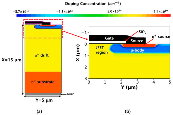
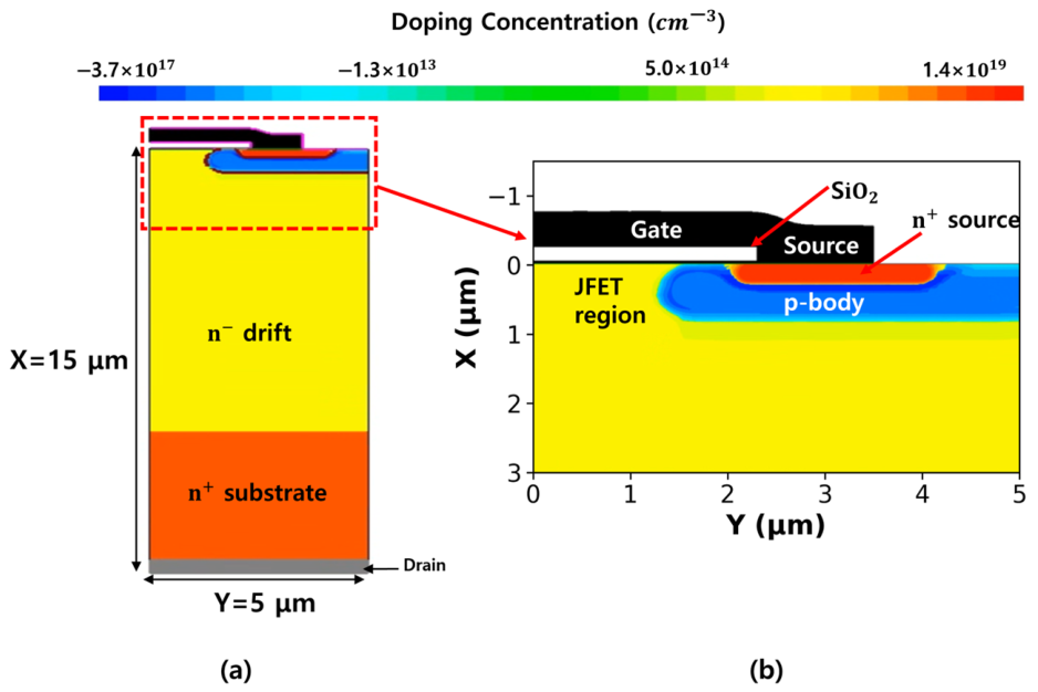
Figure 1 shows the TCAD simulation structure of a planar 4H-SiC n-channel MOSFET, modeled as a half-cell with a width of 5 μm. The n-type drift layer, 10 μm thick with a doping concentration of 5 × 1015 cm−3, lies on an n+ substrate (1 × 1019 cm−3); the n-type drift region in direct contact with the gate oxide surface constitutes the junction field-effect transistor (JFET) region. The lateral coordinate Y is defined with the center of the cell as the origin, and the depth coordinate X is defined with the SiC surface as the origin. As Y increases, the JFET region, channel, and n+ source appear. At the SiC surface, the JFET–p-body and p-body–n+ boundaries are located at Y = 1.56 and 1.85 μm, respectively, giving a surface channel length of 0.29 μm. The key device and trap parameters are summarized in Table 1.
Figure 1.
Structure and doping distribution of the simulated 4H-SiC MOSFET half-cell: (a) overall cross-section and (b) enlarged view of the gate region.
Table 1.
Key device and trap parameters.
The simulations were performed with the two-dimensional drift-diffusion method using Synopsys Sentaurus TCAD simulation [13]. Fermi–Dirac statistics were used for the carrier distribution [14]. The Shockley–Read–Hall model with doping and temperature dependence and the Auger model were applied for recombination. The mobility model included doping concentration dependence, high-field saturation, and mobility degradation due to the electric field normal to the interface. The mobility anisotropy according to the 4H-SiC crystal direction was also considered [15].
The lattice temperature was fixed at 300 K. Because a two-dimensional TCAD simulation calculates the current per 1 μm of device width, the half-cell current was multiplied by 5 × 10⁵. This accounts for the third dimension of the MOSFET and reproduces the current that an actual device would carry; it corresponds to 5 × 10⁵ half-cells connected in parallel. The ID–VGS transfer curves were obtained by sweeping VGS from 0 to 10 V at VDS = 10 V. Vth was determined using the constant-current method, defined as the VGS at which ID reaches the reference current Io = 1 mA [16]. gm was extracted as the maximum slope obtained by dividing the change in ID by the change in VGS between two adjacent points, and Ion is the drain current at VGS = VDS = 10 V. Vth could not be extracted using the constant-current method under conditions where ID did not reach 1 mA within the sweep range, so values extrapolated beyond the sweep range were not used as Vth.
2.2. DD Modeling and Dataset
The DDs were implemented as single-level acceptor-like traps in the SiC bulk. Because an acceptor-like trap is negatively charged when it captures an electron and neutral when it is empty, the traps in n-type regions where the Fermi level is above the trap level capture electrons, become negatively charged, and compensate donors [8,13]. The traps were placed uniformly with a concentration Nt within a range of ±σ in each direction from the center (X, Y). The portion extending outside the SiC surface was excluded. Therefore, σ is the half-width of the trap region, and the total number of traps depends on Nt and the actual size of the trap region inside the SiC. The energy level is the depth Ec−Et measured from the bottom of the conduction band. As shown in Table 2, simulations were performed for 5 × 8 × 8 × 7 × 5 = 11,200 conditions using a full-factorial combination of five energy levels, eight concentrations, eight depths, seven lateral positions, and five distribution widths. The depth X = (1–20) nm covers the near-interface region, and Y = (0.5–3.5) μm covers the JFET, channel, and n+ source regions. With the carrier removal rates reported for neutron irradiation (11–18 cm−1) [7,8], even the lowest Nt of 3 × 1016 cm−3 corresponds to a fluence six times higher than that which fully compensates the drift layer under uniform irradiation. Therefore, Nt represents the local defect concentration within a near-interface damaged region, such as the end-of-range region of light ions, rather than a device-average value [8].
Table 2.
Sweep variables of the technology computer-aided design (TCAD) simulation dataset.
Vth, gm, and Ion were extracted as outputs. The reference values, excluding the effect of the traps, are Vth = 2.894 V, gm = 20.78 S, and Ion = 45.86 A. The changes ΔVth, Δgm, and ΔIon are defined as the differences from these reference values under all conditions.
2.3. Device Degradation Characteristics Due to DDs
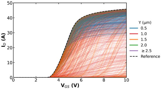
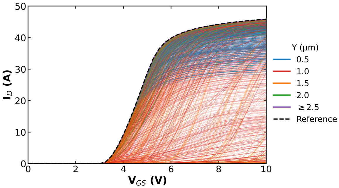
Figure 2 compares the ID–VGS curves for different lateral trap positions. At Y ≥ 2.5 μm, the difference between Ion and the reference value is less than 0.2%, so all curves overlap with the reference curve. At Y = 0.5 μm, the turn-on voltage remains unchanged, while the saturation current decreases to a minimum of 28 A. In contrast, at the JFET edge (Y = 1.0 μm) and the channel entrance (Y = 1.5 μm), the entire curve shifts toward higher VGS values, and under some conditions, the device does not turn on at all even at VGS = 10 V. The curve at Y = 2.0 μm lies just below the reference curve, indicating relatively small degradation at this position.
Figure 2.
Transfer characteristics (ID–VGS) for different lateral trap positions (Y). The dashed line indicates the reference curve.
Table 3 summarizes the maximum changes in Vth, gm, and Ion as all other variables were varied at each lateral position. At the JFET edge (Y = 1.0 μm) and at the channel entrance (Y = 1.5 μm), Vth increased by up to 7.09 V, while gm and Ion dropped to nearly zero. The JFET center (Y = 0.5 μm) exhibited different behavior. While Vth remained unchanged, Ion decreased by up to 38%. Traps in the n+ source region beneath the gate (Y = 2.0 μm) had a weaker effect, reducing gm and Ion by up to 31% and 11%, respectively. When the trap was outside the gate (Y ≥ 2.5 μm), none of the three output parameters changed by more than 0.5%.
Table 3.
Maximum degradation relative to the reference values at each lateral trap position Y, evaluated across all turned-on conditions.
At the same Y, the depth X had little effect as long as the trap region reached the interface (X ≤ σ), which held for 95% of the conditions. Only for σ = 10 nm and X = 15 and 20 nm was the trap region separated from the interface by 5 and 10 nm, respectively. In these cases, the degradation decreased sharply: at Y = 1.5 μm, 0.6 eV, and 3 × 1019 cm−3, the Ion reduction was 99.9%, 34.0%, and 0.9% at X = 10, 15, and 20 nm, respectively. Among the conditions with noticeable degradation, the median degradation fell to 49% and 11% of its contact value with gaps of 5 and 10 nm, respectively. Thus, the gap between the trap region and the interface, rather than the center depth, is decisive.
The degradation also increased with the distribution width at the same Nt. Because a wider distribution also contains more traps, conditions with similar total trap amounts (within a factor of 1.6) were compared. At the JFET center (Y = 0.5 μm), the degradation followed the total trap amount until it saturated, and the saturation level was set by σ (5.8% for σ = 10 nm and 27.7% for σ = 100 nm at X = 8 nm and 0.6 eV); the wider distribution degraded more in 96% of the matched pairs. At the channel entrance (Y = 1.5 μm), the narrower, more concentrated distribution degraded more in 95% of the pairs, because the inversion layer within a few nanometers of the interface responds to the local trap concentration.
The position dependence shown in Table 3 is related to the charge state of the acceptor-like traps. In the JFET region, since the Fermi level is above the trap level, the traps capture electrons and become negatively charged, compensate for the donors, and deplete the accumulation path beneath the gate. In a planar MOSFET, electrons that have passed through the channel flow into the drift region via the accumulation layer on the surface of the JFET region. Therefore, when the negative charge of the traps reduces the electron concentration in the accumulation layer, the current is suppressed. In particular, at the channel entrance, where the surface is weakly n-type owing to compensation between the p-well and drift doping, the negative charge of the traps converts this region into effectively p-type, extending the region that must be inverted and thus directly raising Vth. At the JFET edge (Y = 1.0 μm), the traps lie on the path through which electrons leaving the channel enter the JFET region; depleting this path keeps ID below Io up to a higher VGS, so the Vth extracted using the constant-current method increases even though the traps do not reach the channel.
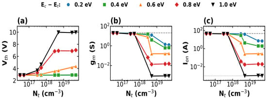
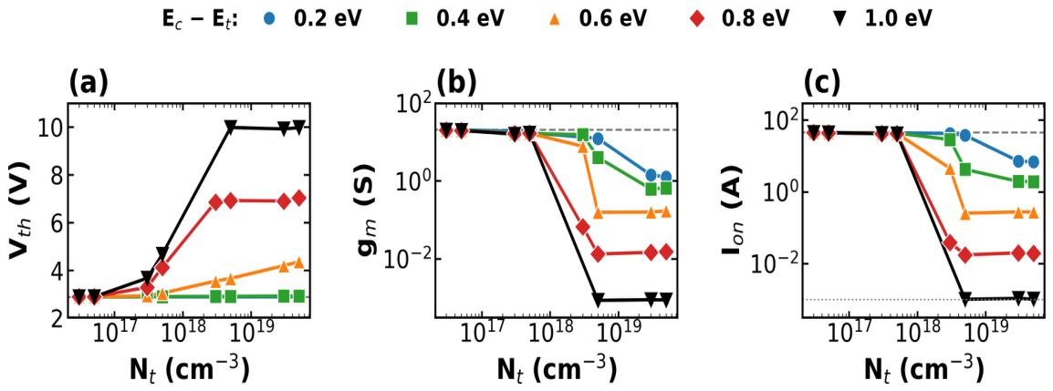
Figure 3 shows Vth, gm, and Ion according to the trap concentration and energy level at Y = 1.0 μm, X = 8 nm, and σ = 100 nm, among the most sensitive positions. Even at the lowest DD-induced trap concentration considered, 3 × 1016 cm−3, Ion decreased by 0.9–1.7%, and the degradation appeared continuously with concentration over the entire concentration range considered. At 3 × 10¹⁷–5 × 1017 cm−3, the Ion reduction was 2–10% and the Vth increase was within 1.8 V. At 3 × 1018 cm−3, levels of 0.4 eV or deeper turned into severe degradation, with Ion decreasing by 37–100%. At this position, Vth extracted at 1 mA increased by approximately 4 V at 0.8 eV and by approximately 7 V at 1.0 eV; whether this is an actual shift is examined below. The saturation concentration at which degradation ceased to increase was higher for shallower energy levels. Across the entire dataset, the concentration at which the maximum Ion reduction reached 100% was 3 × 1018 cm−3 at 0.8 eV or deeper, 5 × 1018 cm−3 at 0.6 eV, and 3 × 1019 cm−3 at (0.2–0.4) eV.
Figure 3.
(a) Vth, (b) gm and (c) Ion as a function of trap concentration Nt for different trap energy levels Ec−Et at Y = 1.0 μm, X = 8 nm, and σ = 100 nm. Dashed lines indicate the reference values, and the dotted line in (c) indicates the reference current Io = 1 mA.
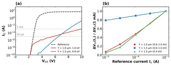
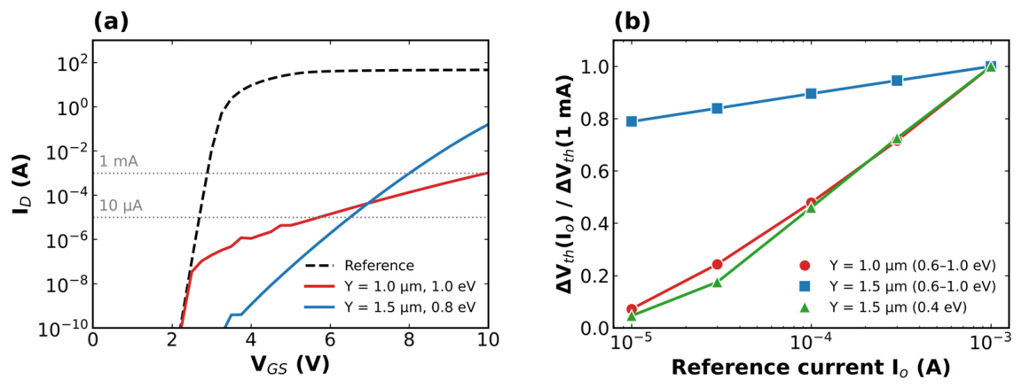
At the same concentration, ΔVth and ΔIon increase as the energy level deepens. At Y = 1.0 μm, shallow energy levels of 0.2 and 0.4 eV caused almost no change in Vth (less than 0.04 V), but Ion decreased to 6.9 and 1.9 A at 5 × 1019 cm−3, respectively. Shallow traps primarily capture electrons after turn-on, when the Fermi level approaches the conduction band; therefore, they affect Ion more than Vth. Deep traps carry a negative charge even before turn-on, causing Vth to shift. At 0.2 eV, Vth varied by no more than 0.1 V even at Y = 1.0 and 1.5 μm. Figure 4 shows Vth extracted at lower reference currents to distinguish an actual Vth shift from an apparent one caused by current suppression. At Y = 1.5 μm, the 0.4 eV level also raised the Vth extracted at 1 mA, but only 5% of this shift remained at 10 μA, indicating an apparent shift. An actual Vth shift, retaining 67–89% of its value at 10 μA, occurred only at 0.6 eV and deeper at Y = 1.5 μm. In contrast, at Y = 1.0 μm, only 7% (median) of the shift at 1 mA remained at 10 μA, confirming that the Vth increase at the JFET edge is an apparent shift caused by current suppression.
Figure 4.
(a) ID–VGS curves of the reference device and of devices with traps at Y = 1.0 μm (1.0 eV) and Y = 1.5 μm (0.8 eV). The dotted lines indicate ID = 1 mA and 10 μA. (b) Median ratio of ΔVth extracted at a reference current Io to that extracted at Io = 1 mA.
3. Data Preprocessing and DNN Model Design
3.1. Data Preprocessing
Because radiation reliability assessment determines how much the device characteristics change under specific defect conditions, the conditions with large degradation indicate the region where prediction is needed. However, in this region, the nonlinearity of the characteristics and the prediction error increase; thus, removing such conditions from the training data would improve the metrics but would not secure the predictive capability that is needed. Therefore, only numerically invalid results were removed via preprocessing, and the application range was limited to the conditions that turn on within the gate sweep range.
Table 4 shows the content of each step and the numbers of removed and remaining data. Method I removed 436 conditions that did not converge and did not complete the calculation up to VGS = 10 V. Method II covers 377 conditions in which the current decreased by 0.5 dec or more as the gate voltage increased after turn-on; a current decrease with increasing gate voltage cannot be explained physically and was therefore judged to be a numerical error and removed. Method III separated 86 conditions in which ID did not reach the reference current Io at VGS = 10 V. For these conditions, Vth cannot be extracted within the sweep range, and gm and Ion are also not post-turn-on characteristics; therefore, to keep the same application range for the three models, these conditions were excluded from all three models. Method IV involves only scaling the input and output values without removing any data, and applies the standardization method used in a study on neural network-based prediction of SiC device characteristics [17]. Since the ranges and units of the input variables differed, the trap concentration Nt and the distribution width σ were converted to common logarithms and then z-score standardized so each of the five inputs and outputs had zero mean and unit standard deviation to prevent variables with large magnitudes from dominating the learning process. If the trap concentration were standardized using its original linear scale, six out of eight concentrations (3 × 10¹⁶–5 × 10¹⁸) cm−3 would be concentrated in a narrow range from −0.63 to −0.35, and the difference around 3 × 1017 cm−3 would be virtually indistinguishable in the input. Therefore, a log transformation was used to even out the concentration intervals. Since Ion is distributed over five orders of magnitude—from 10−3 to 4.6 × 101 A—even within the valid range, was used, and the predicted values were inverse-transformed after training. The mean and standard deviation used for standardization were calculated only from the training set, and the same values were applied to the validation and test sets.
Table 4.
Data preprocessing steps.
Because the excluded conditions were not uniformly distributed, their effect on the application range was examined. The non-converged conditions (Method I) were spread over all variables; 427 of them had reached 1 mA before the calculation stopped, and the trained DNN predicted their Vth with an MAE of 0.003 V. Their exclusion therefore does not narrow the application range. In contrast, 433 of the 463 conditions removed or separated by Methods II and III were located at the channel entrance under high trap concentrations and deep levels, where the device barely turns on, so this region lies outside the range of the regression models. To identify such conditions, a classifier was trained on the 10,764 converged conditions to determine whether the device turns on within the sweep range, and it achieved an accuracy of 99.7% on the test set. Combined with this classifier, the regression models can be applied only to the conditions in which the device turns on.
3.2. DNN Configuration and Training
Since Vth, gm, and Ion are different physical quantities and exhibit different response patterns to concentration, they were trained using separate DNN models. All three models are fully connected neural networks that take five inputs and produce one output, and the hidden layers use the sigmoid linear unit (SiLU) activation function. We compared 16 combinations of hidden layer width (128, 256), depth (3, 4), learning rate (10−3, 5 × 10⁻⁴), and batch size (64, 128) based on validation loss. The selected architectures are shown in Table 5. The Adam optimizer and mean squared error (MSE) loss function were used. If the validation loss did not decrease for 40 epochs, the learning rate was halved. If it did not decrease for 120 epochs, training was terminated, and the weights with the minimum validation loss were adopted. The random seed used for data splitting, weight initialization, and mini-batch ordering was fixed at 42. PyTorch (version 2.15.0) was used for the implementation [18].
Table 5.
Selected deep neural network (DNN) architecture and hyperparameters.
The dataset was partitioned into training, validation, and test sets at a ratio of 70:15:15. For all three models, the entire dataset of 10,301 conditions was split into 7210/1545/1546 conditions, and the test set is common. The split was stratified by response (|ΔVth| ≥ 0.01 V, |Δgm| ≥ 0.1 S, or |ΔIon| ≥ 0.1% of the reference Ion) so that the proportion of responsive samples is the same in the three subsets.
For the N samples in the test set, yi is the TCAD simulation value, is the DNN prediction, and is the mean of all yi in Equations (1) and (2). MAE is the mean of the absolute prediction errors and has the same unit as the output, so it directly shows how large the errors are. However, if most of the data are clustered around the reference value, even a model that simply outputs the reference value will yield a small MAE. R2 represents the proportion of the test set’s variance explained by the model. It is 0 if the model outputs only the mean and 1 if it predicts perfectly, thus indicating how well the model tracks variations in the data. Since the two metrics are complementary, they are presented together. For the Vth and gm models, the metrics were calculated after converting the predicted values on the standardized scale back to their original units (V, S). For the Ion model, whose values span five orders of magnitude within the valid dataset, the metrics were calculated in the space. Since 57.6% of the test set did not meet the response criteria, the DNN’s performance metrics were calculated for the entire test set and the 656 test samples that met the response criteria.
4. Prediction Results and Discussion
4.1. Prediction for the Test Set
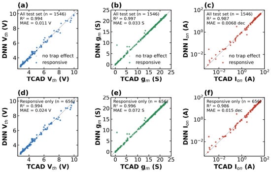
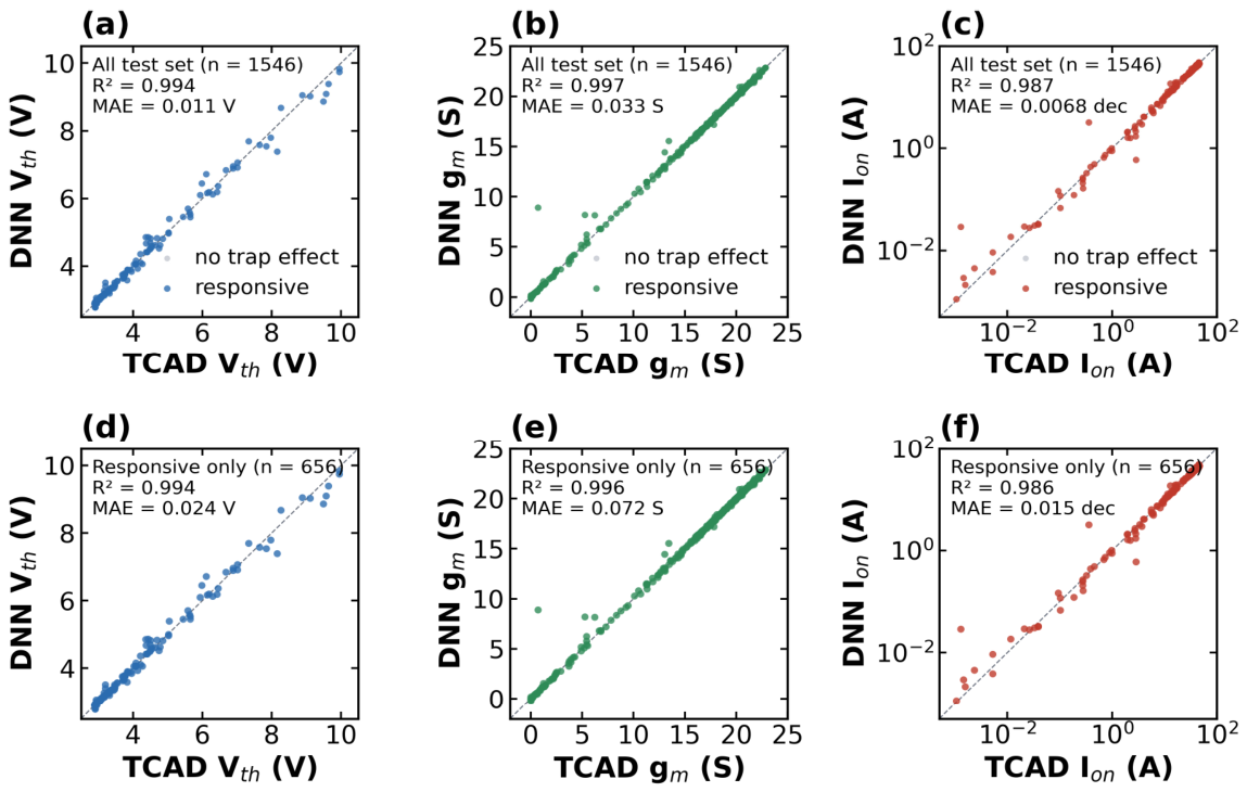
Figure 5 shows the parity plots of the three models trained with the architectures in Table 5 for the test set. Vth followed the diagonal over the entire range from the reference value of 2.89 to 9.9 V near the turn-on limit; 42 conditions had errors exceeding 0.1 V, 14 conditions had errors exceeding 0.3 V, and the maximum error was 0.77 V. gm was reproduced from the (22–23) S region, which is larger than the reference value, down to the 10−3 S level; however, 17 conditions had errors exceeding 0.3 S, such as a condition of 0.69 S predicted as 8.9 S, and negative values as low as −0.18 S were predicted for some conditions with gm close to 0. These predictions were clipped at 0. In additional tests, a softplus output layer eliminated negative predictions but increased the MAE from 0.038 to 0.051 S, and a log-scale target reduced the median relative error for gm < 1 S from 83% to 17% but increased the overall MAE to 0.157 S. The linear model with clipping was therefore retained; the log-target model is preferable when the relative accuracy of small gm matters. Ion was predicted over five orders of magnitude from the reference value of 46 A to 1 mA; four conditions had log errors exceeding 0.3 dec, and the maximum error was 1.35 dec.
Figure 5.
Parity plots of the Vth, gm, and Ion models for (a–c) the whole test set (n = 1546) and (d–f) the responsive samples only (n = 656). R2 and mean absolute error (MAE) are given in each panel. The dashed line indicates perfect agreement (x = y), and gray dots indicate samples without a trap effect.
For the entire test set, the Vth model achieved R2 = 0.994 and MAE = 0.011 V, the gm model achieved R2 = 0.997 and MAE = 0.033 S, and the Ion model achieved R2 = 0.987 and MAE = 0.0068 dec on the log scale. Even when evaluated only on the responsive samples, the R2 was 0.994, 0.996, and 0.986 and the MAE was 0.024 V, 0.072 S, and 0.015 dec, showing high prediction performance for the responsive samples as well.
Conditions with large errors mostly occurred in the severely degraded region where Y = (1.0–1.5) μm. Conditions with large Vth errors were primarily observed in the region where Y = 1.0 μm, X = (10–20) nm, σ = (80–100) nm, and Nt ≥ 5 × 1018 cm−3; this is the region where Vth rises sharply to (7–10) V. Large errors in gm and Ion were concentrated in the region where Y = 1.5 μm, σ = (10–20) nm, and X = (10–15) nm. Under these conditions, the half-width of the trap is similar to the center depth, so whether the trap region touches the interface depends on small differences in X and σ, resulting in a sharp change in output. These represent two types of abrupt transitions: the turn-on limit for Vth and the interface-contact boundary for gm and Ion. In an additional test, adding X–σ as a sixth input reduced the number of Ion errors exceeding 0.3 dec from 5 to 1 and halved the Ion MAE near the contact boundary, showing that the contact-boundary errors can be reduced by providing the gap to the interface explicitly. In contrast, the Vth errors near the turn-on limit were unchanged, indicating that this boundary requires denser sampling rather than a different input. Overall, the errors in the DNN are concentrated at the boundary where the output changes sharply with respect to the input, while in other regions, the DNN quantitatively reproduces the changes in the three characteristics.
4.2. Prediction for Unseen Conditions
Because the test set was randomly split from the same grid, the prediction of unseen parameter values was examined separately. First, when one intermediate level of a variable was excluded from training (Ec−Et = 0.6 eV, Nt = 5 × 10¹⁷ or 3 × 1018 cm−3, X = 6 nm, or σ = 50 nm), the Vth MAE was 0.007–0.047 V and the log10Ion MAE was 0.006–0.025 dec. However, the models failed when a lateral position (Y = 1.0 or 2.0 μm) was excluded, because the degradation changes discontinuously between the JFET, channel entrance, and source regions.
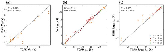
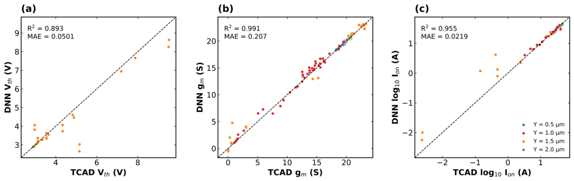
Second, 288 new TCAD conditions were simulated in which Ec−Et (0.3, 0.5, 0.7, and 0.9 eV), Nt (1017, 1018, and 1019 cm−3), X (3 and 12 nm), and σ (15, 30, and 65 nm) simultaneously took values not used in training, with Y kept at 0.5, 1.0, 1.5, and 2.0 μm. After the same preprocessing, 264 conditions remained. Figure 6 compares the DNN predictions with the TCAD results for these conditions. The DNNs achieved R2 values of 0.893, 0.991, and 0.955 and MAEs of 0.050 V, 0.21 S, and 0.022 dec for Vth, gm, and log10Ion, respectively. The Vth MAE was 0.006 V or less at Y = 0.5, 1.0, and 2.0 μm but 0.25 V at Y = 1.5 μm, where the errors arose between grid points at which the characteristics change abruptly.
Figure 6.
Parity plots of the DNN predictions for 264 new TCAD conditions with unseen parameter combinations: (a) Vth, (b) gm, and (c) log10Ion. Colors indicate the lateral position Y. The dashed line indicates perfect agreement (x = y).
Table 6 compares the DNN with multilinear grid interpolation, Gaussian process regression (GPR) [19], and random forest (RF) [20]. Grid interpolation could be applied to only 177 conditions (67%) because some of the 16 surrounding grid points had been excluded. On these common conditions, the DNN gave the lowest MAEs for all outputs. Over all 264 conditions, RF yielded R2 values of 0.34, 0.60, and 0.17, and GPR, trained on a 2000-sample subset with a radial basis function kernel, failed to predict between grid points. Within the original grid, RF was comparable to the DNN; the advantage of the DNN therefore lies in its stable prediction of unseen parameter combinations as a single continuous function. Within the training range and at the simulated lateral positions, the DNN can predict the degradation for various combinations of trap parameters without TCAD simulation.
Table 6.
Mean absolute error of each model on the 177 new conditions that all models could predict.
5. Conclusions
The DDs near the interface between the gate oxide and SiC in a 4H-SiC MOSFET were modeled as acceptor-like traps. TCAD simulations were performed using 11,200 conditions created by combining five parameters (energy level, concentration, depth, lateral position, and distribution width) and the resulting degradation of Vth, gm, and Ion was analyzed. When DDs were present near the interface, the factors influencing device degradation were their position, energy level, concentration, and whether they were in contact with the interface. First, the lateral position of the trap determined the degree of degradation, which was most severe at the channel entrance (Y = 1.5 μm) and at the JFET edge (Y = 1.0 μm). At the center of the JFET (Y = 0.5 μm), only Ion showed a reduction of up to 38% without any change in Vth, while there was almost no effect outside the gate. The degradation characteristics of the traps depending on their location can be explained by the fact that the negative charge of the electron-capturing traps hindered the formation of the inversion layer and the accumulation layer on the JFET surface. Shallow energy levels at 0.2 eV reduced Ion without shifting Vth, whereas an actual Vth shift occurred only at 0.6 eV and deeper, and the Vth increase at the JFET edge was an apparent shift caused by current suppression. The effect became apparent starting at the lowest concentration of 3 × 1016 cm−3 even at (0.2–0.4) eV, with higher saturation concentrations observed at shallower energy levels. The depth from the interface itself had little effect; rather, it was critical whether the trap region touched the interface. When the trap region spanned the interface, the difference depending on the depth (1–20) nm was small, and the effect of the distribution width depended on the position: a wider distribution degraded the JFET region more, whereas a narrower, more concentrated distribution degraded the channel entrance more.
These factors interact, so degradation cannot be captured with a simple equation or linear interpolation. A single TCAD run takes minutes to hours depending on the condition, and sweeping every combination of variables this way is not practical. Therefore, we preprocessed the 11,200 conditions, removing runs that did not converge, curves whose current fell non-physically after turn-on, and conditions in which the reference current was not reached within the sweep range. The DNNs were trained on the remaining 10,301 valid conditions. On the test set, they reached R2 = 0.994 (MAE = 0.011 V) for Vth, R2 = 0.997 (MAE = 0.033 S) for gm, and R2 = 0.987 (MAE = 0.0068 dec) for . Restricting the evaluation to the responsive samples, where the trap effect actually appeared, changed little: R2 values of 0.994, 0.996, and 0.986 with MAE values of 0.024 V, 0.072 S, and 0.015 dec were obtained. The largest errors occurred at boundaries where the output jumps with a small change in input; elsewhere, the DNN reproduces the three characteristics quantitatively. For 264 new conditions with unseen parameter combinations, the DNNs achieved R2 values of 0.893, 0.991, and 0.955 and outperformed grid interpolation, GPR, and RF. The trained DNNs thus predict the degradation for new combinations of trap parameters at the simulated lateral positions without a TCAD run. Radiation-induced degradation should be treated as a design constraint rather than verified only after the initial performance is secured. These predictions can be used to set design margins and test conditions for SiC power devices intended for radiation environments.
Author Contributions
Conceptualization, methodology, formal analysis, and writing—original draft preparation, G.P.; supervision and writing—review and editing, J.K. All authors have read and agreed to the published version of the manuscript.
Funding
This research was funded by the Korea Institute of Energy Technology Evaluation and Planning (KETEP) and the Ministry of Climate, Energy & Environment (MCEE) of the Republic of Korea (No. RS-2026-25538218) and by the KERI Primary Research Program of MSIT/NST (No. 26A01091).
Data Availability Statement
The data presented in this study are available on request from the corresponding author.
Acknowledgments
During the preparation of this manuscript, the authors used Claude (Opus 5.5, Anthropic, San Francisco, CA, USA) for the purposes of assisting with translation. The authors have reviewed and edited the output and take full responsibility for the content of this publication.
Conflicts of Interest
The authors declare no conflicts of interest.
Abbreviations
The following abbreviations are used in this manuscript:
| DDs | Displacement defects |
| DNN | Deep neural network |
| GPR | Gaussian process regression |
| JFET | Junction field-effect transistor |
| MAE | Mean absolute error |
| MOSFET | Metal-oxide-semiconductor field-effect transistor |
| MSE | Mean squared error |
| RF | Random forest |
| SiLU | Sigmoid linear unit |
| TCAD | Technology computer-aided design |
References
- Kimoto, T.; Cooper, J.A. Fundamentals of Silicon Carbide Technology: Growth, Characterization, Devices, and Applications; Wiley-IEEE Press: Singapore, 2014. [Google Scholar] [CrossRef] [Scilit]
- She, X.; Huang, A.Q.; Lucía, Ó.; Ozpineci, B. Review of Silicon Carbide Power Devices and Their Applications. IEEE Trans. Ind. Electron. 2017, 64, 8193–8205. [Google Scholar] [CrossRef] [Scilit]
- Lauenstein, J.-M.; Casey, M.C.; Ladbury, R.L.; Kim, H.S.; Phan, A.M.; Topper, A.D. Space Radiation Effects on SiC Power Device Reliability. In Proceedings of the 2021 IEEE International Reliability Physics Symposium (IRPS), Monterey, CA, USA, 21–25 March 2021; pp. 1–8. [Google Scholar] [CrossRef] [Scilit]
- Akturk, A.; McGarrity, J.M.; Wilkins, R.; Markowski, A.; Cusack, B. Space and Terrestrial Radiation Response of Silicon Carbide Power MOSFETs. In Proceedings of the 2017 IEEE Radiation Effects Data Workshop (REDW), New Orleans, LA, USA, 17–21 July 2017; pp. 1–5. [Google Scholar] [CrossRef] [Scilit]
- Wu, X.; Mori, T.; Liu, W. Thermoelectric Stability as a Design Constraint for Energy Conversion. Joule 2026, 10, 102421. [Google Scholar] [CrossRef] [Scilit]
- Srour, J.R.; Marshall, C.J.; Marshall, P.W. Review of Displacement Damage Effects in Silicon Devices. IEEE Trans. Nucl. Sci. 2003, 50, 653–670. [Google Scholar] [CrossRef] [Scilit]
- Hazdra, P.; Popelka, S. Radiation Resistance of Wide-Bandgap Semiconductor Power Transistors. Phys. Status Solidi A 2017, 214, 1600447. [Google Scholar] [CrossRef] [Scilit]
- Hazdra, P.; Popelka, S. Displacement Damage and Total Ionisation Dose Effects on 4H-SiC Power Devices. IET Power Electron. 2019, 12, 3910–3918. [Google Scholar] [CrossRef] [Scilit]
- Lee, G.; Ha, J.; Kim, K.; Bae, H.; Kim, C.-E.; Kim, J. Influence of Radiation-Induced Displacement Defect in 1.2 kV SiC Metal-Oxide-Semiconductor Field-Effect Transistors. Micromachines 2022, 13, 901. [Google Scholar] [CrossRef] [Scilit]
- Kobayashi, T.; Hachiken, K.; Hirai, H.; Sometani, M.; Okamoto, M.; Hara, M.; Watanabe, H. Controlled Trap Formation in SiC Metal–Oxide–Semiconductor Structures via Gate Bias Stress and Its Impact on the Performance of Metal–Oxide–Semiconductor Field-Effect Transistors. J. Appl. Phys. 2026, 140, 045706. [Google Scholar] [CrossRef] [Scilit]
- Kim, J.; Kim, S.J.; Han, J.-W.; Meyyappan, M. Machine Learning Approach for Prediction of Point Defect Effect in FinFET. IEEE Trans. Device Mater. Reliab. 2021, 21, 252–257. [Google Scholar] [CrossRef] [Scilit]
- Mehta, K.; Wong, H.-Y. Prediction of FinFET Current-Voltage and Capacitance-Voltage Curves Using Machine Learning with Autoencoder. IEEE Electron Device Lett. 2021, 42, 136–139. [Google Scholar] [CrossRef] [Scilit]
- Synopsys, version R-2020.09; Sentaurus Device User Guide; Synopsys, Inc.: Mountain View, CA, USA, 2020.
- Blakemore, J.S. Approximations for Fermi-Dirac Integrals, Especially the Function F_1/2(η) Used to Describe Electron Density in a Semiconductor. Solid-State Electron. 1982, 25, 1067–1076. [Google Scholar] [CrossRef] [Scilit]
- Hatakeyama, T.; Fukuda, K.; Okumura, H. Physical Models for SiC and Their Application to Device Simulations of SiC Insulated-Gate Bipolar Transistors. IEEE Trans. Electron Devices 2013, 60, 613–621. [Google Scholar] [CrossRef] [Scilit]
- Ortiz-Conde, A.; García Sánchez, F.J.; Liou, J.J.; Cerdeira, A.; Estrada, M.; Yue, Y. A Review of Recent MOSFET Threshold Voltage Extraction Methods. Microelectron. Reliab. 2002, 42, 583–596. [Google Scholar] [CrossRef] [Scilit]
- Niu, X.; Sang, L.; Duan, X.; Gu, S.; Zhao, P.; Zhu, T.; Xu, K.; He, Y.; Li, Z.; Zhang, J.; et al. SiC MOSFET with Integrated SBD Device Performance Prediction Method Based on Neural Network. Micromachines 2025, 16, 55. [Google Scholar] [CrossRef] [Scilit]
- Paszke, A.; Gross, S.; Massa, F.; Lerer, A.; Bradbury, J.; Chanan, G.; Killeen, T.; Lin, Z.; Gimelshein, N.; Antiga, L.; et al. PyTorch: An Imperative Style, High-Performance Deep Learning Library. In Proceedings of the 33rd Conference on Neural Information Processing Systems (NeurIPS 2019), Vancouver, BC, Canada, 8–14 December 2019; pp. 8024–8035. [Google Scholar]
- Rasmussen, C.E.; Williams, C.K.I. Gaussian Processes for Machine Learning; MIT Press: Cambridge, MA, USA, 2006. [Google Scholar]
- Breiman, L. Random Forests. Mach. Learn. 2001, 45, 5–32. [Google Scholar] [CrossRef] [Scilit]

Disclaimer/Publisher’s Note: The statements, opinions and data contained in all publications are solely those of the individual author(s) and contributor(s) and not of MDPI and/or the editor(s). MDPI and/or the editor(s) disclaim responsibility for any injury to people or property resulting from any ideas, methods, instructions or products referred to in the content. |
© 2026 by the authors. Licensee MDPI, Basel, Switzerland. This article is an open access article distributed under the terms and conditions of the Creative Commons Attribution (CC BY) license.