Solver Steps or Solver-Free Retraining? A Same-Board Latency–Energy–Quality Characterization of Flow-Matching Speech Enhancement on a Power-Constrained Embedded GPU

Abstract

Speech enhancement on edge and wearable devices operates under strict power budgets; generative enhancers buy quality through repeated on-device evaluations. On a Jetson Orin NX, we characterize solver truncation and solver-free retraining for a 65.59 M-parameter flow-matching enhancer. Same-board latency, energy, and quality measurements yield a decision rule comparing two quantities: $N^{*}$, the smallest step count PESQ-equivalent to the retrained model (±0.05), and $N_{\max }$, the largest a mode affords. $N^{*}$ = 4 for the reference on this two-speaker corpus; $N_{\max }$ (p95) is 5 at the unconstrained mode and 2 at every constrained mode. We keep the solver where affordable; otherwise, under the PESQ criterion, only retraining reaches that quality among the compared recipes. Power modes are not a performance axis; incremental energy varies across budgets (2218 vs. 2022 mJ/s); a 0.048 M reference at MAXN shows 16.3× lower sustained end-to-end RTF at approximately 1% of the energy, 0.208 PESQ lower, with no detectable SI-SDR difference. At one pass, retraining gains 0.173 PESQ but loses 0.75 dB SI-SDR. The procedure is specified, not validated beyond this configuration: re-measure $N_{\max }$ on the target board and $N^{*}$ after a model, criterion, distribution, or arithmetic change.

1. Introduction

Speech is one of the most prevalent audio-domain biosignals on wearable and remote devices. Voice-assisted communication, telehealth monitoring and hearables research all require on-device processing under a strict power budget, at power levels spanning microcontroller-class wearables up to gateway-class edge modules. What does such a model actually cost the hardware, and where is the boundary? Diffusion- and flow-based enhancers reach their quality by integrating a learned trajectory over several network evaluations, and a fast-moving line of work has driven reported input–output latencies from hundreds of milliseconds to the tens. Every one of those numbers, however, is measured on a desktop or laptop GPU; deployed on embedded hardware are compact discriminative models one to three orders of magnitude smaller [1,2,3]. To our knowledge (literature search current to August 2026), what a generative speech enhancer costs on a Jetson-class GPU has not been measured before (discriminative-model deployments exist; Section 2). This paper measures that intersection. We take FlowSE (Lee et al., ICASSP 2025) [4]. A contemporaneous model shares the FlowSE name [5]; throughout this paper, FlowSE denotes Lee et al. FlowSE is a conditional flow-matching [6] enhancer built on an NCSN++ [7] backbone; we take it together with a single-step discriminative variant of the same backbone, and characterize both on a Jetson Orin NX across the three axes a deployer actually controls, namely, the number of solver steps, the power budget, and the model family. Throughout, solver-free retraining denotes this discriminatively trained variant. All measurements are taken on one board, and every direct comparison uses a matched timing caliber. The paper’s three calibers, namely, per-file CUDA-event, sustained stream, and whole-function wall clock, are mutually incomparable and are labeled wherever they meet. All are offline, full-utterance quantities of a non-causal model; RTF < 1 per power mode is a necessary condition for real-time; causal architectures such as Stream.FM [8] and batch workloads lie outside these measurements (Section 6). The two options are not same-level peers. Truncation is an inference-time control on a released model, while retraining is a design-time recipe. We characterize both under one matched protocol rather than ranking them.

The main contributions of this work are threefold:

1.

We formulate a matched-caliber, same-board protocol that combines the quality-side break-even $N^{*}$ with the board-specific solver budget $N_{\max }$.

2.

We characterize latency, energy, p95 solver feasibility, cross-session drift, and measured runtime-optimization effects for a flow-matching enhancer across four Jetson Orin NX power modes.

3.

We retrain FlowSE’s NCSN++ backbone as a single-step, solver-free discriminative model using residual parameterization and zero-parameter energy-adaptive conditioning, with separate ablations of both components. Under the same-board protocol, we compare solver-free retraining with solver truncation and compact discriminative anchors. The comparison informs deployment choices across the tested quality criteria and power modes; it does not establish a single model-wide ranking.

2. Related Work

Generative speech enhancement (SE) is moving toward real time (off embedded hardware). Diffusion- and flow-based SE reverse a stochastic differential equation (SDE) or integrate an ordinary differential equation (ODE) at inference [6,7] and have historically required tens of network evaluations; recent work reduces this to a handful or to one, along two routes. The first is few-step and single-step generative modeling. StoRM pairs a discriminative predictor with a few-step diffusion corrector [9]; CRP systematically studies few-step diffusion enhancement [10]; Thunder- and mean-flow formulations [11,12,13] compress inference to a single step. The second is streaming. Diffusion Buffer reports 320–960 ms input–output latencies [14], and its follow-up reports 32–176 ms [15]; Stream.FM reports a frame-causal design with 32 ms algorithmic latency [8], and causal flow-matching speech restoration reports a 20 ms total latency at five solver evaluations [16]. A third route, distilling a multi-step teacher into a few-step student [17,18], keeps a generative training objective; like every retraining strategy, it changes the training side rather than the deployment arithmetic, and it is not measured in this paper. Flow-native one-step training removes the solver by construction rather than by truncating it or retraining discriminatively; mean-flow and related formulations [11,12,13] train the network to map prior to target in one evaluation. Our retrained variant is not in this family; it is a discriminative regressor on the same backbone. A same-board comparison of truncated solving against a flow-native one-step model of this backbone would isolate what the generative objective itself contributes at one evaluation, and is the natural next measurement; its device cost on this board is unknown. Every one of the reviewed results is measured on a non-embedded GPU (RTX 4080 Laptop [8,14], RTX 2080Ti [15], RTX 4090 [11,12], V100 [13]) or stated with no measurement hardware named (step or multiply-accumulate (MAC) counts, or algorithmic latency [9,10,16]), and none of the reviewed studies reports energy.

Embedded SE deployment is an established, discriminative literature. DeepFilterNet2 (2.306 M) reports RTF 0.42 on a Raspberry Pi 4 [3]; DEMUCS-Mobile targets phones via pruning and low-bit quantization [19]; Rusci et al. deploy a recurrent neural network (RNN) enhancer on a multi-core RISC-V microcontroller and report energy, measured on 22 nm prototype silicon [20]. Compact discriminative designs [2,21,22,23,24] are engineered for edge budgets. On Jetson-class GPUs specifically, deploying and benchmarking discriminative speech stacks is established practice (NVIDIA’s Riva speech-AI SDK [25], deep neural network (DNN) inference benchmarks on Jetson [26]), and GTCRN (one model, 0.024 M as published, 0.048 M as released) [1] is one such compact design, though GTCRN’s published RTF 0.07 is measured on a desktop i5-12400. On the benchmark side, dedicated discriminative systems [27,28] hold the top VoiceBank-DEMAND scores. We do not claim to improve on any of these, and the discriminative models that did reach Jetson cannot answer the question “what does the solver cost”.

Our protocol follows the established Jetson practice of tegrastats sampling with idle-baseline subtraction, with the nvpmodel power mode reported alongside every wattage figure; energy-aware edge inference is itself an active literature [29,30]. On Orin-class modules, GPU power cannot be separated from SoC power by design, so board-level ${\mathrm{VDD}}_{\mathrm{IN}}$ is the board-level quantity we report.

3. Can the Solver Be Removed? System Under Test and Its Quality Cost

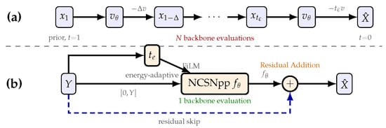
Both pathways (Figure 1) peak-normalize the noisy waveform y, compute its centered STFT S (510-point periodic Hann window; hop 128), and form $Y={0.15\left|S\right|}^{0.5}{e}^{\mathrm{j}\angle S}$. They use separately trained weights with the same 65.59 M-parameter NCSN++ parameter-name and tensor-shape schema; their inputs are $[x_t,Y]$ for the generative path and $[0,Y]$ for the retrained path. The generative path follows

$$x_t=(1-t)x_0+tY+{\sigma }_{t}z,{\sigma }_t=(1-t){\sigma }_{\min }+t{\sigma }_{\max },$$

(1)

where $x_0$ is the transformed clean spectrogram and z is standard complex Gaussian noise. The released checkpoint uses ${\sigma }_{\min }=0$ and ${\sigma }_{\max }=0.487$, giving the prior $x_1=Y+{\sigma }_{\max }z$. Conditional flow matching trains $v_{\theta }$ toward $Y-x_0+({\sigma }_{\max }-{\sigma }_{\min })z$. At inference, the released Euler sampler advances from $t_0=1$ to $t_N=0$ in N evaluations:

$$x_{t_{i+1}}=x_{t_i}-s_i{v}_{\theta }([x_{t_i},Y],t_i),s_i=t_i-t_{i+1}.$$

(2)

Figure 1. Spectral-domain inference. (a) Truncated FlowSE starts from $x_1=Y+{\sigma }_{\max }z$ and evaluates $v_{\theta }([x_t,Y],t_i)$ N times, with regular steps of size Δ and a final step of size $t_{\epsilon }$—Equation (2). (b) The retrained model maps $[0,Y]$ to one residual correction conditioned on $t_e$—Equation (3). The paths share the backbone architecture but use separately trained weights.

For $N\ge 2$, the first $N-1$ updates use $s_i=\Delta =(1-t_{\epsilon })/(N-1)$ and the final update uses $s_i=t_{\epsilon }=0.03$; for $N=1$, the single update uses $s_0=1$. Thus, N is the number of network evaluations. The retrained path removes the solver and predicts one deterministic residual [31],

$$\widehat{X}=Y+f_{\theta }\left([0,Y],t_e\right).$$

(3)

Here, $\widehat{X}$ is in the transformed spectral domain; the inverse transform and iSTFT produce $\widehat{x}$. An utterance-level, zero-parameter energy-adaptive scalar $t_e$, obtained by applying a clipped sigmoid to the log mean magnitude of Y, conditions the backbone’s existing time embedding; without energy conditioning, $t_e=1$.

Discriminative training of NCSN++ for speech enhancement follows Lemercier et al. (2023) [32], whose experiments used WSJ0-based datasets. We apply that recipe family to FlowSE’s backbone on VoiceBank-DEMAND [33]; Table 1 gives the residual and energy-conditioning ablations. We use the standard split, with 11,572 training utterances from 28 speakers and 824 test utterances from the 2 held-out test speakers. Every retrained configuration (M1, M2, M3, cold, warm) trains and selects on training-side material only; the warm initialization is FlowSE’s released checkpoint, trained by the original authors under their published setup [4]. Checkpoint selection uses validation PESQ on a 200-file validation subset; no test material enters training or selection. All variants are trained and evaluated by us on the same backbone and dataset; because objective and solver use both differ, the comparisons are recipe-level and make no solver-only mechanistic attribution. Each training configuration (M1, M2, M3, and the initialization variants in Section 4.2) is represented by one training run; all paired tests and intervals below quantify variation across the fixed test utterances conditional on the resulting checkpoints. Training-seed variability is measured for the warm single-stage recipe and for the reference’s multi-stage training chain, restricted to its last three stages from a shared parent checkpoint. The three warm data-order seeds span PESQ 3.013–3.049, SI-SDR 19.06–19.36 dB and ESTOI 0.875–0.877; the two chain seeds span PESQ 3.022–3.032, SI-SDR 18.84–18.87 dB and ESTOI 0.871–0.872. Each of the five replicates, taken as the equivalence anchor, gives $N^{*}$ = 3, where the original M3 anchor gives 4.

Table 1. Discriminative recipe-family ablation (VoiceBank-DEMAND, 824 utterances, raw weights). M1 = without energy-adaptive conditioning; M2 = without residual parameterization; M3 = full configuration (our single-step model). NFE = number of function evaluations (solver steps).

Configuration	PESQ	SI-SDR	ESTOI	CSIG	CBAK	COVL
M1 (no EA)	2.9972	18.373	0.8683	3.464	3.982	3.152
M2 (no residual)	2.7404	16.094	0.8450	3.397	3.940	3.077
M3 (full, ours)	3.0622	18.789	0.8711	3.470	4.004	3.169

All audio is 16 kHz. Training followed the original recipe of Adam with cosine scheduling and 5-epoch warmup (lr ${10}^{-4}$ in the main stages, ${10}^{-5}$ in the reference’s final fine-tuning stage), effective batch 32 via 8 × 4 accumulation, and an exponential moving average (EMA) of 0.999 with loss weights 0.5 complex-spectral/0.15 multi-resolution STFT [34]/0.5 SI-SDR (the last cosine-annealed out to zero over the first 30 epochs). Quality metrics are computed per file. We use PESQ in wideband mode [35,36], SI-SDR [37], ESTOI [38], DNSMOS [39] with a P.808-trained predictor [40]; the composite measures CSIG/CBAK/COVL in Table 1 follow Hu and Loizou [41].

Paired over 824 utterances with two-sided paired t-tests and Wilcoxon tests at scipy defaults, zero-differences dropped, exact and asymptotic modes automatic, and continuity correction off. In the tested realizations, the residual parameterization dominates, M3 over M2 by +0.322 PESQ (p = 1.3 × ${10}^{-176}$); the EA gain is small but statistically real in the tested realizations, M3 over M1 by +0.065 PESQ (p = 7.2 × ${10}^{-18}$).

Table 2 places M3 alongside the generative side over all 824 test utterances with raw weights. FlowSE rows are means over three sampling seeds and M3 is deterministic.

Table 2. Single-step retrained recipe versus solver truncation (VoiceBank-DEMAND, 824 utterances, raw weights). FlowSE rows are means over 3 sampling seeds; the single-step model is deterministic; differences quoted in the text use unrounded file-level values.

Configuration	NFE	PESQ	SI-SDR	ESTOI
FlowSE (5-step reference)	5	3.0919	18.845	0.8736
FlowSE truncated	1	2.8890	19.544	0.8735
M3 single-step (ours)	1	3.0622	18.789	0.8711

FlowSE draws its prior stochastically, so we run three sampling seeds and report the mean. M3 is deterministic; same-machine reruns are bit-identical, and the maximum difference between A100 and Orin outputs on 20 files is 3.34 × ${10}^{-4}$, consistent with floating-point variation. All paired statistics use the same three-seed filename means as the tables. Against the five-step reference, M3’s PESQ is lower by 0.030 with paired p = 3.2 × ${10}^{-3}$, a small but significant gap, while FlowSE retains a small SI-SDR edge of +0.056 dB at p = 0.068. Against truncated one-step FlowSE, M3 is higher by 0.173 PESQ, which is the quality difference between retraining and truncating at one forward pass.

Zero-state channels are not load-bearing. With $x_t$≡ 0 in M3, slicing those input channels leaves per-file metrics identical at four decimals across all 824 files (fp32, same checkpoint).

The 824 test utterances come from two speakers: 393 from p232 and 431 from p257. This large utterance count does not compensate for only two speaker clusters; one-step FlowSE trails M3 in PESQ by 0.1343 for p232 and 0.2088 for p257. Section 5 therefore broadens the speaker base to 20 VCTK speakers held out from the VoiceBank–DEMAND training and test sets. Across these clusters, M3’s mean PESQ is higher than FlowSE’s at every tested solver budget ($N=1$–5), supporting the PESQ competitiveness of single-pass, solver-free retraining. SI-SDR favors FlowSE and ESTOI is equivalent throughout, leaving the ranking criterion-dependent.

At Equal Device Cost, the Answer Depends on the Quality Criterion

At one forward pass, PESQ favors M3 by a wide margin, but that result does not generalize across criteria. Table 3 gives all seven metrics we can compute (PESQ [35], SI-SDR [37], ESTOI [38], DNSMOS [39], and a P.808-trained predictor [40]). Each utterance is enhanced once by each model and the scores are paired per file; the 90% confidence interval is the TOST-equivalent interval (two one-sided tests) used throughout. The FlowSE side is averaged over three seeds. The margins are ±0.05 PESQ, ±0.5 dB SI-SDR and ±0.01 ESTOI, fixed before the solver-step curve was measured and reported as post hoc; DNSMOS and P.808 carry no margin, so we report intervals only. No standardized smallest perceptually meaningful difference exists for PESQ; the ±0.05 margin sits at half of the instrument’s own single-condition accuracy (on the order of 0.1 MOS in the P.862 validation setting [42]), and no verdict depends on the choice ($N^{*}\in \{3,4\}$ for $\delta \in [0.03,0.08]$, Section 5). PESQ is the primary decision metric.

Table 3. Seven-metric comparison at one forward pass of FlowSE (N = 1) minus M3 (ours), paired per utterance over 824 files; positive means FlowSE is better; the 90% CI is the confidence interval of the difference; relative changes are expressed against the M3 value of each metric; differences are computed from unrounded file-level values (e.g., 3.0622 − 2.8890 displays as 0.173).

Metric	FlowSE N = 1	M3	Δ (FlowSE − Ours)	Relative	90% CI
PESQ	2.8890	3.0622	−0.1733	5.66%	[−0.1911, −0.1555]
DNSMOS SIG	3.4614	3.4705	−0.0090	0.26%	[−0.0138, −0.0043]
SI-SDR	19.5438	18.7894	+0.7544	4.02%	[+0.7106, +0.7982]
DNSMOS BAK	4.0614	4.0043	+0.0571	1.43%	[+0.0519, +0.0622]
DNSMOS OVRL	3.1930	3.1692	+0.0238	0.75%	[+0.0182, +0.0294]
P.808 MOS (predicted)	3.5876	3.5203	+0.0673	1.91%	[+0.0619, +0.0727]
ESTOI	0.8735	0.8711	+0.0024	0.28%	[+0.0012, +0.0037]

Table 3 shows that the two metrics favoring M3 (PESQ, DNSMOS-SIG) both quantify perceptual speech quality and cross over at the same N, one finding read twice, with magnitudes 5.66% and a negligible 0.26%. Of the remaining five, four favor FlowSE (waveform fidelity, background suppression, and the two overall-MOS predictors, DNSMOS OVRL and P.808) and are likewise not four independent losses; the fifth, ESTOI, measures intelligibility, and the two models are operationally equivalent on it at every N tested (below). At one forward pass, the retrained recipe improves PESQ by 5.66% while changing DNSMOS-SIG by only 0.26%, costs 0.75 dB of waveform fidelity, and is operationally equivalent in intelligibility (ESTOI inside the ±0.01 operational margin while significantly favoring FlowSE, p = 9.6 × ${10}^{-4}$). Which of those a deployer should care about is a property of the application, not of the models. No multiplicity correction is applied; every difference we call significant survives a Bonferroni adjustment by seven (the borderline case is the ESTOI value above, 6.7 × ${10}^{-3}$ after adjustment). The PESQ step scan that defines $N^{*}$ is a monotone threshold estimation rather than a family of tests (all five per-N intervals are reported below), and PESQ’s primacy follows VoiceBank-DEMAND benchmark convention rather than a post hoc choice among the seven metrics.

This sharpens the break-even point in Section 5. $N^{*}$ is metric-dependent; perceptual metrics saturate at different step counts, as established for this model family [43,44]; the latter reports WER moving with step count far more than PESQ does. WER lies outside our metric set, and we make no claim about it. On PESQ, FlowSE needs four solver steps to become statistically equivalent ($N_{\mathrm{equiv}}^{*}=4$) and five to become significantly better ($N_{\sup }^{*}=5$). At N = 3 the FlowSE − M3 difference is −0.0400 with 90% CI [−0.0579, −0.0221], crossing the −0.05 bound; at N = 4, it is +0.0086 with CI [−0.0086, +0.0259], inside. The one-sided tests (df = 823) give at N = 3 t₁ = +0.92 (p₁ = 0.179, failing to reject $\mu$ ≤ −0.05) and t₂ = −8.276 (p₂ = 2.6 × ${10}^{-16}$); at N = 4, t₁ = +5.58 (p₁ = 1.6 × ${10}^{-8}$) and t₂ = −3.94 (p₂ = 4.5 × ${10}^{-5}$), both p < 0.05, dual to the 90% CI. The remaining per-N intervals are N = 1 at −0.1733 [−0.1911, −0.1555], N = 2 at −0.1390 [−0.1574, −0.1207], and N = 5 at +0.0297 [+0.0131, +0.0462]. Per sampling seed the N = 4 interval stays inside ±0.05 (CI90 [−0.0094, +0.0259], [−0.0147, +0.0225], [−0.0050, +0.0325]) and N = 3 crosses the bound; pairing N = 4 against N = 5 within each seed gives −0.016 to −0.025 (upper bounds ≤−0.009). Two post hoc checks (descriptive, not cluster-corrected) bound this boundary. Within each speaker, the N = 4 interval stays inside the bound while the minimum operationally equivalent N splits (3 for p232, 4 for p257; noise-condition labels are not distributed with the test set), and anchoring on any of the five retrained realizations (three warm single-stage, two chain-segment replicates) gives $N^{*}$ = 3 for all five (between-seed spread 0.036 warm, 0.0103 chain). The original reference anchor scores above every replicate; the gap is systematic (same direction, similar size across both chain replicates) and larger than the measured seed spreads, and its source among environment, parent-checkpoint and recipe-deviation differences cannot be separated with two replicates. $N^{*}$ therefore takes 3 or 4 across speakers and anchors, and every mode-level decision is unchanged ($N_{\max }$ is 5 at the unconstrained mode and 2 at every constrained one). The intervals quantify across-utterance variation; inference-seed variation is shown per seed, speaker stratification above, and training-realization variation is reported in Section 3. SI-SDR reverses the PESQ ordering. At N = 1, FlowSE is already 0.7544 dB above the original M3 reference, with a 90% CI of [+0.711, +0.798]. The gap enters the ±0.5 dB equivalence band at N = 4 for the original reference and both chain anchors, at N = 3 for the original warm run, and at N = 1 for the two warm replicas. For ESTOI, the N = 1 difference is only +0.0024, with a 90% CI of [+0.0012, +0.0037], and every tested N and anchor lies within the ±0.01 band. Thus, $N^{*}$ depends on the criterion and reference anchor. Without a metric label, $N^{*}$ denotes the PESQ result throughout; single-metric optimization is a documented failure mode in this field [45].

4. Experimental Results

4.1. Where Does the Quality Go? An Exploratory Band-Wise Test of Over-Smoothing

The intuitive explanation for the perceptual deficit of truncated one-step FlowSE is over-smoothing, the classic failure mode of regression-trained enhancers [46]. One-step FlowSE sits 0.20 PESQ below its five-step counterpart, while the retrained model’s corresponding deficit is 0.03. We treat this as an exploratory diagnostic.

Table 4 shows that the L2-optimal configuration is two solver steps. N = 2 attains the lowest full-band complex-spectrum L2 error and the highest SI-SDR simultaneously. The L2 margin is ΔL2 = 1.81 ×${10}^{-4}$, ≈ 49× the seed standard deviation; the seed deviation itself is estimated from only three seeds, so the multiplier is imprecise though the margin is not. The SI-SDR margin is +0.093 dB (p = 8.8 × ${10}^{-111}$, paired over 824 files), and the two L2-type criteria agree here, though not by an exact identity. Nevertheless, N = 2 ranks second-worst of the five in PESQ. From N = 2 onward, the L2 error rises monotonically while PESQ rises with it, and M3 sits at the highest L2 error of all six configurations while placing third in PESQ. L2 optimality and perceptual quality therefore diverge systematically. Over-smoothing, as indexed by the tested proxies, does not explain the single-step perceptual deficit.

Table 4. PESQ, SI-SDR and full-band complex-spectrum mean-squared error (MSE) across solver-step counts (mean over 3 seeds; the single-step model is deterministic).

Configuration	PESQ (3-Seed Mean)	SI-SDR	Full-Band Complex-Spectrum MSE
FlowSE truncated (N = 1)	2.8890	19.544	0.013952
FlowSE (N = 2)	2.9232	19.637	0.013771
FlowSE (N = 3)	3.0222	19.355	0.014520
FlowSE (N = 4)	3.0709	19.062	0.015419
FlowSE (N = 5)	3.0919	18.845	0.016136
M3 single-step (ours)	3.0622	18.789	0.016846

The band-resolved statistics in Table 5 do not form a consistent over-smoothing story. Their magnitudes link to Table 4 by construction. The full-band column there is the bin-count-weighted average of these three bands (32, 96 and 128 frequency bins), over three seeds rather than the single realization here. On high-frequency energy retention, the ordering runs against the perceptual deficit. N = 1, the perceptually worst configuration in Table 4, preserves the most high-frequency energy (0.9909 versus 0.9815 at N = 5) and has the lowest error in every band. Spectral flatness does show the expected signature along the truncation direction (N = 1 flatter than N = 5), but it breaks down exactly where the hypothesis needs it most, because our M3, third-best in PESQ, is the flattest configuration of all (0.2156), with the least high-frequency retention (0.9722). The two band indicators therefore disagree with each other, and neither tracks PESQ. Over-smoothing, as indexed by these statistics, is not supported as the mechanism separating these systems; representation-level mechanisms outside these proxies are not excluded. SI-SDR and PESQ also rank the configurations oppositely here, the best waveform-domain configuration being among the worst perceptually and vice versa, so a deployer should select by a joint, application-specific criterion rather than by SI-SDR alone.

Table 5. Band-resolved complex-spectrum MSE, high-frequency (4–8 kHz) energy retention, and spectral flatness (higher = smoother) for three representative configurations (single realization per configuration, all 824 utterances; N = 1/N = 5 use the released FlowSE weights, M3 raw weights).

Configuration	cplx-MSE Low (0–1 kHz)	cplx-MSE Mid (1–4 kHz)	cplx-MSE High (4–8 kHz)	HF Energy Retention	Spectral Flatness
FlowSE truncated (N = 1)	0.10427	0.002156	2.453 × ${10}^{-4}$	0.9909	0.1690
FlowSE (N = 5)	0.12134	0.002364	2.652 × ${10}^{-4}$	0.9815	0.1575
M3 single-step (ours)	0.12592	0.002586	2.728 × ${10}^{-4}$	0.9722	0.2156

4.2. Must One Train from Scratch? An Initialization Ablation

All configurations here are evaluated on the 824 test utterances with raw weights (no EMA). Cold and warm are single 40-epoch runs of one discriminative recipe, Adam (lr 2 × ${10}^{-4}$, cosine over 40 epochs), effective batch 32, EMA 0.999, loss weights 0.5 complex/0.15 multi-resolution STFT/0.5 SI-SDR cosine-annealed out over the first 30 epochs, and differ only in initialization, random versus the released FlowSE checkpoint, with stored hyperparameters identical. The reference is the main model M3 in Table 1 and Table 2.

Table 6 gives two findings. In the tested single-run realizations, under the shared single-stage recipe, the initialization is decisive (ΔPESQ = +0.757, t = 62.1; SI-SDR and ESTOI likewise), while warm single-stage is statistically equivalent to the multi-stage reference (paired TOST against ±0.05 PESQ/±0.5 dB SI-SDR/±0.01 ESTOI, p = 1.2 × ${10}^{-6}$, 3.8 × ${10}^{-20}$, 1.1 × ${10}^{-12}$). Warm retains a very small PESQ deficit (Δ = −0.013), rank-detectable only (paired t-test, p = 0.090; Wilcoxon p = 4.5 × ${10}^{-4}$; no primary test was pre-specified; the disagreement suggests a skewed paired-difference distribution), and is significantly better on SI-SDR (+0.267, p = 4.5 × ${10}^{-25}$) and ESTOI (+0.006, p = 9.5 × ${10}^{-19}$); in the tested realizations, one warm-started run therefore substitutes the staged schedule, trading a sliver of PESQ for waveform- and intelligibility-domain gains. The equivalence margins were fixed for this study before the solver-step curve was measured, not pre-registered at the project outset, and equivalence holds for any margin exceeding 0.026 PESQ, 0.308 dB SI-SDR and 0.0066 ESTOI, the smallest bounds the data admit; the FlowSE initialization comes from the same dataset and task (same-task reuse, not cross-domain transfer), so the practical consequence is one training stage instead of a staged schedule.

Table 6. Initialization ablation (824 utterances, raw weights).

Config	Training	Init	PESQ	SI-SDR	ESTOI
cold	single-stage	random	2.2921	17.833	0.8200
warm	single-stage	FlowSE weights	3.0491	19.056	0.8767
reference	multi-stage	random	3.0622	18.789	0.8711

4.3. What Breaks on the Device?

4.3.1. Same-Board Latency and Energy Across Power Modes

The measurement protocol times latency per file with CUDA events over the network forward pass plus inverse STFT, with the input complex spectrogram Y precomputed and resident on the device (all preprocessing outside the timing window); forward-only reports are not comparable to ours. Two further calibers, sustained-stream (Section 4.3.4) and whole-function wall-clock (chunking, Section 4.3.3), are defined at their first uses and are not comparable with this one. Each (file, N) cell is a single pass at batch = 1. Warm-up was performed before every timed loop and excluded from the timed samples; the flow model used three utterances and the single-step model three utterances plus a 60 s sustained loop. Warm-up iterations were not retained, so Section 4.3.3’s first-file analysis concerns the first retained file, not cold start. Computation is fp32 with TF32 enabled for cuDNN convolutions but disabled for matmul. The board runs JetPack R36.4.7 with torch 2.11.0 and CUDA 12.6, 16 GB unified memory. Energy integrates on-module power from the power-monitoring chip INA3221 (tegrastats, 100 ms sampling, board-level ${\mathrm{VDD}}_{\mathrm{IN}}$) over the same utterance stream, with a measured idle baseline subtracted (cold 120 s/hot 60 s), giving the incremental energy per second of audio. This quantity is the sum over the stream of per-utterance energies $(P_i-P_{\mathrm{idle}})·{\mathrm{lat}}_i$, where $P_i$ is the power window over utterance i’s execution and ${\mathrm{lat}}_i$ is its latency, all divided by the total audio seconds. The product form $(P_{\mathrm{load}}-P_{\mathrm{idle}})·\mathrm{RTF}$ holds exactly only for the ratio-of-sums RTF; the per-file mean RTF used elsewhere differs from it by 1.8–2.2% on these runs, and the two are never interchanged. No external-meter cross-validation was performed. At the 100 ms telemetry rate, a mean-duration utterance yields only ~4 power samples at MAXN and ~9 at the constrained modes; the power window covers the ~0.4–0.9 s execution time rather than the 2.51 s audio duration; headline energies are therefore aggregated over the full utterance stream rather than reported per utterance, and idle-baseline drift is propagated separately into the energy-band uncertainty. Two internal checks bound repeatability rather than absolute accuracy. Per-utterance and sustained calculations from the same telemetry agree within 0.15–0.2%, and cross-session repeats spread by 0.17–1.33% in single-step energy. The INA3221 datasheet specifies a maximum gain error of 0.25% and a maximum offset of ±80 μV, but these specifications characterize only the monitor IC, not the complete measurement chain. A later verification session re-ran three configurations on the same day and showed a ≈0.3 W board-level shift relative to the initial measurement campaign. Its relative effect was −2.5% for the high-increment single-step model but −12% to −18% for GTCRN; consequently, ratios with small incremental-power denominators are reported only from interleaved same-session adjacent blocks. As a conservative uncertainty view, RTF varies by 0.6–3.8% across clean sessions and run protocols, while single-step energy varies by 0.17–1.33% across sessions (three MAXN values, pairwise 2218.3/2214.5/2189.2 mJ/s), exceeding any within-run telemetry dispersion. The n = 100 sweep subset is duration-stratified and calibrated against the full-824 N = 1 RTF mean within 1%. All device measurements use a single Orin NX module and the VoiceBank–DEMAND corpus. Of the two registered predictions, the step-budget prediction preceded all sweeps (Section 4.3.3); the constant-energy prediction’s anchor was finalized after the constrained-mode measurements and is analyzed as a post hoc band.

Across clean sessions and protocols, absolute single-step RTF varies by 0.6%–3.8%. Alternating the two models within one session versus running each in its own block gives MAXN values 0.16341 vs. 0.16246, a 0.6% spread, and 25 W values 0.33312 vs. 0.32058, 3.8%; the alternating arrangement exists to cancel session drift. Within a single session, paired same-run ratios agree to ≤0.1%. Deployment-relevant comparisons are therefore drawn from same-session paired measurements. Table 7 reports the per-mode single-step values; Table 8 tests the incremental energies against a constant-energy band.

Table 7. Same-board single-step latency and energy across power modes (single-step = the retrained model M3; energy in millijoules per second of audio, mJ/s). RTF and $E_{\mathrm{incr}}$ from the same session family (the block-design sweeps, the runs that also produce the $N_{\max }$ curves of Section 4.3.3); interleaved values appear only in the cross-session comparison above.

Mode	GPU Clock (MHz)	Cores	RTF Mean (Per-File)	RTF p95	Energy (mJ/s Audio)
MAXN	917	8	0.16246	0.18970	2218.3
25W	407	8	0.32058	0.37063	2107.4
15W	611	4	0.35727	0.41227	2115.7
10W	611	4	0.36216	0.41878	2022.2

Table 8. Incremental energy against the ±5% constant-energy band (final anchor = MAXN 2218.32 mJ/s, full-824 caliber; band [2107.40, 2329.24]), with idle-drift uncertainty. The ±5% width and the prediction were registered before the constrained-mode sweeps; the numeric anchor was finalized after the constrained-mode measurements, so the final band is a post hoc analysis band. Verdicts are reported under both this and the as-registered band.

Mode	${\mathit{E}}_{\mathbf{incr}}$ (mJ/s)	Deviation from Anchor	Idle Uncertainty
MAXN	2218.32	0% (anchor)	—
25W	2107.36	−5.002%	±1.11%
15W	2115.70	−4.626%	±2.4%
10W	2022.19	−8.841%	±2.5%

Because $E_{\mathrm{incr}}=(P_{\mathrm{load}}-P_{\mathrm{idle}})·\mathrm{RTF}$, a mode that runs proportionally slower at proportionally lower incremental power would pay the same energy per audio second. This is the constant-energy prediction that a constrained mode’s incremental energy per audio second stays within ±5% of the single-step MAXN anchor. It was registered before the constrained sweeps, but its centre moved twice as the anchor’s caliber was unified, the final 2218.32 mJ/s full-824 value being set after the 15 W and 10 W measurements and before the 25 W sweep. We therefore analyze the final band as post hoc. The verdict is anchor-sensitive at 25 W and 15 W and robust only at 10 W. Under the band as registered at measurement time (2254.04 ± 5%, i.e., [2141.34, 2366.74]), all three constrained modes sit below the lower edge, by 33.98 mJ/s (−1.51% of the anchor) at 25 W, 25.64 (−1.14%) at 15 W and 119.15 (−5.29%) at 10 W; under the final caliber-matched band, 15 W falls inside (−4.63%), 25 W sits on the edge (−5.00%, 0.04 mJ outside, too close to call against a ±1.11% idle-drift uncertainty, so we declare it indeterminate) and 10 W stays outside (−8.84%). We keep the final band as primary because it is the only comparison in which anchor and constrained values share the full-824 caliber, and we report the as-registered verdicts alongside it.

4.3.2. Cross-Mode Performance Cannot Be Extrapolated from GPU Frequency

The four power modes do not form a performance total order. The 25 W mode spends its budget on 8 CPU cores and runs its GPU slower than the 15 W mode (407 vs. 611 MHz); the 15 W mode runs a 1.50× faster GPU clock yet is about 11% slower (0.35727 vs. 0.32058, same caliber family). A mode change alters cores, CPU, GPU and external-memory-controller (EMC) clocks together. Table 9 quantifies the consequence. Neither frequency-only nor frequency-plus-cores extrapolation predicts same-board cost. With cores held constant (25 W → MAXN), a pure GPU-frequency extrapolation is off by +12.3…+12.8% at every N; with cores halved (25 W → 15 W), the deviation is +76.3% (N = 1)/+66.8% (N = 3)/+66.8% (N = 6), largely persistent with mild amortization. We report the observation without mechanism attribution, since EMC/memory-clock and CPU-frequency changes are confounded with the core-count change. Our conclusion is that same-board cost cannot be extrapolated across power modes from GPU frequency alone, and that CPU core count must be recorded as a mode attribute alongside frequency.

Table 9. Deviation of GPU-frequency extrapolation across modes (every value recomputable from measurements). The predicted RTF at the target mode is ${\mathrm{RTF}}_{25\mathrm{W}}\times f_{25\mathrm{W}}/f_{\mathrm{target}}$, using the 25 W measurement on the same eight files; the table reports (measured − predicted)/predicted at the target mode.

Transition	Cores	N = 1	N = 3	N = 6
25W → MAXN (same cores)	8 → 8	+12.7%	+12.8%	+12.3%
25W → 15W (halved cores)	8 → 4	+76.3%	+66.8%	+66.8%

The N = 1 full-824 convention, the same formula applied to each mode’s full-corpus primary value, gives +67.3%. Its difference from the n = 8 value comes from corpus composition; the eight files average 4.23 s, and longer utterances amortize fixed overhead. Both conventions are reported, each labeled.

4.3.3. The Solver-Step Budget

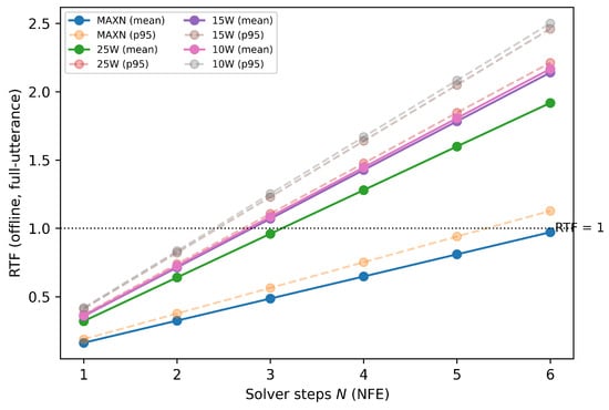
Table 10 and Figure 2 give the per-file RTF(N) sweeps at each power mode with the RTF = 1 line drawn. The quantity of interest is $N_{\max }\left(\mathrm{mode}\right)$, the largest solver-step count whose RTF stays below 1. The conventions are fixed in advance. (i) We use the per-file RTF mean. (ii) We report the full curve, not only the integer. (iii) $N_{\max }$ is corpus-dependent, bound to the VoiceBank-DEMAND duration distribution with mean 2.5146 s, where shorter utterances yield higher RTF and smaller $N_{\max }$; the p95 values are quantile estimates from the n = 100 calibrated sweeps, confirmed at the verdict steps on the full corpus.

Table 10. Solver-step budget. Per-file RTF(N) clean sweeps and $N_{\max }$ at each power mode. The upper block gives the RTF mean and the lower block the p95 (same sweeps). Full-824 confirmations at each mode’s verdict step (0.9394/0.7389/0.8215/0.8352 for MAXN/25W/15W/10W) agree with the subset p95 within 0.1%.

Mode	N = 1	N = 2	N = 3	N = 4	N = 5	N = 6	${\mathit{N}}_{\max }$ (Mean)	${\mathit{N}}_{\max }$ (p95)
MAXN	0.1625	0.3244	0.4861	0.6477	0.8097	0.9717	6	5
25W	0.3207	0.6405	0.9603	1.2800	1.5996	1.9180	3	2
15W	0.3574	0.7140	1.0705	1.4271	1.7836	2.1404	2	2
10W	0.3623	0.7236	1.0851	1.4462	1.8063	2.1669	2	2
MAXN p95	0.1888	0.3763	0.5642	0.7521	0.9401	1.1280	—	—
25W p95	0.3693	0.7387	1.1065	1.4762	1.8463	2.2119	—	—
15W p95	0.4109	0.8210	1.2297	1.6393	2.0493	2.4599	—	—
10W p95	0.4180	0.8346	1.2525	1.6693	2.0832	2.5011	—	—

Figure 2. RTF vs. solver steps at four power modes (clean sweeps, n = 100 calibrated subsets; p95 dashed).

A mean-RTF and a tail-RTF promise are different commitments. At MAXN, the mean criterion admits N = 6 (full-corpus confirmation of mean RTF 0.97294, 2.7% margin), yet 33.7% of utterances exceed RTF = 1; the service target rests on the tail criterion ($N_{\max ,\mathrm{p}95}$ = 5). At 25 W, the two criteria separate by a full step (3 vs. 2); at 15 W/10 W, both give 2. Reporting only the mean would overstate the device, so every $N_{\max }$ is labeled with its statistic. The two criteria also differ in robustness. Under the ±3.8% cross-session drift reported above, the mean criterion at the boundary is fragile, flipping outright at MAXN (N = 6 gives 0.97294 × 1.038 = 1.010, i.e., 6 ↔ 5) and surviving only barely at 25 W (N = 3 gives 0.9603 × 1.038 = 0.997), while the p95 verdicts do not move (MAXN N = 5 at 0.9394 × 1.038 = 0.975; 25 W N = 2 at 0.7389 × 1.038 = 0.767), one more reason the deployment service target rests on the tail statistic. A corpus-level p95 below one is a service target on this corpus, not a per-utterance or future-distribution guarantee.

Four checks bound the budget verdicts. First, consider estimation uncertainty. With full-824 per-file arrays retained, a filename-clustered bootstrap gives the tightest cell, MAXN N = 5, p95 0.9413 with CI [0.9268, 0.9575], the upper bound staying below RTF = 1 with ≈4.2% headroom, while N = 6 sits at 1.1278 with CI [1.1120, 1.1489] entirely above 1. Second, consider the full pipeline. A full-824 pass timing everything from disk read to output transfer gives N = 5 p95 0.9519 with a same-session paired kernel addend of +0.0123 at p95, so the MAXN verdict is unchanged with 4.8% headroom; two further clean passes give p99 = 0.98353/0.98709 with P (RTF ≥ 1) ≤ 0.61%, and the three MAXN N = 5 p95 values in this paper (0.9401 subset curve, 0.9394 confirmation, 0.9413 remeasurement) are distinct runs agreeing within 0.2%. Third, examine first-file effects. Discarding the first retained file of every pass moves the pooled p95 by at most 0.015% (0.006% at the MAXN N = 5 re-measurement), so the tail is not a cold-start or ordering artifact. Fourth, the design-stage prediction registered before any sweep measurement (2026-08-14), predicted $N_{\max }$ (mean/p95) of (5/4) at MAXN and (3/2) at 25 W, against measured (6/5) and (3/2). The extrapolation was conservative by one step, and cross-mode feasibility must be measured, not extrapolated (Section 4.3.2).

Splitting full utterances into overlapping chunks is the usual route to bounded algorithmic latency, so we measured both its quality and its device cost, both with the single-step retrained model as the tested vehicle for the flow family (the multi-step solver under chunking was not measured). On quality, the best configuration tried uses 2 s chunks, 25% overlap and a 10 ms linear edge-ramp cross-fade over the overlap regions, with the same wrapper serving the quality and cost measurements below; it loses 0.178 PESQ and 4.0 dB SI-SDR against full-utterance inference (larger than the entire truncation-versus-retraining difference, 0.173 PESQ), and 1 s chunks lose 0.33 PESQ/6.7 dB. Files at or below the 2 s chunk length (260/824, 31.6%) are processed by the full-utterance path by construction and contribute zero delta, so the files actually chunked (T > 2 s, n = 564) pay ≈ 0.26 PESQ/ 5.9 dB; either way, on the tested single-step vehicle chunking trades substantial quality for its latency bound, and whether the multi-step solver degrades identically is untested; frame-causal architectures remain the correct route to low latency. Cost is reported as a mean paired per-file ratio in the whole-function wall-clock caliber from one session, including the chunk loop, overlap-add, cross-fade and each path’s own STFT/iSTFT, and is not comparable to Table 7’s caliber. Chunking multiplies the full-utterance RTF by 1.27 at MAXN and 1.24 at every constrained mode (ratio-of-means differs by at most 0.011); the per-file p95 stays below 0.56 at every mode. The multiplier is not constant. Overlapping chunks carry an arithmetic workload ratio of 1.0–1.31 (mean 1.15; 1.0 by construction for the 31.6% fallback files, measured 1.002 ± 0.005), on top of which a per-chunk fixed overhead adds a mean of +0.12, growing with chunks per file (duration bands (2, 3] s at 1.34, (3, 5] s at 1.48, >5 s at 1.45; that band holds 17 files; non-monotone, reported as measured); per-file ratios span 0.95–1.71, the sub-unity values being timing noise on fallback files. The chunking wrapper’s full-utterance baselines come from different sessions than Table 7, so the differences (0.1632/0.3211/0.3580/0.3784 here versus 0.16246/0.32058/0.35727/0.36216 there, i.e., +0.5%, +0.2%, +0.2%, +4.5%) bound STFT, host cost and session drift jointly. Energy was not measured for the chunked configuration.

Energy supplies the dimension the RTF curve does not show. A dedicated full-824 pass at MAXN measures $E_{\mathrm{incr}}$ at every N = 1…5 in one session and yields 2189.2/4390.5/6587.4/8785.1/10995.7 mJ/s of audio. Per-step energy is constant within +0.5% (2189–2199 mJ/s per step, a slow monotone rise), and consistent within +0.2–0.7% with the cross-mode points (N = 2 at every constrained mode; N = 5/6 in the sweep sessions, per-step 2230.4 at N = 6). Solver energy is therefore measured to scale linearly with N on this board, and keeping the solver at $N^{*}$ = 4 costs 4.01× the single-step energy (8785.1 versus 2189.2 mJ/s, ≈8.8 J per audio second at MAXN), a single-board, single-corpus observation, not a law.

4.3.4. Cross-Family Same-Board Anchor

GTCRN, a 0.048 M-parameter causal CRN built for edge deployment [1], is measured on the same board, corpus and caliber, with CUDA-event timing over forward plus iSTFT and the input STFT precomputed. GTCRN’s official 512/256 window differs from ours and is reported as such. Its quality is self-measured on the same corpus and pipeline (PESQ 2.8543), not imported. The published 2.792 differs by 0.062, consistent with metric-implementation and input-configuration differences; its published RTF 0.07 is a desktop i5-12400 figure, not comparable on-device. On the other metrics, GTCRN’s SI-SDR shows no detectable difference from M3’s (18.801 versus 18.789 dB; paired t-test, p = 0.797; Wilcoxon p = 0.598; non-significance is not equivalence; no SI-SDR margin was fixed for this cross-family comparison) and it is likewise close to FlowSE N = 5 (18.845 dB). Across the three systems, SI-SDR spans only 0.06 dB while PESQ spans 0.24, so the two metrics rank the systems differently; its ESTOI trails (0.8485 versus 0.8711, paired p = 7.7 × ${10}^{-83}$).

At MAXN, GTCRN’s sustained-caliber end-to-end RTF is 16.3× lower than our single-step model’s (same-session, 0.15996/0.00981; a system-level ratio under the measured pipelines, where the two models’ STFT conventions differ, not an architecture ratio) and 25.9× at 25 W (0.31498/0.01215), both ratios sustained on both sides; per-file pairing gives 13.7×/21.9× as a sensitivity check. GTCRN’s per-file rate at MAXN is 0.01183 versus sustained 0.00981; this 17% back-to-back reduction is a measured amortization signature, not a per-kernel overhead measurement. With 1360× fewer parameters (65,590,822 versus 48,245), small parameters did not buy proportional speed here. The GPU clock drops 917 → 407 MHz while GTCRN slows only 1.24× (our models 1.97×).

The models’ different native STFTs make the following counts a comparison of network work within each measured pipeline rather than architecture alone. For the corpus-mean 2.5146 s utterance, M3 processes a 256 × 320 complex spectrogram after padding and GTCRN its native 257 × 158 input. Analytic layer-wise counts, excluding elementwise operations and iSTFT, give 332 G MACs for M3 and 0.067 G for GTCRN. The M3 estimate agrees with torch.profiler within 0.5%; GTCRN is reported analytically because the profiler omits ConvTranspose2d. The resulting operation gap is approximately $5\times {10}^3$, compared with $1360\times$ in parameters, so parameter count alone does not represent device work. Dividing these network-only counts by the measured forward-plus-iSTFT latency gives conservative effective rates of ≈1.6 TFLOP/s for M3 and ≈4 GFLOP/s for GTCRN under the two-FLOPs-per-MAC convention.

GTCRN’s lower effective rate, 1.24× slowdown under the 917 → 407 MHz clock change, and 17% back-to-back amortization are consistent with launch/dispatch sensitivity. An Nsight Systems trace tested this interpretation on one 2.5136 s utterance using four interleaved blocks of 20 recorded inferences, ordered M3 → GTCRN → GTCRN → M3. For this input, M3 issued 1453 kernels per inference, with 349.6 ms in summed kernel duration and 36.2 ms in launch-API time. GTCRN issued 293 kernels per inference; 84.8% lasted under 20 $\mathsf{\mu }$s, with a 9.3 $\mathsf{\mu }$s median, 5.0 ms summed kernel duration, and 5.6 ms launch-API time. The trace supports a launch/dispatch-sensitive interpretation for this input; the kernel and API totals are not an additive causal-overhead decomposition, and the profiled latency is not used in the RTF comparisons.

Reading each fp32 weight set once at peak memory bandwidth gives idealized time lower bounds of ≈2.6 ms for M3 and ≈2 $\mathsf{\mu }$s for GTCRN. Direct T234 DRAM-counter collection did not yield usable payloads on the tested JetPack R36.4.7/Nsight Systems 2024.5.4 configuration; achieved bandwidth and activation traffic therefore remain unavailable, and no bandwidth-bottleneck attribution is made. For DeepFilterNet2, the GEMM-only count is 0.367 G MACs/s, close to the published 0.356 [3], while the full layer-wise count including grouped GRUs is 0.96 G MACs/s; both are reported because the counting conventions may differ.

The 100 ms telemetry does not reliably resolve the short GTCRN and DFN2 executions. Table 11 therefore omits per-utterance energy for both models. Instead, all configurations are compared under a ≥60 s back-to-back sustained stream, with $E=(P_{\mathrm{loop}}-P_{\mathrm{idle}})·\mathrm{RTF}$ and RTF defined as the window’s ratio of sums. In the initial measurement campaign, GTCRN’s sustained energy was approximately 1% of the single-step model’s in both modes.

Table 11. Cross-family anchors (references, not a contest). All values in the sustained caliber (≥60 s back-to-back stream, see text; energy in millijoules per second of audio); each cell is a single sustained run. Naive within-run telemetry standard errors would understate run-level uncertainty (the 100 ms samples are autocorrelated) and are not reported; Section 4.3.1 gives the measured cross-session spread instead.

Configuration	Mode	RTF (Sustained)	Energy (mJ/s)
GTCRN	MAXN	0.00981	24.9
GTCRN	25W	0.01215	20.3
DFN2	MAXN	0.01626	173.3
DFN2	25W	0.03118	179.8
M3 (ours)	MAXN	0.15996	2214.5
FlowSE N = 1	MAXN	0.15972	2230.6
M3 (ours)	25W	0.31498	2104.1
FlowSE N = 1	25W	0.31471	2111.0

Note: The GTCRN values are from the initial measurement campaign. Later verification runs shifted its incremental-energy estimate by −12% to −18%, reflecting the sensitivity of this small power increment to board-state drift; the DFN2/GTCRN energy ratios in the text therefore use interleaved same-session adjacent blocks rather than ratios of these table cells.

DeepFilterNet2 has 2.306 M parameters and adds a native 48 kHz full-band reference. Under the declared 16 kHz → 48 kHz → enhance → 16 kHz chain, it yields PESQ 2.7449, SI-SDR 17.60 dB and ESTOI 0.841 on the same 824 utterances. The 16 kHz source limits effective bandwidth to 8 kHz, so the 0.335 PESQ gap from the published same-corpus full-band result should not be interpreted as a like-for-like model comparison.

Under the same declared per-file timing and sustained-energy calibers as GTCRN, DFN2 gives per-file RTF 0.01753 (p95 0.02633) at MAXN and 0.03226 (p95 0.04005) at 25 W, with sustained energy of 173.3 and 179.8 mJ/s. Feature extraction is outside the timed window for all models. For DFN2, the excluded preprocessing, including resampling, adds wall time approximately 0.5× its timed segment, compared with at most 10% for the flow models; the reported RTFs therefore describe the declared timed segment rather than the whole pipeline. Using the reported sustained values, DFN2’s MAXN energy is 7.8% of M3’s. In three adjacent 60 s GTCRN→DFN2 pairs sharing a common idle measurement, the median DFN2/GTCRN energy ratios were 6.76 [6.75, 7.14] at MAXN and 9.01 [9.01, 9.18] at 25 W. Because the order was fixed, these ratios are descriptive.

4.3.5. Thermal Behavior Under Sustained Load

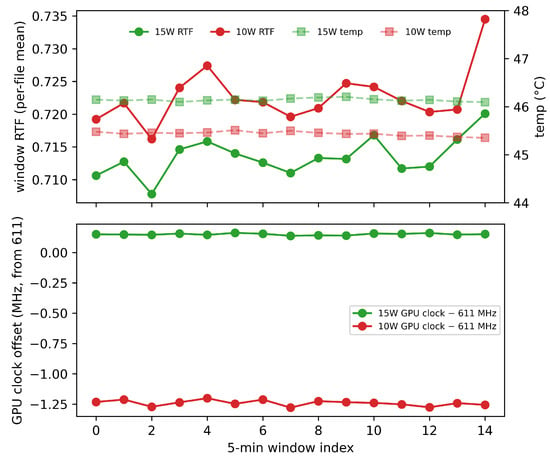
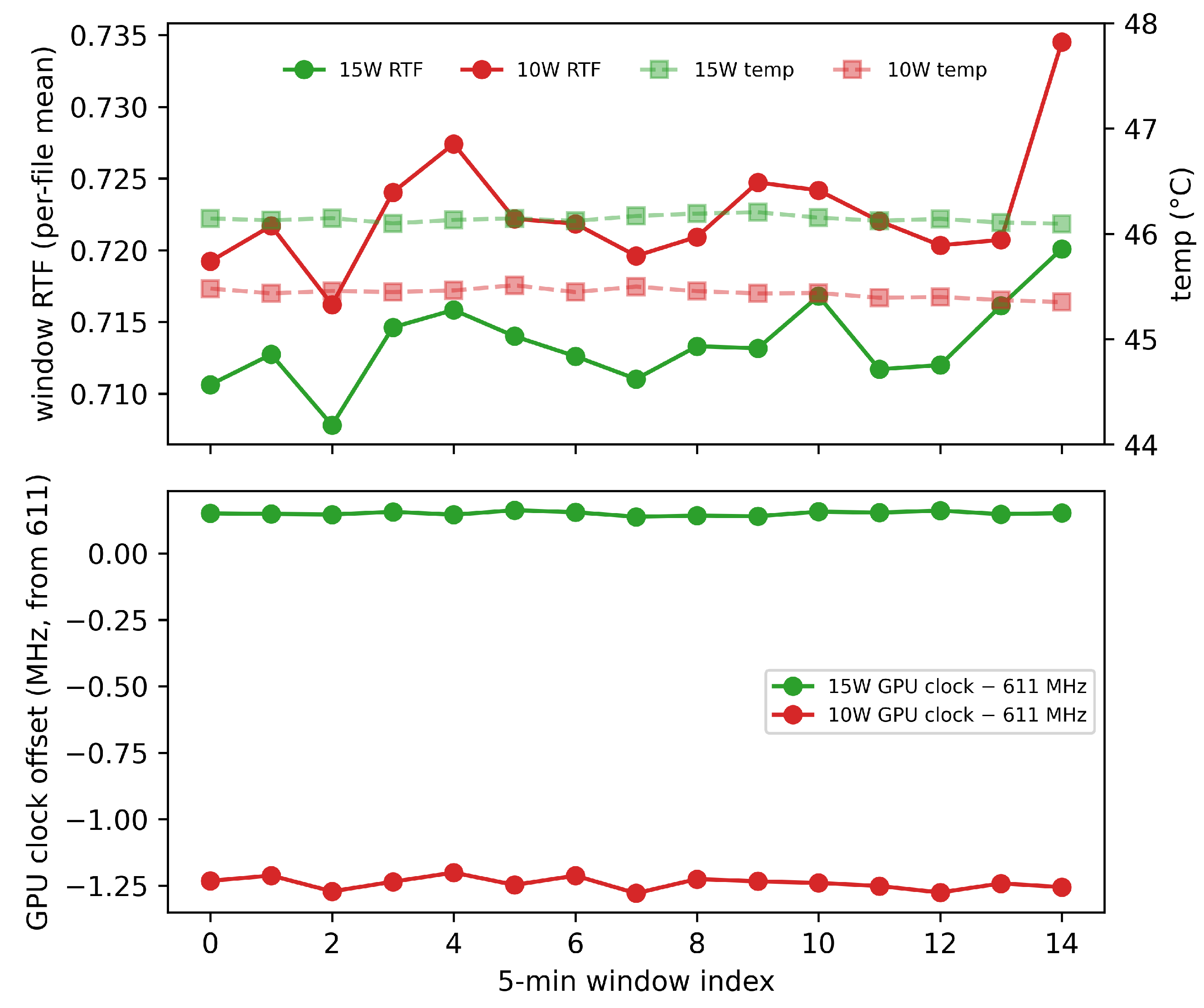
Does a configuration that passes RTF < 1 cold still pass hot? Under locked clocks and custom-fan cooling, yes. Per mode, the drift from the first to the last valid 5-min window of the sustained run, each mode at its verdict-step configuration with N = 5 at MAXN and N = 2 at the constrained modes, is +1.94% at MAXN (window temperatures averaging 59.6 °C), +0.90% at 25 W (47.3 °C, four valid windows; a fifth was excluded as incomplete), +1.33% at 15 W (46.1 °C) and +2.13% at 10 W (45.4 °C); no clock throttling was observed, and the small first-to-last RTF drift itself remains. Figure 3 shows the 15 W and 10 W traces of per-5-minute-window RTF, temperature and clock; the MAXN and 25 W windows come from the same sweep-family records. A second consistent full-824 pass hours later reproduces the mean within 0.15%.

Figure 3. Load-window (5 min) RTF/temperature/GPU clock under locked clocks, with no clock throttling observed; a small first-to-last RTF drift (+0.9% to +2.1% across modes) remains (observation, not proof).

5. Is It Worth It?

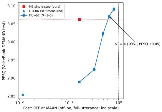
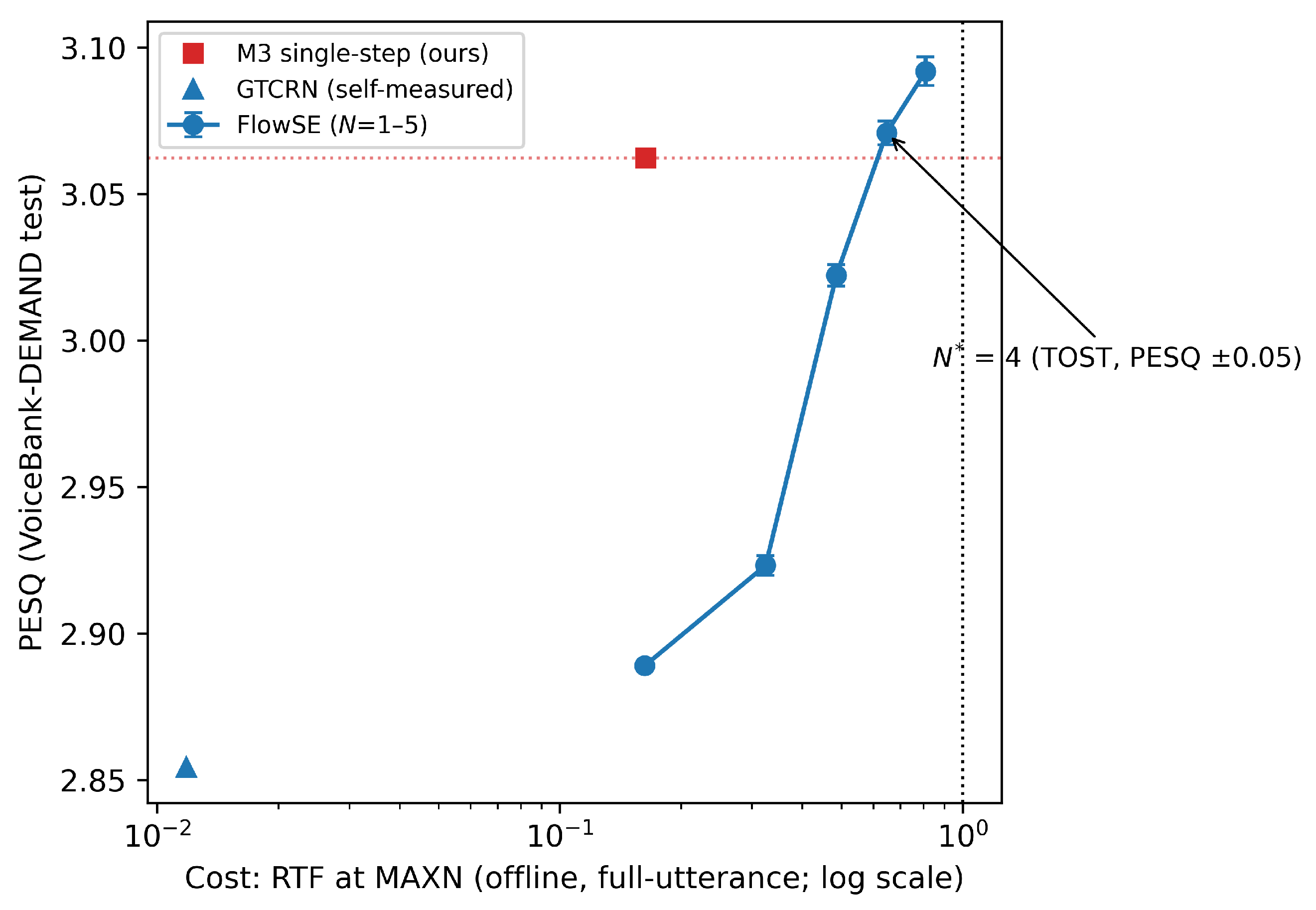
This section combines the quality-side break-even $N^{*}$ with the board-specific cost ceiling $N_{\max ,\mathrm{p}95}$ to determine which measured recipes are feasible at each power mode. Figure 4 summarizes the same-board quality–cost trade-off, and the decision rule below maps an application-specific quality floor to the measured recipes.

Figure 4. Quality (PESQ, 3 seeds ± std) vs. same-board cost (RTF at MAXN, per-file caliber). The GTCRN point uses self-measured PESQ 2.8543 (published 2.792 in text) and measured RTF. M3 and GTCRN are deterministic (no seed variation to show).

For a given power mode, with the quality criterion fixed (here, PESQ; $N^{*}$ must be re-derived per criterion) and a required quality floor $Q_{\min }$, the rule over the recipes compared in this paper reads as follows. (0) If $Q_{\min }$ ≤ 2.8543 on the chosen criterion and the compact discriminative reference meets it there (it does on PESQ; its ESTOI is lower, Section 4.3.4), take the reference, which runs at ~1% of the energy. (1) If $N_{\max ,\mathrm{p}95}$ ≥ $N^{*}$, keeping the solver is feasible and quality is comparable-or-better. (2) If $N_{\max ,\mathrm{p}95}$ < $N^{*}$ and $Q_{\min }$ ≤ 3.0622, the single-step retrained model is the strongest option at single-step cost among the measured recipes and the only one that reaches floors above the truncated N = 2 level (PESQ 2.9232) at the measured constrained modes. (3) If 3.0622 < $Q_{\min }$ ≤ 3.0709, the truncated N = 4 configuration also reaches the floor, feasible where $N_{\max ,\mathrm{p}95}$ ≥ 4. If $Q_{\min }$ > 3.0709, only the untruncated five-step FlowSE (3.0919) reaches it among the measured configurations, feasible only where $N_{\max ,\mathrm{p}95}$ ≥ 5 (here, MAXN). For $Q_{\min }$ > 3.0919 nothing measured in this study reaches the floor.

The measurement answers it, mode by mode, on this two-speaker corpus. MAXN has $N_{\max ,\mathrm{p}95}$ = 5 ≥ 4 (the solver fits); 25 W/15 W/10 W all have $N_{\max ,\mathrm{p}95}$ = 2 < 4 (it does not), and if M3-class quality is required, solver-free retraining is the only recipe compared here that reaches it at those budgets (the cost-feasible truncated N = 2 still trails M3 by 0.14 PESQ). The verdict is specific to the perceptual criterion. On SI-SDR, the same rule reads the opposite way, since the truncated solver is already better than the retrained model from one step onward (+0.7544 dB at N = 1, 90% CI [+0.711, +0.798] entirely above the ±0.5 dB band; Table 3), so under a waveform criterion the solver stays at every mode and no mode triggers retraining; ESTOI is indifferent, the two models being operationally equivalent at every N. At $N=1$, the P.808-trained predictor also favors FlowSE; no equivalence margin was defined for this metric. Both deployment boundaries are configuration-dependent. $N^{*}$ depends on the model, solver and integration grid because a different integrator may change quality per evaluation. $N_{\max }$ depends on measured runtime and must be re-derived whenever an optimization changes the timed path. We evaluated two practical Jetson runtime options without exporting the complex-domain backbone. In eager PyTorch 2.11.0, tensors remain in fp32/complex64, while cuDNN convolutions use TF32 arithmetic. Relative to this path, disabling TF32 increased paired per-file forward+iSTFT latency by 1.911× at MAXN and 2.044× at 25 W. The maximum absolute waveform difference between the two settings was 1.4 × ${10}^{-4}$; the PESQ effect was not measured. Fixed-shape, forward-only CUDA Graph reduced forward latency by 1.8–2.4%. This gain applies only to the capturable forward segment because full forward+iSTFT capture did not succeed, so it is not used to recompute RTF or $N_{\max }$. The comparison is limited to these PyTorch 2.11.0 runtime paths. Full-model fp16 casting and autocast did not yield valid outputs in this implementation, and TensorRT was not evaluated. Three constrained modes reach the same verdict consistently, a robustness pattern from the same board, corpus and measurement code rather than independent replications, and the 25 W verdict holds for both statistics (mean 3, p95 2, both < 4), for every equivalence margin tested ($\delta$∈ [0.03, 0.08] gives $N^{*}$∈ {3, 4}, both > 2), and at both hot and cold states. Every retrained anchor measured, five replicates in total, gives $N^{*}$ = 3, against 4 for the original M3. Where the solver does not fit, M3 buys +0.1733 PESQ over the truncated N = 1 configuration at identical device cost, in the tested realizations (seven-metric reading in Section 3). One boundary is that $N^{*}$ and this gap are measured on the matched VoiceBank–DEMAND distribution. The DNS check below extends the quality comparison to a jointly shifted speech, noise and mixing distribution, so it serves as a distribution-level check rather than an isolated test of noise shift.

Together, the solver-budget results, Table 12 and Figure 4 show a measured, criterion-dependent trade-off. At MAXN, $N^{*}=4$ is feasible with 25% p95 RTF headroom. At 25 W, 15 W and 10 W, $N_{\max ,\mathrm{p}95}=2$, so the feasible N = 2 solver remains 0.14 PESQ below M3. The compact GTCRN anchor occupies the low-cost, lower-PESQ end of the trade-off. In Table 11’s matched sustained comparison at MAXN, its RTF is $1/16.3$ of M3’s and its energy is about 1% of M3’s, with PESQ 0.208 lower. A paired SI-SDR test did not detect a difference ($p=0.797$). Thus, among the measured recipes, the choice depends on the application’s quality floor and the board-specific $N_{\max }$.

Table 12. Same-board quality–cost points. Quality is PESQ on the full 824-utterance set, computed with the same evaluator after each model’s declared preprocessing chain (3 seeds for the stochastic model). Cost is per-file RTF from the sweep family, every row its own measurement; FlowSE N = 1 and M3 differ by at most 0.04%.

Model/Configuration	PESQ	RTF @ MAXN	RTF @ 25 W	Energy @ MAXN (mJ/s)
GTCRN	2.8543	0.01183	0.01465	24.9
DFN2	2.7449	0.01753	0.03226	173.3
FlowSE N = 1	2.8890	0.1625	0.3207	2189.2
FlowSE N = 2	2.9232	0.3244	0.6405	4390.5
FlowSE N = 4	3.0709	0.6477	1.2800	8785.1
FlowSE N = 5	3.0919	0.8097	1.5996	10995.7
M3 (ours)	3.0622	0.1625	0.3206	2218.3

Note: Energy is reported under two declared calibers. The FlowSE and M3 cells come from dedicated full-824 utterance-stream passes, whereas the GTCRN and DFN2 cells use sustained streams (Section 4.3.4) because 100 ms telemetry does not reliably resolve their short per-utterance executions. Energy values should therefore be compared within, rather than across, these calibers. The DFN2 PESQ cell follows the declared 16 kHz → 48 kHz → enhance → 16 kHz chain (Section 4.3.4).

The matched-caliber procedure specifies a measurement sequence and separates it from configuration-specific outputs. It labels per-file, sustained-stream, and whole-function timing, pairs drift-sensitive ratios within sessions, reports drift and deployment uncertainty, and combines quality-side $N^{*}$ with board-specific $N_{\max }$ under offline RTF < 1. The reported $N_{\max }$ values, energies, and cross-family ratios are board- and runtime-specific. The PESQ value $N^{*}=4$ is conditional on the model, solver, criterion and margin, evaluation distribution, and numerical arithmetic. The two VoiceBank test speakers yield $N^{*}$ values of 3 and 4, and the VCTK and DNS checks below reinforce that $N^{*}$ depends on the evaluation distribution. With numerical outputs preserved, moving to new hardware requires remeasuring $N_{\max }$ but not $N^{*}$. Any change to a quality-side factor requires re-estimating $N^{*}$ against a retrained reference. The procedure is specified for reapplication but has not yet been empirically validated beyond this configuration.

In the DNS-2020 distribution check, the frozen models were evaluated without tuning on 150 paired no-reverb clips from the open synthetic set [47]. Its clean-speech source corpus has 20 speakers, but unavailable clip-to-speaker mappings make this a corpus-level rather than speaker-level check. No tested $N\le 5$ entered the ±0.05 PESQ band. At $N=5$, FlowSE remained 0.116 below M3, with 90% CI [−0.150, −0.083], compared with $N^{*}=4$ on VoiceBank–DEMAND. This contrast is consistent with $N^{*}$ being evaluation-distribution-conditional. At $N=1$, SI-SDR and ESTOI lie within their equivalence bands, so criterion dependence persists on this set. On a separate 150-pair with-reverb stress test, both models score below the noisy input on all three metrics, marking a shared out-of-distribution failure rather than a speaker-diversity result.

Separately, the VCTK held-out-speaker check used 200 mixtures from 20 speakers excluded from the VoiceBank–DEMAND training and test speakers [48]. Each speaker contributed 10 utterances mixed with three DEMAND scenes at 2.5, 7.5, 12.5, and 17.5 dB. The frozen models were evaluated without retraining or tuning. With speaker as the inference unit ($n=20$), M3’s mean PESQ exceeds FlowSE’s at every tested $N=1$–5. At $N=1$–4, the 90% CIs for the FlowSE–M3 difference lie entirely below zero. At $N=5$, M3’s mean advantage is 0.025 PESQ, while the 90% CI for FlowSE–M3 is [−0.069, +0.019]. SI-SDR favors FlowSE throughout and enters its equivalence band at $N=5$, while ESTOI is equivalent throughout. Thus, within this constructed 20-speaker check, M3 remains PESQ-competitive and the ranking remains criterion-dependent.

Choosing the criterion is the practitioner’s first decision and should follow the application endpoint rather than model ranking (Section 3). At one forward pass on this corpus, M3 leads on PESQ, FlowSE leads on SI-SDR, and ESTOI is operationally equivalent. The SI-SDR and ESTOI relations persist across all tested step counts. Practitioners should fix the corresponding quality floor and equivalence margin before measurement. Where no standardized margin exists, the verdict should be reported over a sensitivity interval. Here, $\delta \in [0.03,0.08]$ gives $N^{*}\in \{3,4\}$ and leaves every mode-level deployment verdict unchanged. The procedure requires one retrained reference rather than repeated training for each board. For a fixed model, solver, criterion, margin, evaluation distribution and numerical arithmetic, derive $N^{*}$ once against that reference. Section 4.2 shows that a warm-started single-stage run supplies it. Then derive $N_{\max }$ on each target board and mode without retraining.

The uncertainty bounds relevant to the main verdicts are as follows:

• Energy repeatability. Cross-session single-step energy varies by 0.17–1.33% across 2189.2–2218.3 mJ/s measurements (Section 4.3.1); these are internal repeatability checks, not external calibration.
• Post-hoc energy band. With idle-drift uncertainty propagated, the constant-energy verdict is indeterminate at 25 W, depends on the registered versus final band at 15 W, and is robust at 10 W under both bands (Section 4.3.1).
• Deployment verdict. The largest observed cross-session RTF spread is 3.8%, below the tightest p95 verdict-flip margin of 6.4% at MAXN; all p95 $N_{\max }$ decisions therefore remain unchanged.

Thus, the p95 deployment decisions are robust to the observed drift, whereas the constant-energy conclusion is robust only at 10 W.

6. Conclusions

This paper asked what a generative flow-matching speech enhancer actually costs on a power-constrained embedded GPU, and answered with a conditional decision rule built from two measured quantities, the quality-side break-even $N^{*}$ = 4 solver steps (PESQ caliber) and the cost-side ceiling $N_{\max }$. On the Jetson Orin NX, under the stated PESQ criterion and ±0.05 margin, the solver fits at the unconstrained mode ($N_{\max ,\mathrm{p}95}$ = 5 ≥ 4). At every constrained budget (25/15/10 W), it does not ($N_{\max ,\mathrm{p}95}$ = 2 < 4), and the single-step retrained model is the only recipe compared here that reaches retrained quality. At identical device cost, it gains +0.17 PESQ over truncation while losing 0.75 dB of waveform fidelity. Three findings delimit this decision. Power modes are not a performance axis, so cost must be measured per mode. Incremental energy is not constant across budgets (2218 vs. 2022 mJ/s, outside ±5% under both the final and the as-registered analysis bands). At MAXN, the 0.048 M-parameter discriminative reference runs at 1/16.3 of M3’s sustained-caliber end-to-end RTF and about 1% of its energy, with PESQ 0.208 lower. It therefore brackets the measured trade-off from below. The matched-caliber procedure specifies what a target deployment must repeat. $N_{\max }$ is re-measured on the target board, whereas $N^{*}$ is re-estimated against one retrained reference whenever the model, solver, criterion or margin, evaluation distribution, or numerical arithmetic changes. Section 4.2 shows that warm-started single-stage training supplies this reference. The present empirical validation is limited to the tested configuration. The same measurement question may arise for diffusion-based electrocardiogram (ECG) [49] and electroencephalogram (EEG) [50] denoising, while compact discriminative biosignal models already operate at microcontroller power [51]. Applying the $N^{*}$–$N_{\max }$ framing to these signals is a methodological analogy. Their µW-to-mW platforms require task- and device-specific measurements.

All device measurements and the primary quality–cost verdict come from one Orin NX and the 824-utterance, two-speaker VoiceBank–DEMAND test set. The quality-side scope is broadened by a held-out-speaker VCTK check over 20 speaker clusters and a DNS-2020 corpus-level distribution check. The primary comparisons use one run per training configuration, while the training-realization check spans three warm-recipe seeds and two replicas of the reference chain’s final three stages. The reported RTF includes the inverse STFT and remains corpus-duration-dependent; 100 ms telemetry does not reliably resolve per-utterance energy for sub-30 ms workloads. Under continuous load, the default dynamic voltage and frequency scaling (DVFS) governor differs from locked clocks by −0.20% in mean and −0.12% at p95 across eight interleaved arms in two sessions, with the governor at maximum clock throughout. The uniform RTF inflation required to flip each p95 verdict ranges from +6.4% at MAXN to +35% at 25 W. Even the tightest margin is 1.7× the largest measured cross-session drift of 3.8%, while the absolute governor difference is 0.20%. By contrast, the mean-based MAXN verdict at N = 6 has a 2.7% margin and would flip under a uniform 3.8% inflation. This supports using p95 rather than the mean as the deployment service target. The tested scope is offline full-utterance inference under continuous load; bursty or low-duty-cycle operation and streaming causal architectures remain future work.

References

- Rong, X.; Sun, T.; Zhang, X.; Hu, Y.; Zhu, C.; Lu, J. GTCRN: A Speech Enhancement Model Requiring Ultralow Computational Resources. In Proceedings of the IEEE International Conference on Acoustics, Speech and Signal Processing (ICASSP), Seoul, Republic of Korea, 14–19 April 2024; IEEE: New York, NY, USA, 2024; pp. 971–975. [Google Scholar] [CrossRef] [Scilit]
- Wahab, F.E.; Ye, Z.; Saleem, N.; Ullah, R. Compact Deep Neural Networks for Real-Time Speech Enhancement on Resource-Limited Devices. Speech Commun. 2024, 156, 103008. [Google Scholar] [CrossRef] [Scilit]
- Schröter, H.; Maier, A.; Escalante-B., A.N.; Rosenkranz, T. DeepFilterNet2: Towards Real-Time Speech Enhancement on Embedded Devices for Full-Band Audio. In Proceedings of the International Workshop on Acoustic Signal Enhancement (IWAENC), Bamberg, Germany, 5–8 September 2022. [Google Scholar] [CrossRef] [Scilit]
- Lee, S.; Cheong, S.; Han, S.; Shin, J.W. FlowSE: Flow Matching-Based Speech Enhancement. In Proceedings of the IEEE International Conference on Acoustics, Speech and Signal Processing (ICASSP), Hyderabad, India, 6–11 April 2025; IEEE: New York, NY, USA, 2025; pp. 1–5. [Google Scholar] [CrossRef] [Scilit]
- Wang, Z.; Liu, Z.; Zhu, X.; Zhu, Y.; Liu, M.; Chen, J.; Xiao, L.; Weng, C.; Xie, L. FlowSE: Efficient and High-Quality Speech Enhancement via Flow Matching. In Proceedings of 26th Interspeech Conference, Rotterdam, The Netherlands, 17–21 August 2025; ISCA—International Speech Communication Association: Grenoble, France, 2025; pp. 4858–4862. [Google Scholar] [CrossRef] [Scilit]
- Lipman, Y.; Chen, R.T.Q.; Ben-Hamu, H.; Nickel, M.; Le, M. Flow Matching for Generative Modeling. In Proceedings of the Eleventh International Conference on Learning Representations (ICLR), Kigali, Rwanda, 1–5 May 2023; Available online: https://iclr.cc/virtual/2023/poster/11309 (accessed on 1 October 2026).
- Song, Y.; Sohl-Dickstein, J.; Kingma, D.P.; Kumar, A.; Ermon, S.; Poole, B. Score-Based Generative Modeling through Stochastic Differential Equations. In Proceedings of the Ninth International Conference on Learning Representations (ICLR), Virtual Event, Austria, 3–7 May 2021; Available online: https://iclr.cc/virtual/2021/poster/3177 (accessed on 1 October 2026).
- Welker, S.; Lay, B.; Hillemann, M.; Peer, T.; Gerkmann, T. Real-Time Streamable Generative Speech Restoration with Flow Matching. IEEE Trans. Audio Speech Lang. Process. 2026, 34, 3087–3101. [Google Scholar] [CrossRef] [Scilit]
- Lemercier, J.-M.; Richter, J.; Welker, S.; Gerkmann, T. StoRM: A Diffusion-Based Stochastic Regeneration Model for Speech Enhancement and Dereverberation. IEEE/ACM Trans. Audio Speech Lang. Process. 2023, 31, 2724–2737. [Google Scholar] [CrossRef] [Scilit]
- Lay, B.; Lemercier, J.-M.; Richter, J.; Gerkmann, T. Single and Few-Step Diffusion for Generative Speech Enhancement. In Proceedings of the IEEE International Conference on Acoustics, Speech and Signal Processing (ICASSP), Seoul, Republic of Korea, 14–19 April 2024; IEEE: New York, NY, USA, 2024; pp. 626–630. [Google Scholar] [CrossRef] [Scilit]
- Trachu, T.; Piansaddhayanon, C.; Chuangsuwanich, E. Thunder: Unified Regression-Diffusion Speech Enhancement with a Single Reverse Step using Brownian Bridge. In Proceedings of Interspeech, Kos Island, Greece, 1–5 September 2024; ISCA—International Speech Communication Association: Grenoble, France, 2024; pp. 1180–1184. [Google Scholar] [CrossRef] [Scilit]
- Zhu, Y.; Kang, B.; Wang, Z.; Li, X.; Zhang, Z.; Li, W.; Xiao, L.; Xue, W.; Xie, L. MeanFlowSE: One-Step Generative Speech Enhancement via MeanFlow. arXiv 2025, arXiv:2509.23299. [Google Scholar]
- Li, D.; Lu, S.; Pan, H.; Zhan, Z.; Hong, Q.; Li, L. MeanFlowSE: One-Step Generative Speech Enhancement via Conditional Mean Flow. In Proceedings of the IEEE International Conference on Acoustics, Speech and Signal Processing (ICASSP), Barcelona, Spain, 4–8 May 2026; IEEE: New York, NY, USA, 2026; pp. 16172–16176. [Google Scholar] [CrossRef] [Scilit]
- Lay, B.; Makarov, R.; Gerkmann, T. Diffusion Buffer: Online Diffusion-Based Speech Enhancement with Sub-Second Latency. In Proceedings of Interspeech, Rotterdam, The Netherlands, 17–21 August 2025; ISCA—International Speech Communication Association: Grenoble, France, 2025; pp. 793–797. [Google Scholar] [CrossRef] [Scilit]
- Lay, B.; Makarov, R.; Welker, S.; Hillemann, M.; Gerkmann, T. Diffusion Buffer for Online Generative Speech Enhancement. IEEE Trans. Audio Speech Lang. Process. 2026, 34, 3476–3490. [Google Scholar] [CrossRef] [Scilit]
- Hsieh, T.-A.; Braun, S. Towards Real-Time Generative Speech Restoration with Flow-Matching. In Proceedings of the IEEE International Conference on Acoustics, Speech and Signal Processing (ICASSP), Barcelona, Spain, 4–8 May 2026; IEEE: New York, NY, USA, 2026; pp. 15847–15851. [Google Scholar] [CrossRef] [Scilit]
- Song, Y.; Dhariwal, P.; Chen, M.; Sutskever, I. Consistency Models. In Proceedings of the 40th International Conference on Machine Learning (ICML), Honolulu, HI, USA, 23–29 July 2023; Volume 202, pp. 32211–32252. Available online: https://proceedings.mlr.press/v202/song23a.html (accessed on 1 October 2026).
- Xu, L.; Yan, L.F.; Kleijn, W.B. Robust One-Step Speech Enhancement via Consistency Distillation. In Proceedings of the IEEE Workshop on Applications of Signal Processing to Audio and Acoustics (WASPAA), Tahoe City, CA, USA, 12–15 October 2025; IEEE: New York, NY, USA, 2025; pp. 1–5. [Google Scholar] [CrossRef] [Scilit]
- Lee, L.; Ji, Y.; Lee, M.; Choi, M.-S. DEMUCS-Mobile: On-Device Lightweight Speech Enhancement. In Proceedings of Interspeech, Brno, Czech Republic, 30 August–3 September 2021; ISCA—International Speech Communication Association: Grenoble, France, 2021; pp. 2711–2715. [Google Scholar] [CrossRef] [Scilit]
- Rusci, M.; Fariselli, M.; Croome, M.; Paci, F.; Flamand, E. Accelerating RNN-Based Speech Enhancement on a Multi-Core MCU with Mixed FP16-INT8 Post-Training Quantization. In Proceedings of the ITEM Workshop, ECML-PKDD, Grenoble, France, 19 September 2022. [Google Scholar] [CrossRef] [Scilit]
- Shankar, N.; Bhat, G.S.; Panahi, I.M.S. Real-Time Single-Channel Deep Neural Network-Based Speech Enhancement on Edge Devices. In Proceedings of Interspeech, Shanghai, China, 25–29 October 2020; ISCA—International Speech Communication Association: Grenoble, France, 2020; pp. 3281–3285. [Google Scholar] [CrossRef] [Scilit] [PubMed]
- Rong, X.; Yang, L.; Wang, D.; Hu, Y.; Zhu, C.; Chen, K.; Lu, J. UL-UNAS: Ultra-Lightweight U-Nets for Real-Time Speech Enhancement via Network Architecture Search. IEEE Trans. Audio Speech Lang. Process. 2026, 34, 1085–1096. [Google Scholar] [CrossRef] [Scilit]
- Xi, J.; Xu, Z.; Zhang, W.; Zhao, L.; Xie, Y. Speech Enhancement Algorithm Based on Microphone Array and Lightweight CRN for Hearing Aid. Electronics 2024, 13, 4394. [Google Scholar] [CrossRef] [Scilit]
- Kim, S.M. Frequency-Aware Multi-Rate Resampling with Multi-Band Deep Supervision for Modular Speech Denoising. Electronics 2025, 14, 4523. [Google Scholar] [CrossRef] [Scilit]
- NVIDIA Corporation. Riva Speech AI SDK. Available online: https://developer.nvidia.com/riva (accessed on 18 August 2026).
- NVIDIA-AI-IOT. Jetson Benchmarks. Available online: https://github.com/NVIDIA-AI-IOT/jetson_benchmarks (accessed on 18 August 2026).
- Lu, Y.-X.; Ai, Y.; Ling, Z.-H. MP-SENet: A Speech Enhancement Model with Parallel Denoising of Magnitude and Phase Spectra. In Proceedings of Interspeech, Dublin, Ireland, 20–24 August 2023; ISCA—International Speech Communication Association: Grenoble, France, 2023; pp. 3834–3838. [Google Scholar] [CrossRef] [Scilit]
- Chao, R.; Cheng, W.-H.; La Quatra, M.; Siniscalchi, S.M.; Yang, C.-H.H.; Fu, S.-W.; Tsao, Y. An Investigation of Incorporating Mamba for Speech Enhancement. In Proceedings of the IEEE Spoken Language Technology Workshop (SLT), Macao, China, 2–5 December 2024; IEEE: New York, NY, USA; Volume 2024, pp. 302–308. [Google Scholar] [CrossRef] [Scilit]
- Yan, M.; Wang, H.; Venkataraman, S. PolyThrottle: Energy-Efficient Neural Network Inference on Edge Devices. arXiv 2023, arXiv:2310.19991. [Google Scholar]
- Wang, R.; Lin, F.X. Turbocharge Speech Understanding with Pilot Inference. In Proceedings of the ACM International Conference on Mobile Computing and Networking (MobiCom), Washington, DC, USA, 18–22 November 2024. [Google Scholar] [CrossRef] [Scilit]
- He, K.; Zhang, X.; Ren, S.; Sun, J. Deep Residual Learning for Image Recognition. In Proceedings of the IEEE Conference on Computer Vision and Pattern Recognition (CVPR), Las Vegas, NV, USA, 26 June–1 July 2016; IEEE: New York, NY, USA, 2016; pp. 770–778. [Google Scholar] [CrossRef] [Scilit]
- Lemercier, J.-M.; Richter, J.; Welker, S.; Gerkmann, T. Analysing Diffusion-Based Generative Approaches Versus Discriminative Approaches for Speech Restoration. In Proceedings of the IEEE International Conference on Acoustics, Speech and Signal Processing (ICASSP), Rhodes Island, Greece, 4–10 June 2023. [Google Scholar] [CrossRef] [Scilit]
- Valentini-Botinhao, C.; Wang, X.; Takaki, S.; Yamagishi, J. Investigating RNN-Based Speech Enhancement Methods for Noise-Robust Text-to-Speech. In Proceedings of the ISCA Speech Synthesis Workshop (SSW), Sunnyvale, CA, USA, 13–15 September 2016; ISCA—International Speech Communication Association: Grenoble, France, 2016; pp. 146–152. [Google Scholar] [CrossRef] [Scilit]
- Kong, J.; Kim, J.; Bae, J. HiFi-GAN: Generative Adversarial Networks for Efficient and High Fidelity Speech Synthesis. In Proceedings of Advances in Neural Information Processing Systems (NeurIPS), Vancouver, BC, Canada, 6–12 December 2020; Curran Associates Inc.: Red Hook, NY, USA, 2020; Volume 33, pp. 17022–17033. Available online: https://proceedings.neurips.cc/paper/2020/hash/c5d736809766d46260d816d8dbc9eb44-Abstract.html (accessed on 1 October 2026).
- Rix, A.W.; Beerends, J.G.; Hollier, M.P.; Hekstra, A.P. Perceptual Evaluation of Speech Quality (PESQ)—A New Method for Speech Quality Assessment of Telephone Networks and Codecs. In Proceedings of the IEEE International Conference on Acoustics, Speech and Signal Processing (ICASSP), Salt Lake City, UT, USA, 7–11 May 2001; IEEE: New York, NY, USA, 2001; pp. 749–752. [Google Scholar] [CrossRef] [Scilit]
- ITU-T. Recommendation P.862.2: Wideband Extension to Recommendation P.862 for the Assessment of Wideband Telephone Networks and Speech Codecs; International Telecommunication Union: Geneva, Switzerland, 2007; Available online: https://www.itu.int/rec/R-REC-P.862.2-200711-I/en (accessed on 24 August 2026).
- Le Roux, J.; Wisdom, S.; Erdogan, H.; Hershey, J.R. SDR—Half-Baked or Well Done? In Proceedings of the IEEE International Conference on Acoustics, Speech and Signal Processing (ICASSP), Brighton, UK, 12–17 May 2019; IEEE: New York, NY, USA, 2019; pp. 626–630. [Google Scholar] [CrossRef] [Scilit]
- Jensen, J.; Taal, C.H. An Algorithm for Predicting the Intelligibility of Speech Masked by Modulated Noise Maskers. IEEE/ACM Trans. Audio Speech Lang. Process. 2016, 24, 2009–2022. [Google Scholar] [CrossRef] [Scilit]
- Reddy, C.K.A.; Gopal, V.; Cutler, R. DNSMOS P.835: A Non-Intrusive Perceptual Objective Speech Quality Metric to Evaluate Noise Suppressors. In Proceedings of the IEEE International Conference on Acoustics, Speech and Signal Processing (ICASSP), Singapore, 22–27 May 2022; IEEE: New York, NY, USA, 2022; pp. 886–890. [Google Scholar] [CrossRef] [Scilit]
- ITU-T. Recommendation P.808: Subjective Evaluation of Speech Quality with a Crowdsourcing Approach; International Telecommunication Union: Geneva, Switzerland, 2018; Available online: https://www.itu.int/rec/R-REC-P.808-201809-I/en (accessed on 24 August 2026).
- Hu, Y.; Loizou, P.C. Evaluation of Objective Quality Measures for Speech Enhancement. IEEE Trans. Audio Speech Lang. Process. 2008, 16, 229–238. [Google Scholar] [CrossRef] [Scilit]
- Rix, A.W.; Beerends, J.G.; Kim, D.-S.; Kroon, P.; Ghitza, O. Objective Assessment of Speech and Audio Quality—Technology and Applications. IEEE Trans. Audio Speech Lang. Process. 2006, 14, 1890–1901. [Google Scholar] [CrossRef] [Scilit]
- Richter, J.; Welker, S.; Lemercier, J.-M.; Lay, B.; Gerkmann, T. Speech Enhancement and Dereverberation with Diffusion-Based Generative Models. IEEE/ACM Trans. Audio Speech Lang. Process. 2023, 31, 2351–2364. [Google Scholar] [CrossRef] [Scilit]
- Chhaglani, B.; Gao, Y.; Richter, J.; Li, X.; Zadissa, S.; Pruthi, T.; Lovitt, A. ArtiFree: Detecting and Reducing Generative Artifacts in Diffusion-Based Speech Enhancement. In Proceedings of the IEEE International Conference on Acoustics, Speech and Signal Processing (ICASSP), Barcelona, Spain, 4–8 May 2026. [Google Scholar] [CrossRef] [Scilit]
- de Oliveira, D.; Welker, S.; Richter, J.; Gerkmann, T. The PESQetarian: On the Relevance of Goodhart’s Law for Speech Enhancement. In Proceedings of the Interspeech, Kos Island, Greece, 1–5 September 2024. [Google Scholar] [CrossRef] [Scilit]
- Xu, Y.; Du, J.; Dai, L.-R.; Lee, C.-H. An Experimental Study on Speech Enhancement Based on Deep Neural Networks. IEEE Signal Process. Lett. 2014, 21, 65–68. [Google Scholar] [CrossRef] [Scilit]
- Reddy, C.K.A.; Gopal, V.; Cutler, R.; Beyrami, E.; Cheng, R.; Dubey, H.; Matusevych, S.; Aichner, R.; Aazami, A.; Braun, S.; et al. The INTERSPEECH 2020 Deep Noise Suppression Challenge: Datasets, Subjective Testing Framework, and Challenge Results. In Proceedings of the Interspeech, Shanghai, China, 25–29 October 2020; ISCA—International Speech Communication Association: Grenoble, France, 2020; pp. 2492–2496. [Google Scholar] [CrossRef] [Scilit]
- Veaux, C.; Yamagishi, J.; MacDonald, K. CSTR VCTK Corpus: English Multi-Speaker Corpus for CSTR Voice Cloning Toolkit [Sound]; University of Edinburgh, Centre for Speech Technology Research (CSTR): Edinburgh, UK, 2017. [Google Scholar] [CrossRef]
- Li, H.; Ditzler, G.; Roveda, J.M.; Li, A. DeScoD-ECG: Deep Score-Based Diffusion Model for ECG Baseline Wander and Noise Removal. IEEE J. Biomed. Health Inform. 2024, 28, 5081–5091. [Google Scholar] [CrossRef] [Scilit] [PubMed]
- Huang, X.; Li, C.; Liu, A.; Qian, R.; Chen, X. EEGDfus: A Conditional Diffusion Model for Fine-Grained EEG Denoising. IEEE J. Biomed. Health Inform. 2025, 29, 2557–2569. [Google Scholar] [CrossRef] [Scilit] [PubMed]
- Cinotti, E.; Gragnaniello, M.; Parlato, S.; Centracchio, J.; Andreozzi, E.; Bifulco, P.; Riccio, M.; Esposito, D. An Edge AI Approach for Low-Power, Real-Time Atrial Fibrillation Detection on Wearable Devices Based on Heartbeat Intervals. Sensors 2025, 25, 7244. [Google Scholar] [CrossRef] [Scilit] [PubMed]
Disclaimer/Publisher’s Note: The statements, opinions and data contained in all publications are solely those of the individual author(s) and contributor(s) and not of MDPI and/or the editor(s). MDPI and/or the editor(s) disclaim responsibility for any injury to people or property resulting from any ideas, methods, instructions or products referred to in the content. |
© 2026 by the authors. Licensee MDPI, Basel, Switzerland. This article is an open access article distributed under the terms and conditions of the Creative Commons Attribution (CC BY) license.