


Abstract
Accurate remaining useful life (RUL) prediction for aero-engines is important for condition-based maintenance and safety-oriented health management. Long short-term memory (LSTM) networks are widely used for this task, but two limitations remain important in multi-sensor degradation modeling: hidden states generated over the full window are often under-utilized, and attention mechanisms may overemphasize locally fluctuating sensor readings. This paper proposes a Multi-Statistic Disentangled LSTM (MSD-LSTM) framework for aero-engine RUL prediction. The framework first applies Savitzky–Golay filtering to smooth high-frequency signal fluctuations. A hidden-state feature extraction module then combines feature-level disentangled extraction and Global Average Pooling to use the LSTM hidden-state sequence beyond the final recurrent output. In parallel, a Multi-Statistic Pooler summarizes each input window using minimum, maximum, standard deviation, and mean statistics, and its output is fused with a self-attention branch through a static-gating mechanism. On the NASA C-MAPSS benchmark, MSD-LSTM achieves RMSE values of 10.45 and 12.33 on FD001 and FD002, respectively, and ranks first in RMSE on three of the four sub-datasets and first in SCORE on two sub-datasets among the compared recent methods. Ablation and fusion analyses show that both the hidden-state extraction and statistic-guided fusion components contribute to stable RUL prediction.
1. Introduction
Aero-engines operate under complex thermo-mechanical loads, and their degradation is reflected by high-dimensional sensor streams collected across long flight-cycle histories. Remaining useful life (RUL) prediction is therefore a central task in prognostics and health management (PHM), because a reliable estimate of the remaining operating cycles supports condition-based maintenance, reduces unscheduled downtime, and helps avoid late maintenance decisions in safety-critical aviation systems [1,2,3]. Data-driven RUL prediction has become especially important because modern engine degradation is shaped by coupled subsystems and operating conditions that are difficult to describe with a single explicit physical model [4,5,6].
Deep neural networks have been widely used to learn degradation representations directly from multi-sensor time series. Among them, long short-term memory (LSTM) networks remain a common backbone for aero-engine RUL prediction because their gated memory structure can model long-range temporal dependencies [7,8]. Attention-enhanced LSTM variants, CNN–LSTM hybrids, temporal convolutional models, graph-based models, and Transformer-like architectures have further improved the representation of temporal and cross-sensor dependencies [9,10,11,12]. Earlier condition-monitoring work on helicopter units and recent stochastic engine-usage optimization for fighter-jet fleets further show that machinery diagnosis and engine health assessment are tied to maintenance planning and fleet-level operational decisions, not only to isolated fault recognition [13,14]. Recent C-MAPSS studies have combined evolutionary optimization, recurrent modeling, attention-enhanced LSTM, lightweight CNN–LSTM structures, and implicit equilibrium modeling for turbofan or aircraft-engine RUL prediction [15,16,17,18]. Related equipment RUL studies also point to the importance of flexible feature fusion and limited-data learning in deep prognostic models [19]. Statistics-aware attention and multi-scale fusion have likewise been explored for aero-engine RUL prediction [20,21]. These studies leave a practical modeling question: how to combine attention-based temporal cues with stable window-level statistics while still using the hidden-state sequence produced by the LSTM.
Two practical issues motivate the present study. First, conventional LSTM-based predictors often rely primarily on the final hidden state or on a simple aggregation of recurrent outputs. This design can under-utilize the hidden-state sequence generated over the full sliding window, even though early and intermediate hidden states may contain useful information about gradual degradation. Second, attention mechanisms are effective for emphasizing informative time steps, but their learned weights do not explicitly distinguish between stable degradation signatures and locally fluctuating sensor readings. If a locally abnormal timestamp receives a high attention weight, the resulting representation may become sensitive to short-term perturbations rather than to the underlying degradation trend.
To address these issues, this paper proposes a Multi-Statistic Disentangled LSTM (MSD-LSTM) framework for aero-engine RUL prediction. The model uses Savitzky–Golay (SG) filtering as an input-level smoothing step, extracts temporal information from the LSTM hidden-state sequence through a hidden-state feature extraction (HSFE) module, and introduces a Multi-Statistic Pooler (MSP) to preserve window-level statistical trends. The MSP output is fused with a self-attention branch through a static-gating mechanism before being combined with the deep hidden-state representation. This design separates attention-based local relevance from statistic-based window information before the final RUL regression.
The main contributions of this study are as follows:
- 1.
- A multi-path MSD-LSTM framework is developed for C-MAPSS aero-engine RUL prediction, combining recurrent temporal modeling, hidden-state feature extraction, statistic-guided feature pooling, and SG smoothing.
- 2.
- An HSFE module is designed to exploit the LSTM hidden-state sequence through local feature disentanglement and Global Average Pooling, reducing the dependence on the final recurrent output alone.
- 3.
- An MSP and static-gating fusion strategy are introduced to combine attention-based cues with window-level statistics, providing a more stable auxiliary representation for noisy multi-sensor sequences.
- 4.
- Comparative, hyperparameter, fusion, and ablation experiments on the four C-MAPSS sub-datasets are conducted using RMSE and the safety-oriented SCORE metric to evaluate both prediction accuracy and late-prediction risk.
The remainder of this paper is organized as follows. Section 2 reviews related work on attention-based RUL prediction, hybrid prognostic architectures, and statistics-aware feature fusion. Section 3 presents the proposed MSD-LSTM framework. Section 4 reports the dataset, preprocessing procedure, experimental setup, and results. Section 5 discusses the findings, limitations, and relation to recent studies. Section 6 concludes the paper.
2. Related Work
Deep-learning-based RUL prediction has evolved along several parallel lines, among which three are most relevant to the present study: LSTM-based predictors enhanced with attention mechanisms, hybrid architectures that couple temporal and spatial feature learning, and multi-branch frameworks designed for complementary feature fusion. The methods reviewed in this section include both the representative families later used for comparison in the experimental section and the broader modeling background needed to position MSD-LSTM. This section reviews each line in turn and identifies the specific gaps that motivate the proposed MSD-LSTM framework.
2.1. LSTM-Based RUL Prediction with Attention Mechanisms
Recurrent Neural Networks (RNNs) and their variants, most notably the long short-term memory (LSTM) network [7] and the Gated Recurrent Unit (GRU) [22], have long served as backbone models for time-series RUL prediction. The gated memory structure of LSTM alleviates the vanishing-gradient problem of conventional RNNs and has been shown to be particularly effective in modeling the long-range degradation dependencies observed in aero-engine sensor sequences [8,23].
Early LSTM-based predictors processed sensor sequences in a unidirectional manner. Chui et al. [15] combined RNN and LSTM predictors with genetic-algorithm-based weighting for turbofan-engine RUL prediction, showing that recurrent components with different memory characteristics can be complementary. Zhang et al. [24] extended this design with a bidirectional LSTM that processes data in both forward and backward directions, leading to noticeable accuracy improvements. Ragab et al. [25] further proposed an encoder–decoder LSTM architecture that exploits parameter sharing across stacked layers, demonstrating that a carefully decomposed LSTM can retain predictive performance while improving representational flexibility.
Because plain RNN-based architectures still struggle to prioritize the most informative time steps within long operational sequences, attention mechanisms have become a standard enhancement. Liu et al. [26] combined a bidirectional GRU with a feature-level attention block to emphasize influential degradation signatures. Muneer et al. [16] evaluated attention-enhanced deep networks on the C-MAPSS turbofan-engine benchmark and reported strong results for the LSTM-attention setting. Tseng and Tran [27] developed an attention-based LSTM projection model that suppresses redundant temporal information and highlights maintenance-relevant cues. Park and Kang [10] designed a recurrent attention network with a structured query vector and reported improved RUL estimation. Hatipoglu and Yilmaz [20] further introduced a matrix-statistics-aware attention mechanism for aero-engine RUL estimation, using statistical descriptors as contextual inputs to the attention module. In parallel, transformer-based predictors that rely entirely on self-attention have also been explored [28,29], showing that attention remains a common choice in prognostic modeling.
Despite these advances, two practical limitations remain relevant in LSTM-attention pipelines. First, although LSTM hidden states encode temporal cues at every time step, many predictors still rely mainly on the final-step output and treat earlier hidden states as auxiliary by-products. Second, attention weights are allocated based on learned relevance and may respond to locally fluctuating measurements. These two limitations motivate the hidden-state feature extraction module and the statistic-guided fusion design introduced in this paper.
2.2. Hybrid Architectures for Temporal–Spatial Feature Learning
A second line of research seeks to combine recurrent and non-recurrent modules so that spatial or multi-scale cues can be exploited alongside temporal dependencies. Convolutional Neural Networks (CNNs), originally developed for vision tasks, have been adapted to time-series prognostics through temporal or dilated convolutions [30,31]. Temporal Convolutional Networks (TCNs), in particular, enlarge the receptive field via stacked dilated convolutions and have been applied with improvements such as causal dilated convolution [32] and channel-temporal attention [33]. CNN–LSTM hybrids further combine the local pattern extraction of CNNs with the sequential modeling of LSTMs [6,34,35], while denoising variants of CNN–LSTM have been proposed to improve generalization under noisy conditions [36]. Recent aircraft-engine RUL studies have also explored redundancy reduction and implicit spatiotemporal representation, including partial-convolution CNN–LSTM designs and deep equilibrium models [17,18].
More recent studies move beyond simple sequential stacking. Fu et al. [11] proposed a parallel spatial–temporal Transformer that extracts spatial and temporal dependencies through two independent branches, arguing that serial stacking of temporal and spatial modules causes mutual interference between the two types of features. Zhang et al. [12] developed a dynamic spatiotemporal graph neural network that couples long–short gated temporal convolution with global and local graph learning, highlighting the benefit of jointly reasoning about temporal evolution and cross-sensor correlations. These works suggest that temporal modeling alone may be insufficient for industrial RUL prediction, and that complementary feature paths can improve representational capacity.
Nevertheless, existing temporal–spatial hybrid models share two common characteristics that limit their suitability for the problem studied here. On the one hand, they mainly focus on the complementarity between temporal and spatial features, while the internal information carried by LSTM hidden states is still under-exploited. On the other hand, the combination of multiple feature streams is typically achieved through concatenation, addition, or parallel stacking, with little attention paid to how raw-signal statistical cues can be selectively integrated to counteract noise amplification.
2.3. Multi-Branch Architectures and Feature Fusion Strategies
A third and increasingly active line of research explicitly designs multi-branch networks in which each branch is responsible for a distinct aspect of the degradation process. Zhou et al. [2] introduced multimodal interactive attention spatial–temporal networks with deep ensembles, in which multiple branches capture complementary degradation cues and are then jointly aggregated. Chen et al. [37] combined kernel principal component analysis with a deep autoencoder to build composite health indicators through weighted fusion of global and local nonlinear features, demonstrating that global and local perspectives often carry non-redundant information. Similarly, Jiang et al. [1] embedded physics-informed constraints into a spatiotemporal attention network, effectively treating physical priors as an additional branch that cooperates with data-driven features. Xiao et al. [21] used multi-scale dilated convolution and fusion attention to capture degradation patterns at different temporal scales, further showing the benefit of explicitly structured feature paths. From a broader equipment-prognostics perspective, Cui et al. [19] used gated spatiotemporal feature fusion together with a pre-trained model to improve RUL prediction under limited-data conditions. Beyond aero-engine applications, Chen and Tian [38] proposed a critical-point-aware framework that adaptively separates bearing degradation into regimes and updates the prediction model accordingly, which can also be understood as a branch-level strategy that responds to health-state transitions.
Feature fusion strategies have been studied alongside multi-branch designs. Simple concatenation and element-wise addition remain the most common choices, but they tend to either produce excessively high-dimensional representations or indiscriminately blend informative and redundant features [39,40]. Gating mechanisms and attention-based fusion have been explored as alternatives [9], yet most existing schemes apply a single-stage fusion to all feature streams, without distinguishing between deep temporal features extracted through recurrent backbones and initial statistical features derived from raw signals.
The above studies indicate three remaining issues: (i) LSTM-based predictors may under-utilize hidden-state information, (ii) temporal–spatial hybrids rarely address how to enhance an LSTM backbone without disturbing its temporal modeling, and (iii) multi-branch networks often use similar fusion rules for different feature types. These issues motivate the proposed MSD-LSTM framework, which extracts LSTM hidden-state features through a dedicated module, balances attention-based and statistics-based cues through static-gating fusion, and incorporates Savitzky–Golay smoothing at the input stage.
3. Materials and Methods
3.1. Framework Overview
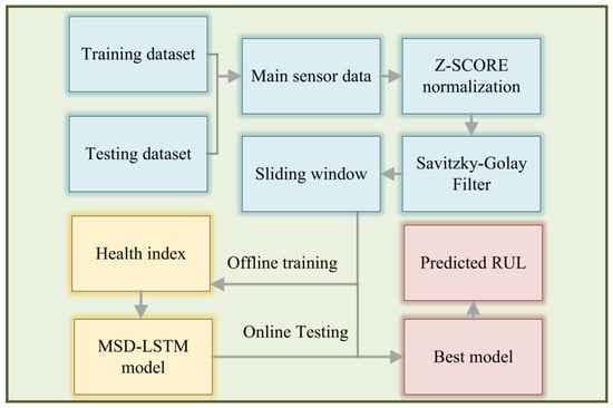
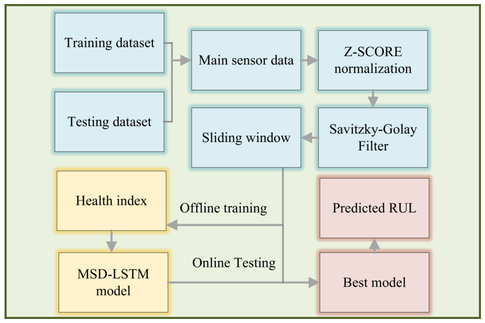
The proposed MSD-LSTM framework is designed around two principles that directly address the issues identified in Section 1: (i) hidden-state information produced by the LSTM should be exploited across the full input window rather than relying only on the final recurrent output, and (ii) attention-based temporal cues should be balanced with statistic-based window cues before being combined with deep features. Guided by these principles, the overall workflow is organized into an offline training stage and an online prediction stage, as illustrated in Figure 1.
Figure 1.
The overall process of the method for RUL prediction.
In the offline training stage, sensor channels with constant readings across the operational history are discarded, since they carry little degradation information and would otherwise inflate the input dimensionality. The remaining signals are standardized through z-score normalization, and a Savitzky–Golay (SG) filter is applied as an input-level smoothing step to attenuate high-frequency fluctuations while preserving the underlying degradation trend. A sliding-window scheme is then used to generate fixed-length samples, each paired with a piecewise-linear health-index label. In the online prediction stage, the trained model processes incoming sensor data in the same windowed form and outputs the corresponding RUL estimate. The sliding-window block in Figure 1 is therefore a data-segmentation operation rather than a trainable module: model parameters are learned only during offline training, whereas online prediction uses the fixed trained model and applies the same windowing rule to incoming sensor streams.
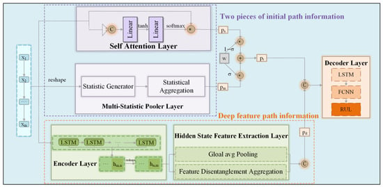
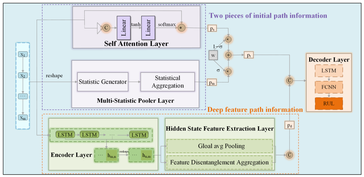
The internal structure of MSD-LSTM is composed of an LSTM encoder, a hidden-state feature extraction (HSFE) module, a Multi-Statistic Pooler (MSP), a self-attention branch, and an LSTM-based decoder, as illustrated in Figure 2. Within HSFE, a Feature Disentanglement Aggregation (FDA) sub-module and a Global Average Pooling (GAP) sub-module cooperate to extract local and global information from the LSTM hidden states. At a higher level, the framework operates along three complementary paths. The two auxiliary paths process the windowed signal in parallel: the self-attention branch emphasizes time steps that carry stronger degradation signatures, while the MSP summarizes the input window through multiple statistical indicators that are less sensitive to isolated local fluctuations. Their outputs are combined through a static-gating scheme, which forms the first-stage fusion and yields an initial feature representation that benefits from attention without being dominated by it. The deep path feeds the filtered signal through the LSTM encoder and then passes the hidden states to HSFE, producing a deep temporal representation that captures long-range degradation dynamics. The first-stage initial features and the deep features are then concatenated in a second-stage fusion, and the resulting representation is delivered to the LSTM-based decoder and a feed-forward network that jointly output the final RUL estimate.
Figure 2.
The framework of the proposed MSD-LSTM. The asterisk denotes the element-wise multiplication operator used in the feature-fusion path.
3.2. LSTM Encoder
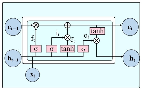
The deep path begins with an LSTM encoder that transforms the filtered sensor window into a sequence of hidden states, from which subsequent modules extract long-range degradation dynamics. The LSTM cell is chosen as the backbone of this path for two reasons. First, its gated memory structure, consisting of the forget gate, input gate and output gate, alleviates the vanishing- and exploding-gradient problems of conventional RNNs and is well suited to the multi-thousand-cycle sequences typical of aero-engine operation. Second, the intermediate hidden states produced by the gates are themselves informative temporal representations that can be reused by the downstream HSFE module introduced in Section 3.3, rather than being discarded after the final time step. The standard LSTM recurrence is given by Equations (1)–(6).
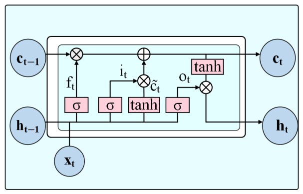
In these equations, denotes the output of the forget gate at time step t, represents the output of the input gate, is the candidate cell state, is the current cell state, denotes the output of the output gate, and is the hidden state at time step t. The parameters , , and , and , , , and are trainable weights and biases that are automatically updated through gradient-based optimization during training. The symbol denotes the sigmoid activation function, tanh represents the hyperbolic tangent function, and is the input sample at time step t. In Figure 3, also denotes the sigmoid gate activation rather than a standard-deviation operator. The hyperbolic tangent in Equation (3) is retained because it produces a bounded candidate state consistent with the conventional LSTM cell formulation, helping prevent the candidate memory update from introducing unbounded scale changes. The LSTM’s long-term memory cell update, as expressed in Equation (4), is determined jointly by the output of the forget gate , the previous cell state , the output of the input gate , and the candidate cell state ; this process combines the dual functions of forgetting and addition to generate the updated cell state, which in turn refreshes the hidden state . The overall structure of the LSTM unit is illustrated in Figure 3.
Figure 3.
LSTM unit.
The input sequence of the LSTM unit contains m time steps, where each vector has d retained sensor dimensions and m is determined by the sliding-window size. Denoting the encoder LSTM as the function , its input–output relationship can be expressed as shown in Equation (7), where the hidden-state sequence is produced by the final LSTM layer.
3.3. Hidden-State Feature Extraction Module
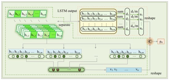
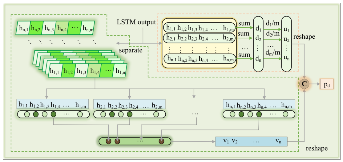
Conventional LSTM-based predictors feed only the final-step hidden state into the downstream regression head, implicitly assuming that all relevant temporal information has already been accumulated into that single vector. In long operational sequences, however, early-stage hidden states also carry distinctive degradation cues that tend to be diluted as information propagates along the LSTM chain. The HSFE module is designed to recover this under-utilized information through two cooperative sub-modules: a Feature Disentanglement Aggregation (FDA) branch and a Global Average Pooling (GAP) branch. The term “disentanglement” is used here in a feature-level engineering sense: FDA separates dimension-wise hidden-state cues for aggregation, but it does not claim a formal causal or generative disentanglement of the underlying degradation process. FDA operates along each hidden dimension independently and aggregates the entire sequence of hidden states through a set of learnable linear operations, so that dimension-wise salient cues can be sharpened rather than averaged out. GAP, in contrast, computes a dimension-wise average over the hidden-state sequence, which suppresses isolated fluctuations propagated along the LSTM chain and captures the stable, sequence-level component of the degradation pattern. The two branches therefore form a local–global cooperation: FDA preserves feature specificity while GAP enforces temporal stability. Their outputs are concatenated to form the deep feature , which is subsequently passed to the second-stage fusion. The mathematical formulations of HSFE are given by Equations (8)–(12).
In these equations, d and g denote the outputs of the Feature Disentanglement Aggregation (FDA) and Global avg Pooling (GAP) modules, respectively. Specifically, represents the computation result for the i-th dimension, obtained through a linear combination of m hidden states, where m corresponds to the sliding window size, while is derived from the mean value of m hidden states. The parameters and are trainable weights and biases that are automatically updated during the gradient-based optimization process. The overall architecture of the hidden-state feature extraction (HSFE) is illustrated in Figure 4.
Figure 4.
Hidden-state feature extraction layer.
The input to the Feature Disentanglement Aggregator is derived from the reshaped hidden cell states of the LSTM, denoted as , which represent the hidden cell states of the final LSTM layer. In this study, the number of LSTM layers is set to 2. The Feature Disentanglement Aggregator processes the hidden cell states and outputs for subsequent processing.
3.4. Self-Attention Branch
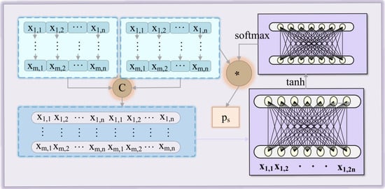
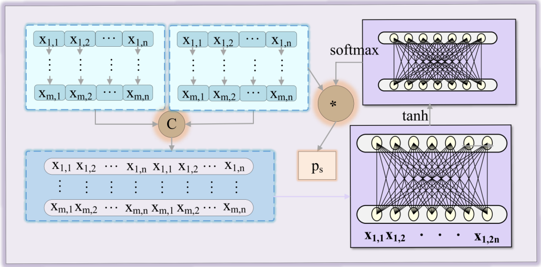
Although the deep path captures long-range degradation dynamics through the LSTM encoder, a portion of the raw-signal information inevitably fades as the sequence propagates along the recurrent chain. To preserve this initial information and complement the deep features, a self-attention branch is applied directly to the raw windowed signal rather than to the LSTM output. The branch re-weights the m time steps of the d-dimensional input according to their learned relevance, so that the time steps carrying stronger degradation signatures contribute more to the resulting representation. As illustrated in Figure 5, the input is first concatenated with itself and passed through two linear layers to compute the attention score s, which is then transformed into attention weights via a softmax operation. The initial feature representation is finally obtained by applying as time-step weights on the original input. The corresponding formulation is given by Equations (13)–(15).
Figure 5.
Self-attention layer. The asterisk denotes the weighted multiplication between the attention weights and the input time-step features.
3.5. Multi-Statistic Pooler and Static-Gating Fusion
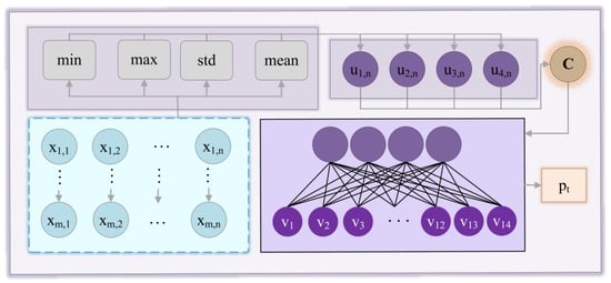
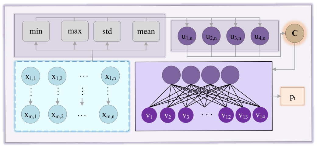
A self-attention branch alone may be sensitive to locally distinctive time steps, regardless of whether that distinctiveness stems from a genuine degradation event or from a short-term fluctuation. The Multi-Statistic Pooler (MSP) is therefore introduced as a complementary branch that summarizes window-level behavior. Instead of emphasizing specific time steps, MSP summarizes each sensor dimension of the raw window through four statistical indicators—minimum, maximum, standard deviation and mean—which jointly characterize the global trend and variability of the signal. The standard deviation is used as a descriptive indicator of within-window fluctuation strength rather than as evidence that the sensor values are Gaussian or symmetric. These indicators are then concatenated and passed through a linear projection to be mapped into a feature space that is compatible with the attention-based representation. Because the four indicators describe the window as a whole, the resulting feature provides a statistic-based counterpart to the attention output. MSP is not intended to replace sequential modeling; the temporal order and short-term dynamics are still modelled by the LSTM encoder and the HSFE branch, while MSP supplies an auxiliary window-level context. The corresponding formulation is given by Equations (16)–(20).
In Equations (16)–(20), i denotes a retained sensor dimension, where and . In addition, m represents the sample window size. The Multi-Statistic Pooler (MSP) concatenates multiple statistical indicators and maps them through a linear layer to obtain , which captures the overall trend of the data. The architecture of the MSP is illustrated in Figure 6.
Figure 6.
Multi-Statistic Pooler layer.
Given the two complementary branches, a naive concatenation or element-wise addition would treat the attention-based and statistics-based cues as equally weighted, which either under-uses the more informative one or allows the less reliable one to dominate the representation. To balance the two cues in a data-adaptive manner, the first-stage fusion is implemented as a static-gating operation, whose gating coefficient is a trainable scalar optimized end-to-end with the rest of the network. The fused output is then passed to the second-stage fusion together with the deep feature produced by the HSFE module. The gating operation is formulated as Equation (21).
In these equations, represents the output variable from the Multi-Statistic Pooler (MSP), denotes the output variable from the self-attention mechanism, is the sigmoid activation function, w is the trainable parameter optimized by the model, and is the output of the static-gating mechanism, which provides enriched initial feature representations.
3.6. Decoder and RUL Regression Head
After the two-stage fusion, the resulting representation encodes degradation information from three cooperating paths but is still a concatenated high-dimensional vector. A decoder is therefore used to process this fused representation before mapping it to a scalar health-index value. Following the encoder–decoder design widely adopted in sequence-to-sequence modeling, the decoder here consists of an LSTM block followed by a fully connected regression head. The decoder LSTM uses the same depth and hidden size as the encoder LSTM and is initialized with the final hidden and cell states of the encoder, so the fused representation is decoded with temporal state information inherited from the encoder. The decoder output is given by Equation (22).
In this equation, denotes the processing function of the decoder LSTM, denotes the final hidden and cell states passed from the encoder to initialize the decoder, denotes the first-stage fused feature from the initial-information path, and denotes the deep feature produced by the HSFE module. The output is the predicted normalized health index.
4. Experimental Setup and Results
4.1. Dataset Description
The proposed MSD-LSTM is evaluated on the Commercial Modular Aero-Propulsion System Simulation (C-MAPSS) turbofan engine degradation dataset released by NASA [41], which has become a de facto benchmark for data-driven aero-engine RUL prediction. The dataset simulates run-to-failure trajectories under a range of operating conditions and fault modes, and thus allows an assessment of predictive accuracy under different condition and fault settings. As summarized in Table 1, the benchmark consists of four sub-datasets (FD001–FD004) with increasing complexity: FD001 and FD003 involve a single operating condition, while FD002 and FD004 span six operating conditions; in parallel, FD003 and FD004 additionally include two concurrent fault modes. Each record contains 26 dimensions, comprising the unit identifier, operating cycle count, three operational settings (altitude, Mach number and throttle resolver angle) and 21 sensor measurements that capture temperature, pressure, rotational speed and related thermodynamic variables. Every sub-dataset is partitioned into a training set, in which engines run from a healthy state to failure, and a testing set, in which sequences are truncated at some point prior to failure so that the ground-truth RUL can be used to evaluate the model.
Table 1.
Description of the C-MAPSS dataset.
4.2. Data Preprocessing
4.2.1. Sensor Selection
Each sub-dataset of C-MAPSS contains 21 sensor channels, among which seven remain constant throughout the operational cycles and therefore carry no degradation information. Following the sensor selection protocol commonly adopted in the literature [42], channels numbered 1, 5, 6, 10, 16, 18 and 19 are discarded, and the remaining 14 channels are retained as model input.
4.2.2. Data Normalization
The 14 retained sensors measure physically distinct quantities with markedly different magnitudes and units. Feeding such heterogeneous values directly into a neural network would cause sensors with larger magnitudes to dominate the gradient updates, while those with smaller magnitudes contribute little to the learned representation. To place all sensor dimensions on a comparable scale and stabilize training, Z-score normalization is applied as formulated in Equation (23).
In this formula, represents the normalized value of the q-th feature dimension for the p-th sample, is the original value of that feature, denotes the mean of the q-th feature dimension, and represents its standard deviation. Here, the standard deviation is used only for scale normalization of each retained sensor channel; no Gaussian or symmetry assumption on the sensor distribution is required.
4.2.3. Filtering Process
Sensor sequences used for RUL prediction commonly contain local fluctuations that can weaken the quality of recurrent hidden-state features. The Savitzky–Golay (SG) filter is therefore applied as an input-level smoothing step, as it attenuates high-frequency fluctuations while preserving the low-frequency degradation trend that is essential for RUL estimation. Within a local SG window, the filter fits a polynomial of order k by minimizing the sum of squared residuals, and the optimal coefficients are obtained by setting the partial derivatives of the squared error with respect to each coefficient to zero, yielding a closed-form linear system.
Specifically, the polynomial fitting function within the window is expressed in Equation (24), and after derivation and simplification, the resulting linear system is shown in Equation (25). The coefficient of the fitted polynomial represents the final corrected value of the window’s central point, as described in Equation (26).
In Equation (26), denotes the final corrected value. In Equation (24), represents the k-th order coefficient of the fitted polynomial, where k is a predefined fitting parameter, and t indicates the position index relative to the center of the SG window. In Equation (25), p refers to the index of the coefficient for which the partial derivative is computed, with . The parameter ℓ denotes the half-width of the SG window, and represents the original data value corresponding to position t.
4.2.4. Piecewise Linear RUL Modeling
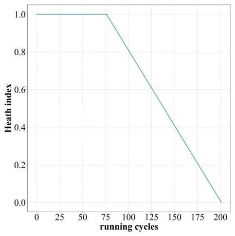
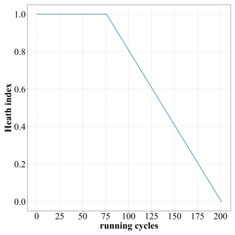
During the early phase of engine operation, performance remains relatively stable and the actual degradation is negligible, whereas clear degradation is observed only after a certain number of cycles. Treating RUL as linearly decreasing from the very first cycle would therefore force the model to fit a non-existent trend in the healthy phase and dilute the learning signal associated with the actual degradation phase. Following the widely adopted piecewise-linear RUL convention [43,44], a health-index (HI) label is constructed as in Equation (27), in which RUL is held at its upper bound during the healthy phase and decreases linearly thereafter.
In this equation, denotes the health index of the k-th engine, H represents the modeled value of the maximum remaining useful life (RUL) during the engine’s initial stable operation stage, which is set to 125 operating cycles [45]. refers to the total number of operating cycles for the k-th engine, and denotes its dynamic operating cycle count. The health index is constructed as a piecewise function. As an illustrative example, Figure 7 presents the RUL modeling result for Engine No. 66.
Figure 7.
Health-index model.
4.2.5. Sliding Window
To provide the model with fixed-length temporal inputs, a sliding-window scheme [26] is applied to each engine’s sensor sequence , where n is the sequence length and d is the number of retained sensor dimensions. A window of length m is slid along the time axis with a stride of one, producing the sample sequence that serves as the model input. When the full sequence length n of a testing engine is shorter than the window size m, cubic spline interpolation is applied to pad the missing time steps.
4.3. Experimental Setup and Evaluation Metrics
4.3.1. Experimental Setup
The model is trained end-to-end by minimizing the mean squared error between the predicted and ground-truth health indices, as defined in Equation (28). The parameters are updated through back-propagation using the RMSprop optimizer with a batch size of 128, an initial learning rate of 0.002, and a weight decay of . A step learning-rate scheduler is used during training. The single-condition sub-datasets FD001 and FD003 use the same window-related setting, while the multi-condition sub-datasets FD002 and FD004 use a longer input window to accommodate their more complex operating profiles. The RUL upper bound is set to 125 cycles for all four sub-datasets. All modules, including the LSTM encoder, the HSFE branch, the self-attention and MSP branches, the static gate, and the LSTM-based decoder, are jointly optimized under the same objective. All comparative results follow the official C-MAPSS train/test partitions. Conventional random k-fold cross-validation is not applied because each engine trajectory is an ordered run-to-failure sequence and random reassignment of windows would mix temporal segments from the same degradation process across folds.
4.3.2. Evaluation Metrics
Two metrics widely adopted in the C-MAPSS literature [46] are used to evaluate predictive performance: the Root Mean Square Error (RMSE) and the SCORE function. RMSE, defined in Equation (29), symmetrically measures the magnitude of the prediction error and thus reflects overall accuracy. SCORE, defined in Equation (30), is instead asymmetric and is specifically designed for safety-critical prognostics: predictions made later than the true failure time (i.e., overestimated RUL) are penalized more heavily than predictions made earlier. This asymmetry reflects the engineering reality that, in aero-engine maintenance, an optimistic RUL estimate that delays necessary replacement is far more costly than a conservative estimate that triggers slightly early maintenance. SCORE is therefore regarded as the more engineering-relevant indicator, and is emphasized in the subsequent analysis.
In these equations, M represents the number of engines, and denotes the difference between the predicted and actual RUL of the i-th testing engine. The model is trained on capped and normalized health-index labels, while RMSE and SCORE are calculated after rescaling the predictions back to RUL cycles. As shown in Equation (30), when , meaning the prediction is earlier than the actual failure time, the SCORE function applies a smaller penalty. Conversely, when , indicating a late prediction, a larger penalty is imposed.
4.4. Hyperparameter Tuning Experiments
This section investigates how the main architectural and filtering hyperparameters affect the predictive performance of MSD-LSTM. The detailed parameter study is reported on FD001, which is a common single-condition C-MAPSS benchmark. The selected architecture-level settings, including the LSTM depth, hidden size, and static-gate initialization, are then kept fixed in the subsequent experiments, while window-related settings follow the complexity of the corresponding sub-dataset group.
4.4.1. Model Network Parameter Analysis
Four hyperparameters are tuned at the architectural level: the number of LSTM layers in the encoder–decoder pair (), the number of hidden units in each LSTM layer (), the initial value of the static-gating scalar (), and the number of hidden units in the self-attention branch (). The encoder and decoder LSTMs use the same values of and . Each hyperparameter is tuned independently while the others are fixed at their default values.
The tuning results for and are summarized in Table 2. With the hidden size fixed, varying from Configuration 1 to Configuration 6 shows that RMSE first decreases and then increases, reaching its minimum at ; deeper stacks bring no further benefit on this sequence-regression task. With fixed at two, Configurations 7–11 show a similar pattern for , with RMSE minimized at . The static-gate initializer and the self-attention hidden size are tuned under the same protocol, yielding and for the FD001 setting. The configuration used in the FD001 parameter study is listed in Table 3.
Table 2.
LSTM hyperparameter study.
Table 3.
Configuration used in the FD001 parameter study.
4.4.2. Savitzky–Golay Filter Parameter Study
Since the SG filter is introduced to smooth local signal fluctuations before they propagate through the LSTM chain, its two hyperparameters—the window length and the polynomial order—directly shape the trade-off between fluctuation attenuation and trend preservation. A grid search is therefore conducted on FD001 over their joint configuration space.
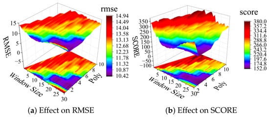
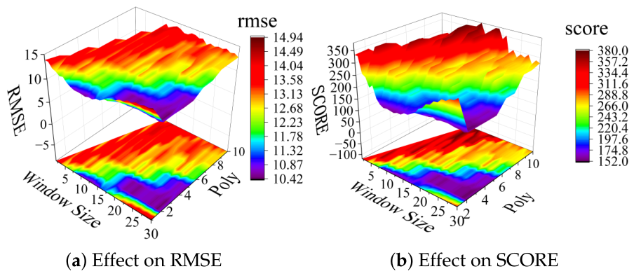
Figure 8 reports the joint effect of the window length and polynomial order across 245 combinations on FD001. Both metrics exhibit a clear interaction between the two hyperparameters: the best performance is obtained with a relatively large window size paired with a low polynomial order, which corresponds to stronger fluctuation attenuation while retaining a smooth low-order approximation of the degradation trend. Small windows provide limited smoothing, while high-order polynomials tend to over-fit residual fluctuations. The best FD001 combination is a window length of 29 and a polynomial order of 2. Figure 8 also provides an empirical view of the filtering effect because poor parameter combinations lead to clear RMSE and SCORE degradation. To further check the contribution of the SG step itself, the FD001 setting is evaluated once without pre-filtering under the same model configuration; RMSE and SCORE increase from 10.45 to 13.76 and from 149.45 to 332.71, respectively. This gap supports the usefulness of input-level smoothing in the proposed framework.
Figure 8.
Effect of Savitzky–Golay filtering parameters on model performance.
4.4.3. Study on the Two-Stage Fusion Mechanism
The MSD-LSTM produces three complementary feature streams—the self-attention output , the MSP output , and the HSFE deep feature —that must be combined before being passed to the decoder. Direct concatenation increases the feature dimension, whereas element-wise addition forces the streams to have equal weights. The proposed fusion therefore proceeds in two stages. The first stage handles the two initial-information streams: and are fused through the static-gating mechanism introduced in Section 3.5, so that the attention-based and statistics-based cues are balanced before downstream processing. The second stage then concatenates the gated initial feature with the deep feature , forming a compact representation that combines window-level information with hidden-state features.
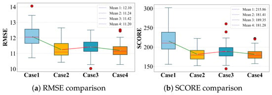
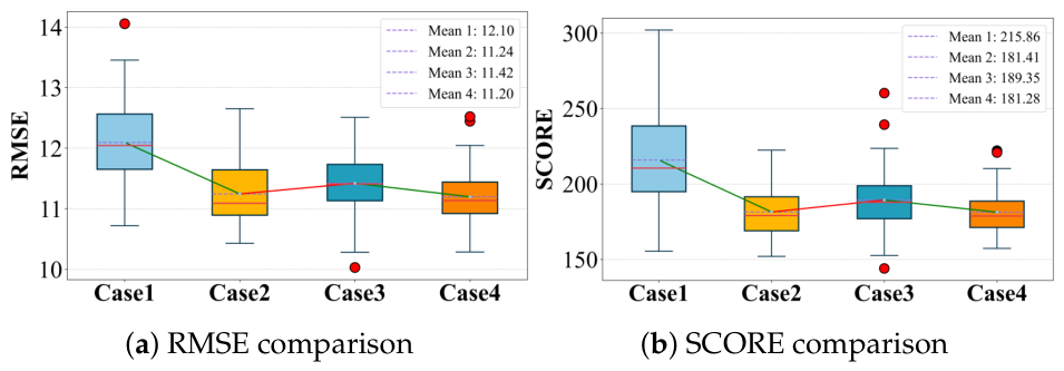
To evaluate the proposed fusion design, four alternative schemes are compared on FD001, as listed in Table 4: dot-product fusion, concatenation, element-wise addition, and the proposed two-stage fusion. Each scheme is independently trained and evaluated 100 times to reduce the effect of random initialization, and the resulting RMSE and SCORE distributions are visualized in Figure 9, where the red line inside each box denotes the median. Dot-product fusion yields consistently high RMSE and SCORE values. Concatenation and element-wise addition achieve lower medians, but both produce noticeable outliers on the SCORE metric. In contrast, the proposed two-stage fusion gives low median values on both metrics and shows a more stable distribution across repeated runs. This result supports the use of the two-stage fusion in the subsequent experiments.
Table 4.
Feature fusion methods.
Figure 9.
Evaluation of feature fusion methods. Red lines indicate median values, and circles indicate outliers in the boxplots.
4.5. Comparative Experiments
4.5.1. Visualization of RUL Prediction Results
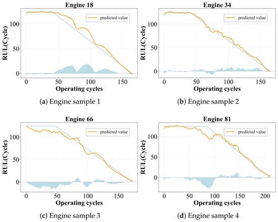
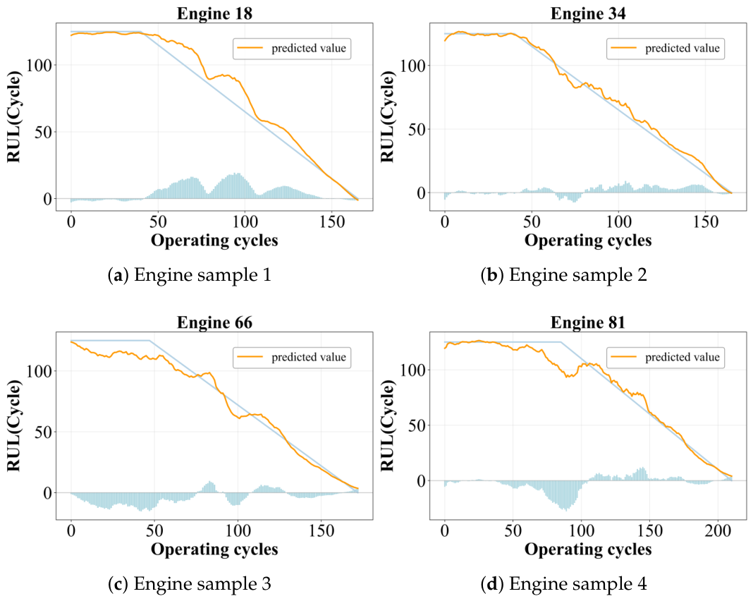
To qualitatively examine the behaviour of MSD-LSTM, four engines are randomly selected from the test set and their predicted RUL trajectories are visualized in Figure 10. Two patterns are observed across the four cases. During the early, healthy phase of each engine, the predicted RUL oscillates mildly around the piecewise-linear upper bound, where degradation-related sensor changes are limited. As the engine enters the degradation phase, the predictions move closer to the true RUL trajectory and the residuals become smaller. This trend is relevant to condition-based maintenance because prediction near the degradation phase has a direct effect on replacement timing.
Figure 10.
Predicted remaining useful life for randomly selected engine unit samples. The orange line denotes the predicted RUL trajectory, the blue line denotes the true RUL trajectory, and the bars denote the prediction error, calculated as predicted RUL minus true RUL.
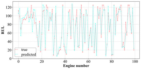
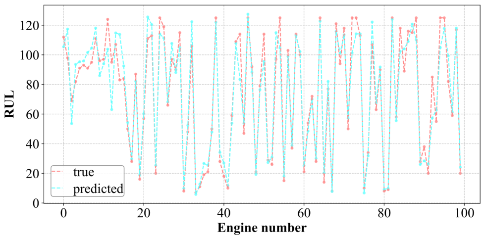
Figure 11 further presents the prediction results over all 100 engines of FD001, where the horizontal axis denotes the engine index and the vertical axis denotes the corresponding RUL value. The predicted curve tracks the ground-truth curve closely across nearly all engines, which shows that the accuracy observed on the four randomly sampled cases above is representative rather than incidental.
Figure 11.
RUL prediction result of FD001.
4.5.2. Comparison with Recent Methods
Table 5 reports the quantitative comparison between MSD-LSTM and fifteen recent methods across the four C-MAPSS sub-datasets (“N/A” denotes values not disclosed in the original publication). The compared methods include knowledge-guided networks, attention-based deep networks, Transformer-based predictors, hybrid spatial–temporal frameworks, and graph-structured predictors, forming a representative cross-section of recent C-MAPSS RUL studies.
Table 5.
Comparison of different models.
On the single-condition sub-datasets FD001 and FD003, MSD-LSTM achieves the lowest RMSE and the lowest or near-lowest SCORE among the compared methods. On FD002, which involves six operating conditions and is considerably more challenging than FD001, MSD-LSTM attains both the best RMSE and the best SCORE in the comparison table, indicating that the proposed design remains effective under more complex operating conditions. On the most challenging sub-dataset FD004—which combines six operating conditions with two concurrent fault modes—MambAtt attains a lower RMSE, whereas MSD-LSTM achieves a lower SCORE. Given that SCORE penalizes overestimated RUL more heavily than underestimated RUL, this outcome suggests fewer late-prediction errors on FD004, even though the symmetric error is larger.
Taken across all four sub-datasets, MSD-LSTM provides a balanced result: it remains close to the best-performing method on RMSE while showing consistent competitiveness on SCORE. Several baselines achieve strong results on one metric or one sub-dataset but fall behind on others, whereas MSD-LSTM maintains comparatively stable performance across the benchmark. These results support the usefulness of combining hidden-state extraction with statistic-guided fusion for C-MAPSS aero-engine RUL prediction.
4.6. Ablation Experiments
This section quantifies the contribution of the two dedicated modules proposed in this paper—HSFE and MSP—through ablation experiments, and further visualizes the feature maps produced by MSP and the self-attention branch to examine whether they capture complementary aspects of the degradation process.
4.6.1. Ablation Study of Model Components
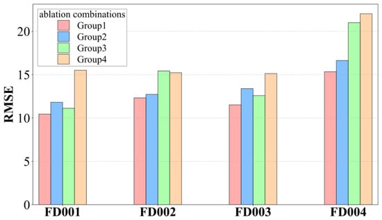
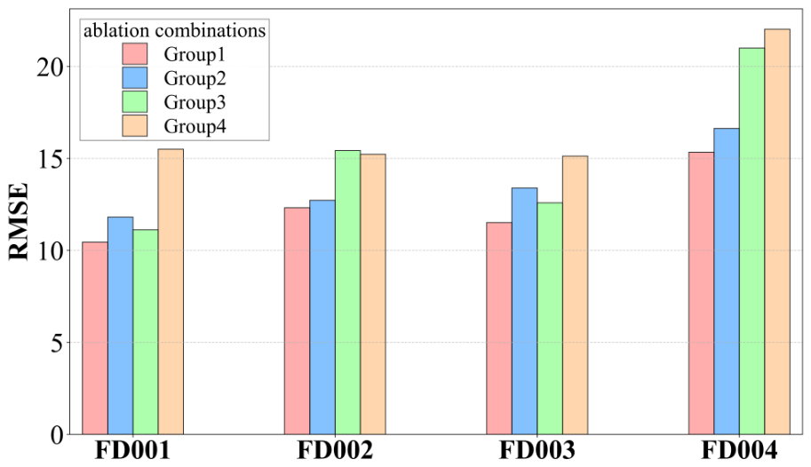
Four variants are constructed to isolate the contribution of each proposed module: Group 1 is the full MSD-LSTM with both MSP and HSFE; Group 2 removes the MSP branch while retaining HSFE; Group 3 removes the HSFE module while retaining MSP; and Group 4 removes both, leaving only the LSTM encoder together with the self-attention branch. All four variants are trained and evaluated on the four C-MAPSS sub-datasets using the corresponding experimental settings for each sub-dataset, and the resulting RMSE values are presented in Figure 12. The ablation comparison uses the same official test set and evaluation protocol as Table 5; therefore, Figure 12 should be interpreted as a controlled component-level comparison rather than a cross-validation plot with error bars.
Figure 12.
Ablation study results on four datasets.
The ablation results support three points. First, both Group 2 and Group 3 outperform Group 4 on every sub-dataset, which indicates that MSP and HSFE each bring an independent improvement when added on top of the baseline backbone. Second, Group 3 (no HSFE) consistently performs worse than Group 2 (no MSP) on the more complex sub-datasets FD002 and FD004, suggesting that hidden-state utilization becomes more important when the operating conditions and fault modes are more complex. Third, Group 1 (the full model) achieves the lowest RMSE on all four sub-datasets, indicating that the two modules work best when used together: HSFE supplies the deep path with hidden-state representations, while MSP provides a statistic-based auxiliary representation for the attention branch. The ablation therefore supports the coupled design of MSD-LSTM.
4.6.2. Feature Visualization
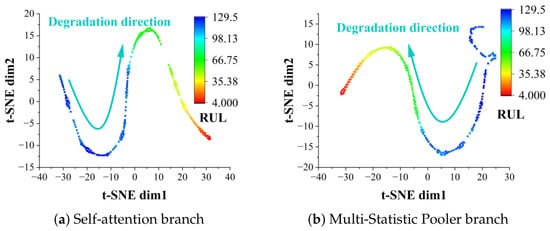
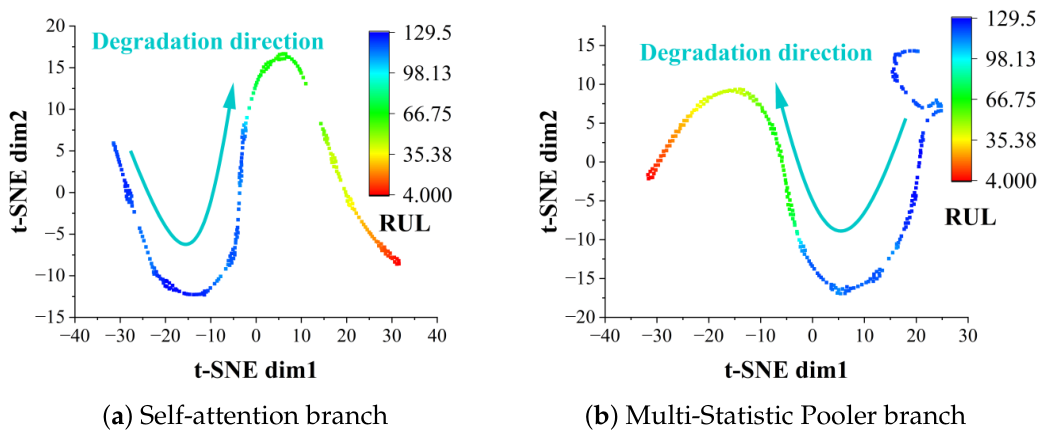
To examine whether MSP and the self-attention branch indeed play complementary roles, their output feature maps on a representative test engine (Engine No. 94) are projected into two dimensions via t-distributed Stochastic Neighbor Embedding (t-SNE) [57]. Figure 13 shows the resulting 2D embeddings, with color encoding the ground-truth RUL.
Figure 13.
Visualization of learned features.
The two embeddings exhibit distinct geometries. The self-attention branch concentrates late-stage samples on the right portion of the manifold, which is consistent with its learned tendency to place high weights on time steps carrying strong degradation signatures. The MSP branch shows a different pattern, spreading early-stage samples more evenly and retaining a smoother trajectory across the full RUL range. This matches the design intuition that window-level statistics preserve global trend information. The two feature spaces therefore appear to provide complementary views rather than rescaled versions of the same representation. The visualization is consistent with the quantitative ablation results and with the combined use of MSP and self-attention through static-gating fusion.
Overall, the ablation and visualization results are consistent with the MSD-LSTM design. HSFE and MSP are each individually effective, and their combination produces a larger improvement than either module alone. Meanwhile, the self-attention branch and the MSP branch, although both operating on the input window, learn representations with distinct spatial characteristics. This observation is consistent with the intended role of the static-gating fusion: attention emphasizes locally informative timestamps, whereas MSP preserves window-level statistical trends.
5. Discussion
The experimental results indicate that MSD-LSTM benefits from combining recurrent hidden-state modeling with statistic-guided auxiliary features. On the more complex FD002 and FD004 sub-datasets, where multiple operating conditions and fault modes increase the variability of the sensor trajectories, the HSFE module is particularly useful because it extracts information from the full sequence of LSTM hidden states instead of relying on a single terminal state. This behavior is consistent with the motivation that different portions of a sliding window may encode complementary degradation cues.
The MSP branch provides a different type of information from the self-attention branch. Attention assigns weights to time steps according to learned relevance, which is helpful for locating degradation-sensitive segments but can also react to local fluctuations. By contrast, MSP describes each input window through minimum, maximum, standard deviation, and mean statistics. These descriptors are simple, but they summarize the overall level and variability of the window and therefore provide a stable counterpart to attention-based features. The fusion experiments further show that this combination is preferable to direct concatenation, addition, or dot-product fusion under the tested FD001 setting.
Compared with recent RNN–LSTM, CNN–LSTM, statistics-aware, and attention-based RUL studies, MSD-LSTM differs in where the statistical information is used. Earlier turbofan-engine studies have shown the usefulness of recurrent-model combination and LSTM-attention modeling on C-MAPSS data [15,16]. PALC-Net uses partial convolution with an attention-enhanced CNN–LSTM structure to reduce computational overhead while preserving prediction accuracy [17], while a deep equilibrium model estimates aircraft-engine RUL through implicit spatiotemporal representation and calibrated Monte Carlo dropout [18]. Related equipment RUL studies have also explored gated feature fusion in deep prognostic models [19]. The LSTM-MSAA method enriches attention scores with matrix-level descriptors such as the Frobenius norm, spectral norm, and soft rank [20], while the MDFA model uses multi-scale dilated convolution and fusion attention to capture degradation patterns at different temporal scales [21]. In MSD-LSTM, the statistic-based representation is kept as an MSP branch and fused with attention through static gating; the resulting auxiliary representation is then combined with hidden-state features extracted by HSFE. The method therefore uses statistics as a separate feature path rather than only as an attention-score modifier, an implicit temporal representation, or a multi-scale convolutional cue.
Several limitations should be noted. First, all experiments are conducted on the simulated C-MAPSS benchmark. Although C-MAPSS is widely used for aero-engine RUL evaluation, it cannot fully represent sensor drift, maintenance interventions, and unforeseen operating regimes in in-service engines. Second, the current study does not include N-CMAPSS or other cross-domain validation datasets, so generalization beyond C-MAPSS remains to be further examined. Third, the SG filter and static-gating scalar are fixed according to the current experimental protocol, and adaptive filtering or condition-aware gating may further improve robustness. In particular, the present model is trained offline and then used for inference with fixed parameters; it does not yet include online updating for concept drift under changing operational regimes. Finally, the multi-path representation improves prediction performance, but additional interpretability analysis would be needed before using the model as a diagnostic-support tool. The proposed feature-level disentanglement should also be interpreted as an empirical representation strategy rather than as a mathematically formal separation of the data-generating degradation process.
6. Conclusions
This paper has presented MSD-LSTM, a multi-path framework for aero-engine remaining useful life prediction. The framework combines SG input smoothing, an HSFE module for exploiting LSTM hidden-state sequences, an MSP branch for statistic-based window representation, a self-attention branch for local temporal relevance, and static-gating fusion for combining auxiliary features. Experiments on the NASA C-MAPSS benchmark show that MSD-LSTM obtains lower or comparable RMSE and SCORE values across the four sub-datasets compared with recent methods. The ablation, fusion, and visualization analyses show that HSFE and MSP make complementary contributions to the final prediction. The implemented model contains approximately 5.58 k trainable parameters, and the inference stage requires only window construction followed by a forward pass through the trained network. Although no embedded-hardware or real-time onboard test has been conducted in this study, this compact parameter scale suggests that hardware-oriented deployment is a feasible direction for subsequent validation.
Future work will consider validation on more realistic degradation datasets, transfer- or domain-adaptation extensions, online updating under concept drift, hardware-in-the-loop testing, and additional interpretability analysis for maintenance decision support.
Author Contributions
Conceptualization, L.Z. and Q.L.; methodology, L.Z., T.W. and Q.L.; software, L.Z.; validation, L.Z., H.X. and P.Z.; formal analysis, L.Z. and T.W.; investigation, T.W. and Y.L.; resources, T.W. and Q.L.; data curation, L.Z.; writing—original draft preparation, L.Z.; writing—review and editing, L.Z., T.W. and Q.L.; visualization, L.Z.; supervision, Q.L.; project administration, Q.L.; funding acquisition, Q.L. All authors have read and agreed to the published version of the manuscript.
Funding
This research was funded by the National Key R&D Program of China, grant number 2023YFB4302400.
Institutional Review Board Statement
Not applicable.
Informed Consent Statement
Not applicable.
Data Availability Statement
The C-MAPSS dataset analyzed in this study is publicly available from the NASA Prognostics Center of Excellence data repository (https://www.nasa.gov/intelligent-systems-division/discovery-and-systems-health/pcoe/pcoe-data-set-repository/, accessed on 26 June 2026). The implementation code is available from the corresponding author upon reasonable request.
Conflicts of Interest
Lishun Zhang is affiliated with Xihua University and Civil Aviation Electronic Technology Co., Ltd. Tao Wen, Huan Xia, Ping Zhang, and Youyang Li are affiliated with Civil Aviation Second Research Institute Co., Ltd. and Civil Aviation Electronic Technology Co., Ltd. Qian Luo is affiliated with Xihua University, Civil Aviation Second Research Institute Co., Ltd., and Civil Aviation Electronic Technology Co., Ltd., as indicated in the manuscript. Apart from the authors’ institutional affiliations and normal research duties, the funder and affiliated institutions/companies had no additional role in the design of the study; in the collection, analyses, or interpretation of data; in the writing of the manuscript; or in the decision to publish the results. The authors declare that there are no other financial or non-financial conflicts of interest related to the work under consideration.
References
- Jiang, F.; Hou, X.; Xia, M. Spatio-temporal attention-based hidden physics-informed neural network for remaining useful life prediction. Adv. Eng. Inform. 2025, 63, 102958. [Google Scholar] [CrossRef] [Scilit]
- Zhou, Y.; Wang, H.; Jin, H.; Liu, Y.; Liu, X.; Cao, Z. Remaining useful life prediction for machinery using multimodal interactive attention spatial-temporal networks with deep ensembles. Expert Syst. Appl. 2025, 263, 125808. [Google Scholar] [CrossRef] [Scilit]
- Wei, Z.; Zhao, Z.; Zhou, Z.; Yan, R. Collaborative-sequential optimization for aero-engine maintenance based on multi-agent reinforcement learning. Expert Syst. Appl. 2024, 247, 123358. [Google Scholar] [CrossRef] [Scilit]
- Cai, X.; Li, N.; Xie, M. RUL prediction for two-phase degrading systems considering physical damage observations. Reliab. Eng. Syst. Saf. 2024, 244, 109926. [Google Scholar] [CrossRef] [Scilit]
- Yin, C.; Li, Y.; Wang, Y.; Dong, Y. Physics-guided degradation trajectory modeling for remaining useful life prediction of rolling bearings. Mech. Syst. Signal Process. 2025, 224, 112192. [Google Scholar] [CrossRef] [Scilit]
- Liang, J.; Liu, H.; Xiao, N.C. A hybrid approach based on deep neural network and double exponential model for remaining useful life prediction. Expert Syst. Appl. 2024, 249, 123563. [Google Scholar] [CrossRef] [Scilit]
- Hochreiter, S.; Schmidhuber, J. Long Short-Term Memory. Neural Comput. 1997, 9, 1735–1780. [Google Scholar] [CrossRef] [Scilit] [PubMed]
- Boujamza, A.; Lissane Elhaq, S. Attention-based LSTM for Remaining Useful Life Estimation of Aircraft Engines. IFAC-PapersOnLine 2022, 55, 450–455. [Google Scholar] [CrossRef] [Scilit]
- Shi, J.; Zhong, J.; Zhang, Y.; Xiao, B.; Xiao, L.; Zheng, Y. A dual attention LSTM lightweight model based on exponential smoothing for remaining useful life prediction. Reliab. Eng. Syst. Saf. 2024, 243, 109821. [Google Scholar] [CrossRef] [Scilit]
- Park, Y.I.; Kang, S.J. Query-Vector-Focused Recurrent Attention for Remaining Useful Life Prediction. IEEE Trans. Reliab. 2025, 74, 5564–5578. [Google Scholar] [CrossRef] [Scilit]
- Fu, S.; Jia, Y.; Lin, L.; Suo, S.; Guo, F.; Zhang, S.; Liu, Y. PSTFormer: A novel parallel spatial-temporal transformer for remaining useful life prediction of aeroengine. Expert Syst. Appl. 2025, 265, 125995. [Google Scholar] [CrossRef] [Scilit]
- Zhang, Q.; Liu, J.; Xie, K.; Liu, Q. A dynamic spatio-temporal graph neural network with global and local perception for remaining useful life prediction. Expert Syst. Appl. 2025, 282, 127707. [Google Scholar] [CrossRef] [Scilit]
- Gelman, L.M.; Kripak, D.A.; Fedorov, V.V.; Udovenko, L.N. Condition Monitoring Diagnosis Methods of Helicopter Units. Mech. Syst. Signal Process. 2000, 14, 613–624. [Google Scholar] [CrossRef] [Scilit]
- Lin, D.Y.; Wu, C.C. Multi-stage Stochastic Engine Usage Optimization for Fighter Jet Fleet Using Nested Decomposition Algorithm. Oper. Res. Perspect. 2026, 14, 100376. [Google Scholar] [CrossRef] [Scilit]
- Chui, K.T.; Gupta, B.B.; Vasant, P. A Genetic Algorithm Optimized RNN-LSTM Model for Remaining Useful Life Prediction of Turbofan Engine. Electronics 2021, 10, 285. [Google Scholar] [CrossRef] [Scilit]
- Muneer, A.; Taib, S.M.; Naseer, S.; Ali, R.F.; Aziz, I.A. Data-Driven Deep Learning-Based Attention Mechanism for Remaining Useful Life Prediction: Case Study Application to Turbofan Engine Analysis. Electronics 2021, 10, 2453. [Google Scholar] [CrossRef] [Scilit]
- Wu, L.; Song, S.; Li, H.; Hu, C.; Luo, Y. PALC-Net: A Partial Convolution Attention-Enhanced CNN-LSTM Network for Aircraft Engine Remaining Useful Life Prediction. Electronics 2026, 15, 131. [Google Scholar] [CrossRef] [Scilit]
- Plakias, S.; Boutalis, Y.S. A Deep Equilibrium Model for Remaining Useful Life Estimation of Aircraft Engines. Electronics 2025, 14, 2355. [Google Scholar] [CrossRef] [Scilit]
- Cui, H.; Guo, X.; Yu, L. Leveraging Pre-Trained GPT Models for Equipment Remaining Useful Life Prognostics. Electronics 2025, 14, 1265. [Google Scholar] [CrossRef] [Scilit]
- Hatipoğlu, A.; Yılmaz, E. A Matrix-Statistics-Aware Attention Mechanism for Robust RUL Estimation in Aero-Engines. Appl. Sci. 2026, 16, 169. [Google Scholar] [CrossRef] [Scilit]
- Xiao, G.; Jin, C.; Bai, J. Remaining Useful Life Prediction for Aero-Engines Based on Multi-Scale Dilated Fusion Attention Model. Appl. Sci. 2025, 15, 9813. [Google Scholar] [CrossRef] [Scilit]
- Chen, J.; Jing, H.; Chang, Y.; Liu, Q. Gated recurrent unit based recurrent neural network for remaining useful life prediction of nonlinear deterioration process. Reliab. Eng. Syst. Saf. 2019, 185, 372–382. [Google Scholar] [CrossRef] [Scilit]
- Song, T.; Liu, C.; Wu, R.; Jin, Y.; Jiang, D. A hierarchical scheme for remaining useful life prediction with long short-term memory networks. Neurocomputing 2022, 487, 22–33. [Google Scholar] [CrossRef] [Scilit]
- Zhang, J.; Wang, P.; Yan, R.; Gao, R.X. Long short-term memory for machine remaining life prediction. Spec. Issue Smart Manuf. 2018, 48, 78–86. [Google Scholar] [CrossRef] [Scilit]
- Ragab, M.; Chen, Z.; Wu, M.; Kwoh, C.K.; Yan, R.; Li, X. Attention-based sequence to sequence model for machine remaining useful life prediction. Neurocomputing 2021, 466, 58–68. [Google Scholar] [CrossRef] [Scilit]
- Liu, H.; Liu, Z.; Jia, W.; Lin, X. Remaining Useful Life Prediction Using a Novel Feature-Attention-Based End-to-End Approach. IEEE Trans. Ind. Inform. 2021, 17, 1197–1207. [Google Scholar] [CrossRef] [Scilit]
- Tseng, S.H.; Tran, K.D. Predicting maintenance through an attention long short-term memory projected model. J. Intell. Manuf. 2024, 35, 807–824. [Google Scholar] [CrossRef] [Scilit]
- Xiang, F.; Zhang, Y.; Zhang, S.; Wang, Z.; Qiu, L.; Choi, J.H. Bayesian gated-transformer model for risk-aware prediction of aero-engine remaining useful life. Expert Syst. Appl. 2024, 238, 121859. [Google Scholar] [CrossRef] [Scilit]
- Bai, R.; Noman, K.; Yang, Y.; Li, Y.; Guo, W. Towards trustworthy remaining useful life prediction through multi-source information fusion and a novel LSTM-DAU model. Reliab. Eng. Syst. Saf. 2024, 245, 110047. [Google Scholar] [CrossRef] [Scilit]
- Ayodeji, A.; Wang, Z.; Wang, W.; Qin, W.; Yang, C.; Xu, S.; Liu, X. Causal augmented ConvNet: A temporal memory dilated convolution model for long-sequence time series prediction. ISA Trans. 2022, 123, 200–217. [Google Scholar] [CrossRef] [Scilit] [PubMed]
- Zhang, Q.; Liu, Q.; Ye, Q. An attention-based temporal convolutional network method for predicting remaining useful life of aero-engine. Eng. Appl. Artif. Intell. 2024, 127, 107241. [Google Scholar] [CrossRef] [Scilit]
- Cao, Y.; Ding, Y.; Jia, M.; Tian, R. A novel temporal convolutional network with residual self-attention mechanism for remaining useful life prediction of rolling bearings. Reliab. Eng. Syst. Saf. 2021, 215, 107813. [Google Scholar] [CrossRef] [Scilit]
- Lin, L.; Wu, J.; Fu, S.; Zhang, S.; Tong, C.; Zu, L. Channel attention & temporal attention based temporal convolutional network: A dual attention framework for remaining useful life prediction of the aircraft engines. Adv. Eng. Inform. 2024, 60, 102372. [Google Scholar] [CrossRef] [Scilit]
- Deng, S.; Zhou, J. Prediction of Remaining Useful Life of Aero-engines Based on CNN-LSTM-Attention. Int. J. Comput. Intell. Syst. 2024, 17, 232. [Google Scholar] [CrossRef] [Scilit]
- Wang, L.; Zhu, Z.; Zhao, X. Dynamic predictive maintenance strategy for system remaining useful life prediction via deep learning ensemble method. Reliab. Eng. Syst. Saf. 2024, 245, 110012. [Google Scholar] [CrossRef] [Scilit]
- Wang, Y.; Wang, Y. A denoising semi-supervised deep learning model for remaining useful life prediction of turbofan engine degradation. Appl. Intell. 2023, 53, 22682–22699. [Google Scholar] [CrossRef] [Scilit]
- Chen, C.; Li, M.; Shi, J.; Yue, D.; Shi, G.; Bo, C. Constructing high-quality health indicators from multi-source sensor data for predictive maintenance applications. Expert Syst. Appl. 2025, 285, 127870. [Google Scholar] [CrossRef] [Scilit]
- Chen, X.; Tian, Z. A novel method for identifying sudden degradation changes in remaining useful life prediction for bearing. Expert Syst. Appl. 2025, 278, 127315. [Google Scholar] [CrossRef] [Scilit]
- Xu, D.; Xiao, X.; Liu, J.; Sui, S. Spatio-temporal degradation modeling and remaining useful life prediction under multiple operating conditions based on attention mechanism and deep learning. Reliab. Eng. Syst. Saf. 2023, 229, 108886. [Google Scholar] [CrossRef] [Scilit]
- Li, Y.; Chen, Y.; Hu, Z.; Zhang, H. Remaining useful life prediction of aero-engine enabled by fusing knowledge and deep learning models. Reliab. Eng. Syst. Saf. 2023, 229, 108869. [Google Scholar] [CrossRef] [Scilit]
- Saxena, A.; Goebel, K.; Simon, D.; Eklund, N. Damage propagation modeling for aircraft engine run-to-failure simulation. In Proceedings of the 2008 International Conference on Prognostics and Health Management; IEEE: Piscataway, NJ, USA, 2008; pp. 1–9. [Google Scholar] [CrossRef] [Scilit]
- Li, X.; Ding, Q.; Sun, J.Q. Remaining useful life estimation in prognostics using deep convolution neural networks. Reliab. Eng. Syst. Saf. 2018, 172, 1–11. [Google Scholar] [CrossRef] [Scilit]
- Jing, T.; Tian, X.; Hu, H.; Ma, L. Deep Learning-Based Cloud–Edge Collaboration Framework for Remaining Useful Life Prediction of Machinery. IEEE Trans. Ind. Inform. 2022, 18, 7208–7218. [Google Scholar] [CrossRef] [Scilit]
- Li, F.; Zhang, L.; Chen, B.; Gao, D.; Cheng, Y.; Zhang, X.; Yang, Y.; Gao, K.; Huang, Z.; Peng, J. A Light Gradient Boosting Machine for Remainning Useful Life Estimation of Aircraft Engines. In Proceedings of the 2018 21st International Conference on Intelligent Transportation Systems (ITSC), Maui, HI, USA, 4–7 November 2018; pp. 3562–3567. [Google Scholar] [CrossRef] [Scilit]
- Mo, H.; Custode, L.L.; Iacca, G. Evolutionary neural architecture search for remaining useful life prediction. Appl. Soft Comput. 2021, 108, 107474. [Google Scholar] [CrossRef] [Scilit]
- Coble, J.B.; Hines, J.W. Prognostic algorithm categorization with PHM Challenge application. In Proceedings of the 2008 International Conference on Prognostics and Health Management, Denver, CO, USA, 6–9 October 2008; pp. 1–11. [Google Scholar] [CrossRef] [Scilit]
- Xu, Q.; Chen, Z.; Wu, K.; Wang, C.; Wu, M.; Li, X. KDnet-RUL: A Knowledge Distillation Framework to Compress Deep Neural Networks for Machine Remaining Useful Life Prediction. IEEE Trans. Ind. Electron. 2022, 69, 2022–2032. [Google Scholar] [CrossRef] [Scilit]
- Xiang, S.; Qin, Y.; Liu, F.; Gryllias, K. Automatic multi-differential deep learning and its application to machine remaining useful life prediction. Reliab. Eng. Syst. Saf. 2022, 223, 108531. [Google Scholar] [CrossRef] [Scilit]
- Li, X.; Xu, Y.; Li, N.; Yang, B.; Lei, Y. Remaining Useful Life Prediction With Partial Sensor Malfunctions Using Deep Adversarial Networks. IEEE/CAA J. Autom. Sin. 2023, 10, 121–134. [Google Scholar] [CrossRef] [Scilit]
- Zhang, J.; Tian, J.; Li, M.; Leon, J.I.; Franquelo, L.G.; Luo, H.; Yin, S. A Parallel Hybrid Neural Network With Integration of Spatial and Temporal Features for Remaining Useful Life Prediction in Prognostics. IEEE Trans. Instrum. Meas. 2023, 72, 3501112. [Google Scholar] [CrossRef] [Scilit]
- Wang, T.; Li, X.; Wang, W.; Du, J.; Yang, X. A spatiotemporal feature learning-based RUL estimation method for predictive maintenance. Measurement 2023, 214, 112824. [Google Scholar] [CrossRef] [Scilit]
- Zhao, C.; Huang, X.; Li, S.; Li, Y.; Sun, L. A new domain adaption residual separable convolutional neural network model for cross-domain remaining useful life prediction. ISA Trans. 2024, 145, 239–252. [Google Scholar] [CrossRef] [Scilit] [PubMed]
- Xiang, S.; Zheng, X.; Miao, J.; Qin, Y.; Li, P.; Hou, J.; Ilolov, M. Dynamic Self-Learning Neural Network and Its Application for Rotating Equipment RUL Prediction. IEEE Internet Things J. 2025, 12, 12257–12266. [Google Scholar] [CrossRef] [Scilit]
- Xiang, S.; Li, P.; Huang, Y.; Luo, J.; Qin, Y. Single gated RNN with differential weighted information storage mechanism and its application to machine RUL prediction. Reliab. Eng. Syst. Saf. 2024, 242, 109741. [Google Scholar] [CrossRef] [Scilit]
- Wen, J.R.; Liang, C.J.; Choy, Y.S.; Fei, C.W.; Li, J.; Keshtegar, B. Explainable spatiotemporal graph neutral network with dynamic SHAP enhancement for aeroengine RUL prediction. Aerosp. Sci. Technol. 2026, 168, 110875. [Google Scholar] [CrossRef] [Scilit]
- Han, J.; Kwon, Y.; Yoon, H. Mamba-attention: A self-supervised framework for efficient remaining useful life prediction. Reliab. Eng. Syst. Saf. 2026, 265, 111492. [Google Scholar] [CrossRef] [Scilit]
- Van der Maaten, L.; Hinton, G. Visualizing data using t-SNE. J. Mach. Learn. Res. 2008, 9, 2579–2605. [Google Scholar]

Disclaimer/Publisher’s Note: The statements, opinions and data contained in all publications are solely those of the individual author(s) and contributor(s) and not of MDPI and/or the editor(s). MDPI and/or the editor(s) disclaim responsibility for any injury to people or property resulting from any ideas, methods, instructions or products referred to in the content. |
© 2026 by the authors. Licensee MDPI, Basel, Switzerland. This article is an open access article distributed under the terms and conditions of the Creative Commons Attribution (CC BY) license.