


Abstract
Time series forecasting plays a fundamental role across diverse domains including energy systems, transportation, healthcare, etc. Despite significant advancements in forecasting models, their practical application often encounters challenges due to distribution shifts, where the statistical properties of testing data deviate from those of training data. Such shifts can severely degrade model performance, necessitating frequent retraining with the latest data to maintain performance. To address this limitation, we introduce FreqMoE, a framework designed for out-of-distribution (OOD) scenarios. Our proposed method applies random masking as a regularization strategy and utilizes a Mixture of Experts (MoE) network to encourage robust frequency-domain representations. Each expert focuses on modeling specific frequency characteristics and the MoE dynamically selects experts based on spectrum embedding, capturing frequency-domain patterns by modeling sequences in the frequency domain. Experimental results on diverse real-world datasets demonstrate that FreqMoE achieves competitive or leading performance compared to existing approaches in both prediction accuracy and robustness under OOD scenarios, demonstrating improved robustness under naturalistic temporal distribution shifts.
1. Introduction
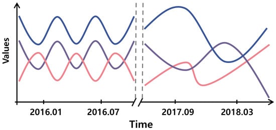
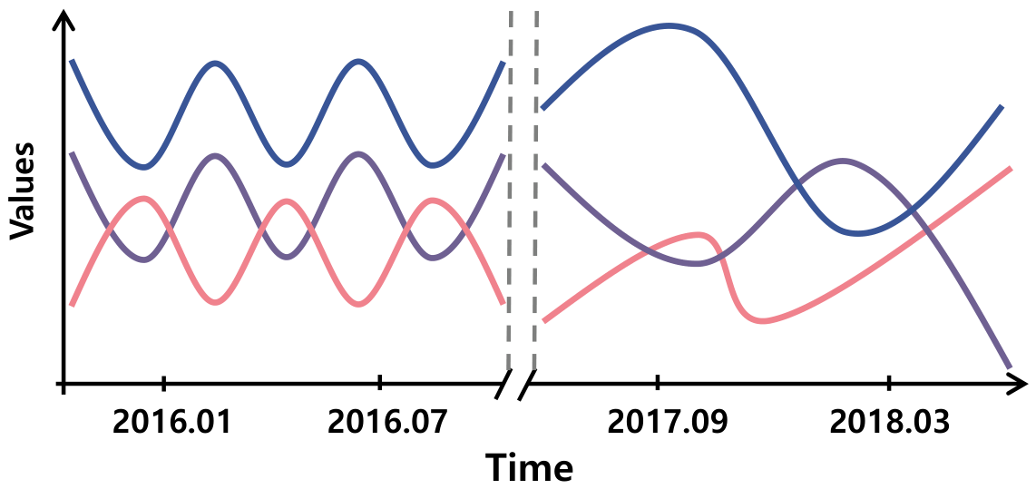
Time series forecasting plays a crucial role across numerous domains, including financial markets [1,2], transportation systems [3,4], energy management [5], and so on. With the rapid advancement of deep learning techniques in recent years, many innovative deep learning models have been proposed [6,7], demonstrating remarkable performance in this field. These models leverage complex nonlinear transformations and automated feature extraction mechanisms to effectively capture intricate temporal patterns and underlying dependencies inherent in time series data. However, real-world time series data often exhibit non-stationarity [8], wherein the statistical properties of the data evolve over time, reflecting dynamically changing patterns. Such non-stationarity presents formidable challenges for accurate forecasting. Existing models experience substantial performance deterioration when applied to data that deviates from their training distribution, a condition known as out of distribution (OOD). This performance decline primarily stems from the models’ strong reliance on the training data distribution, limiting their ability to adapt to distributional changes or domain shifts in test sets. As shown in Figure 1, the left part is regular periodic fluctuations, such as daily electricity consumption cycles driven by predictable human activity. In contrast, the sequences in the right part display different behaviors, such as sudden shifts in electricity demand caused by unexpected weather events or system anomalies, leading to noticeable shifts in the data distribution. The challenges of model generalization and resilience become particularly evident when confronted with significant distributional changes caused by unexpected events, seasonal variations, or regulatory modifications.
Figure 1.
OOD scenarios in time series.
A commonly adopted approach to addressing the OOD problem described above is to regularize the input data. These methods [8,9] often employ statistical techniques or learnable modules to normalize input subsequences, transforming them into a stable distribution. This process mitigates non-stationary effects, enabling the model to more effectively capture underlying patterns and trends within the data. After completing the prediction process, the outputs are subsequently inverse normalized to restore them to the original scale and distribution, ensuring consistency with the input data.
Although normalization techniques are effective in alleviating the OOD problem, they exhibit certain limitations in capturing evolving patterns. Specifically, the uniform scaling of input series may overlook the variations present in different time periods. Moreover, prior studies [10] have highlighted that time series data can be viewed as a composition of multiple sequences with distinct periodicities. Each periodic component reflects unique frequency characteristics, and their superposition along the time axis creates complex patterns of changes. Beneath the complex patterns of time series lie inherent features that are intrinsically tied to the core patterns of the data and remain relatively stable over time. These stable features often encapsulate the underlying structure or fundamental patterns governing the series. Their existence enables the time series to retain a degree of internal consistency despite fluctuations, forming the foundation upon which forecasting models can capture long-term trends and patterns effectively. Modeling time series solely in the time domain can lead to difficulties in disentangling frequency components and extracting these stable features embedded in the data, which affects the forecasting performance and model generalization capability.
To address the above challenges, we introduce FreqMoE, an approach that analyzes time series in the frequency domain to effectively decompose and identify distinct frequency components, enabling better capture of inherent patterns. Our method first implements a low-pass filter to eliminate high-frequency noise while preserving essential low-frequency characteristics of the time series. Subsequently, we generate multiple variant sequences by applying random masking perturbations to the original sequence. This masking strategy encourages the model to learn representations less sensitive to temporal distribution shifts by selectively obscuring temporal information, effectively simulating data incompleteness and variations. These masked variants are then processed through a Mixture of Experts (MoE) network, where each masked variant sequence is exclusively handled by a single expert in the frequency domain, and the final prediction is computed through a weighted combination of expert outputs, with weights determined by a dynamic routing mechanism. Through this architectural design, FreqMoE encourages the learning of features that are more robust to temporal distribution shifts, improving model robustness and generalization capabilities in OOD scenarios. In summary, our contributions are as follows:
- We present FreqMoE, a framework that integrates frequency-domain modeling, random masking, and Mixture of Experts routing to address OOD challenges in time series forecasting. While each component has been studied individually, their specific combination with spectrum-embedding-based dynamic routing constitutes the core contribution.
- We introduce a masking mechanism within FreqMoE to encourage robust frequency-domain representations. Meanwhile, the spectrum embedding of the input sequences enables adaptive weight assignment to the expert networks, helping the model capture stable frequency-domain patterns.
- We systematically evaluate FreqMoE on seven real-world time series datasets spanning multiple domains. Experimental results demonstrate that FreqMoE achieves competitive or leading performance compared to existing models in OOD scenarios, with the lowest performance degradation under distribution shifts.
Table 1 summarizes the positioning of FreqMoE relative to existing approaches, highlighting the integration of frequency-domain modeling, OOD robustness, and MoE architecture.
Table 1.
Positioning of FreqMoE relative to existing approaches. ✓ indicates the method possesses the corresponding capability; × indicates it does not.
2. Related Work
2.1. Frequency-Domain Analysis Methods
Recent advancements in time series forecasting have highlighted the growing significance of frequency-domain analysis methods [13,18]. FEDformer [11] integrates seasonal-trend decomposition with Fourier transformation, implementing transformer architecture in the frequency domain to capture comprehensive temporal patterns. FiLM [12] enhances long-term forecasting accuracy by combining Legendre polynomial projections for historical information representation with Fourier projections for noise reduction. Fredformer [19] leverages discrete Fourier transformation for time series decomposition and reconstruction, incorporating local frequency-independent modeling and global semantic frequency summarization to enhance prediction precision. Koopa [14] employs Fourier filtering to distinguish between time-varying and time-invariant components, implementing a hierarchical Koopman predictor module to characterize temporal dynamics. While these approaches have contributed to improvements in time series prediction, they still face challenges in adapting to distribution shifts and handling complex noise effectively.
2.2. Out-of-Distribution Analysis Methods
The out-of-distribution (OOD) phenomenon has been observed across various time series applications [20], gaining increased attention with the advancement in deep learning methodologies. Revin [9] and Stationary [8] focus on mitigating non-stationarity through normalization techniques and their inverse operations. AdaRNN [21] enhances model performance on non-stationary time series by maximizing distributional divergence across temporal intervals while maintaining consistency in hidden state distributions. Stone [22] improves generalization in spatio-temporal graph tasks by extracting invariant node representations. Diversify [15] employs an iterative approach to identify underlying invariant representations within time series data. However, these approaches predominantly rely on time-domain modeling, limiting their ability to effectively distinguish and capture characteristics of distinct frequency components within the data.
2.3. Mixture of Experts Models
The effectiveness of Mixture of Experts (MoE) architecture has been demonstrated across various domains, including time series forecasting. Time-MoE [16] implements a sparse MoE design that maintains high model capacity while reducing computational costs by selectively activating network components during prediction. Moirai-MoE [17] incorporates specialized expert networks to handle diverse temporal patterns and implements an cluster-based gating mechanism. MoLE [23] enhances existing linear-focused Long-Term Series Forecasting (LTSF) models by integrating multiple linear expert models with a routing mechanism. TimeMixer [6] proposes decomposable multiscale mixing for time series forecasting by leveraging temporal decomposition at different scales. Additionally, Pan et al. [24] propose a hybrid framework for traffic flow estimation combining Markovian models with deep learning. However, these MoE-based approaches often overlook the characteristics of different frequency components within time series data, resulting in reduced generalization capabilities when encountering OOD problems in real-world applications.
Table 2 summarizes the relative merits and limitations of the related methods.
Table 2.
Comparison of related methods: merits and limitations.
3. Preliminary Section
The Fourier transform (FT) is a fundamental mathematical tool for converting signals from the time domain to the frequency domain, enabling comprehensive analysis of signal frequency components. This transformation decomposes time series data into constituent sinusoidal waves of varying frequencies and amplitudes, thereby revealing essential characteristics including periodicity, underlying trends, and noise patterns within the sequence. Given a discrete time series , the discrete Fourier transform (DFT) is mathematically expressed as
where denotes the complex spectrum in the frequency domain, f denotes the frequency index, N is the total number of sampling points, and j is an imaginary unit satisfying . The exponential term in Equation (1) can be expanded into a combination of cosine and sine by Euler’s formula:
After substituting Equation (2) into the Fourier transform equation, can be decomposed into real and imaginary expressions:
where denotes the cosine component of the frequency f, reflecting the fundamental amplitude contribution of the signal at that frequency, and represents the sinusoidal component of the frequency f and captures the phase shift information of the signal. The complex spectrum obtained by Fourier transform not only provides information about the frequency distribution but also allows further calculation of amplitude and phase, which can be used to analyze the periodicity and amplitude characteristics of the time series:
where is the amplitude spectrum, which measures the energy distribution of the signal at different frequencies, and is the phase spectrum, which describes the phase shifts of the frequency components.
4. Methodology
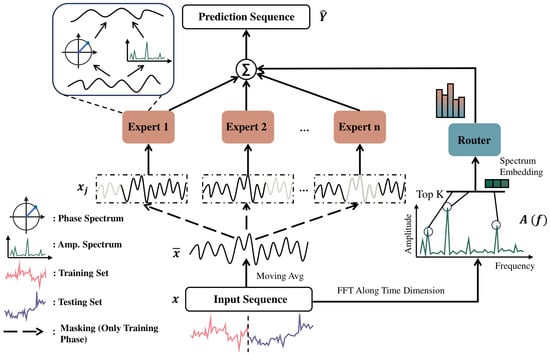
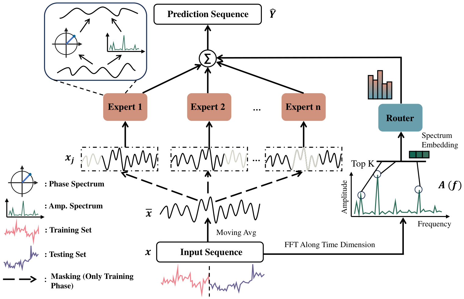
The proposed FreqMoE framework comprises three components: Temporal Smoothing Module, Masking Mechanism, and Frequency-Domain Mixture of Experts network. These integrated components work synergistically to enhance modeling and prediction capabilities for complex time series in OOD scenarios. The comprehensive architecture of FreqMoE is depicted in Figure 2.
Figure 2.
Framework of FreqMoE. The input sequence is filtered for noise via a moving average, followed by masking to encourage robust frequency-domain representations. Finally, the sequences are modeled by frequency-domain MoE to learn robust frequency-domain representations for prediction in OOD scenarios. Masking (dashed border) is applied only during training and disabled during inference. Solid arrows indicate data flow during both training and inference; dashed borders indicate operations applied only during training.
4.1. Temporal Smoothing Module
Time series collected from real-world environments are often affected by noise disturbances and unexpected events, which typically appear as outliers that deviate markedly from the overall trend. Such outliers can severely distort the model’s ability to predict future patterns, thereby undermining its robustness and generalization performance. To mitigate the influence of noise and outliers, we firstly smooth the input time sequences:
where w denotes the size of the moving window, and represents the input sequence at time t. The moving average computes the local mean within a sliding window, effectively reducing sharp local fluctuations and high-frequency noise while preserving the primary trend and low-frequency components of the series. This smoothing operation can be viewed as a low-pass filter (LPF), equivalent to applying a window filter defined as to the input sequence, where .
4.2. Masking Mechanism
After obtaining the smoothed series with H length of historical sequence and C feature variables, we introduce a masking mechanism to simulate data incompleteness. Random masking is applied independently to each channel at the point level: each time point in each channel is independently masked with probability r. This approach generates a set of masked variants, expressed as
where r represents the masking ratio, controlled within , denotes the j-th masked time series, and N is the number of masked variants produced. Random masking operations can mimic outlier gaps caused by missing sensor readings, sampling errors, or abrupt events. Incorporating these perturbations during training encourages the model to focus on underlying patterns and key features in the sequence, thereby enhancing its ability to identify stable spectral patterns and improving robustness against incomplete data.
4.3. Frequency-Domain MoE
After generating the masked variant sequences , each sequence is independently processed by an expert. To further enhance FreqMoE’s ability to capture robust frequency-domain features, we use the spectrum embedding of the input sequences to dynamically assign weights to each expert. A weighted summation of the outputs from all experts is performed to generate the final prediction results.
4.3.1. Expert Network
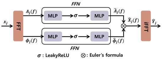
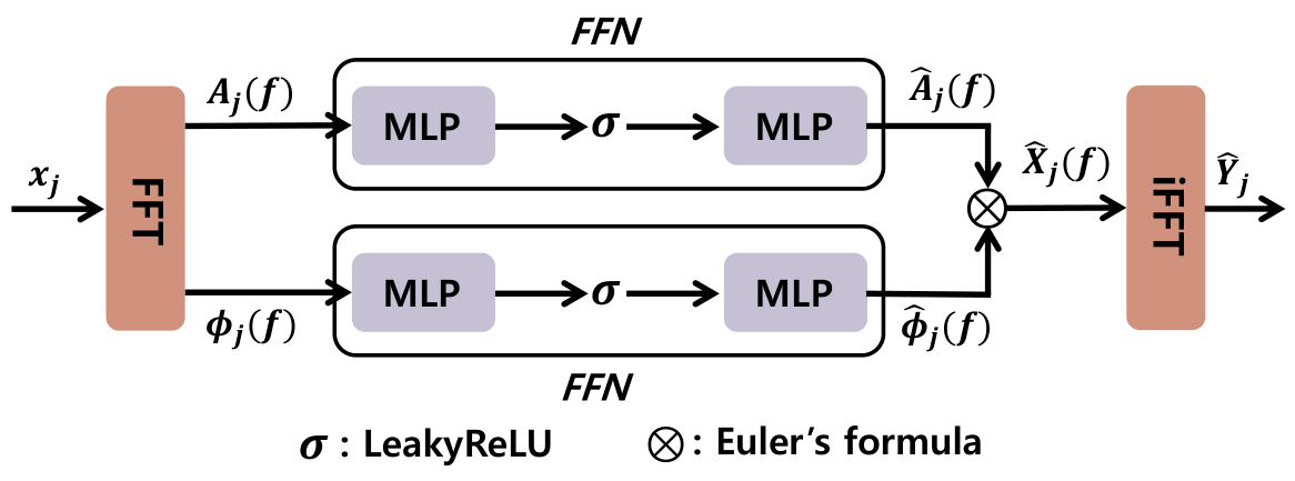
The structure of the expert network is shown in Figure 3. Given an input sequence (in the training phase, denotes the masked variant sequence, while in the testing phase, denotes the smoothed sequence and no masking operation is performed), we first transform the sequence from the time domain to the frequency domain using the FFT to obtain its frequency representation . The amplitude and phase of the sequence in the frequency domain are then calculated based on Equations (4) and (5), respectively. To enable effective feature extraction and accurate modeling of future sequences, two learnable feed-forward networks (FFNs) are introduced to independently process the amplitude and phase components:
where and denote the predicted amplitude and phase components for the future sequences, respectively. Leveraging Euler’s formula, we integrate the transformed amplitude and phase components to reconstruct the predicted representation in the frequency domain. The reconstructed frequency-domain signal is then converted back to the time domain using the inverse fast Fourier transform (iFFT), yielding the final output sequence. This process can be formulated as follows:
where denotes iFFT operation, and represent the predicted frequency-domain sequence and output sequence, respectively. We clarify the handling of different input and output lengths in the frequency domain. The input sequence of length yields a frequency representation of size after FFT. The expert FFNs map from this 49-dimensional input to a target output frequency dimension of size , where is the prediction length. The iFFT is then applied with the target length to produce the time-domain prediction. Phase wrapping is naturally handled by the arctan function in the phase computation. The process enables the model to capture meaningful patterns within the sequence from a frequency-domain perspective, facilitating the generation of accurate and robust predictions in OOD scenarios.
Figure 3.
Expert network. Independent FFNs are designed to model the amplitude and phase components of the input sequence separately.
4.3.2. Router
To enhance FreqMoE’s ability to capture robust frequency-domain features, we leverage the spectrum embedding of the input sequence to dynamically assign weights to each expert. Specifically, the input sequence x is first transformed into the frequency domain using the Fourier transform to extract its spectrum . The top k frequency components with the highest amplitudes are selected and ranked, forming the set of dominant frequency components:
where T is the length of the input sequence and denotes the amplitude of the sequence at each frequency. Using the selected frequency components, we construct the vector to serve as a spectrum embedding:
where denotes the amplitude spectrum of the input sequence at frequency . We note that the top-k amplitude selection inherently encodes frequency index information, since the selected components correspond to specific frequency positions. To maintain a consistent scale for the feature vectors, we apply the softmax function to , resulting in the normalized vector . The vector is then projected by the router weight matrix and noise weight matrix , where N is the number of experts. The routing score vector is computed as follows, where a noise term is introduced to promote balanced utilization across the experts:
where represents the learnable noise weight matrix, initialized from a positive distribution. Each element of denotes the routing score for the i-th expert. The noise term is active only during trainingto encourage exploration and balanced expert utilization, and is disabled (set to zero) during inference. The routing score of the i-th expert is processed through a softmax function to derive the corresponding routing probability . Finally, the prediction outputs from all experts are weighted and aggregated based on to produce the final prediction results of FreqMoE:
where and are learnable biases, is the prediction result of the i-th expert, N is the number of experts, and is the final prediction result. To mitigate the load balancing problem in MoE [25], an additional regularization term is incorporated into the loss function to promote balanced utilization of all experts. Specifically, we define the importance of expert i as the batch-wise sum of its routing probabilities:
where B is the batch size and is the routing probability for expert i on sample b. The auxiliary loss is then formulated as
where denotes the coefficient of variation across experts and is a scaling factor for the importance loss. The final loss function consists of two parts and can be expressed as the following equation:
where denotes the MSE loss between the prediction and the ground truth and is used to balance the expert selection process.
4.3.3. Implementation Details
We provide the following implementation details for clarity. All expert networks share the same architecture (separate FFNs for amplitude and phase) but do not share parameters—each expert has independent learnable weights. The top-k frequency component selection is fixed at for all experiments (not adaptive), selected based on the hyperparameter sensitivity analysis (Section 5.8). The relationship between the noise term and the MoE balancing loss is complementary: the noise term encourages exploration during routing in training, while the importance loss penalizes unbalanced expert utilization at the batch level.
To justify the choice of amplitude-only spectrum embedding for the router, we conduct an ablation comparing three embedding designs on the weather dataset. As shown in Table 3, amplitude-only routing achieves the best performance. Adding explicit frequency indices does not improve results, as the top-k selection already encodes frequency position information. Including phase information marginally changes the result but doubles the embedding dimension, adding complexity without a commensurate benefit. We therefore retain amplitude-only as the default.
Table 3.
Ablation of router embedding design on the weather dataset (average MSE and MAE across four horizons). Best results are highlighted in bold.
5. Experiments
5.1. Datasets
We evaluate the effectiveness of the proposed FreqMoE model using seven real-world datasets spanning multiple domains, including energy, electricity, weather, and traffic. Specifically, the datasets include ETT (ETTh1, ETTh2, ETTm1, ETTm2), weather, electricity and traffic [26,27]. To thoroughly evaluate the model’s generalization performance under OOD scenarios, we design a testing protocol. For dataset partitioning, the initial 50% of the time series data was split into training and validation sets with a 7:3 ratio. The last 25% of the data was designated as the test set. The middle 25% is intentionally excluded to create a temporal gap between the validation and test periods, increasing the likelihood of distributional divergence. This partitioning strategy not only mitigates the risk of data leakage but also introduces a temporal gap between the validation and test sets, creating a more realistic and challenging OOD scenario. We acknowledge that this temporal holdout protocol simulates naturalistic temporal drift rather than controlled synthetic distribution shifts. To rigorously quantify the distributional difference, we report Wasserstein-1 distance and Maximum Mean Discrepancy (MMD) between training and test subsequences in Table 4. The results indicate that all datasets exhibit measurable distributional shifts under this protocol. Further details are provided in Table 5.
Table 4.
Distributional distance metrics between training and test periods. W1 denotes Wasserstein-1 distance; MMD denotes Maximum Mean Discrepancy.
Table 5.
Dataset partitioning protocol for OOD evaluation.
5.2. Data Analysis
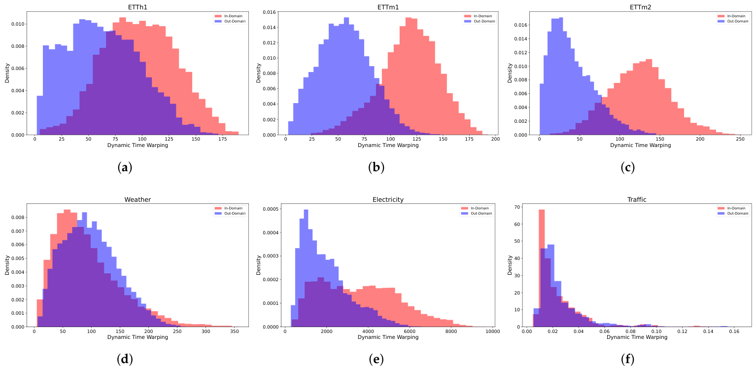
We systematically examine the differences between in-distribution and out-of-distribution scenarios by analyzing data characteristics. Specifically, we extract daily subsequences from the training and test sets and evaluate them based on statistical properties and dynamic patterns. To assess statistical properties, we compute the mean difference between the subsequences to quantify overall trend shifts. For dynamic patterns, we employ Dynamic Time Warping (DTW) [28] distance to measure variations in sequence patterns. The DTW distance is calculated using the following formula:
where x and y represent two distinct time series, while denotes the alignment path. The term refers to the local distance between the corresponding points in the two series along the alignment path.
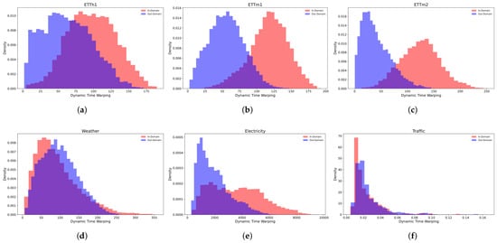
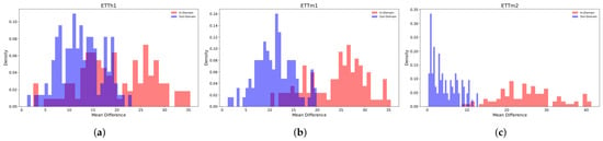
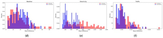
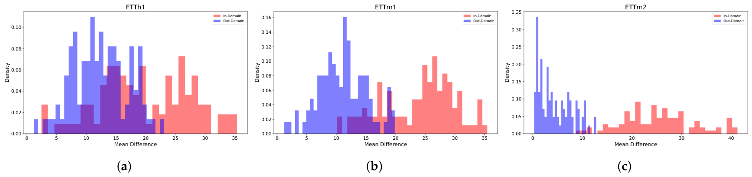
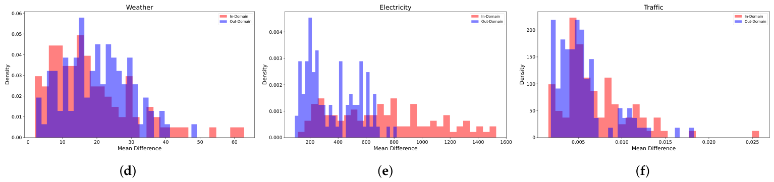
Figure 4 and Figure 5 compare the DTW distance and mean difference distributions for different datasets under in-domain and out-domain scenarios. The results reveal that the electricity-domain dataset exhibits substantial dynamic variations, with a pronounced difference between the DTW distances and mean differences between in-domain and out-domain subsequences. This indicates significant dynamic changes in this domain, potentially driven by the high sensitivity of electricity data to seasonal and demand fluctuations. In contrast, the weather- and traffic-domain datasets display smoother dynamic changes, with DTW distance and mean difference distributions for in-domain and out-domain scenarios showing closer alignment. This stability may be attributed to natural patterns or infrastructure constraints that regulate trends in weather and traffic data over time, resulting in more consistent sequence behaviors.
Figure 4.
Comparison of DTW distances across in-domain and out-domain scenarios for various datasets. “In-domain” refers to subsequences sampled from the training period; “out-domain” refers to subsequences sampled from the test (OOD) period. (a) ETTh1; (b) ETTm1; (c) ETTm2; (d) Weather; (e) Electricity; (f) Traffic.
Figure 5.
Comparison of mean differences across in-domain and out-domain scenarios for various datasets. “In-domain” refers to subsequences sampled from the training period; “out-domain” refers to subsequences sampled from the test (OOD) period. (a) ETTh1; (b) ETTm1; (c) ETTm2; (d) Weather; (e) Electricity; (f) Traffic.
5.3. Baseline and Setting
Our baseline includes several state-of-the-art time series forecasting approaches, covering both general forecasting architectures and methods specifically designed for non-stationarity and OOD scenarios:
- iTransformer [29]: A transformer-based model that embeds time series as variable tokens, employs the attention mechanism to capture multivariate correlations, and significantly improves the efficiency of computation.
- PatchTST [30]: A model that segments the time series into subsequence-level patches to serve as input tokens for the transformer and employs channel-independence techniques, significantly reducing the computational and memory overhead.
- FreTS [13]: It proposed a method using an MLP in the frequency domain by transforming a time series into the frequency domain via the DFT, applying a complex linear transformation and then returning to the time domain via inverse Fourier transform to obtain predictions.
- DLinear [31]: It outperformed the transformer-based model in the benchmark by combining trend decomposition techniques with simple linear models.
- Stationary [8]: It enhances the model’s predictive robustness in dynamic environments by smoothing the input series, standardizing its statistical properties, and mitigating the impact of distributional shifts.
- RevIN [9]: A normalization-based method specifically designed for non-stationary time series that applies reversible instance normalization to mitigate distribution shifts.
- Diversify [15]: An OOD-specific method that iteratively discovers invariant representations within time series data for improved generalization.
- TimesNet [32]: A recent frequency-domain forecasting model that transforms 1D temporal variations into 2D frequency-domain representations and applies 2D convolution.
To ensure fairness and consistency in evaluation, we adopt a fixed input length of and evaluate output lengths across all datasets for all approaches. For long-term forecasting tasks, we employ mean squared error (MSE) and mean absolute error (MAE) as evaluation metrics. All results are reported as the mean over 3 independent runs with different random seeds (42, 2024, 3407).
5.4. Model and Training Configuration
For our experiments, the masking ratio is configured to , the sliding window length of the moving average is set to 5, the number of experts is set to 4, and the frequency components are set to 4 in FreqMoE. Our model is trained with the L2 loss and the Adam optimizer [33]. The maximum number of training epochs is 10 and early stopping with a patience of 3 epochs on validation MSE is applied. Z-score normalization is applied per channel. All experiments are implemented using PyTorch 2.0.1 [34] on NVIDIA RTX A6000 48 GB GPU. The source code and configuration files for FreqMoE will be publicly released upon acceptance. More detailed modeling and training configurations are presented in Table 6.
Table 6.
Detailed description of model hyperparameters and training settings.
5.5. Main Results
The performance comparison between FreqMoE and other models is presented in Table 7. The results demonstrate that FreqMoE achieves competitive or leading performance in both MSE and MAE metrics across most prediction settings. In terms of average performance over all datasets, FreqMoE consistently ranks within the top two, further supporting its stability and effectiveness in OOD scenarios. Notably, FreqMoE achieves higher prediction accuracy with fewer parameters compared to mainstream transformer-based models, achieving better average performance than iTransformer across most evaluated datasets. On ETT datasets, DLinear remains competitive in some settings, while FreqMoE shows particularly strong results on the weather, electricity, and traffic datasets. The performance of FreqMoE can be attributed to its frequency-domain analysis combined with the masking and MoE routing mechanism, enabling the model to capture robust frequency-domain patterns from historical sequences. Additionally, the integration of a dynamic routing mechanism allows the model to adapt flexibly to varying data distributions, improving predictive accuracy and robustness against out-of-distribution data.
Table 7.
Full results of multivariate time series forecasting with prediction length . Lower MSE and MAE represent better performance. The best results are bolded and the second best results are underlined.
Statistical Significance. To assess the statistical significance of FreqMoE’s performance advantages, we conducted one-sided paired t-tests using the following protocol. The metric is MSE averaged across the four prediction horizons () per dataset. Each horizon-level MSE value, computed over the full test set and averaged over 3 independent random seeds (42, 2024, 3407), serves as a paired observation. FreqMoE is compared against each baseline across the seven datasets. The win/tie/loss summary at is presented in Table 8.
Table 8.
Statistical significance summary: number of datasets (out of 7) where FreqMoE significantly outperforms each baseline (one-sided paired t-test, ).
FreqMoE achieves significantly lower MSE () than iTransformer, FreTS, Stationary, and Diversify on all seven datasets and significantly outperforms PatchTST, RevIN, and TimesNet on the majority of datasets. On ETTm1, DLinear remains competitive, consistent with the per-dataset results in Table 7.
5.6. Ablation Experiments
Table 9 presents the results of ablation experiments conducted on the components of FreqMoE. It can be observed that the complete FreqMoE model achieves the best performance. Removing any component leads to a decrease in performance, with the removal of the frequency-domain MoE causing the most significant impact. Specifically, the MAE increases by 5.5% on weather and 6.2% on electricity, highlighting the critical role of the frequency-domain MoE. The removal of the Masking Mechanism also results in performance degradation, underscoring the importance of this regularization strategy in enhancing the model’s robustness. Additionally, the Temporal Smoothing Module filters out noise caused by unexpected events, enhancing FreqMoE’s capability to capture the intrinsic characteristics of the sequence.
Table 9.
Ablation experiments of FreqMoE. w/o Mask, w/o MA, and w/o MoE represent the removal of Masking Mechanism, Temporal Smoothing Module, and frequency-domain MoE, respectively. Random Routing replaces spectrum-based routing with uniform weights. Time-domain MoE applies the MoE in the time domain instead of the frequency domain. The best results are bolded.
We further include three additional ablation variants. Random Routing replaces the spectrum-embedding-based routing with uniform weights, resulting in noticeable performance degradation, which demonstrates the benefit of spectrum-based expert selection. Time-domain MoE applies the MoE architecture in the time domain instead of the frequency domain, showing larger degradation that demonstrates the importance of frequency-domain modeling. w/o Mask + w/o MA removes both the masking and moving average components simultaneously, resulting in the largest degradation, indicating that these components provide complementary benefits.
5.7. Analysis of Model Degradation
Table 10 evaluates the performance of various models across both in-distribution and out-of-distribution scenarios, along with the corresponding performance decay. For the degradation analysis, both in-distribution (IN) and out-of-distribution (OOD) results for all models were obtained under our unified experimental framework. The IN results use a standard chronological split (first 70% for training, next 20% for validation, last 10% for testing, following the protocol from [29]), while the OOD results use our temporal-gap protocol (Table 5). All models were run with the same implementation framework, optimization settings, and random seeds to ensure fair comparison. In the in-distribution prediction tasks, all models demonstrate relatively stable performance. However, under out-of-distribution scenarios, the baseline models experience significant performance degradation. On the large-scale traffic dataset, the MSE of iTransformer increases from 0.428 to 0.813, reflecting a decay of 89.9%. In contrast, performance decay of our proposed FreqMoE is only 28.2%, which is lower than that of the other models. Notably, the OOD-specific baselines RevIN, Diversify, and TimesNet also show significant degradation on traffic (59.6–66.0%), while FreqMoE achieves the lowest average degradation across the evaluated datasets, though the advantage is not uniform across all datasets and horizons. For example, on ETTh2, FreqMoE still exhibits substantial absolute degradation (OOD MSE of 1.156, a 206.6% increase over the IN setting), and on ETTh1, FreTS achieves a comparable degradation rate (98.9% vs. FreqMoE’s 98.0%). The primary advantage of FreqMoE is most pronounced on electricity (17.3%) and traffic (28.2%), where it substantially outperforms all baselines. These experimental results demonstrate the effectiveness of FreqMoE in addressing OOD challenges on average, though we note that the robustness advantage is dataset dependent rather than universal.
Table 10.
Average MSE for in-distribution (IN) and out-of-distribution (OOD) scenarios with percentage decrease (Dec. %). The best results are bolded and the second best results are underlined.
5.8. Hyperparameter Sensitivity
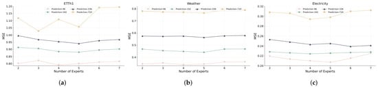
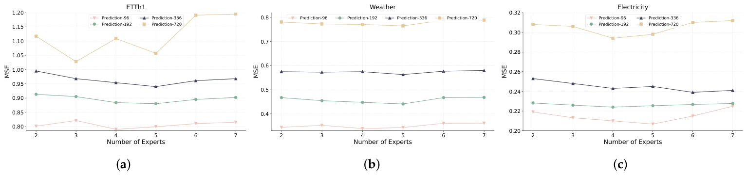
To analyze the sensitivity of FreqMoE to key parameters, we conducted a systematic study of the number of experts, masking ratio, moving average window size, and top-k frequency components. As illustrated in Figure 6, the model’s prediction performance demonstrates a distinct nonlinear relationship with the number of experts. Specifically, when the number of experts is small, increasing their count significantly reduces prediction error. However, once the number of experts surpasses a certain threshold, the model’s performance plateaus and eventually declines, suggesting that while additional experts increase the model’s capacity, they also elevate the risk of overfitting.
Figure 6.
Impact of the number of experts on prediction performance across different datasets. (a) ETTh1; (b) Weather; (c) Electricity.
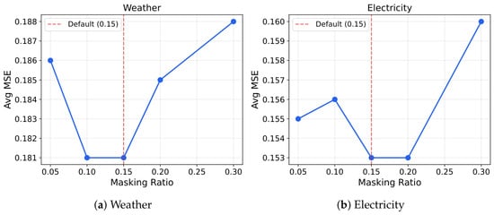
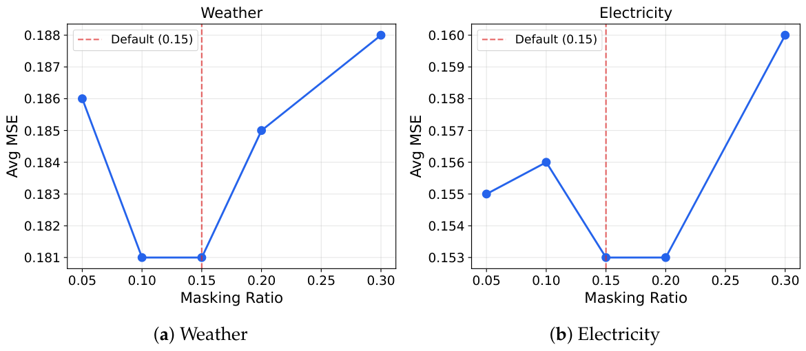
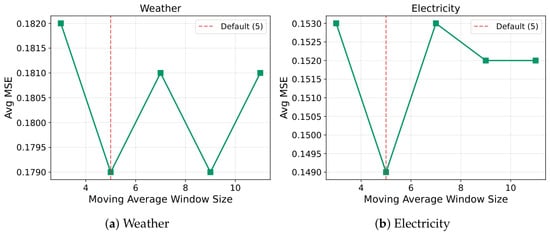
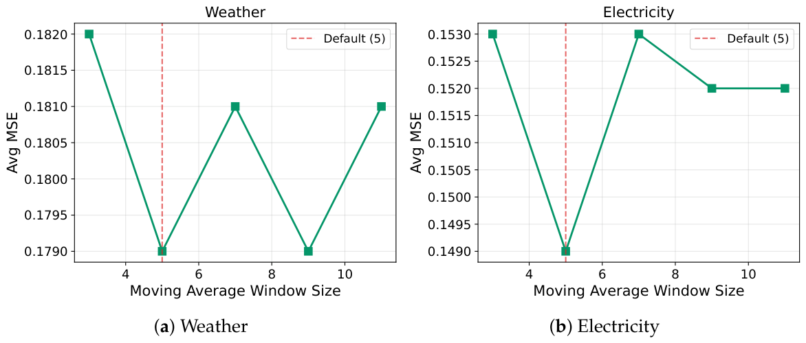
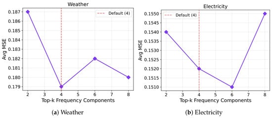
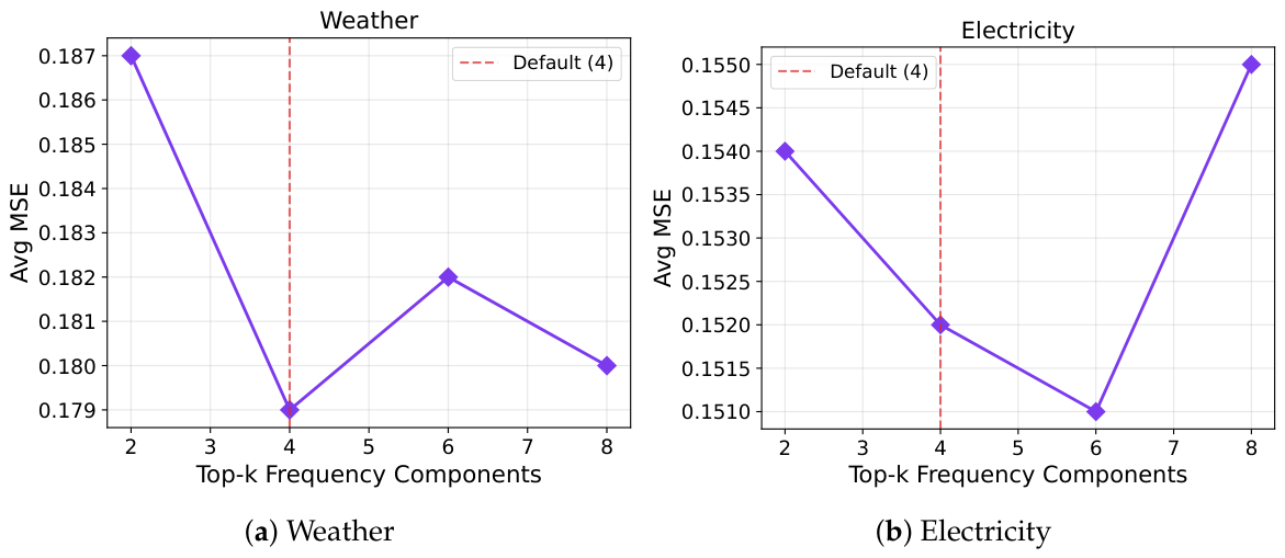
Figure 7 presents the sensitivity analysis for the masking ratio. The results show that provides a good balance: too small a ratio provides insufficient regularization, while too large a ratio removes excessive information. Figure 8 shows the sensitivity to the moving average window size, with yielding the best overall performance. Figure 9 presents the sensitivity to the top-k frequency components, indicating that provides a good trade-off between information retention and routing dimensionality.
Figure 7.
Impact of the masking ratio on prediction performance. The red dashed line indicates the default value ().
Figure 8.
Impact of the moving average window size on prediction performance. The red dashed line indicates the default value ().
Figure 9.
Impact of the top-k frequency components on prediction performance. The red dashed line indicates the default value ().
5.9. Efficiency Analysis
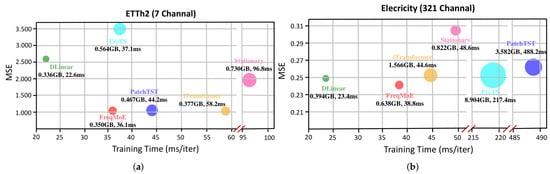
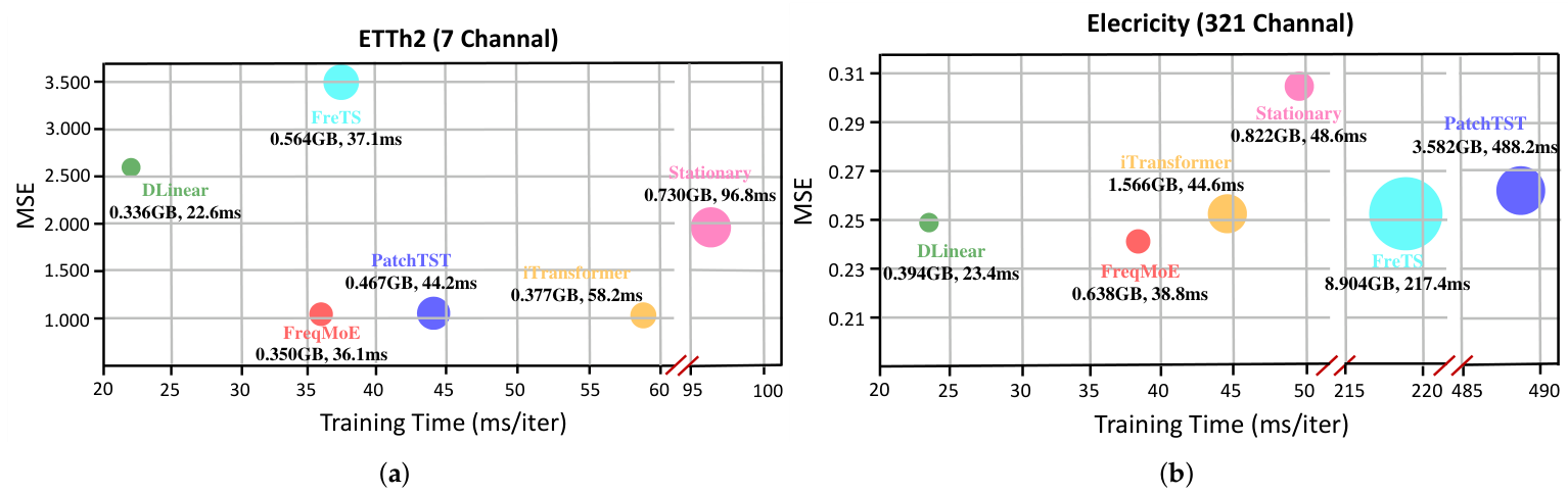
We comprehensively evaluate the performance of models in terms of predictive accuracy, parameter count, computational cost, inference latency, memory usage, and training speed. As illustrated in Figure 10 and Table 11, FreqMoE achieves a favorable balance between computational efficiency and prediction accuracy. All models are evaluated under identical conditions—input length: 96, prediction length: 96, batch size: 32, full precision (FP32)—on a single NVIDIA RTX A6000 48GB GPU, with all baselines implemented under the same PyTorch framework with consistent optimization settings. Specifically, FreqMoE has only 0.42M parameters, reducing GPU memory usage by 59.6% and shortening training time by 13.1% relative to the benchmark iTransformer. Moreover, compared to FreTS, an established frequency-domain temporal modeling framework, FreqMoE achieves superior predictive capabilities while demanding merely 7.16% of the GPU memory resources and 17.84% of the training time.
Figure 10.
Model efficiency comparison on the ETTh2 and electricity datasets. (a) ETTh2; (b) Electricity.
Table 11.
Comprehensive efficiency comparison across models. Params, FLOPs, and inference latency are reported. The best results are bolded.
5.10. Interpretability Analysis
To provide interpretability beyond prediction error metrics, we analyze the learned representations and routing behavior of FreqMoE.
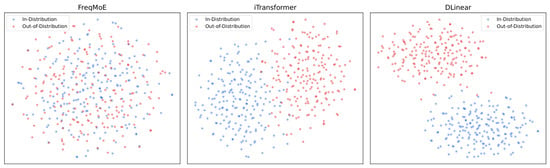
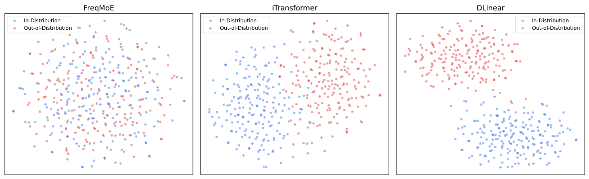
Representation Visualization. Figure 11 shows t-SNE visualizations of frequency-domain embeddings from FreqMoE, iTransformer, and DLinear, comparing in-distribution and OOD segments. FreqMoE produces more overlapping embeddings across distributions, providing qualitative evidence consistent with more aligned representations across distributions. We note that t-SNE visualizations are suggestive rather than conclusive; the observed overlap is consistent with reduced distributional sensitivity but does not constitute formal proof of invariant representation learning.
Figure 11.
t-SNE visualization of learned embeddings from FreqMoE, iTransformer, and DLinear. Blue points represent in-distribution segments; red points represent OOD segments. FreqMoE produces more aligned representations across distributions.
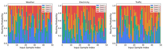
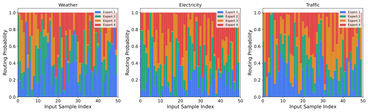
Routing Probability Visualization. Figure 12 visualizes the expert routing probability distribution across representative inputs from different datasets. The results show that experts exhibit distinct activation patterns correlated with input frequency characteristics, indicating suggestive evidence of meaningful frequency-domain specialization.
Figure 12.
Expert routing probability distribution across weather, electricity, and traffic datasets. Each color represents the routing probability assigned to a specific expert.
6. Conclusions and Future Work
In this paper, we propose FreqMoE, a framework that integrates frequency-domain modeling, random masking, and Mixture of Experts routing for time series forecasting in OOD scenarios. Our main contributions are: (1) a frequency-domain MoE architecture where each expert independently models amplitude and phase components of the spectrum; (2) a spectrum-embedding-based router that dynamically assigns expert weights based on input frequency characteristics; (3) a masking-based regularization strategy that encourages robust frequency-domain representations. Experimental results on seven real-world datasets demonstrate that FreqMoE achieves competitive or leading performance compared to existing models in OOD scenarios, with the lowest performance degradation under temporal distribution shifts.
Limitations and Future Work. This study has several limitations. First, our OOD evaluation relies on temporal holdout, which represents naturalistic but not controlled distribution shifts; future work should evaluate them under synthetic shift scenarios and on datasets with documented domain shifts. Second, we do not provide formal theoretical guarantees for invariant feature learning; such analysis through invariant risk minimization frameworks would strengthen the theoretical foundation. Third, the evaluation is limited to benchmark datasets; real-world deployment scenarios would provide stronger validation. Fourth, the masking strategy simulates point-level data incompleteness but may not fully capture complex shift types such as seasonal regime changes or structural breaks. Future work will explore adaptive masking strategies, extend to multivariate frequency routing, and investigate theoretical connections to invariant risk minimization.
Author Contributions
Conceptualization, A.S. and Z.L.; methodology, A.S.; validation, A.S. and Z.L.; formal analysis, T.W.; investigation, Z.L. and T.W.; data curation, Z.L. and T.W.; writing—original draft preparation, Z.L.; writing—review and editing, A.S. and Z.L.; visualization, T.W.; supervision, A.S.; project administration, A.S. All authors have read and agreed to the published version of the manuscript.
Funding
This research received no external funding.
Institutional Review Board Statement
Not applicable.
Informed Consent Statement
Not applicable.
Data Availability Statement
The ETT dataset can be acquired at https://github.com/zhouhaoyi/ETDataset (accessed on 9 May 2026), the Weather dataset can be acquired at https://www.bgc-jena.mpg.de/wetter/ (accessed on 9 May 2026), the Electricity dataset can be acquired at https://archive.ics.uci.edu/dataset/321/electricityloaddiagrams/ (accessed on 9 May 2026), and the Traffic dataset can be acquired at https://pems.dot.ca.gov/ (accessed on 9 May 2026). The source code, configuration files, and experiment scripts for FreqMoE are being organized and will be released as a public GitHub repository.
Conflicts of Interest
The authors declare no conflicts of interest.
References
- Li, Z.; Han, J.; Song, Y. On the forecasting of high-frequency financial time series based on ARIMA model improved by deep learning. J. Forecast. 2020, 39, 1081–1097. [Google Scholar]
- Yang, M.; Wang, J. Adaptability of financial time series prediction based on BiLSTM. Procedia Comput. Sci. 2022, 199, 18–25. [Google Scholar] [CrossRef] [Scilit]
- Ma, C.; Dai, G.; Zhou, J. Short-term traffic flow prediction for urban road sections based on time series analysis and LSTM_BILSTM method. IEEE Trans. Intell. Transp. Syst. 2021, 23, 5615–5624. [Google Scholar] [CrossRef] [Scilit]
- Zhang, J.; Chen, F.; Cui, Z.; Guo, Y.; Zhu, Y. Deep learning architecture for short-term passenger flow forecasting in urban rail transit. IEEE Trans. Intell. Transp. Syst. 2020, 22, 7004–7014. [Google Scholar] [CrossRef] [Scilit]
- Deb, C.; Zhang, F.; Yang, J.; Lee, S.E.; Shah, K.W. A review on time series forecasting techniques for building energy consumption. Renew. Sustain. Energy Rev. 2017, 74, 902–924. [Google Scholar] [CrossRef] [Scilit]
- Wang, S.; Wu, H.; Shi, X.; Hu, T.; Luo, H.; Ma, L.; Zhang, J.Y.; Zhou, J. TimeMixer: Decomposable Multiscale Mixing for Time Series Forecasting. In Proceedings of the Twelfth International Conference on Learning Representations, Vienna, Austria, 7–11 May 2024. [Google Scholar]
- Wu, H.; Xu, J.; Wang, J.; Long, M. Autoformer: Decomposition transformers with auto-correlation for long-term series forecasting. Adv. Neural Inf. Process. Syst. 2021, 34, 22419–22430. [Google Scholar] [CrossRef] [Scilit]
- Liu, Y.; Wu, H.; Wang, J.; Long, M. Non-stationary transformers: Exploring the stationarity in time series forecasting. Adv. Neural Inf. Process. Syst. 2022, 35, 9881–9893. [Google Scholar] [CrossRef] [Scilit]
- Kim, T.; Kim, J.; Tae, Y.; Park, C.; Choi, J.H.; Choo, J. Reversible instance normalization for accurate time-series forecasting against distribution shift. In Proceedings of the Tenth International Conference on Learning Representations, Virtual, 25–29 April 2022. [Google Scholar]
- Proakis, J.G.; Manolakis, D.G. Digital Signal Processing: Principles Algorithms and Applications; Pearson India Education: Tamil Nadu, India, 2007. [Google Scholar]
- Zhou, T.; Ma, Z.; Wen, Q.; Wang, X.; Sun, L.; Jin, R. Fedformer: Frequency enhanced decomposed transformer for long-term series forecasting. In Proceedings of the 39th International Conference on Machine Learning; PMLR: Baltimore, MD, USA, 2022; pp. 27268–27286. [Google Scholar] [CrossRef] [Scilit]
- Zhou, T.; Ma, Z.; Wen, Q.; Sun, L.; Yao, T.; Yin, W.; Jin, R. Film: Frequency improved legendre memory model for long-term time series forecasting. Adv. Neural Inf. Process. Syst. 2022, 35, 12677–12690. [Google Scholar] [CrossRef] [Scilit]
- Yi, K.; Zhang, Q.; Fan, W.; Wang, S.; Wang, P.; He, H.; An, N.; Lian, D.; Cao, L.; Niu, Z. Frequency-domain MLPs are more effective learners in time series forecasting. Adv. Neural Inf. Process. Syst. 2024, 36, 76656–76679. [Google Scholar] [CrossRef] [Scilit]
- Liu, Y.; Li, C.; Wang, J.; Long, M. Koopa: Learning non-stationary time series dynamics with koopman predictors. Adv. Neural Inf. Process. Syst. 2023, 36, 12271–12290. [Google Scholar] [CrossRef] [Scilit]
- Lu, W.; Wang, J.; Sun, X.; Chen, Y.; Ji, X.; Yang, Q.; Xie, X. Diversify: A general framework for time series out-of-distribution detection and generalization. IEEE Trans. Pattern Anal. Mach. Intell. 2024, 46, 4534–4550. [Google Scholar] [CrossRef] [Scilit]
- Shi, X.; Wang, S.; Nie, Y.; Li, D.; Ye, Z.; Wen, Q.; Jin, M. Time-MoE: Billion-Scale Time Series Foundation Models with Mixture of Experts. arXiv 2024, arXiv:2409.16040. [Google Scholar]
- Liu, X.; Liu, J.; Woo, G.; Aksu, T.; Liang, Y.; Zimmermann, R.; Liu, C.; Li, J.; Savarese, S.; Xiong, C.; et al. Moirai-MoE: Empowering Time Series Foundation Models with Sparse Mixture of Experts. arXiv 2025, arXiv:2410.10469. [Google Scholar]
- Yi, K.; Fei, J.; Zhang, Q.; He, H.; Hao, S.; Lian, D.; Fan, W. FilterNet: Harnessing frequency filters for time series forecasting. arXiv 2024, arXiv:2411.01623. [Google Scholar]
- Piao, X.; Chen, Z.; Murayama, T.; Matsubara, Y.; Sakurai, Y. Fredformer: Frequency Debiased Transformer for Time Series Forecasting. arXiv 2024, arXiv:2406.09009. [Google Scholar]
- Wang, H.; Chen, J.; Pan, T.; Dong, Z.; Jiang, R.; Song, X. Evaluating the Generalization Ability of Spatiotemporal Model in Urban Scenario. IEEE Trans. Mob. Comput. 2025, 24, 13535–13548. [Google Scholar] [CrossRef] [Scilit]
- Du, Y.; Wang, J.; Feng, W.; Pan, S.; Qin, T.; Xu, R.; Wang, C. Adarnn: Adaptive learning and forecasting of time series. In Proceedings of the 30th ACM International Conference on Information & Knowledge Management, Queensland, Australia, 1–5 November 2021; pp. 402–411. [Google Scholar]
- Wang, B.; Ma, J.; Wang, P.; Wang, X.; Zhang, Y.; Zhou, Z.; Wang, Y. Stone: A spatio-temporal ood learning framework kills both spatial and temporal shifts. In Proceedings of the 30th ACM SIGKDD Conference on Knowledge Discovery and Data Mining, Barcelona, Spain, 25–29 August 2024; pp. 2948–2959. [Google Scholar]
- Ni, R.; Lin, Z.; Wang, S.; Fanti, G. Mixture-of-Linear-Experts for Long-term Time Series Forecasting. In Proceedings of the 27th International Conference on Artificial Intelligence and Statistics; PMLR: Valencia, Spain, 2024; pp. 4672–4680. [Google Scholar]
- Pan, Y.A.; Guo, J.; Chen, Y.; Cheng, Q.; Li, W.; Liu, Y. A fundamental diagram based hybrid framework for traffic flow estimation and prediction by combining a Markovian model with deep learning. Expert Syst. Appl. 2024, 238, 122219. [Google Scholar] [CrossRef] [Scilit]
- Shazeer, N.; Mirhoseini, A.; Maziarz, K.; Davis, A.; Le, Q.; Hinton, G.; Dean, J. Outrageously Large Neural Networks: The Sparsely-Gated Mixture-of-Experts Layer. arXiv 2017, arXiv:1701.06538. [Google Scholar]
- Zhou, H.; Zhang, S.; Peng, J.; Zhang, S.; Li, J.; Xiong, H.; Zhang, W. Informer: Beyond efficient transformer for long sequence time-series forecasting. In Proceedings of the AAAI Conference on Artificial Intelligence, Virtual, 19–21 May 2021; Volume 35, pp. 11106–11115. [Google Scholar]
- Lai, G.; Chang, W.C.; Yang, Y.; Liu, H. Modeling Long- and Short-Term Temporal Patterns with Deep Neural Networks. In Proceedings of the 41st International ACM SIGIR Conference on Research & Development in Information Retrieval, New York, NY, USA, 8–12 July 2018; SIGIR ’18. pp. 95–104. [Google Scholar] [CrossRef] [Scilit]
- Müller, M. Dynamic time warping. In Information Retrieval for Music and Motion; Springer: Berlin/Heidelberg, Germany, 2007; pp. 69–84. [Google Scholar]
- Liu, Y.; Hu, T.; Zhang, H.; Wu, H.; Wang, S.; Ma, L.; Long, M. itransformer: Inverted transformers are effective for time series forecasting. arXiv 2024, arXiv:2310.06625. [Google Scholar]
- Nie, Y.; Nguyen, N.H.; Sinthong, P.; Kalagnanam, J. A Time Series is Worth 64 Words: Long-term Forecasting with Transformers. arXiv 2022, arXiv:2211.14730. [Google Scholar]
- Zeng, A.; Chen, M.; Zhang, L.; Xu, Q. Are transformers effective for time series forecasting? In Proceedings of the AAAI Conference on Artificial Intelligence, Washington, DC, USA, 7–14 February 2023; Volume 37, pp. 11121–11128. [Google Scholar]
- Wu, H.; Hu, T.; Liu, Y.; Zhou, H.; Wang, J.; Long, M. Timesnet: Temporal 2d-variation modeling for general time series analysis. In Proceedings of the Eleventh International Conference on Learning Representations, Kigali, Rwanda, 1–5 May 2023. [Google Scholar]
- Kingma, D.P.; Ba, J. Adam: A method for stochastic optimization. arXiv 2014, arXiv:1412.6980. [Google Scholar]
- Paszke, A.; Gross, S.; Massa, F.; Lerer, A.; Bradbury, J.; Chanan, G.; Killeen, T.; Lin, Z.; Gimelshein, N.; Antiga, L.; et al. Pytorch: An imperative style, high-performance deep learning library. Adv. Neural Inf. Process. Syst. 2019, 32, 8026–8037. [Google Scholar] [CrossRef] [Scilit]

Disclaimer/Publisher’s Note: The statements, opinions and data contained in all publications are solely those of the individual author(s) and contributor(s) and not of MDPI and/or the editor(s). MDPI and/or the editor(s) disclaim responsibility for any injury to people or property resulting from any ideas, methods, instructions or products referred to in the content. |
© 2026 by the authors. Licensee MDPI, Basel, Switzerland. This article is an open access article distributed under the terms and conditions of the Creative Commons Attribution (CC BY) license.