


Abstract
Image-based measurement of chopped maize stalk length remains difficult because the fragments are often slender, curved, touching, or partly overlapped. Bounding-box dimensions are therefore not reliable for length estimation, and manual measurement is too slow for repeated quality assessment. In this study, we developed a YOLO11n-based visual framework for measuring chopped maize stalk length under fixed imaging conditions. The dataset contained 1127 images collected on a laboratory platform and covered stalk lengths of 10–150 mm, different moisture states, and isolated, touching, and overlapping arrangements. To obtain more stable regions of interest, the YOLO11n detector was modified with large separable kernel attention (LSKA), a lightweight cross-scale decoupled detection (LSCD) head, and Wise intersection over union version 3 (WIoU v3). The detected stalk regions were then processed by local segmentation, morphological refinement, skeleton extraction, longest-path calculation, and washer-based scale conversion. The modified detector reached 94.8% precision, 90.4% recall, 96.5% mAP@0.5, and 71.1% mAP@0.5:0.95, with a detector inference speed of 174 FPS. In the length-measurement test, the mean relative errors were 5.8%, 8.3%, and 10.4% for the <40 mm, 40–80 mm, and >80 mm groups, respectively. Across all evaluated fragments, the complete pipeline produced an MAE of 6.0 mm, an RMSE of 9.4 mm, and a mean relative error of 8.2%. The framework therefore provides a practical way to measure chopped maize stalk length under controlled imaging conditions, although long, curved, and cluttered fragments still caused most of the remaining errors.
1. Introduction
Maize is a major crop for both food production and biomass utilization [1,2]. Beyond grain production, maize stalks provide an important residue resource for silage, fodder, bioenergy, and related applications [3,4]. The length of chopped stalks directly affects residue handling and material quality. Fragments that are too long or highly uneven are more difficult to compact, transport, store, and process. In silage and fodder production, long fragments may reduce packing density and fermentation uniformity, whereas overly short fragments can increase chopping energy consumption and damage the physical structure of the material [5]. Chopped length and length uniformity are also useful indicators of machine performance because they reflect chopping quality, blade condition, and the suitability of operating parameters [6,7]. Accurate and efficient measurement of chopped maize stalk length is therefore important for residue management, biomass estimation, fodder quality control, and harvesting-machine evaluation.
Image-based methods have been widely explored for measuring particle size and plant morphology. Igathinathane et al. used digital images to measure particle shape and size distribution, demonstrating the potential of image processing to reduce manual measurement [8]. Nigon et al. developed a system for assessing crop-residue particle-size distribution, a parameter closely related to residue handling and machine performance [9]. In maize phenotyping, Wu et al. extracted plant skeletons from 3D point clouds to estimate structural traits, and Miao et al. used skeleton-guided stem-leaf separation to measure plant height, stem height, and leaf length [10,11]. More recently, Zhao et al. proposed LenRuler, an automated radicle-length measurement method that combines SAM-based segmentation, skeleton extraction, and geodesic-distance calculation for rice seeds and multicrop validation [12]. These studies show that image-based and skeleton-based approaches can be effective for elongated biological materials. Chopped maize stalk fragments, however, present a more difficult measurement target because they are shorter, narrower, more irregular, and more likely to touch or overlap. These characteristics limit the reliability of direct particle-size analysis and box-based measurement.
Manual sampling, laser-based measurement, and photoelectric sensing can provide reference values, but they are less suitable for continuous, high-throughput residue monitoring [13]. Machine vision offers greater flexibility and can be adapted to different imaging scenes. Early vision-based methods mainly relied on thresholding, edge detection, color segmentation, and morphological operations to separate plant residues from the background [14,15]. Such methods work well when imaging conditions are stable and the target has clear contrast with the background. In practice, chopped stalk fragments vary in color, bend in different directions, touch or overlap with each other, and are often mixed with loose fibers and debris. Under these conditions, extracted contours can become incomplete, broken, or connected to neighboring fragments [16]. Data augmentation can improve robustness in vision tasks with limited samples, but its effect still depends on the task and dataset characteristics [17].
Deep learning detectors have improved target localization in complex vision tasks and are now widely used in real-time monitoring [18,19,20]. Most YOLO-based detectors, however, are designed to locate objects rather than to measure their physical length directly [21]. This distinction is important for chopped maize stalks. Because the fragments are slender, curved, broken, or partly overlapped, neither the long side nor the diagonal of a bounding box can represent the actual centerline length. Even a small box shift or truncation can affect the subsequent length calculation. Shadows, overlapping fragments, and loose fibers may further weaken boundary continuity [22,23]. For this reason, detection is better used as a localization step that provides regions of interest, rather than as a direct length-measurement method.
To address these problems, we developed a YOLO11n-based visual framework for measuring chopped maize stalk length. The key idea is to use detection for localization only, rather than treating the detected box as the measurement result. The model first locates stalk fragments and the calibration washer. Each detected stalk region is then processed by ROI segmentation, skeleton extraction, longest-path analysis, and washer-based scale conversion to obtain the physical length. In this way, the method avoids relying on the long side or diagonal of a bounding box, which cannot represent the true path length of slender, curved, touching, or partially overlapped stalk fragments.
The main contributions of this study are as follows:
- A detection-guided measurement framework was developed for chopped maize stalks. The framework separates target localization from length measurement. The detector provides local ROIs, and the stalk length is measured from the skeleton path within each ROI. This design is better suited to irregular stalk fragments than direct box-based measurement.
- YOLO11n was modified to provide more stable ROIs for the subsequent measurement steps. LSKA was used to enhance the spatial continuity of slender and curved stalk bodies. An LSCD head was introduced to improve localization consistency across target scales, and WIoU v3 was adopted to stabilize bounding-box regression. These changes address three practical difficulties in chopped stalk detection: weak continuity of slender targets, unstable scale response, and localization errors that can be carried into the measurement stage.
- A complete skeleton-based length measurement procedure was constructed and evaluated. After ROI extraction, local segmentation, morphological refinement, skeleton extraction, branch pruning, and longest-path analysis were used to obtain the pixel length of each stalk fragment. The pixel length was then converted to physical length using the washer-based scale coefficient. The framework was evaluated through model comparison, ablation experiments, additional AP metrics, and length-measurement errors to examine how ROI localization affects final measurement accuracy.
2. Materials and Methods
2.1. Imaging Setup and Dataset
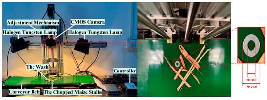
Figure 1 shows the laboratory imaging setup for chopped maize stalk samples. The system included a top-view RGB CMOS camera (LT 1080P, USB 2.0), two halogen tungsten lamps, a conveyor belt, and a control unit. Chopped maize stalks and a calibration washer were placed in the same field of view for image acquisition, scale conversion, and length measurement.
Figure 1.
Laboratory image acquisition system for chopped maize stalk samples.
The camera was fixed vertically above the conveyor belt at a working distance of 230 mm. Images were resized to 640 × 640 pixels before model training and inference, giving an approximate image scale of 10 px/mm. Two halogen tungsten lamps were positioned symmetrically on both sides of the imaging area at an incidence angle of about 45°. A dark green PVC conveyor belt served as the background to increase contrast with the chopped stalks.
A stainless-steel washer was included in each image as the calibration reference. As shown in Figure 1, the washer had an inner diameter of 10.0 mm and an outer diameter of 21.8 mm, and the inner diameter was used for scale calibration. Let d0 (mm) be the true inner diameter of the washer, where d0 = 10.0 mm, and let dp (px) be the corresponding inner diameter in pixels. Definition of the main variables and symbols see Table A1. The scale coefficient ks was calculated as
where ks is expressed in mm/px. After the pixel length of a stalk fragment was obtained, its physical length was calculated as
where lp is the pixel length and lm is the converted physical length.
A total of 1127 images were collected over 10 days. The dataset covered stalk lengths from 10 to 150 mm and included moisture states ranging from fresh green stalks to dry yellow residues. To reflect common material distributions during operation, samples were arranged as isolated fragments, touching fragments, and overlapping piles. The calibration washer was kept in every image.
All images were manually annotated using LabelImg (v1.8.6). Two classes were defined: chopped maize stalk and calibration washer. For stalk annotation, the bounding box was drawn around the dense main body rather than loose terminal fibers to reduce label noise and maintain consistency with the later length-measurement procedure. Fragments at the image boundary were excluded when their main bodies were severely incomplete. Small debris and scattered fiber clusters were treated as background. Annotation examples are shown in Figure 2.
Figure 2.
Examples of annotated images under different sample conditions: (a) isolated arrangement; (b) touching arrangement; (c) overlapping pile-up with fiber interference; (d) slender and curved targets; (e) mixed long and short fragments; (f) dry stalk sample.
The dataset was randomly divided into training, validation, and test sets at an 8:1:1 ratio, corresponding to 903, 112, and 112 images, respectively. In total, 7421 stalk boxes and 1127 washer boxes were annotated, with an average of 6.58 stalk instances per image. The mean long side, short side, and aspect ratio of the stalk boxes were 209.57 px, 28.06 px, and 8.17, respectively. The high aspect ratio and variable target scale made stable localization and length measurement more difficult.
2.2. YOLO11n-Based Detection Framework
2.2.1. Baseline YOLO11n Model
In the proposed length-measurement pipeline, the detector serves as the front end. It does not estimate stalk length directly, but locates stalk fragments and provides regions of interest (ROIs) for the subsequent segmentation and skeleton-extraction steps. The detector therefore needs stable localization, sufficient speed, and a lightweight structure for possible online use. YOLO11n was selected as the baseline because it provides a compact architecture with a favorable balance between detection accuracy and inference speed.
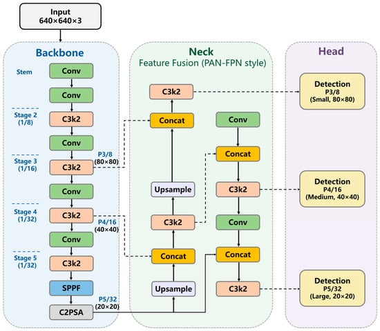
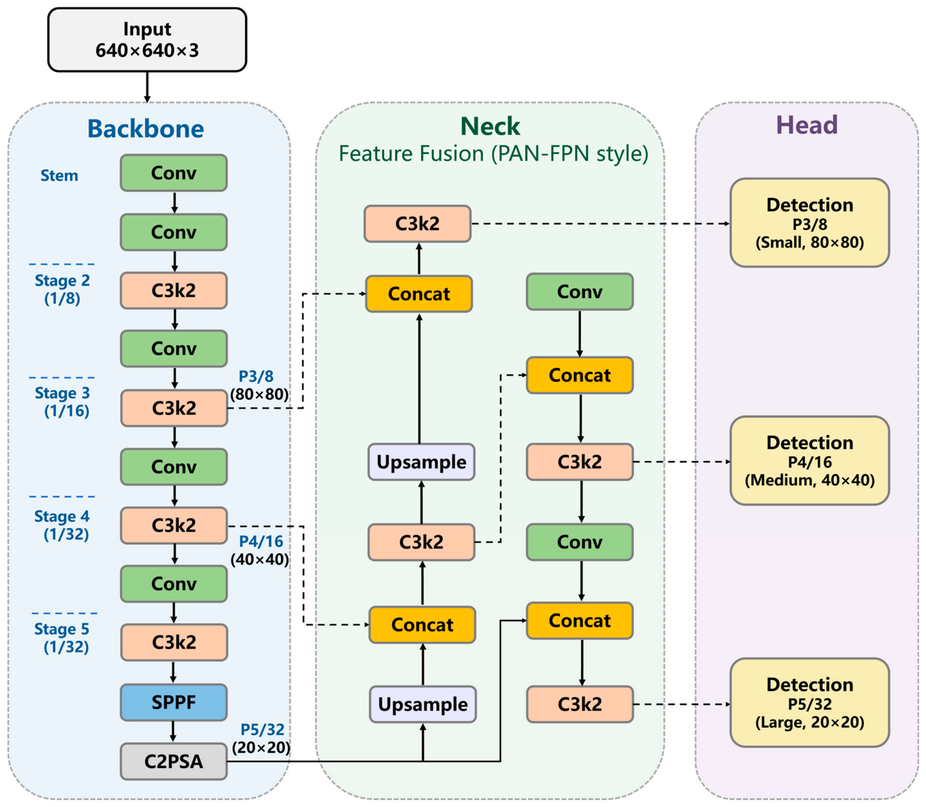
The baseline YOLO11n architecture is shown in Figure 3. It consists of a backbone, a neck, and a detection head. The backbone uses convolutional layers and C3k2 modules to extract features at different depths. An SPPF module near the end of the backbone enlarges the receptive field, and a C2PSA module further strengthens high-level feature representation before feature fusion.
Figure 3.
Baseline YOLO11n architecture used for chopped maize stalk detection.
The neck combines features from different levels through upsampling, concatenation, convolution, and C3k2 modules. This structure allows shallow spatial details and deeper semantic information to be fused before prediction. The detection head produces outputs at three scales, P3, P4, and P5, to detect stalk fragments with different apparent sizes. In the baseline YOLO11n model, the loss function includes classification loss, bounding-box regression loss, and distribution focal loss.
YOLO11n is a practical starting point for this task [24]. Its compact network and multi-scale prediction structure are suitable for images containing several stalk fragments of different sizes. In the proposed framework, however, the detection box is only an intermediate result. The predicted boxes are used to crop local regions for segmentation, skeleton extraction, and length conversion. For this reason, the usefulness of the detector depends on how reliably it localizes complete ROIs, not only on its detection scores.
The baseline model still has limitations when applied to chopped maize stalks. The fragments are usually long and narrow; in this dataset, the mean bounding-box aspect ratio was 8.17. This shape makes box regression more difficult than in compact-object detection tasks. Many fragments also touch or partly overlap, and the boundaries between neighboring stalks are often unclear. Loose fibers, broken edges, and small debris further increase boundary uncertainty. If a predicted box is shifted or truncated, the error can propagate through ROI extraction, segmentation, skeleton extraction, and final length calculation.
2.2.2. Proposed YOLO11n Model
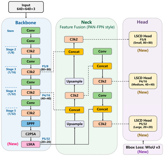
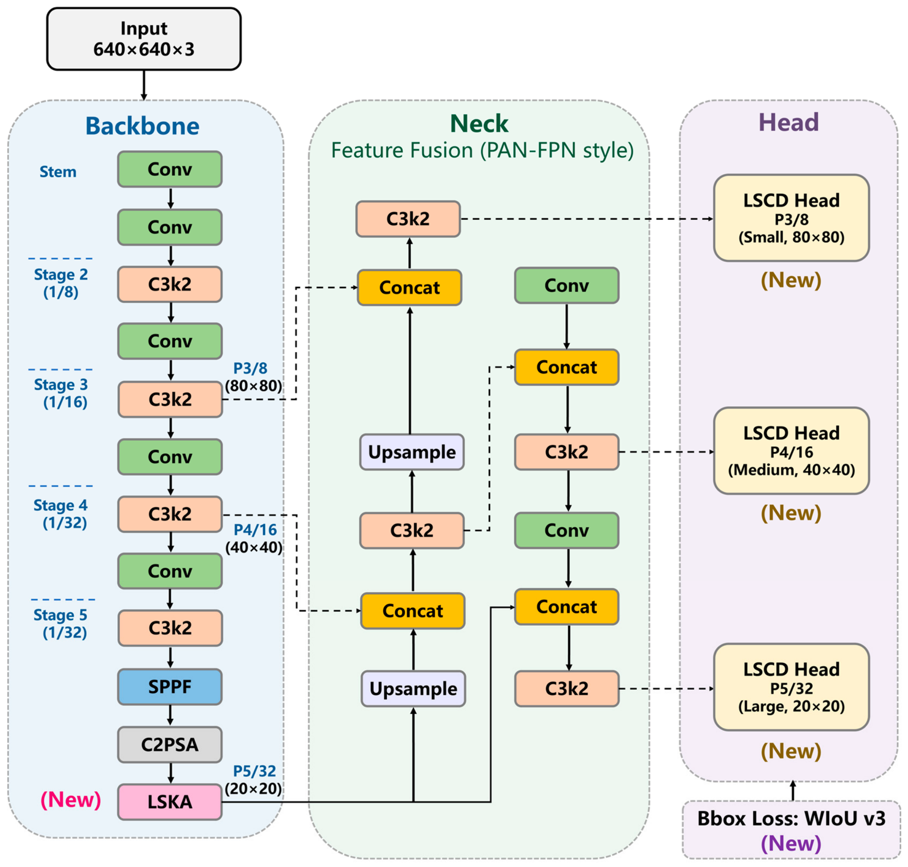
Figure 4 shows the proposed YOLO11n model. The original backbone–neck–head structure was retained, with three modifications for chopped maize stalk detection. An LSKA module was added after C2PSA to enhance the continuity of slender and curved stalk features before feature fusion. The original detection head was replaced with an LSCD head to improve localization consistency across stalk lengths and scales. WIoU v3 was used as the bounding-box regression loss to improve localization stability. In this framework, detected boxes are not final measurement outputs; they define ROIs for segmentation, skeleton extraction, and length calculation. More stable localization at this stage can reduce error propagation in the following measurement steps.
Figure 4.
Proposed YOLO11n architecture with LSKA, LSCD head, and WIoU v3.
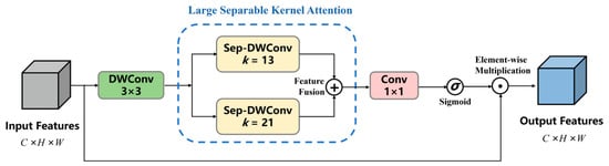
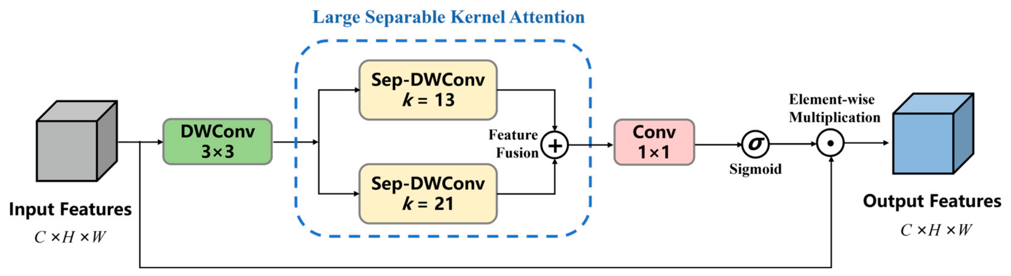
As shown in Figure 5, LSKA was placed after the C2PSA module to enlarge the spatial receptive field before multi-scale feature fusion. Chopped maize stalk fragments are long and narrow, and their visible edges are often interrupted by contact, overlap, broken tips, or loose fibers. A detector that relies mainly on local responses may highlight isolated edge segments rather than the continuous stalk body. LSKA avoids the cost of a full large-kernel depthwise convolution by factorizing a k × k kernel into successive one-dimensional depthwise convolutions, preserving a large receptive field with lower computational and memory cost [25,26]. Similar designs have been used in recent YOLO-based agricultural detection studies to improve feature representation under occlusion, scale variation, and complex backgrounds.
Figure 5.
LSKA module for enhancing slender stalk feature continuity.
For an input feature map X ∈ RC×H×W, a 3 × 3 depthwise convolution first extracts the local feature F0. For a large kernel size k, the separable large-kernel operation is defined as
where Sk(·) denotes the separable depthwise operation with an effective receptive field of k × k. In this study, two kernel sizes were used: k1 = 13 and k2 = 21. The two large-kernel branches were fused and converted into a spatial attention map by a 1 × 1 convolution followed by a sigmoid function:
The output feature was obtained by reweighting the original input feature map:
where A is the spatial attention map, σ(⋅) denotes the sigmoid function, and ⊙ represents element-wise multiplication.
The k1 = 13 branch captures medium-range continuity along the stalk body, whereas the k2 = 21 branch covers a wider spatial range for long and curved fragments. This separable design improves spatial perception without the cost of a full k × k depthwise convolution.
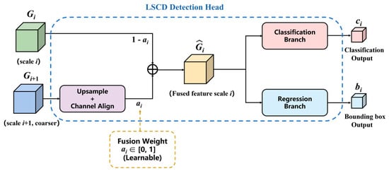
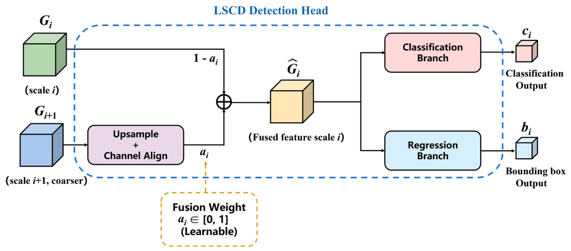
The second modification was made to the detection head. As shown in Figure 6, the standard YOLO11n head was replaced with an LSCD head. Chopped maize stalks vary greatly in length, but their width remains small. This shape variation makes responses across P3, P4, and P5 less stable than in compact-object detection. The LSCD head strengthens the interaction between adjacent detection scales before prediction, allowing local details and deeper semantic information to be better balanced [27,28].
Figure 6.
LSCD head for improving multi-scale stalk localization.
For the i-th detection scale, the adjacent-scale fused feature is written as
where Gi denotes the feature map at the current detection scale, Gi+1 denotes the adjacent coarser-scale feature map, U(⋅) represents upsampling and channel alignment, and αi is a learnable fusion weight. This operation introduces semantic information from the adjacent deeper scale while preserving the spatial details of the current scale.
The fused feature is then fed into decoupled classification and regression branches:
where ci and bi denote the classification output and bounding-box regression output. ψcls(⋅) and ψreg(⋅) represent the classification and regression branches in the detection head.
The LSCD head improves cross-scale localization consistency before prediction. This is important for chopped stalk fragments, whose long and narrow shapes make scale assignment and box localization less stable than in compact-object detection.
The third modification concerns the bounding-box regression loss. WIoU v3 was used because the predicted box serves as the starting point for the later measurement process. In this task, a slightly shifted box may still be counted as a correct detection, but it can crop an incomplete ROI and affect segmentation and skeleton extraction. The regression loss therefore needs to support stable localization, especially for touching, overlapping, and fiber-interfered stalk fragments.
Let Bp and Bg denote the predicted box and the ground-truth box, with center points (xp, yp) and (xg, yg). Let Wc and Hc be the width and height of the smallest enclosing box covering Bp and Bg. The distance-based penalty term is written as
where ε is a small constant used to avoid division by zero. Based on this term, the WIoU v3 regression loss is defined as
where r(β) is the dynamic focusing coefficient, and LIoU is the running mean of the IoU loss. The coefficient r(β) adjusts the contribution of samples with different regression quality, preventing training from being dominated by extremely low-quality boxes or very easy samples.
Compared with the original regression loss, WIoU v3 gives more balanced attention to boxes of different quality. This is useful for chopped maize stalk detection because boundary noise, local overlap, and loose fibers can make some training boxes unstable. By improving box regression stability, WIoU v3 reduces localization errors that would otherwise pass to ROI extraction and later length measurement.
2.3. Detection-Guided Length Measurement
2.3.1. ROI-Based Measurement Workflow
The proposed YOLO11n model outputs bounding boxes for chopped maize stalks and the calibration washer. These boxes are used as localization cues, not as direct measurement results. For chopped stalk fragments, bending, overlap, local occlusion, and small box offsets can make the long side or diagonal of a bounding box inconsistent with the actual fragment length. The predicted boxes were therefore used only to crop ROIs for the subsequent geometric measurement.
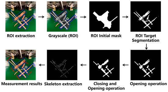
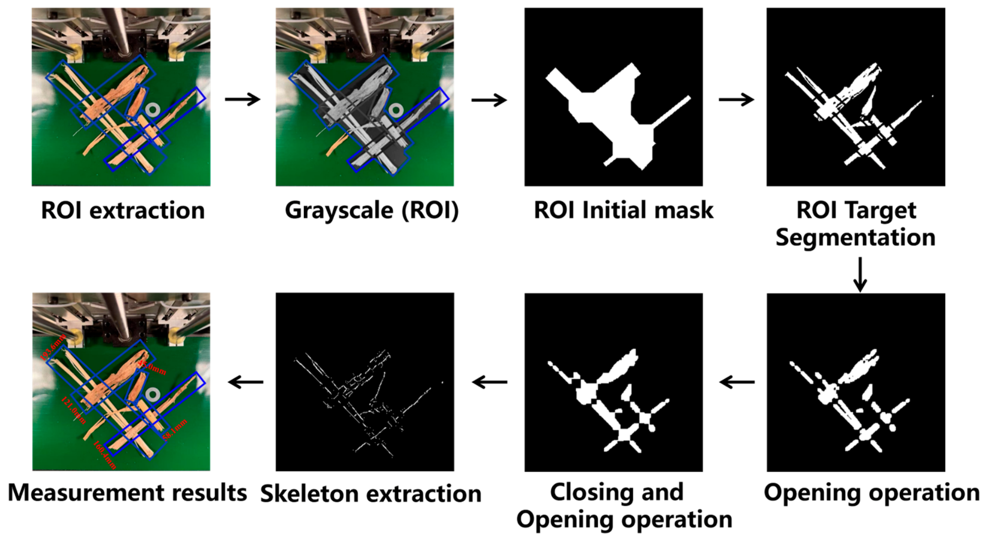
Figure 7 shows the measurement workflow. The stalk and washer ROIs were first extracted from the predicted box coordinates. Each stalk ROI was converted to grayscale and segmented locally to obtain the foreground region. Morphological processing was then applied to remove small disturbances and improve region continuity. The refined binary region was skeletonized, and the main skeleton path was selected to calculate the pixel length of the stalk fragment. Finally, the pixel length was converted to physical length using the scale coefficient obtained from the washer reference.
Figure 7.
Flowchart of chopped maize stalk length measurement based on target detection results.
In this workflow, detection only defines the target region. Length estimation is completed by local segmentation, skeleton extraction, and geometric calculation. This design avoids direct box-based measurement and reduces the influence of bending, overlap, and irregular boundaries.
2.3.2. ROI Segmentation and Mask Refinement
After ROI extraction, the stalk region was separated from the local background before skeleton extraction. Burrs, isolated noise, and small breaks in the binary mask can later become false skeleton branches or incomplete centerlines. Segmentation was therefore performed within each detected ROI rather than on the whole image, which reduced the background area and increased the proportion of the stalk body in the cropped region.
Each ROI was cropped from the original image according to the predicted bounding box and expanded slightly on all sides to reduce boundary truncation. The cropped ROI was converted to grayscale, and Otsu thresholding was applied to obtain an initial foreground mask. Let η denote a candidate threshold. The foreground and background proportions are denoted by pf (η) and pb (η), and their mean gray levels are denoted by μf (η) and μb(η). The between-class variance is defined as
The optimal threshold is obtained by
Using η*, an initial binary mask of the stalk region was obtained. Compared with whole-image thresholding, ROI-based segmentation reduced background interference and kept the mask focused on the detected stalk fragment.
The initial mask still contained small edge burrs, debris, and local discontinuities in some samples. Opening and closing operations were applied in sequence. Opening removed small isolated regions, whereas closing filled minor gaps and improved contour continuity. After morphological refinement, connected-component filtering was used to remove remaining non-target regions. Let the processed binary mask contain K connected regions, denoted by Rk (k = 1, 2, …, K). The retained target region was defined as
where |Rk| is the pixel area of the k-th connected region, and Amin is the minimum area threshold. The retained region R* was then used for skeleton extraction in the next step.
2.3.3. Skeleton Extraction and Length Measurement
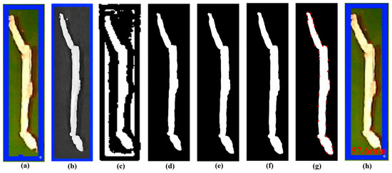
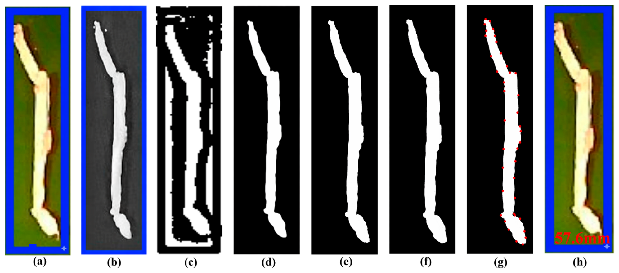
After mask refinement, the stalk region was thinned into a one-pixel-wide skeleton. For chopped maize stalks, neither the long side of the detection box nor the straight-line distance between endpoints can describe the actual length well, especially when the fragment is bent. The skeleton was used as the centerline representation of the stalk body. A representative example is shown in Figure 8. After ROI segmentation and morphological refinement, the stalk contour remained sufficiently continuous for skeleton extraction.
Figure 8.
Example of skeleton-based length measurement for a single chopped maize stalk: (a) ROI extraction; (b) grayscale ROI; (c) ROI mask; (d) segmentation in ROI; (e) opening operation; (f) closing and opening operation; (g) skeleton extraction; (h) measurement result.
The skeleton of an ideal single stalk should form one continuous path. In actual samples, short residual branches may remain because of edge burrs, local contour irregularities, or small noise regions. Counting all skeleton pixels directly can therefore overestimate length. Before length calculation, the skeleton was pruned. Endpoints were identified using the 8-neighborhood rule: a skeleton pixel was defined as an endpoint when it had only one neighboring skeleton pixel. Branches shorter than the preset threshold were removed before the main path was selected [29,30].
Let the pruned skeleton contain Q endpoints, denoted by E = {e1, e2, …, eQ}. For any two endpoints eu and ev, let Puv denote the connected skeleton path between them. If this path contains Nuv ordered skeleton pixels with coordinates (mjuv, njuv), where j = 1, 2, …, Nuv, the pixel length of the path is calculated as
This expression sums the Euclidean distance between adjacent skeleton pixels. The step length is 1 for horizontal or vertical connections and for diagonal connections. Compared with the straight-line distance between two endpoints, this path-based calculation better follows the curved shape of the stalk fragment.
The main stalk body was assumed to correspond to the longest continuous skeleton path. The pixel length of the fragment was defined as
where lp is the final pixel length and P* is the selected main skeleton path. The calculation was based on this main path rather than on the whole skeleton, which may contain residual branches.
The same settings for ROI expansion, thresholding, morphological processing, skeleton extraction, endpoint detection, branch pruning, and main-path selection were applied to all samples. After the pixel length lp was obtained, the physical length lm was calculated using the scale conversion in Equation (2). Algorithm 1 summarizes the complete detection-guided length measurement procedure, and Table 1 lists the parameter settings used in the pipeline.
| Algorithm 1. Detection-guided length measurement of chopped maize stalk fragments. |
| Input: Original RGB image; trained proposed YOLO11n model; true washer inner diameter d0. Output: Physical length lm for each detected chopped maize stalk fragment. |
| 1. Detect chopped maize stalk fragments and the calibration washer using the trained proposed YOLO11n model. |
| 2. Locate the washer ROI and calculate the scale coefficient ks from the washer pixel diameter dp according to Equation (1). |
| 3. For each detected stalk bounding box: |
| 3.1 Crop the stalk ROI with the preset expansion margin. |
| 3.2 Obtain the refined target region R* by ROI segmentation, morphological refinement, and connected-component filtering according to Equation (12). |
| 3.3 Extract and prune the skeleton of R*. |
| 3.4 Determine the main skeleton path P* according to Equations (13) and (14). |
| 3.5 Set the length of P* as the pixel length lp. |
| 3.6 Convert lp to the physical length lm according to Equation (2). |
| 4. Return lm for each detected chopped maize stalk fragment. |
Table 1.
Parameter settings for the measurement pipeline.
3. Experiments
3.1. Experimental Environment
Experiments were conducted on a Windows 11 workstation equipped with an Intel Core i5-13500 CPU(Intel Corporation, Santa Clara, CA, USA), 16 GB RAM, and an NVIDIA GeForce RTX 4060 Ti GPU with 8 GB VRAM. Models were trained and tested in Python v3.10 with PyTorch v2.0. OpenCV v4.8.0 and NumPy v1.24.3 were used for ROI processing, mask refinement, skeleton extraction, and length measurement.
All models were trained and evaluated using the same dataset split, input size, and evaluation protocol. Model-specific default settings were retained where needed. For the proposed YOLO11n-based model, WIoU v3 was used as the bounding-box regression loss. Table 2 lists the main training and inference settings.
Table 2.
Main training and inference settings.
3.2. Evaluation Metrics
The proposed method was evaluated in terms of object detection, length measurement, model complexity, and inference efficiency. Detection metrics assessed whether the model could locate chopped maize stalks and the calibration washer, whereas measurement metrics compared the vision-based length estimates with manual reference values.
For object detection, precision, recall, mAP@0.5, and mAP@0.5:0.95 were used as the main accuracy metrics. Params, FLOPs, and FPS were used to describe model scale and inference efficiency. FPS was measured with a batch size of 1 under the hardware environment described in Section 3.1. Only front-end detector inference time was counted; ROI segmentation, skeleton extraction, and length conversion were excluded.
Let TP, FP, and FN denote the numbers of true positives, false positives, and false negatives, respectively. Precision and recall are defined as
Precision describes the proportion of correct detections among all predicted targets, and recall describes the proportion of true targets that were detected. Based on the precision-recall curve, the average precision (AP) for class c and the mean average precision (mAP) over all classes at a given IoU threshold t are calculated as
where Pc(R, t) denotes the precision of class c at recall level R under the IoU threshold t, and C is the number of object classes.
AP was computed as the area under the discrete precision-recall curve. The stricter COCO-style mAP was calculated by averaging mAP values over IoU thresholds from 0.50 to 0.95 at intervals of 0.05:
In this study, mAP@0.5 evaluates detection at an IoU threshold of 0.5, whereas mAP@0.5:0.95 provides a stricter assessment across multiple IoU thresholds. Because the detection task contained only two visually distinct classes, chopped maize stalk and calibration washer, the main bottleneck was not class confusion. Missed detections and localization instability of slender or overlapped stalk fragments were more important. Recall, strict-IoU AP metrics, and final length-measurement errors were therefore used as the main basis for evaluating the proposed method.
For length measurement, the vision-based results were compared with manual measurements. Let Ai denote the manual length of the i-th sample, Pi denote the predicted length, and N denote the number of evaluated samples. Bias, MAE, and RMSE are defined as
To compare errors across fragments of different lengths, relative error (RE) was also used:
The mean, standard deviation, median, and 90th percentile of RE were reported to describe both the overall error level and the dispersion of the measurement results.
3.3. Comparative Experiments
The proposed model was compared with YOLOv8n, YOLO11n, YOLOv10n, YOLO12n, RT-DETRv2-R18, D-FINE-N, and DEIM-N [31,32,33,34,35,36]. The comparison included YOLO-series detectors, a DETR-based detector, and two recent non-YOLO lightweight detectors. All models were trained and evaluated using the same dataset split, input size, experimental environment, and evaluation protocol. Precision, recall, mAP, and FPS are reported as the mean ± standard deviation over three runs. Params and FLOPs are reported as fixed model attributes. FPS was measured with a batch size of 1 and refers only to front-end detector inference; ROI segmentation, skeleton extraction, and length conversion were excluded.
Table 3 compares the detection accuracy and computational efficiency of the different detectors. Among the YOLO-series baselines, YOLO11n provided a stronger starting point than YOLOv8n, increasing recall from 85.5% to 88.2% and mAP@0.5:0.95 from 64.5% to 68.1%, while using fewer parameters and lower FLOPs. YOLOv10n achieved the lowest Params and FLOPs and the highest FPS, but its recall and mAP@0.5:0.95 were lower than those of YOLO11n, indicating that speed alone did not provide more stable ROI localization.
Table 3.
Detection performance and computational efficiency of different detectors.
The non-YOLO lightweight detectors also achieved competitive accuracy, but at higher computational cost. D-FINE-N and DEIM-N reached mAP@0.5:0.95 values of 70.7% and 70.6%, respectively, but required higher FLOPs and had lower FPS than the proposed model. RT-DETRv2-R18 obtained the highest mAP@0.5 and mAP@0.5:0.95, but its computational cost was much higher, with 20.1 M parameters, 57.4 G FLOPs, and an inference speed of 58 FPS.
The proposed model achieved the highest recall (90.4%) among all compared detectors and maintained a high mAP@0.5:0.95 of 71.1% with 174 FPS. This balance is important for the proposed measurement pipeline, where the detected boxes must provide complete and stable ROIs for later segmentation and skeleton extraction. Additional AP metrics under stricter IoU thresholds and different apparent object sizes are reported in Table 4.
Table 4.
Additional AP metrics of different detectors on the test set.
Table 4 reports additional AP metrics under stricter IoU thresholds and different apparent object sizes. Compared with the baseline YOLO11n, the proposed model increased AP@0.75 from 84.2% to 88.6% and AP@0.95 from 23.6% to 34.1%. These gains indicate improved localization stability under stricter overlap requirements, which is important because inaccurate or truncated boxes can affect ROI segmentation and skeleton extraction.
The proposed model also achieved the highest APs (68.9%) and a high APl (76.6%), showing good adaptability to both small fragments and large stalk targets. RT-DETRv2-R18 obtained the highest AP@0.75, AP@0.95, and APl, and D-FINE-N achieved the highest APm. However, these gains came with higher computational cost or lower inference speed, as shown in Table 3. Among the lightweight detectors, the proposed model provided a favorable balance between strict-IoU localization accuracy, scale-specific detection performance, and inference efficiency. This balance is more suitable for a measurement pipeline in which detection is followed by ROI segmentation and skeleton-based length calculation.
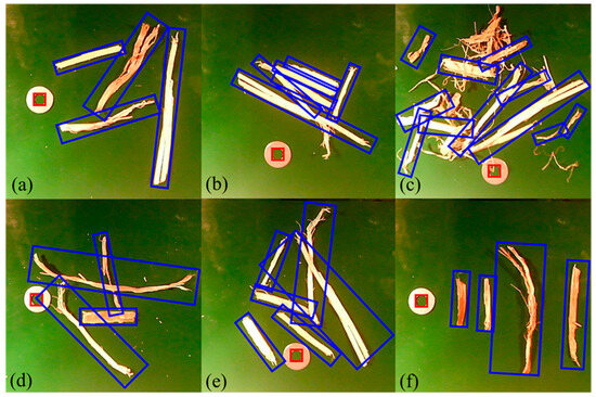
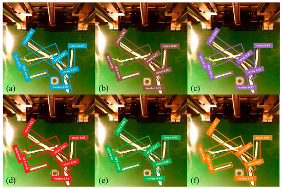
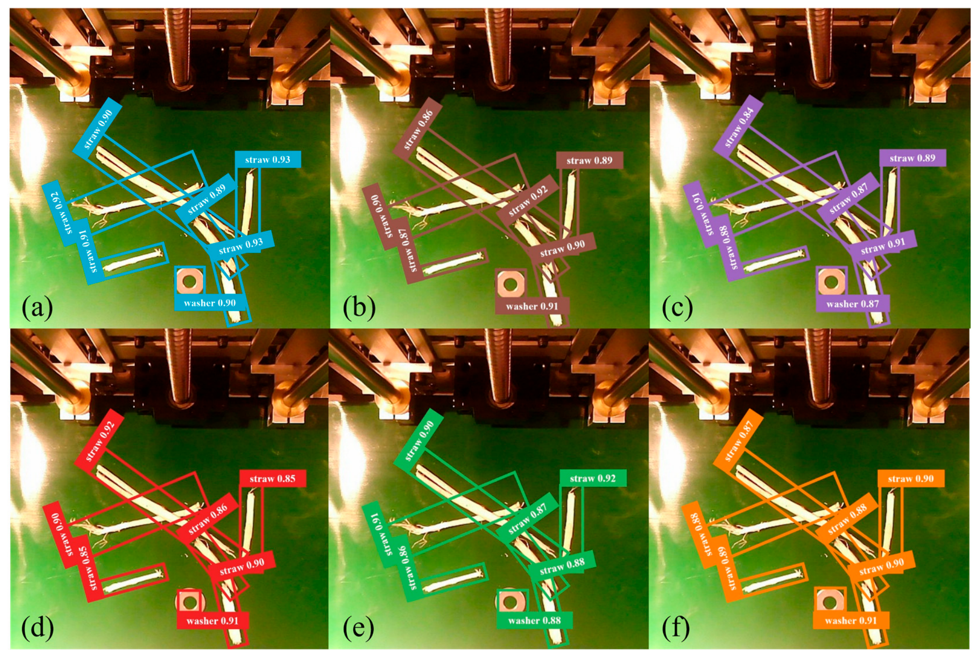
Figure 9 shows representative detection results from six selected models. YOLOv8n and YOLOv10n are omitted from the figure to keep the visual comparison concise, but their quantitative results are reported in Table 3 and Table 4. Differences among the models were most evident in touching, overlapping, and fiber-interfered regions. The proposed model produced fewer missed detections and more complete boxes for slender fragments, which helped provide more reliable ROIs for the subsequent segmentation and skeleton-extraction steps.
Figure 9.
Detection results of different models on representative test samples: (a) proposed model; (b) YOLO12n; (c) RT-DETRv2-R18; (d) YOLO11n; (e) D-FINE-N; (f) DEIM-N.
3.4. Ablation Experiments
Ablation experiments were conducted on the YOLO11n baseline to examine the effects of LSKA, LSCD, and WIoU v3. Each module was added individually and in combination with the others under the same dataset split and evaluation protocol. Precision, recall, mAP, and FPS are reported as the mean ± standard deviation over three runs, whereas Params and FLOPs are fixed model attributes. Because the length-measurement stage depends on the predicted ROIs, recall and mAP@0.5:0.95 were given particular attention.
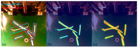
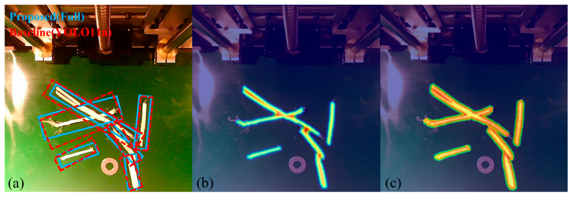
Representative detection results and feature responses are shown in Figure 10. Figure 10a compares the detection boxes of the YOLO11n baseline and the full model on the same sample. Figure 10b,c show the feature-response maps after introducing LSKA and LSCD, respectively. The maps were obtained by normalizing activation maps from the corresponding module outputs, allowing the response regions to be compared visually.
Figure 10.
Visual illustration of the ablation modules: (a) detection results of the YOLO11n baseline and the full model; (b) feature response after introducing LSKA; (c) feature response after introducing LSCD.
The single-module ablation results show that LSKA, LSCD, and WIoU v3 improved different aspects of detection performance. Adding LSKA increased recall from 88.2% to 88.8% and mAP@0.5:0.95 from 68.1% to 69.2%. The larger gain in the stricter IoU metric suggests that LSKA mainly improved box completeness and localization. This effect is consistent with the shape of chopped maize stalks. The fragments are long and narrow, and their visible edges are often interrupted by contact, broken tips, or loose fibers. A detector relying mainly on local features may respond to separated edge segments rather than the whole stalk body. By introducing wider spatial context, LSKA helps connect these local responses and better follows the direction of slender or curved fragments, as shown in Figure 10b.
LSCD had a stronger effect on recall. When used alone, it increased recall from 88.2% to 89.4%, the largest single-module gain for this metric. This indicates that some missed detections in the baseline model were related to unstable scale responses. In the dataset, stalk fragments varied greatly in length while remaining narrow. Some fragments were therefore difficult to represent at a single detection scale, especially when long and short fragments appeared together. LSCD strengthened information exchange between adjacent detection scales, allowing the detection head to combine local details with deeper semantic information before prediction. As a result, it recovered more targets and increased mAP@0.5:0.95 to 69.5%. The feature response in Figure 10c also shows more complete responses for fragments with different lengths and orientations.
WIoU v3 mainly affected bounding-box regression. Because it only replaced the regression loss, Params, FLOPs, and FPS remained unchanged. Precision, recall, and mAP@0.5 changed only slightly, whereas mAP@0.5:0.95 increased from 68.1% to 68.9%. For touching, overlapping, or fiber-interfered stalk fragments, object boundaries are often uncertain, and some training boxes are harder to regress accurately. WIoU v3 reduces the influence of unstable regression samples and gives more balanced attention to boxes of different quality, making its effect more visible under stricter IoU thresholds. This matters for length measurement because even a small box shift can crop an incomplete ROI and affect the subsequent skeleton path.
The two-module results show complementary effects among the three modifications. Combining LSKA and LSCD increased recall to 89.7% and mAP@0.5:0.95 to 70.3%, exceeding the results obtained with either module alone. This pattern suggests that spatial continuity and cross-scale response were separate bottlenecks in chopped stalk detection. LSKA helped the model follow the continuous body of slender and curved fragments, whereas LSCD improved responses to targets with different apparent lengths and scales. Adding WIoU v3 to LSKA or LSCD further improved the stricter localization metric. When LSCD was absent, however, the recall gain remained limited, indicating that regression refinement can improve box quality but cannot fully recover targets that are weakly activated or missed by the detection head.
With all three modules, the model achieved 94.8% precision, 90.4% recall, 96.5% mAP@0.5, and 71.1% mAP@0.5:0.95. Compared with baseline YOLO11n, these values increased by 1.1, 2.2, 0.7, and 3.0 percentage points, respectively. The largest gain was observed for mAP@0.5:0.95, followed by recall. For the measurement pipeline, this improvement is relevant because missed fragments cannot be measured, and shifted or truncated boxes may produce incomplete ROIs and unstable skeletons. As shown in Figure 10a, the full model produced more complete boxes for slender fragments and reduced missed or shifted detections in overlapping regions.
The improvement required only a moderate increase in computation. Params increased from 2.9 M to 3.5 M, FLOPs from 7.6 G to 8.6 G, and FPS decreased from 198 to 174. This cost mainly came from LSKA and LSCD, whereas WIoU v3 did not change the inference structure. Together, the three modifications improved spatial continuity, cross-scale response, and box regression stability, providing more reliable ROIs for subsequent segmentation, skeleton extraction, and length calculation.
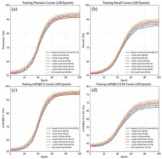
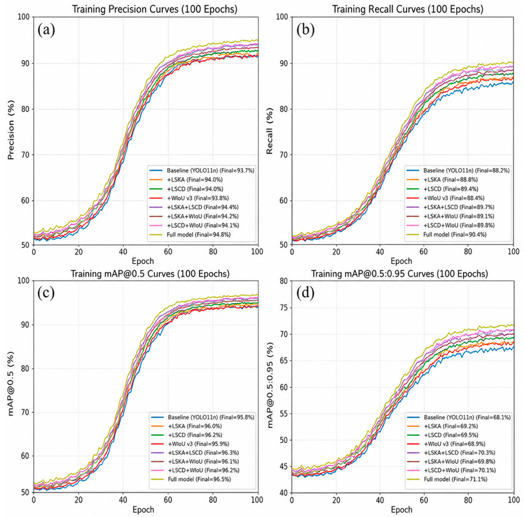
Figure 11 shows representative training curves from one run, whereas the quantitative results in Table 5 are reported as the mean ± standard deviation over three runs. The curves were used to compare the convergence behavior of different ablation settings. In the early epochs, the curves were close to each other. Differences became clearer after the middle stage of training, especially for recall and mAP@0.5:0.95. The full model remained slightly higher in the later epochs and converged without obvious fluctuation. This trend is consistent with Table 5 and supports the complementary effects of LSKA, LSCD, and WIoU v3 on feature continuity, target recovery, and box regression stability.
Figure 11.
Training curves of different ablation settings: (a) precision; (b) recall; (c) mAP@0.5; (d) mAP@0.5:0.95.
Table 5.
Ablation results of the proposed YOLO11n model.
3.5. Length Measurement Accuracy
The accuracy of the proposed measurement pipeline was evaluated by comparing vision-based results with manual reference measurements. Each stalk fragment was measured separately. Straight fragments were measured along the main axis of the dense stalk body, whereas bent fragments were measured by fitting short segments along the main body and summing their lengths. Loose terminal fibers were excluded from the reference measurement. Each fragment was measured three times, and the mean value was used as the final reference length.
A total of 300 stalk fragments were selected from the test set for length-measurement evaluation. The samples were divided into three length ranges: short fragments (<40 mm), medium fragments (40–80 mm), and long fragments (>80 mm), with 100 samples in each group. This grouping was used to examine how measurement error varied with fragment length and shape complexity.
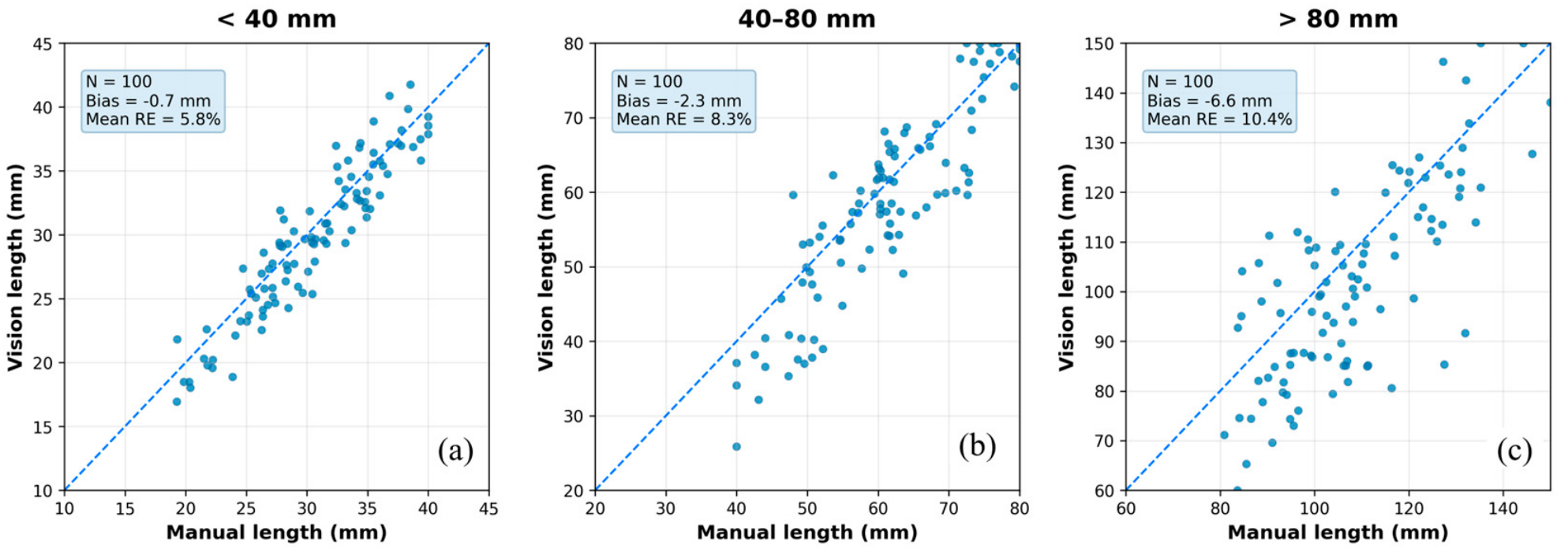
Table 6 shows a slight underestimation across all length ranges. Bias changed from −0.7 mm in the <40 mm group to −2.3 mm in the 40–80 mm group and −6.6 mm in the >80 mm group. MAE, RMSE, and RE followed the same length-related trend. Short fragments were measured more stably, with an MAE of 1.7 mm and a mean RE of 5.8%. For long fragments, MAE increased to 11.2 mm and mean RE to 10.4%, mainly because stronger curvature, local overlap, and incomplete skeleton paths became more common.
Table 6.
Length measurement accuracy in different length ranges.
Large deviations were still limited despite the increase in error with fragment length. No sample in the <40 mm group exceeded 30% RE, whereas one sample in the 40–80 mm group and four samples in the >80 mm group exceeded this threshold. In all three groups, median RE was lower than mean RE, indicating that most fragments had moderate errors and that larger deviations were caused by a small number of long or curved fragments.
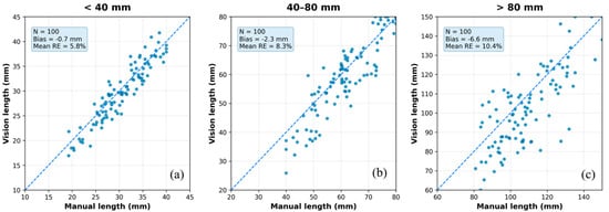
Figure 12 shows the correspondence between manual and vision-based measurements. In all three groups, the points followed the diagonal trend, indicating that the proposed pipeline captured the main variation in stalk length. The scatter gradually widened as fragment length increased. For short fragments, the points were closely distributed around the diagonal, consistent with the small bias and low MAE in Table 6. In the 40–80 mm group, the point cloud became wider and shifted slightly below the diagonal. This underestimation was more evident in the >80 mm group, where the points were more dispersed and more samples fell below the reference line. The pattern agrees with the larger negative bias and higher RMSE observed for long fragments.
Figure 12.
Scatter plots of manual and vision-based length measurements in different length ranges: (a) <40 mm; (b) 40–80 mm; (c) >80 mm.
The relative-error distribution in Table 6 shows the same length-related trend, with higher P90 RE and more high-error cases in longer fragments. This indicates that large errors were concentrated in a small number of long or curved samples rather than distributed evenly across all fragments.
To examine whether the front-end detector affected final measurement accuracy, different detectors were inserted into the same ROI segmentation, skeleton extraction, and length-conversion procedure. The reported processing time includes detector inference, ROI processing, skeleton extraction, and length calculation. The results are shown in Table 7.
Table 7.
Length measurement comparison using different front-end detectors.
Changing the front-end detector changed the final measurement error, although the same segmentation and skeleton-extraction procedure was used. The YOLO11n-based pipeline produced the largest error, suggesting that unstable or incomplete ROIs were passed to the later geometric measurement. YOLO12n reduced the error relative to YOLO11n but still remained behind the proposed method. This result shows that high precision alone is not enough for this task. In skeleton-based length measurement, missed slender fragments and incomplete ROIs are more damaging than small differences in false-positive control.
RT-DETRv2-R18 produced a slightly smaller bias, but its MAE, RMSE, and relative-error statistics were higher than those of the proposed pipeline. Its processing time also increased to 25.1 ms per image. The proposed method gave the lowest overall error, with an MAE of 6.0 mm, an RMSE of 9.4 mm, a mean RE of 8.2%, and five high-error cases. Its runtime was slightly higher than that of the lightweight YOLO baselines but much lower than that of RT-DETRv2-R18.
Overall, Table 7 indicates that the improved detector provided ROIs that were more suitable for skeleton-based measurement. The remaining large errors mainly occurred in long, curved, or locally overlapped fragments, where the foreground mask or the main skeleton path could still be interrupted. To examine the contribution of the post-processing steps, an additional ablation analysis was conducted, as shown in Table 8.
Table 8.
Ablation results of the length measurement pipeline.
Table 8 shows that detection-guided ROI extraction had the largest effect among the tested variants. When whole-image segmentation was used without detection, MAE increased to 14.3 mm and mean RE to 17.8%. Global segmentation could not separate individual stalk fragments reliably when several fragments were close to each other. Loose fibers, broken pieces, and background regions were also more likely to enter the foreground mask. Once included in the skeleton, these non-target regions could connect the main path incorrectly or shift it away from the true stalk centerline.
The post-processing steps also affected skeleton stability. Without ROI expansion, mean RE increased to 10.3%, indicating that some stalk ends were partly truncated when the detected box was close to the object boundary. This problem was more evident for curved or tilted fragments. Removing morphological refinement caused a larger error increase because burrs, gaps, and broken mask regions remained in the foreground and weakened skeleton continuity. Without skeleton pruning, MAE and RMSE also increased, showing that short residual branches from edge noise or contour irregularities could disturb longest-path calculation. The full pipeline achieved the lowest error, with an MAE of 6.0 mm and a mean RE of 8.2%. These results show that stable ROI localization, mask refinement, and skeleton pruning are all needed for reliable length measurement.
A further parameter comparison was conducted to check whether the selected post-processing settings were robust. The tested values, selected values, and stable ranges are summarized in Table 9.
Table 9.
Parameter comparison of key post-processing settings.
The parameter comparison shows that the selected settings balanced stalk-contour retention with suppression of non-target interference. A small ROI expansion was more likely to truncate stalk ends, whereas a larger expansion could introduce nearby fragments or loose fibers. For morphological refinement, small and medium kernels removed burrs and filled minor gaps, but larger kernels could alter the contours of slender stalks. The minimum area threshold removed small debris without discarding valid short fragments. The branch-pruning threshold also needed to remain moderate: a low value retained false branches, whereas a high value could remove part of a true curved end. The final settings were therefore selected from stable ranges rather than from a single isolated minimum.
3.6. Typical Cases and Error Analysis
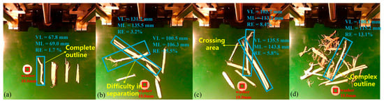
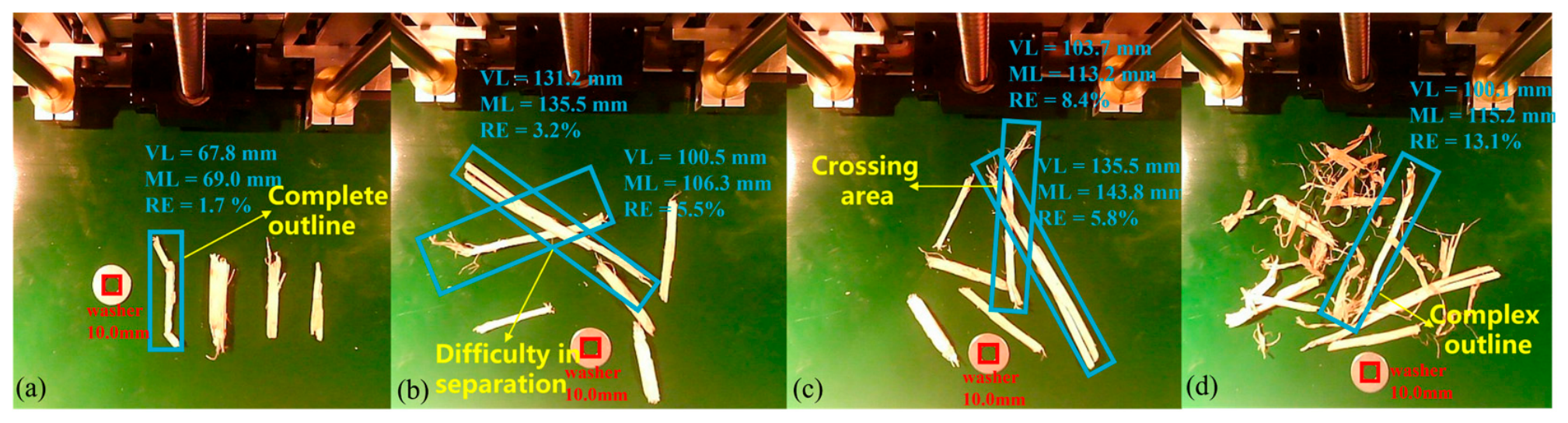
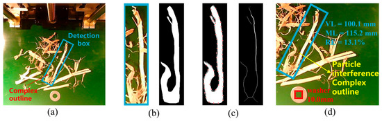
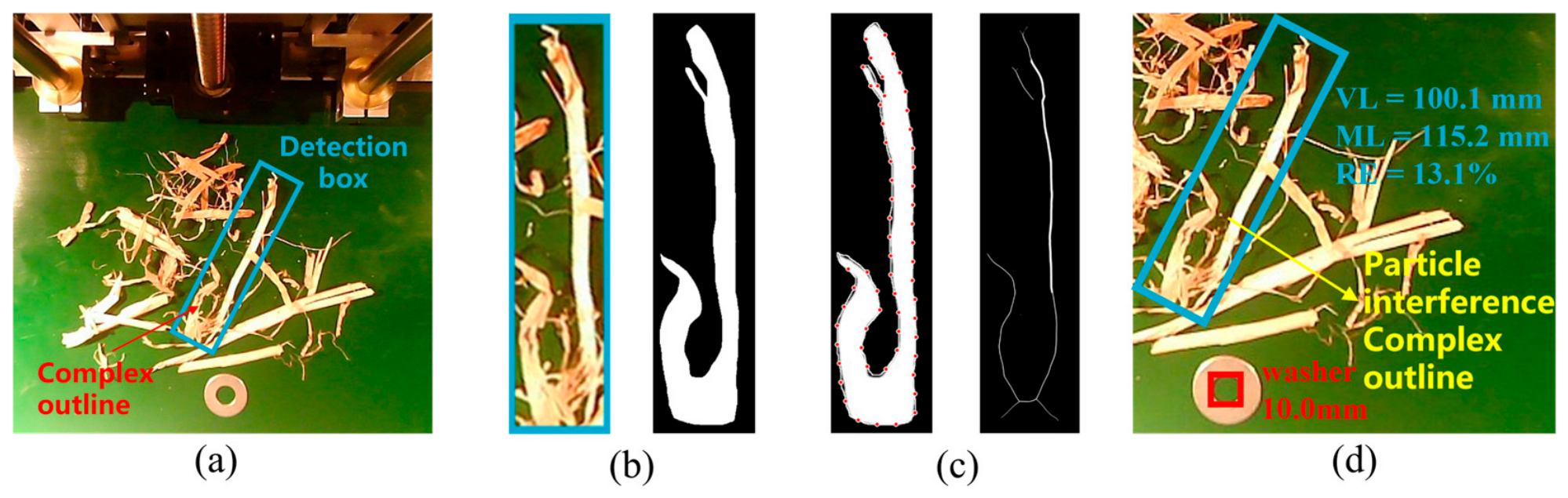
Representative cases were selected from the test set to examine how measurement errors appeared under typical sample conditions. Figure 13 includes sparse fragments, touching fragments, curved-crossing fragments, and cluttered fragments. These cases were not used as predefined scene categories for statistical evaluation. Instead, they illustrate common error sources in the measurement process, including contour discontinuity, local contact, curvature, crossing, and background clutter. Figure 14 further shows the intermediate outputs of one difficult sample, from detection and ROI extraction to skeleton-based length calculation.
Figure 13.
Representative measurement cases under different sample conditions: (a) sparse fragments; (b) touching fragments; (c) curved-crossing fragments; (d) cluttered fragments.
Figure 14.
Intermediate outputs of a representative complex sample: (a) original image and detected bounding box; (b) ROI and segmentation result; (c) skeleton extraction and main path; (d) final length measurement result.
Measurement was most stable when stalk fragments were clearly separated. In the sparse-fragment case, the target contour was complete, and the extracted skeleton followed the main stalk body well. The vision-based length was 67.8 mm, close to the manual reference of 69.0 mm, with a relative error of 1.7%. When adjacent fragments touched each other, the targets could still be detected, but the boundary between fragments became less clear. In Figure 13b, the two examples had relative errors of 3.2% and 5.5%, indicating that local contact had begun to affect contour separation and skeleton-path extraction.
Larger errors appeared when bending, crossing, and clutter occurred together. In Figure 13c, the crossing region weakened local contour continuity, making the extracted skeleton path more likely to deviate from the true stalk axis. The two examples had relative errors of 8.4% and 5.8%, respectively. The largest error among the representative cases occurred in the cluttered-fragment case. In Figure 13d, broken stalk pieces and fiber-like structures around the target disturbed the foreground contour, and the selected main skeleton path became shorter than the actual stalk body. The vision-based length was 100.1 mm, whereas the manual reference was 115.2 mm, giving a relative error of 13.1%. These cases are consistent with Section 3.5, where larger errors were mainly associated with long, curved, crossing, or locally cluttered fragments.
These cases show that measurement stability decreased as fragment arrangement became more complex. Sparse fragments usually had complete contours, allowing the extracted skeleton to follow the stalk body. In touching, curved-crossing, and cluttered cases, nearby fragments, broken edges, and fiber-like structures were more likely to enter the ROI. These factors did not always prevent detection, but they reduced the reliability of the subsequent mask and skeleton.
The main failure patterns were missed detections and shifted or truncated boxes. Missed detections usually occurred when slender fragments were strongly overlapped, partly hidden, or mixed with fiber-like debris. Once missed, a fragment could not enter the measurement process. Shifted or truncated boxes were less severe, but they could still crop incomplete ROIs and affect segmentation and skeleton extraction. For this task, detector robustness therefore depends not only on detection accuracy, but also on whether the predicted ROI is complete enough for length calculation.
Figure 14 illustrates this error transfer in one difficult sample. The detection box covered the target stalk but also included nearby broken pieces and fibers. After segmentation, the main stalk region was retained, but local debris and weak boundaries made the contour less smooth. These defects were carried into the skeleton, producing short residual branches and local path deviations. The selected main path therefore became shorter than the actual centerline, leading to length underestimation.
The remaining errors were not caused solely by detection failure. Instead, small deviations accumulated during ROI extraction, segmentation, skeleton extraction, and longest-path selection. For long, bent, crossed, or cluttered fragments, the key difficulty was maintaining a continuous foreground mask and selecting a skeleton path that followed the real stalk centerline. In the collected samples, bending, overlap, and fiber interference appeared together as natural variations rather than separately controlled factors. The representative cases therefore help explain why errors increased in complex samples and why ROI expansion, mask refinement, and branch pruning were important for stable length measurement.
4. Discussion
The results show that chopped maize stalk length should not be estimated from detection boxes alone. A bounding box can locate a fragment, but it cannot represent the true path length of slender, curved, touching, or overlapped stalks. The proposed framework therefore separates localization from measurement: the detector provides ROIs, and the final length is obtained through ROI segmentation, skeleton extraction, and path-based calculation. This design makes ROI completeness critical, because localization errors can propagate into the subsequent skeleton-based measurement.
Recent image-based studies have provided useful references for this work. Crop-residue measurement studies have used image processing to estimate particle shape and particle-size distribution, but they generally focus on size classification or distribution statistics rather than the physical path length of individual chopped fragments [8,9]. Plant morphology and skeleton-based studies have shown that skeleton extraction can describe elongated biological structures, but their targets are usually intact plant organs or controlled rod-like objects rather than short, broken, touching, and overlapped stalk residues [10,11,12]. Recent YOLO-based agricultural detectors have improved target localization under occlusion, scale variation, and complex backgrounds [25,26,28]. However, these studies mainly optimize detection performance, whereas the present task requires detection boxes that can provide complete ROIs for subsequent skeleton-based length measurement. The comparison with YOLO-series, RT-DETR-based, and other lightweight detectors further shows that high standalone precision or mAP is not sufficient for this task; recall, strict-IoU localization stability, ROI completeness, and inference efficiency are more directly related to measurement accuracy [31,32,33,34,35,36].
The remaining errors mainly occurred in long, strongly curved, crossed, or cluttered fragments. Although the improved YOLO11n provided more stable ROIs, complex occlusion, local overlap, and fiber-like interference could still affect mask extraction and skeleton-path selection. Adjacent fragments or broken fibers may enter the ROI, causing incomplete masks, residual skeleton branches, path deviation, or shortened main paths. Future work should improve segmentation robustness, optimize skeleton pruning and main-path extraction for overlapped stalks, build datasets with explicit bending, overlap, and fiber-interference annotations, and validate the framework on edge devices under field conditions.
5. Conclusions
This study developed a vision-based framework for measuring chopped maize stalk length under fixed imaging conditions. The framework uses an improved YOLO11n detector to locate stalk fragments and the calibration washer, and then estimates physical length through ROI segmentation, skeleton extraction, longest-path calculation, and washer-based scale conversion. The detector achieved 94.8% precision, 90.4% recall, 96.5% mAP@0.5, and 71.1% mAP@0.5:0.95, with a front-end detection speed of 174 FPS. For length measurement, the mean relative errors were 5.8%, 8.3%, and 10.4% for the <40 mm, 40–80 mm, and >80 mm groups, respectively. Across all evaluated fragments, the complete pipeline achieved an MAE of 6.0 mm, an RMSE of 9.4 mm, and a mean relative error of 8.2%.
These results show that detection-guided skeleton measurement can provide reliable chopped-stalk length estimates under controlled imaging conditions. The method still has several limitations. It has not been fully validated under variable field illumination, vibration, motion blur, or complex backgrounds. Scale conversion also depends on a clearly visible calibration washer, and long, strongly curved, crossed, or cluttered fragments may still produce mask discontinuities and skeleton-path errors. Future work will focus on improving contour refinement, skeleton pruning, and main-path extraction, and on testing the framework under more realistic field conditions.
Author Contributions
Conceptualization, B.C. and F.L.; methodology, B.C. and F.L.; software, B.C. and F.L.; validation, J.F.; formal analysis, Z.X.; investigation, B.C.; resources, J.F.; data curation, B.C.; writing—original draft preparation, B.C.; writing—review and editing, F.L. and Z.X.; visualization, Z.X.; supervision, F.L.; project administration, J.F.; funding acquisition, J.F. All authors have read and agreed to the published version of the manuscript.
Funding
This research was funded by the National Key R&D Program of China, grant number 2022YFD200210202, and the Jilin Province Agricultural Machinery R&D, Manufacturing, Promotion and Application Integration Pilot Project, grant number 3D5260554418.
Data Availability Statement
The data presented in this study are not publicly available at this stage because they are associated with an ongoing funded research project, but they will be available from the corresponding author upon reasonable request after the project is completed and relevant requirements are satisfied.
Conflicts of Interest
The authors declare no conflicts of interest.
Abbreviations
The following abbreviations are used in this manuscript:
| YOLO | You Only Look Once |
| ROI | Region of interest |
| LSKA | Large separable kernel attention |
| LSCD | Lightweight cross-scale decoupled detection head |
| WIoU v3 | Wise intersection over union version 3 |
| IoU | Intersection over union |
| mAP | Mean average precision |
| FPS | Frames per second |
| FLOPs | Floating-point operations |
| NMS | Non-maximum suppression |
| RT-DETRv2 | Real-time detection transformer version 2 |
| MAE | Mean absolute error |
| RMSE | Root mean square error |
| RE | Relative error |
Appendix A. Variable Definitions
Table A1.
Definition of the main variables and symbols used in this study.
References
- Ye, F.; Qin, S.; Li, H.; Li, Z.; Tong, T. Policy-Driven Food Security: Investigating the Impact of China’s Maize Subsidy Policy Reform on Farmer Productivity. Front. Sustain. Food Syst. 2024, 8, 1349765. [Google Scholar]
- Paul, M., Jr.; Nana, I.; Zimmermann, A.; Jafari, Y. Trends and evolution of global value chains in food and agriculture: Implications for food security and nutrition. Food Policy 2024, 127, 102679. [Google Scholar] [CrossRef] [Scilit]
- Vučajnk, F.; Šantavec, I.; Kocjan Ačko, D.; Rakun, J.; Verbič, J.; Bernik, R.; Trdan, S.; Vidrih, M. Increased planting speed did not affect silage and grain yield of maize, while saving seed and energy. Ital. J. Agron. 2020, 15, 1612. [Google Scholar] [CrossRef] [Scilit]
- Lima, L.M.; Bastos, M.S.; Ávila, C.L.S.; Ferreira, D.D.; Casagrande, D.R.; Bernardes, T.F. Factors determining yield and nutritive value of maize for silage under tropical conditions. Grass Forage Sci. 2022, 77, 201–215. [Google Scholar] [CrossRef] [Scilit]
- Vu, V.-D.; Ngo, Q.-H.; Nguyen, T.-T.; Nguyen, H.-C.; Nguyen, Q.-T.; Nguyen, V.-D. Multi-objective optimisation of cutting force and cutting power in chopping agricultural residues. Biosyst. Eng. 2020, 191, 107–115. [Google Scholar] [CrossRef] [Scilit]
- Chidozie, B.; Ramos, A.; Vasconcelos, J.; Pinto Ferreira, L.; Gomes, R. Highlighting sustainability criteria in residual biomass supply chains: A dynamic simulation approach. Sustainability 2024, 16, 9709. [Google Scholar] [CrossRef] [Scilit]
- Bhatt, G.; Upadhyay, A.; Sahoo, K. Biomass supply chain network design: Integrating fixed and portable preprocessing depots for cost efficiency and sustainability. Appl. Energy 2025, 389, 125757. [Google Scholar] [CrossRef] [Scilit]
- Igathinathane, C.; Pordesimo, L.O.; Columbus, E.P.; Batchelor, W.D.; Methuku, S.R. Shape identification and particles size distribution from basic shape parameters using ImageJ. Comput. Electron. Agric. 2008, 63, 168–182. [Google Scholar] [CrossRef] [Scilit]
- Nigon, C.M.; Shinners, K.J.; Friede, J.C. An apparatus and method for evaluating particle-size distribution of small grain crop residues. AgriEngineering 2022, 4, 1016–1029. [Google Scholar] [CrossRef] [Scilit]
- Wu, S.; Wen, W.; Xiao, B.; Guo, X.; Du, J.; Wang, C.; Wang, Y. An accurate skeleton extraction approach from 3D point clouds of maize plants. Front. Plant Sci. 2019, 10, 248. [Google Scholar] [CrossRef] [Scilit] [PubMed]
- Miao, T.; Zhu, C.; Xu, T.; Yang, T.; Li, N.; Zhou, Y.; Deng, H. Automatic stem-leaf segmentation of maize shoots using three-dimensional point cloud. Comput. Electron. Agric. 2021, 187, 106310. [Google Scholar] [CrossRef] [Scilit]
- Zhao, J.; Hou, Z.; Hua, H.; Nie, Q.; Pang, Y.; Ma, Y.; Huang, X. LenRuler: A rice-centric method for automated radicle length measurement with multicrop validation. Plant Phenomics 2025, 7, 100103. [Google Scholar] [CrossRef] [Scilit] [PubMed]
- Gruza, M.; Gąska, P.; Harmatys, W.; Gąska, A. New method for testing the laser tracker length measuring unit using a large-scale horizontal arm CMM and its application for assessing the accuracy of distance measurements. Precis. Eng. 2025, 94, 54–66. [Google Scholar] [CrossRef] [Scilit]
- Cui, F.-Y.; Zou, L.-J.; Song, B. Edge feature extraction based on digital image processing techniques. In Proceedings of the 2008 IEEE International Conference on Automation and Logistics, Qingdao, China, 1–3 September 2008; pp. 2320–2324. [Google Scholar]
- Li, H.; Liang, J.; Wu, R.; Cong, R.; Wu, W.; Kwong, S.T.W. Stereo superpixel segmentation via decoupled dynamic spatial-embedding fusion network. IEEE Trans. Multimed. 2023, 26, 367–378. [Google Scholar] [CrossRef] [Scilit]
- Mozerov, M.G.; Karnaukhov, V.N.; Kober, V.I.; Zimina, L.V. Occlusion handling in depth estimation of a scene from a given light field using a geodesic distance and the principle of symmetry of the view. J. Commun. Technol. Electron. 2024, 69, 29–37. [Google Scholar] [CrossRef] [Scilit]
- More, S.S.; Bansode, R. FCN-YOLOS: An effective deep-learning model for real-time object detection. J. Field Robot. 2025, 42, 4053–4074. [Google Scholar] [CrossRef] [Scilit]
- Qiu, J.; Zhang, W.; Xu, S.; Zhou, H. DP-YOLO: A lightweight traffic sign detection model for small object detection. Digit. Signal Process. 2025, 165, 105311. [Google Scholar] [CrossRef] [Scilit]
- Cao, Y.; Li, C.; Peng, Y.; Ru, H. MCS-YOLO: A multiscale object detection method for autonomous driving road environment recognition. IEEE Access 2023, 11, 22342–22354. [Google Scholar] [CrossRef] [Scilit]
- Wu, W.; Lai, J. Multi camera localization handover based on YOLO object detection algorithm in complex environments. IEEE Access 2024, 12, 15236–15250. [Google Scholar] [CrossRef] [Scilit]
- Terven, J.; Cordova-Esparza, D.-M.; Romero-González, J.-A. A comprehensive review of YOLO architectures in computer vision: From YOLOv1 to YOLOv8 and YOLO-NAS. Mach. Learn. Knowl. Extr. 2023, 5, 1680–1716. [Google Scholar] [CrossRef] [Scilit]
- Xu, J.; Li, Z.; Zheng, Y.; Huang, C.; Gu, R.; Xu, W.; Xu, G. OmniSR: Shadow removal under direct and indirect lighting. In Proceedings of the AAAI Conference on Artificial Intelligence; AAAI Press: Washington, DC, USA, 2025; Volume 39, pp. 8887–8895. [Google Scholar]
- Sun, M.; Zhao, R.; Huang, Z.; Ding, S.; Liu, J. IT-OSE: Exploring optimal sample size for industrial data augmentation. IEEE Trans. Ind. Inform. 2026, 22, 5542–5552. [Google Scholar] [CrossRef] [Scilit]
- Hu, F.; Abula, M.; Wang, D.; Li, X.; Yan, N.; Xie, Q.; Zhang, X. Investigation of an efficient multi-class cotton leaf disease detection algorithm that leverages YOLOv11. Sensors 2025, 25, 4432. [Google Scholar] [CrossRef] [Scilit] [PubMed]
- Wang, Y.; Ouyang, C.; Peng, H.; Deng, J.; Yang, L.; Chen, H.; Luo, Y.; Jiang, P. YOLO-ALW: An enhanced high-precision model for chili maturity detection. Sensors 2025, 25, 1405. [Google Scholar] [CrossRef] [Scilit] [PubMed]
- Lin, X.; Liao, D.; Du, Z.; Wen, B.; Wu, Z.; Tu, X. SDA-YOLO: An object detection method for peach fruits in complex orchard environments. Sensors 2025, 25, 4457. [Google Scholar] [CrossRef] [Scilit] [PubMed]
- Shen, Q.; Zhang, L.; Zhang, Y.; Li, Y.; Liu, S.; Xu, Y. Distracted Driving Behavior Detection Algorithm Based on Lightweight StarDL-YOLO. Electronics 2024, 13, 3216. [Google Scholar] [CrossRef] [Scilit]
- Ning, S.; Tan, F.; Chen, X.; Li, X.; Shi, H.; Qiu, J. Lightweight Corn Leaf Detection and Counting Using Improved YOLOv8. Sensors 2024, 24, 5279. [Google Scholar] [CrossRef] [Scilit] [PubMed]
- Li, C.; Qin, H.; Tang, Y.; Zhao, H.; Pan, S.; Liu, J.; Luo, W. An image-based concrete-crack-width measurement method using skeleton pruning and the edge-OrthoBoundary algorithm. Buildings 2025, 15, 2489. [Google Scholar] [CrossRef] [Scilit]
- Deshpande, V.V.; Piat, R. A skeletonization-based image segmentation algorithm to isolate slender regions in 3D microstructures. Mater. Des. 2025, 252, 113765. [Google Scholar] [CrossRef] [Scilit]
- Ali, M.L.; Zhang, Z. The YOLO framework: A comprehensive review of evolution, applications, and benchmarks in object detection. Computers 2024, 13, 336. [Google Scholar] [CrossRef] [Scilit]
- Wang, A.; Chen, H.; Liu, L.; Chen, K.; Lin, Z.; Han, J.; Ding, G. YOLOv10: Real-time end-to-end object detection. Adv. Neural Inf. Process. Syst. 2024, 37, 107984–108011. [Google Scholar] [CrossRef] [Scilit]
- Tian, Y.; Ye, Q.; Doermann, D. YOLOv12: Attention-centric real-time object detectors. Adv. Neural Inf. Process. Syst. 2025, 38, 78433–78457. [Google Scholar]
- Zhao, Y.; Lv, W.; Xu, S.; Wei, J.; Wang, G.; Dang, Q.; Liu, Y.; Chen, J. DETRs Beat YOLOs on Real-Time Object Detection. In Proceedings of the IEEE/CVF Conference on Computer Vision and Pattern Recognition, Seattle, WA, USA, 17–21 June 2024. [Google Scholar]
- Zhu, X.; Su, W.; Lu, L.; Li, B.; Wang, X.; Dai, J. Deformable DETR: Deformable Transformers for End-to-End Object Detection. In Proceedings of the International Conference on Learning Representations, Virtual, 3–7 May 2021. [Google Scholar]
- Zhang, H.; Li, F.; Liu, S.; Zhang, L.; Su, H.; Zhu, J.; Ni, L.M.; Shum, H.-Y. DINO: DETR with Improved DeNoising Anchor Boxes for End-to-End Object Detection. In Proceedings of the International Conference on Learning Representations, Kigali, Rwanda, 1–5 May 2023. [Google Scholar]

Disclaimer/Publisher’s Note: The statements, opinions and data contained in all publications are solely those of the individual author(s) and contributor(s) and not of MDPI and/or the editor(s). MDPI and/or the editor(s) disclaim responsibility for any injury to people or property resulting from any ideas, methods, instructions or products referred to in the content. |
© 2026 by the authors. Licensee MDPI, Basel, Switzerland. This article is an open access article distributed under the terms and conditions of the Creative Commons Attribution (CC BY) license.