TSN Schedulability Analysis with TAMCQF + CBS for Automotive Ethernet

Abstract

Time-Sensitive Networking (TSN) has emerged as a critical communication protocol for automotive Ethernet to support the high-bandwidth, real-time, and deterministic transmission requirements of next-generation in-vehicle networks. However, a clear and effective TSN mechanism combination tailored to the mixed and bursty traffic characteristics of automotive scenarios remains lacking. To address this issue, this paper proposes a combined TSN scheduling mechanism for automotive scenarios. The highest-priority traffic is scheduled by class-based Time-Aware Shaper (TAS), periodic bursty sensor traffic is shaped by Credit-Based Shaper (CBS), and medium-priority traffic adopts Multi-Cyclic Queueing and Forwarding (MCQF). Based on Compositional Performance Analysis (CPA), this paper derives the worst-case latency upper bound expressions for CQF streams and optimizes the schedulability analysis to reduce conservative errors. Simulation verifies that the theoretically calculated bounds cover the maximum simulation latency, and the optimized analysis reduces conservatism, with peak conservative error of 3.07% in the ring scenario and 10.59% in the automotive scenario. Compared with the strict priority and TAMCQF (a combination of TAS and Multi-CQF), the proposed mechanism combination suppresses the latency jitter of mixed traffic, mitigates long-duration blocking of medium-priority traffic caused by high-priority burst data, and provides reliable deterministic transmission guarantees for automotive in-vehicle networks.

1. Introduction

With the rapid evolution of vehicles toward autonomous driving and full-domain intelligent cockpits, the automotive Electrical/Electronic Architecture (EEA) is iterating from a distributed layout to domain-centralized, zonal, and central computing architectures. The traditional CAN bus can no longer meet the demands of massive sensor data transmission, high-real-time control command interaction, and multi-domain data fusion.

Automotive Ethernet has become the core carrier of the automotive backbone network due to its high bandwidth and strong scalability. As a key enhancement technology for automotive Ethernet, Time-Sensitive Networking (TSN) features four core capabilities—time synchronization, resource management, traffic scheduling and shaping, and reliability—providing high-performance, reliable, and real-time communication for in-vehicle networks. The traffic scheduling and shaping sub-protocols of the TSN include several specifications that guarantee link-layer Quality of Service (QoS). For instance, IEEE 802.1Qch specifies the Cyclic Queueing and Forwarding (CQF), which configures two queues on switch ports to alternately perform enqueueing and dequeueing operations. It ensures frames received in one time interval are transmitted in the next. IEEE 802.1Qbv defines the Time Aware Shaper (TAS), which employs time-based gating to control traffic of different priorities. It allows frame transmission only when the corresponding gate is open. IEEE 802.1Qav defines the Credit-Based Shaper (CBS), which regulates the transmission bandwidth of target traffic classes and smoothes traffic bursts. Other sub-protocols, such as 802.1Qcr and 802.1Qbu, further support deterministic transmission and bounded latency for automotive Ethernet from various perspectives.

The selection of traffic scheduling and shaping mechanisms has long been a research hotspot, and studies on the hybrid application of TAS and CQF mechanisms have advanced in recent years.

Pei [1] proposed a model combining TAS with a single CQF queue, with the highest-priority traffic scheduled via an independent TAS gate, and priorities 6 and 5 scheduled with CQF. Finn [2] proposed the Multi-CQF (MCQF) mechanism based on CQF, which uses multiple CQF queues with strictly proportional cycle lengths. Compared with the TAS-only scheme, this model improves the capability to transmit mixed traffic. Alexandris [3] compared TAS, CSQF (a three-buffer variant of CQF), and MCQF in industrial scenarios, showing that MCQF performs best under mixed constraints. It satisfies strict latency requirements for critical traffic while accommodating medium- and low-latency traffic. They further suggested scheduling the most critical traffic with TAS and combining it with MCQF to guarantee mixed traffic transmission. Nie [4,5] proposed the TAMCQF model, in which the highest priority 7 is scheduled by TAS, priorities 1–6 are managed by three groups of CQF queues.

On the other hand, bounded latency of traffic in vehicular networks is fundamental for the stable operation of the system. Obtaining the worst-case latency upper bound for target traffic is of great significance for the application of TSN mechanism combinations. Methods to obtain the worst-case latency upper bound for target traffic include simulation methods, model checking methods, and analytical methods [6]. Simulation methods and model checking methods require a significant amount of time to obtain the worst-case result, while analytical methods take less time to compute, but yield more pessimistic and conservative latency results. Compositional Performance Analysis (CPA) is an analytical method that has been applied by multiple studies to analyze the schedulability of TSN mechanisms, including the use of a single mechanism [7,8,9,10,11,12,13] and the combination of multiple mechanisms [14,15,16,17]

The TAMCQF model effectively supports mixed traffic transmission but does not fully account for scenarios involving massive and bursty traffic. With the development of autonomous driving, high-bandwidth sensors such as high-definition cameras and LiDAR periodically generate massive burst data, typically assigned high priorities. Transmitting these data may cause a delay or blockage of tens of milliseconds for medium-priority traffic at a single output port. Although medium-priority traffic has relaxed end-to-end latency requirements, blocking by bursty high-priority traffic across multiple hops can cause accumulated latency to exceed permissible limits.

To address the above limitations of the TAMCQF model and ensure reliable mixed traffic transmission in automotive scenarios, this study proposes a combined mechanism of TAMCQF + CBS and analyzes the schedulability of different traffic classes within this combined model. Furthermore, the effectiveness of the combined mechanism and the correctness of the derived timing analysis expressions are verified through simulation. This research aims to provide guidance on mechanism combinations for applying TSN in automotive Ethernet. The contributions of this paper are as follows:

• Proposes a TAMCQF + CBS mechanism combination applied to automotive scenarios.
• Conducts timing analysis on the proposed mechanism combination and derives upper-bound latency expressions.

2. Materials and Methods

2.1. Mechanism Combination

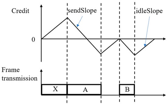
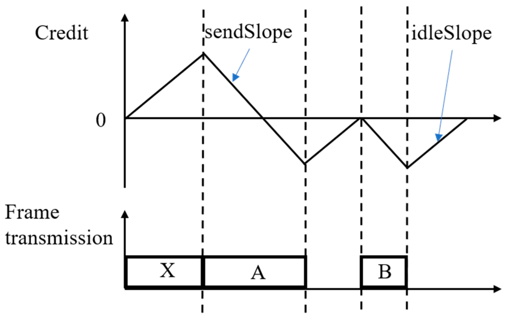
CBS is a transmission selection algorithm applicable to output ports in TSN. The core of the algorithm is to control queue sending using “credit”. Each CBS class independently maintains a credit value. When the queue is idle, the credit increases at an idleSlope rate, and when data is sent, it is deducted at a sendSlope rate, as shown in Figure 1. Messages can only start to be sent when the credit value is non-negative. If the credit is negative, sending is paused and waits for the credit to recover, thus limiting traffic bursts and preventing other traffic from being blocked for a long time. Asynchronous Traffic Shaping (ATS) is another mechanism provided by TSN to limit traffic bandwidth. Combined with flow identification capabilities, it enables precise bandwidth control down to individual streams. However, this mechanism stipulates a maximum residence time, and packets exceeding this time will be discarded. It is not suitable for traffic with strict requirements on the frame packet loss rate [18].

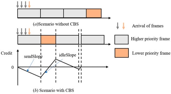
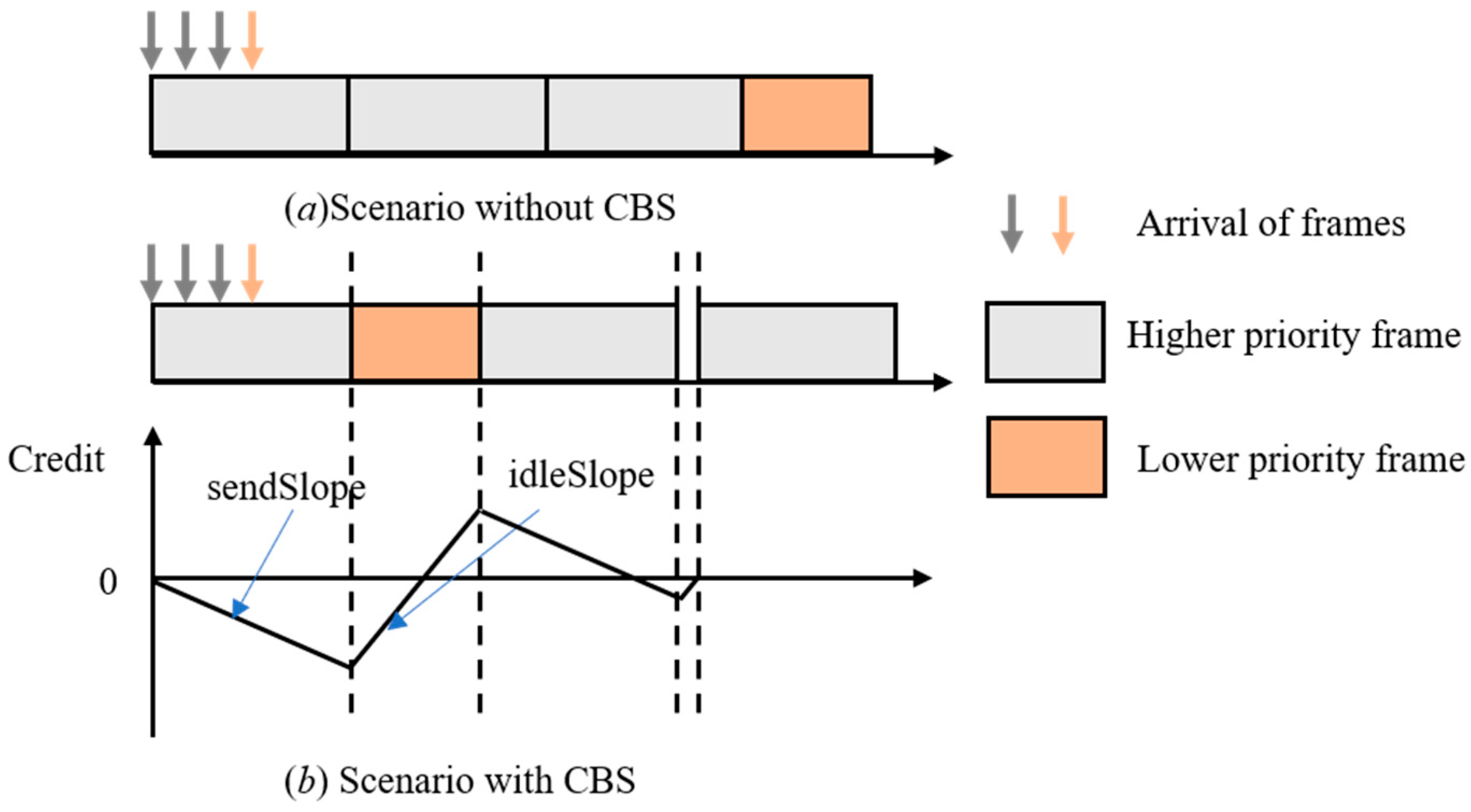
In the vehicular scenario, periodically bursting and massive sensor data may block lower-priority frames, as shown in Figure 2a. With CBS, the transmission of burst traffic can be restricted, as shown in Figure 2b. This type of traffic is subject to credit constraints, resulting in transmission intervals between frames. Frames with lower priority can commence transmission within these intervals. Among the sensor traffic, the message that experiences the greatest overall blocking is the last frame. When the idleSlope parameter of CBS is set to a higher value, this frame can experience less blocking from CBS shaping.

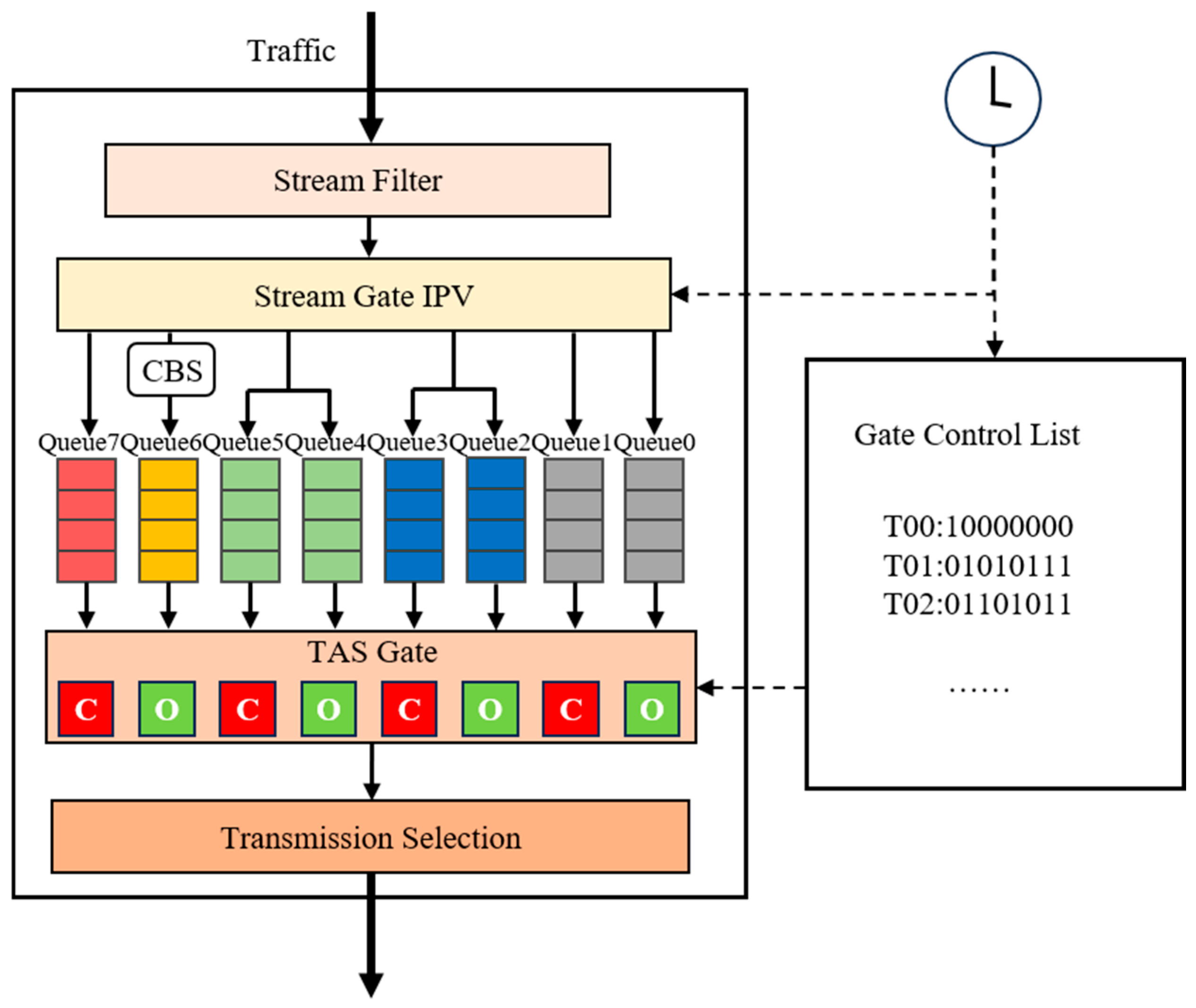
The proposed combined model, as shown in Figure 3, prioritizes the use of TAS for the highest priority level 7, employs the CBS mechanism for the second-highest priority level, utilizes the MCQF scheduling for medium priority levels, and does not employ any mechanism to ensure transmission for priority levels 0–1.

For the highest priority TAS, there are two common application modes: stream-based TAS and class-based TAS [19]. Stream-based TAS requires end stations to support TSN capabilities, including AS and TAS, which most current vehicle ECUs lack, as they typically operate as simple sensors [20]. Abnormal conditions, such as frame loss and synchronization errors, may result in unreliable scheduling outcomes [21]. Stream-based TAS also suffers from design complexity and high memory usage during scheduling. In contrast, class-based TAS offers simpler configuration and greater tolerance for flow jitter at the cost of additional bandwidth requirements [19].

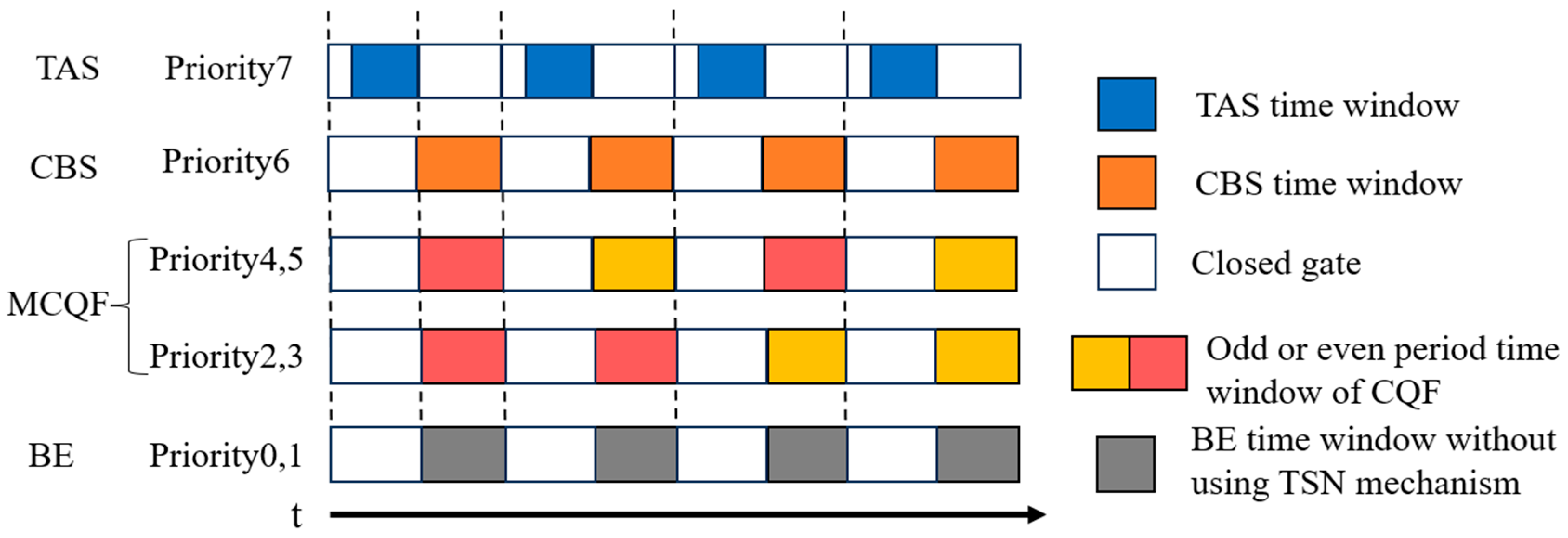
In summary, for the class-based TAS usage method, the timing model of TAMCQF plus CBS is shown in Figure 4. The highest priority is ensured by reserving a TAS time window larger than the actual traffic bandwidth within each TAS cycle. The CBS mechanism is used to spread out periodic bursts of large data traffic. Two sets of CQF queues schedule medium and low priority traffic to achieve deterministic latency and acceptable jitter. Low priority levels 0 and 1 are BE traffic, which is transmitted using gaps in other traffic transmissions, without guaranteeing its latency and packet loss rate.

2.2. Schedulability Analysis

Previous research has derived schedulability expressions for class-based TAS streams and optimized them for multi-hop scenarios [22].

The scenario of the combined use of TAS and CBS has been analyzed in Ref. [17], and the congestion experienced by the CBS stream is given by Equation (7) of the same reference.

Variables used in the analysis of the CQF mechanism are listed in

Table 1. Variable list of CQF stream schedulability analysis.

Variable	Meaning of the Variable
$a_i^q$	Arrival time of the q-th frame of stream i
$A_i^q$	A set of possible values of $a_i^q$ that lead to the worst-case same-priority blocking under First-In-First-Out (FIFO) policy (see Equation (10) in the Ref. [7])
$w_i(q,a_i^q)$	Worst-case queuing delay of the q-th frame of stream i
$C_i^{+}$	Transmission time of the longest frame in stream i
${\eta }_i^{+}\left(\Delta t\right)$	Maximum number of frames of stream i arriving within time interval Δt
$sp\left(i\right)$	Set of traffic with the same priority as stream i
$hp\left(i\right)$	Set of traffic with higher priority than stream i
$I_i^{SPB}$	Maximum blocking from same-priority traffic
$Q_i$	Range of q for stream i, which is a continuous set of positive integers
${R_i}^{+}$	Worst-case response time of stream i at the current egress port
$I_i^{CGB}$	Maximum blocking caused by closed TAS gate
$t_{tas}$	Duration of the gate opening for highest priority 7 within a single TAS cycle
$t_{tascyc}$	Cycle of TAS gate control list
$t_{gb}$	Duration of guard band before the opening of the highest-priority TAS gate
$t_i^{cqf}$	Length of a single odd or even CQF cycle for stream i. 2$t_i^{cqf}$ denotes the full CQF cycle
$I_i^{HPB,CQF}$	Maximum blocking caused by all frames with higher priority than i and using the CQF mechanism
$I_i^{HPB,TAS}$	Maximum blocking caused by all frames with higher priority than i and using the TAS mechanism
$I_i^{HPB,CBS}$	Maximum blocking caused by all frames with higher priority than i and using the CBS mechanism
$F_{TAS}$	Set of traffic using TAS
${CR}_{max}$	Upper limit of the CBS credit bucket

.

The CQF mechanism divides time into equally sized, alternating odd and even time intervals. Frames received during an even time interval are scheduled for transmission in the next odd time interval, and vice versa. The transmission scheduling of a frame is determined solely by the time interval in which it arrives. If the transmission duration of pending frames exceeds the available time interval, transmission in this overloaded interval will continue and extend into the next time interval of the same parity.

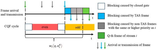
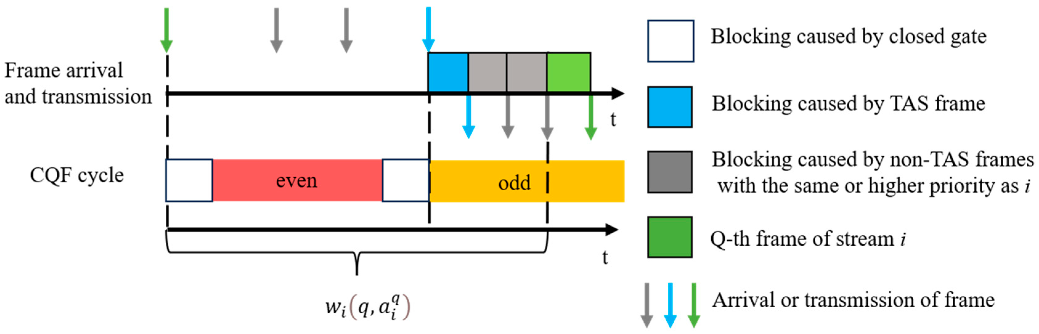
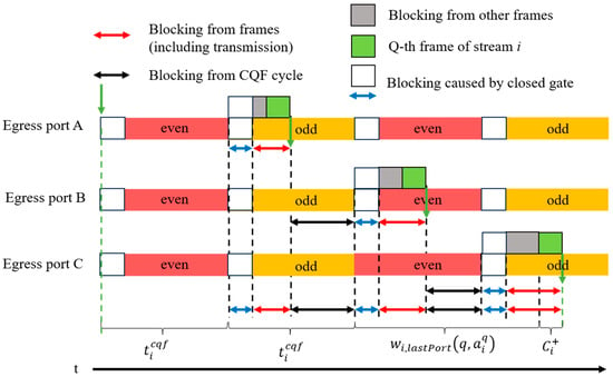
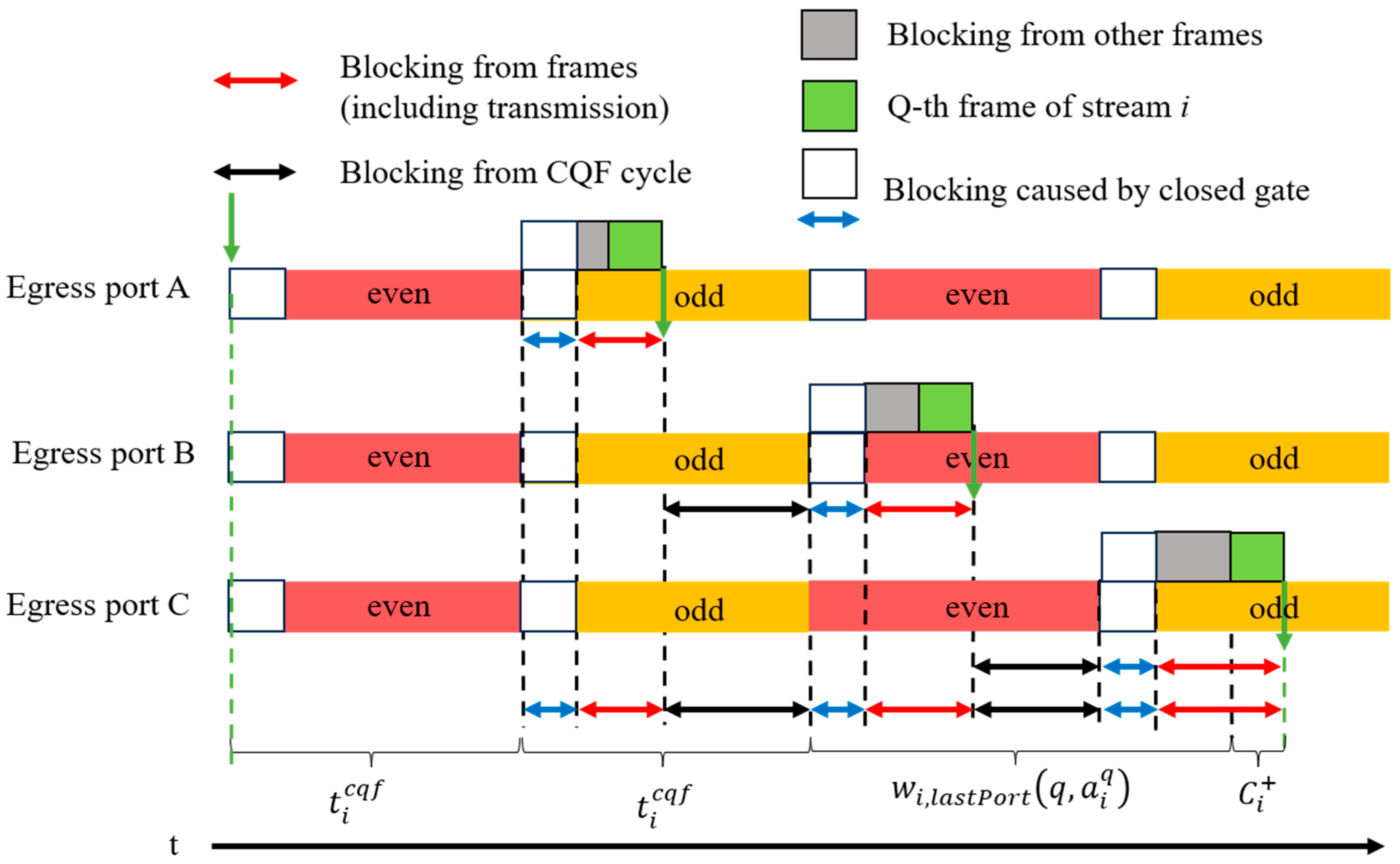
The busy period of CQF traffic, as shown in Figure 5, consists of the following components:

• Blocking caused by the CQF cyclic queuing and forwarding mechanism, denoted as $t_i^{cqf}$.
• Blocking due to gate closure, including time windows exclusively opened for TAS stream and guard band, denoted as $I_i^{CGB}$.
• Blocking caused by TAS frames arriving at the end of a dedicated TAS time window, where the blocking equals the transmission time of the longest TAS frame. The maximum blocking from a TAS frame per TAS cycle is $\underset{j\in F_{\mathit{TAS}}}{\max }\left\{C_j^{+}\right\}$.
• All traffic at the same priority level as stream i (including stream i itself) and high-priority non-TAS traffic. Among these, same-priority blocking is denoted as $I_i^{SPB,CQF}$, high-priority CQF traffic blocking as $I_i^{HPB,CQF}$, and high-priority CBS traffic blocking as $I_i^{HPB,CBS}$.

Therefore, the queuing time expression for the target stream using CQF is given by Equation (1):

$$\begin{array}{cc}\hfill w_i\left(q,a_i^q\right)=& t_i^{cqf}+I_i^{CGB}\left(w_i\left(q,a_i^q\right)-t_i^{cqf}+C_i^{+}\right)+I_i^{SPB,CQF}\left(q,a_i^q\right)\hfill \\ & +I_i^{HPB,CQF}\left(w_i\left(q,a_i^q\right)-t_i^{cqf}+C_i^{+}\right)+\hfill \\ & I_i^{HPB,TAS}(w_i\left(q,a_i^q\right)-t_i^{cqf}+C_i^{+})+I_i^{HPB,CBS}\left(w_i\left(q,a_i^q\right)\right)\hfill \end{array}$$

(1)

To ensure that CQF traffic arriving in the current odd (or even) time interval is transmitted in the next even (or odd) time interval, Equation (1) must also satisfy the condition given in Equation (2).

$$w_i\left(q,a_i^q\right)<2·t_i^{cqf}-C_i^{+}$$

(2)

Low-priority traffic cannot cause the blocking of the target traffic employing the CQF mechanism. It can only block the busy period or queuing time if its transmission starts before the busy period. However, with CQF, any ongoing low-priority packet will complete transmission within the cycle in which the target traffic arrives (e.g., the even cycle in Figure 5).

Blocking caused by gate closure includes blocking from guard band time and the time window exclusively allocated for the TAS stream. This blocking must be calculated once per TAS cycle. Meanwhile, the odd or even CQF time interval during which the target traffic arrives shall be subtracted from the queuing time before being used as the input variable, as shown in Equation (3).

$$I_i^{CGB}\left(w_i\left(q,a_i^q\right)-t_i^{cqf}+C_i^{+}\right)=⌈{\displaystyle \frac{w_i\left(q,a_i^q\right)-t_i^{cqf}+C_i^{+}}{t^{tascyc}-{(t}^{tas}+t^{gb})}}⌉\left(t^{tas}+t^{gb}\right)$$

(3)

When calculating blocking from the same priority, it is necessary to consider the first q − 1 frames of the target stream, and follow the FIFO rule for the same priority. Any frames that arrive after the q-th frame of stream i will not cause blocking during busy time. The blocking from the same priority is shown in Equation (4).

$$I_i^{SPB}\left(q,a_i^q\right)=\left(q-1\right)C_i^{+}+\sum _{j\in sp\left(i\right),i\ne j}\left({\eta }_j^{+}\left(a_i^q\right)C_j^{+}\right)$$

(4)

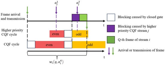
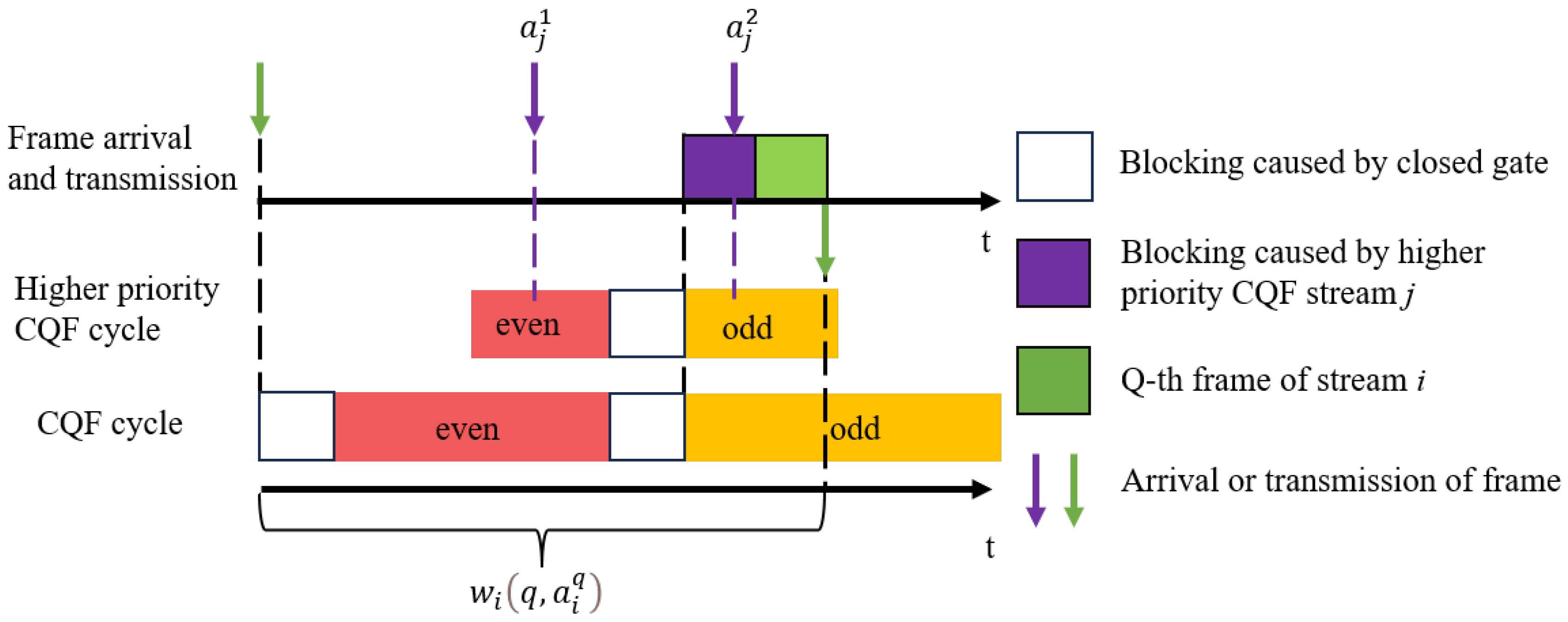
The impact of blocking from the high-priority CQF stream is consistent with Ref. [12]. As shown in Figure 6, in the worst case, high-priority CQF stream j is delayed by one CQF time interval $t_j^{cqf}$ before interfering with frames of stream i. The first purple frame of stream j arriving at time $a_j^1$ is delayed to the next CQF time interval and blocks the queuing time of target stream i. By contrast, the second purple frame of stream j arriving at time $a_j^2$ cannot block the target frame, and must wait until its next even cycle to start transmission. The maximum number of CQF time intervals of stream j within an arbitrary time interval Δt can be calculated using the ceiling operation $⌈{\displaystyle \frac{w_i\left(q,a_i^q\right)-t_i^{cqf}+C_i^{+}}{t_j^{cqf}}}⌉$. Multiplying this number by the duration of the CQF time interval of stream j yields the cumulative time interval of interference from high-priority CQF stream j. This time interval can be used as the input to the arrival function ${\eta }_i^{+}$ to compute the high-priority blocking duration imposed on stream i by each stream j in the CQF class. The final high-priority CQF traffic blocking $I_i^{HPB,CQF}$ is given by Equation (5).

$$\begin{array}{c}{I}_i^{HPB,CQF}\left(w_i\left(q,a_i^q\right)-t_i^{cqf}+C_i^{+}\right)=\\ {\displaystyle \sum _{j\in \left\{k|k\in hp\left(i\right)\cap k\in CQF\right\}}}{\eta }_j^{+}\left(⌈{\displaystyle \frac{w_i\left(q,a_i^q\right)-t_i^{cqf}+C_i^{+}}{t_j^{cqf}}}⌉t_j^{cqf}\right)C_j^{+}\end{array}$$

(5)

Since the TAS mechanism does not add a guard band after the end of the TAS time window, a frame of highest-priority blocking needs to be considered after the end of each TAS time window. This blocking should be the time required for the transmission of the longest frame in the TAS traffic, namely $\underset{j\in hp\left(i\right)}{\max }\left\{C_j^{+}\right\}$, resulting in the maximum highest-priority blocking $I_i^{HPB}\left({s^{\prime }}_i^q+C_i^{+}\right)$ as shown in Equation (6):

$$I_i^{HPB,TAS}\left(w_i\left(q,a_i^q\right)-t_i^{cqf}+C_i^{+}\right)=⌈{\displaystyle \frac{w_i\left(q,a_i^q\right)-t_i^{cqf}+C_i^{+}}{t_{tascyc}}}⌉·\underset{j\in F_{\mathit{TAS}}}{\max }\left\{C_j^{+}\right\}$$

(6)

The maximum number of frames of high-priority CBS traffic j arriving within the queuing time of the target stream is ${\eta }_j^{+}\left(w_i\left(q,a_i^q\right)\right)$. Therefore, without considering credit constraints, the total blocking caused by all CBS traffic is ${\sum }_{j\in hp\left(i\right)\cap j\in CBS}\left({\eta }_j^{+}\left(w_i\left(q,a_i^q\right)\right)C_j^{+}\right)$. Under CBS credit constraints, let x denote the transmission time of CBS traffic within a time interval Δt. The consumed credit is then $x·{\alpha }^{-}$, while the maximum accumulated credit during this interval is $\left(\Delta t-x\right)·{\alpha }^{+}+{CR}_{max}$. It follows that $x\le {(CR}_{max}+\Delta t·{\alpha }^{+})/({\alpha }^{+}+{\alpha }^{-})$. Since the credit of CBS does not increase during gate closure, this duration must be subtracted, yielding Equation (7).

$$\begin{array}{c}{I}_i^{HPB,CBS}\left(w_i\left(q,a_i^q\right)\right)=\\ \min \left\{{\displaystyle \sum _{j\in hp\left(i\right)\cap j\in CBS}}\left({\eta }_j^{+}\left(w_i\left(q,a_i^q\right)\right)C_j^{+}\right),{\displaystyle \frac{{CR}_{max}+{\alpha }^{+}·(w_i\left(q,a_i^q\right)-t_i^{cqf}-I_i^{CGB})}{{\alpha }^{+}+{\alpha }^{-}}}\right\}\end{array}$$

(7)

In summary, the worst-case latency analysis for the CQF stream at a single egress port is completed. CQF needs to be combined with the AS protocol, and the odd-even cycle instants at the egress ports of nodes within the network are aligned. From a global data-link-layer perspective, when the stream satisfies Equation (2), the situation is as shown in Figure 7. Assume ports A, B, and C are three egress ports of switches along the transmission path of stream i. When the green target traffic frame is transmitted through the switch, the sum of the blocking from other frames plus its transmission time (indicated by red arrows in Figure 7) and the blocking due to gate closure (indicated by blue arrows in Figure 7), together with the delay caused by the CQF odd-even cycle at the next-hop switch (indicated by black arrows in Figure 7), equals exactly one CQF cycle duration $t_j^{cqf}$. In this case, the end-to-end latency of the CQF frame is maximized when the transmission reaches the worst case at the source-node egress port, the first-hop switch, and the last-hop switch. Among these, the queuing time at the egress port of the last switch is denoted as $w_{i,lastPort}\left(q,a_i^q\right)$, which is the result of Equation (1) evaluated at that egress port instance. Since CQF cannot be used at end nodes, the queuing time of traffic at the source-node egress port $w_{i,firstPort}\left(q,a_i^q\right)$ must be calculated separately, as the result of Equation (1) at the source-node egress port, where $t_i^{cqf}=0$ and high-priority CQF blocking is computed according to the strict-priority Equation (6) in Ref. [7]. The upper bound of the total end-to-end latency of the target frame ${R_{i,e2e}}^{+}$ is given by Equation (8).

$${R_{i,e2e}}^{+}=\left(n-1\right)t_j^{cqf}+w_{i,lastPort}\left(q,a_i^q\right)+C_i^{+}+w_{i,firstPort}\left(q,a_i^q\right)+C_i^{+}$$

(8)

The significance of multi-hop optimization analysis for CQF lies in the fact that, as long as the CQF traffic at the output port of a link satisfies Equation (2), the key design goal of CQF can be achieved: the maximum end-to-end latency of traffic employing this mechanism across switches can be bounded within $(h+1)\times d$, where h denotes the number of hops and d represents the CQF cycle value.

After finishing the schedulability analysis of CQF traffic, BE traffic has lower priority than other traffic, yet it is necessary to briefly analyze how this combined mechanism affects BE [23]. The dedicated TAS gates and guard bands for the highest-priority traffic may temporarily block BE traffic per cycle. The CBS mechanism avoids long-term channel occupation by large bursty streams and consequent blocking, while CQF introduces no constraints on BE traffic, enabling BE traffic to be delivered in idle slots between transmissions of other traffic within the CQF cycle.

3. Results

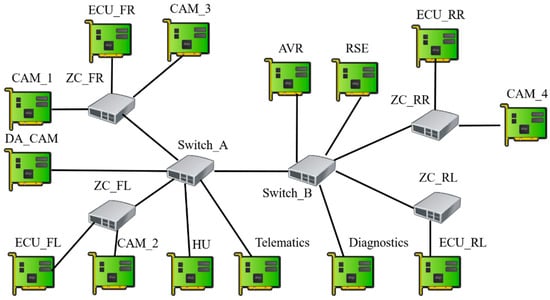
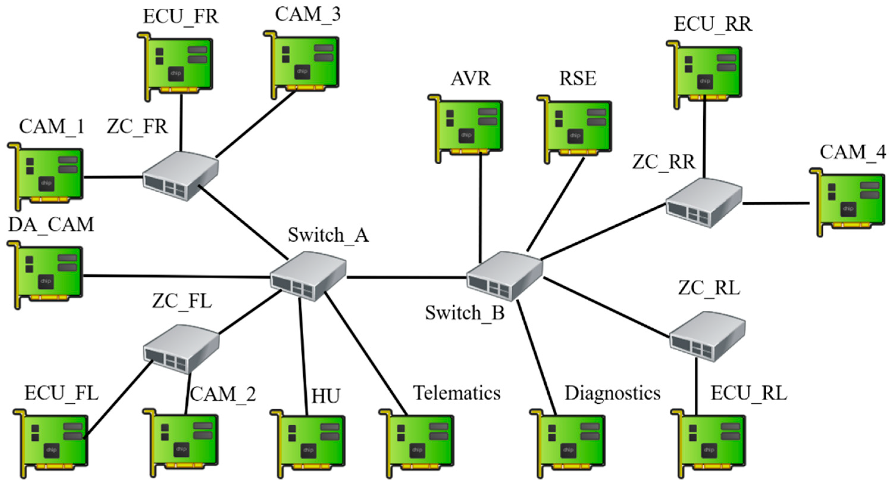
In this chapter, the accuracy of the proposed CQF schedulability analysis is verified by comparing the theoretical calculation results derived from the analytical formula with the maximum latency values obtained from simulations. Furthermore, the optimization performance and practical application value of the proposed joint scheduling mechanism are comprehensively validated via comparative experiments. Specifically, the traffic latency performance of the proposed scheduling scheme is compared with that of the traditional SP scheduling strategy under two distinct simulation scenarios, including a ring scenario and an automotive star topology scenario proposed in Ref. [24]. The analytical calculations of CPA are implemented based on the pyCPA framework [25], and all simulation experiments are conducted on the OMNeT++ platform.

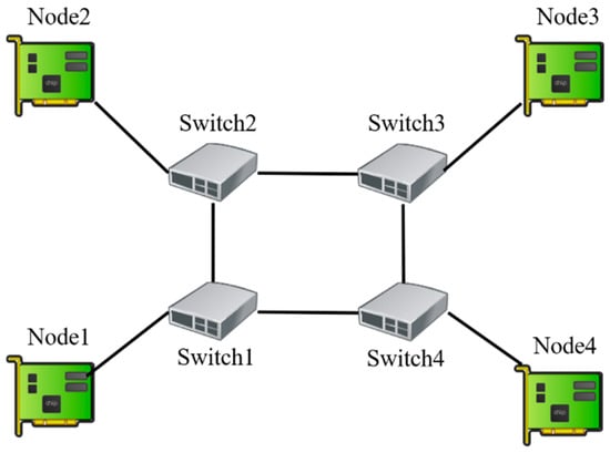
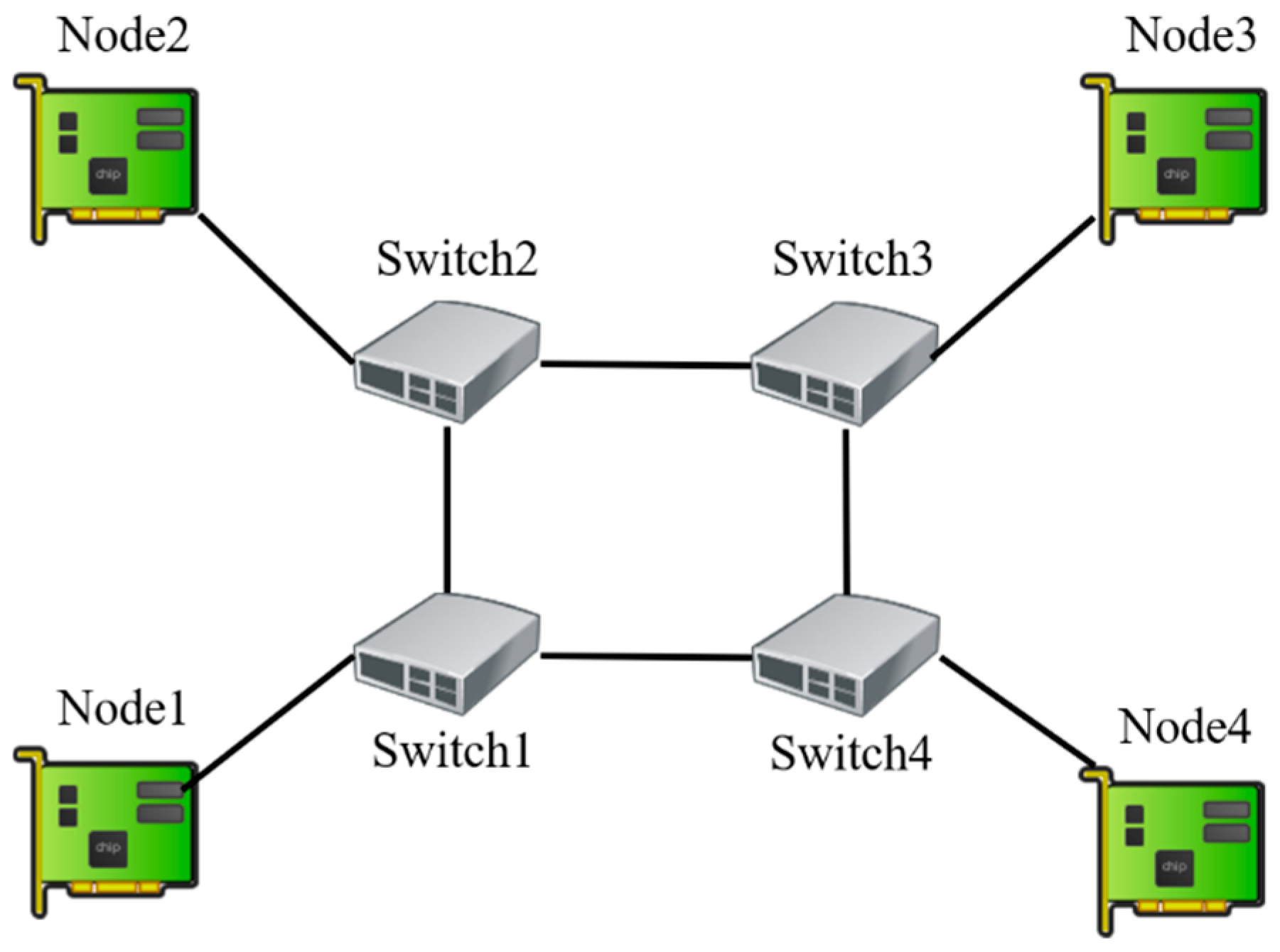
As shown in Figure 8, the schedulability calculation and simulation for the ring topology consist of four switches (Switch 1 to Switch 4) and four end nodes (Node 1 to Node 4). The data rate of all links is set to 1 Gbps. The traffic parameters in the ring scenario are presented in

Table 2. Traffic and routing table in ring scenario.

Stream Name	Priority	Period (ms)	Payload/Bytes	Source	Destination	Direction
Control1	7	100	100	Node 1	Node 2	clockwise
Video1	6	50	500,000	Node 3	Node 4	anticlockwise
Lidar1	6	100	800,000	Node 2	Node 4	clockwise
Control2	5	500	200	Node 2	Node 4	clockwise
Management1	4	500	500	Node 4	Node 2	anticlockwise
Body1	3	1000	100	Node 1	Node 3	clockwise
Audio1	2	20	300	Node 3	Node 1	anticlockwise
BE1	1	300	1000	Node 2	Node 1	anticlockwise
BE2	0	500	1400	Node 4	Node 2	clockwise

. Payload refers to the data segment of the frame. The maximum payload size of an Ethernet frame is 1500 bytes in simulation. When combined with the Ethernet header, VLAN tags, and frame check sequence (FCS), the maximum total frame length reaches 1522 bytes. Streams with payloads larger than 1500 bytes shall be segmented into multiple frames and transmitted in bursts.

The automotive star topology scenario adopted in this paper is illustrated in Figure 9, which consists of 14 network nodes and 6 switches. The configuration details of the original 37 streams are presented as Table 1 in Ref. [24]. Four new streams, namely Stream 38 to Stream 41, are added to the network. The detailed parameters of the newly added streams are listed in

Table 3. Parameters of newly added streams in the automotive star topology scenario.

Stream ID	Priority	Period (ms)	Payload/Bytes	Source	Destination
38	5	100	800	ECU_FR	DA_CAM
39	5	100	800	ECU_FL	DA_CAM
40	5	100	800	ECU_RR	DA_CAM
41	5	100	800	ECU_RL	DA_CAM

. The complete traffic and routing table are provided in Supplementary Materials Table S1. These four streams partially share transmission paths with camera streams. Furthermore, considering that the load of the camera traffic in the original scenario is too low to fully reflect the transmission characteristics of the Gigabit link, the camera traffic load is increased to ten times the original load in the Gigabit link simulation environment in this paper.

The TSN parameter settings are as follows: the TAS gating cycle is set to 500 μs, with a gating open time of 80 μs for priority 7 within a single cycle; the idleSlope parameter of the CBS mechanism within the network is set to 800 Mbps; the CQF cycle value for priorities 4 and 5 is set to 1500 us, and the CQF cycle for priorities 2 and 3 is set to 6000 μs.

3.1. CQF Schedulability Analysis Verification

To verify the accuracy of the proposed CQF schedulability analysis, it is necessary to verify whether the worst-case latency value in the simulation scenario is within the upper limit of the theoretically calculated latency. The simulation environment was run multiple times, with the random number seed reset each time, to cover as many corner cases as possible. Specifically, 50 independent simulation runs were performed for the ring scenario, with each run lasting 200 s, while another 50 simulation trials were implemented for the automotive scenario at a single-run duration of 100 s.

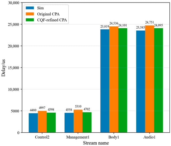
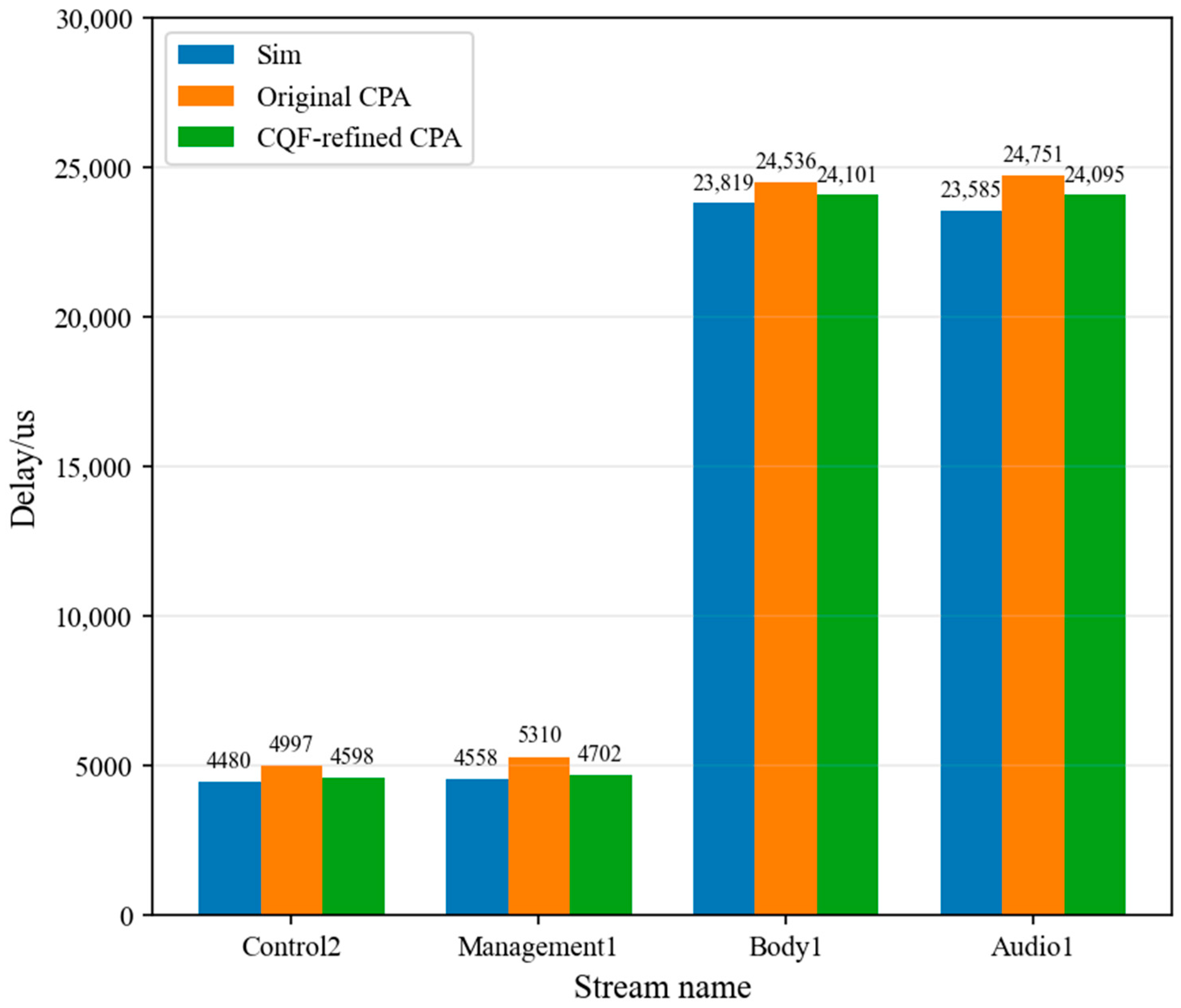
In the ring scenario, the simulation maximum latency and CPA-calculated maximum result for CQF streams are presented in

Table 4. Simulated maximum latency and calculated CPA result before and after optimization in the ring scenario.

Stream Name	Simulation Maximum Latency (μs)	Original CPA Result (μs)	CQF-Refined CPA Result (μs)	Conservative Error in Percentage (%)
Control2	4480	4997	4598	2.57
Management1	4558	5310	4702	3.07
Body1	23,819	24,536	24,101	1.17
Audio1	23,585	24,751	24,095	2.11

and Figure 10. The maximum latency simulation values for all streams in the network are less than the CPA-calculated result (both before and after optimization), which verifies the correctness of the theoretical calculations.

In this paper, the conservative error is calculated as the difference between the maximum simulation value and the CPA calculated value divided by the CPA calculated value. After optimization, the conservative errors between the calculated results and the maximum simulation latency of the four CQF streams declined to varying degrees. The original errors of 10.34%, 14.16%, 2.92% and 4.71% were reduced to 2.57%, 3.07%, 1.17%, and 2.11%, with a decrease of 7.78%, 11.09%, 1.75%, and 2.59%, respectively, showing differentiated improvement effects.

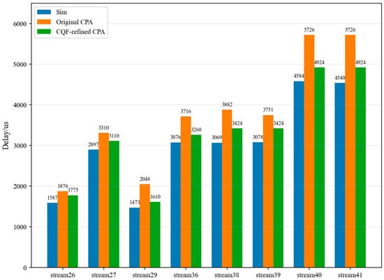
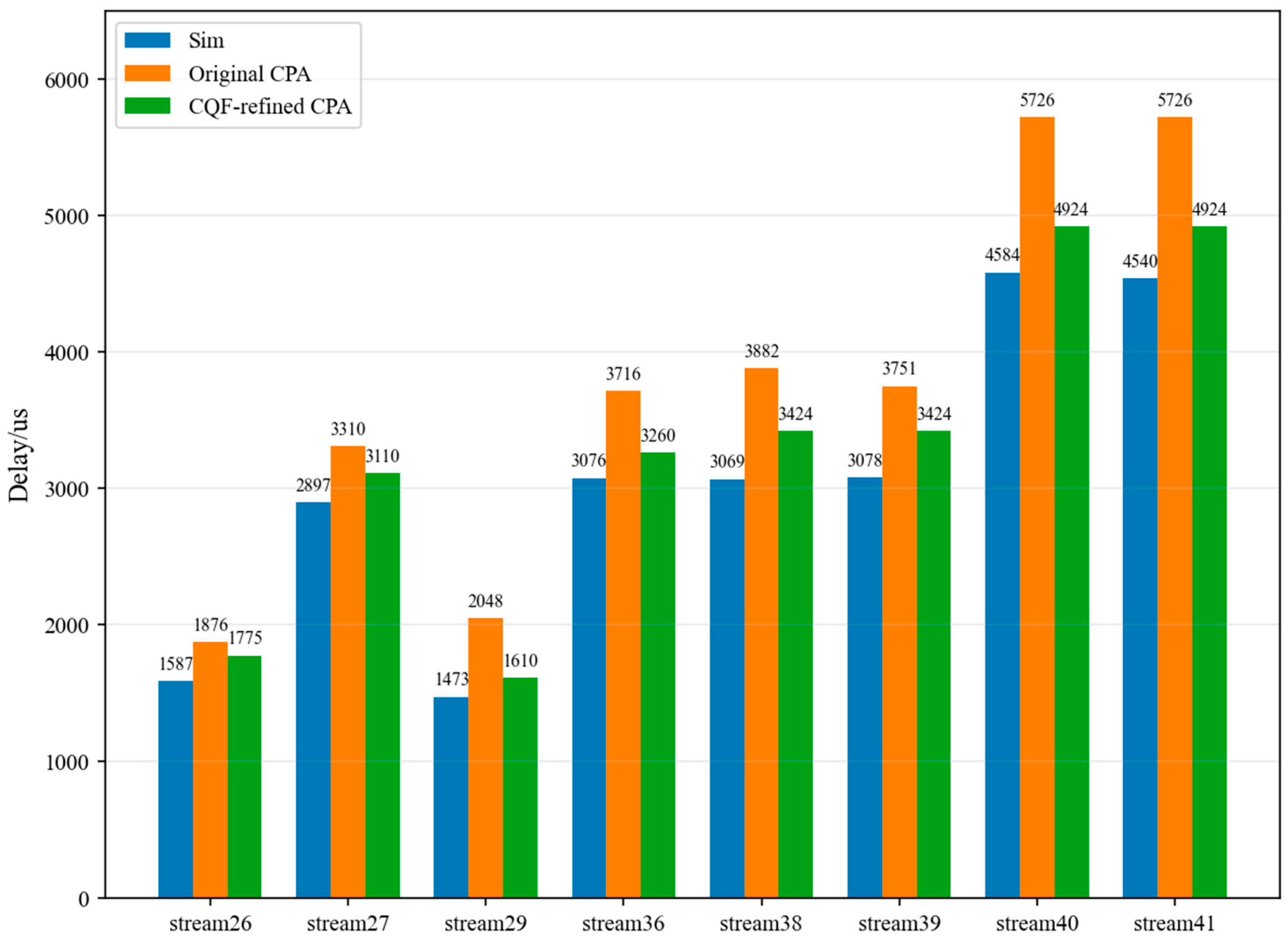
In the automotive scenario, the comparison between the simulated maximum values of CQF streams and the upper bounds calculated via CPA is presented in

Table 5. Simulated maximum latency and calculated CPA result before and after optimization in automotive scenario.

Stream ID	Simulation Maximum Latency (μs)	CPA-Calculated Result (μs)	CPA-Calculated Result After Optimizing (μs)	Conservative Error in Percentage (%)
26	1587	1876	1775	10.59
27	2897	3310	3110	6.85
29	1473	2048	1610	8.51
36	3076	3716	3260	5.64
38	3069	3882	3424	10.37
39	3078	3751	3424	10.11
40	4584	5726	4924	6.90
41	4540	5726	4924	7.80

and Figure 11. A total of eight CQF streams are configured in the simulation, and maximum latency simulation values for all CQF streams under the vehicle-mounted topology are less than the CPA-calculated results both before and after optimization. Benefiting from the optimization of the CPA analytical procedure for the CQF mechanism, the conservative errors are reduced to varying degrees. After optimization, the maximum relative error between CPA computational results and simulation measurements reaches 10.59%, while the minimum relative error is 5.64%.

3.2. Mechanism Combination Verification

To verify the effectiveness of the proposed mechanism combination, simulation results of SP, standalone TAMCQF and TAMCQF + CBS are compared in both ring and automotive scenarios.

The comparison results of delay jitter and maximum latency for traffic in the ring topology are presented in

Table 6. Simulated latency jitter and maximum latency in the ring scenario under SP, TAMCQF, and TAMCQF + CBS.

Stream Name	Jitter Under SP (μs)	Max. Latency Under SP (μs)	Jitter Under TAMCQF (μs)	Max. Latency Under TAMCQF (μs)	Jitter Under TAMCQF + CBS (μs)	Max. Latency Under TAMCQF + CBS (μs)
Control1	26	30	15	19	15	19
Video1	4243	8512	7831	13,522	4222	12,812
Lidar1	4265	11,075	7060	18,878	4139	17,684
Control2	10,202	10,211	11,416	14,402	1383	4480
Management1	3847	3856	4741	8072	1475	4558
Body1	6196	6202	8832	23,838	6263	23,819
Audio1	4243	4255	9645	21,744	7998	24,085

.

The simulated maximum value and jitter of TAS traffic are both extremely low, meeting the stringent requirements for control traffic.

The maximum latencies of the second-highest priority traffic, Video1 and Lidar1, increased from 8512 μs and 11,075 μs to 12,812 μs and 17,684 μs, respectively, after using the CBS mechanism. The increase in the maximum latency of CBS traffic is expected, as the CBS mechanism limits its bursting and prevents medium-priority traffic from experiencing excessive blocking. Video1 transmits 500,000 Bytes of data at a time, with a hop count of 5. And Lidar1 transmits 800,000 Bytes of data at a time, with a hop count of 4. The degree of latency increase is completely acceptable, and there is no significant increase in latency jitter.

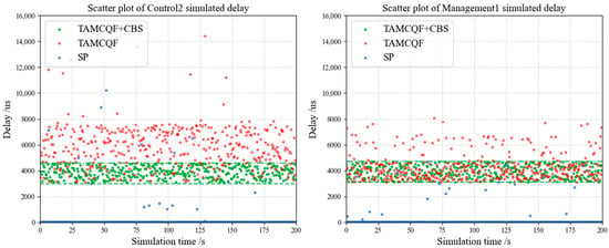
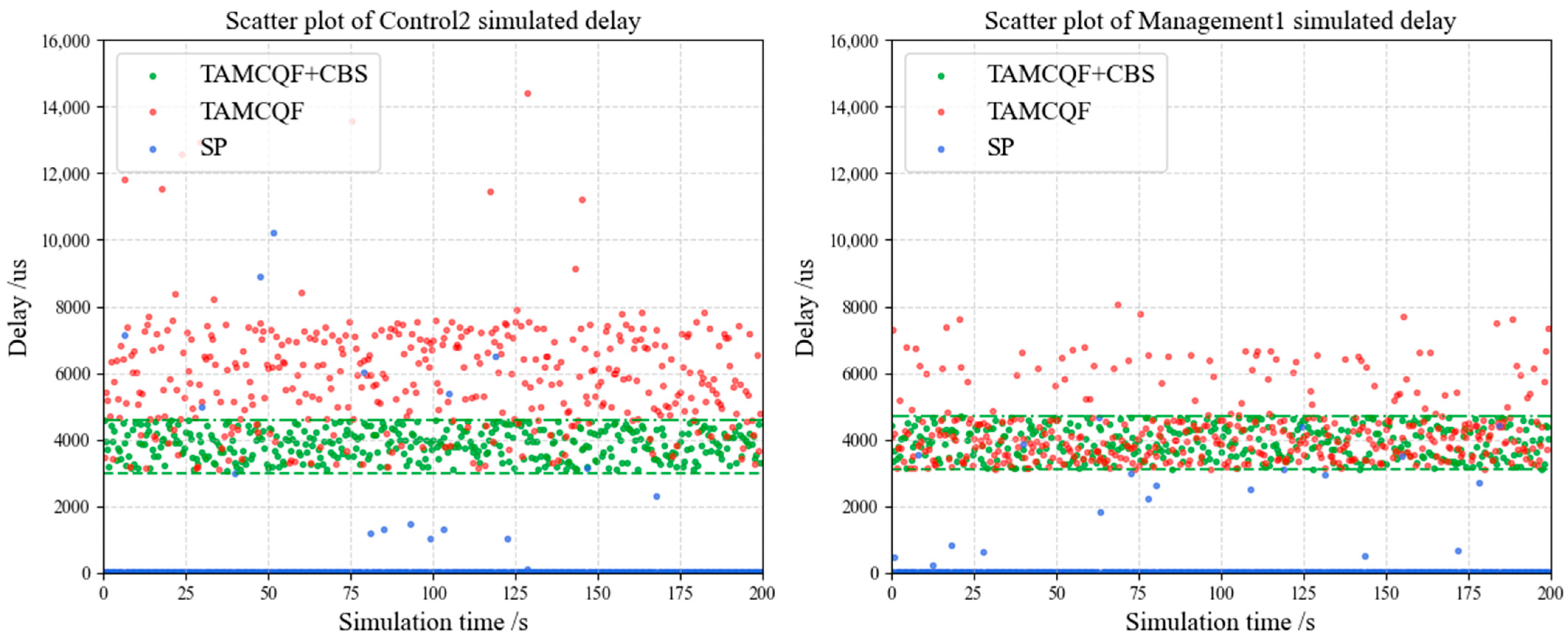
Taking the Management1 and Control2 under CQF scheduling as examples, the end-to-end latency distributions under SP policy, the deployed TAMCQF combination, and the proposed TAMCQF + CBS hybrid mechanism in this paper are illustrated in Figure 12. Under SP, the maximum latency of Control2 and Management1 reaches 10,211 μs and 3856 μs, respectively, accompanied by severe latency jitter, as indicated by the blue scatter points in the two subplots of Figure 12. This phenomenon stems from the fact that bursty high-priority streams such as Lidar1 and Video1 may occupy transmission continuously, which severely blocks the transmission of Management1 and Control2 and thereby results in a substantial gap between the maximum and minimum latency. Control2 overlaps with both Lidar1 and Video1 in transmission paths, while Management1 overlaps only with Video1. This results in a larger maximum end-to-end latency for Control2 than Management1 under the worst case. A similar issue exists for the standalone TAMCQF. Owing to the bursty and high-volume characteristics of Video1 and Lidar1 traffic, Equation (2) cannot be satisfied at several egress ports, which prevents CQF streams from acquiring stable latency guarantees. After enabling the TAMCQF + CBS, CBS effectively disperses bursty traffic, while the cyclic forwarding characteristic of the CQF mechanism constrains the upper and lower bounds of transmission latency across switches. The overall latency is confined within the range marked by the green lines in Figure 12. Compared with SP and TAMCQF, significant improvements are achieved in both latency jitter and maximum latency. For Body1 and Audio1 streams, despite an increase in latency jitter and maximum latency after mechanism deployment, CQF limits their latency jitter within two CQF cycles and restricts the maximum latency within (h + 1) × CQF cycles, where h denotes the number of network hops. Such bounded and deterministic latency performance satisfies the timing requirements of time-sensitive in-vehicle networks, which is fully acceptable for vehicular communication scenarios.

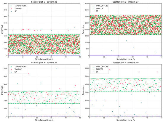
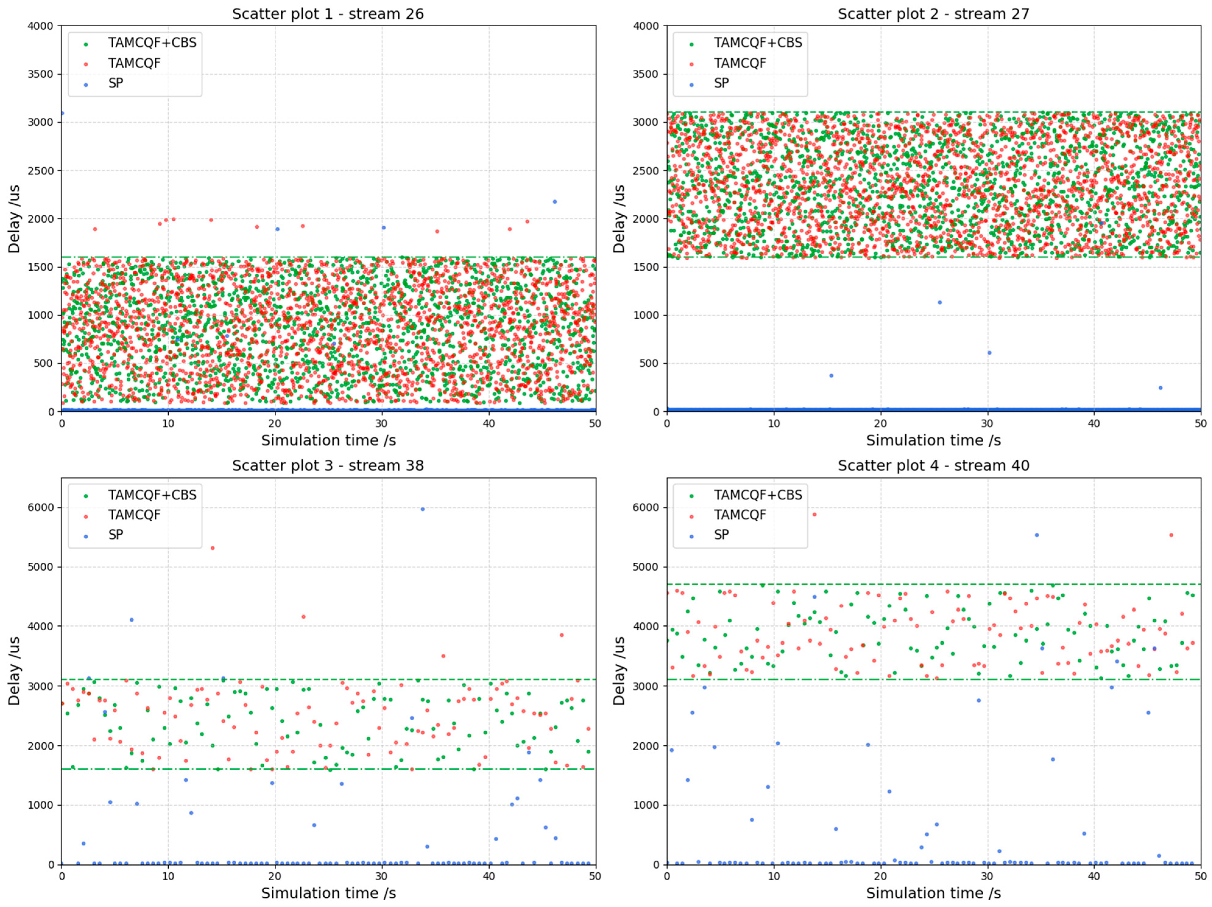
Comparisons of end-to-end latency across three scheduling mechanisms for several representative CQF streams (Stream 26, 27, 38, 40) under automotive topology are shown in

Table 7. Simulated latency jitter and maximum latency in the automotive scenario under SP, TAMCQF, and TAMCQF + CBS.

Stream ID	Jitter Under SP (μs)	Max. Latency Under SP (μs)	Jitter Under TAMCQF (μs)	Max. Latency Under TAMCQF (μs)	Jitter Under TAMCQF + CBS (μs)	Max. Latency Under TAMCQF + CBS (μs)
26	3084	3091	1909	1995	1510	1599
27	1939	1954	1599	3091	1506	3100
38	5966	5986	3717	5317	1499	3093
40	5511	5538	2753	5887	1557	4691

and Figure 13, and the derived conclusions are consistent with those obtained from the ring scenario. When CQF streams share routing paths with bursty traffic, the adoption of CBS ensures that medium-priority CQF arriving in the current CQF interval are transmitted within the subsequent interval, which improves the deterministic transmission of CQF streams. As shown in the four subplots of Figure 13, when the TAMCQF + CBS mechanism is adopted, the end-to-end delays of target traffic among the four types of traffic all fall within the range marked by the green dashed line, which matches the theoretical expectation of the CQF mechanism. Since Stream 27 has no overlapping links with bursty traffic aggregation paths, CBS deployment exerts no influence on its delay. As illustrated in subplot 2 of Figure 13, there is no obvious difference in the distribution of delay scatter points between the standalone TAMCQF mechanism and the combined TAMCQF + CBS mechanism. Stream 26 only overlaps with one bursty stream, and the optimization effect of CBS is limited. However, the maximum delay and jitter of this stream are still higher under SP and TAMCQF than TAMCQF + CBS. It can be observed from the maximum delay and jitter values of Stream 26 in Table 7, as well as the distribution of red and blue scatter points in subplot 1 of Figure 13. Furthermore, Stream 38 and Stream 40 share paths with multiple bursty streams, and the proposed TAMCQF + CBS combination yields a remarkable reduction in their maximum latency and jitter compared with SP and standalone TAMCQF, as shown in Table 7 and Subplot 4 of Figure 13.

The performance and design characteristics of each scheduling mechanism are compared in

Table 8. Comparison of different scheduling strategies.

	SP	TAMCQF	TAMCQF + CBS
Parameter design difficulty	Simple	Complex	Complex
Shaping of burst large-volume data	Not considered	Not considered	Shaped and dispersed by CBS
Latency control performance	None	Good	Good

. The SP mechanism features the simplest parameter design, while it fails to consider the shaping of burst large-volume data and has no latency control capability. The TAMCQF mechanism presents relatively complex parameter design and achieves satisfactory latency control, but it still does not support the shaping of burst traffic. By contrast, the combined TAMCQF + CBS scheme maintains the same high complexity in parameter design. On the premise of retaining excellent latency control performance, it can shape and disperse burst large-volume traffic through the CBS module, which effectively compensates for the deficiency of the single TAMCQF mechanism in handling burst traffic.

4. Conclusions

This paper proposes a combination of TSN traffic scheduling and shaping mechanisms for in-vehicle scenarios. Based on the TAMCQF model, this scheme incorporates the CBS mechanism to effectively constrain the burst traffic from periodic sensors in the autonomous driving domain, alleviating long-duration blocking of medium-priority traffic. This paper employs the CPA method to derive the upper bound of stream latency. To address the conservative error issue in CQF stream analysis under multi-hop transmission scenarios, the schedulability analysis process is optimized to obtain a more accurate expression. Simulation experiment results verify the effectiveness and accuracy of this schedulability analysis. This paper also compares the latency performance of the proposed mechanism combination with that of SP scheduling strategies. Experimental results show that the proposed mechanism can control the maximum latency of the stream, suppress latency jitter, and exhibit superior overall timing guarantee capability.

However, when multiple TSN mechanisms are combined, interactions exist between diverse mechanisms and various streams, making the parameter configuration of each mechanism a critical challenge. Therefore, future research will focus on determining optimal mechanism parameters under specific network topologies, traffic scenarios, and transmission requirements.

References

- Pei, J.; Hu, Y.; Tian, L.; Li, M.; Li, Z. A Hybrid Traffic Scheduling Strategy for Time-Sensitive Networking. Electronics 2022, 11, 3762. [Google Scholar] [CrossRef] [Scilit]
- Multiple Cyclic Queuing and Forwarding. Available online: https://www.ieee802.org/1/files/public/docs2021/new-finn-multiple-CQF-0921-v02.pdf (accessed on 26 April 2026).
- Alexandris, K.; Pop, P.; Wang, T. Configuration and Evaluation of Multi-CQF Shapers in IEEE 802.1 Time-Sensitive Networking (TSN). IEEE Access 2022, 10, 109068–109081. [Google Scholar] [CrossRef] [Scilit]
- Nie, H.; Li, S.; Liu, Y. TAMCQF: Hybrid Traffic Scheduling Mechanism Integrating TAS and Multi-CQF in TSN. In Proceedings of the 2023 IEEE Symposium on Computers and Communications (ISCC), Gammarth, Tunisia, 9–12 July 2023. [Google Scholar] [CrossRef] [Scilit]
- Nie, H.; Su, Y.; Zhao, W.; Mu, J. Hybrid Traffic Scheduling in Time-Sensitive Networking for the Support of Automotive Applications. IET Commun. 2024, 18, 111–128. [Google Scholar] [CrossRef] [Scilit]
- Deng, L.; Xie, G.; Liu, H.; Han, Y.; Li, R.; Li, K. A Survey of Real-Time Ethernet Modeling and Design Methodologies: From AVB to TSN. ACM Comput. Surv. 2022, 55, 31. [Google Scholar] [CrossRef] [Scilit]
- Diemer, J.; Thiele, D.; Ernst, R. Formal Worst-Case Timing Analysis of Ethernet Topologies with Strict-Priority and AVB Switching. In Proceedings of the 7th IEEE International Symposium on Industrial Embedded Systems (SIES), Karlsruhe, Germany, 20–22 June 2012; pp. 1–10. [Google Scholar] [CrossRef] [Scilit]
- Bordoloi, U.D.; Aminifar, A.; Eles, P.; Peng, Z. Schedulability Analysis of Ethernet AVB Switches. In Proceedings of the 2014 IEEE 20th International Conference on Embedded and Real-Time Computing Systems and Applications, Chongqing, China, 20–22 August 2014; pp. 1–10. [Google Scholar] [CrossRef] [Scilit]
- Cao, J.; Cuijpers, P.J.L.; Bril, R.J.; Lukkien, J.J. Tight Worst-Case Response-Time Analysis for Ethernet AVB Using Eligible Intervals. In Proceedings of the 2016 IEEE World Conference on Factory Communication Systems (WFCS), Aveiro, Portugal, 3–6 May 2016; pp. 1–8. [Google Scholar] [CrossRef] [Scilit]
- Cao, J.; Cuijpers, P.J.L.; Bril, R.J.; Lukkien, J.J. Independent yet Tight WCRT Analysis for Individual Priority Classes in Ethernet AVB. In Proceedings of the 24th International Conference on Real-Time Networks and Systems, Brest, France, 19–21 October 2016; pp. 55–64. [Google Scholar] [CrossRef] [Scilit]
- Cao, J.; Cuijpers, P.J.L.; Bril, R.J.; Lukkien, J.J. Independent WCRT Analysis for Individual Priority Classes in Ethernet AVB. Real-Time Syst. 2018, 54, 861–911. [Google Scholar] [CrossRef] [Scilit]
- Thiele, D.; Ernst, R.; Diemer, J. Formal Worst-Case Timing Analysis of Ethernet TSN’s Time-Aware and Peristaltic Shapers. In Proceedings of the 2015 IEEE Vehicular Networking Conference (VNC), Kyoto, Japan, 16–18 December 2015; pp. 251–258. [Google Scholar] [CrossRef] [Scilit]
- Thiele, D.; Ernst, R. Formal Worst-Case Performance Analysis of Time-Sensitive Ethernet with Frame Preemption. In Proceedings of the 2016 IEEE 21st International Conference on Emerging Technologies and Factory Automation (ETFA), Berlin, Germany, 6–9 September 2016; pp. 1–8. [Google Scholar] [CrossRef] [Scilit]
- Luo, F.; Wang, Z.; Guo, Y.; Wu, M.; Feng, W.; Sun, Z. Research on Cyclic Queuing and Forwarding with Preemption in Time-Sensitive Networking. IEEE Embed. Syst. Lett. 2023, 16, 110–113. [Google Scholar] [CrossRef] [Scilit]
- Ojewale, M.A.; Yomsi, P.M.; Nikoli, B. Worst-Case Traversal Time Analysis of TSN with Multi-Level Preemption. J. Syst. Archit. 2021, 116, 102079. [Google Scholar] [CrossRef] [Scilit]
- Luo, F.; Zhu, L.; Wang, Z.; Gan, H.; Li, Y.; Yang, Z.; Liu, D. Schedulability Analysis of Time Aware Shaper with Preemption Supported in Time-Sensitive Networks. Comput. Netw. 2025, 269, 111424. [Google Scholar] [CrossRef] [Scilit]
- Maxim, D.; Song, Y.-Q. Delay Analysis of AVB Traffic in Time-Sensitive Networks (TSN). In Proceedings of the 25th International Conference on Real-Time Networks and Systems, Grenoble, France, 4–6 October 2017; pp. 18–27. [Google Scholar] [CrossRef] [Scilit]
- Yoshimura, A.; Ito, Y. QoS Evaluation of ATS in IEEE 802.1 TSN on In-Vehicle Ethernet by Comparing with CBS and TAS. IEICE Commun. Express 2024, 13, 355–358. [Google Scholar] [CrossRef] [Scilit]
- Hellmanns, D.; Falk, J.; Glavackij, A.; Hummen, R.; Kehrer, S.; Dürr, F. On the Performance of Stream-Based, Class-Based Time-Aware Shaping and Frame Preemption in TSN. In Proceedings of the 2020 IEEE International Conference on Industrial Technology (ICIT), Buenos Aires, Argentina, 26–28 February 2020; pp. 298–303. [Google Scholar] [CrossRef] [Scilit]
- Zhao, L.; Pop, P.; Gong, Z.; Fang, B. Improving Latency Analysis for Flexible Window-Based GCL Scheduling in TSN Networks by Integration of Consecutive Nodes Offsets. IEEE Internet Things J. 2021, 8, 5574–5584. [Google Scholar] [CrossRef] [Scilit]
- Zhao, L.; Pop, P.; Craciunas, S.S. Worst-Case Latency Analysis for IEEE 802.1Qbv Time Sensitive Networks Using Network Calculus. IEEE Access 2018, 6, 41803–41815. [Google Scholar] [CrossRef] [Scilit]
- Luo, F.; Gan, H. Timing Analysis of the TSN Time-Aware Shaper Based on Compositional Performance Analysis. Recent Adv. Electr. Electron. Eng. 2025; in press. [CrossRef] [Scilit]
- Akram, B.O.; Noordin, N.K.; Hashim, F.; Rasid, M.F.A.; Salman, M.I.; Abdulghani, A.M. Joint Scheduling and Routing Optimization for Deterministic Hybrid Traffic in Time-Sensitive Networks Using Constraint Programming. IEEE Access 2023, 11, 142764–142779. [Google Scholar] [CrossRef] [Scilit]
- Leonardi, L.; Bello, L.L.; Patti, G. Bandwidth Partitioning for Time-Sensitive Networking Flows in Automotive Communications. IEEE Commun. Lett. 2021, 25, 3258–3261. [Google Scholar] [CrossRef] [Scilit]
- Diemer, J.; Axer, P.; Ernst, R. Compositional Performance Analysis in Python with PyCPA. 2012. Available online: http://retis.sssup.it/waters2012/accepted/102_Final_paper.pdf (accessed on 26 April 2026).
Disclaimer/Publisher’s Note: The statements, opinions and data contained in all publications are solely those of the individual author(s) and contributor(s) and not of MDPI and/or the editor(s). MDPI and/or the editor(s) disclaim responsibility for any injury to people or property resulting from any ideas, methods, instructions or products referred to in the content. |
© 2026 by the authors. Licensee MDPI, Basel, Switzerland. This article is an open access article distributed under the terms and conditions of the Creative Commons Attribution (CC BY) license.