Multi-Objective Operation Point Switching Strategy Based on Fuzzy Slope

Abstract

Multi-terminal voltage-source-converter-based HVDC (VSC-MTDC) systems are increasingly used to integrate renewable energy and interconnect asynchronous AC grids, but conventional fixed-coefficient droop control cannot simultaneously limit DC-voltage deviations, reduce operating losses, and preserve converter power margins during operating-point switching. This paper hypothesizes that a rule-based fuzzy adjustment of the droop slope can provide smooth multi-objective coordination without inter-station communication. A dual Mamdani fuzzy controller is developed: one controller adjusts the weighting between loss-oriented and power-margin-oriented droop coefficients according to converter power margin, while the other introduces a voltage-deviation correction according to DC-bus voltage. The controller is implemented and verified in a five-terminal MMC-based VSC-MTDC model built in PSCAD/EMTDC, where simulation data are generated under heavy-load, light-load, and power-reference switching scenarios using specified line and converter parameters. Compared with conventional droop control, the proposed strategy improves power-margin utilization, reduces operating-point discontinuities, and raises the minimum DC voltage from 370.2 kV to 381.4 kV in the severe switching case. The results confirm that fuzzy-slope droop control can achieve smoother operating-point switching and better coordinated optimization among voltage stability, operating loss, and converter reserve margin.

1. Introduction

The global push for decarbonization is reshaping power system architectures, with inverter-dominated networks increasingly displacing conventional synchronous-machine-based grids. Among the emerging technologies, modular multilevel converter (MMC)-based HVDC schemes offer particular advantages in terms of controllable power routing and modular expandability, rendering them attractive for aggregating geographically dispersed renewable generation across extended transmission distances [1,2]. When configured as multi-terminal networks (VSC-MTDC), these systems facilitate meshed power exchange among multiple asynchronous AC areas, thereby enhancing operational resilience against contingencies [3,4].

In this paper, the term voltage-source-converter-based HVDC (VSC-HVDC) refers to an HVDC transmission system in which voltage-source converters, particularly modular multilevel converters (MMCs), are used as grid-interface converters. Compared with line-commutated-converter-based HVDC systems, VSC-HVDC systems can independently regulate active and reactive power and can support weak or passive AC networks [5]. When three or more VSC stations are interconnected through DC transmission lines or cables, the system is referred to as a VSC-based multi-terminal DC (VSC-MTDC) system [6]. Therefore, the “flexibility” discussed in this paper does not denote an informal concept, but specifically refers to the controllability of VSC stations in terms of DC-voltage regulation, active-power redistribution, and coordinated operating-point adjustment among multiple converter stations. In the remainder of this paper, “VSC-MTDC system” is used to denote the MMC-based multi-terminal DC transmission system studied herein.

DC voltage is a key operational index of VSC-MTDC systems, which directly affects system stability and power transmission efficiency. In DC grids, there exists a strong coupling relationship between the active-power distribution of each converter station and DC-voltage regulation. Conventional droop control achieves power and voltage regulation by means of fixed droop coefficients, and it has been widely applied to the coordinated control of multi-terminal systems due to its advantages of no inter-station communication and fast response [7,8]. However, the fixed droop coefficients adopted in conventional droop control not only restrict the operating flexibility of DC grids, namely the capability of converter stations to coordinate DC-voltage regulation and active-power redistribution under different operating conditions, but also make it difficult to balance multiple control objectives, such as operating loss minimization, converter station power margin maintenance, and DC voltage deviation suppression [9,10].

To address the aforementioned issues, numerous improved droop control strategies have been proposed by scholars. Existing research [11] puts forward a voltage droop control scheme with adaptive reference power. By dynamically regulating the reference power, this method can compensate the operating power losses of voltage source converters (VSCs) under droop regulation. A power margin factor is introduced in [12] to improve the balance of power distribution, yet at the cost of steady-state voltage accuracy. A DC-voltage recovery strategy is proposed in [13], which regulates the supporting power of DC grids by exploiting converter-to-converter coordination alongside frequency-adaptive droop gains, thus maintaining a balance between the frequency regulation of disturbed AC systems and the voltage stability of DC grids. A voltage regulation method based on the coordination of centralized optimal control (COC) and adaptive droop control (ADC) is put forward in [14], which enhances voltage distribution and balances the power load among different VSCs. A hybrid droop control strategy is proposed in [15]; by integrating the P/V and I/V characteristic control methods, this strategy can redistribute power under grid power fluctuations and incorporate an excessive power reduction mechanism in case of overload occurrence of the converter. An improved droop control method is presented in [16], which adopts a nonlinear blending of two droop coefficients, aiming to reduce system losses, maintain power reserve, and thus achieve multi-objective optimal operation throughout the full voltage range. Another adaptive droop scheme proposed in [17] modifies the value of steady-state DC-voltage droop gain according to the available power capacity and the deviation between the maximum allowable DC voltage and the actual DC voltage. In [18], the VSC droop gain is adjusted in proportion to the square root of frequency and DC-voltage errors, enabling the converters to respond more promptly when the frequency and DC-voltage errors exceed predefined thresholds while making them insensitive to minor DC-voltage and frequency errors; the nonlinear droop gain is adopted to enhance the potential of frequency support and DC voltage regulation. Ref. [19] proposes an adaptive method to determine the droop coefficients of MTDC converters, which effectively improves the stability margin of the AC/DC hybrid power grid. However, it neither considers the overall transient performance of the system nor the impact of DC voltage fluctuations. However, the reserve power capacity of VSC stations is not taken into account when redirecting the power of VSC stations to meet control objectives.

Most of the improved droop control methods mentioned above focus on single or dual-objective optimization, and often suffer from abrupt boundary changes during control mode switching, making it difficult to achieve smooth transitions of operating points. In contrast, fuzzy control, through the flexible design of linguistic rules and membership functions, can effectively handle the dynamic coordination and smooth switching among multiple objectives, and has shown promising application potential in adaptive droop regulation for multi-terminal DC networks [20].

In MTDC systems considering the power reserve of VSCs, fuzzy inference systems (FIS) can provide feasible solutions for adaptive droop control to achieve both frequency support and DC-voltage regulation. In this regard, Reference [21] adopts a fuzzy adaptive droop controller to realize DC-voltage regulation based on local measurements. In the AC grid connected to VSC stations, the droop gain is adaptively adjusted by considering DC-voltage deviation and measured power variations, ensuring that the controller’s response to maintain DC-voltage regulation after disturbances does not extract excessive power from the AC grid connected to the VSC, which would otherwise cause AC grid instability. Reference [22] proposes frequency support from wind farm VSCs to islanded AC microgrids based on fuzzy theory. However, this study only focuses on frequency support of wind turbines in islanded AC microgrids, where the DC-voltage regulation objective is irrelevant. Reference [23] develops a fuzzy adaptive droop strategy that achieves an effective trade-off between two mutually conflicting control actions and enhances the droop controller’s robustness to parameter variations, without requiring complex mathematical modeling in the droop control design. Using a fuzzy inference system, local measurements are employed to select DC-voltage and frequency droop gains according to the general states of DC voltage, AC frequency, and available power capacity of every VSC station.

Based on the above review, existing studies on fuzzy-inference-based adaptive droop control have provided useful ideas for DC-voltage regulation, frequency support, and power distribution in VSC-MTDC systems. However, the simultaneous coordination of DC-voltage-deviation suppression, operating-loss minimization, and converter power-margin preservation during operating-point switching still requires further investigation. Therefore, this study proposes a fuzzy-slope selection method for VSC-MTDC systems. The proposed method uses the output of the fuzzy controller as an adaptive droop coefficient so that different control objectives can be emphasized under different operating conditions. Simulation results under the considered operating-point switching scenarios show that the proposed method improves the coordination among operating loss, converter power margin, and DC-voltage deviation compared with conventional fixed-coefficient droop control.

In summary, the main contributions of the proposed fuzzy adaptive droop control scheme are described as follows:

(1)

A collaborative mechanism of dual fuzzy controllers is constructed, with independent fuzzy inference units designed for loss-power margin coordination and voltage deviation suppression respectively, which simplifies the structure of the rule base and improves the operating efficiency and engineering practicality of the controller.

(2)

A fuzzy rule base for multi-objective smooth switching is designed to support dynamic trade-offs among DC-voltage stability, operating-loss minimization, and converter power-margin preservation under operating conditions such as heavy load, light load, and power disturbance.

(3)

Membership functions are defined based on physical constraints and operating characteristics, fully considering droop control stability, voltage lower limit constraints, and converter station capacity limits, so as to avoid control objective conflicts and master station competition, and enhance system robustness.

2. Topology and Operating Principle of VSC-MTDC Systems

2.1. System Topology

A VSC-MTDC system is defined as a DC transmission network in which three or more voltage-source-converter stations are interconnected through DC lines or cables [24]. In this paper, each converter station is modeled as an MMC-based VSC station. The DC-side network provides the physical path for multi-terminal power exchange, while the converter stations provide controllable interfaces between the AC grids and the DC network. Compared with conventional two-terminal HVDC systems, VSC-MTDC systems enable multi-source power injection, multi-point power reception, and decentralized DC-voltage regulation. The operational flexibility considered in this study specifically refers to the ability of droop-controlled VSC stations to redistribute active power, regulate DC voltage, and coordinate operating-point transitions under different loading conditions.

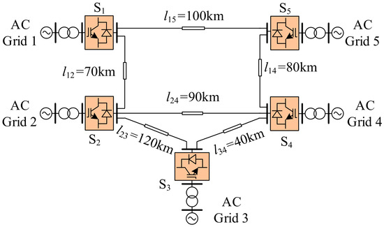
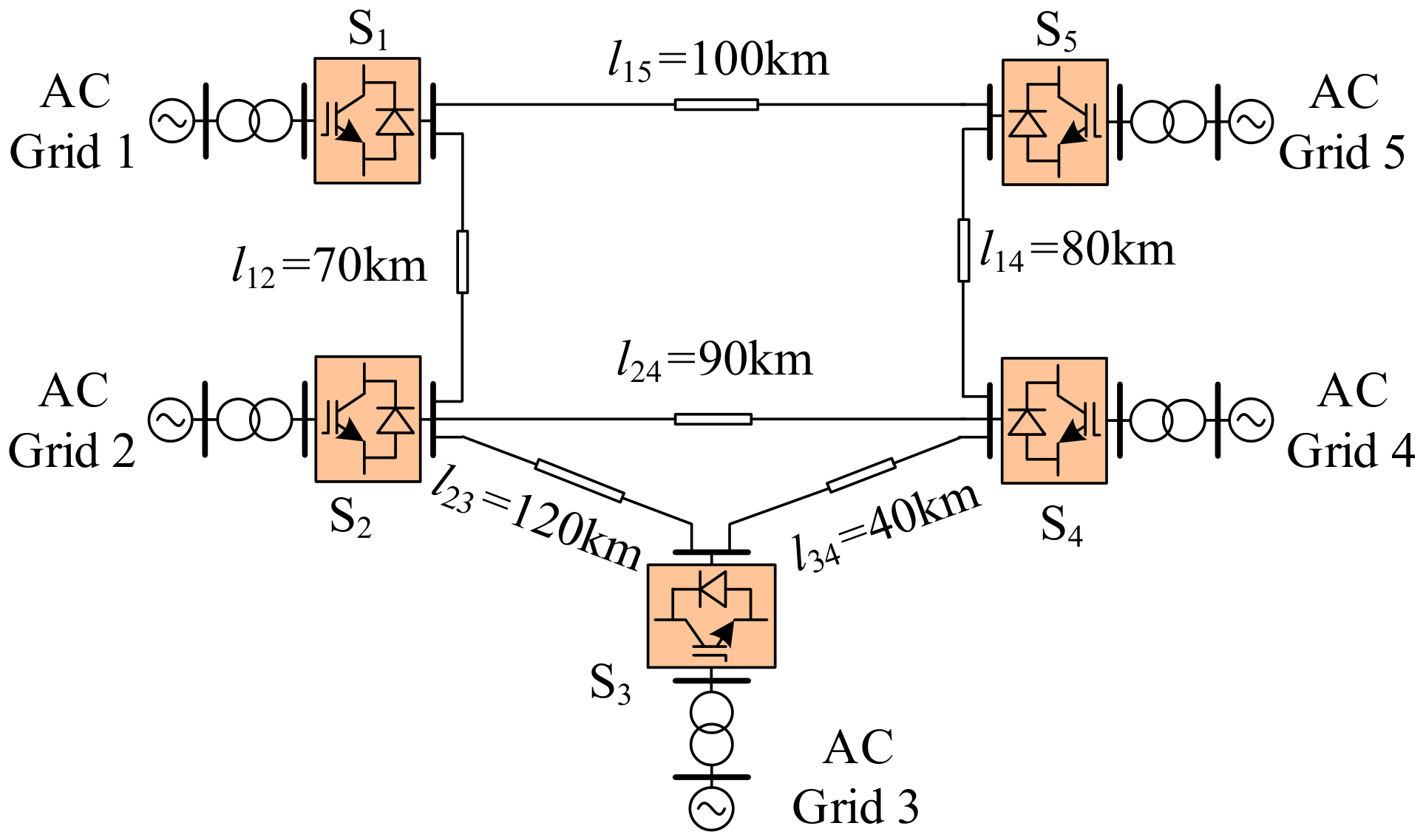
The five-terminal DC system adopted in this paper is shown in Figure 1, with converter stations numbered as S₁–S₅. The power reference direction is defined as positive when power flows from the AC system to the converter station. Converter stations S₁ and S₂ are set as rectifier stations and adopt fixed active power control. Stations S₃–S₅ operate as inverter stations and act as master stations with droop control. Their AC sides are connected to AC Grid1–AC Grid5 through converters, respectively, and the DC sides form a network via DC buses and transmission lines.

A π-type equivalent circuit is used for DC lines in this paper. The parameters of the monopolar line are set as 0.11 μF/km for capacitance, 0.1 mH/km for inductance, and 0.01 Ω/km for resistance. In the steady state, inductive components are equivalent to short circuits, capacitive components are equivalent to open circuits, and the whole line is simplified to a two-terminal resistive element.

2.2. Operating Principle

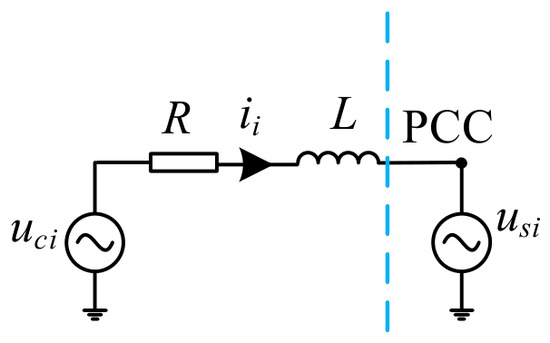
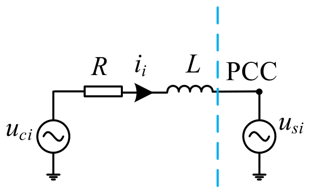
Voltage-source converters are commonly employed in VSC-HVDC converter stations, which can be modeled as an adjustable voltage source connected with an impedance, as shown in Figure 2. Here, the impedance R + jωL represents the equivalent impedance of the converter transformer and bridge arms (or the terminal impedance for two-level converters). The other end of the impedance is connected to the grid coupling point, also known as the point of common coupling (PCC). u_ci, u_si, and i_i denote the AC-side output voltage of the converter station, the PCC voltage, and the AC-side output current of the converter station for the i-th phase, respectively.

The basic structure of the equivalent circuit is independent of whether a two-level, three-level, or modular multilevel converter is adopted; the difference lies only in the calculation method of impedance parameters. All physical quantities are transformed from the abc three-phase coordinate system to the dq rotating coordinate system, with u_s assumed to be oriented along the d-axis. Neglecting the phase-locked loop (PLL) error, the mathematical model of the converter station can be expressed as:

$$\left\{\begin{array}{l}L{\displaystyle \frac{d{i}_{\mathrm{d}}}{dt}}=-R{i}_{\mathrm{d}}-\omega L{i}_{\mathrm{q}}+u_{\mathrm{c}\mathrm{d}}-u_{\mathrm{s}\mathrm{d}}\\ L{\displaystyle \frac{d{i}_{\mathrm{q}}}{dt}}=-R{i}_{\mathrm{q}}+\omega L{i}_{\mathrm{d}}+u_{\mathrm{c}\mathrm{q}}-u_{\mathrm{s}\mathrm{q}}\end{array}\right.$$

(1)

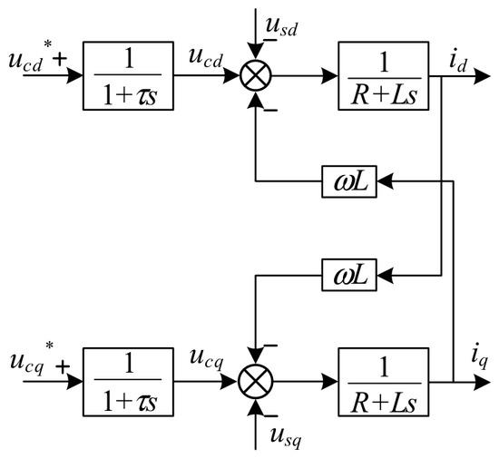
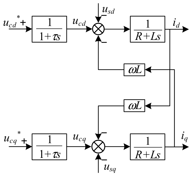
where L and R denote the equivalent inductance and resistance of the converter transformer and bridge arm, respectively; ω is the angular frequency of the AC system; i_d and i_q are the d-axis and q-axis components of the converter AC-side current, respectively; u_cd and u_cq are the d-axis and q-axis components of the converter AC-side output voltage, respectively; u_sd and u_sq are the d-axis and q-axis components of the PCC voltage, respectively. All voltage and current variables are expressed in the dq synchronous rotating reference frame. The first-order model accounts for the time delay caused by data processing and computation, as well as the switching characteristics of power electronic devices.

The relationship between the measured value and the reference value of the AC-side output voltage of the converter station is given by the equation, which is essentially an inertia link with time constant τ.

$$\left\{\begin{array}{l}{u}_{\mathrm{c}\mathrm{q}}^{\ast }=u_{\mathrm{c}\mathrm{q}}+\tau {\displaystyle \frac{d{u}_{\mathrm{c}\mathrm{q}}}{dt}}\\ u_{\mathrm{c}\mathrm{d}}^{\ast }=u_{\mathrm{c}\mathrm{d}}+\tau {\displaystyle \frac{d{u}_{\mathrm{c}\mathrm{d}}}{dt}}\end{array}\right.$$

(2)

where $u_{\mathrm{c}\mathrm{d}}^{\ast }$ and $u_{\mathrm{c}\mathrm{q}}^{\ast }$ denote the d-axis and q-axis voltage reference values generated by the converter control system, respectively.

From the above equation, the control block diagram of the model can be derived, as shown in Figure 3.

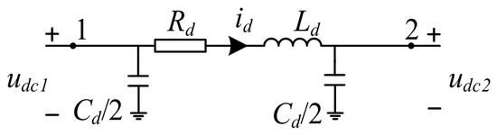
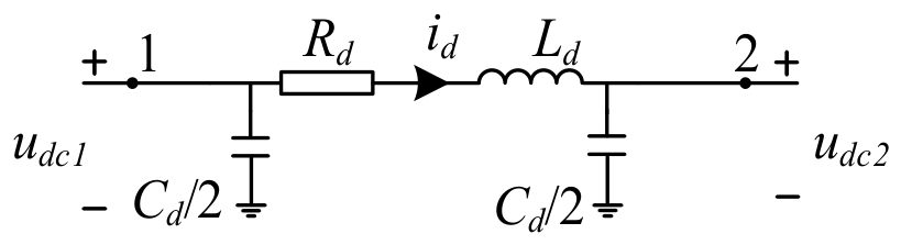
In Figure 4, R_d, L_d and C_d represent the resistance, inductance and capacitance of a single DC line respectively. u_dc1 and u_dc2 are the ground DC voltages of nodes 1 and 2, respectively. For the DC side, the DC line usually adopts the π-type equivalent modeling, which is a typical lumped parameter model, as shown in Figure 4.

Considering the influence of DC inductance, the current dynamic characteristics of the DC branch connected to the bus can be deduced as follows:

$$L_d{\displaystyle \frac{d{i}_d}{dt}}+R_d{i}_d=u_{d1}-u_{d2}$$

(3)

3. Fuzzy Droop Control Strategy

3.1. Traditional Droop Control Principle

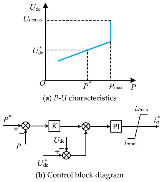
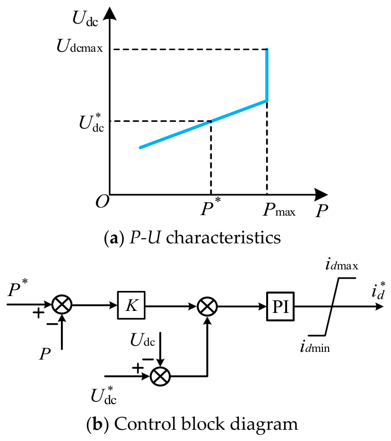
Droop-based voltage regulation in multi-terminal DC networks is a decentralized approach to DC-bus voltage management across multiple terminals. It can coordinate power sharing and DC-voltage regulation without relying on high-speed inter-station communication, which makes it suitable for systems with multiple converter stations. The core of the droop control strategy is how to select the droop slope and the controller structure, which is essentially to design and improve the P-U characteristic curve [25].

In a two-terminal VSC-HVDC system, the active-power balance can generally be maintained when one converter station operates under constant DC-voltage control. However, in a VSC-MTDC system, assigning DC-voltage regulation to only one station may reduce the utilization of converter power margins and may increase the burden on the voltage-controlling station. Therefore, several converter stations are usually operated with DC-voltage droop control, so that DC-voltage regulation and active-power redistribution can be achieved in a decentralized manner. In this context, the coordination capability of the system refers to the ability of multiple droop-controlled VSC stations to share power imbalance and regulate DC voltage without relying on high-speed inter-station communication.

In Figure 5, P and U_dc are the actual values of active power and DC voltage, respectively. P^* and $U_{dc}^{\ast }$ are the reference values of active power and DC voltage respectively. K is the droop coefficient; i_dmax and i_dmin are the upper and lower limits of the active current component respectively; u_dcmax is the upper limit of DC voltage; P_max is the maximum capacity of the converter station.

For converters operating under droop characteristics, when the DC-bus voltage changes, the transmission power value will also change.

$$P=P^{\ast }+{\displaystyle \frac{U_{\mathrm{d}\mathrm{c}}-U_{\mathrm{dc}}^{\ast }}{K}}$$

(4)

In the working process of the droop controller, the composite reference value is tracked, and the DC voltage and active power components are included. Different droop coefficients correspond to different slopes of the P-U characteristic curve, so that the control performance is balanced between power distribution and voltage deviation.

Assuming that there is no converter station controlled by DC voltage in the DC network, ignoring the loss, it is considered that the voltage of each DC node is equal. In VSC-MTDC, considering a total of n converter stations, m of which adopt droop control, when the unbalanced power ΔP occurs in the DC network, let the i-th converter station bear the unbalanced power ΔP_i; the unbalanced power ΔP of the DC network can be expressed as:

$$\Delta P={\displaystyle {\displaystyle \sum _{i=1}^m}\Delta P_i}=\Delta U_{\mathrm{d}\mathrm{c}}{\displaystyle {\displaystyle \sum _{i=1}^m}\frac{1}{K_i}}=\Delta P_j{K}_j{\displaystyle {\displaystyle \sum _{i=1}^m}\frac{1}{K_i}}$$

(5)

where ΔP_i is the unbalanced active power of the i-th converter station; K_i and K_j are the droop coefficient of the i-th and j-th droop-controlled converter station; and m is the number of converter stations operating under droop control. For the j-th converter station, the unbalanced power it bears is:

$$\Delta P_j={\displaystyle \frac{\Delta P}{K_j{\displaystyle \sum _{i=1}^m\frac{1}{K_i}}}}$$

(6)

According to the formula analysis, under DC system power imbalance conditions, the power sharing of each droop-regulated station is inversely proportional to the adopted droop coefficient. Hence, the classic droop coefficient configuration follows an inverse relationship with converter station capacity, as formulated below:

$$\forall i\ne j,K_j{P}_{\max j}=K_i{P}_{\max i}$$

(7)

where P_maxi and P_maxj are the rated active-power capacities of the i-th and j-th converter stations, respectively, This relationship indicates that conventional droop coefficients are configured according to converter capacities so that converter stations with larger rated capacities undertake a larger portion of the unbalanced power.

3.2. Fuzzy Control Principle

In the traditional control theory, the construction of the control system depends on the clear mathematical model of the controlled object. It is necessary that the control object and the disturbance can be described by strict mathematical equations, and often have clear control objectives and have the characteristics of binary logic.

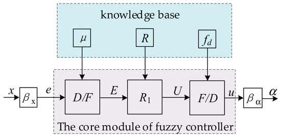
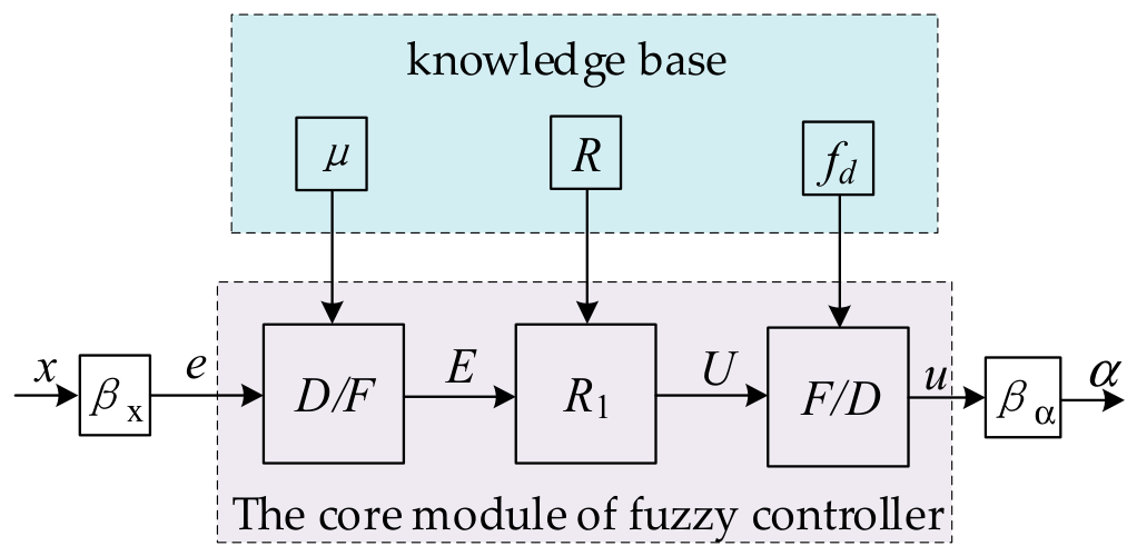
Fuzzy control is an important branch of intelligent control. Its basic control principle is to transform the control strategy described by human natural language into a fuzzy control system that can be applied to complex industrial control tasks through fuzzy sets and fuzzy logic. The fuzzy control system is mainly divided into the Mamdani type and T-S (Takagi–Sugeno) type according to whether it needs to clarify the process. In this paper, the Mamdani fuzzy control principle is used to design the controller. The basic structure of the Mamdani fuzzy controller is illustrated in Figure 6.

In Figure 6, μ is the membership function library, which stores the membership function used to transform the clear quantity into the fuzzy quantity; R is a fuzzy rule base, which stores the fuzzy conditional statements and fuzzy algorithms used in approximate reasoning. f_d is a clear method library, which stores the algorithm used to defuzzify the output fuzzy control quantity. The D/F module realizes the conversion from clear quantity to fuzzy quantity. The R₁ module realizes the approximate reasoning process from fuzzy input to fuzzy output. The F/D module realizes the conversion from fuzzy quantity to clear quantity. e and u are the input and output vectors of the core module of the fuzzy controller, corresponding to the fuzzy domain; E and U are the fuzzy input and output corresponding to e and u, respectively. x and α are the physical input and output corresponding to e and u, respectively, corresponding to the physical domain of discourse; β_x is the quantization factor, and β_α is the scaling factor. The proportional transformation and scaling of the input and output clear variables between the clear and fuzzy domains are realized respectively. In particular, the translation of the domain is also completed by this part of the module.

Furthermore, if the dimensions of the input and output vectors are one-dimensional, the fuzzy controller is called a single-variable fuzzy controller (SISO). A fuzzy controller with multiple input and output variables is called a multivariable fuzzy controller (MIMO). The single-output fuzzy controller is often used in the actual industrial control system, and the MIMO system is often realized by the combination of multiple single-output fuzzy controllers.

3.3. DC Voltage Steady-State Deviation Characteristics of Droop Control

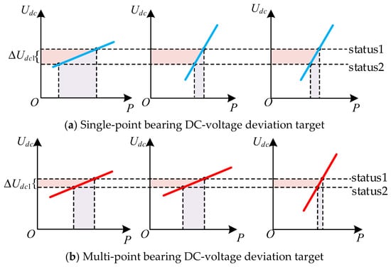
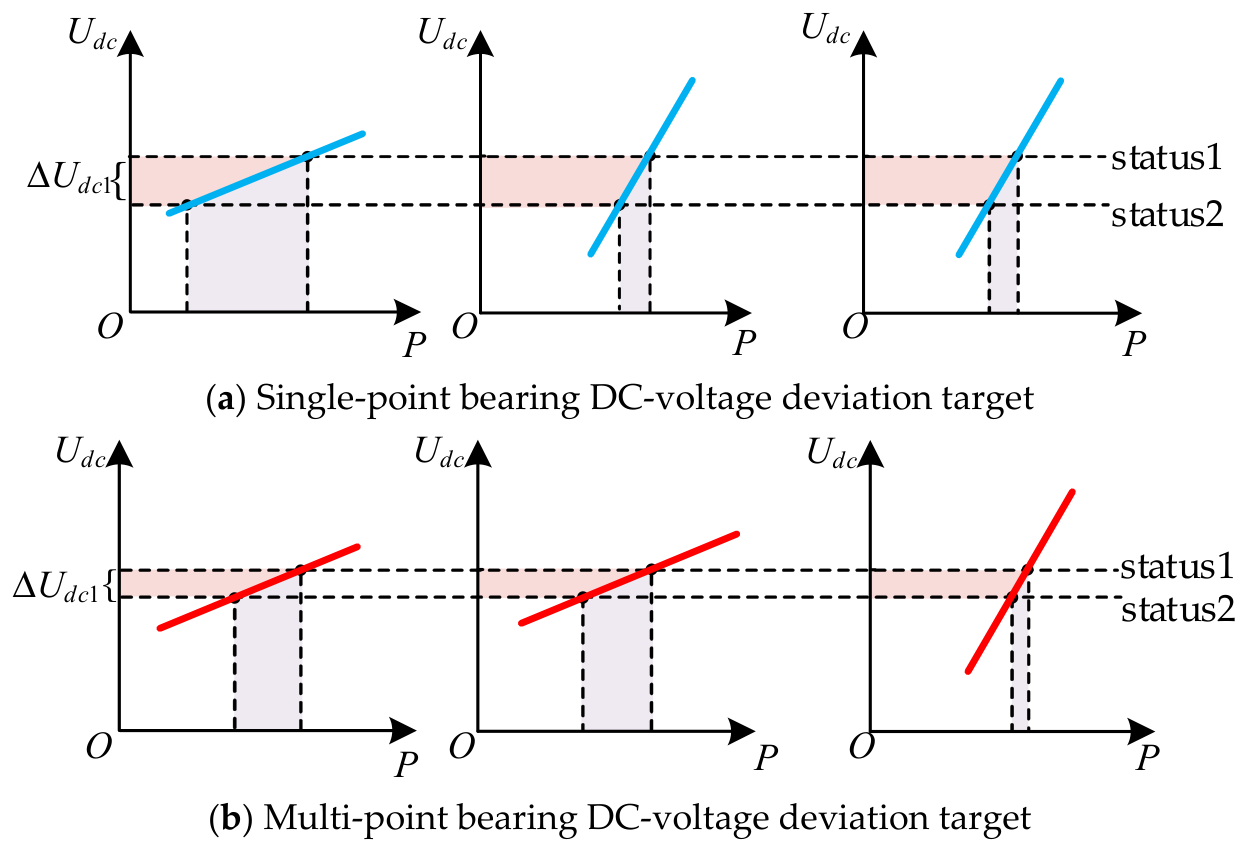
Since the droop coefficient reflects both voltage deviation and power deviation, the greater the droop coefficient—that is, the more the P-U characteristic curve tends to be horizontal—the stronger the DC-voltage rigidity, and the smaller the steady-state DC-voltage deviation. The higher the number of droop control converter stations that can achieve the above operating point switching characteristics at any time, the better the control target is achieved. As shown in Figure 7, if two droop control stations show the goal of reducing DC-voltage deviation, considering the same negative unbalanced power, the DC-voltage reduction is significantly smaller than that of a single droop control station, which is shown in the figure. When the lower limit of the slope is reasonably controlled, due to the characteristics of droop control, the phenomenon of master station contention will not occur.

3.4. The Goal Establishment of Fuzzy Control and the Switching of Operating Conditions

The steady-state operating point of the VSC-MTDC transmission system depends on the active power control strategy adopted by each converter station. The specific performance is the design and balance of the P-U characteristic curve of each converter station; that is, the power balance between the sending and receiving ends is satisfied, and the sending end DC node is equal to the receiving end node voltage after considering the line voltage drop. Considering that the converter stations on the power receiving side adopt droop regulation mode, the operating point depends on the equilibrium point of the P-U characteristic profile of each droop control station.

When the P-U characteristics of the droop control station consider a single control target design, there are often other operating intervals with poor control performance. In order to solve this problem, the P-U characteristic curve is designed by considering multiple control objectives. The segmented coordination decision results of each control target are expressed in language as follows: if the voltage of the DC bus of the converter station is small, the droop coefficient of the converter station is reduced, but the power of any converter station cannot be less than its lower power limit; if the active power of the converter station is large, the droop coefficient of the converter station is increased. If the operating point of the converter station does not belong to the above two cases, the droop coefficient of the converter station is kept at the optimized value.

In the actual control system of the converter station, a clear control logic is adopted, and the fuzzy boundaries such as large and small cannot be identified. If a clear boundary is set up by considering the idea of piecewise function, the switching between the objectives will be realized in a clear numerical value, which limits the self-organization and self-adaptation performance of the controller to a certain extent, and reduces the linearity of the controller near the boundary point. The fuzzy logic controller (FLC) is good at dealing with the multi-objective decision-making problem with unclear boundary points due to the use of fuzzy logic. Therefore, the coordinated decision-making of droop coefficient selection for different objectives of each converter station can be realized, and the smooth switching of system operating points can be realized. The introduction of fuzzy droop coefficient K^* is shown in Equation (8):

$$K^{\ast }=(1-\alpha )K_1+\alpha K_2-\beta$$

(8)

where K₁ is the droop coefficient obtained by considering the minimum optimization of operating loss; K₂ is the droop coefficient calculated by considering the power margin of the converter station; α is a fuzzy weight factor, which changes the proportion of the loss term and margin term with the change in output active power of the converter station. b is the output fuzzy variable of the fuzzy controller under light-load operating conditions; β is the fuzzy impairment coefficient. With the change in DC-bus voltage, different values are taken, corresponding to the clear result of b. Considering the two operating conditions below, the operation point switching scheme of fuzzy droop control is introduced respectively.

3.5. Generation Method of Fuzzy Slope

The FLC1 and FLC2 are described by considering two operating conditions of heavy load and light load respectively.

(1)

Heavy-load operating conditions

If the active power of the converter station gradually increases from the vicinity of the command value, in order to avoid the full load of the converter station and make the power reasonably distributed among the converter stations to improve the capacity utilization efficiency, the control target selected by the droop coefficient should gradually transit from the target of minimizing the operating loss of the DC system to the target of maintaining the power margin of the converter station. In Equation (8), the fuzzy weight factor α gradually increases from 0 to 1. On the contrary, when the active power of the converter station gradually decreases from the vicinity of the capacity, in order to reduce the operating loss, the control target selected by the droop coefficient should gradually transition from the power margin target of the converter station to the minimum operating loss target of the DC system. In Equation (8), the fuzzy weight factor α is gradually reduced from 1 to 0. Considering that there is no overload of the converter station in the transition zone, the design can reduce α from 1 to 0 as an acceleration process, and accelerate the switching to reduce the operating loss control target when the active power decreases.

The switching of the two control objectives only needs to consider the converter station’s power regulation margin. The α is selected as the fuzzy output of the fuzzy controller, and the scale factor is 1, so that the physical output is also α; (P_max − P) is used as the physical input of the fuzzy controller, corresponding to the fuzzy variable e; the quantization factor is 1/(P_max − P*), then:

$$e={\displaystyle \frac{P_{\max }-P}{P_{\max }-P^{\ast }}}$$

(9)

where e is the normalized fuzzy input of FLC1; P_max is the maximum active-power capacity of the converter station; P is the actual active power of the converter station; and P* is the active power command or reference value. The term (P_max − P) represents the remaining power regulation margin of the converter station, while (P_max − P*) is used as the normalization base. Therefore, e is a dimensionless variable used to determine whether the controller should emphasize operating-loss minimization or converter power-margin preservation.

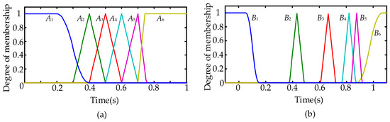
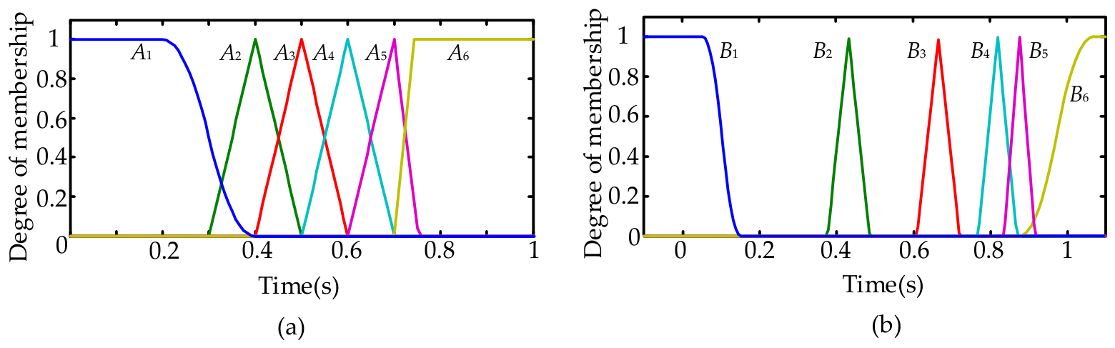
The fuzzy distribution of input and output variables is shown in Figure 8. The membership functions involved mainly consider triangular, trapezoidal, Z-type and S-type. A₁~A₆ and B₁~B₆ represent fuzzy subsets of input variables and output variables, respectively, a total of 12. Among them, A₁ and B₁ are Z-type, B₆ is S-type, A₆ is trapezoid, and the rest are triangles. The fuzzy rule table is shown in

Table 1. Fuzzy rule table.

e	A1	A2	A3	A4	A5	A6
α	B6	B5	B4	B3	B2	B1
weight	0.25	0.25	0.25	0.25	0.25	1

. The clarification algorithm is selected as the area center method (centroid).

The shapes of the membership functions are selected according to the physical meaning of different operating regions and the requirement of smooth objective switching. The Z-shaped and S-shaped membership functions are adopted at the two boundary regions because they can represent saturated fuzzy states. For example, when the converter station approaches its power limit, the power-margin preservation objective should be fully activated; when the converter station has sufficient power regulation margin, the loss-minimization objective should dominate. The triangular membership functions are used in the transition region because they provide simple and continuous overlapping intervals between adjacent fuzzy subsets, which enables approximately linear interpolation of the fuzzy output and avoids abrupt changes in the droop coefficient. The trapezoidal membership function is used in the relatively stable operating interval to maintain the controller output within a constant range and to reduce the sensitivity of the controller to small active-power fluctuations. Therefore, the adopted membership-function shapes are determined by the requirements of boundary saturation, smooth transition, and robustness against minor operating-point variations, rather than by arbitrary selection.

The fuzzy control rules in Table 1 state that in the transition region, if the active power decreases (i.e., e increases), then α decreases. As e increases, the converter station’s power regulation margin increases, and a smaller α increases the proportion of K₁ in K^*. Correspondingly, when e falls into A₁∼A₆, α belongs to B₆∼B₁. To make the decrease in α exhibit an accelerating process, the intervals of B6∼B1 are gradually widened. For example, when e increases uniformly from 0.4 to 0.6, the fuzzy set output by the fuzzy controller before defuzzification gradually transitions from being entirely B₅, at the same rate to a mixture of B₄ and B₅; then entirely B₄; further at the same rate to a mixture of B₃ and B₄; and finally entirely B₃. Although the transition speed remains constant, the contribution of each fuzzy set to the reduction in the centroid satisfies B₃ > B₄ > B₅, so that the defuzzified result shows an accelerated decrease.

Since the critical value of the fuzzy input at which the switching of control objectives is completed cannot be determined, a transition region must be set. The physical meaning of the transition region is that the transition of control objectives is accomplished within this interval. In Figure 8, it is represented as the interval between the extreme point of A₂ and that of A₅, corresponding to e ∈ [0.4, 0.7]. Outside this region, the switching of control objectives is considered to be completed. The variation in α is gentle on the left side of this region and steep on the right side; therefore, the corresponding membership functions are designed to be gentle and steep, respectively. Meanwhile, through debugging, to further enhance the steepness of α variation on the right side of the transition region, the first five fuzzy rules are set with equal weights, and the weight of the last fuzzy rule is four times that of the fourth rule. It is worth noting that if the right boundary of the transition region is m, the selection criterion for this multiple is that the steepness of α variation in the right neighborhood of m is significantly greater than that in the left neighborhood.

Meanwhile, when the fuzzy input takes the core values of A₁ and A₆ respectively, the corresponding values of α are 1 and 0. Under the centroid defuzzification algorithm, the universe of discourse of the output variable cannot be set as [0, 1]. Otherwise, the actual maximum value of α would be less than 1 and the minimum value greater than 0, making it impossible to achieve full switching of operating points corresponding to the control objectives. Through debugging, the universe of discourse of the output variable is set as [−0.1, 1.1] in this paper, while the actual range of the defuzzified result is constrained within [0, 1].

Considering the fluctuations in the converter station’s active power during transient processes, to improve the robustness of the controller, let

$$\alpha =\left\{\begin{array}{l}0e>1\\ 1e<0\\ evalfis1(e)0\le e\le 1\end{array}\right.$$

(10)

where α is the crisp output of FLC1 after defuzzification; evalfis1(e) denotes the output of the first Mamdani fuzzy inference system with e as the input; and e in [0, 1] denotes the transition region between the loss-oriented and power-margin-oriented control objectives. When e > 1, the converter station has sufficient power margin and α is set to 0, so the controller mainly selects K₁. When (e < 0), the converter station approaches or exceeds its power limit and α is set to 1, so the controller mainly selects K₂.

(2)

Light-load operating conditions

If the converter station’s DC-voltage gradually decreases from the vicinity of the command value, in order to avoid the steady-state DC-voltage being too small to trigger the related protection, the control target selected by the droop coefficient should gradually transit from the target of minimizing the operating loss of the DC system to the target of reducing the DC-voltage deviation. In Equation (8), the fuzzy impairment coefficient β increases gradually from 0. On the contrary, when the converter station’s DC voltage gradually increases from the lower limit value, in order to reduce the operating loss, the control target selected by the droop coefficient should gradually transition from the target of reducing the DC voltage deviation to the target of minimizing the operating loss of the DC system. In Formula (8), the fuzzy impairment coefficient β is gradually reduced to 0. Considering that there is no low-voltage over-limit of the converter station in the transition zone, the design can reduce β to 0 as an acceleration process, and accelerate the switching for the operating loss reduction control target when the DC voltage increases. For any droop control station, the switching of the two control objectives only needs to consider the DC voltage deviation of the converter station. (U − U_min) is selected as the physical input of the fuzzy controller, corresponding to the fuzzy variable u, and the quantization factor is 1/(U_dc^* − U_dcmin). The practical realization of the fuzzy controller, referred to as the fuzzy output b, is mathematically formulated as follows:

$$\left\{\begin{array}{l}u={\displaystyle \frac{U_{\mathrm{d}\mathrm{c}}-U_{\mathrm{d}\mathrm{c}\mathrm{m}\mathrm{i}\mathrm{n}}}{U_{\mathrm{d}\mathrm{c}}^{\ast }-U_{\mathrm{d}\mathrm{c}\mathrm{m}\mathrm{i}\mathrm{n}}}}\\ b=\gamma {\displaystyle \frac{\beta }{K_1}}\end{array}\right.$$

(11)

where u is the normalized fuzzy input of FLC2; U_dc is the actual DC-bus voltage of the converter station; U_dcmin is the lower admissible DC-voltage limit; and $U_{\mathrm{d}\mathrm{c}}^{\ast }$ is the rated or reference DC-bus voltage. b is the crisp output of FLC2 after centroid defuzzification. The term (U_dc − U_dcmin) represents the remaining DC-voltage security margin, while ($U_{\mathrm{d}\mathrm{c}}^{\ast }$ − U_dcmin) is used as the normalization base. Therefore, u is a dimensionless variable used to determine whether the controller should shift from the loss-oriented operating point to the DC-voltage-support-oriented operating point; γ is the station number validity factor.

The value of γ is determined according to the minimum admissible margin of the adaptive droop coefficient. Under low-voltage support conditions, the actual power of the converter station is lower than its command value, and the fuzzy weighting factor satisfies α = 0. Thus, the adaptive droop coefficient in (8) can be simplified as:

$$K^{\ast }=K_1-\beta$$

(12)

From Equation (11), the adaptive droop coefficient can be further expressed as:

$$K^{\ast }=K_1(1-{\displaystyle \frac{b}{\gamma }})$$

(13)

The strongest voltage-support correction occurs when b = 1, and the minimum value of the adaptive droop coefficient is therefore:

$$K_{\min }^{\ast }=K_1(1-{\displaystyle \frac{1}{\gamma }})$$

(14)

If γ = 1, then $K_{\min }^{\ast }$ = 0, which means that the droop-controlled station is equivalent to a constant DC-voltage control station. When multiple droop-controlled stations enter this state simultaneously, master-station competition may occur and the stability of the DC grid may be weakened. Therefore, a nonzero lower bound of K^* should be retained. In this paper, a 0.1 p.u. minimum droop coefficient margin is retained to avoid the above problem, namely:

$${\displaystyle \frac{K_{\min }^{\ast }}{K_1}}=1-{\displaystyle \frac{1}{\gamma }}=0.1$$

(15)

Therefore, γ = 1.11 is determined by the requirement of maintaining a nonzero adaptive droop coefficient while preserving sufficient low-voltage support capability.

The membership functions of FLC2 are designed according to the same principle as FLC1, but the physical input is changed from the converter power regulation margin to the DC-voltage security margin. The Z-shaped and S-shaped functions describe the saturated low-voltage and normal-voltage boundary regions, respectively. The triangular functions provide smooth interpolation in the voltage-transition region, while the trapezoidal function improves robustness when the DC voltage varies within a stable range. This design ensures that the voltage-support objective can be gradually activated when the DC voltage approaches its lower admissible limit, while unnecessary switching caused by small voltage fluctuations can be avoided.

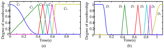
The fuzzy distributions of input and output variables are shown in Figure 9, where the involved membership functions mainly include triangular, trapezoidal, Z-shaped, and S-shaped types. C₁∼C₆ and D₁∼D₆ denote the fuzzy subsets of the input and output variables, with a total of 12 subsets.

In accordance with the fuzzy control rules of

Table 2. Fuzzy rule table.

u	C1	C2	C3	C4	C5	C6
b	D6	D5	D4	D3	D2	D1
weight	0.25	0.25	0.25	0.25	0.25	1

, within the transition region, if the DC-voltage increases (i.e., u increases), then b decreases. As u increases, the negative DC voltage deviation is reduced, and the fuzzy reduction coefficient is decreased to increase K^*. Correspondingly, when u belongs to C₁∼C₆, b belongs to D₆∼D₁. To make the decrease in b exhibit an accelerating process, the intervals of D₆∼D₁ are gradually widened. When u increases at a constant rate, the gradual change principle of fuzzy inference is the same as that of the fuzzy controller corresponding to Figure 8 and Table 1. Although the transition speed remains unchanged, the contribution of each subset to the reduction in the overall centroid satisfies B₃ > B₄ > B₅, so that the defuzzified result shows an accelerated decrease. The transition region is set as u ∈ [0.4, 0.6], and the switching of control objectives is considered to be completed outside this region.

The difference from the fuzzy controller corresponding to Figure 8, Table 1, and Equation (10) is that a station number validity factor γ is added to avoid excessively small values of K^*. In addition, considering the lower limit requirement of the droop slope and to improve the control performance for DC-voltage deviation, the selections corresponding to C₁ and C₂ on the left side of the transition region are designed to be gentler, so that the ramp smoothness of the fuzzy output variable is improved as the input variable decreases. The platform width of C₁ is reduced, thereby narrowing the bandwidth where the output variable remains at 1, which reduces the risk of master station competition among droop-controlled converter stations that undertake the objective of reducing DC-voltage deviation.

Considering the fluctuations of DC voltage during transient processes, to enhance the robustness of the controller, let

$$b=\left\{\begin{array}{l}0u>1\\ 1u<0\\ evalfis2(u)0\le u\le 1\end{array}\right.$$

(16)

where evalfis2(u) denotes the output of the second Mamdani fuzzy inference system with u as the input; and u in [0, 1] denotes the transition region between the loss-oriented and voltage-support-oriented control objectives. When u > 1, the DC voltage is sufficiently far from its lower limit and b is set to 0, so the fuzzy correction coefficient β is not activated. When u < 0, the DC voltage approaches or falls below the lower admissible limit and b is set to 1, so the controller provides the strongest DC-voltage support correction.

To further clarify the parameterization and implementation of the two fuzzy controllers, the key design information of FLC1 and FLC2 is summarized in

Table 3. Parameterization of the proposed fuzzy controllers.

Controller	Input Variable	Normalization	Output Variable	Membership Functions	Defuzzification	Function
FLC1	Pmax − P	e = (Pmax − P)/(Pmax − P*)	α	Z, triangular, trapezoidal, S	Centroid	Loss–margin coordination
FLC2	Udc − Udcmin	u = (Udc − Udcmin)/($U_{\mathrm{d}\mathrm{c}}^{\ast }$ − Udcmin)	b, β	Z, triangular, trapezoidal, S	Centroid	Voltage-support correction

.

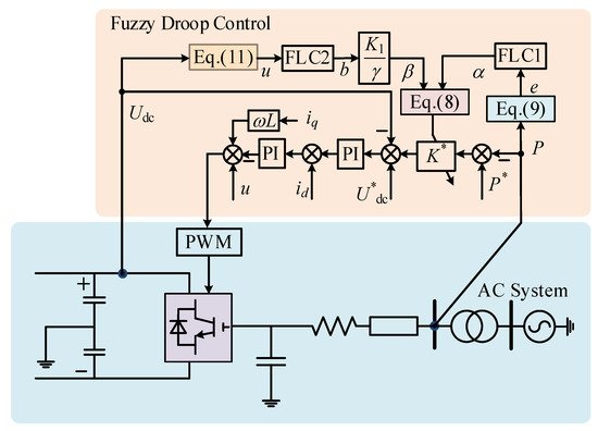
From the above analysis, the principle of the droop control for VSC-MTDC with fuzzy slope is shown in Figure 10, where u_d is the actual d-axis component of the AC-side output voltage of the converter station; i_q is the actual q-axis component of the AC-side output current of the converter station; FLC1 denotes the fuzzy controller corresponding to Figure 8, Table 1, and Equation (10); and FLC2 denotes the fuzzy controller corresponding to Figure 9, Table 2, and Equation (12).

The membership functions of both FLC1 and FLC2 are designed according to converter operating constraints and the required smoothness of operating-point switching. Z-shaped and S-shaped membership functions are used at the boundary regions to represent saturated operating states, triangular membership functions are used in the transition region to ensure continuous switching between adjacent control objectives, and trapezoidal membership functions are used to maintain the controller output within a stable operating interval. The transition regions are selected according to the converter power margin and DC-voltage security margin, rather than by arbitrary numerical partitioning. The rule weights are introduced to accelerate the recovery from power-margin-oriented or voltage-support-oriented operation to loss-oriented operation once the emergency condition disappears.

The fuzzification process converts the normalized inputs (e) and (u) into the corresponding membership degrees. The fuzzy inference process is then performed using the rule bases listed in Table 1 and Table 2. Finally, the centroid defuzzification method is adopted to obtain continuous crisp outputs α and β. The centroid method is selected because it can avoid discontinuous jumps in the droop coefficient and thus improve the smoothness of operating-point switching. The final adaptive droop coefficient K^* is calculated by substituting α, K₁, K₂, and β into (9). This coefficient is then embedded into the outer droop control loop to generate the active-power/current reference, which is subsequently tracked by the inner current controller of the converter station.

In the PSCAD/EMTDC implementation, the fuzzy controller is executed at each droop-controlled converter station using local measurements of active power and DC-bus voltage. No inter-station communication is required. At each control step, the measured actual active power and actual DC-bus voltage are normalized, fuzzified, processed through the corresponding fuzzy rule bases, defuzzified, and finally converted into the adaptive droop coefficient K^*. Therefore, the proposed strategy can be reproduced by specifying the input normalization equations, membership functions, rule bases, rule weights, defuzzification method, and droop coefficient updating equation.

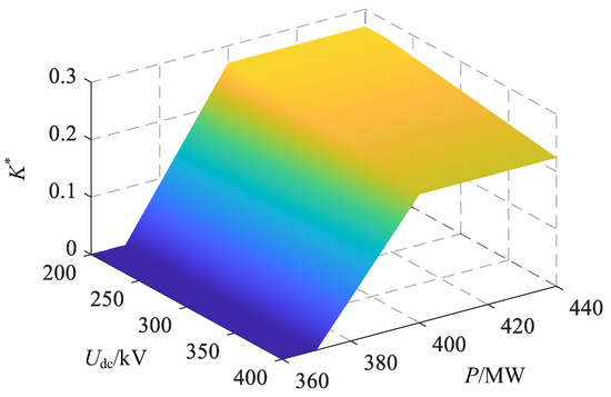
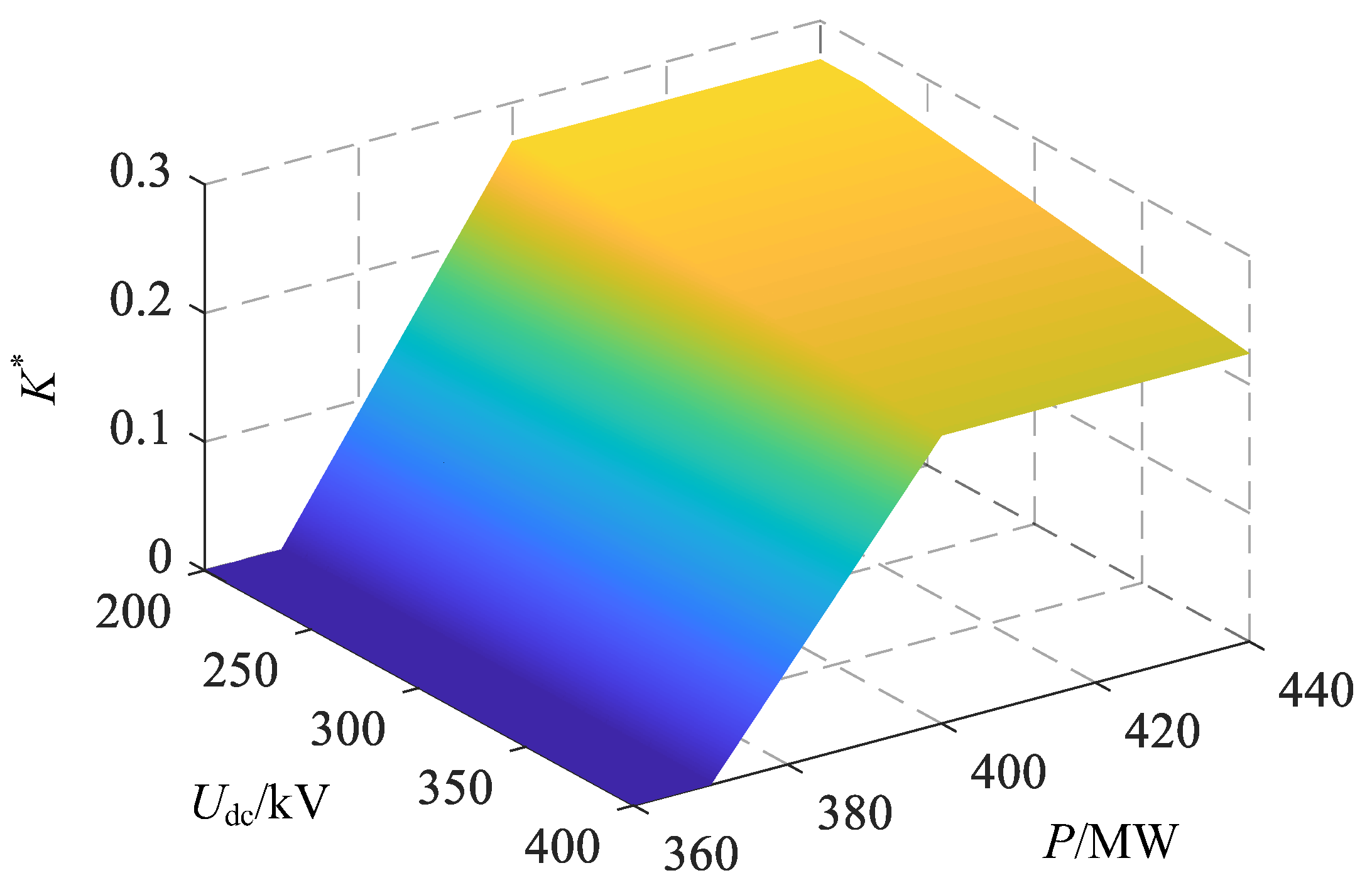
The output surface of the fuzzy controllers is shown in Figure 11.

Figure 11 further illustrates the relationship between the fuzzy inputs and the adaptive droop coefficient. The output surface varies continuously over the whole input domain because the membership functions of FLC1 and FLC2 cover all operating regions and adjacent fuzzy subsets overlap with each other in the transition regions. In the normal operating region, the surface changes slowly, indicating that small fluctuations in active power or DC voltage do not cause significant variations in K^*. In the transition regions, the surface slope increases gradually, which reflects the smooth activation of the power-margin-preservation or DC-voltage-support objective. Near the boundary regions, the Z-shaped and S-shaped membership functions lead to saturated output characteristics, so that the corresponding control objective can be fully activated under extreme operating conditions.

No discontinuous jump or singular point appears on the output surface. This is because at least one membership function remains active for any input value, and the centroid defuzzification method generates a continuous crisp output. Although the local derivative of the surface may change at the junctions of piecewise membership functions, the output value itself remains continuous. Therefore, the adaptive droop coefficient K^* changes smoothly during operating-point switching, which helps avoid abrupt power redistribution and improves the dynamic coordination among operating-loss minimization, converter power-margin preservation, and DC-voltage-deviation suppression.

4. Simulation Verification

A DC system with a VSC-based multi-terminal architecture will evolve into a DC grid when it reaches a certain scale and forms a meshed DC network. Conversely, a meshed DC grid may be converted back to a radial or partially meshed VSC-MTDC system under N − 1 operating conditions. In this research, a five-terminal DC grid model as shown in Figure 1 is built in the electromagnetic transient simulation software PSCAD4.5/EMTDC. Conventional fixed-coefficient droop control is selected as the direct numerical benchmark in the simulation verification because the proposed fuzzy-slope controller is developed by adaptively modifying the droop coefficient within the same decentralized droop control framework. This comparison allows the influence of the fuzzy-slope mechanism itself to be evaluated under identical system topology, converter parameters, line parameters, and disturbance sequences. For other improved droop control strategies reported in the literature, their control objectives, communication requirements, and implementation assumptions are different from those of the proposed method. Therefore, instead of conducting a potentially unfair numerical reproduction, this paper provides a functional comparison with representative advanced droop control strategies and focuses the quantitative simulation comparison on the fixed-coefficient droop benchmark. To clarify the relationship between the proposed method and representative improved droop control strategies, a functional comparison is provided in

Table 4. Functional comparison of different droop control strategies.

Method	Main Objective	Communication	Switching Smoothness	Margin Consideration	Main Limitation
Fixed droop	Power sharing and DC-voltage regulation	No	Limited	Limited	Fixed coefficient cannot adapt to operating-point changes
Voltage-restoration-based strategy	DC-voltage recovery and support	Usually requires coordination	Medium	Not the main focus	Mainly focuses on voltage recovery rather than loss–margin coordination
Nonlinear hybrid droop strategy	Nonlinear power redistribution and overload mitigation	No/low	Medium	Considered under specific overload logic	Switching relationship among multiple objectives is predefined
Proposed fuzzy-slope droop	Loss, margin, and voltage-deviation coordination	No	High	Explicitly considered	Depends on membership-function and rule-base design

.

Therefore, the quantitative simulation comparison in this paper is mainly used to verify whether the proposed fuzzy-slope mechanism improves the fixed-coefficient droop benchmark under the considered multi-objective operating-point switching scenarios.

The simulation verification is organized according to the three control objectives of the proposed fuzzy-slope droop strategy. Case 1 is designed to verify the power-margin preservation capability under heavy-load operating-point switching. Case 2 is designed to verify the operating-loss reduction capability when the converter stations operate near their reference power. Case 3 is designed to verify the DC-voltage support capability under low-voltage or severe operating-point switching conditions. For each case, the proposed fuzzy-slope droop control is compared with conventional fixed-coefficient droop control using the same system topology, converter parameters, line parameters, and disturbance settings. The evaluation indices include DC-voltage deviation, converter active-power redistribution, power-margin utilization, operating loss, and smoothness of operating-point transition.

The rated capacities of S1-S5 are set to 500 MW, 500 MW, 400 MW, 200 MW, and 250 MW, respectively. The base capacity of the DC system is 100 MVA. The rated DC-voltage is ±200 kV, which is taken as the base voltage of the DC system, and the allowable DC voltage fluctuation range of the studied VSC-MTDC system is ±0.1 p.u. Converter stations S1 and S2 employ constant active power control and constant AC voltage control, acting as rectifier stations. The other converter stations employ droop control and constant AC voltage control, serving as inverter stations. Let K₃, K₄, and K₅ be the conventional droop coefficients corresponding to S3, S4, and S5, respectively. The conventional droop coefficients are set inversely proportional to the rated capacity, which are set as K₃ = 0.08, K₄ = 0.16, and K₅ = 0.128. The sum of K₃, K₄, and K₅ remains unchanged after each operating point switching.

4.1. Case 1: Comprehensive Operating-Point Switching Under Power-Reference Changes

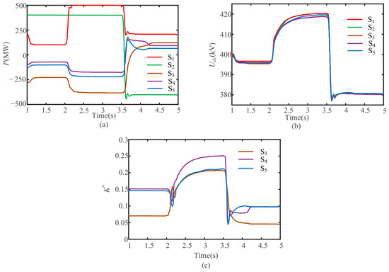
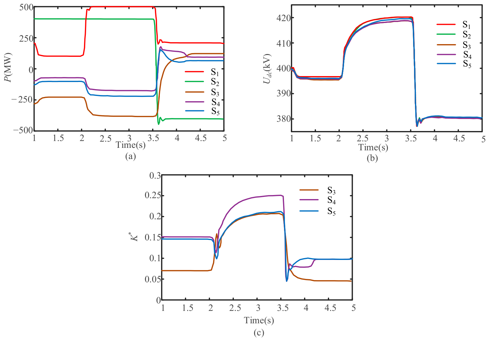
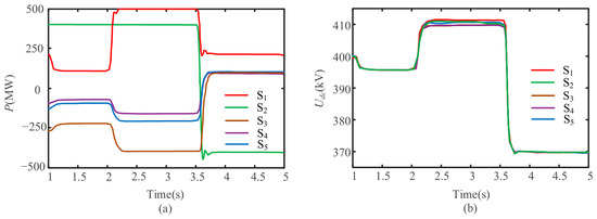
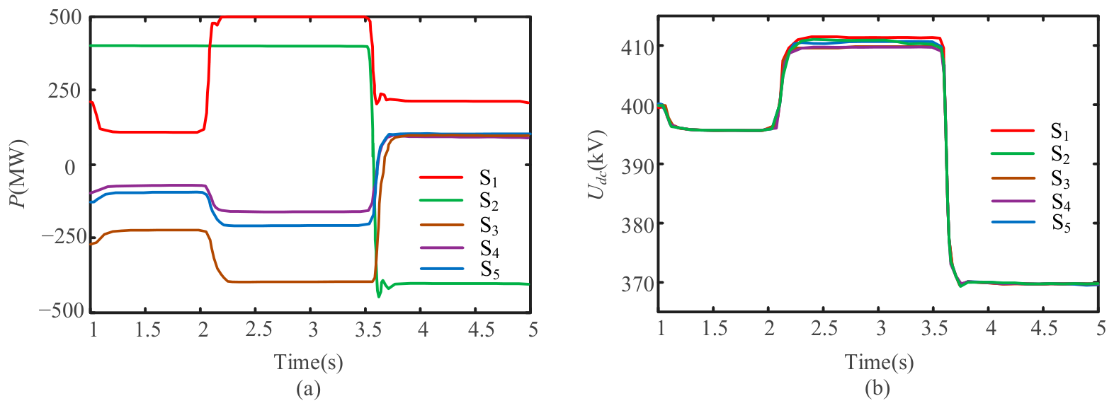
This case is designed to verify the comprehensive operating-point switching capability of the proposed fuzzy-slope droop control under multiple power-reference changes. The verification focuses on whether the proposed controller can coordinate the three control objectives, namely operating-loss minimization, converter power-margin preservation, and DC-voltage-deviation suppression, when the system experiences both load reduction, load increase, and power-flow reversal. The system topology, converter capacities, line parameters, and conventional droop coefficients are kept the same as those described above. Respectively, the initial power references of S₁–S₅ are configured as 210 MW, 400 MW, −280 MW, −100 MW, and −130 MW. At 1 s, the power reference of S₁ is reduced to 100 MW. At 2 s, it is increased to 500 MW. At 3.5 s, the power reference of S₁ returns to 210 MW, and the power flow of S₂ is reversed simultaneously. Converter stations S₃–S₅ use the proposed fuzzy droop control and the conventional droop control, respectively. The simulation results are illustrated in Figure 12 and Figure 13.

The power balance results at the steady state before and after the power reference changes are presented in

Table 5. Fuzzy droop control case 1 power balance results.

Parameter	1.6–2 s	3.1–3.5 s	4.6–5 s
S1 active power	100 MW	500 MW	210 MW
S2 active power	400 MW	400 MW	−400 MW
S3 active power	−218.9 MW	−372.7 MW	133.3 MW
S4 active power	−75.7 MW	−177.4 MW	92.5 MW
S5 active power	−104.6 MW	−222.6 MW	65.1 MW
Total loss	100.8 MW	127.3 MW	100.9 MW

and

Table 6. Traditional droop control case 1 power balance results.

Parameter	1.6–2 s	3.1–3.5 s	4.6–5 s
S1 active power	100 MW	500 MW	210 MW
S2 active power	400 MW	400 MW	−400 MW
S3 active power	−221.1 MW	−400 MW	102.6 MW
S4 active power	−71.3 MW	−155.4 MW	95.7 MW
S5 active power	−93.1 MW	−204.3 MW	109.3 MW
Total loss	114.5 MW	140.3 MW	117.6 MW

.

During 1.6–2.0 s, the power reference of S1 is reduced and the overall loading level of the DC system decreases. In this interval, the fuzzy weighting factor generated by FLC1 gradually decreases, which increases the contribution of the loss-oriented droop coefficient K₁ in K^*. As a result, the system moves toward a loss-minimization operating point. The total operating loss is reduced from 114.5 MW under conventional droop control to 100.8 MW under the proposed control, corresponding to an 11.9% reduction. This verifies that the proposed controller can guide the system toward an economic power-distribution state when sufficient converter power margin is available.

During 3.1–3.5 s, the power reference of S1 is increased to 500 MW, and the receiving-end converter stations operate closer to their power limits. Under conventional fixed-coefficient droop control, S3 absorbs a larger portion of the unbalanced power because it has the smallest droop coefficient. This may reduce its remaining power margin and weaken its subsequent voltage-regulation capability. By contrast, under the proposed fuzzy-slope droop control, FLC1 increases the fuzzy weighting factor α, thereby increasing the contribution of the power-margin-oriented droop coefficient K₂. Consequently, the unbalanced power is redistributed more evenly among S3–S5. At the steady state, the remaining power margins of S3, S4, and S5 are 29.3 MW, 24.6 MW, and 29.4 MW, respectively, which indicates that the converter power-margin preservation objective is effectively activated under heavy-load conditions.

After 3.5 s, the power flow of S2 is reversed for dispatching requirements. This operating-point transition causes a more pronounced DC-voltage deviation. Under conventional droop control, the droop coefficients remain fixed and cannot respond to the low-voltage tendency, resulting in a minimum DC voltage of 370.2 kV after the new steady state is reached. Under the proposed control, FLC2 detects the reduction in the DC-voltage margin and decreases the adaptive droop coefficient through the fuzzy impairment term. Therefore, the system gradually switches to a voltage-support-oriented operating point. The minimum DC voltage increases to 381.4 kV, demonstrating that the proposed controller can improve DC-voltage disturbance rejection during severe operating-point switching. Overall, case 1 confirms that the proposed control strategy can achieve smooth and coordinated switching among loss minimization, power-margin preservation, and DC-voltage-deviation suppression.

4.2. Case 2: Heavy-Load Operating-Point Switching and Power-Margin Preservation

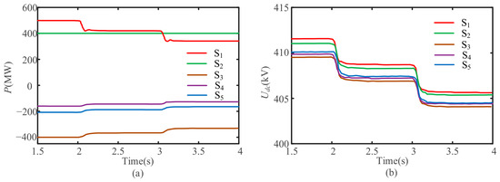
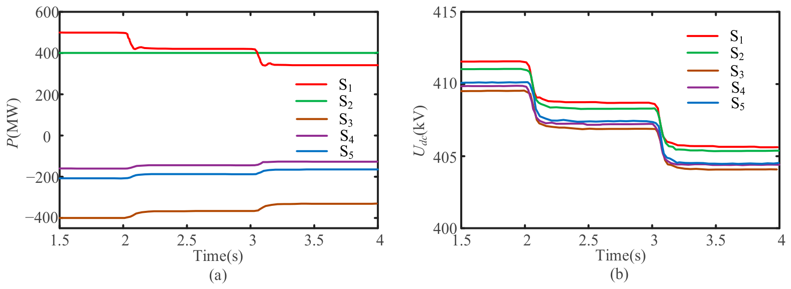
This case is designed to evaluate the performance of the proposed controller under heavy-load operating conditions. The main verification objective is to determine whether FLC1 can guide the droop-controlled converter stations from the loss-oriented operating point to the power-margin-oriented operating point when the receiving-end converter stations approach their power limits. The same five-terminal VSC-MTDC model, converter parameters, line parameters, and conventional droop coefficients are adopted. Respectively, the initial power references of S₁–S₅ are configured as 500 MW, 400 MW, −280 MW, −100 MW, and −130 MW. At 1 s, the power reference of S₁ is reduced to 420 MW. At 2 s, it is further decreased to 320 MW. Converter stations S₁–S₅ use the proposed fuzzy droop control and the conventional droop control, respectively. The simulation results are illustrated in Figure 14 and Figure 15.

The power balance results at the steady state before and after the power reduction are presented in

Table 7. Fuzzy droop control case 2 power balance results.

Parameter	1.6–2 s	2.6–3 s	3.6–4 s
S1 active power	500 MW	420 MW	320 MW
S2 active power	400 MW	400 MW	400 MW
S3 active power	−373.3 MW	−341.4 MW	−296.1 MW
S4 active power	−178.0 MW	−159.2 MW	−143.5 MW
S5 active power	−223.2 MW	−201.3 MW	−182.7 MW
Total loss	125.5 MW	118.1 MW	97.7 MW

and

Table 8. Traditional droop control case 2 power balance results.

Parameter	1.6–2 s	3.1–3.5 s	4.6–5 s
S1 active power	500 MW	420 MW	320 MW
S2 active power	400 MW	400 MW	400 MW
S3 active power	−400 MW	−363.3 MW	−322.0 MW
S4 active power	−158.4 MW	−141.2 MW	−124.1 MW
S5 active power	−204.3 MW	−184.1 MW	−162.2 MW
Total loss	137.3 MW	131.4 MW	111.7 MW

.

The results in Table 7 and Table 8 further demonstrate the effectiveness of the proposed controller under heavy-load operating conditions. Before the power reduction, the receiving-end converter stations operate with relatively small remaining power margins. In this condition, the proposed controller does not simply allocate power according to fixed droop coefficients. Instead, FLC1 evaluates the converter power regulation margin and adjusts the fuzzy weighting factor α, so that the power-margin-oriented objective is considered in the droop coefficient selection. This prevents an individual converter station from undertaking excessive unbalanced power and improves the utilization of the regulation capacity of S3–S5.

After the first power reduction, the operating point enters the transition region of FLC1. The fuzzy weighting factor α changes continuously rather than abruptly, which enables a gradual shift from the power-margin-oriented objective to the loss-oriented objective. After the second power reduction, the loading level of the receiving-end stations is further reduced, and the system has sufficient converter power margin. In this stage, FLC1 accelerates the decrease in α, thereby increasing the contribution of the loss-oriented droop coefficient K₁. This explains why the reduction in total operating loss becomes more significant as the operating point moves away from the heavy-load boundary.

Quantitatively, the total operating loss under the proposed fuzzy-slope droop control is 125.5 MW, 118.1 MW, and 97.7 MW at the three steady-state intervals, whereas the corresponding losses under conventional droop control are 137.3 MW, 131.4 MW, and 111.7 MW. The loss reduction ratios are 8.6%, 10.1%, and 12.5%, respectively. The increasing reduction ratio indicates that the proposed controller can adaptively strengthen the loss-minimization objective when the converter stations regain sufficient power margin. Meanwhile, compared with conventional fixed-coefficient droop control, the active-power distribution among S3–S5 is more balanced, indicating that the proposed strategy can coordinate operating-loss reduction and converter power-margin preservation rather than optimizing only one objective.

4.3. Case 3: Light-Load Operating-Point Switching and DC-Voltage-Deviation Suppression

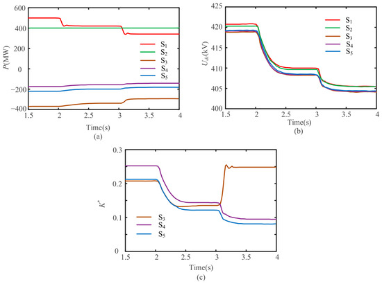
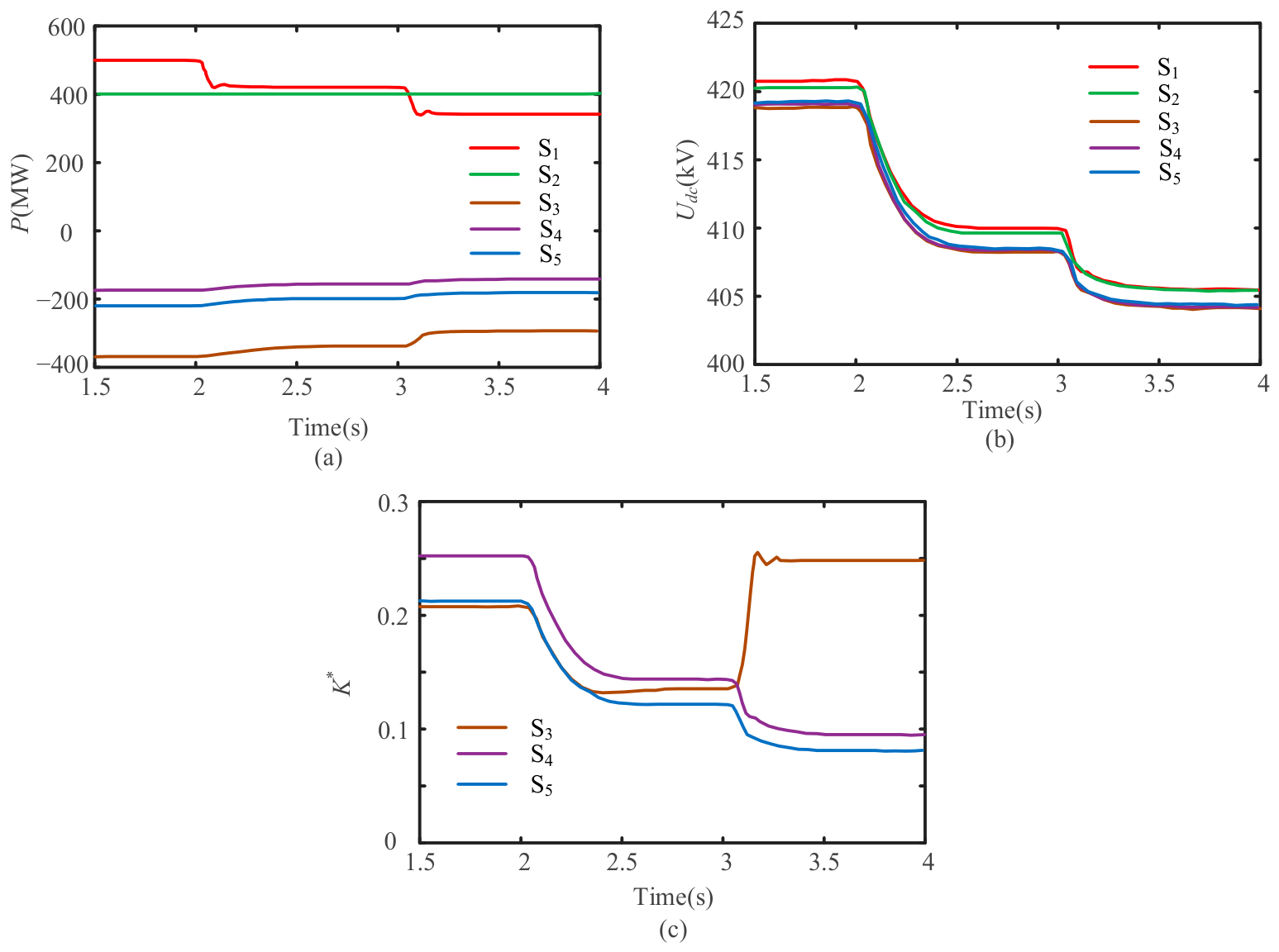
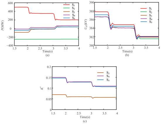
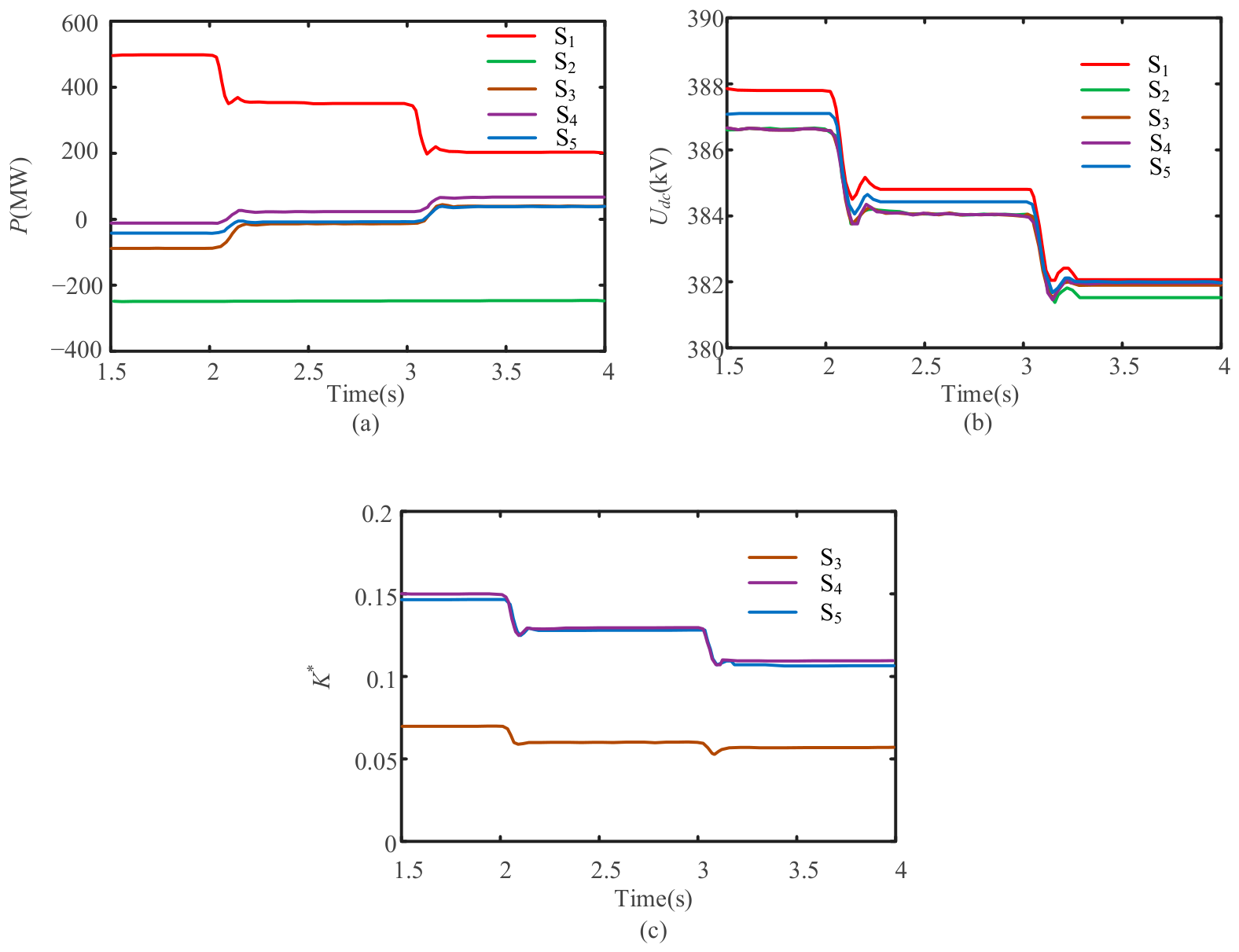
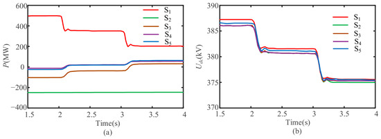
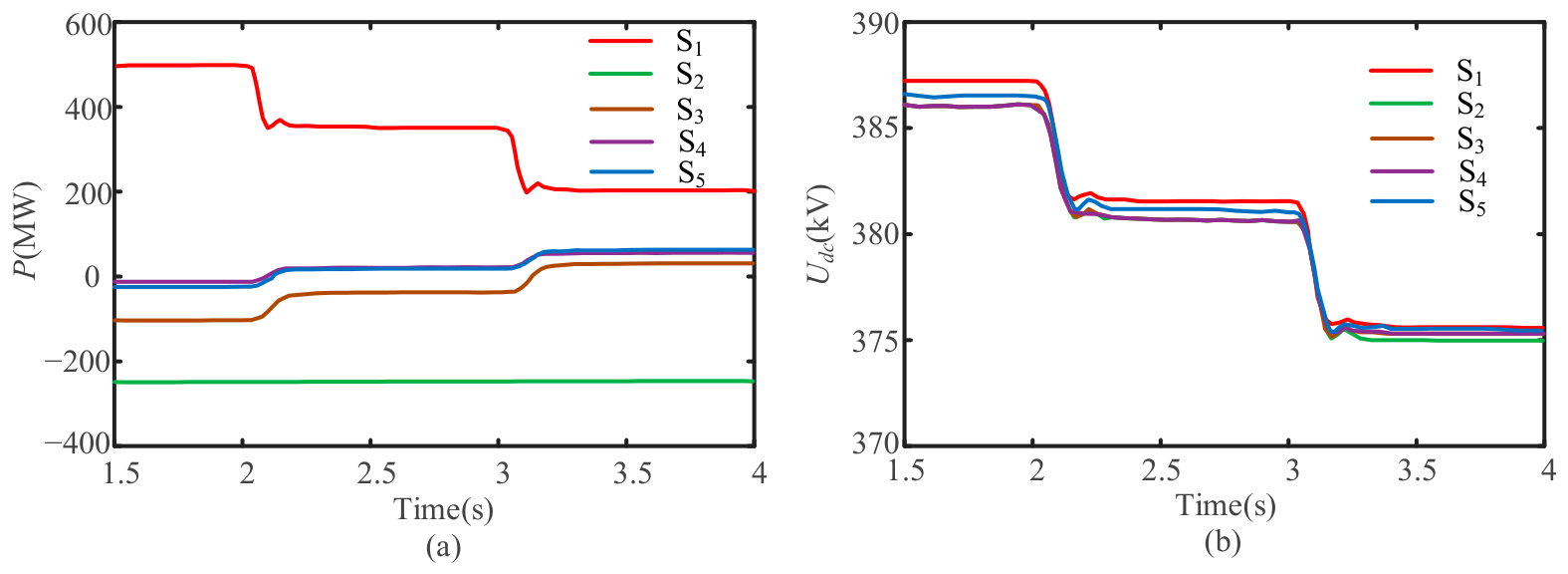
This case is designed to verify the DC-voltage-deviation suppression capability of the proposed controller under light-load operating conditions. The main verification objective is to determine whether FLC2 can reduce the adaptive droop coefficient and strengthen DC-voltage support when the DC voltage approaches the lower admissible range during operating-point switching. The system topology, converter capacities, line parameters, and conventional droop coefficients remain unchanged. Respectively, the initial power references of S₁–S₅ are configured as 500 MW, −250 MW, −280 MW, −100 MW, and −130 MW. At t = 1 s, the power reference of S₁ is reduced to 350 MW, and at t = 2 s, it is further decreased to 200 MW. Converter stations S₃–S₅ use both the proposed fuzzy droop control and the conventional droop control for comparison. The simulation results are illustrated in Figure 16 and Figure 17.

The power balance results of the system under the steady state before and after power reduction are presented in

Table 9. Fuzzy droop control case 3 power balance results.

Parameter	1.6–2 s	3.1–3.5 s	4.6–5 s
S1 active power	500 MW	350 MW	200 MW
S2 active power	−250 MW	−250 MW	−250 MW
S3 active power	−89.8 MW	−13.8 MW	40.5 MW
S4 active power	−12.9 MW	20.6 MW	67.8 MW
S5 active power	−45.8 MW	−8.2 MW	39.1 MW
Total loss	101.5 MW	98.6 MW	97.4 MW

and

Table 10. Traditional droop control case 3 power balance results.

Parameter	1.6–2 s	3.1–3.5 s	4.6–5 s
S1 active power	500	350	200
S2 active power	−250	−250	−250
S3 active power	−103.2	−36.6	32.8
S4 active power	−11.6	22.1	56.5
S5 active power	−24.2	19.9	63.9
Total loss	111.0	105.4	103.2

.

The results in case 3 verify the DC-voltage-deviation suppression capability of the proposed controller under light-load operating conditions. When the power reference of S1 is reduced, the active-power balance of the DC grid changes and the operating point shifts toward a low-voltage region. Under conventional fixed-coefficient droop control, the droop coefficient remains unchanged during the whole switching process. Therefore, the controller cannot distinguish whether the dominant control requirement is loss reduction or DC-voltage support. This limitation leads to a larger DC-voltage deviation during the transition process.

Under the proposed fuzzy-slope droop control, FLC2 takes the DC-voltage margin (U_dc − U_dcmin) as the input and generates the fuzzy output related to the impairment coefficient β. When the DC voltage approaches the lower admissible range, β increases and the equivalent droop coefficient K^* is reduced. According to the droop characteristic, a smaller droop coefficient strengthens the voltage-support capability of the converter station. Therefore, the proposed controller shifts the dominant objective from operating-loss minimization to DC-voltage-deviation suppression when the low-voltage tendency becomes significant.

Compared with conventional droop control, the proposed strategy maintains a higher DC-voltage level throughout the operating-point switching process. This indicates that the voltage-support-oriented objective is effectively activated by FLC2. At the same time, because the fuzzy output changes continuously, the transition of K^* does not introduce an abrupt operating-point jump. Therefore, case 3 demonstrates that the proposed control strategy can improve DC-voltage support under light-load and low-voltage conditions while maintaining smooth active-power redistribution among the droop-controlled converter stations.

To further compile the verification results and make the comparison among the three operating-point switching cases clearer, the main disturbance settings, activated fuzzy controllers, key comparison results, and verified control capabilities are summarized in

Table 11. Summary of simulation verification.

Case	Objective	Disturbance	Activated FLC	Main Result	Verified Function
Case 1	Multi-objective switching	S1 reference changes and S2 power-flow reversal	FLC1 + FLC2	Loss is reduced and minimum DC voltage increases from 370.2 kV to 381.4 kV	Comprehensive coordination
Case 2	Heavy-load coordination	S1 power reference decreases	FLC1	Total loss is reduced by 8.6%, 10.1%, and 12.5%	Loss–margin coordination
Case 3	Low-voltage support	S1 power reference decreases under light-load condition	FLC2	DC voltage remains higher than that under conventional droop control	Voltage-deviation suppression

.

As summarized in Table 11, the three cases verify the proposed fuzzy-slope droop control from different aspects. Case 1 confirms the comprehensive switching capability among multiple control objectives, case 2 demonstrates the coordination between operating-loss reduction and converter power-margin preservation under heavy-load conditions, and case 3 verifies the DC-voltage-deviation suppression capability under light-load conditions. These results indicate that the proposed strategy can continuously adjust the droop coefficient according to the operating state, thereby achieving smoother operating-point transition and better multi-objective coordination than conventional fixed-coefficient droop control.

5. Conclusions

To address the decision-making limitations among control objectives caused by the reliance on accurate mathematical models in conventional multi-objective droop controllers, this work presents a fuzzy-based droop control strategy. A self-coordinating fuzzy droop controller is developed for three steady-state control objectives, namely maintaining the power margin of converter stations, reducing the operating loss of the DC system, and minimizing the DC-voltage deviation. The proposed control strategy comprehensively considers the above three control objectives. It takes the fuzzy weighted average of the droop coefficient obeying the economic power distribution and the droop coefficient considering the power margin, and superimposes a fuzzy reduction coefficient on the average value. Simulation results on the PSCAD4.5/EMTDC platform prove that the fuzzy weighting factor and the fuzzy reduction coefficient are generated by two fuzzy controllers with the active power and DC-voltage as inputs, respectively. This enables the switching of the operating point of the DC system: under heavy-load conditions, the control targets are to maintain the power margin of each VSC station and decrease the operating loss; under light-load conditions, the control targets are to decrease the operating loss and the DC voltage deviation. The switching of each control objective demonstrates the effectiveness of autonomous coordinated decision-making within the transition region.

References

- Guo, C.; Liao, J.; Jiang, Z.; Zhang, X.; He, D. Suppressing Second-Harmonic Transfer via Fractional-Order Notch Filter and Triple-Active-Bridge Power-Flow Controller for Accurate Measurement. IEEE Trans. Instrum. Meas. 2026, 75, 9001814. [Google Scholar] [CrossRef] [Scilit]
- Lin, H.; Liao, J.; Guo, C. Improved Residual Current Detection Method and Protection Scheme for Double-Circuit Bipolar LVDC System Based on Modal Transformation. IEEE Trans. Instrum. Meas. 2026, 75, 3505012. [Google Scholar] [CrossRef] [Scilit]
- Sun, K.; Xiao, H.; Liu, Y. Optimized allocation method of the VSC-MTDC system for frequency regulation reserves considering ancillary service cost. CSEE J. Power Energy Syst. 2022, 8, 53–63. [Google Scholar] [CrossRef] [Scilit]
- Mohamed, H.R.A.; Mohamed, Y.A.-R.I.; El-Saadany, E.F. Analysis and Dynamic Stabilization of a High-Voltage VSC-MTDC Grid with DC Power Flow Controller Connected to Extremely Weak AC Systems. IEEE Open J. Power Electron. 2024, 5, 718–736. [Google Scholar] [CrossRef] [Scilit]
- Latorre, H.F.; Ghandhari, M.; Söder, L. Active and reactive power control of a VSC-HVdc. Electr. Power Syst. Res. 2008, 78, 1756–1763. [Google Scholar] [CrossRef] [Scilit]
- Beerten, J.; Cole, S.; Belmans, R. Modeling of Multi-Terminal VSC HVDC Systems with Distributed DC Voltage Control. IEEE Trans. Power Syst. 2014, 29, 34–42. [Google Scholar] [CrossRef] [Scilit]
- Porst, J.; Luther, M.; Baumann, S.; Hahn, C. Energy Droop Control for MMC based Multiterminal HVDC Systems. In Proceedings of the 2019 IEEE Milan PowerTech, Milan, Italy, 23–27 June 2019; pp. 1–6. [Google Scholar] [CrossRef] [Scilit]
- Tavakoli, S.D.; Sanchez-Sanchez, E.; Prieto-Araujo, E.; Gomis-Bellmunt, O. DC Voltage Droop Control Design for MMC-Based Multiterminal HVDC Grids. IEEE Trans. Power Deliv. 2020, 35, 2414–2424. [Google Scholar] [CrossRef] [Scilit]
- Sekhavatmanesh, H.; Ferrari-Trecate, G.; Mastellone, S. Optimal Adaptive Droop Design via a Modified Relaxation of the OPF. IEEE Trans. Control Syst. Technol. 2023, 31, 497–510. [Google Scholar] [CrossRef] [Scilit]
- Lv, J.; Zhang, J.; Zhi, Y.; Wang, K.; Ge, P.; Zhang, J.; Li, Q. Cooperative Control Method Based on Two-Objective Co-Optimization for MMCs in HVDC Systems. Processes 2025, 13, 1839. [Google Scholar] [CrossRef] [Scilit]
- Wang, Y.; Qiu, F.; Liu, G.; Lei, M.; Yang, C.; Wang, C. Adaptive Reference Power Based Voltage Droop Control for VSC-MTDC Systems. J. Mod. Power Syst. Clean Energy 2023, 11, 381–388. [Google Scholar] [CrossRef] [Scilit]
- Farrokhabadi, M.; Canizares, C.A.; Simpson-Porco, J.W.; Nasr, E.; Fan, L.; Mendoza-Araya, P.A.; Tonkoski, R.; Tamrakar, U.; Hatziargyriou, N.D.; Lagos, D.; et al. Microgrid Stability Definitions, Analysis, and Examples. IEEE Trans. Power Syst. 2020, 35, 13–29. [Google Scholar] [CrossRef] [Scilit]
- Liu, C.; Liu, H.; Jiang, S.; Zheng, L. Dynamic Frequency Support and DC Voltage Regulation Approach for VSC-MTDC Systems. CSEE J. Power Energy Syst. 2023, 9, 645–658. [Google Scholar] [CrossRef] [Scilit]
- Liu, Q.; Wang, Y.; Wang, S.; Liang, D.; Zhao, Q.; Zhao, X. Voltage Regulation Strategy for DC Distribution Networks Based on Coordination of Centralized Control and Adaptive Droop Control. IEEE Trans. Power Deliv. 2022, 37, 3730–3739. [Google Scholar] [CrossRef] [Scilit]
- Sun, P.; Wang, Y.; Khalid, M.; Blasco-Gimenez, R.; Konstantinou, G. Steady-state power distribution in VSC-based MTDC systems and dc grids under mixed P/V and I/V droop control. Electr. Power Syst. Res. 2023, 214, 108798. [Google Scholar] [CrossRef] [Scilit]
- Ye, Z.; Guo, C.; Liao, J.; Wang, Y. Improved droop control strategy for an MMC-MTDC connected to offshore wind farms with dynamic correction of the actual operating point. Int. J. Electr. Power Energy Syst. 2023, 152, 109277. [Google Scholar] [CrossRef] [Scilit]
- Wang, Y.; Wen, W.; Wang, C.; Liu, H.; Zhan, X.; Xiao, X. Adaptive voltage droop control of multiterminal VSC-HVDC systems for DC voltage deviation and power sharing. IEEE Trans. Power Deliv. 2019, 34, 169–176. [Google Scholar] [CrossRef] [Scilit]
- Shadabi, H.; Kamwa, I. Dual adaptive nonlinear droop control of VSC-MTDC system for improved transient stability and provision of primary frequency support. IEEE Access 2021, 9, 76806–76815. [Google Scholar] [CrossRef] [Scilit]
- Liu, Y.; Green, T.C.; Wu, J.; Rouzbehi, K.; Raza, A.; Xu, D. A New Droop Coefficient Design Method for Accurate Power-Sharing in VSC-MTDC Systems. IEEE Access 2019, 7, 47605–47614. [Google Scholar] [CrossRef] [Scilit]
- Li, M.; Yang, H.; Zhao, R.; Dong, N.; Lu, Y.; Wang, C. Fuzzy-logic-based coordinated control strategy for flexible multi-state switches. Autom. Electr. Power Syst. 2021, 45, 35–42. [Google Scholar] [CrossRef]
- Chen, X.; Wang, L.; Sun, H.; Chen, Y. Fuzzy Logic Based Adaptive Droop Control in Multiterminal HVDC for Wind Power Integration. IEEE Trans. Energy Convers. 2017, 32, 1200–1208. [Google Scholar] [CrossRef] [Scilit]
- Abazari, A.; Dozein, M.G.; Monsef, H.; Wu, B. Wind turbine participation in micro-grid frequency control through self-tuning, adaptive fuzzy droop in de-loaded area. IET Smart Grid 2019, 2, 301–308. [Google Scholar] [CrossRef] [Scilit]
- Shifa, F.A.; El Moursi, M.S.; Khadkikar, V. Fuzzy-Adaptive Droop Gain Selection for Enhanced Frequency Support and DC Voltage Regulation in MTDC System. IEEE Trans. Power Syst. 2025, 40, 2310–2323. [Google Scholar] [CrossRef] [Scilit]
- Nguyen, V.T.K.; Wu, Y.-K.; Phan, Q.D. Adaptive Droop Control for Compromise Between DC Voltage and Frequency in Multi-Terminal HVDC. IEEE Access 2021, 9, 131708–131719. [Google Scholar] [CrossRef] [Scilit]
- Hussaini, H.; Yang, T.; Bai, G.; Urrutia-Ortiz, M.; Bozhko, S. A Low-Complexity Artificial Neural Network-Based Optimal Droop Gain Design Strategy for DC Microgrids Onboard the More Electric Aircraft. IEEE Trans. Transp. Electrif. 2024, 10, 7310–7327. [Google Scholar] [CrossRef] [Scilit]
Disclaimer/Publisher’s Note: The statements, opinions and data contained in all publications are solely those of the individual author(s) and contributor(s) and not of MDPI and/or the editor(s). MDPI and/or the editor(s) disclaim responsibility for any injury to people or property resulting from any ideas, methods, instructions or products referred to in the content. |
© 2026 by the authors. Licensee MDPI, Basel, Switzerland. This article is an open access article distributed under the terms and conditions of the Creative Commons Attribution (CC BY) license.