


Abstract
Software effort estimation (SEE) serves as a cornerstone of effective software project management, and case-based reasoning (CBR) stands out as one of the most extensively adopted approaches within this domain. Nevertheless, CBR-based SEE models are still plagued by two critical challenges: conventional case retrieval mechanisms lack the ability to differentiate the relative importance of various features, and data scarcity remains a persistent bottleneck. Both issues significantly compromise the estimation accuracy and interpretability of the models. To address these limitations, we propose a SHAP–Mixup synergistic framework that enhances both feature-aware similarity learning and data distribution modeling. Specifically, we introduce (1) a stability-aware SHAP-weighted similarity metric that integrates both the magnitude and variance of feature contributions to improve retrieval robustness, and (2) a density-aware Mixup augmentation strategy that generates synthetic samples guided by local data manifold structure rather than random interpolation. Experimental results on seven benchmark datasets demonstrate that the proposed method reduces MAE and MSE by up to 20.2% on average compared to baseline CBR models, while consistently improving Pred(0.25). Furthermore, by enhancing model interpretability, the proposed method equips project managers with actionable insights into the key drivers of software effort, thereby facilitating more informed and efficient resource allocation. Building on these findings, this study provides a novel and effective pathway for developing SEE models that are more accurate, robust, and transparent.
1. Introduction
As a fundamental component of software engineering, software effort estimation (SEE) aims to quantify the human effort required for successful project completion. This effort is typically measured using standard units such as person-hours, person-days, or person-months [1]. The accuracy of these estimations exerts a critical influence on project outcomes [2]. For instance, overestimation can lead to inefficient resource allocation and inflated project costs, whereas underestimation often results in schedule overruns, degraded software quality, and even project failure. These risks have been widely documented in prior studies [3,4,5,6]. Consequently, reliable SEE is instrumental in controlling development costs, ensuring software quality, facilitating effective project monitoring, and safeguarding an organization’s reputation [7].
SEE approaches can be broadly categorized into two primary types: expert-based methods and data-driven methods [7]. Expert-based methods rely on the knowledge and experience of domain experts to estimate the effort required for new projects. However, these methods are highly susceptible to subjective biases, which may arise from cognitive limitations, individual experience, anchoring effects, and inconsistent judgment among experts. Such biases can lead to systematic estimation errors and reduced reproducibility [8]. In contrast, data-driven methods leverage historical project data and mathematical models to generate estimates, which are more objective and reproducible. This data-driven approach can be further divided into algorithm-based and machine learning-based sub-methods. Algorithm-based methods, such as the Constructive Cost Model (COCOMO) [9] and Function Point Analysis (FPA) [10], quantify software size through statistical modeling and calculate effort using empirical formulas [11]. Despite their wide adoption in SEE practices, these methods have limited applicability in the early stages of a project. During this phase, project information is often sparse, and the scope of potential requirement changes cannot be accurately determined [2]. Machine learning-based approaches address some limitations of traditional methods by automatically learning feature patterns from data, thereby offering greater flexibility and estimation accuracy. However, a key drawback of most machine learning models is their poor interpretability [12].
Lee et al. [13] developed a framework based on the Least Modification Principle (LMP) within CBR to estimate software project modification effort. By selecting 17 key influencing factors and computing effort according to LMP, they streamlined the case-adaptation process, thereby improving estimation accuracy and efficiency. Phannachitta [14] employed CBR to estimate software project effort and combined meta-heuristic algorithms with machine learning techniques to optimize case adaptation. Gradient boosting machines, together with conventional adaptation strategies, enhanced CBR’s ability to accommodate differences between new and historical projects, thereby increasing estimation accuracy. Brady et al. [15] proposed the W system, which integrates CBR with contrast-set learning to improve software development effort estimation. W retrieves cases via CBR and applies contrast-set learning to identify attributes that distinguish efficient from inefficient projects, and then recommends appropriate adjustment strategies. Mustyala and Bisi [16] used the harmony search algorithm to automatically explore optimal CBR parameter configurations and validated the approach on 13 public software datasets. Hameed et al. [2] suggested optimising key CBR parameters, such as feature selection, feature weighting, similarity measures, and the number of k-nearest neighbours, using a genetic algorithm (GA) to produce highly accurate effort estimates for software projects.
The aforementioned studies demonstrate that CBR-based models can markedly improve the accuracy and efficiency of software effort estimation and exhibit strong adaptability across estimation tasks in diverse domains and project types. Despite these advances, two fundamental limitations remain insufficiently addressed. First, existing CBR-based SEE models rely on heuristic or static feature weighting schemes, which fail to capture the instance-dependent contribution of features. Second, current data augmentation strategies neglect the intrinsic structure of SEE data, often introducing distributional bias due to random sampling. These limitations jointly restrict both the reliability of similarity computation and the generalization ability of the model. In fact, the judicious selection and optimization of features are critical for enhancing the adaptation efficiency and accuracy of CBR models. Redundant features, or those unrelated to the target variable, may confound computation and degrade system performance. Moreover, because the individual contribution of each feature to the decision is often not explicitly quantified, the interpretability of some models remains limited. Consequently, feature optimization has become a pivotal step in strengthening both the predictive capability and the interpretability of CBR-based effort-estimation models.
SHAP, developed by Lundberg and Lee [17], are grounded in game-theoretically optimal Shapley values; they effectively quantify each feature’s contribution to model predictions and enhance interpretability [18], and have therefore attracted increasing attention. Fan et al. [19] applied SHAP to magnetoencephalography (MEG) signal prediction, resolving the ambiguity of feature attribution in high-dimensional settings. Wang et al. [20] combined SHAP with XGBoost and k-means clustering to identify key features in hydrological forecasting, thereby improving both interpretability and predictive accuracy. Mostofi et al. [21] employed SHAP in multi-criteria decision making (MCDM) to quantify the contribution of sub-criteria to higher-level criteria, capture interdependencies among sub-criteria, and strengthen decision stability and consistency. Liu et al. [22] introduced SHAP values for feature selection in a Parkinson’s disease dataset and, together with four classifiers, achieved a diagnostic model with markedly improved interpretability and performance. Li et al. [23] employed SHAP to examine how land-surface temperature and environmental factors influence near-surface air-temperature estimation, offering insights for urban heat-island research and temperature-prediction optimization. These studies show that SHAP has been widely adopted across disciplines and holds substantial value for feature optimization and interpretability analysis, yet its application to SEE remains limited. In this study, we introduce SHAP into SEE to refine feature-weight computation, thereby significantly improving the CBR model’s interpretability.
Because SEE datasets are typically small, the effectiveness of feature optimization may be limited; to enhance optimization stability, we further introduce data-augmentation techniques to enlarge the sample set. Mixup, a widely used data-augmentation method, has shown strong performance in numerous domains [24,25,26]. However, conventional Mixup generates new samples via random sampling [27], which can cause the synthetic data to drift from the original distribution and thus undermine its credibility. To address this issue, we propose a sampling strategy that leverages feature-neighborhood density information so that the synthetic samples better conform to the original data structure, thereby improving the reliability of the augmented cases.
To address the limitations of existing CBR models in handling SEE data, this paper proposes a SHAP-weighted and Mixup-based data-augmentation approach to improve the accuracy and robustness of CBR in SEE. The main contributions of this study are as follows:
- A stability-aware SHAP-weighted similarity metric: Unlike conventional feature weighting methods that rely on global importance or heuristic tuning, the proposed method incorporates both the magnitude and variance of SHAP values, enabling robust and adaptive feature weighting across heterogeneous instances.
- Density-based Mixup Augmentation: We introduce two significant improvements over the standard Mixup approach: (1) a neighborhood-density sampling strategy that replaces random pairing with a more targeted selection of parent cases, and (2) an adapter model-based mechanism for generating synthetic decision values. Together, these enhancements produce higher-fidelity synthetic samples, substantially improving the model’s robustness, especially in data-scarce scenarios.
- A synergistic framework: We are the first to design and validate a framework that combines a SHAP-guided retrieval mechanism with an enhanced Mixup data augmentation technique. Our experiments reveal a powerful synergy between the two components, where the performance of the integrated model surpasses the individual contributions of each part.
- Comprehensive empirical validation: Experiments on seven public datasets against five mainstream machine learning models confirm the superior effectiveness, robustness, and generalizability of the proposed framework.
This paper is structured as follows: Section 2 reviews preliminary knowledge, after which Section 3 details our proposed approach. Section 4 then presents the experimental results to validate its performance, and Section 5 concludes with a summary of our findings and potential avenues for future research.
2. Proposed Method
2.1. CBR Framework
Originating in cognitive science, CBR is a problem-solving paradigm that closely mirrors human cognitive processes [28]. Its core principle is to address new problems by leveraging past knowledge and experiences. Notably, CBR not only explains how a solution is derived but is also capable of incremental learning [29]. When a novel problem case arises, a CBR system typically retrieves the K most similar cases from the case base and reuses their solutions to address the new problem. If the recommended solution proves unsuitable, the system enters the revision stage, where the solution is adjusted accordingly. Once the correctness of the final solution is verified, the new case together with its solution is stored in the case base for future use. A standard CBR cycle comprises five stages: representation, retrieval, reuse, revision, and retention. Figure 1 provides a concise overview of this workflow. This cycle demonstrates the incremental learning capability of CBR. By continuously accumulating and updating the case base, the system dynamically refines its reasoning performance, endowing CBR with marked adaptability and scalability.
Figure 1.
The “4R” Cycle Process of CBR.
2.2. Stability-Aware SHAP Feature Weighting
2.2.1. SHAP Computation
In our implementation, SHAP values are computed in each training fold using a tree-based regression model as the explanation target (LightGBM by default) together with the TreeExplainer algorithm. Unless otherwise specified, the background dataset consists of a random subset of 100 training samples. For large datasets, SHAP values are calculated on a stratified subsample of the training fold to reduce computational overhead while preserving the distribution of the effort values. Let the SEE dataset be denoted as
where n is the number of software projects and each instance contains d features. For each instance i, SHAP provides local explanation values representing the contribution of feature k to the predicted effort.
2.2.2. Stability-Aware SHAP Weighting
Although SHAP values provide reliable local explanations, directly using the average SHAP importance may lead to unstable feature weighting because some features exhibit large fluctuations across instances. To address this issue, we introduce a stability-aware SHAP weighting mechanism that jointly considers the magnitude and stability of feature contributions. First, the global importance of feature k is measured using the mean absolute SHAP value:
where represents the overall predictive contribution of feature k across the dataset. Next, to capture the variability of feature contributions, we compute the standard deviation of absolute SHAP values:
A large indicates that the contribution of feature k varies significantly across different projects, while a smaller value implies a more stable influence. To jointly incorporate importance and stability, we define the stability-aware importance score as
where is a small positive constant used to avoid division by zero. Finally, the normalized feature weight is obtained as
where denotes the final weight assigned to feature k, satisfying . This formulation can be interpreted as a variance-regularized importance estimation, where features with high contribution but low stability are down-weighted. This is conceptually related to robust feature selection and metric learning, ensuring that similarity computation is less sensitive to instance-level fluctuations.
2.2.3. SHAP-Weighted Similarity Computation
To improve the estimation accuracy of the CBR system, the derived SHAP weights are incorporated into the similarity computation used during case retrieval. Let two SEE cases be defined as and . The SHAP-weighted similarity between them is defined as
where denotes the similarity function and is the feature weight vector. To comprehensively evaluate similarity between projects, three classical similarity measures are adopted. The SHAP-weighted Euclidean similarity is defined as
The SHAP-weighted Manhattan similarity is
The SHAP-weighted grey relational similarity is defined as
where denotes the target project and represents the i-th historical project. The variables and denote the normalized values of the k-th feature. For the grey relational similarity, we define
and is the distinguishing coefficient, which is set to by default. These similarity measures can be viewed as different instantiations of a weighted distance metric, where SHAP-derived weights define a feature-wise scaling, analogous to a diagonal Mahalanobis distance. By integrating stability-aware SHAP weights into similarity computation, features with higher predictive importance and more stable contributions exert stronger influence on case similarity. This mechanism improves the robustness of case retrieval and ultimately enhances the accuracy of SEE.
2.3. Density-Aware Mixup for SEE Data Augmentation
SEE tasks frequently suffer from data scarcity. Given that CBR derives solutions from historical cases, its effectiveness depends heavily on the quality and diversity of training data. Consequently, data augmentation has emerged as a critical preprocessing step for effort-estimation datasets. By generating diversified training samples, augmentation enhances a model’s adaptability to heterogeneous scenarios and perturbed data. Mixup, proposed by Zhang et al. [30], has garnered considerable interest in this field; its core idea is to generate synthetic samples by proportionally mixing two training instances and their corresponding labels through linear interpolation.
The conventional Mixup technique generates new samples through interpolation between cases selected randomly from the case base [31]. However, this random sampling approach risks introducing anomalous or outlier samples, thereby compromising the effectiveness of data augmentation. To mitigate the interference from such anomalous data, this paper proposes a novel sampling strategy based on nearest-neighbor density information within the feature space. This strategy aims to generate virtual cases that better conform to the true data distribution, enhancing the reliability of the augmented dataset.
Given a historical case dataset , where n denotes the total number of cases in the case base, represents the i-th SEE case, is its set of input features, and is the output feature (representing software effort). The probability of sampling the case is then defined as
where represents the index set of the k-nearest neighbors for case in the feature space, and k denotes the preselected neighbor parameter. As indicated by Equation (12), ; a smaller average distance between case and its k-nearest neighbors corresponds to a higher local density, thereby reducing the likelihood of being an outlier. This formulation approximates a kernel density estimation in the feature space, where samples located in high-density regions receive higher sampling probability. As a result, the generated synthetic samples are more likely to lie on the underlying data manifold, reducing the risk of distributional shift. Consequently, this mechanism directly increases the sampling probability of case . After case is sampled, the probability of sampling case is defined as
where denotes the scale parameter of the Gaussian kernel in the feature space. For computational simplicity, is set to the median of . As shown in Equation (13), the sampling process is biased toward assigning a higher probability to the nearest neighbors of case . Consequently, the augmented case set is strategically concentrated in regions with high neighborhood density. This approach thus achieves two objectives: it not only increases the sample size but also enhances the reliability of case information simultaneously. After selecting parent cases and , our method generates a new augmented case by interpolating their respective attributes.
Our augmentation process begins by interpolating the feature attributes, a step consistent with conventional Mixup. However, we introduce a key innovation for the output features: instead of interpolation, it is generated using a predictive model. Specifically, we first train an adaptation model on the historical case set to learn the mapping from features to the decision. This trained model then ingests the interpolated feature attributes to predict the final decision attribute for the new case. The primary advantage of this predictive method over simple interpolation is a significant reduction in interpolation error. This enhances the reliability and adaptability of the augmented cases, which ultimately leads to improved training accuracy in subsequent adaptation models. This augmentation process for generating a new case, , is formally defined as follows:
where is the mixing coefficient sampled from a Beta distribution with parameters and . The choice of and controls the diversity of synthetic samples. Smaller values lead to more extreme interpolation, while larger values generate samples closer to the original data distribution. denotes the predictive adaptation model previously trained on the historical case set. and represent the feature vector and corresponding decision attribute of the new augmented case, respectively.
Compared to conventional Mixup that linearly interpolates labels, the proposed model-based label generation reduces interpolation bias by leveraging a learned mapping function. This is particularly important in SEE tasks where the relationship between features and effort is highly nonlinear. Algorithm 1 outlines the complete step-by-step procedure for our Mixup-based sample augmentation, which incorporates the case generation logic defined above.
In summary, in scenarios of data scarcity within a CBR case base, Mixup can be employed to expand the case set and broaden its coverage, thereby enhancing the performance of subsequent modeling and analysis.
| Algorithm 1 Mixup-based case augmentation for software effort estimation. |
| Require: Historical case base: (where : case, : feature vector, : software effort); Beta-distribution hyperparameters: ; Pre-trained adaptation model on : ; Target number of augmented samples: . |
| Ensure: Augmented case set: |
| 1: for to Q do |
| 2: // Step 1: Sample two parent cases with density-aware probability |
| 3: Sample following |
| 4: Sample following |
| 5: // Step 2: Mixup interpolation on feature space |
| 6: Sample mixing coefficient: |
| 7: Compute augmented feature vector: |
| 8: // Step 3: Estimate effort for augmented case |
| 9: Predict software effort: |
| 10: // Step 4: Add augmented case to the set |
| 11: Construct augmented case: |
| 12: Update augmented set: |
| 13: end for |
| 14: return |
3. Improved CBR for SEE
Based on the CBR framework and the aforementioned methods, this study proposes an enhanced CBR approach for software effort estimation. It integrates two key strategies: data augmentation to improve case-base quality and a feature optimization technique to improve retrieval accuracy. Our approach comprises three key steps: data preprocessing, case retrieval, and case adaptation, as depicted in the workflow of Figure 2. When faced with a new SEE task, the system sequentially executes these three steps to generate the final estimation result.
Figure 2.
Main Steps of the CBR cycle.
(1) Data Preprocessing: This stage aims to enhance the quality and coverage of the case-base through a model-guided data augmentation process. Specifically, after training a predictive model on historical data to act as a labeling oracle, we generate synthetic cases by performing a modified Mixup: first selectively pairing cases based on their neighborhood density, then interpolating their features, and finally employing the pre-trained model to predict the corresponding target effort.
(2) Case Retrieval: This step identifies the most relevant historical cases for a new target case. To achieve this, we first derive feature weights by calculating and normalizing the Shapley values for each feature, a process guided by a selected machine learning model and the SHAP method. These weights are then integrated into a weighted k-nearest neighbor (k-NN) algorithm to compute the similarity between the target case and each historical case. Finally, only those cases exceeding a predefined similarity threshold are retrieved to form the final similar-case set.
(3) Case Adaptation: In this stage, the retrieved similar-case set is used to generate a precise effort estimate for the target case. The process begins by using the similar-case set as a dedicated training dataset to train a specialized adaptation model, which is designed to learn the specific mapping between feature attributes and the target variable (i.e., software effort) within this localized data context. Subsequently, the feature attributes of the target case are fed into this newly trained model, and its output provides the final effort estimate.
4. Experiment and Discussion
4.1. Research Questions
Despite recent advances in CBR-based SEE models, two critical research gaps remain: (1) the lack of adaptive and interpretable feature weighting mechanisms, and (2) the insufficient consideration of data distribution in augmentation strategies. To address these gaps, this study formulates the following research questions aligned with our objectives:
RQ1: Can the proposed SHAP-based weighting scheme improve the estimation accuracy of CBR models for SEE? Furthermore, do weights derived from SHAP values demonstrate robust applicability and stability across different contexts?
RQ2: What is the impact of incorporating the proposed Mixup-based sample augmentation technique on the predictive performance of CBR models?
RQ3: Does combining the proposed SHAP weighting scheme and Mixup technique synergistically improve the performance of CBR models for SEE, in terms of both estimation accuracy and model robustness, beyond what is achievable by either technique in isolation?
4.2. Datasets and Evaluation Metrics
To evaluate the performance of our proposed approach, we conducted a series of experiments on seven publicly available SEE datasets, summarized in Table 1. These datasets were sourced from two widely-used benchmarks in SEE research: datasets 1–5 were obtained from the PROMISE repository [32,33], while datasets 6 and 7 were constructed from the ISBSG data repository [34,35]. The PROMISE datasets are publicly available and widely used benchmarks in SEE research. The ISBSG dataset used in this study is one of the most recent publicly accessible releases at the time of experimentation. Although some datasets contain historical projects, they remain representative due to their diversity and scale. Collectively, this selection of datasets spans a broad spectrum of project types, scales, and feature dimensions, thereby providing a comprehensive foundation to evaluate the effectiveness and generalizability of our approach.
Table 1.
Description of the benchmark datasets for software effort estimation.
The ISBSG data repository encompasses 11,848 software projects from diverse organizations worldwide, featuring 233 distinct attributes. Its vast scale and high heterogeneity necessitate a systematic filtering process to yield a suitable subset for analysis. Therefore, in accordance with the official ISBSG data usage guidelines, we performed the following steps to extract such a subset:
(1) Data quality: Adhering to the recommendations from ISBSG and the related literature [36,37], we exclusively retained projects that met stringent quality criteria: a ‘Data Quality’ rating of ‘A’ or ‘B’ and a ‘UFP Rating’ of ‘A’.
(2) Resource level: To align with prior studies [38], our analysis focuses exclusively on development-team effort. Therefore, we filtered for projects with a ‘Resource Level’ of ‘1’. According to ISBSG definitions, this specific level isolates the core development effort, excluding subsequent contributions from support, maintenance, and end-user teams that are included in higher levels.
(3) Development type: Given the marked differences in development processes and cost structures between ‘New Development’ and ‘Enhancement’ projects, we analyzed them as two distinct cohorts to ensure a more accurate and valid evaluation.
(4) Function-size counting approach: Following ISBSG guidelines to ensure the comparability of functional size metrics across all projects, our dataset includes ‘New Development’ projects measured with either IFPUG V4+ or the comparable NESMA standard, and ’Enhancement’ projects measured solely with IFPUG V4+.
(5) Normalized ratio filter: In accordance with ISBSG recommendations, we calculated a “Normalized Ratio” for each project to serve as a data quality indicator. This ratio, defined as the standardized effort divided by the originally reported effort, cannot be less than 1.0 by definition. We then excluded projects with a ratio exceeding 1.2, as such a value indicates both significant data uncertainty and limited analytical value.
This five-step preparation process resulted in two distinct datasets: a new-development set (ISBSG-I, n = 603) and an enhancement set (ISBSG-II, n = 1028).
Public datasets present several challenges for analysis, including missing values, a lack of standardization, and diverse feature types (e.g., categorical, range, and interval values). To address these issues and prepare the data for our experiments, we executed the following preprocessing steps:
(1) Feature Selection: We performed according to the guidelines of [36,37] to identify the most relevant variables.
(2) Scalar Conversion: For features defined by a single bound, values were estimated by multiplying a lower bound by a factor of 1.1 or an upper bound by a factor of 0.9. For features defined by an interval, their value was taken as the midpoint of the bounds.
(3) Categorical Encoding: Multi-class categorical variables were encoded using a multi-label binarizer, while single-class categorical variables were transformed via one-hot encoding.
(4) Missing Value Imputation: A random forest algorithm was employed to impute any remaining missing values.
(5) Standardization: Finally, all numerical features in the datasets were standardized to ensure a common scale. This process yielded the final, analysis-ready datasets used in our study.
We employed a 5-fold cross-validation (CV) to evaluate model performance. In each fold, the dataset was partitioned into an 80% training set and a 20% test set. The model was trained on the former and evaluated on the latter, with the final performance metrics computed by averaging the results across all five folds. The number of modeling features and the sample size for each dataset are detailed in Table 1.
To comprehensively evaluate model performance, we adopt five widely used evaluation metrics: MMRE, MdMRE, MAE, MSE, and Pred(0.25). These metrics cover complementary perspectives: MMRE and MdMRE reflect the robustness of relative errors; MAE and MSE quantify the magnitude of absolute errors; and Pred(0.25) measures prediction accuracy within a practical acceptance threshold. Collectively, they enable a thorough and reliable performance assessment, consistent with mainstream practices in software effort estimation. The formal definitions of these metrics are given below:
where denotes the actual effort of the i-th project or test case, is the corresponding effort estimated by the model, and n represents the total number of test cases. refers to the relative error of the i-th project. The metric calculates the proportion of projects for which .
To ensure reproducibility, all hyperparameters used in the proposed SHAP–Mixup CBR framework are explicitly reported in this section. The density-aware Mixup strategy employed a Beta distribution, , to generate interpolation coefficients. In this study, we set and , following common practice, to encourage diverse interpolation. The number of synthetic samples generated per query instance was controlled by the parameter . The neighborhood size for density estimation was set to . SHAP values were computed using a background dataset sampled from the training data. The background size was fixed at 100 instances to balance computational efficiency and estimation accuracy. To improve stability, SHAP values were averaged over multiple sampling runs. The number of retrieved similar cases was set to unless otherwise specified. The similarity threshold was set to 0.85 to filter out weakly related cases. All hyperparameters were determined based on preliminary experiments and fixed across all datasets to ensure fair comparison. No dataset-specific tuning was performed.
4.3. RQ1: Evaluating the Effectiveness and Stability of SHAP-Based Weighting in CBR
4.3.1. Impact of SHAP-Based Weighting on CBR Performance
Our experimental procedure was designed to evaluate the impact of a SHAP-based feature weighting strategy on the performance of a CBR system for SEE. The core of the experiment involved comparing the CBR model’s performance under two weighting schemes: unweighted and SHAP-weighted.
For the unweighted scheme, we adopted three conventional similarity measures: Euclidean distance (Euc), Manhattan distance (Man), and grey relational degree (Gre). For the SHAP-weighted scheme, we first calculated the SHAP value of each feature to quantify its importance. These values were then normalized and utilized as feature weights. Subsequently, the weights were incorporated into the standard similarity measures to derive three weighted variants, SHAP-Euc, SHAP-Man, and SHAP-Gre, whose detailed computation is presented in Section 2.2.3.
For all six similarity measures, the k-nearest neighbor (k-NN) algorithm was utilized to retrieve the most similar cases from the case base. The final prediction for a target case was then computed as the similarity-weighted average of the solutions from these neighboring cases. Figure 3 illustrates this complete estimation procedure, and the mathematical formulations for the six similarity measures are provided below.
Figure 3.
The CBR estimation workflow for unweighted and SHAP-weighted approaches.
The experiments were conducted on three datasets: China, ISBSG-I, and ISBSG-II. These datasets were selected for their large sample sizes and significant feature diversity, which provide greater stability for k-NN-based case retrieval. Following a series of preliminary experiments for parameter tuning, the number of nearest neighbors k was set to 9 to optimize estimation performance.
Table 2, Table 3 and Table 4 present the estimation performance of the CBR method on the test sets of the three selected datasets. The results are detailed for both the unweighted and the SHAP-weighted strategies across all six similarity measures previously described.
Table 2.
Performance evaluation of different similarity measures on the China dataset.
Table 3.
Performance evaluation of different similarity measures on the ISBSG-I dataset.
Table 4.
Performance evaluation of different similarity measures on the ISBSG-II dataset.
Analysis of the results presented in Table 2, Table 3 and Table 4 reveals that the application of SHAP-based feature weighting consistently enhances the estimation performance of the CBR model. This enhancement is observed across all three datasets, regardless of the base similarity measure employed. Notably, the optimal similarity measure proved to be dataset-dependent. For instance, SHAP-Gre yielded the best performance on the China dataset, while SHAP-Euc was the top performer on the ISBSG-I dataset. On the ISBSG-II dataset, SHAP-Man delivered the most accurate results for the majority of metrics. Crucially, however, the top-performing model in every scenario was a SHAP-weighted variant, outperforming its corresponding unweighted counterpart. This universal superiority underscores the robustness and high adaptability of the proposed weighting strategy, showcasing its capability to augment model performance across diverse data contexts.
4.3.2. Stability and Consistency Analysis of SHAP-Derived CBR Feature Weights
To comprehensively evaluate the proposed SHAP-based weighting approach, this section presents a two-stage experimental study conducted on the China dataset. First, we adopted an XGBoost model to visualize and interpret the importance and influence of individual features. Then, we verified the general effectiveness and applicability of the proposed method by testing it across five classical machine learning models.
In this preliminary analysis, we employed an XGBoost model as the adaptation engine within the CBR framework. To improve the stability of SHAP-based feature attributions, the Mixup data augmentation technique was applied to the training set with an expansion factor of 3. SHAP values were then calculated for each feature based on the augmented data and normalized to be used as weighting coefficients. A detailed description of the features is provided in Table 5; DevType represents the type of software development activity, typically categorized as “New Development”, “Enhancement”, or “Maintenance”. This variable reflects differences in development complexity, resource requirements, and cost structures. The analytical results are visualized in Figure 4 and Figure 5. Figure 4 shows a SHAP summary plot, in which features are sorted vertically by their mean importance. For each feature, individual points represent samples, and their horizontal positions denote the corresponding SHAP values, indicating the direction and magnitude of the feature’s impact. The SHAP heatmap in Figure 5 visualizes the marginal effect of each feature, where red denotes a positive contribution to the predicted effort and blue denotes a negative contribution.
Table 5.
Feature descriptions for the China dataset.
Figure 4.
SHAP summary plot for the China dataset.
Figure 5.
SHAP heatmap plot for the China dataset.
Figure 4 reveals that AFP, Added, PDR-UFP, and PDR-AFP are the most influential features for software effort estimation in the China dataset. As a core measure of project size, AFP positively correlates with development effort. Added, the number of new functional points, directly drives up project workload by necessitating additional development and testing tasks. Furthermore, PDR-UFP and PDR-AFP, which represent productivity delivery rates, demonstrate a logical inverse relationship with effort; lower productivity implies higher cost per unit, thus increasing total project effort. The strong influence of these features suggests that similarity searches in CBR should prioritize them, a process that can be significantly enhanced by our SHAP-based weighting.
Figure 5 provides a more granular view of these feature contributions across individual projects. It shows that AFP and Added consistently yield positive SHAP values for most samples, a finding that aligns with their high overall importance in Figure 4 and indicates their stable, effort-increasing impact. In contrast, the productivity-related features, PDR-UFP and PDR-AFP, exhibit significant variation, reflecting their strong sensitivity to project-specific contexts. This variability, however, is consistent with their underlying logic: for projects with low productivity, their SHAP values tend to be positive, increasing the predicted effort; conversely, for high-productivity projects, their negative SHAP values reflect a marginal contribution to reducing effort.
Notably, the feature importance hierarchy identified by the SHAP model is not merely a statistical artifact but also aligns strongly with established principles in software engineering. The finding that projects with larger feature sizes and lower productivity require more resources is consistent with practical experience, thereby validating the credibility and interpretability of our SHAP-based approach.
To validate the robustness of our SHAP-based weighting strategy, we first examined its consistency across different predictive models. As presented in Figure 6, we generated SHAP value heatmaps for five distinct models (LightGBM, XGBoost, RF, GBR, and SVR). The results reveal a high degree of consistency in feature importance rankings, despite the underlying differences in the models’ learning mechanisms. This stability demonstrates that SHAP provides a reliable basis for feature attribution, justifying its use as a generalized weighting strategy independent of any specific adaptation algorithm.
Figure 6.
Heatmap of normalized feature importance for China dataset across different machine learning models.
Building on the established reliability of SHAP, we then conducted a comprehensive evaluation to determine its effectiveness in improving prediction performance. We used the same five machine learning models and compared their performance on the China dataset before and after applying the SHAP weights. The comparison was conducted across the previously defined suite of evaluation metrics. Figure 6 summarizes these results, where “Mean Performance” represents the aggregated average of the normalized metric scores to reflect the overall change in predictive capability. As illustrated in Figure 7, the introduction of the SHAP weighting mechanism yielded significant performance enhancements. All five weighted models outperformed their unweighted counterparts in key error metrics such as MSE, MAE, MMRE, and MdMRE, indicating a consistent reduction in prediction bias and sensitivity to outliers. The performance gains were particularly pronounced for the RF and GBR models in the MMRE metric and for the XGBoost model in the MSE metric. Furthermore, the Pred(0.25) metric, which measures prediction acceptability, improved across all models. This uniform improvement across diverse models and metrics confirms that the SHAP-based strategy effectively enhances model accuracy and reliability.
Figure 7.
Impact of SHAP weighting on performance across models on the China dataset.
In conclusion, our analysis provides a definitive positive answer to RQ1. We first established that the SHAP-based feature importance ranking is both remarkably stable across models and consistent with domain knowledge. We then demonstrated that integrating these robust, SHAP-based weights into the CBR model leads to significant and widespread improvements in predictive performance. Therefore, the SHAP-based weighting strategy proves its strong applicability and cross-model robustness in software effort estimation by consistently enhancing the CBR model’s performance.
4.4. RQ2: Evaluating the Effects of Mixup Augmentation on the Predictive Performance of CBR Models
4.4.1. Effect of Mixup Augmentation on CBR Performance
The performance of a CBR system in SEE is fundamentally dependent on the quantity and quality of its historical case-base. To validate our improved Mixup-based augmentation strategy, we conducted experiments on seven datasets, comparing the CBR system’s performance before and after augmentation across multiple adaptation models. Through preliminary experiments guided by each dataset’s sample size, we optimized the augmentation multiple to balance model generalization gains against the risks of noise introduction and data distribution distortion. These tailored augmentation multiples are detailed in Table 6. The comprehensive results across all models and datasets are presented in Table 7, Table 8 and Table 9.
Table 6.
Sample augmentation multiples for each dataset.
Table 7.
Performance comparison before and after augmentation based on LightGBM model.
Table 8.
Performance comparison before and after augmentation based on SVR model.
Table 9.
Performance comparison before and after augmentation based on XGBoost model.
Table 7 shows that the Mixup strategy enhances the predictive performance of the LightGBM-based CBR system, as supported by quantitative metrics. This is evident in the MAE results, with reductions observed in six out of seven datasets. For instance, in the Desharnais dataset, the MAE decreases from 1.243 to 0.811, corresponding to a 34.8% relative reduction. A similar improvement in prediction accuracy is reflected in the Pred(0.25) metric, which is enhanced in six datasets. Furthermore, the strategy’s positive impact on model robustness is supported by improved MSE, MMRE, and MdMRE values in five datasets. Overall, the mean values across all metrics confirm that the Mixup-augmented model generally outperforms the unaugmented baseline, indicating clear advantages in controlling overall error and improving generalization.
Analysis of Table 8 revealed the impact of the Mixup strategy on the SVR-based CBR system. Its influence was most consistent on the MAE metric, which improved across all seven datasets. For instance, in the China dataset, the MAE dropped from 0.313 to 0.245, a 21.7% relative reduction. Performance was also enhanced for MSE, MdMRE, and Pred(0.25) in six datasets. In contrast, the MMRE metric improved in only three datasets, a result possibly influenced by the SVR model’s sensitivity to data scaling. Overall, the mean values across metrics confirmed that the Mixup-augmented model outperforms the baseline in four of the five key metrics, indicating its potential utility in enhancing the overall performance of the SVR-based system.
Analysis of Table 9 detailed the effects of the Mixup strategy on the XGBoost-based CBR system. Performance improved MSE, MAE, and MMRE in six of seven datasets (particularly for Cocomo81, China, and ISBSG-I), and MdMRE in four. Notably, the Pred(0.25) metric improved in only two datasets, suggesting a potential trade-off where the strategy enhances overall error control at the expense of local predictive precision. The mean values across the datasets confirmed the augmented model’s superiority on the MSE, MAE, and MMRE metrics, reinforcing its value in enhancing overall error control for the XGBoost model.
4.4.2. Applicability and Stability Analysis of Mixup Augmentation for CBR
To assess the stability and generalizability of our proposed Mixup strategy, we evaluated its performance across five CBR models: LightGBM, XGBoost, RF, GBR, and SVR. The China dataset served as an experimental dataset to test the strategy’s adaptability to challenges like prediction complexity, limited samples, and skewed feature distributions. Performance was compared before and after applying the strategy using the same five metrics: MAE, MSE, MMRE, MdMRE, and Pred(0.25). Figure 8 summarizes the results, where “Mean Performance” refers to the average metric value across all five models for each metric.
Figure 8.
Impact of our proposed mixup across models on the China dataset.
As shown in Figure 8, our proposed Mixup strategy effectively enhanced the performance of all five models under challenging conditions, such as limited samples and skewed feature distributions. The strategy led to a broad reduction in prediction error, evidenced by lower overall MSE and MAE values. This improvement was particularly substantial for the MSE of LightGBM, SVR, and XGBoost. Furthermore, enhancements were observed across other key metrics: LightGBM, SVR, and RF improved both MdMRE and Pred(0.25), with LightGBM’s gain on MdMRE being the most significant. Concurrently, LightGBM and XGBoost achieved lower MMRE values. This comprehensive benefit is confirmed by the mean values, where the four error metrics declined while Pred(0.25) rose, signifying a simultaneous improvement in both model accuracy and high-precision prediction capability.
In answer to RQ2, our findings suggest that our proposed Mixup strategy generally enhances the overall performance of the models and contributes to their predictive stability. While the magnitude of this enhancement may be contingent on specific data characteristics and model selection, the collective results support our proposed Mixup as a viable and effective data augmentation technique for software effort prediction.
4.5. RQ3: Investigating the Synergistic Impact of SHAP and Mixup on CBR Performance
Having established the independent effects of the SHAP weighting and Mixup strategies, this section investigates their potential synergy when applied in combination. To this end, the experiment systematically compares the model performance under four strategies: (1) a baseline model without optimization (Baseline); (2) the SHAP strategy in isolation (SHAP only); (3) the Mixup strategy in isolation (Mixup only); (4) the combined SHAP and Mixup strategy (SHAP + Mixup).
To provide a comprehensive answer to RQ3, we evaluated the results from two complementary perspectives. First, we conducted a macro-level comparison using radar charts. This format excelled at integrating multiple metrics to offer an intuitive, at-a-glance view of each strategy’s overall strengths and trade-offs. We plotted the average performance of all five models across five key metrics on four datasets, an approach that neutralized model-specific biases to provide a fair and holistic assessment of each strategy’s general applicability. Second, we performed a micro-level quantitative analysis using detailed tables for the remaining three datasets. This allowed for a fine-grained comparison between the SHAP+Mixup and Baseline strategies, precisely quantifying the performance gains for each model and metric.
4.5.1. Comparative Performance Analysis: Single Versus Combined SHAP and Mixup Strategies
Figure 9a–d illustrate the comparative performance of the four strategies on the China, COCOMO81, Desharnais, and ISBSG-I datasets, respectively. To ensure a uniform visual interpretation where a larger area consistently signifies better performance, all error-based metrics (MdMRE, MMRE, MAE, MSE) were inverted. In the charts, these are denoted by a “–” prefix (e.g., –MSE). The benefit-based metric, Pred(0.25), is presented without modification as it naturally aligns with this principle.
Figure 9.
Radar chart comparison of average performance for the four strategies across different datasets.
As illustrated in Figure 9a for the China dataset, the SHAP+Mixup strategy demonstrates clear superiority by occupying the largest coverage area and leading on four of the five metrics, with the most significant gains on –MSE and –MAE. Although it is slightly outperformed by SHAP only on –MMRE, it still far surpasses the Baseline and Mixup only strategies. An analysis of the individual strategies reveals that SHAP only surpasses the Baseline across all metrics, while Mixup only also yields considerable improvements, especially on –MSE, –MAE, and –MdMRE. This collectively indicates that while both strategies are individually beneficial, their combination produces the most comprehensive performance enhancement.
On the COCOMO81 dataset, the findings from Figure 9b reinforce the superiority of the SHAP+Mixup strategy. It exhibits the largest radar area and secures top performance on three error metrics: MSE, MAE, and MMRE. The SHAP only strategy also performs well, leading on MdMRE and Pred(0.25) and surpassing the Baseline on all metrics, which highlights its standalone effectiveness. In contrast, the contribution of Mixup only is more modest, outperforming the Baseline on MMRE but matching it on Pred(0.25). Therefore, while SHAP only leads on certain metrics, the combined strategy’s superior performance on the majority of error metrics and its larger overall coverage establish it as the most robust solution for this dataset.
For the Desharnais dataset (Figure 9c), the SHAP+Mixup strategy continues its strong performance, showing the largest radar area and leading on four key metrics. The –MMRE metric shows more mixed results, where even the Baseline achieves a competitive score. Nevertheless, the individual strategies each offer distinct advantages: SHAP only markedly improves Pred(0.25), while Mixup only excels at reducing overall error (–MSE and –MAE). The SHAP+Mixup approach successfully integrates these respective strengths. Consequently, by leading on the majority of key error metrics and delivering the most comprehensive gains, it reaffirms its position as the superior strategy.
The results from the ISBSG-I dataset (Figure 9d) confirm SHAP+Mixup’s superiority, marked by its significantly larger radar area. Both individual strategies are highly effective: SHAP only surpasses the Baseline across all metrics and leads on –MdMRE and Pred(0.25), while Mixup only delivers significant gains on –MMRE, –MAE, and –MSE. The combined strategy effectively integrates these strengths, securing top performance on the three key error metrics, with a particularly commanding lead on –MMRE. This demonstrates a clear synergistic effect; while SHAP only excels on certain metrics, the combined approach provides the most balanced and robust performance, confirming it as the superior overall strategy.
In summary, SHAP+Mixup consistently emerges as the superior strategy across all four datasets, achieving the largest radar coverage and leading on the majority of key metrics. Its success stems from a clear synergistic effect: it combines the individual strengths of SHAP only and Mixup only to produce more stable and comprehensive improvements while mitigating their weaknesses. This establishes the combined approach not merely as an incremental improvement, but as a robust and broadly applicable solution for enhancing CBR models.
4.5.2. Evaluating the Synergistic Effect of SHAP-Mixup over Baseline
Table 10 and Table 11 further quantify the performance of the SHAP+Mixup strategy against the Baseline. The comparison covers the three remaining datasets (ISBSG-II, NASA93, and Miyazayi) across all five CBR models and five key evaluation metrics. Optimal values in the tables are highlighted in bold.
Table 10.
Performance comparison of SHAP+Mixup and baseline strategies on Nasa93.
Table 11.
Performance comparison of SHAP+Mixup and baseline strategies on Miyazayi.
As shown in Table 10 for the NASA93 dataset, the SHAP+Mixup strategy consistently outperforms the Baseline. It delivered substantially lower errors across most models. For instance, LightGBM’s MSE was reduced by 25.6% and its MAE by 31.6%. The strategy also achieved the best MdMRE in four models, indicating improved robustness, and led on MMRE and Pred(0.25) in three models, highlighted by a 42.5% increase in XGBoost’s Pred(0.25). The average metrics confirm this trend, with SHAP+Mixup surpassing the Baseline on all five dimensions to enhance overall accuracy and reliability.
The results for the Miyazayi dataset, presented in Table 11, demonstrate the clear superiority of the SHAP+Mixup strategy. It delivered significant reductions in MSE and MAE for four models, exemplified by a 56.7% drop in XGBoost’s MAE. The strategy also enhanced stability by leading on MdMRE in three models and achieved top performance on Pred(0.25) across all five. Despite a limited advantage on MMRE, the average metrics confirm its overall strength, securing optimal results on four of the five key dimensions and thereby validating its effectiveness in enhancing model performance.
As presented in Table 12, the results on the ISBSG-II dataset reveal the overwhelming superiority of the SHAP+Mixup strategy. It decisively outperformed the Baseline across all models, highlighted by extraordinary error reductions such as a 97.8% decrease in SVR’s MSE and 91.5% in LightGBM’s MAE. Prediction accuracy saw similarly massive gains, with Pred(0.25) for LightGBM and SVR soaring to 0.942 and 0.934, respectively. The average metrics further confirm this comprehensive dominance, substantiating the strategy’s power to both enhance the accuracy and reliability of CBR models and achieve transformative performance on specific datasets. In summary, the consistent findings from Figure 9 and Table 10 and Table 12 unequivocally substantiate the marked superiority of the SHAP+Mixup strategy over the Baseline. This directly answers RQ3 by demonstrating the strategy’s effectiveness in concurrently enhancing the prediction accuracy, reducing various errors, and improving the output stability of CBR models.
Table 12.
Performance comparison of SHAP+Mixup and baseline strategies on the ISBSG-II.
4.6. Ablation Study on the Individual and Synergistic Contributions of SHAP and Mixup
To further address RQ3 and explicitly quantify the individual and joint contributions of the proposed components, we conducted a comprehensive ablation study. Unlike the previous radar-chart-based comparison, this section provides a controlled and quantitative decomposition of performance gains, enabling a rigorous evaluation of the synergistic effect between the stability-aware SHAP weighting and the density-aware Mixup augmentation.
4.6.1. Experimental Design
We evaluated four model configurations under identical experimental settings:
- Baseline: Standard CBR without SHAP weighting and without Mixup augmentation.
- SHAP-only: CBR with stability-aware SHAP weighting.
- Mixup-only: CBR with density-aware Mixup augmentation.
- SHAP+Mixup: The full proposed framework.
All experiments were conducted using 5-fold cross-validation across the seven benchmark datasets. The same evaluation metrics (MSE, MAE, MMRE, MdMRE, and Pred(0.25)) are used to ensure consistency with previous sections.
4.6.2. Gain Decomposition Method
To quantitatively assess the contribution of each component, we define the performance improvement (gain) with respect to the Baseline model. For error-based metrics (MSE, MAE, MMRE, MdMRE), improvement is defined as a reduction in value, while for Pred(0.25), improvement corresponds to an increase.
Let denote a performance metric. The gain of each configuration is defined as
To explicitly measure synergy, we define:
A positive Synergy value indicates that the combined model achieves improvements beyond the additive contributions of its individual components, thereby demonstrating a true synergistic effect.
4.6.3. Quantitative Results and Analysis
Table 13 presents the average gains across all datasets for the MAE and MSE metrics.
Table 13.
Gain decomposition of SHAP and Mixup contributions (average over 7 datasets).
From Table 13, several important observations can be made:
- Both components independently improve performance. SHAP-only consistently reduces prediction error by improving feature weighting, while Mixup-only enhances generalization through data augmentation.
- The joint model achieves the largest improvement. The SHAP+Mixup configuration yields the highest gain across all metrics, confirming the effectiveness of integrating both strategies.
- Positive synergy is consistently observed. The Synergy term is positive for both MAE and MSE, indicating that the combined improvement exceeds the sum of individual gains. This demonstrates that SHAP and Mixup are not merely complementary, but mutually reinforcing.
4.6.4. Interpretation of the Synergistic Mechanism
The observed synergy can be explained from both data-level and feature-level perspectives:
- Feature-level enhancement (SHAP): The stability-aware SHAP weighting improves the reliability of similarity computation by emphasizing features that are both important and stable.
- Data-level enhancement (Mixup): The density-aware Mixup strategy enriches the training distribution by generating high-quality synthetic samples aligned with the data manifold.
- Interaction effect (Synergy): The augmented data produced by Mixup provides a richer and smoother feature space, which in turn stabilizes SHAP value estimation. Conversely, improved SHAP weights guide more meaningful neighborhood structures for Mixup sampling.
This bidirectional interaction leads to a closed-loop enhancement mechanism, where each component amplifies the effectiveness of the other.
4.7. Statistical Significance Analysis
To further validate whether the observed performance improvements are statistically significant, we conducted non-parametric statistical tests based on the experimental results. Given that the performance distributions across datasets may not satisfy normality assumptions, the Wilcoxon signed-rank test was adopted to compare the proposed SHAP-Mixup method against the Baseline strategy. For each dataset, we used the averaged performance values as paired observations. The significance level was set to . Applying the Wilcoxon signed-rank test yielded the following results in Table 14, the results indicate that the improvements achieved by the SHAP-Mixup method over the Baseline are statistically significant for both MAE and MSE.
Table 14.
Wilcoxon signed-rank test results (SHAP-Mixup vs. Baseline).
5. Discussion
Although the experimental results demonstrate the effectiveness of the proposed SHAP–Mixup framework, a deeper positioning of its contributions within the broader SEE literature is essential.
First, compared with traditional CBR-based SEE approaches that rely on heuristic or meta-heuristic feature weighting—such as genetic algorithms [39], harmony search [40], particle swarm optimization, or differential evolution-based tuning—our method introduces a fundamentally different paradigm grounded in explainable machine learning. Existing approaches typically learn global or dataset-level feature weights, which assume that feature importance is stationary across all projects. However, prior studies (e.g., [41,42,43,44]) have shown that SEE datasets are highly heterogeneous, with varying project characteristics and context-dependent drivers. In contrast, our stability-aware SHAP weighting mechanism leverages instance-level feature attribution derived from Shapley values, as formalized in interpretable ML frameworks [45,46]. By further incorporating variance regularization, our approach aligns with recent advances in robust feature selection and metric learning, where stability is treated as a critical factor in generalization. This enables the model to capture both importance and consistency of features, which is largely overlooked in prior SEE studies. Consequently, our method extends SHAP from a purely interpretability tool to a functional component in similarity learning, bridging a gap between explainability and predictive modeling.
Second, in terms of data augmentation, existing SEE research has paid relatively limited attention to systematic data generation techniques, often relying on resampling or noise injection. In broader machine learning domains, Mixup [47] and its variants (e.g., Manifold Mixup [48], AdaMixup [49]) have demonstrated strong generalization capabilities by enforcing linear behavior between samples. However, these methods assume that linear interpolation in feature space preserves semantic validity, which may not hold in SEE due to complex, nonlinear relationships between software attributes and effort. As highlighted in recent studies on structure-aware augmentation, ignoring data distribution can lead to manifold intrusion and unrealistic synthetic samples. Our density-aware Mixup strategy directly addresses this limitation by introducing local density estimation and distance-constrained sampling, conceptually related to kernel density estimation and manifold learning techniques. Furthermore, replacing label interpolation with a predictive model is consistent with recent trends in model-based augmentation and semi-supervised learning, where labels are generated through learned mappings rather than simple convex combinations. Compared with standard Mixup [26,27,28,29], our method is therefore better aligned with the intrinsic structure of SEE data, improving both reliability and generalization.
Third, the primary novelty of this study lies in the systematic integration of explainability-driven feature weighting and distribution-aware data augmentation, which has not been explored in prior SEE literature. Existing studies typically treat feature optimization (e.g., feature selection, weighting) and data augmentation as independent preprocessing steps. However, recent machine learning research suggests that data quality and feature representation are inherently coupled. In our framework, SHAP-based weighting enhances the metric space used for case retrieval, while density-aware Mixup improves the data distribution within that space. This creates a closed-loop enhancement mechanism: improved data leads to more reliable SHAP estimation, and improved feature weighting leads to more meaningful similarity-based learning. The experimental results (Section 4.5) confirm that this interaction is not merely additive but synergistic, yielding consistent improvements across multiple datasets and models. Such synergy is rarely reported in SEE studies, where improvements are often limited to single components.
From a practical standpoint, the integration of SHAP also addresses a long-standing limitation of machine learning-based SEE models—namely, their lack of interpretability. Prior works have noted that black-box models (e.g., ensemble methods, deep learning) often achieve high accuracy at the cost of transparency. By contrast, SHAP provides fine-grained, instance-level explanations that allow practitioners to identify key cost drivers, such as functional size (AFP) and productivity-related metrics. This aligns with research in decision-support systems, where interpretability is critical for trust and adoption. Therefore, our approach not only improves predictive performance but also enhances its usability in real-world project management contexts.
Despite these contributions, several limitations should be acknowledged. The computational overhead associated with SHAP value estimation—particularly in high-dimensional datasets—remains a challenge, as also noted in prior SHAP-related studies. Although the proposed Mixup strategy improves data quality, its effectiveness may depend on the choice of hyperparameters (e.g., neighborhood size, interpolation distribution), which warrants further investigation. While our experiments cover multiple benchmark datasets, SEE data in industrial environments may exhibit additional complexities, such as concept drift and evolving project characteristics. Future work should therefore explore scalable SHAP approximations, adaptive augmentation strategies, and online learning frameworks to further enhance applicability in real-world scenarios.
6. Conclusions
In this study, we proposed a synergistic SHAP+Mixup strategy to address the dual challenges of data sparsity and the need for precise, interpretable feature weighting in CBR-based software effort estimation. Our approach first leverages a refined Mixup technique to augment the dataset, and then applies SHAP to derive precise, interpretable weights for optimizing case retrieval. Comprehensive experiments confirmed the strategy’s marked superiority over both baseline and single-strategy models. The findings demonstrate that our integrated approach significantly enhances the accuracy, reliability, and robustness of effort estimation, showcasing strong generalizability across diverse datasets and machine learning algorithms while improving model interpretability. This provides a robust pathway to advance project management from a reliance on traditional, experience-based models toward more precise, data-driven decision-making. Despite the effectiveness of the proposed SHAP–Mixup framework, its computational overhead may limit scalability in large-scale software effort estimation scenarios. The repeated computation of SHAP values is computationally expensive, and the density-aware Mixup strategy further increases data volume through synthetic sample generation, leading to higher memory and processing demands. To address these challenges, future work will explore distributed and parallel computing strategies. In particular, the Distributed Shared Memory (DSM) paradigm [48] provides a promising solution by enabling seamless integration of distributed resources under a unified shared-memory interface. By leveraging DSM-based architectures, key components of the framework—including SHAP computation, case retrieval, and Mixup augmentation—can be parallelized across multiple nodes. This would improve scalability for large datasets such as ISBSG-II, while preserving the interpretability and accuracy advantages of the proposed method.
In the future, we will focus on enhancing the proposed SHAP+Mixup framework. Its performance can be improved by integrating feature selection techniques prior to SHAP analysis enhance computational efficiency and interpretive clarity. We will also further refine the Mixup strategy with novel techniques such as adaptive mixing coefficients and manifold-aware interpolation to improve its stability. In addition, validating the strategy’s generalizability on a wider range of private industrial datasets is an important direction worth investigating.
Author Contributions
J.L.: Conceptualization, Formal analysis, Methodology, Investigation, Software, Writing—original draft, Writing—review and editing. H.Z.: Software, Writing—original draft, Writing—review and editing. S.S.: Methodology, Project administration, Supervision. M.L.: Data curation, Formal analysis, Resources, Writing—review and editing. S.L.: Funding acquisition, Resources, Writing—review and editing. C.Z.: Validation, Visualization, Investigation, Data curation. K.L.: Data curation, Software, Writing—review and editing. All authors have read and agreed to the published version of the manuscript.
Funding
This work was supported by the National Social Science Fund of China under Grant NO. 2022SKJJC024.
Informed Consent Statement
Not applicable.
Data Availability Statement
Data will be made available on request.
Conflicts of Interest
The authors declare that they have no known competing financial interests or personal relationships that could have appeared to influence the work reported in this paper.
References
- Xia, T.; Shu, R.; Shen, X.; Menzies, T. Sequential Model Optimization for Software Effort Estimation. IEEE Trans. Softw. Eng. 2022, 48, 2599–2609. [Google Scholar] [CrossRef] [Scilit]
- Hameed, S.; Elsheikh, Y.; Azzeh, M. An optimized case-based software project effort estimation using genetic algorithm. Inf. Softw. Technol. 2023, 153, 107088. [Google Scholar] [CrossRef] [Scilit]
- Li, J.; Sun, S.; Xie, L.; Zhu, C.; He, D. Multi-kernel support vector regression with improved moth-flame optimization algorithm for software effort estimation. Sci. Rep. 2022, 12, 12151. [Google Scholar] [CrossRef] [Scilit]
- Singh, B.K.; Misra, A.K. Software effort estimation by genetic algorithm tuned parameters of modified constructive cost model for NASA software projects. Int. J. Comput. Appl. 2012, 59, 22–26. [Google Scholar] [CrossRef] [Scilit]
- Molokken-Ostvold, K.; Jorgensen, M. Group processes in software effort estimation. Empir. Softw. Eng. 2004, 9, 315–334. [Google Scholar] [CrossRef] [Scilit]
- Jorgensen, M.; Shepperd, M. A systematic review of software development cost estimation studies. IEEE Trans. Softw. Eng. 2007, 33, 33–53. [Google Scholar] [CrossRef] [Scilit]
- Alsaadi, B.; Saeedi, K. Ensemble effort estimation for novice agile teams. Inf. Softw. Technol. 2024, 170, 107436. [Google Scholar] [CrossRef] [Scilit]
- Usman, M.; Petersen, K.; Borstler, J.; Neto, P.S. Developing and using checklists to improve software effort estimation: A multi-case study. J. Syst. Softw. 2018, 146, 286–309. [Google Scholar] [CrossRef] [Scilit]
- Boehm, B.W.; Abts, A.; Brown, A.W.; Chulani, S.; Clark, B.K.; Horowitz, E.; Madachy, R.; Reifer, D.; Steece, B. Software Cost Estimation with COCOMO II; Prentice Hall: Saddle River, NJ, USA, 2000. [Google Scholar]
- Abran, A.; Robillard, P.N. Function points analysis: An empirical study of its measurement processes. IEEE Trans. Softw. Eng. 1996, 22, 895–910. [Google Scholar] [CrossRef] [Scilit]
- Nguyen, V.; Boehm, B.; Huang, L. Determining relevant training data for effort estimation using Window-based COCOMO calibration. J. Syst. Softw. 2019, 147, 124–146. [Google Scholar] [CrossRef] [Scilit]
- Pradeep, P.; Caro-Martínez, M.; Wijekoon, A. A practical exploration of the convergence of Case-Based Reasoning and Explainable Artificial Intelligence. Expert Syst. Appl. 2024, 255, 124513. [Google Scholar] [CrossRef] [Scilit]
- Lee, J.K.; Lee, N. Least modification principle for case-based reasoning: A software project planning experience. Expert Syst. Appl. 2006, 30, 190–202. [Google Scholar] [CrossRef] [Scilit]
- Phannachitta, P. On an Optimal Analogy-based Software Effort Estimation. Inf. Softw. Technol. 2020, 125, 106330. [Google Scholar] [CrossRef] [Scilit]
- Brady, A.; Menzies, T.; El-Rawas, O.; Kocaguneli, E.; Keung, J.W. Case-Based Reasoning for Reducing Software Development Effort. J. Softw. Eng. Appl. 2010, 3, 1005–1014. [Google Scholar] [CrossRef]
- Mustyala, S.; Bisi, M. Ensembling Harmony Search Algorithm with case-based reasoning for software development effort estimation. Clust. Comput. 2025, 28, 97. [Google Scholar] [CrossRef] [Scilit]
- Lundberg, S.M.; Lee, S.I. A Unified Approach to Interpreting Model Predictions. Adv. Neural Inf. Process. Syst. (NIPS) 2017, 30, 4765–4777. [Google Scholar]
- Ruan, S.; Chen, Y.; Lu, G.; Li, Z.; Chen, S.; Wang, C.; Li, T. Multifactor Interpretability Method for Offshore Wind Power Output Prediction Based on TPE-CatBoost-SHAP. Comput. Electr. Eng. 2023, 110, 108815. [Google Scholar] [CrossRef] [Scilit]
- Fan, Y.; Mao, H.; Li, Q. A Model-Agnostic Feature Attribution Approach to Magnetoencephalography Predictions Based on Shapley Value. IEEE J. Biomed. Health Inform. 2023, 27, 1210–1220. [Google Scholar] [CrossRef] [Scilit]
- Wang, S.; Peng, H. Multiple spatio-temporal scale runoff forecasting and driving mechanism exploration by K-means optimized XGBoost and SHAP. J. Hydrol. 2024, 630, 130650. [Google Scholar] [CrossRef] [Scilit]
- Mostofi, A.; Kumar, S.; Jain, V.; Chandra, C.; Momeni, M.A. The Interactive Weighting Method Concerning Consistency, Inadequacy, Complementary and Supplementary Properties of Criteria. IEEE Trans. Eng. Manag. 2022, 69, 1500–1511. [Google Scholar] [CrossRef] [Scilit]
- Liu, Y.; Liu, Z.; Luo, X.; Zhao, H. Diagnosis of Parkinson’s disease based on SHAP value feature selection. Biocybern. Biomed. Eng. 2022, 42, 856–869. [Google Scholar] [CrossRef] [Scilit]
- Li, S.; Wong, M.S.; Zhu, R.; Shi, G.; Yang, J. Impacts of land surface temperature and ambient factors on near-surface air temperature estimation: A multisource evaluation using SHAP analysis. Sustain. Cities Soc. 2025, 122, 106257. [Google Scholar] [CrossRef] [Scilit]
- Jang, J.; Han, J.; Kim, J. K-mixup: Data augmentation for offline reinforcement learning using mixup in a Koopman invariant subspace. Expert Syst. Appl. 2023, 225, 120136. [Google Scholar] [CrossRef] [Scilit]
- Özdemir, Z.; Sönmez, E.B. Attention Mechanism and Mixup Data Augmentation for Classification of COVID-19 Computed Tomography Images. J. King Saud Univ.-Comput. Inf. Sci. 2022, 34, 5961–5972. [Google Scholar] [CrossRef] [Scilit]
- Zhou, X.; Chen, Z.; Lv, Y.; Wang, S. 3-D gravity intelligent inversion by U-Net network with data augmentation. IEEE Trans. Geosci. Remote Sens. 2023, 61, 5902713. [Google Scholar]
- Huang, H.; Li, J.; Lu, F.; Wang, L.; Li, Q.; Sun, Q. Augmenting sparse behavior data for user identity linkage with self-generated by model and mixup-generated samples. Neural Netw. 2025, 187, 106789. [Google Scholar]
- Xu, C.; Liu, W.; Chen, Y.; Ding, X. A supervised case-based reasoning approach for explainable thyroid nodule diagnosis. Knowl.-Based Syst. 2022, 240, 108110. [Google Scholar]
- Qi, J.; Hu, J.; Peng, Y. Hybrid weighted mean for CBR adaptation in mechanical design by exploring effective, correlative and adaptative values. Comput. Ind. 2016, 81, 58–66. [Google Scholar] [CrossRef] [Scilit]
- Zhang, H.; Cisse, M.; Dauphin, Y.N.; Lopez-Paz, D. mixup: Beyond Empirical Risk Minimization. In Proceedings of the International Conference on Learning Representations (ICLR), Vancouver, BC, Canada, 30 April–3 May 2018. [Google Scholar]
- Zhang, Z.; Wang, H.; Geng, J.; Deng, X.; Jiang, W. A New Data Augmentation Method Based on Mixup and Dempster-Shafer Theory. IEEE Trans. Multimed. 2024, 26, 4998–5013. [Google Scholar]
- Hamilton, R.I.; Papadopoulos, P.N. Using SHAP values and machine learning to understand trends in the transient stability limit. IEEE Trans. Power Syst. 2024, 39, 1384–1397. [Google Scholar]
- Qi, X.; Wang, S.; Fang, C.; Jia, J.; Lin, L.; Yuan, T. Machine learning and SHAP value interpretation for predicting comorbidity of cardiovascular disease and cancer with dietary antioxidants. Redox Biol. 2025, 79, 103445. [Google Scholar]
- Boetticher, G.; Menzies, T.; Ostrand, T. PROMISE Data Repository. 2007. Available online: https://promisedata.org/ (accessed on 20 May 2007).
- International Software Benchmarking Standards Group, ISBSG Website. 1997. Available online: https://www.isbsg.org/ (accessed on 24 January 2022).
- Huang, J.; Li, Y.-F.; Xie, M. An empirical analysis of data preprocessing for machine learning-based software cost estimation. Inf. Softw. Technol. 2015, 67, 108–127. [Google Scholar] [CrossRef] [Scilit]
- Van, H.V.; Javed, M.; Abbas, Z.; Czyz, M.; Bílá, M. On the software projects’ duration estimation using support vector regression. Lect. Notes Netw. Syst. 2023, 663, 15–25. [Google Scholar]
- Azzeh, M. Software effort estimation: Advances, challenges, and future directions. Neural Comput. Appl. 2024, 36, 14449–14464. [Google Scholar]
- Kitchenham, B. Empirical studies of assumptions that underlie software cost-estimation models. Inf. Softw. Technol. 1992, 34, 211–218. [Google Scholar] [CrossRef] [Scilit]
- Brazdil, P.; Soares, C.; Costa, J. Ranking learning algorithms: Using IBL and meta-learning. Mach. Learn. 2003, 50, 251–277. [Google Scholar] [CrossRef] [Scilit]
- Verma, V.; Lamb, A.; Beckham, C.; Najafi, A.; Mitliagkas, I.; Lopez-Paz, D.; Bengio, Y. Manifold mixup: Better representations by interpolating hidden states. In Proceedings of the International Conference on Machine Learning (ICML), Long Beach, CA, USA, 9–15 June 2019; Volume 97, pp. 6438–6447. [Google Scholar]
- Lundberg, S.M.; Erion, G.; Chen, H.; DeGrave, A.; Prutkin, J.M.; Nair, B.; Katz, R.; Himmelfarb, J.; Bansal, N.; Lee, S.I. From local explanations to global understanding with explainable AI for trees. Nat. Mach. Intell. 2020, 2, 56–67. [Google Scholar] [CrossRef] [Scilit]
- Molnar, C. Interpretable Machine Learning, 2nd ed.; Lulu Press, Inc.: Durham, NC, USA, 2022. [Google Scholar]
- Batista, G.E.A.P.A.; Prati, R.C.; Monard, M.C. A study of the behavior of several methods for balancing machine learning training data. ACM SIGKDD Explor. Newsl. 2004, 6, 20–29. [Google Scholar] [CrossRef] [Scilit]
- He, H.; Garcia, E.A. Learning from imbalanced data. IEEE Trans. Knowl. Data Eng. 2009, 21, 1263–1284. [Google Scholar] [CrossRef] [Scilit]
- Li, Y.; Shepperd, M.; MacDonell, S. A systematic review of software development effort estimation using machine learning techniques. ACM Comput. Surv. 2021, 54, 1–36. [Google Scholar] [CrossRef] [Scilit]
- Menzies, T.; Milton, Z.; Turhan, B.; Cukic, B.; Jiang, Y.; Bener, A. Defect prediction from static code features: Current results, limitations, new approaches. Autom. Softw. Eng. 2010, 17, 375–407. [Google Scholar] [CrossRef] [Scilit]
- Geva, M.; Wiseman, Y. Distributed shared memory integration. In Proceedings of the IEEE International Conference on Information Reuse and Integration (IRI), Las Vegas, NV, USA, 13–15 August 2007; pp. 146–151. [Google Scholar]
- Chen, Y.; Chen, J.; Weng, Y.; Chang, C.; Yu, D.; Lin, G. Adamixup: A dynamic defense framework for membership inference attack mitigation. arXiv 2025, arXiv:2501.02182. [Google Scholar] [CrossRef] [Scilit]
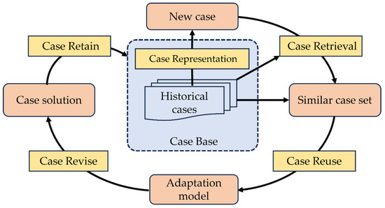
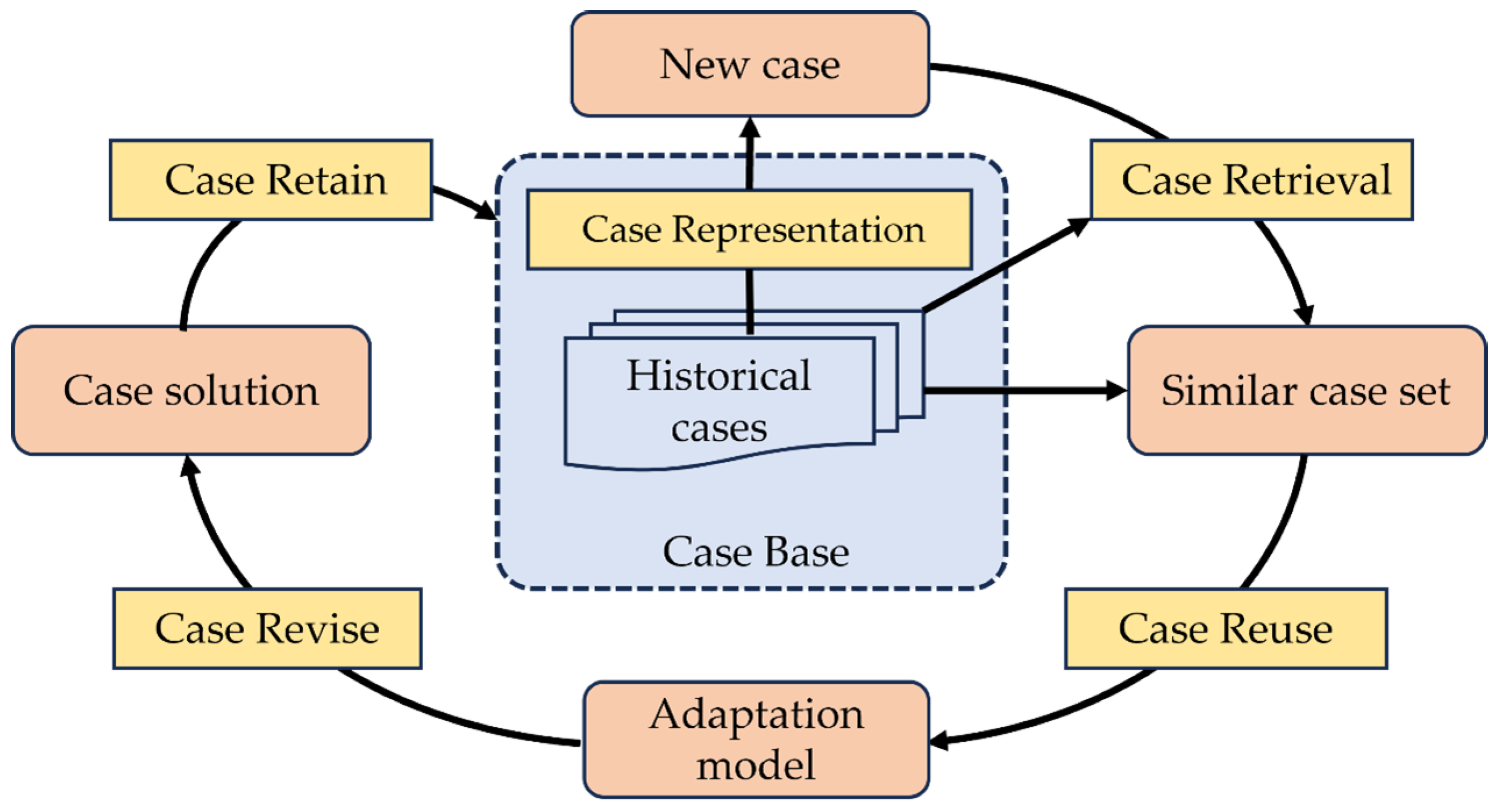
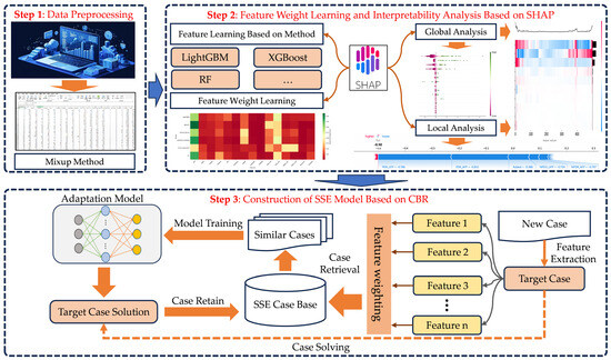
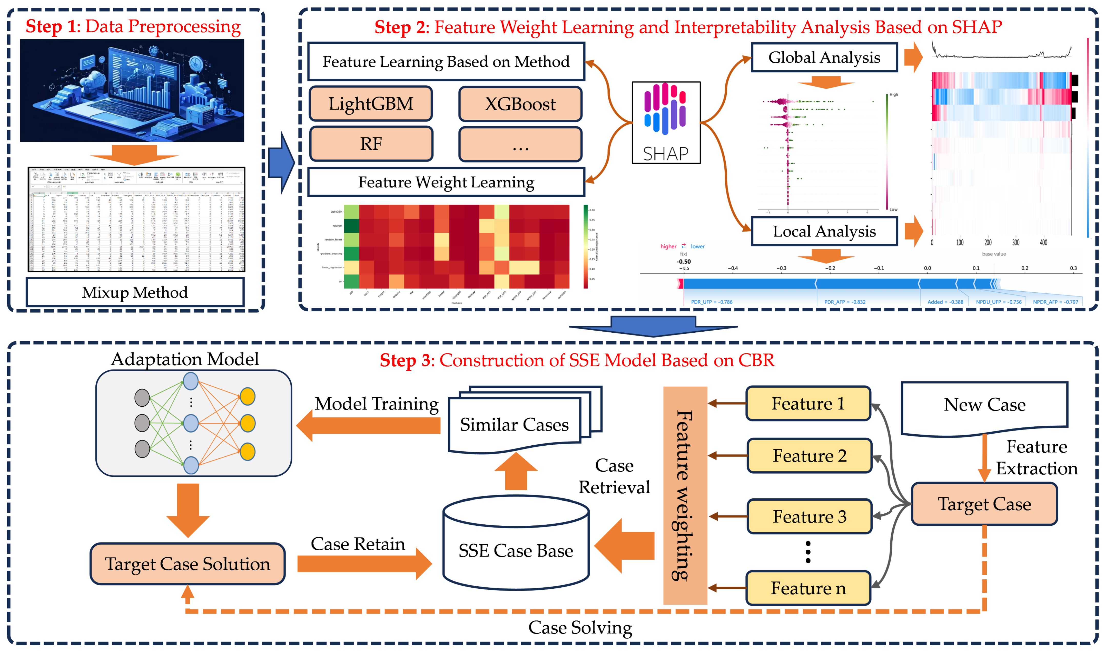
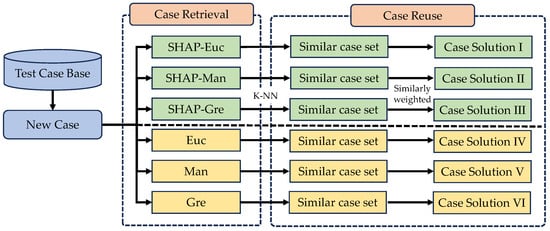
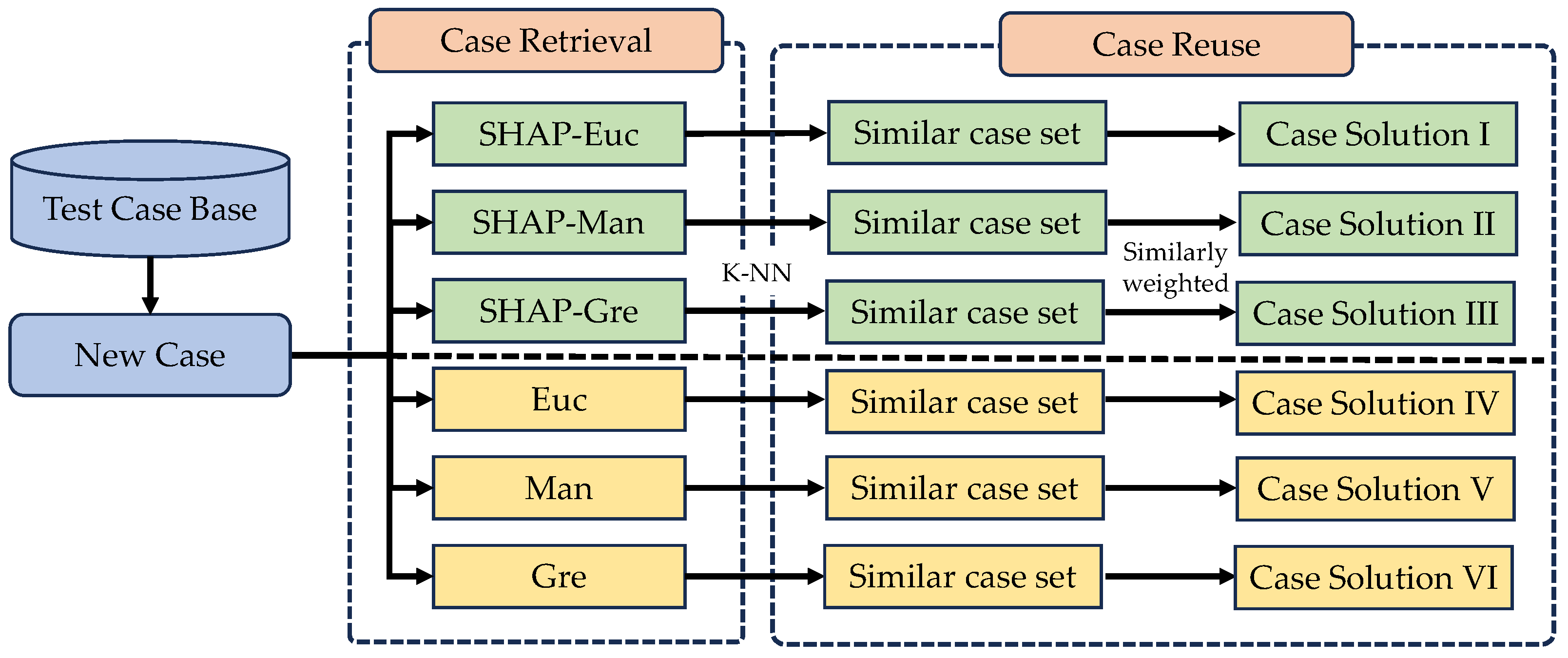
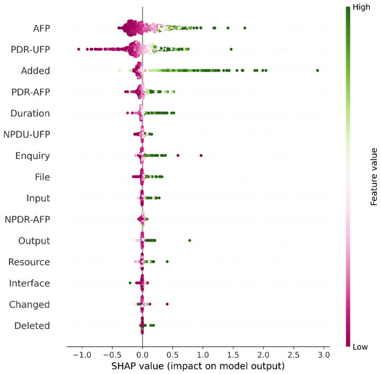
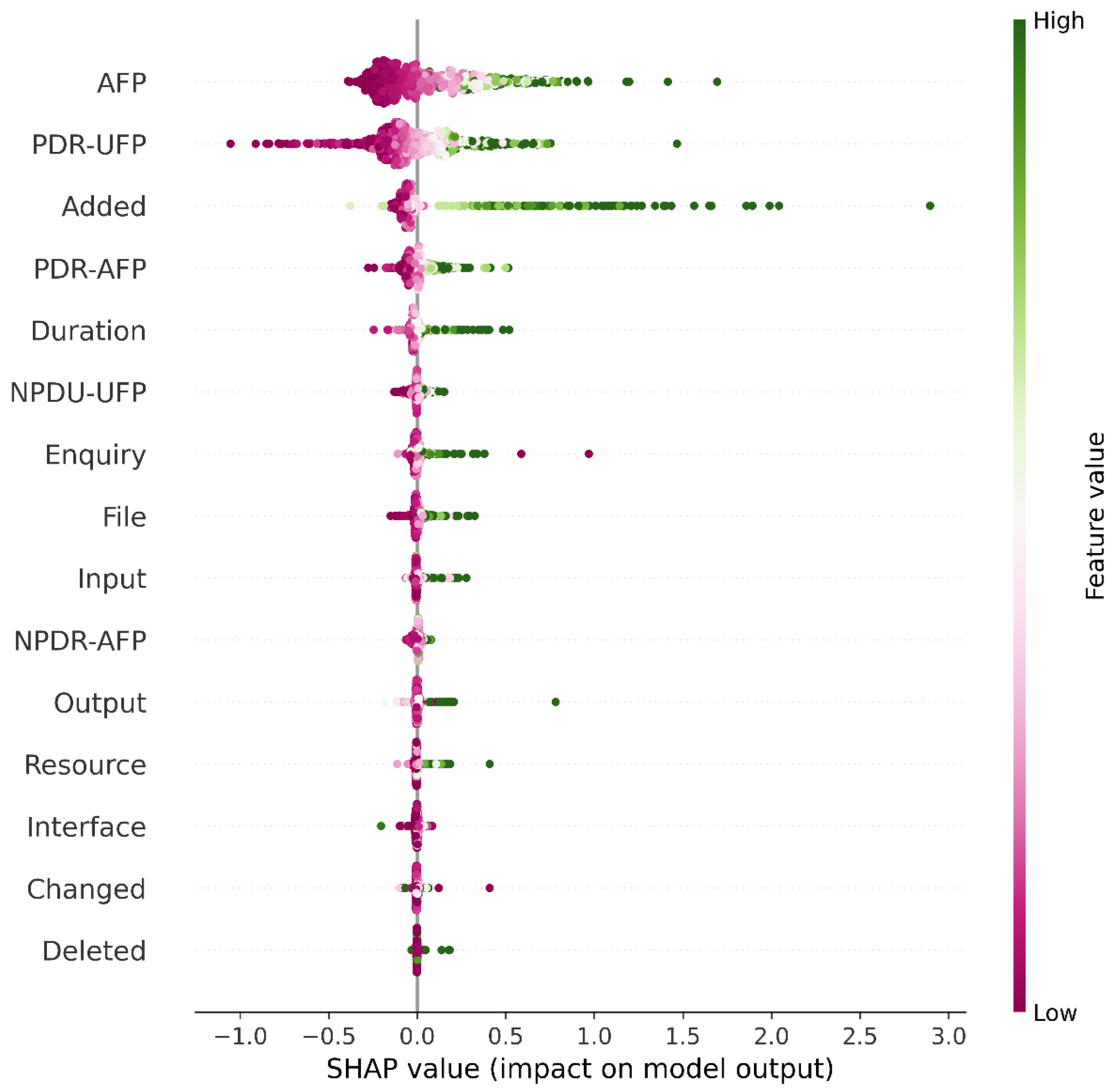
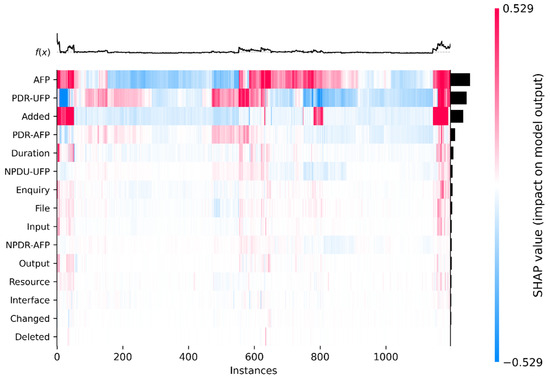
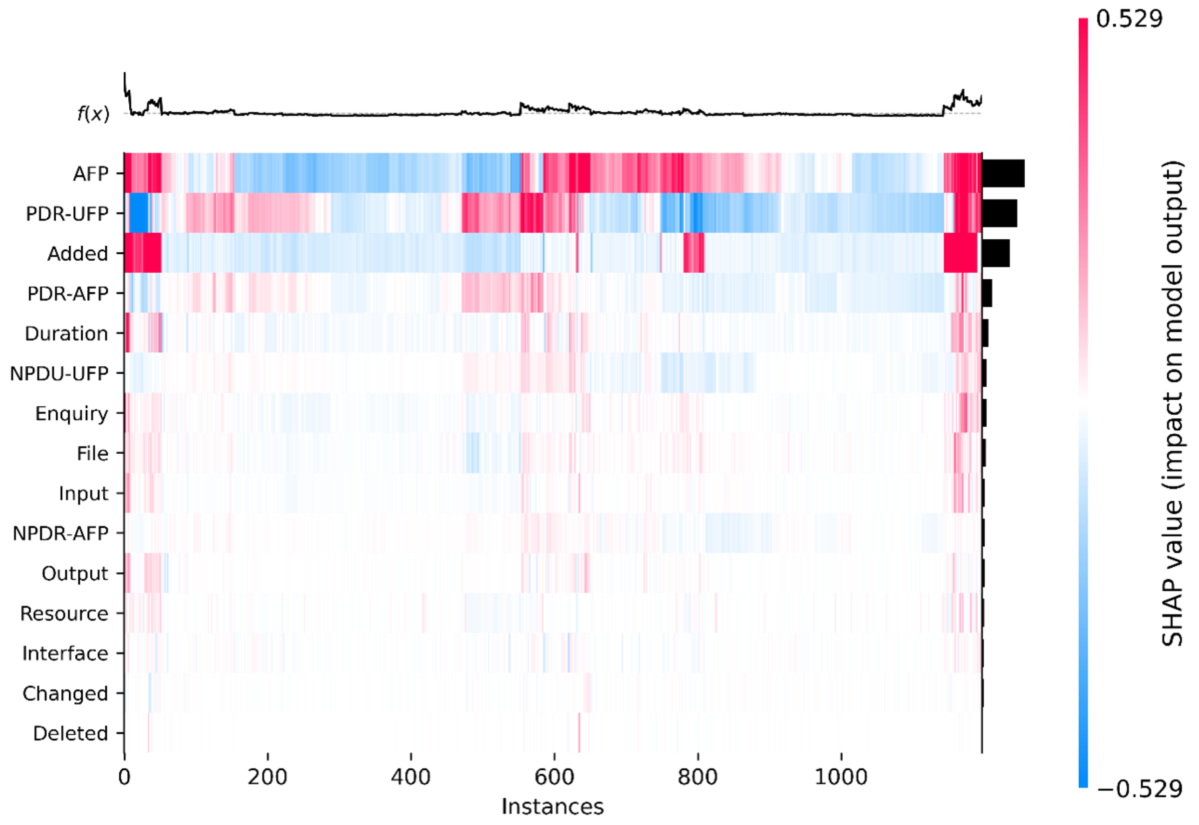
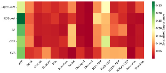
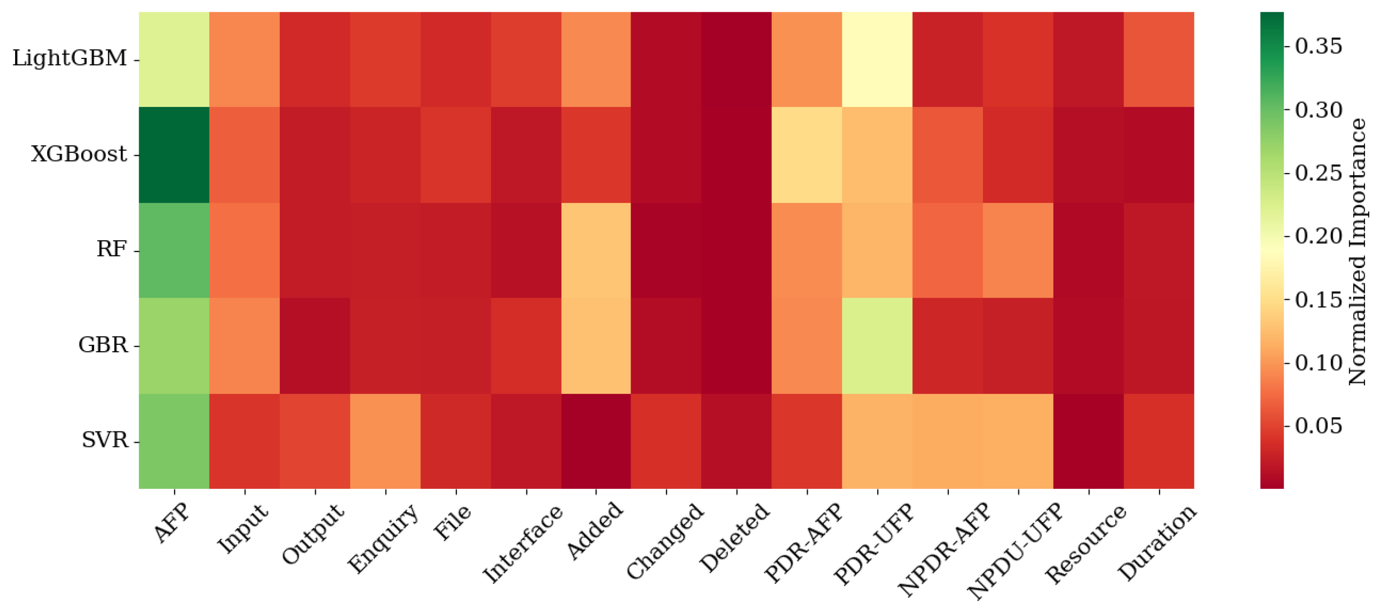
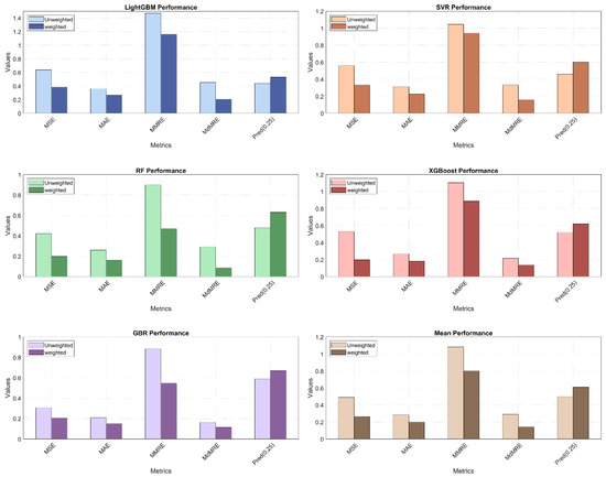
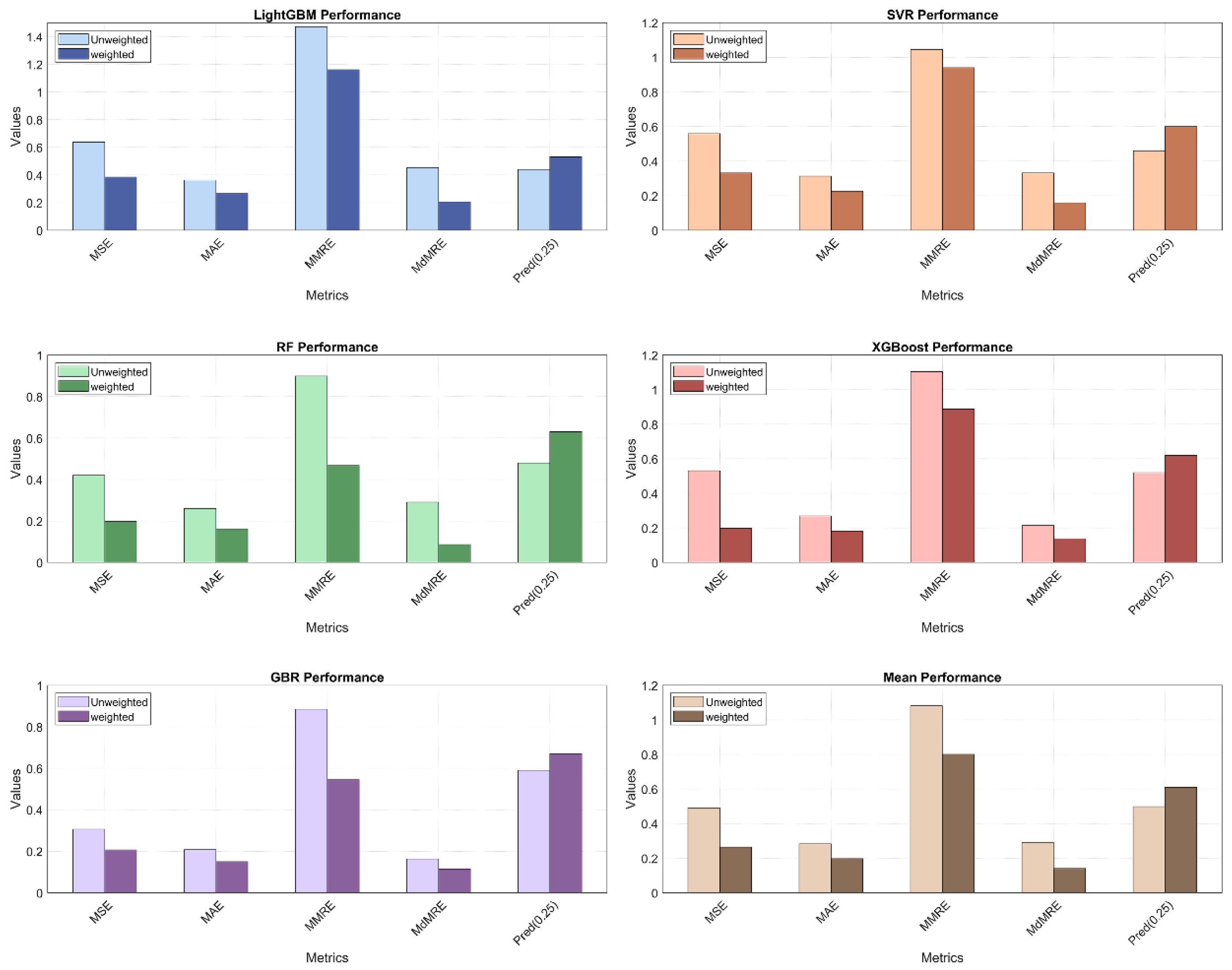
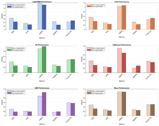
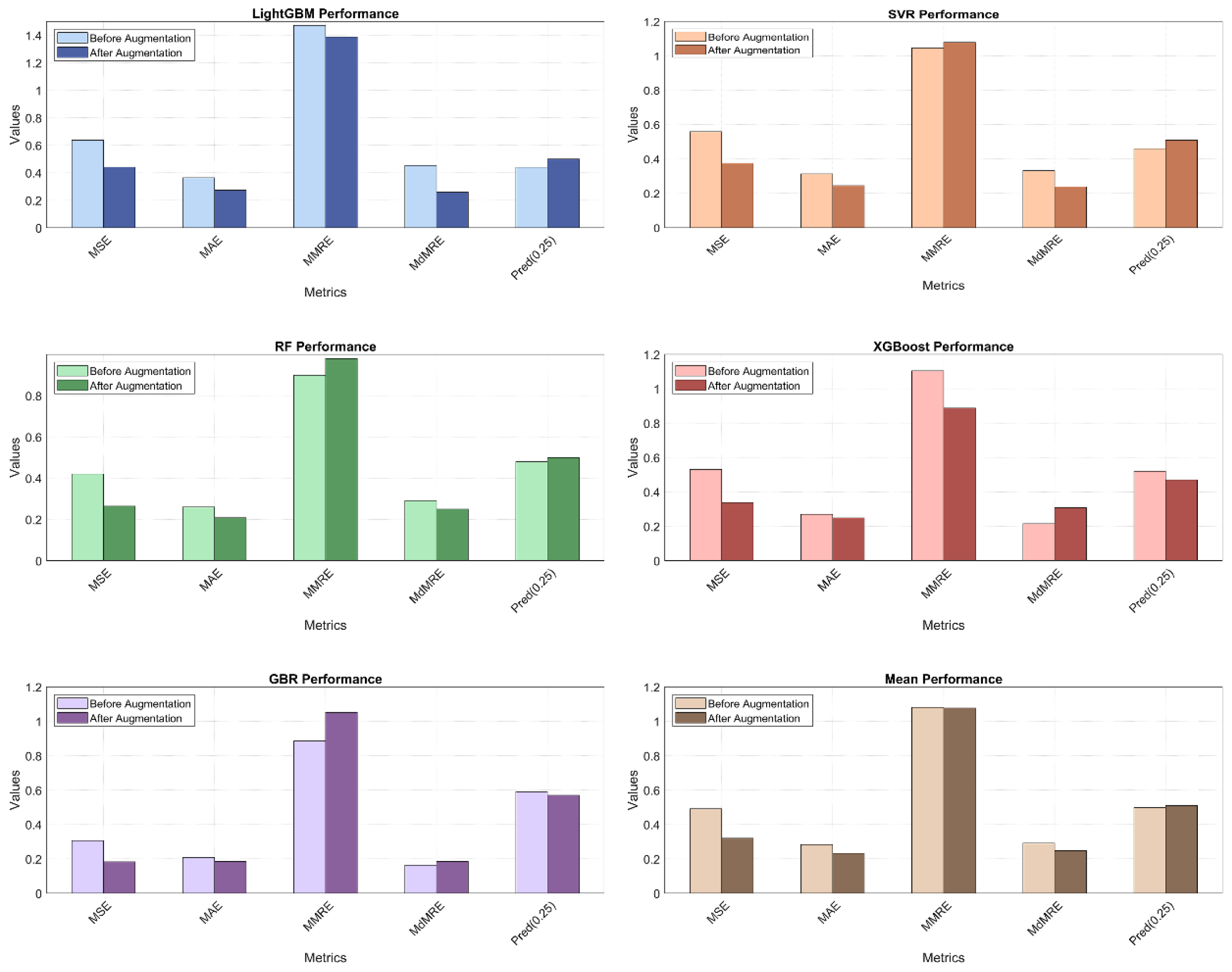
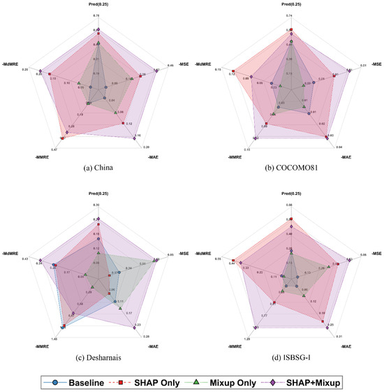
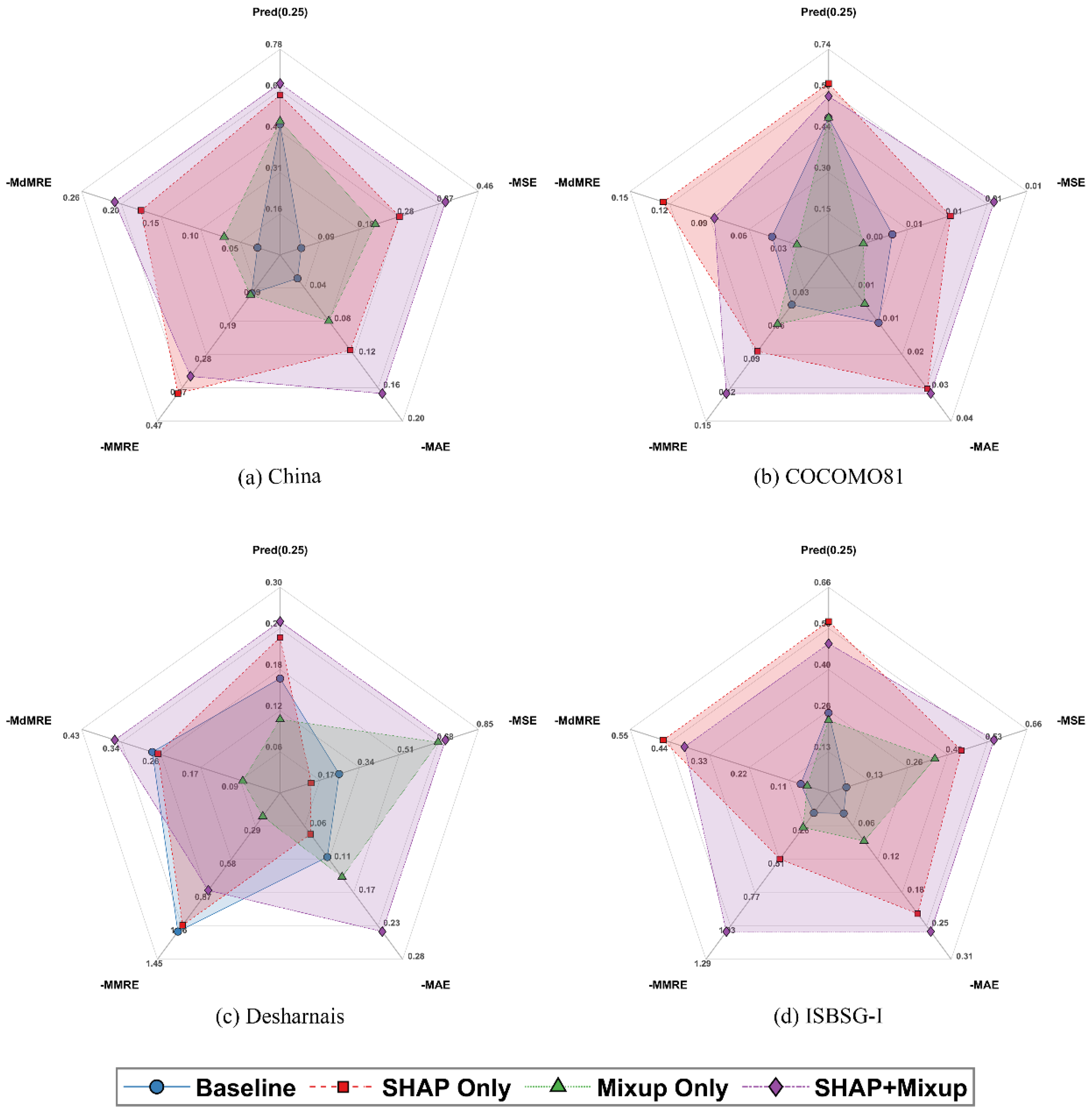

Disclaimer/Publisher’s Note: The statements, opinions and data contained in all publications are solely those of the individual author(s) and contributor(s) and not of MDPI and/or the editor(s). MDPI and/or the editor(s) disclaim responsibility for any injury to people or property resulting from any ideas, methods, instructions or products referred to in the content. |
© 2026 by the authors. Licensee MDPI, Basel, Switzerland. This article is an open access article distributed under the terms and conditions of the Creative Commons Attribution (CC BY) license.