


Abstract
AI infrastructure is entering a constraint-dominated regime in which power access, cooling, water conditions, reliability, and financing jointly shape cost, sustainability, and operational risk. Yet the metrics used to evaluate these systems remain fragmented across facility engineering, compute/workload performance, and economic or risk analysis, with definitions that often sit at different layers and under different boundaries. This fragmentation weakens cross-layer reasoning and makes decision-traceable trade-off analysis difficult. This paper proposes a structured, decision-oriented measurement architecture for AI infrastructure metrics. The framework combines a 6 × 3 taxonomy, which organizes metrics across six layers and three semantic domains, with a procedural workflow built around a problem card, variable registry, minimality gate record, activated-cell map, boundary log, metric ledger, and a results sheet with case-pack manifest. Within this protocol, the Metric Propagation Graph is used as a case-specific dependency representation for tracing decision-facing metrics back to minimal boundary-consistent inputs. It is introduced as a traceability layer within the framework rather than as a stand-alone graph-theoretic method. The paper is illustrated through one fully worked case and one scoped portability illustration. The first is a fully worked large-load planning case for the Northern Virginia data-center corridor within PJM’s Dominion zone, showing that a boundary-consistent integrated metric can reverse the ranking obtained under a simpler screening view. The second is a scoped portability illustration for hourly matching under dual Scope 2 boundaries. Its purpose is not to provide a second full empirical validation, but to show how the same dossier logic, boundary discipline, and traceable metric construction transfer to a distinct decision setting.
1. Introduction
AI infrastructure has reached a point at which measurement is no longer a secondary reporting function. It has become part of the operating core. The scale of electricity demand, carbon exposure, water dependence, and grid interaction associated with modern data centers has already made infrastructure evaluation a first-order planning problem rather than a downstream technical detail [1,2,3]. At the same time, the metric environment has become increasingly crowded. Reviews of data-center efficiency practice now document a wide and expanding landscape of operational indicators, many of which were introduced to solve immediate management problems rather than to support a stable, cross-layer decision system [4]. This is also how the largest AI infrastructure operators increasingly work in practice. Bottleneck detection, utilization control, thermal management, service monitoring, and cost governance all rely on large and evolving collections of metrics. Yet the metric system itself often remains under-structured. Many indicators enter operational use without a clear account of what they measure, where they belong, or how they relate to other metrics already in circulation. New measures appear quickly, older ones are revised or reinterpreted, and the evolution of these metrics is rarely logged in a way that makes later comparison, revision, or audit straightforward. The result is a measurement environment that is rich in signals but weak in structure.
This matters because AI infrastructure decisions are increasingly framed as optimization problems. Some are local, such as workload placement, communication scheduling, cooling control, or accelerator utilization. Others are system-level, such as sitting large loads, designing procurement portfolios, comparing deployment architectures, or balancing cost, reliability, and sustainability across teams. Existing benchmarks and systems traditions already provide powerful tools for parts of this space, including training and inference benchmarking, distributed execution efficiency, and environmentally aware model development [5,6,7,8]. Economic and infrastructure studies similarly show that cost, pricing, cooling, and resilience decisions cannot be understood at a single layer of the stack. Total-cost logic, facility pricing structures, cooling-grid coupling, resilience design, electricity-price pass-through, and levelized economic comparison all influence what a system actually costs and how it should be managed [9,10,11,12,13]. In principle, these problems require a declared decision boundary, a justified variable set, and a transparent link between engineering states and economic outcomes. In practice, the setup is still often fragmented. Relevant metrics are scattered across technical sectors and organizational teams, data interfaces are uneven, variables are assembled ad hoc, and problem definition itself can take substantial time before a model is even ready to run. Once the setup changes, objectives, variables, and constraints are difficult to revise in a controlled way. Tracing why a metric entered the system, how it was transformed, or whether an integrated result remains auditable and valid is often harder than producing the result in the first place.
The underlying difficulty is structural rather than terminological. AI infrastructure operates as a coupled multi-layer system in which power, cooling, hardware behavior, workload execution, service delivery, and lifecycle value propagate across boundaries rather than staying within isolated subsystems. This is why narrowly local optimization often fails to settle broader planning questions. The literature contains many useful examples of subsystem optimization and cost-aware engineering, including work on minimizing cooling and server power costs, tracing hidden deployment costs, understanding the role of component-level power consumption, and linking power-sector carbon policies to economic outcomes [14,15,16,17]. But these contributions do not by themselves provide a common architecture for deciding which metrics should enter a given planning problem, how they should be placed across system layers, or under what accounting boundaries they can be validly combined. A locally meaningful improvement can shift burden elsewhere, alter the relevant denominator of comparison, or weaken the interpretation of a cost or sustainability claim once viewed at the system level. What appears to be a measurement problem is therefore also a planning and governance problem.
The field does not suffer from a shortage of metrics. It suffers from the absence of a disciplined structure for using them together. Existing indicators remain meaningful within their native technical or operational boundaries, but three practical failures occur once they are used for integrated planning. First, incompatibility weakens attribution and traceability. A facility-side indicator can reveal overhead, but not whether that overhead is driven by thermal design, workload behavior, hardware utilization, or external grid conditions. Second, overlap and boundary ambiguity create room for both double-counting and silent omission. Measures that appear comparable often rely on different objects, denominators, or semantic boundaries. Third, subsystem-optimal KPI use can distort system-level decisions. A metric may improve within one layer while worsening reliability exposure, carbon-adjusted cost, or delivered-service value elsewhere. Supplementary online Appendix A provides an extended cross-family landscape summary. The narrower point for the present paper is that current practice still lacks a coherent architecture for placing metrics, aligning meanings, declaring boundaries, and composing decision-facing quantities without hidden inconsistency.
The contribution sought here is therefore different from that of a conventional review, a standard techno-economic case study, a generic multi-criteria ranking exercise, or an operational KPI dashboard. Review and survey studies are valuable for organizing prior metrics and practices, but they do not by themselves specify how metrics should be placed, filtered, and composed under an explicit decision boundary. Techno-economic studies can deliver cost and performance comparisons for a particular application, but they usually take the metric set, accounting boundary, and case scope as part of the case setup. Multi-criteria frameworks can rank alternatives once a metric portfolio is already given, but they typically do not address whether that portfolio is semantically aligned, minimally sufficient, or traceable to declared upstream inputs. KPI dashboards improve monitoring and visibility, but they do not provide a closure rule for building a small decision-facing evaluator. The present paper contributes to that earlier architectural layer. It develops a structured measurement architecture for AI infrastructure decisions in which metric placement, boundary declaration, minimal case closure, and traceable integrated-metric construction are treated as explicit parts of the problem rather than as background assumptions.
This paper addresses that gap by proposing a structured, decision-oriented measurement architecture for AI infrastructure metrics. The contribution is threefold. First, a cross-layer 6 × 3 taxonomy locates heterogeneous metrics by system layer and semantic domain, providing a common coordinate system without erasing native measurement meanings. Second, a procedural workflow translates a planning question into a documented decision dossier through a problem card, variable registry, minimality gate record, activated-cell map, boundary log, metric ledger, and results sheet/case-pack manifest. Third, a case-specific Metric Propagation Graph is introduced as a traceability layer within the framework. Its purpose is to record first-order dependency paths from decision-facing metrics to upstream primitives, proxies, and boundary-conditioned transformations, and to make closure, omission, and potential redundancy readable under declared boundaries. The architecture is then demonstrated in two intentionally asymmetric ways: one fully worked case-based implementation and one scoped portability illustration. The first shows how framework-guided metric synthesis can change planning interpretation once service boundaries, carbon exposure, and reliability penalties are made explicit. The second shows how the same dossier logic can be transferred to a distinct boundary-intensive setting without being presented as a second full empirical validation.
The remainder of the paper is organized as follows. Section 2 develops the static measurement architecture through the 6 × 3 taxonomy. Section 3 formalizes the decision-dossier workflow and the MPG traceability logic. Section 4 presents one fully worked case-based implementation and one scoped portability illustration, and Section 5 concludes.
2. Unified Measurement Architecture
The central problem is not the lack of metrics, but the lack of a common structure for using them together in planning, comparison, and metric construction. Existing indicators remain meaningful within their native technical or operational boundaries, yet they rarely align automatically when a decision problem spans facility constraints, compute delivery, service outcomes, and lifecycle valuation. A unified architecture is therefore needed before procedural metric selection or synthesis can proceed. Without such an architecture, integrated evaluation remains vulnerable to boundary drift, semantic mismatch, and hidden double counting.
This section develops static architecture. It organizes heterogeneous AI-infrastructure metrics without forcing them into a single unit system or a single optimization language. Two orthogonal axes are introduced. The first defines three meta-level metric domains that capture the main measurement semantics. The second defines a six-layer system stack that fixes operational boundaries from external grid conditions to the delivered AI service. Together, these axes form a 6 × 3 taxonomy that supports disciplined metric placement, boundary-consistent comparison, and the later construction of integrated decision metrics. The taxonomy should therefore be read not as a convenience classification, but as the structured synthesis layer of the framework: it translates a fragmented metric landscape into a stable coordinate system for later case construction and boundary-consistent comparison.
2.1. Three Meta-Level Metric Domains
The first axis of the architecture is semantic. AI-infrastructure metrics are grouped into three mutually exclusive meta-domains according to what they directly measure and the unit system they inhabit. The three domains are physical facility performance and efficiency, compute and workload efficiency, and lifecycle economics and reliability risk.
These domains define the horizontal structure of the 6 × 3 taxonomy. Primitive metrics map to exactly one domain based on their primary object and native units. Composite decision metrics may draw inputs from more than one domain, but they are assigned to the domain of the decision objective they operationalize. Cross-domain dependence is therefore not suppressed. It remains explicit through recorded dependency paths and becomes central once integrated metrics are constructed later in the paper.
2.1.1. Domain 1. Physical Facility Performance and Efficiency
The first domain covers the physical overheads and resource-conversion conditions that determine how electricity, cooling capacity, water, and thermal headroom are translated into IT-usable operating conditions. Its core measures are the xUE family and related facility indicators. ISO/IEC 30134 provides formal definitions for widely used measures such as PUE, WUE, CUE, and ERE, while ASHRAE thermal guidance defines the operating envelopes that shape airflow management, heat rejection, economization, and power-train losses [18,19]. These constructs are also reflected in hyperscaler reporting and operational disclosure practices, including public materials from Google and Meta [20,21,22,23]. Metrics in this domain are expressed in physical ratios and resource intensities such as kWh/kWh, L/kWh, and gCO2/kWh. They do not measure computing output or monetary value directly, but they strongly affect both. In practice, they shape recurring operating costs through electricity and water demand, influence facility-side capital requirements through cooling and power infrastructure, and determine how strongly environmental and carbon conditions enter downstream decision metrics.
2.1.2. Domain 2. Compute and Workload Efficiency
The second domain covers the transformation of IT power and installed hardware into effective computational output. It includes both device-level efficiency and workload-level execution behavior. The domain draws on high-performance computing, accelerator benchmarking, and ML systems evaluation. Green500 established FLOPs/W as a canonical device-efficiency benchmark, while modern accelerator platforms and system stacks now report metrics such as tokens per joule, joules per training step, scaling efficiency, and communication overhead under distributed execution [24,25,26]. Benchmarking efforts such as MLPerf extend the boundary from hardware capability to end-to-end workload behavior by reporting time-to-convergence, latency, and throughput under standardized execution conditions [27]. Metrics in this domain are expressed in computational units such as FLOPs, operations per second, joules per operation, batches per second, or sequences per second. Their role is to capture how much useful compute is delivered per unit of IT power and installed capacity. Their economic importance is substantial, but indirect. They influence cost per token, cost per request, training duration, and the rate at which accelerator capital can be productively amortized, even though the metrics themselves remain computational rather than monetary.
2.1.3. Domain 3. Lifecycle Economics and Reliability Risk
This domain covers valuation, lifecycle accounting, and operational risk. It is the domain in which technical states are translated into decision-native economic terms. Total cost of ownership frameworks decompose capital expenditure, operating expenditure, depreciation, staffing, interconnect cost, energy procurement, and refresh cycles into lifecycle cost objects suitable for planning and comparison [28,29]. Energy economics contributes levelized formulations such as LCOE, while newer work extends this logic toward cost normalization for AI infrastructure and delivered AI service [30,31]. Reliability and continuity measures, including MTBF, MTTR, and service-oriented constructs drawn from site reliability engineering, translate failure behavior into downtime loss, redundancy burden, and penalty exposure [32]. Recent policy and strategy discussions also increasingly frame reliability, energy, and lifecycle economics as linked infrastructure concerns rather than separate engineering topics [33]. Metrics in this domain are therefore expressed in monetary quantities, probabilities, and risk measures such as USD per year, depreciation schedules, failure distributions, or expected loss. They do not measure physical conversion or computational transformation directly. Instead, they provide the valuation and risk semantics under which infrastructure decisions are ultimately compared and justified.
2.1.4. Rationale and Scope
The three-domain decomposition is semantic and unit-consistent rather than organizational. Each primitive metric is assigned to a unique domain based on what it directly measures and the units in which it is natively expressed. Apparent cross-domain cases usually arise only when a decision metric is composite by design. Carbon-adjusted cost is one example. It combines a physical input, such as carbon intensity, with a valuation rule, but the resulting metric still belongs to the economic and risk domain because its decision object is monetary comparison rather than physical accounting. The same logic applies more broadly: cross-domain dependence is allowed, but semantic placement remains unique at the primitive level. This distinction is important because it prevents the taxonomy from collapsing into a convenience-based classification in which similar-sounding metrics are grouped together despite measuring different objects. The broader AI-infrastructure metric dictionary is provided in Supplementary Appendix A, with additional supporting materials reported in Supplementary Appendices B and C. A formal justification of minimality and completeness is provided in Supplementary Appendix D.
The three meta-domains establish semantic meaning, but they do not by themselves identify where in the system stack a metric is defined or where its operational boundary applies. That second task requires a vertical decomposition of the infrastructure itself. The next subsection therefore introduces a six-layer architecture that fixes operational interfaces from external grid exposure to delivered AI service and makes propagation channels across the stack explicit.
2.2. The Six-Layer Architecture of AI Infrastructure
AI infrastructure is represented here as a six-layer stack running from external grid conditions to delivered AI service. The purpose of this decomposition is not to mirror a single firm’s internal org chart, but to recover the operational structure that repeatedly appears in large-scale AI infrastructure planning. Across leading operators, decisions are made across a sequence of linked interfaces: electricity is sourced from the grid environment, converted into facility-usable power, transformed by compute hardware into raw computational capacity, coordinated through cluster networking, translated by ML systems into executable training or inference throughput, and finally realized as service delivered to downstream users or applications. These interfaces define the foundations of the six layers. Each layer is therefore specified by its operational scope, its boundary with adjacent layers, and the main economic channel through which cost, reliability, and performance effects propagate upward or downward through the system.
- (1)
- Layer 1—Grid and Sustainability. This layer reflects the external operating environment, including electricity availability, price signals, fuel mix, temporal carbon intensity, and policy or procurement constraints. The interface to Layer 2 is electricity delivered at the point of interconnection, along with its associated “quality” in price, emissions, and outage or curtailment risk at the relevant region and time [34,35,36,37]. Economically, Layer 1 sets baseline exposure for OpEx and establishes carbon- and reliability-linked liabilities that downstream layers inherit unless boundary-adjusted.
- (2)
- Layer 2—Facility. This layer covers non-IT infrastructure that determines how delivered electricity becomes IT-usable power. It includes power distribution and conversion, UPS losses, cooling systems, and auxiliary loads. The interface is the conversion from grid-supplied electricity to IT-deliverable power under thermal and electrical constraints, which depend on facility design and operating regime [19]. Economically, Layer 2 drives recurring overhead beyond IT load and creates capacity bottlenecks, such as heat-rejection limits, which raise the shadow price of additional compute.
- (3)
- Layer 3—Compute Hardware. This layer comprises accelerators, CPUs, memory, and storage that transform IT power into raw compute capability. Its interface upward is the mapping from IT power and installed hardware to usable compute capacity, shaped by utilization, heterogeneity, and reliability behavior [25,26]. Economically, Layer 3 is the main driver of capital intensity and performance per dollar. It also determines how much energy becomes useful computing rather than idle, throttled, or redundancy-provisioned capacity.
- (4)
- Layer 4—Cluster Networking and Interconnect. It captures the fabric that enables distributed training and serving at scale. It includes topology, bandwidth, contention, and tail behavior. The interface is the translation from node-level compute potential to cluster-level effective throughput after accounting for synchronization and communication costs. Economically, it governs the gap between purchased capacity and realized time-to-solution, shaping computing productivity and overprovisioning.
- (5)
- Layer 5—ML Runtime, Workload Execution, and Resilience (Fault-Tolerance). It represents the software and workflow mechanisms that determine effective utilization, including scheduling, batching, checkpointing, fault tolerance, and algorithmic efficiency. The interface is a software-driven multiplier that maps cluster capability to delivered workload progress under stochastic failures and performance variability, consistent with workload-level benchmarking semantics [27,28]. Economically, it turns variability into cost through delays, wasted energy, and missed objectives.
- (6)
- Layer 6—Service, Operations, and Economic Outcomes. This layer describes what is ultimately delivered and valued. It includes throughput and latency, availability, compliance performance, and lifecycle cost. Typical decision-native quantities include time-to-solution, SLA/SLO attainment, downtime exposure, TCO, and cost normalizations that incorporate energy and carbon valuations depending on context [28,29,30,31]. Layer 6 inherits runtime-induced variability from Layer 5 but evaluates it at the service boundary in terms of compliance and loss. Economically, Layer 6 aggregates the consequences of the lower layers into objective functions and constraints used in siting, procurement, capacity planning, and policy assessment.
2.3. The Unified 6 × 3 Metrics Taxonomy
The taxonomy organizes metrics by layer, with ℓ ∈ {1, …, 6}, and by domain, with d ∈ {Physical, Compute/Workload, Economic/Risk}. The layer index fixes the operational boundary across grid, facility, hardware, interconnect, runtime, and service or economic outcomes. The domain index identifies what the metric primarily measures, if it is a resource or physics constraint, a computational transformation, or a valuation and risk outcome. Table 1 reports the coverage map used in this paper.
Table 1.
Taxonomy Coverage Map—Three Meta-Domains and Six Infrastructure Layers.
How to read the taxonomy. Table 1 is a placement map rather than a checklist of all metrics that must appear in every case. The row identifies the operational boundary at which a metric is natively defined, while the column identifies its primary semantic meaning. Primitive metrics are placed in one cell only. Integrated decision metrics may draw on inputs from multiple cells, but they are assigned to the cell corresponding to the decision object they operationalize. This distinction is important because it keeps semantic placement separate from cross-layer dependence, which is handled later through the dossier workflow and the MPG trace.
The taxonomy distinguishes reliability by where it is measured and what it measures. At Layer 5, reliability is treated as execution resilience: it affects delivered progress through runtime mechanisms such as checkpointing and retry overhead, and is expressed as slowdown, wasted work, or completion-time dispersion. At Layer 6, reliability is treated as service assurance and monetized exposure: it is measured through SLIs/SLOs/SLAs and valued through downtime loss, penalty exposure, or risk measures. This separation prevents double-counting when a decision metric combines runtime overhead with service-level consequences.
The coordinate system is designed to prevent common boundary errors. One example is comparing throughput metrics that embed different assumptions about facility overhead. Another is comparing cost metrics that silently differ in carbon pricing or reliability valuation [38]. The taxonomy also clarifies where propagation must be accounted for. Physical feasibility and overhead in Layers 1–2 constrain effective compute in Layers 3–5, and these constraints ultimately shape decision outcomes in Layer 6. When such couplings are ignored, conclusions can be directionally wrong even if each subsystem KPI is locally correct.
A simple reading example clarifies the intended use. PUE is placed in Layer 2, Domain 1, because it measures facility-side overhead under a physical resource boundary. FLOPs/W is placed in Layer 3, Domain 2, because it measures the transformation of IT power and hardware into usable compute. By contrast, CRCC is placed in Layer 6, Domain 3, even though it depends on upstream physical and workload variables, because its decision object is a valued service-level comparison. The purpose of the taxonomy is therefore not to collapse unlike metrics into one unit system, but to show where each metric natively belongs and which cross-cell dependencies must later be made explicit.
A practical implication is domain complementarity. Physical-domain metrics define feasibility frontiers and overheads imposed by energy and cooling constraints. Compute and workload metrics capture how effectively IT power and hardware translate into realized workload progress. Economic and reliability metrics translate technical states into valuation and risk. No single domain is sufficient on its own. Physical metrics can overstate capability if performance losses and resilience overhead are omitted. Compute and workload metrics can overstate efficiency if facility and grid constraints are ignored or left unadjusted. The taxonomy highlights cross-cell failure modes where decision mistakes are most likely, especially when Layer-6 outcomes depend on joint variation in upstream physical constraints in Layers 1–2, hardware and interconnect bottlenecks in Layers 3–4, and runtime resilience behavior in Layer 5 [39].
2.4. Operational Metric-Selection Playbook
The taxonomy supports a first-pass discipline for metric selection before formal case construction begins. In practice, three questions should be answered at this stage. First, what is the decision-native target, usually a Layer-6 metric expressed per unit of delivered service or delivered compute? Second, which upstream layers contain the binding constraints or dominant drivers for that target? Third, which minimal upstream quantities must remain active for the target to be interpreted without semantic drift or hidden double-counting? At this stage, the taxonomy functions as a structured reading guide rather than a complete case protocol. It clarifies where metrics belong, which cross-layer dependencies are likely to matter, and where integrated metrics may be needed. Section 3 then turns this preliminary discipline into an explicit decision-dossier workflow with registry, minimality gate, boundary log, metric ledger, and results sheet artifacts.
3. A Procedural Framework for Metric Selection and Decision Dossier Construction
The 6 × 3 taxonomy is intentionally static. It defines where metrics belong in the system stack and clarifies their semantic boundaries, but it does not by itself determine which upstream quantities materially drive a downstream decision under a stated price, carbon, or service boundary. Applied planning and optimization-oriented case construction therefore require a second layer. That layer must translate a decision question into a minimal, boundary-consistent metric system that can be executed, audited, and reused across cases.
This section develops that procedural layer. The framework is organized around two primary elements and one supporting representation layer. The taxonomy provides the semantic coordinate system. The decision dossier provides the procedural workflow through which a case is scoped, closed, logged, and archived. The Metric Propagation Graph (MPG) supports this by recording first-order dependency paths from a decision-facing target to the smallest upstream set of declared primitives, proxies, and boundary-conditioned transformations needed for interpretation. The decision dossier records the artifacts that make a case reproducible, comparable, and auditable. The output is not a generic variable catalogue, but a minimal metric system closed under explicit boundary choices and documented data interfaces. Minimality is understood operationally. A case is considered closed when its target and binding constraints can be computed from declared primitives, declared proxies, and logged accounting rules, without uncontrolled proliferation of secondary quantities.
3.1. Framework Logic and Dossier Objects
The framework treats metric selection as a feasibility and closure problem that precedes formal model construction. Optimization problems often become fragile because variables are introduced incrementally, often in response to data convenience or local intuition, rather than through an explicit accounting of what is required to close the decision system. The present framework reverses that order. The starting point is a decision-native target together with its service requirement and sustainability or reporting boundary. From there, the framework identifies the smallest set of quantities required to support a valid comparison under the stated interpretation.
The following major decision-dossier artifacts carry this logic. After the problem card establishes the decision setting, the first operational artifact is the variable registry, which consolidates candidate variables into a single auditable table with taxonomy placement, role classification, inclusion priority, and data support. Based on the variable registry, a minimality gate is deduced regarding feasibility and problem refinement. The second is the activated-cell map, which marks the subset of taxonomy cells required for closure and assigns one primary variable to each active cell. The third is the boundary log, which fixes the price, carbon, and accounting conventions under which integrated metrics will be interpreted. The fourth is the metric ledger, which records composite decision metrics as traceable recipes rather than opaque outputs. The fifth is the results sheet and case-pack manifest, which summarize the evaluator, note limitations, and archive the case in a reusable form. The MPG supports all five objects by preserving dependency paths from target metric to upstream primitives. It is used here as a measurement and traceability scaffold, not as a causal graph or a dynamical systems model.
Formally, each case-specific MPG can be represented as a directed typed dependency graph . Nodes record declared objects in the case dossier, including primitives, proxies, fixed parameters, decision variables, intermediate quantities, boundary tags, and integrated decision metrics. Directed edges record first-order dependency relations such as physical transformation, accounting aggregation, normalization, valuation, or boundary-conditioning. The MPG is admissible only when every target metric in the case can be traced along directed paths to declared upstream inputs under the logged accounting boundary. In this paper, the graph is used as a readable closure and traceability device rather than as an optimization algorithm or an autonomous graph-construction procedure.
To keep the role of the MPG precise, Table 2 introduces only the minimal node and edge classes needed for case closure and metric provenance in the present framework. The purpose is not to define a stand-alone graph-theoretic language, but to make dependency tracing readable and reproducible within the decision dossier. In other words, the MPG is used here as a compact traceability layer attached to case construction, not as a causal graph, a universal ontology, or an autonomous optimization routine.
Table 2.
Minimal MPG Schema Used in This Framework.
Two design principles govern the framework throughout. The first is one-primary-variable-per-activated-cell. This rule keeps the system readable and prevents the case from expanding into a broad variable inventory that is hard to calibrate or audit. The second is boundary-first integration. Cross-layer metrics often change meaning when the electricity boundary shifts from wholesale nodal prices to contract settlement values, or when emissions are evaluated under different reporting conventions. Boundary definitions are therefore treated as formal inputs rather than explanatory footnotes. Integrated metrics are reported only after the relevant price, carbon, and accounting rules have been fixed in the dossier.
3.2. Operational Protocol for Traceable Case Execution
Figure 1 summarizes the protocol in simplified form. It should be read as an execution sequence for decision-dossier construction rather than as a generic conceptual diagram. The steps are ordered because semantic placement, feasibility, minimality, and boundary declaration must be fixed before an integrated metric can be reported. Each step produces a readable artifact that can be checked on its own and archived for later reuse. In this sense, the protocol does not merely organize model inputs. It produces a small, auditable case object.
Figure 1.
Operational Protocol for Traceable Case Execution. The figure is a procedural overview rather than an algorithmic flowchart. Blue arrows indicate the normal sequential workflow, while the red dashed arrow indicates the failure path from the minimality gate, which requires scope reduction and re-logging. The left-side labels group the workflow into scoping, gateway, integrity, and synthesis phases. Each step produces a readable artifact used to support case closure, boundary logging, and integrated-metric traceability.
Step 1. Problem card and target definition. Each case begins with a short problem card. The card records the decision actor, planning horizon, service requirement, and sustainability or compliance boundary relevant to interpretation. It also fixes the target metric, usually a Layer-6 economic or risk metric expressed per unit of delivered service or delivered compute. A brief grounding statement ties the case to a recognizable industry or policy context so that the exercise is not read as a purely illustrative abstraction.
Step 2. Variable registry with priority and availability. Candidate variables are then consolidated into a single registry that also serves as the case feasibility ledger. The registry records each variable’s taxonomy cell, variable class, and primary role in the evaluator as target, constraint component, driver, state, or derived quantity. Priority is recorded as Must, Should, or Optional, depending on whether the variable is necessary for dependency closure of the target and binding constraints under the stated boundary conditions. Data support is recorded as Direct, Proxy, or None, together with the relevant public interface or data source. In the revised manuscript, Table 3 defines the registry schema used throughout the case demonstrations. Its purpose is not clerical. It makes explicit which quantities are indispensable, which are desirable but nonbinding, and where proxy-based construction may introduce bias or fragility.
Table 3.
Variable Registry Template.
Step 3. Minimality gate and primary-variable selection. The minimality gate applies three tests in sequence. First, dependency closure: each target metric and each binding constraint must be computable from declared primitives, declared parameters, and declared proxies under the boundary fixed in the problem card. Second, semantic parsimony: each activated taxonomy cell is represented by one primary variable unless an additional variable changes interpretation rather than merely restating the same mechanism. Third, empirical admissibility: Must variables require either a direct public interface or a declared proxy with explicit source and expected bias direction. Variables that fail these tests are removed from the executable core and remain outside the activated-cell map. If closure still fails after acceptable proxy substitution, the case is downgraded in scope, and the limitation is recorded in the dossier rather than absorbed through ad hoc additions. The output of the gate is therefore not a broad variable inventory, but a small closure-ready system that can be carried into the activated-cell map, the boundary log, and the MPG trace.
Step 4. Activated-cell map. The minimal variable system is then written back into the 6 × 3 structure as an activated-cell map. The map records the subset of cells required for the case to close and identifies the primary variable assigned to each one. Its role is not to inventory everything that could matter in principle, but to show which cross-layer mechanisms are first-order for the specific decision problem and which cells are intentionally left inactive in the minimal executable core. This step makes the scope of the evaluator visible at a glance and separates controllable levers from external drivers without requiring the reader to reconstruct the whole model specification.
Step 5. MPG trace and closure check. Once the activated system is fixed, the MPG is instantiated as a case-specific dependency trace from the target metric to the smallest upstream set of declared inputs, intermediate quantities, and boundary-conditioned transformations required for interpretation. In this role, the MPG does not replace the case model and is not used as a causal graph or an optimization algorithm. Its purpose is narrower: to make first-order dependency paths readable, to verify that each integrated term can be traced to logged upstream objects, and to reveal when a quantity is redundant, boundary-inconsistent, or unsupported by the registry. The compact worked trace reported later for Case 1 is one direct illustration of this function. It is the structured traceability device that makes dependency closure readable and auditable across layers.
Step 6. Boundary log and accounting rules. Boundary definitions are then recorded explicitly. Price boundary, carbon boundary, and any other accounting convention that changes metric meaning must be fixed before integrated quantities are reported. This log is the primary guardrail against hidden double-counting across partially overlapping KPIs. It also makes clear whether a case is decision-oriented, accounting-oriented, or designed to compare both under parallel reporting conventions.
Step 7. Metric ledger and integrated evaluator. Integrated metrics are constructed only after taxonomy placement, feasibility, dependency closure, and boundary logging have been completed. The metric ledger records these quantities as explicit recipes with named upstream inputs rather than as opaque composite outputs. This allows service, carbon, reliability, and cost terms to be combined while preserving their meanings and keeping their dependency paths visible. The ledger is therefore the point at which metric synthesis becomes auditable rather than ad hoc.
Step 8. Results sheet and case-pack manifest. The final step is a compact results sheet together with a brief manifest. The results sheet records the target metric, comparison baseline if one is used, principal ranking or interpretation result, and any key sensitivity or limitation notes. The manifest records missing elements, downgraded scope, proxy dependence, and reuse conditions. This final packaging matters because many applied metric systems fail not at the stage of computation, but at the stage of later interpretation, revision, and audit. The framework therefore treats the end product as a documented case object rather than a one-off model run.
To sum up, the protocol in Figure 1 translates a planning question into a metric system that is small enough to execute, explicit enough to audit, and structured enough to compare across cases. The framework is intentionally procedural. It does not assume that one universal objective or one fixed KPI family is valid for all planning problems. Instead, it provides a disciplined way to decide which variables are necessary, which boundaries matter, and which integrated metrics are justified for a given decision context.
3.3. Boundary Discipline, Implementation Limits, and Portability
The framework is designed for applied planning, not for unrestricted model expansion. Its practical discipline begins with boundary control. In integrated AI-infrastructure evaluation, three failure modes recur. The first is object mismatch, where metrics that refer to different operational objects are compared as if they were directly commensurable, for example, facility-side overhead metrics versus delivered-service metrics. The second is denominator drift, where a quantity normalized by electricity, IT load, or delivered compute is transferred across cases without preserving its original service boundary. The third is valuation overlap, where electricity expenditure, carbon consequences, reliability penalties, or other monetized terms are combined without making clear whether the underlying accounting boundary is decision-facing, reporting-oriented, or both. These errors do not arise because individual metrics are meaningless. They arise because locally valid metrics are often moved across layers or accounting regimes without an explicit record of what has changed. The purpose of the boundary log and the metric ledger is to prevent exactly this type of silent slippage.
The framework remains deliberately compact in implementation. It does not require a full digital twin, a complete enterprise data stack, or exhaustive observability across all 6 × 3 cells. A case becomes executable once four conditions are met: the decision objective is declared, the relevant accounting boundary is fixed, the minimal upstream variables required for closure are identified, and direct or proxy-based data support is available for the active cells. In this sense, the framework is selective rather than expansive. It scales by activating only the subset of cells needed for the case at hand. The practical burden therefore lies less in graph size than in disciplined case design: defining the service boundary, choosing one primary variable per active cell, and documenting where proxy use may change interpretation. If those conditions cannot be met, the framework does not force pseudo-precision. The case is reduced in scope, and the limitation is recorded in the dossier.
Portability follows from this discipline, but only in a procedural sense. What travels across cases is not a fixed KPI set or a universal graph object. What travels is the logic of case construction: semantic placement through the taxonomy, closure control through the minimality gate, boundary declaration through the boundary log, and traceability through the metric ledger and the MPG trace. Different applications will activate different cells, use different proxies, and instantiate different integrated metrics. The present paper therefore does not claim broad empirical validation across many full cases. Instead, it shows that one fully worked case and one scoped transfer illustration can be handled within the same architecture without changing the underlying dossier logic. The portability claim is demonstrated procedurally rather than established through multiple full empirical validations. The second application is therefore designed as a scoped transfer illustration rather than a second fully calibrated case.
4. Empirical Case-Based Demonstrations
This section illustrates the framework through two intentionally asymmetric applications. Case 1 is a full dossier implementation designed to show closure, traceability, and ranking reversal under a realistic large-load planning problem. Case 2 is a scoped portability illustration designed to show how the same protocol transfers when the dominant modeling tension shifts from reliability exposure to boundary-intensive carbon accounting. It is not presented as a second full empirical validation on the same evidentiary footing as Case 1.
4.1. Case Study 1: Large-Load Interconnection and Curtailment Exposure
4.1.1. Problem Card, Industry Grounding, and Decision Question
Large-load DCs have become a reliability-facing planning problem rather than a pure facility-sizing exercise. In Pennsylvania-New Jersey-Maryland Interconnection (PJM), recent governance and stakeholder work has explicitly framed new load integration around two operational pathways: a “connect-and-manage” approach that can expose loads to earlier curtailment under peak system conditions, and configurations in which new large loads bring associated new generation or co-locate with generation resources [40]. At the federal level, the Federal Energy Regulatory Commission has directed PJM to develop clearer and more transparent rules to facilitate service for AI-driven DCs and other large loads, with grid reliability and consumer impacts treated as binding considerations [41]. Consistent with these developments, NERC’s long-term reliability assessments highlight that demand growth from DCs and other large loads is increasing resource adequacy risk and amplifying planning uncertainty across North America [42,43]. Similar concerns have entered state policy. Texas Senate Bill 6 establishes a regulatory framework for planning, interconnection, and operation of “large load” customers in ERCOT, reflecting a broader shift toward treating very large loads as a first-order system planning object rather than a passive demand forecast input [44].
Problem card (Case 1). The decision setting considered is a large AI data-center load seeking to expand capacity in a region experiencing accelerated large-load additions and evolving interconnection practices. The planning window is represented at an operational time scale to preserve stress-state co-movement between electricity prices and grid emissions intensity. Two candidate grid-access configurations are compared, a connect-and-manage arrangement with explicit curtailment exposure and a configuration that reduces grid exposure by associating the load with new generation or a co-located supply pathway.
The decision question is therefore: how should a minimal portfolio of grid-access configuration and procurement choices be selected to minimize a reliability- and carbon-adjusted cost per unit of delivered compute, subject to service requirements and an explicit emissions or clean-energy constraint, when electricity prices and grid emissions intensity are time-varying and can co-move during system stress? The case does not aim to propose a new tariff design, interconnection rule, or contracting model. Its purpose is to demonstrate how the taxonomy and the MPG translate this regulatory and operational planning context into a boundary-consistent minimal metric system, and how they yield integrated, optimization-ready decision metrics with auditable provenance [40,45].
4.1.2. Variable Registry and Minimality Gate
Case 1 is anchored in Northern Virginia’s PJM Dominion (DOM) zone, a region that sits inside PJM’s footprint and is explicitly tracked as a PJM transmission zone, making it a practical setting where publicly available market and reliability interfaces can support a minimal, auditable case dossier. Table 4 operationalizes RQ1 into a compact variable registry. The table uses a single role tag to encode variable type and primary model use, places each variable into a 6 × 3 taxonomy cell, and records priority and data support in a format that can be replicated across cases. Public interfaces are selected to ensure that the minimal system can be calibrated without proprietary data, while still reflecting PJM market conditions, stress-state proxies, and emissions accounting alternatives [46].
Table 4.
Variable Registry (compact, Case 1).
The registry is organized around four role families that matter for closure. Decision variables encode the controllable design choices, including the grid-access mode and a low-dimensional procurement weight vector. Stochastic drivers represent external uncertainty at an hourly resolution, centered on electricity prices and emissions intensity, with an explicit stress-state indicator used to represent curtailment exposure. Planning parameters capture quantities that are essential for any expansion study but are not publicly observable at the facility level, such as the planning IT load, facility overhead (PUE), and a normalized compute conversion factor. Integrated metrics are recorded as explicit ledger outputs rather than informal composites, with carbon-priced electricity cost and the reliability- and carbon-adjusted unit-cost metric defined as derived quantities whose provenance is fully specified in later sections.
The minimal system closes because each binding component of the decision problem can be computed from a small set of primitives that have declared public interfaces or declared proxies (Table 5). Hourly electricity prices are directly observable through PJM’s public LMP feeds, and PJM’s emergency postings provide an auditable proxy for system stress conditions that motivate curtailment exposure [46]. Emissions intensity is represented through an hourly marginal-rate proxy from Cambium for decision-oriented valuation and stress co-movement, while eGRID provides an accounting baseline for location-based comparison [47]. The remaining elements are planning parameters that must be stated explicitly in any case-based expansion study, including the IT load, PUE, and compute conversion factor. With one access-mode decision and a small procurement weight vector, the feasible set remains compact and avoids uncontrolled variable proliferation. The resulting closure supports a solvable optimization kernel that is transparent about what is measured, what is assumed, and what is proxied.
Table 5.
Minimality gate (closure checks for the solvable core).
From a minimal solvable OR problem to a minimal executable model.
With the minimality gate satisfied, the optimization problem can be written as a compact executable kernel. Let denote the decision vector, where selects the access mode and denotes procurement weights across a small set of stylized instruments. Let denote the carbon-priced electricity term, and let denote the stress-aware availability factor. The minimal objective is then to minimize a reliability- and carbon-adjusted unit cost of delivered compute:
This objective is evaluated subject to a service requirement,
an emissions or clean-energy constraint under the stated accounting boundary,
and standard portfolio feasibility conditions,
This kernel is intentionally minimal. It is not introduced as a new contracting model, but as the smallest optimization-ready representation that can be closed with the variables in Table 4 and the gate conditions in Table 5. Subsequent sections make the same kernel auditable through the activated-cell map, the boundary log, and the metric ledger. Equations (1)–(4) state the abstract closure kernel implied by the registry and minimality gate.
This problem is solvable. The access-mode set is finite, and the procurement vector lies in a simplex, which is compact. Under the case assumptions, the service and sustainability constraints define a closed feasible set. If the feasible set is nonempty and the delivered-service requirement satisfies , then the integrated unit-cost objective is continuous on that feasible set. Therefore, by the Weierstrass theorem, the problem admits at least one optimal solution.
4.1.3. Activated-Cell Map and the Minimal Metric System
With the variable registry and minimality gate in place, the solvable core can be expressed as an activated-cell map. The map (Table 6) reports the minimal set of taxonomy cells that must be active for Case 1 to close under the stated objective, service requirement, and sustainability boundary. Its role is not to provide a full inventory of available quantities, but to identify the small number of cells that carry the decision system.
Table 6.
Activated-cell map for the minimal metric system in Case 1.
The map follows a one-primary-variable-per-cell rule. Each activated cell is represented by one primary variable that preserves the intended semantics while keeping the system empirically feasible. This convention prevents the case from expanding into a broad variable catalogue and makes the closure logic readable at a glance. Variables that support the same cell but do not carry the main burden of closure remain in the registry and are introduced later through the metric ledger and boundary log.
For the Virginia/PJM/DOM case, the active structure is deliberately sparse. The lower part of the map is anchored by hourly electricity price and emissions intensity, which provide the market and carbon conditions under which access and procurement choices are evaluated [46,47,48,49]. Facility overhead enters through PUE, which provides the minimal translation from IT load to facility electricity. The compute side is represented by a normalized IT-load term rather than a richer workload model, because the purpose of the case is to compare access and procurement designs under a common service requirement rather than to model task heterogeneity. Reliability enters through the access-mode cell, where the planning choice interacts with stress conditions documented in PJM emergency procedure records. The system then closes at Layer 6 in the integrated objective metric, namely the reliability- and carbon-adjusted unit cost of delivered compute.
The value of the activated-cell map lies in its selectivity. It shows which cross-layer links are first-order for this decision problem and, just as importantly, which cells are intentionally left inactive in the minimal executable core. Richer workload heterogeneity, hardware-specific performance dispersion, and broader network interactions may matter in other settings, but they are not required to close the present case with public interfaces and transparent assumptions. In this way, the map converts the feasibility logic of Table 5 into a boundary-consistent metric system that can be carried directly into the MPG trace, the boundary log, and the metric ledger.
4.1.4. Boundary Log and Baseline Comparator
Case 1 is evaluated under an explicit price boundary and carbon boundary so that the objective and constraints remain interpretable. The price boundary is set at the wholesale market level. Electricity cost is represented by PJM hourly locational marginal prices, mapped to a DOM-consistent zonal setting for the case window, rather than by retail tariffs or facility-specific settlement prices. This choice matches the purpose of the case, which is to compare access-mode and procurement exposure under system stress rather than to reconstruct a full retail bill [46].
The carbon boundary distinguishes between a decision-oriented primary measure and an accounting-oriented comparator. The primary analysis uses an hourly marginal emissions proxy, implemented through Cambium long-run marginal emission rates, in order to preserve the time-varying interaction between grid conditions, price exposure, and incremental load impacts [48]. This is the relevant boundary for the optimization kernel because Case 1 compares alternative access and procurement choices under changing system states. By contrast, the baseline comparator uses average emissions factors from eGRID, which are appropriate for location-based reporting and remain widely used as a summary accounting reference for purchased electricity [50]. The two quantities are not treated as interchangeable. The hourly marginal series is used for decision valuation, while the average factor is retained as a reporting benchmark and sensitivity anchor.
The double-counting rule is defined accordingly. The carbon valuation term, , is treated as an external valuation layer applied to electricity use under the stated carbon boundary. It is not interpreted as a claim that the corresponding carbon cost is already embedded in the PJM price series, nor is it intended to reproduce a jurisdiction-specific compliance instrument. If a future application uses a price series that explicitly embeds a carbon charge relevant to the same accounting boundary, the additive carbon term would need to be netted out or reported separately. In the present case, however, functions as a transparent shadow-value term that allows carbon consequences to be compared directly with price and reliability exposure within a single objective.
A short baseline comparison clarifies why these choices matter. A conventional screening exercise might compare access designs using average electricity cost and a location-based annual or regional emissions factor alone. Such a baseline is useful for broad reporting, but it suppresses the co-movement of prices, emissions intensity, and stress conditions that motivates the present case. The boundary log therefore does not replace standard accounting practice. It supplements it with a decision-facing boundary that preserves first-order temporal variation, while keeping the accounting baseline visible for comparison [48,49,50].
4.1.5. Empirical Modeling and Computation Pipeline
With the variable registry and the closure checks in Table 5 satisfied, Case 1 can be written as a compact executable evaluator. The purpose of this subsection is not to introduce a richer contracting or market-design model, but to show that the decision problem identified in the problem card can be closed by a small set of declared variables, explicit boundary choices, and a reproducible hourly computation pipeline. In this sense, the minimality gate does not stop at feasibility screening. It also delivers the smallest model object that is optimization-ready, auditable, and directly translatable into the metric ledger. The equations below restate that closure kernel in the executable form used for the Case 1 evaluator.
Table 7 consolidates the small set of declared parameters, proxies, and mapping rules that carry most of the empirical interpretation in Case 1. It supplements rather than repeats the variable registry and the minimality gate: the registry identifies what must enter the case, whereas Table 7 makes clear how the highest-leverage non-direct quantities are parameterized, mapped, and read under the stated price, carbon, and service boundaries. The table is intentionally selective. It does not reproduce every hourly series or every registry field but focuses on the assumptions most likely to affect transparency, comparability, and later sensitivity analysis.
Table 7.
Case 1 Key Parameters, Proxies, and Mapping Assumptions.
Let the design be indexed by the pair , where denotes the access mode and denotes the procurement-weight vector over a small set of stylized instruments. The planning horizon is represented on an hourly time step, , with h. Under this convention, facility electricity is recorded as hourly energy consumption in MWh, so power and energy coincide numerically at the hourly resolution. The hourly environment is described by three time-varying exogenous series: the electricity price , the marginal emissions rate , and the stress-state indicator . By contrast, the planning IT load , facility overhead , compute-conversion factor , carbon valuation parameter , reliability valuation parameter , and the design-level exposure parameters are fixed within the case window. This separation is deliberate: the case is designed to preserve the temporal co-movement of grid conditions while keeping the design specification itself low-dimensional and transparent.
Within the broader framework, RCC denotes the generic class of reliability-adjusted composite costs; in Case 1, the instantiated metric is the carbon- and reliability-adjusted cost of delivered compute (CRCC). The optimization-ready kernel can be stated abstractly as the minimization of a reliability- and carbon-adjusted unit cost of delivered compute:
subject to a service requirement,
an emissions or clean-energy condition under the boundary declared in Section 4.1.4,
and standard portfolio-feasibility conditions on the procurement vector,
This compact statement is written at the level of the framework’s generic cost class only to show how a closure-ready evaluator is defined before case-specific valuation terms are fully spelled out. In the present application, however, the relevant instantiated metric is CRCC, the carbon- and reliability-adjusted cost of delivered compute. The distinction is therefore simple and fixed throughout the remainder of Case 1: RCC denotes the broader class of reliability-adjusted composite unit-cost evaluators, whereas CRCC is the specific Case 1 metric recorded in the metric ledger, decomposed in Figure 2, and interpreted in the results sheet. From this point onward, the case is reported in terms of CRCC rather than the generic class label.
Figure 2.
Decomposition of CRCC by access/procurement design—Virginia/PJM/DOM case, normalized by delivered compute.
The earlier abstract kernel can be implemented as a simplified fixed-design evaluator. In the broader formulation, one may allow tail-risk treatment to enter through an explicit term such as a CVaR extension applied to stress-state operating cost or service shortfall. In the present case, however, the executable evaluator adopts a more transparent specification in which tail-risk treatment is collapsed into the explicit reliability-penalty component. The CVaR extension is therefore not activated in the current computation. This simplification is appropriate here because the purpose of the case is not to study risk-aversion under alternative tail functionals, but to demonstrate how the framework translates large-load planning conditions into a minimal, boundary-consistent metric system.
The hourly computation pipeline begins with facility electricity demand. For each hour ,
Potential compute delivery is then defined as
The case uses a normalized compute representation rather than a hardware-specific throughput model because the decision question is about access and procurement exposure under a common service requirement, not about workload heterogeneity or accelerator benchmarking.
In the executable evaluator, stress exposure is indexed by the full design pair rather than by access mode alone. This notation allows associated supply and procurement structure to alter effective stress-hour dependence at the case level, while leaving the narrative interpretation unchanged: access mode remains the dominant reliability-facing lever, but it is implemented here through a design-level exposure term. In the executable evaluator, three additional case parameters are used explicitly: , which scales design-level effective price exposure; , which scales decision-facing carbon exposure; and , which monetizes undelivered compute under the declared service boundary. Stress-related service degradation is represented through an option-specific availability factor,
where is the stress-severity coefficient associated with design . Delivered compute is therefore
To ensure admissibility, the design parameters satisfy
This specification makes the service-side implication of stress explicit and keeps the reliability channel interpretable at the service boundary.
The carbon component is allowed to vary across designs through an option-specific effective exposure term. Hourly effective emissions intensity is defined as
where is a design-level carbon-exposure multiplier. This multiplier is interpreted as a reduction in decision-facing emissions exposure arising from associated supply, cleaner marginal procurement, or reduced dependence on stress-hour grid conditions. It does not replace the accounting baseline retained elsewhere in the paper. To preserve interpretation, the admissible domain is
The electricity expenditure component is written as
where is an option-specific price-exposure multiplier. This term captures the fact that alternative access or procurement designs may face different effective price exposure even under the same hourly market environment. The carbon valuation component is
with denoting the carbon shadow price or internal carbon valuation parameter. The reliability component is
where monetizes undelivered compute during stress conditions. Together, these three components produce the Case 1 integrated metric:
For reporting clarity, the stacked decomposition in Figure 2 corresponds to three formally defined component measures:
so that
This explicit decomposition is important because it allows the ranking in Figure 2 to be interpreted economically rather than visually alone: the total bar height is the instantiated value for Case 1, while each segment records the separate contribution of electricity expenditure, carbon valuation, and reliability penalty per unit of delivered compute.
Read operationally, the evaluator moves through three layers of interpretation. First, converts planning IT load into facility-side electricity demand under the stated PUE assumption, while converts the same IT load into potential compute under the declared normalization factor . Second, applies the stress-dependent availability correction, so the gap between potential and delivered compute becomes the object on which the reliability term is valued. Third, the three cost components remain economically distinct: captures price-facing electricity expenditure, captures carbon-valued exposure under the declared carbon boundary, and captures the monetized service shortfall associated with stress conditions. Normalizing by delivered compute rather than by electricity alone is therefore not a cosmetic choice. It is what keeps the final metric aligned with the service objective of the case and prevents the comparison from collapsing back into a facility-side cost ratio.
A simpler baseline screening metric is also retained for contrast. The baseline intentionally suppresses the hourly service correction and uses coarser accounting ingredients, namely an average electricity-price representation, a location-based annual or regional emissions factor, and potential rather than delivered compute as the denominator:
By design, this baseline turns off the delivered-service correction that is central to the framework-aware evaluator. In other words, it replaces with , thereby suppressing explicit stress-hour service loss in the denominator. It also removes the explicit reliability-penalty channel and replaces time-varying carbon exposure with a coarser accounting representation. The purpose of this baseline is not to provide a competing “correct” metric, but to represent the kind of simplified screening view that remains common in practice.
The ranking contrast between the framework-aware metric and the baseline can then be summarized by
or, in pairwise comparisons, by the sign reversal in the metric difference:
These equations formalize the central empirical point of Case 1: a boundary-consistent evaluator can change the decision signal itself rather than merely refine the interpretation of a ranking that was already present.
The value of the executable formulation lies in its restraint. The model uses only the variables needed to close the target, the service condition, the sustainability condition, and the stated comparison boundary. It does not introduce richer workload states, hardware heterogeneity, endogenous dispatch, or detailed contract settlement logic, because those elements are not required to answer the present question with declared public interfaces and transparent assumptions. The resulting evaluator is therefore minimal in the operational sense intended by the framework: it is small enough to audit, explicit enough to reproduce, and rich enough to preserve the first-order interaction among price exposure, carbon exposure, stress conditions, and delivered service.
4.1.6. MPG Trace and Metric Ledger
To keep Case 1 focused, the metric ledger records only one integrated decision metric. The purpose of this step is not to introduce a more elaborate objective, but to show how the active cells and boundary choices identified above can be synthesized into a single auditable quantity with a clear upstream trace. The design of this metric draws on three established ideas: the use of a shadow or internal carbon price to support investment and operating decisions [51], the monetization of outage or unserved-load consequences through reliability valuation [52], and the measurement principle that energy use should be interpreted against a delivered service indicator over a consistent interval [53].
Table 8 makes the Case 1 trace explicit in compact form by listing the first-order upstream objects required to close the CRCC metric under the declared price, carbon, and service boundaries. The table is intentionally selective: it is designed to show how the integrated metric remains auditable from declared inputs and transformations, not to replace the case model with a full graph drawing or a heavier graph-method presentation. This is also why only first-order dependencies are retained here.
Table 8.
Compact MPG Trace for the Case 1 CRCC Metric.
The resulting metric is the carbon- and reliability-adjusted CRCC:
where , , and . Under the declared dossier, the first term records electricity expenditure under the wholesale price boundary, the second applies a carbon valuation layer under the carbon boundary fixed in Section 4.1.4, and the third monetizes undelivered computing during stress conditions through the reliability valuation parameter . The denominator normalizes the total by expected delivered compute rather than by electricity alone, so the resulting metric remains aligned with the service objective of the case. Read in ledger form, CRCC is therefore not a loose bundle of side statistics. It is a boundary-conditioned composite whose ingredients, valuation rules, and service denominator are all declared and traceable. This is the specific function of the MPG in Case 1: not to introduce a separate graph model, but to keep the provenance of the integrated metric visible from declared upstream inputs to final decision output. The contribution of the case lies in this documented synthesis rather than in any single component term taken on its own. Electricity cost, carbon consequence, and reliability exposure are not reported as separate side statistics or loosely mixed penalties. They are recorded as one documented ledger output whose meaning, boundary, and provenance are explicit. That is the role of the MPG in this case: not to add model complexity, but to make the integrated decision metric traceable. The MPG in this case should therefore be read as a typed traceability layer attached to the dossier, not as a stand-alone graph-theoretic optimizer, a causal identification tool, or a substitute for the case model itself.
4.1.7. Results Sheet and Case Interpretation
Case 1 is framed as a stylized expansion decision for a large AI DC load in the Northern Virginia data-center corridor within PJM’s Dominion zone. The practical issue is not whether one candidate design is cheaper in a narrow electricity-bill sense. It is whether a design that appears more expensive at the procurement margin may still perform better once stress exposure, carbon consequences, and delivered-service normalization are evaluated under a common boundary. The experiment therefore compares two fixed candidate designs, a connect-and-manage configuration and an associated-supply or reduced-exposure configuration, under the same hourly PJM environment. The design is deliberately structured around the procedural workflow introduced in Section 3. A problem card defines the planning question. The variable registry and minimality gate identify the smallest executable system. The activated-cell map fixes the cross-layer scope. The boundary log and metric ledger define how the final decision metric is constructed and interpreted.
Figure 2 reports the within-boundary result under the framework-aware metric. When performance is evaluated by the carbon- and reliability-adjusted CRCC, the associated-supply or reduced-exposure design outperforms the connect-and-manage design. Total CRCC falls from 97.1 to 85.4, a reduction of about 12 percent. The improvement does not arise because the reduced-exposure design is uniformly cheaper. Its electricity component is higher, which is consistent with the interpretation that lower exposure requires a procurement or access premium. The gain comes from the other two components. The carbon term is lower, reflecting a smaller decision-facing carbon exposure under the same hourly system environment. More importantly, the reliability term is sharply lower. Once stress-related service loss is monetized and normalized by delivered compute, the connect-and-manage configuration carries a visibly larger penalty. The ranking is therefore driven primarily by lower reliability exposure, supported by lower carbon-valued exposure, and financed by a moderate increase in electricity cost. In short, the improvement is reliability-led, carbon-supported, and premium-financed.
Figure 3 then asks a different question. It holds the same two candidate designs fixed but replaces the framework-aware evaluator with a simpler baseline screening view. Under that baseline, the connect-and-manage design appears preferable, with a lower value than the associated-supply or reduced-exposure design, 86.5 versus 91.4. Under CRCC, however, the ranking reverses: the reduced-exposure design becomes preferable, 85.4 versus 97.1. This reversal is the key result of the second figure. It shows that the framework does not merely refine the comparison or add interpretive detail after the fact. It changes the decision signal itself. The simpler baseline suppresses the temporal stress structure, the option-specific decision-facing carbon exposure, and the delivered-service correction that are retained in the framework-based evaluation. As a result, it favors the apparently cheaper design. Once those omitted structures are restored, the preference shifts in the opposite direction.
Figure 3.
Baseline screening metric versus CRCC—Decision contrast for the two stylized designs in the Virginia/PJM/DOM case.
Table 9 serves as the numeric results sheet for Case 1. Figure 2 and Figure 3 provide the visual decomposition and ranking contrast, while Table 9 records the corresponding values in compact form so that the baseline screen, the framework-based evaluator, and the resulting ranking reversal can be compared directly without relying on the figures alone. Under the simple baseline screening metric, the connect-and-manage design appears preferable because it carries the lower headline cost, 86.5 versus 91.4. Once the same two designs are evaluated under CRCC, however, the ranking reverses. The associated-supply or reduced-exposure design becomes preferable, with a lower total value, 85.4 versus 97.1. This reversal is the central decision result of Case 1. It shows that a simplified screening view can favor the apparently cheaper design even when that design performs worse once stress-hour exposure, carbon consequences, and delivered-service normalization are retained.
Table 9.
Numeric results sheet for Case 1 under the baseline screen and CRCC.
The decomposition in Table 9 also clarifies the mechanism behind this reversal. The reduced-exposure design is not uniformly cheaper. Its electricity component is higher, which is consistent with a procurement or access premium. The gain comes from the other two terms, especially the reliability component, which falls sharply from 11.4 to 2.2, with additional support from a lower carbon component. The result is therefore not a generic cost comparison. It is a framework-based demonstration that the preferred design changes once the planning problem is evaluated through a boundary-consistent, service-normalized, and traceable integrated metric.
To sum up, Figure 2 and Figure 3 show that the added structure of the framework is not cosmetic. Figure 2 makes the integrated metric decomposable and traceable, while Figure 3 shows that the same added structure changes the decision signal itself rather than merely refining its interpretation. Case 1 therefore functions not as a generic optimization illustration, but as a reproducible decision dossier for a realistic large-load planning problem. The worked trace in Table 8 supports that interpretation by linking the reported ranking to declared inputs, boundary choices, and valuation steps.
4.1.8. Sensitivity and Ranking Robustness
The purpose of the robustness analysis is not to build a second full uncertainty model around Case 1, but to test whether the ranking reversal reported above is a fragile artifact of a single coefficient choice or a single narrow evaluator expression. Two targeted checks are therefore sufficient for the present paper. The first asks whether the framework-based preference for the reduced-exposure design survives reasonable one-way perturbations in the highest-leverage scalar parameters of the Case 1 evaluator. The second asks whether the same preference remains visible when the evaluator is expressed under a coarser alternative carbon treatment rather than only under the main decision-facing formulation.
Figure 4 reports the one-way sensitivity exercise. Three parameter families are perturbed independently around their baseline values: the carbon valuation parameter , the reliability valuation parameter , and the stress-exposure coefficient . In each case, the plotted object is , so that negative values indicate that the reduced-exposure design remains preferred and the horizontal reference line at zero marks the ranking-switch threshold. Across the tested range, all three perturbation paths remain below zero. The reversal observed in the main Case 1 results is therefore preserved under each of the one-way perturbations considered here. The steepest response is associated with the stress-exposure term, followed by the carbon valuation term, while the reliability valuation term varies more moderately, indicating that the result is most sensitive to the stress-exposure channel but is not driven by any single scalar choice.
Figure 4.
One-way sensitivity of the Case 1 ranking reversal. The figure reports the difference in evaluator values between the reduced-exposure design and Connect-and-Manage, , under one-way perturbations to three high-leverage parameters: the carbon valuation parameter , the reliability valuation parameter , and the stress-exposure coefficient . Negative values indicate that the reduced-exposure design remains preferred under the framework-based evaluator, whereas marks the ranking-switch threshold. Notes: Each line varies one parameter family at a time over the tested range around its baseline value while holding the remaining Case 1 inputs and parameters fixed. The baseline point corresponds to the main Case 1 result, . The stress-exposure perturbation is implemented as a proportional scaling of the design-level stress-exposure coefficient, while the carbon and reliability perturbations scale and directly. The figure is intended as a targeted robustness check rather than a full uncertainty program.
Figure 5 complements this result with a specification-level robustness check. The baseline screen (BSM) yields a positive evaluator difference and therefore reproduces the simplified preference for Connect-and-Manage. Once the comparison is rewritten in CRCC form, however, the sign turns negative. This is already true under the accounting-oriented carbon treatment, and it becomes more negative under the main decision-facing specification. The ranking reversal is therefore not tied to one unusually narrow expression of the carbon term. It appears once the evaluator retains delivered-service normalization and the reliability channel, it strengthens when the carbon treatment is made fully decision-facing.
Figure 5.
Robustness of the Case 1 design preference under alternative evaluator specifications. The figure compares the design preference across three progressively richer evaluator specifications: the baseline screen (BSM), a CRCC variant using an accounting-oriented carbon treatment, and the main decision-facing CRCC used in the paper. For each specification, the horizontal position reports . Negative values indicate a preference for the reduced-exposure design, whereas positive values indicate a preference for Connect-and-Manage. Notes: The baseline screen (BSM) is the simplified screening comparator defined in Equation (21). The accounting-oriented CRCC variant retains the delivered-service denominator and reliability term of the main evaluator but replaces the decision-facing hourly carbon expression with a coarser accounting-style carbon treatment. The main CRCC corresponds to the full Case 1 evaluator reported in Section 4.1.6. This figure is designed to test whether the preference reversal depends on one unusually narrow evaluator expression; it does not constitute a second uncertainty model.
Taken together, Figure 4 and Figure 5 support a restrained but important robustness claim. The Case 1 ranking reversal does not disappear under modest parameter perturbations and is not confined to a single evaluator expression. Within the tested range, the reduced-exposure design remains preferred under the framework-based evaluator, and progressively richer specifications move the comparison in the same direction. These checks do not claim universal robustness under all model forms. They show that the central empirical point of Case 1 is stable enough to support the paper’s methodological argument: a boundary-consistent integrated evaluator can change the design preference itself, not merely refine the interpretation of a simpler screen.
The auditability claim of Case 1 is grounded in documented reproducibility rather than in an external certification exercise. The case now forms a compact public-facing case pack: the problem card defines the planning question; Table 4 and Table 5 record the variable registry and closure logic; Table 6 fixes the activated-cell map; Section 4.1.4 states the price and carbon boundaries; Table 7 records the key declared parameters, proxies, and mapping assumptions; Table 8 makes the metric trace explicit; Table 9 reports the numeric results sheet; and Figure 4 and Figure 5 record targeted robustness checks on both parameter perturbation and evaluator specification. Taken together, these objects make it possible for a third party to reconstruct the evaluator, inspect where public interfaces end and declared proxies begin, and reproduce the reported ranking result under the stated dossier. In that sense, auditability in the present paper does not mean that every planning parameter is directly observed or that the case is free of stylization. It means that assumptions, boundaries, dependencies, and outputs are exposed in a form that can be checked, rerun, and challenged rather than inferred only from narrative description.
4.2. Scoped Portability Illustration: Hourly Matching Under Dual Scope 2 Boundaries
4.2.1. Grounding and Decision Question
A second use case for the framework arises when the central planning problem is no longer dominated by interconnection exposure and curtailment risk, but by the interaction between hourly matching ambitions and electricity-emissions accounting boundaries. This problem is now visible in both corporate practice and methodological debate. The GHG Protocol Scope 2 Guidance has long required companies to distinguish between location-based and market-based accounting for purchased electricity, which already implies that the same electricity consumption can be evaluated under more than one legitimate reporting boundary [50]. At the same time, large electricity buyers and system planners have increasingly moved from annual clean-energy balancing toward hourly matching or 24/7 carbon-free energy concepts, with Google publishing formal methodology papers and Princeton researchers showing that hourly matching can materially change both procurement logic and system-level technology deployment [54,55]. EPRI has likewise characterized 24/7 carbon-free energy as a shift from annual renewable balancing toward hourly regional matching of consumption and supply [56], while recent GHG Protocol consultation materials indicate that hourly matching and deliverability are now part of the formal standards discussion rather than a niche corporate experiment.
This setting creates a different type of decision problem from Case 1. The question is not primarily which access mode best trades off procurement premium against reliability loss. Instead, it is how a large AI electricity load should compare procurement designs when the objective must remain interpretable under both a decision-facing hourly matching view and a dual Scope 2 accounting view. The scoped portability illustration is therefore framed as follows: given a large AI data-center load with an hourly consumption profile, how should procurement designs be compared when hourly clean-energy coverage, time-varying grid conditions, and dual accounting boundaries all matter to the interpretation of cost and emissions outcomes? The purpose here is not to deliver a full empirical calibration of hourly certificates, deliverability, or additionality rules. It is to show that the same framework can still produce a compact and auditable dossier when the dominant challenge shifts from reliability exposure to boundary-intensive carbon accounting [50,56].
Case 2 is included as a scoped portability illustration rather than as a second fully calibrated empirical case. Its purpose is to show that the same decision-dossier logic, boundary discipline, and metric-construction procedure remain usable when the main modeling tension shifts from reliability exposure to dual-boundary carbon accounting. The case is therefore intended to support procedural transferability, not a second full validation exercise on the same evidentiary footing as Case 1.
4.2.2. Minimal Transferable Artifacts
Because the purpose of this scoped portability illustration is procedural transfer rather than a second full recalibration, only the smallest transferable artifacts are carried forward. The first is a compact variable registry, shown in Table 10, which identifies the variables needed to represent hourly load, hourly electricity price, hourly grid emissions intensity, hourly clean-energy coverage, boundary tags, and one integrated decision metric. The second is a scoped portability dossier, reported in Table 11. Its function is not merely to record gate status, but to state what is closed in Case 2, what is intentionally deferred, and what level of inference the illustration is designed to support. The same logic used in Case 1 remains intact: the registry makes variable roles explicit, the closure screen prevents arbitrary expansion, and the dossier records the bounded transfer conditions under which the case should be interpreted.
Table 10.
Variable Registry (compact, scoped portability illustration).
Table 11.
Case 2 scoped portability dossier: closure status and intended inference.
To keep the scoped portability illustration deliberately narrow, the metric ledger records only one integrated quantity, denoted here as an hourly matching-adjusted carbon-priced cost (HMCC). In stylized form, this quantity can be written as
where is the hourly electricity price, is the hourly emissions term under the chosen carbon boundary, is the uncovered hourly load or matching shortfall under the selected procurement design, and denotes the service denominator used for normalization. The new term relative to Case 1 is the hourly mismatch component, which enters as a boundary-sensitive penalty rather than as a reliability-loss penalty. This is enough to illustrate portability. The framework still selects variables, fixes boundaries, records provenance, and synthesizes one auditable metric. What changes is the type of cross-layer link that is treated as first-order [50,54].
Table 11 should therefore be read as a bounded transfer artifact rather than as a second results sheet. Its role is to make visible what has been closed for procedural portability and what remains outside the evidentiary scope of Case 2 by design.
4.2.3. What Changes Relative to Case 1
The continuity with Case 1 is methodological rather than empirical. The same protocol still governs the case: a problem card defines the planning question, the variable registry and minimality gate determine the smallest executable structure, the activated cells identify the active semantic layers, the boundary log fixes how terms are interpreted, and the metric ledger records the integrated output. What changes is the location of the main modeling tension. In Case 1, the decisive cross-layer interaction was between market exposure, reliability exposure, and delivered-service normalization under system stress. In this scoped portability illustration, the decisive interaction shifts toward hourly coverage, carbon-accounting boundary, and temporal matching granularity.
This change matters because it shows that the framework is not tied to a single optimization genre. The protocol can move from a reliability-dominant problem to a boundary-dominant problem without changing its logic of traceability. Meanwhile, the scope of the portability illustration is intentionally limited. It does not attempt to provide a normative assessment of certificate quality, additionality, or the full policy design of hourly matching claims. Those questions are active and important, but they would shift the contribution away from the present objective. The function of Case 2 is narrower and more methodologically useful: it demonstrates that the framework can remain compact, interpretable, and auditable even when the planning problem is governed by dual accounting boundaries and hourly matching structure rather than by large-load reliability exposure alone. It should therefore be read as a scoped transfer illustration rather than as a second empirical validation of the framework at the same level of evidentiary depth as Case 1.
To clarify the contribution without overstating novelty, Table 12 positions the present paper relative to the adjacent approach families it most directly touches. The point is not that review studies, techno-economic analyses, MCDM frameworks, or KPI dashboards are inadequate. Each serves a valid purpose. The narrower claim is that the present paper addresses an earlier architectural layer: metric placement, boundary declaration, minimal case closure, and traceable integrated-metric construction for AI infrastructure decisions.
Table 12.
Positioning of the Present Framework Relative to Adjacent Approach Families.
Table 12 also clarifies the intended level of novelty. The contribution is not a universal master KPI, a stand-alone graph-theoretic method, or a generic replacement for downstream ranking and costing tools. It is a decision-oriented measurement architecture that operates one layer earlier by structuring how metrics are selected, bounded, and made traceable before they are aggregated, optimized, or reported.
4.3. Practical Implications and Forward Extensions
The two applications together clarify where the framework is most useful in practice. Its value is highest when AI-infrastructure decisions become explicitly cross-boundary decisions rather than isolated engineering or accounting exercises. In reliability-dominant settings, as in Case 1, the framework can change the preferred design by restoring stress-hour service loss, carbon exposure, and delivered-service normalization to the evaluator under a common dossier. In boundary-dominant settings, as in Case 2, it can keep procurement comparisons interpretable when hourly matching ambitions and dual Scope 2 accounting create competing but legitimate carbon readings. In both settings, the central gain is not more metrics, but better metric discipline: semantic placement, minimal closure, explicit boundaries, and traceable integrated evaluation.
This suggests three immediate application areas. The first is large-load siting, interconnection, and procurement screening, where electricity price, reliability exposure, emissions intensity, and service requirements must be compared under a common planning boundary. The second is hourly matching and carbon-accounting governance, where procurement designs can look materially different depending on whether the relevant carbon interpretation is decision-facing or reporting-oriented. The third is internal metric governance across infrastructure, finance, sustainability, and operations teams. In that setting, the framework can serve as a front-end discipline for deciding which metrics are admissible, how they should be bounded, and which integrated evaluators can be reported without hidden double-counting or denominator drift. This implication is increasingly relevant as AI-enabled forecasting and multi-source signal fusion are being brought into carbon-sensitive decision environments across infrastructure-intensive domains, including manufacturing [57,58,59].
Several forward extensions follow naturally from the preceding application domains, but they should be understood as bounded extensions rather than as conditions for the validity of the present contribution. The most immediate are richer representations of workload heterogeneity, more explicit treatment of procurement settlement and deliverability, and additional public case implementations under alternative planning settings. A second extension is to connect the present dossier logic to emerging AI-native decision environments, in which forecasting, multi-source signal fusion, and decision support are increasingly embedded in planning, operations, and maintenance across infrastructure-intensive systems. These steps would deepen empirical calibration and extend application coverage. They do not, however, change the narrower contribution of this paper, which is to provide a reproducible architecture for semantic metric placement, minimal case closure, explicit boundary discipline, and traceable integrated-metric construction in AI infrastructure decisions.
5. Conclusions
This paper develops a concrete architecture for turning fragmented AI-infrastructure metrics into executable decision systems. The contribution is threefold. First, it defines a 6 × 3 measurement architecture that separates semantic domain from system layer, so that facility, compute, workload, economic, and risk metrics can be placed without collapsing their meanings. Second, it converts static architecture into an operational dossier workflow built around a variable registry, minimality gate, activated-cell map, boundary log, metric ledger, and results sheet. Third, it shows that integrated metrics can be synthesized as traceable objects rather than reported as loose bundles of side statistics. Case 1 demonstrates the point numerically. Under a simple baseline screen, the connect-and-manage design appears preferable, with a lower headline value than the reduced-exposure design, 86.5 versus 91.4. Under the framework-based evaluator, however, the ranking reverses. The reduced-exposure design becomes preferable, with a CRCC of 85.4 versus 97.1, an improvement of about 12 percent. The mechanism is also identified rather than inferred: the electricity component rises from 60.9 to 65.2, but the carbon component falls from 24.8 to 18.0 and the reliability component falls much more sharply, from 11.4 to 2.2. The relevant advantage is therefore not lower headline cost, but superior performance under a boundary-consistent evaluation of carbon exposure, stress-hour service loss, and delivered-service normalization.
The paper’s novelty lies at the level of measurement architecture rather than at the level of any single metric, graph object, or empirical case. Its contribution is to connect structured metric placement, minimal case closure, boundary declaration, and traceable integrated-metric construction within a single decision-oriented framework. Within this contribution structure, the dossier workflow provides the executable case-construction logic, and the MPG provides the traceability layer through which integrated metrics inherit meaning from declared inputs and accounting boundaries. Case 1 establishes the evidentiary core of the paper by showing that a boundary-consistent integrated evaluator can reverse the design preference obtained under a simpler screen. The second application does not function as a second full empirical validation. Instead, it serves as a scoped portability illustration, showing that the same dossier logic can be transferred from a reliability-dominant setting to a boundary-dominant setting through a compact registry, a minimality gate, and a boundary-sensitive integrated metric, without requiring a second full recalibration pipeline. The result is not a universal master KPI or a stand-alone graph method, but a reproducible framework for building decision-ready metric systems whose assumptions, boundaries, and tradeoffs remain visible.
Supplementary Materials
Supplementary Appendices A–E are available online at: https://github.com/qi-he-lizzie/A-Unified-Metric-Architecture-for-AI-Infrastructure (accessed on 21 March 2026). These materials include the extended metric dictionary, additional framework documentation, and case-supporting materials.
Author Contributions
Conceptualization, Q.H.; methodology, Q.H.; software, Q.H.; validation, Q.H. and W.Z.; formal analysis, Q.H.; investigation, Q.H. and W.Z.; resources, Q.H.; data curation, Q.H.; writing—original draft preparation, Q.H.; writing—review and editing, Q.H. and W.Z.; visualization, Q.H.; supervision, W.Z.; project administration, Q.H. All authors have read and agreed to the published version of the manuscript.
Funding
This research received no external funding. The APC was funded by the authors.
Institutional Review Board Statement
Ethical review and approval were not required for this study, as it did not involve human participants, human data, or animals. The analysis was based on publicly available infrastructure, market, emissions, and planning-related data, together with stylized case parameters.
Informed Consent Statement
Not applicable, as this study did not involve human participants.
Data Availability Statement
The materials supporting reproducibility of the case demonstrations are publicly available in a GitHub repository: https://github.com/qi-he-lizzie/A-Unified-Metric-Architecture-for-AI-Infrastructure (accessed on 21 March 2026). The repository includes, the code used to generate the figures, tables, and simulation results reported in the paper. For Case 1, the public package is organized to mirror the documented dossier structure used in the manuscript, including the variable-registry and minimality-gate artifacts, the boundary and parameter assumptions required for the executable evaluator, the scripts used to generate the metric decomposition and numeric results sheet, and the robustness routines corresponding to the sensitivity and specification checks. Public data interfaces referenced in the paper, including market, stress-state, and emissions sources, are identified in the manuscript and linked through the repository materials so that the reported results can be reconstructed from the declared inputs, proxies, and assumptions. The repository is intended to support documented reproducibility of the case-pack logic and reported results. It does not remove the stylized nature of some planning parameters, but it does make the assumptions, transformations, and outputs open to inspection, rerun, and challenge. The computational scripts were executed using Python [version 3.12], with NumPy [version 2.4.x], pandas [version 3.0.1], Matplotlib [version 3.9.x], and SciPy [version 1.17] used for data processing, computation, and figure generation.
Conflicts of Interest
Author Qi He was employed by the company Google. The remaining authors declare that the research was conducted in the absence of any commercial or financial relationships that could be construed as a potential conflict of interest.
References
- Masanet, E.; Shehabi, A.; Lei, N.; Smith, S.; Koomey, J. Recalibrating global data center energy-use estimates. Science 2020, 367, 984–986. [Google Scholar] [CrossRef] [Scilit]
- de Vries-Gao, A. The carbon and water footprints of data centers and what this could mean for artificial intelligence. Patterns 2026, 7, 101430. [Google Scholar] [CrossRef] [Scilit] [PubMed]
- Mytton, D.; Ashtine, M.; Wheeler, S.; Wallom, D. Stretched grid? Managing data center energy demand and grid capacity. Oxf. Open Energy 2023, 2, oiad014. [Google Scholar] [CrossRef] [Scilit]
- Safari, A.; Sorouri, H.; Rahimi, A.; Oshnoei, A. A systematic review of energy efficiency metrics for optimizing cloud data center operations and management. Electronics 2025, 14, 2214. [Google Scholar] [CrossRef] [Scilit]
- Mattson, P.; Cheng, C.; Coleman, C.A.; Diamos, G.F.; Micikevicius, P.; Patterson, D.A.; Tang, H.; Wei, G.-Y.; Bailis, P.; Bittorf, V.; et al. MLPerf training benchmark. arXiv 2019, arXiv:1910.01500. [Google Scholar] [CrossRef] [Scilit]
- Cao, J.M.; Guan, Y.; Qian, K.; Gao, J.Q.; Xiao, W.C.; Dong, J.B.; Fu, B.Z.; Cai, D.; Zhai, E.N. Crux: GPU-efficient communication scheduling for deep learning training. In Proceedings of the 2024 ACM SIGCOMM 2024 Conference, Sydney, Australia, 4–8 August 2024; pp. 1–15. [Google Scholar] [CrossRef] [Scilit]
- Grot, B.; Hardy, D.; Lotfi-Kamran, P.; Falsafi, B.; Nicopoulos, C.; Sazeides, Y. Optimizing data-center TCO with scale-out processors. IEEE Micro 2012, 32, 52–63. [Google Scholar] [CrossRef] [Scilit]
- Schwartz, R.; Dodge, J.; Smith, N.A.; Etzioni, O. Green AI. Commun. ACM 2020, 63, 54–63. [Google Scholar] [CrossRef] [Scilit]
- He, Q.; Qu, C. Waste-to-energy-coupled AI data centers: Cooling efficiency and grid resilience. arXiv 2025, arXiv:2512.24683. [Google Scholar] [CrossRef] [Scilit]
- He, Q. Location-robust cost-preserving blended pricing for multi-campus AI data centers. Symmetry 2025, 18, 690. [Google Scholar] [CrossRef] [Scilit]
- He, Q.; Qu, C. Modular landfill remediation for AI grid resilience. arXiv 2025, arXiv:2512.19202. [Google Scholar] [CrossRef] [Scilit]
- Wong, J.B.; Zhang, Q. Impact of carbon tax on electricity prices and behaviour. Financ. Res. Lett. 2022, 44, 102098. [Google Scholar] [CrossRef] [Scilit]
- Uranbold, T.; Lima, L.M. Energy solutions for data center: Comparative analysis of levelized cost of electricity (LCOE) and recent developments. Energy Rep. 2025, 14, 3529–3535. [Google Scholar] [CrossRef] [Scilit]
- Pakbaznia, E.; Pedram, M. Minimizing data center cooling and server power costs. In Proceedings of the 2009 ACM/IEEE International Symposium on Low Power Electronics and Design, San Fancisco, CA, USA, 19–21 August 2009; pp. 145–150. [Google Scholar] [CrossRef] [Scilit]
- International Carbon Action Partnership (ICAP). Carbon Pricing in the Power Sector; The World Bank Group: Washington, DC, USA, 2024; Available online: https://icapcarbonaction.com/system/files/document/carbon-pricing-in-the-power-sector_final.pdf (accessed on 21 March 2026).
- Richins, D.; Doshi, D.; Blackmore, M.; Nair, A.T.; Pathapati, N.; Patel, A.; Daguman, B.; Dobrijalowski, D.; Illikkal, R.; Long, K.; et al. AI tax: The hidden cost of AI data center applications. ACM Trans. Comput. Syst. 2021, 37, 1–32. [Google Scholar] [CrossRef] [Scilit]
- Jian, X.; Hanumolu, P.K.; Kumar, R. Understanding and optimizing power consumption in memory networks. In Proceedings of the 2017 IEEE International Symposium on High Performance Computer Architecture (HPCA), Austin, TX, USA, 4–8 February 2017; pp. 229–240. [Google Scholar]
- ISO/IEC 30134-1:2016; Information Technology—Data Centres—Key Performance Indicators—Part 1: Overview and General Requirements. International Organization for Standardization (ISO): Geneva, Switzerland; International Electrotechnical Commission (IEC): Geneva, Switzerland, 2016.
- ASHRAE. 2021 Thermal Guidelines for Data Processing Environments, 5th ed.; ASHRAE: Peachtree Corners, GA, USA, 2021. [Google Scholar]
- Google. Data Center Efficiency. Available online: https://datacenters.google/efficiency/ (accessed on 21 March 2026).
- Google. Google 2025 Environmental Report. Available online: https://sustainability.google/reports/google-2025-environmental-report/ (accessed on 21 March 2026).
- Google. Data Center Impact Report. Available online: https://static.googleusercontent.com/media/www.google.com/en//about/datacenters/static/pdf/google-va-impact-report.pdf (accessed on 21 March 2026).
- Meta. Meta Sustainability Report 2025. Available online: https://sustainability.atmeta.com/2025-sustainability-report/ (accessed on 21 March 2026).
- TOP500/Green500 Consortium. The Green500 List. Available online: https://www.top500.org/lists/green500/ (accessed on 21 March 2026).
- NVIDIA. DGX System Software Stack Installation Guide. Available online: https://docs.nvidia.com/dgx/dgx-software-stack-installation-guide/ (accessed on 21 March 2026).
- NVIDIA. DGX Solution Stack Whitepaper. Available online: https://www.scribd.com/document/797155222/dgx-solution-stack-whitepaper (accessed on 21 March 2026).
- Reddi, V.J.; Cheng, C.; Kanter, D.; Mattson, P.; Schmuelling, G.; Wu, C.J.; Anderson, B.; Breughe, M.; Charlebois, M.; Chou, W.; et al. MLPerf Inference Benchmark. In Proceedings of the 2020 ACM/IEEE 47th Annual International Symposium on Computer Architecture (ISCA), Virtual, 30 May–3 June 2020; pp. 446–459. [Google Scholar]
- Huo, H.; Li, P.; Xin, C.; Wang, Y.; Zhou, Y.; Li, W.; Lu, Y.; Chen, T.; Wang, J. Life Cycle Cost Modeling and Multi-Dimensional Decision-Making of Multi-Energy Storage System in Different Source-Grid-Load Scenarios. Processes 2025, 13, 2400. [Google Scholar] [CrossRef] [Scilit]
- U.S. Department of Energy. Levelized Cost of Energy (LCOE). Available online: https://www.energy.gov/sites/prod/files/2015/08/f25/LCOE.pdf (accessed on 21 March 2026).
- Yuan, X.; Chen, L.; Sheng, X.; Liu, M.; Xu, Y.; Tang, Y.; Wang, Q.; Ma, Q.; Zuo, J. Life cycle cost of electricity production: A comparative study of coal-fired, biomass, and wind power in China. Energies 2021, 14, 3463. [Google Scholar] [CrossRef] [Scilit]
- Curcio, E. Introducing LCOAI: A standardized economic metric for evaluating AI deployment costs. arXiv 2025, arXiv:2509.02596. [Google Scholar] [CrossRef] [Scilit]
- Beyer, B.; Jones, C.; Petoff, J.; Murphy, N.R. Site Reliability Engineering: How Google Runs Production Systems; O’Reilly Media: Sebastopol, CA, USA, 2016. [Google Scholar]
- U.S. Department of Energy. Artificial Intelligence Strategy. Available online: https://www.energy.gov/sites/default/files/2025-09/EXEC-2025-010630%20-%20250923_%20DOE%20AI%20Strategy%20VFinal.pdf (accessed on 21 March 2026).
- Adefarati, T.; Bansal, R.C. Integration of renewable distributed generators into the distribution system: A review. Iet Renew. Power Gener. 2016, 10, 873–884. [Google Scholar] [CrossRef] [Scilit]
- Kenneth Ifeanyi, I.; Peter Efosa, O.; Onyinyechukwu, C.; Aniekan Akpan, U.; Bright, N.; Valentine Ikenna, I.; Adetomilola Victoria, F. Microgrid systems in U.S. energy infrastructure: A comprehensive review: Exploring decentralized energy solutions, their benefits, and challenges in regional implementation. World J. Adv. Res. Rev. 2024, 21, 973–987. [Google Scholar] [CrossRef] [Scilit]
- Hamidieh, M.; Ghassemi, M. Microgrids and Resilience: A Review. IEEE Access 2022, 10, 106059–106080. [Google Scholar] [CrossRef] [Scilit]
- He, J.H.; Lin, J.H. Review of microgrids to enhance power system resilience. Eng. Proc. 2025, 92, 82. [Google Scholar] [CrossRef] [Scilit]
- Zhou, Y.J.; He, L.J.; Zhang, E.S.; Lu, D.; Lin, A.W. Impact of cropland use transformation on ecosystem carbon sinks in a typical agroforestry mixed region: An analysis from explicit and implicit perspectives. Environ. Impact Assess. Rev. 2025, 115, 107979. [Google Scholar] [CrossRef] [Scilit]
- Wu, C.; Huang, H.W.; Zhang, L.; Chen, J.Y.; Tong, Y.; Zhou, M.L. Towards automated 3D evaluation of water leakage on a tunnel face via improved GAN and self-attention DL model. Tunn. Undergr. Space Technol. 2023, 142, 105432. [Google Scholar] [CrossRef] [Scilit]
- PJM Board Plan for Integrating Large Loads (Connect-and-Manage, BYOG)—PJM Inside Lines. 2026. Available online: https://insidelines.pjm.com/pjm-board-outlines-plans-to-integrate-large-loads-reliably/ (accessed on 21 March 2026).
- FERC Directive to PJM on Rules for AI-Driven Data Centers/Large Loads—FERC. 2025. Available online: https://www.ferc.gov/news-events/news/ferc-directs-nations-largest-grid-operator-create-new-rules-embrace-innovation-and (accessed on 21 March 2026).
- Resource Adequacy Risks with Demand Growth Including Data Centers—NERC Newsroom. 2026. Available online: https://www.nerc.com/newsroom/resource-adequacy-risks-intensify-across-north-america-as-demand-growth-surges (accessed on 21 March 2026).
- Long-Term Reliability Assessment Referencing Data Center Growth and “Data Center Alley”—NERC LTRA 2024. Available online: https://www.nerc.com/globalassets/our-work/assessments/2024-ltra_corrected_july_2025.pdf (accessed on 21 March 2026).
- Texas SB 6 Bill Text (Large-Load Interconnection and Operation Framework)–Texas Legislature. 2025. Available online: https://capitol.texas.gov/tlodocs/89R/billtext/pdf/SB00006H.pdf (accessed on 21 March 2026).
- PJM Filing and Description of Connect-and-Manage Curtailment Exposure Details—PJM Inside Lines. 2026. Available online: https://insidelines.pjm.com/pjm-files-price-collar-expedited-interconnection-as-part-of-large-load-plan/ (accessed on 21 March 2026).
- PJM Data Miner 2, Day-Ahead Hourly LMPs Feed Definition. Available online: https://dataminer2.pjm.com/feed/da_hrl_lmps/definition (accessed on 21 March 2026).
- PJM Emergency Procedures Postings and Message Definitions. Available online: https://emergencyprocedures.pjm.com/ep/pages/messagedefinitions.jsf (accessed on 21 March 2026).
- NREL Cambium Documentation and Dataset Access (Hourly Emissions Metrics, Including LRMER). Available online: https://docs.nrel.gov/docs/fy24osti/88507.pdf (accessed on 21 March 2026).
- EPA eGRID Detailed Data and Summary Tables (Location-Based Emissions Factors Baseline). Available online: https://www.epa.gov/egrid/detailed-data (accessed on 21 March 2026).
- GHG Protocol, Scope 2 Guidance (Location-Based and Market-Based Methods). Available online: https://ghgprotocol.org/sites/default/files/2023-03/Scope%202%20Guidance.pdf (accessed on 21 March 2026).
- Trinks, A.; Mulder, M.; Scholtens, B. External carbon costs and internal carbon pricing. Renew. Sustain. Energy Rev. 2022, 168, 112780. [Google Scholar] [CrossRef] [Scilit]
- Gorman, W.; Mills, A.D.; Wiser, R.H.; Cappers, P.; Goldman, C.A. The quest to quantify the value of lost load: A critical review of the economics of power outages. Electr. J. 2022, 35, 107187. [Google Scholar] [CrossRef] [Scilit]
- Viegand Maagøe. Energy Efficiency Metrics for Data Centres: Final Report; Prepared for IEA 4E EDNA. 2022. Available online: https://www.iea-4e.org/wp-content/uploads/2022/10/EDNA-Studies-Metrics-for-data-centre-efficiency-Final.pdf (accessed on 21 March 2026).
- Google. 24/7 Carbon-Free Energy: Methodologies and Metrics. 2021. Available online: https://sustainability.google/reports/24x7-carbon-free-energy-methodologies-metrics/ (accessed on 21 March 2026).
- Riepin, I.; Jenkins, J.D.; Swezey, D.; Brown, T. 24/7 carbon-free electricity matching accelerates adoption of advanced clean energy technologies. Joule 2025, 9, 101808. [Google Scholar] [CrossRef] [Scilit]
- Electric Power Research Institute (EPRI). 24/7 Carbon-Free Energy; EPRI Report; Electric Power Research Institute: Palo Alto, CA, USA, 2022; Available online: https://restservice.epri.com/publicattachment/93073 (accessed on 21 March 2026).
- Xiao, C.; Liu, Y. A multifrequency data fusion deep learning model for carbon price prediction. J. Forecast. 2025, 44, 436–458. [Google Scholar] [CrossRef] [Scilit]
- Ren, L.; Dong, J.; Liu, S.; Zhang, L.; Wang, L. Embodied intelligence toward future smart manufacturing in the era of AI foundation model. IEEE/ASME Trans. Mechatron. 2025, 30, 2632–2642. [Google Scholar] [CrossRef] [Scilit]
- Fan, D.; Liu, M.; Shao, Y.; Yang, L.; Liu, Y.; Zhang, Y.; Ren, Y.; Wang, Z. Domain-Specific Large Language Model for Maintenance Decision-Making on Wind Farms by Labeled-Data-Supervised Fine-Tuning. Engineering, 2025; in press. [CrossRef] [Scilit]
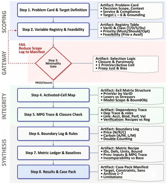
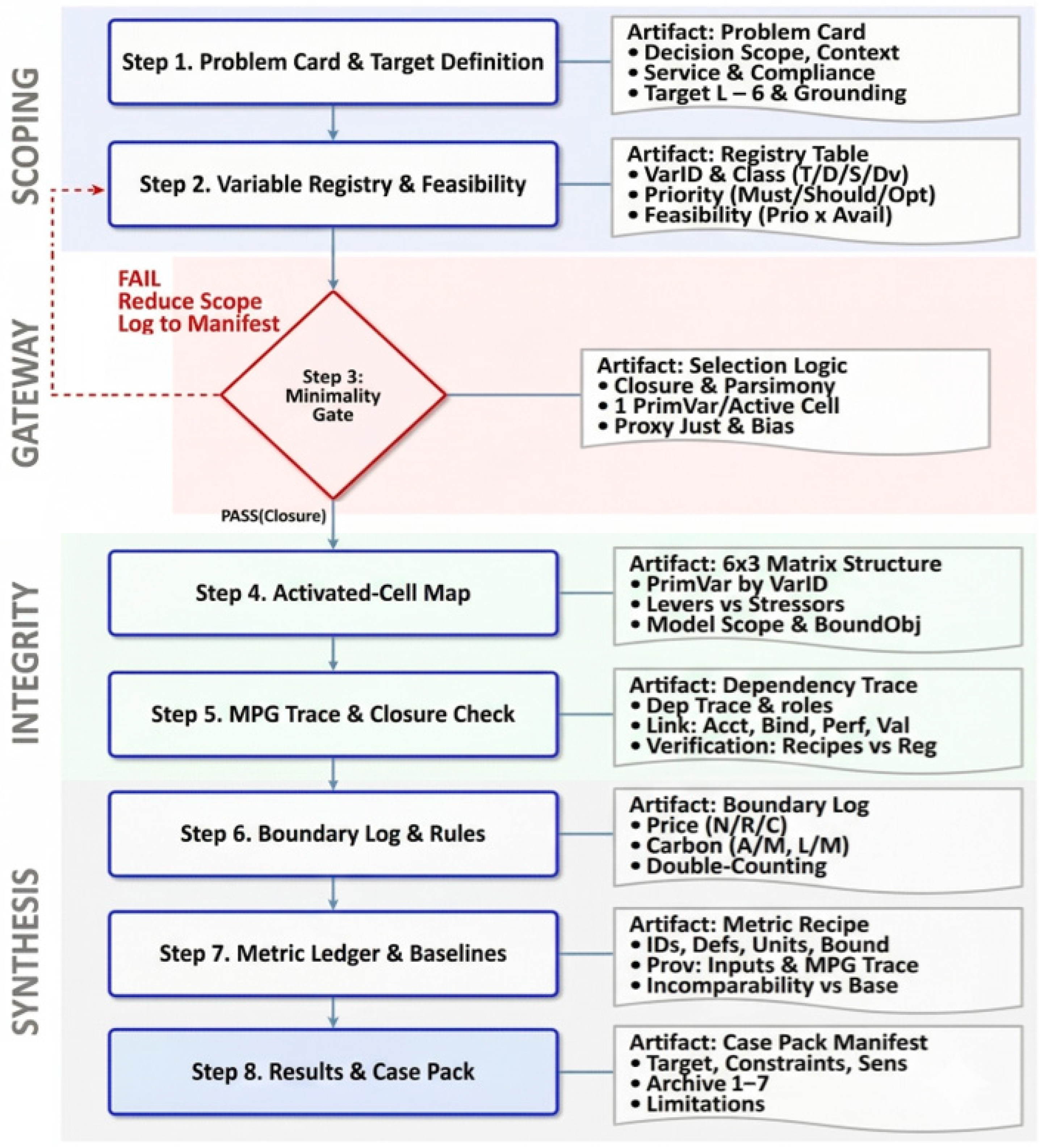
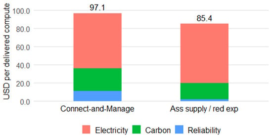
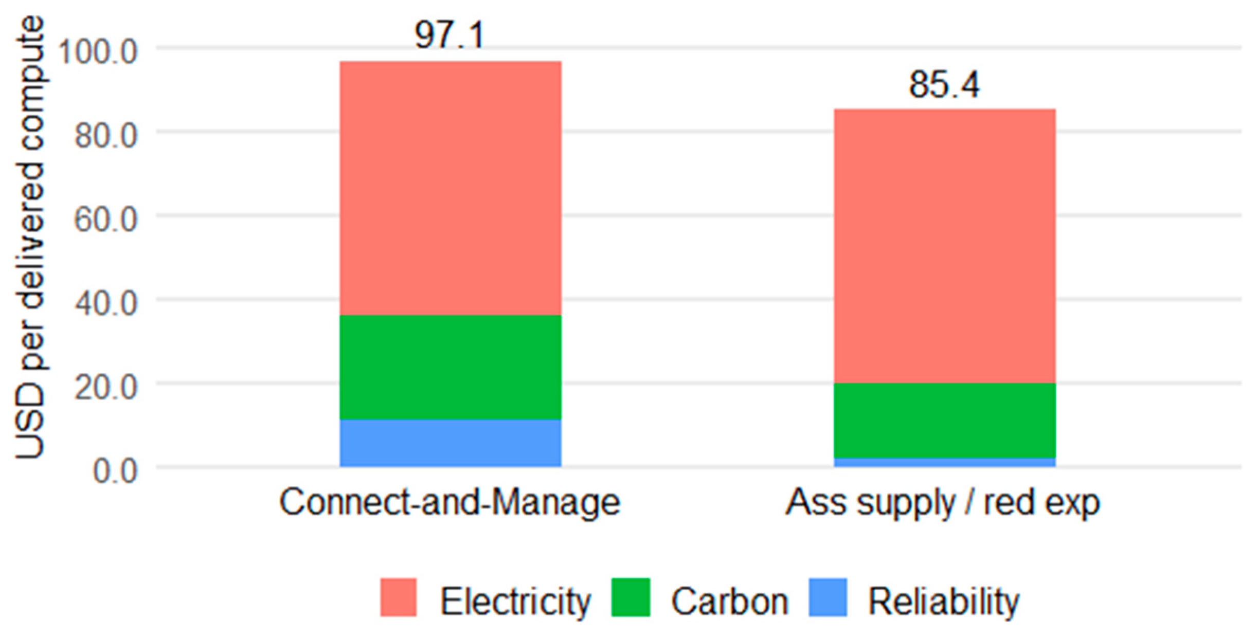
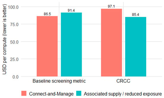
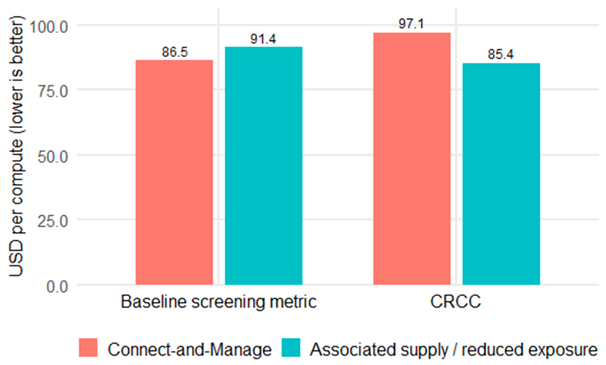
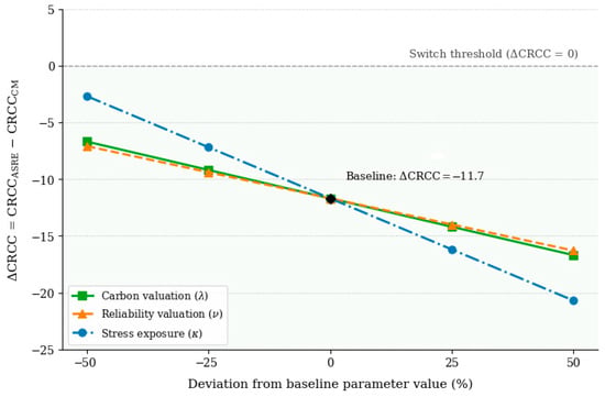
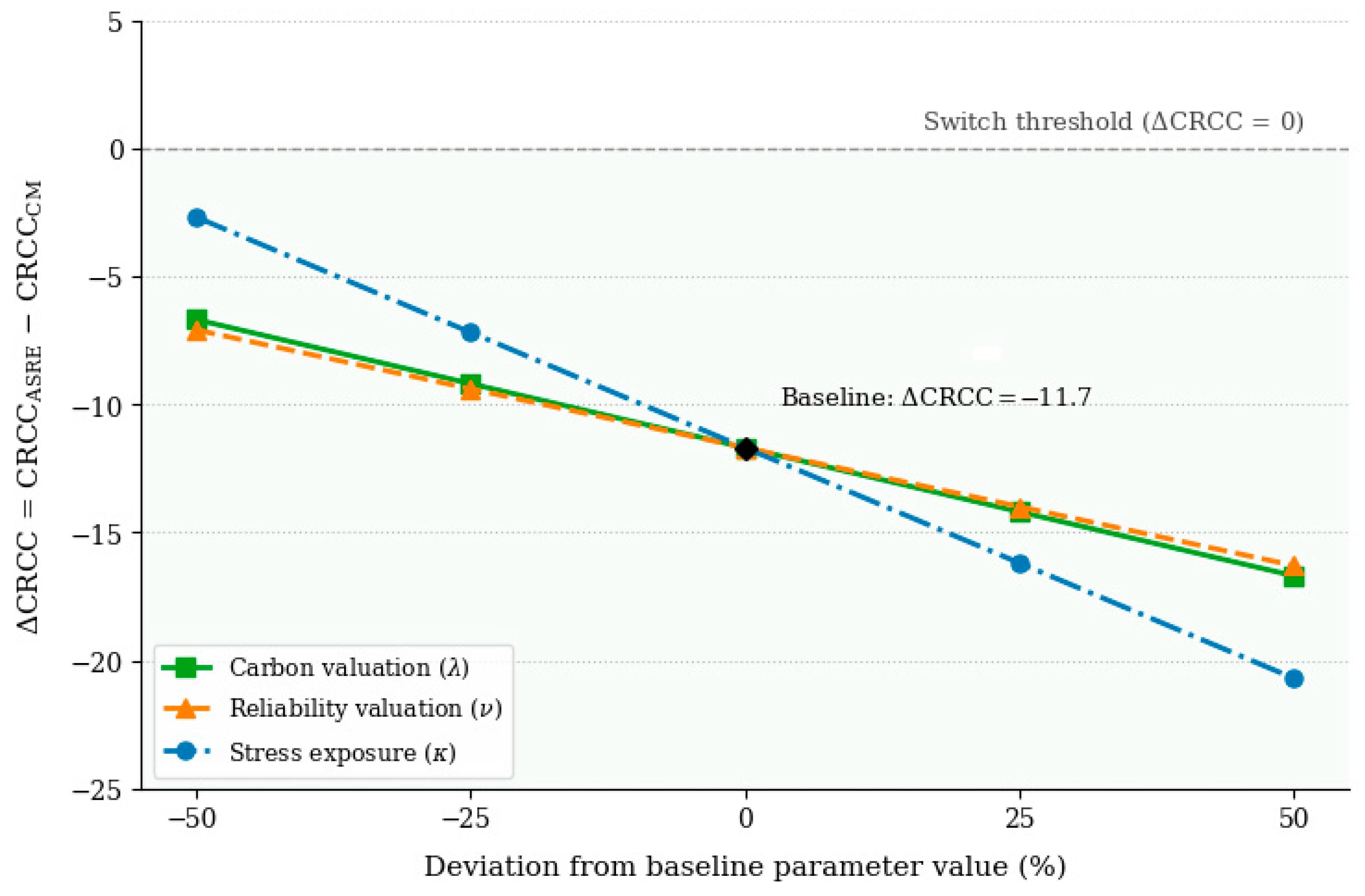
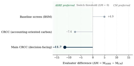
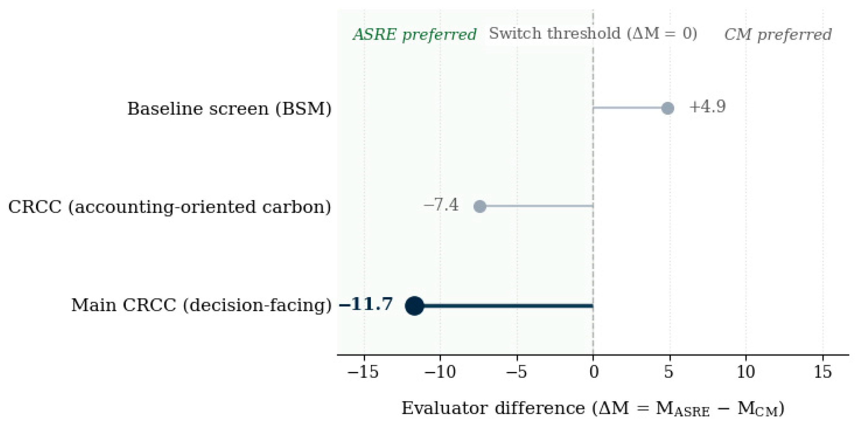

Disclaimer/Publisher’s Note: The statements, opinions and data contained in all publications are solely those of the individual author(s) and contributor(s) and not of MDPI and/or the editor(s). MDPI and/or the editor(s) disclaim responsibility for any injury to people or property resulting from any ideas, methods, instructions or products referred to in the content. |
© 2026 by the authors. Licensee MDPI, Basel, Switzerland. This article is an open access article distributed under the terms and conditions of the Creative Commons Attribution (CC BY) license.