Designing Predictive Models: A Comparative Evaluation of Machine Learning Algorithms for Predicting Body Carcass Fat in Ewes at Weaning

Abstract

Accurate estimation of Body Carcass Fat (BCF) is essential for evaluating the physiological condition of ewes. Traditional assessment via Body Condition Score (BCS) through palpation is inaccurate and subjective. BCF can now be predicted more precisely using objective measurements. This study presents a comparative analysis of eight machine learning (ML) models for predicting BCF in Coopworth ewes, using weight and RGB-image-based body measurements. Four non-linear regression methods and four neural network architectures were evaluated using a dataset of 74 ewes with 13 independent variables. The dataset was partitioned into training (52 ewes), validation (11 ewes), and testing (11 ewes) sets. The Gradient Boosting Regression achieved the highest predictive accuracy with an R² value of 0.9434 using body weight and width, followed by Ensemble Neural Network (R² = 0.9371) using body weight. The findings demonstrate the effectiveness of the Gradient Boosting Regression, Ensemble Neural Network and Random Forest tree-based approaches for morphometric prediction tasks in biological applications. BCF values obtained from image analysis were validated against those derived from computerized tomography (CT), considered the gold standard. These findings highlight the potential of image-guided, ML-driven models for objective, non-invasive, cost-effective assessment of ewe body composition in modern livestock systems.

1. Introduction

Body Carcass Fat (BCF) plays a vital role in animal health and nutrition in livestock management and on-farm biological research [1,2]. Effective monitoring of BCF throughout the reproductive cycle is part of the process of enhancing the state of the ewe and making informed decisions on-farm [3]. Traditional methods for BCF assessment often rely on subjective visual scoring such as Body Condition Scoring (BCS) or invasive procedures and costly methods such as Computed Tomography (CT) [4,5]. Although BCS is a simple method which is popular, it has been determined to be inappropriate in terms of measuring sheep condition, with its correlation to real fat content being wide ranging (R² between 0.01 and 0.72) [6,7,8,9,10,11,12,13,14]. This shows that more objective mechanisms are needed. Despite the fact that CT is the gold standard of BCF measurement, its expensive nature and logistical impacts make it unrealistic in routine on-farm practices [15].

Recent advances in machine learning have opened new possibilities for developing accurate predictive models using morphometric measurements [16,17,18,19,20,21,22,23,24,25,26,27]. However, most existing studies have focused on either traditional regression approaches or single machine learning techniques, lacking systematic comparisons between non-linear regression methods and neural network architectures using standardized datasets and validation protocols. The application of machine learning techniques to biological prediction problems has gained significant attention due to their ability to capture complex non-linear relationships between morphometric variables and physiological indicators [28,29]. The high correlation of BCS with BCF usually dominates ML models, obscuring the actual contribution of the image features. Thus, a strict comparative study that separates the predictive ability of the objective and image-derived features needs to be conducted [30].

Accurately assessing BCF at weaning is essential for evaluating reproductive performance [30,31,32,33]. Despite growing interest in mapping and forecasting BCF dynamics in ewes across production stages, and given its proven impact on flock performance, accurate assessment typically necessitates slaughter to obtain dissection metrics or reliance on CT imaging, both of which are logistically challenging and costly [15,26,34,35]. Although the prediction of BCF was investigated at pre-mating [26] and at pre-lambing [31], this study hypothesizes that a systematic comparison of the advanced machine learning models would help to find an efficient algorithm that can predict the BCF in ewes at weaning based on the combination of manual and image-derived morphometrical characteristics and be verified by a gold standard, that is, CT imaging. Thus, the purpose of the research is to conduct a thorough comparative analysis of eight different machine learning models in terms of non-linear regression and neural network designs to identify the most reliable and accurate model for predicting BCF. It will involve a strict feature validation analysis of both manual measurements and image features and a combination of the two to establish the research gaps in the present literature and contribute further to precision livestock management.

2. Materials and Methods

2.1. Data Collection

Morphometric and physiological data were systematically collected from a set of 74 Coopworth ewes (n = 74) aged 2–4 years at a critical time point during the production cycle: weaning (December). The ewes were shorn in late October and early November. To ensure the methodology could be applied across different fleece conditions, a standardized wool factor correction was implemented based on established fleece growth parameters for Coopworth ewes. Consequently, the staple length of wool was insignificant and its influence on body weight and image-based morphometric measurements was deemed to be negligible in this study. Reference data indicated that mature Coopworth ewes typically produce fleece weights of approximately 5.0 kg, with staple lengths ranging from 200 to 230 mm at shearing [36].

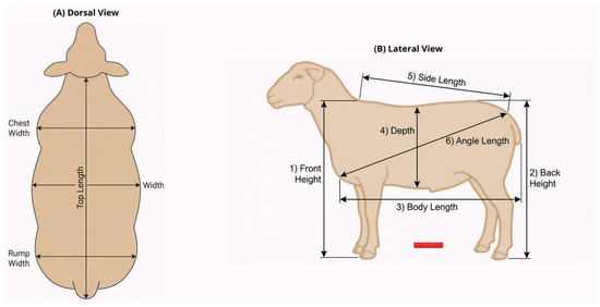
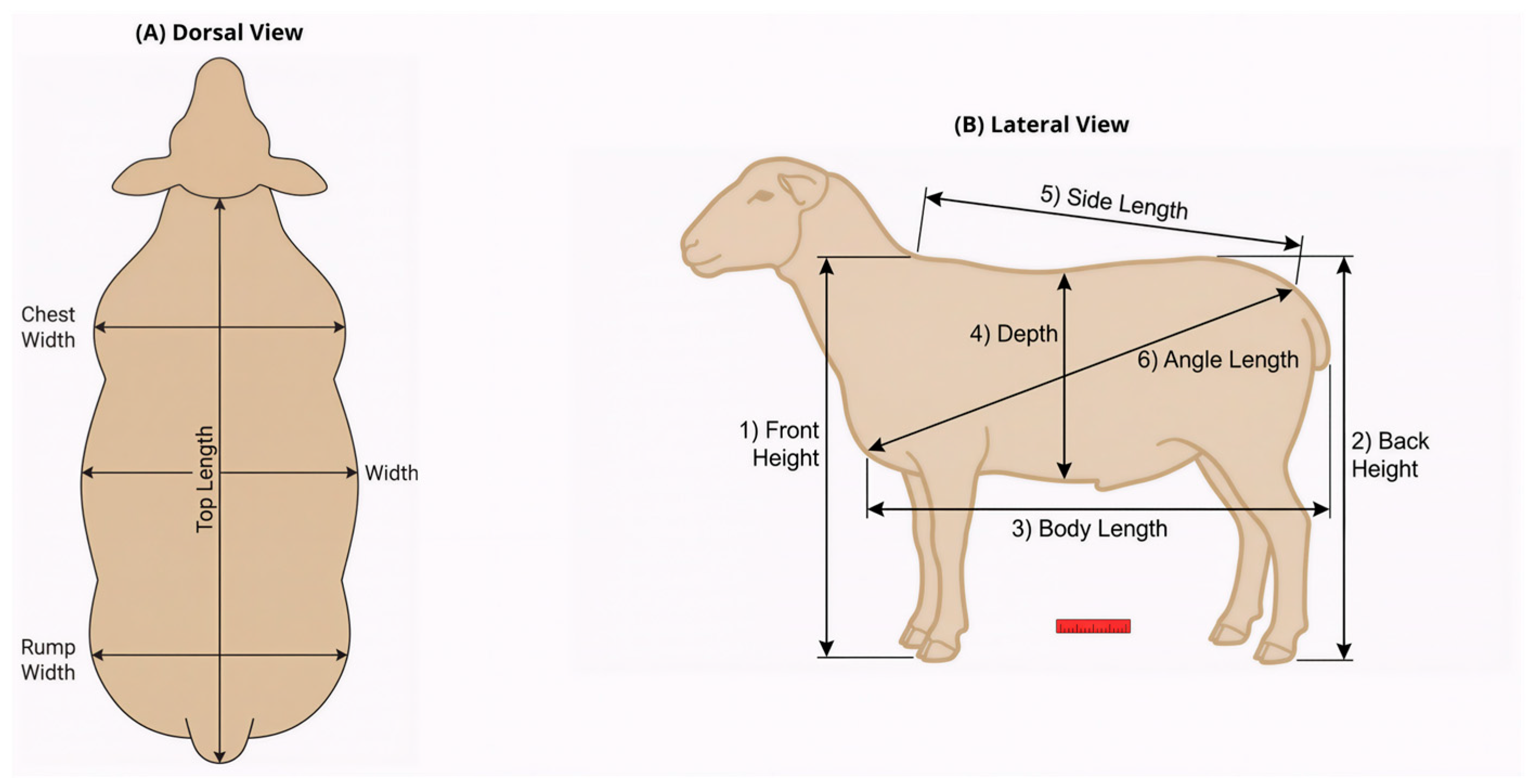
Measurement of Body Carcass Fat was done through CT imaging; a licensed CT operator was required to measure the fat through the use of standardized veterinary imaging protocols. CT scanning was used as the gold standard reference technique in the determination of BCF and it gave the exact volumetric measurement of adipose tissue distribution in the carcass. The quantification of BCF was determined with the help of the specialized imaging software (STAR 6.15, Lincoln University CT Lab, New Zealand), which offers extensive tools for tissue segmentation, volumetric analysis, and quantitative evaluation of the body composition parameters. Live weight was recorded using a calibrated electronic weighing system (Prattley Industries, New Zealand) with precision to ±0.1 kg. All weight measurements were conducted under standardized conditions to minimize environmental variability. Prior to morphometric assessment, ewes underwent a standardized 12 h fasting period, during which both feed and water access were restricted to minimize digestive tract fill variation and ensure consistent body conformation. Animals were individually positioned within a custom-designed metal restraint crate that maintained standardized posture while ensuring animal welfare and measurement repeatability. Body dimension measurements of Depth, Body Length, Height, Angle Length, and Top Length were obtained using a precision-engineered measuring ruler featuring millimeter-scale graduations. The ruler incorporated a fixed reference point and an adjustable sliding component to ensure accurate and consistent linear measurements across various body measurements. An image processing application was built to extract morphometric parameters from the captured images, as shown in Figure 1. Dorsal view parameters included top body length (cranial–caudal dimension), front width (maximum thoracic width), body width (maximum abdominal width), rump width (maximum pelvic width) and top area (cm²). Lateral view parameters included front height (withers height measurement), back height (rump height measurement), body depth (dorsal–ventral dimension at maximum depth), body length (from twist to breast), side length (diagonal measurement from forearm to rump), angle length (from hock to neck) and side area (cm²). The image processing algorithm incorporated automatic scaling based on reference markers within each image, ensuring dimensional accuracy and eliminating perspective distortion effects.

Figure 1. Localization of morphometric measurement on the dorsal (top) and lateral (side) views.

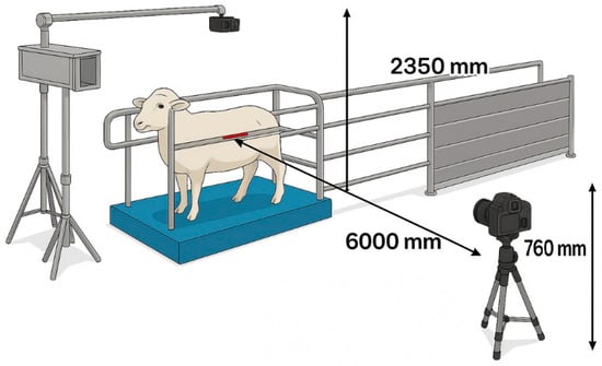
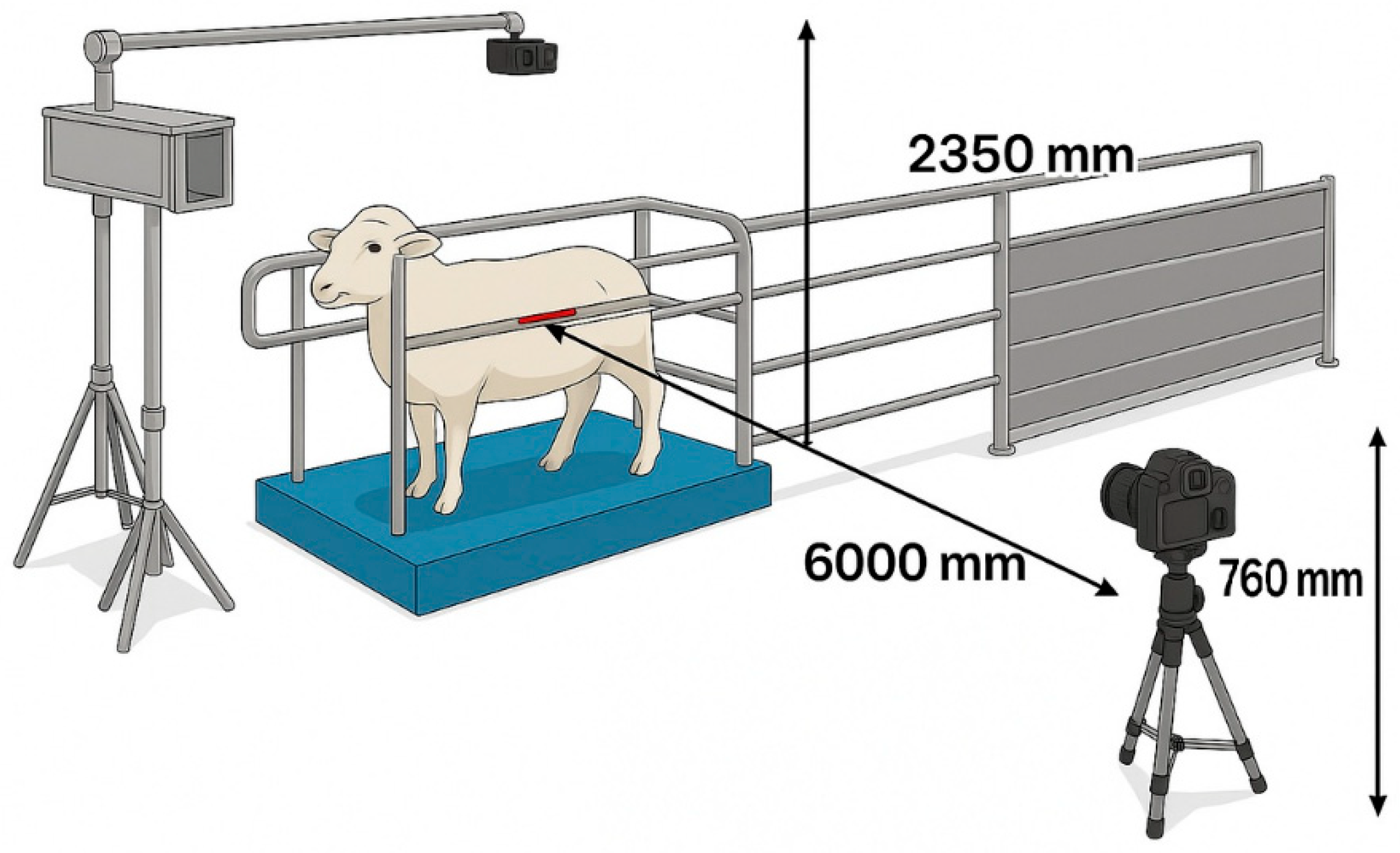
All measurements were recorded in millimeters with precision to ±0.1 mm, and each parameter was measured in triplicate to assess measurement repeatability and reduce operator error. A dual-camera imaging system was employed to capture comprehensive morphometric data from orthogonal anatomical perspectives. The dorsal imaging apparatus consisted of a GoPro Hero 7 action camera (GoPro Inc., San Mateo, CA, USA) equipped with a 12-megapixel CMOS sensor, positioned at a vertical height of 2350 mm above the ground plane to ensure complete dorsal body coverage within the field of view. For lateral morphometric analysis, a Canon EOS 750D digital single-lens reflex camera (Canon Inc., Tokyo, Japan) featuring a 24.2-megapixel APS-C CMOS sensor was utilized. The lateral imaging system was positioned at a horizontal distance of 6000 mm from the subject’s sagittal plane and mounted at a height of 760 mm above ground level to optimize anatomical landmark visibility and minimize perspective distortion. Both cameras were calibrated and synchronized to ensure temporal consistency during image acquisition, with standardized exposure settings maintained throughout the data collection period to ensure uniform image quality and morphometric measurement accuracy, as shown in Figure 2.

Figure 2. Experimental setup for RGB image-based morphometric assessment of sheep body carcass fat analysis.

2.2. Image Processing Application

An image processing application was implemented using the OpenCV computer vision library to extract morphometric features from the acquired RGB images. The processing workflow had multiple sequential operations including image acquisition, color space transformation, thresholding, morphological processing, geometric correction, segmentation, and filtering algorithms to ensure robust feature extraction and measurement accuracy.

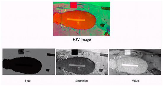
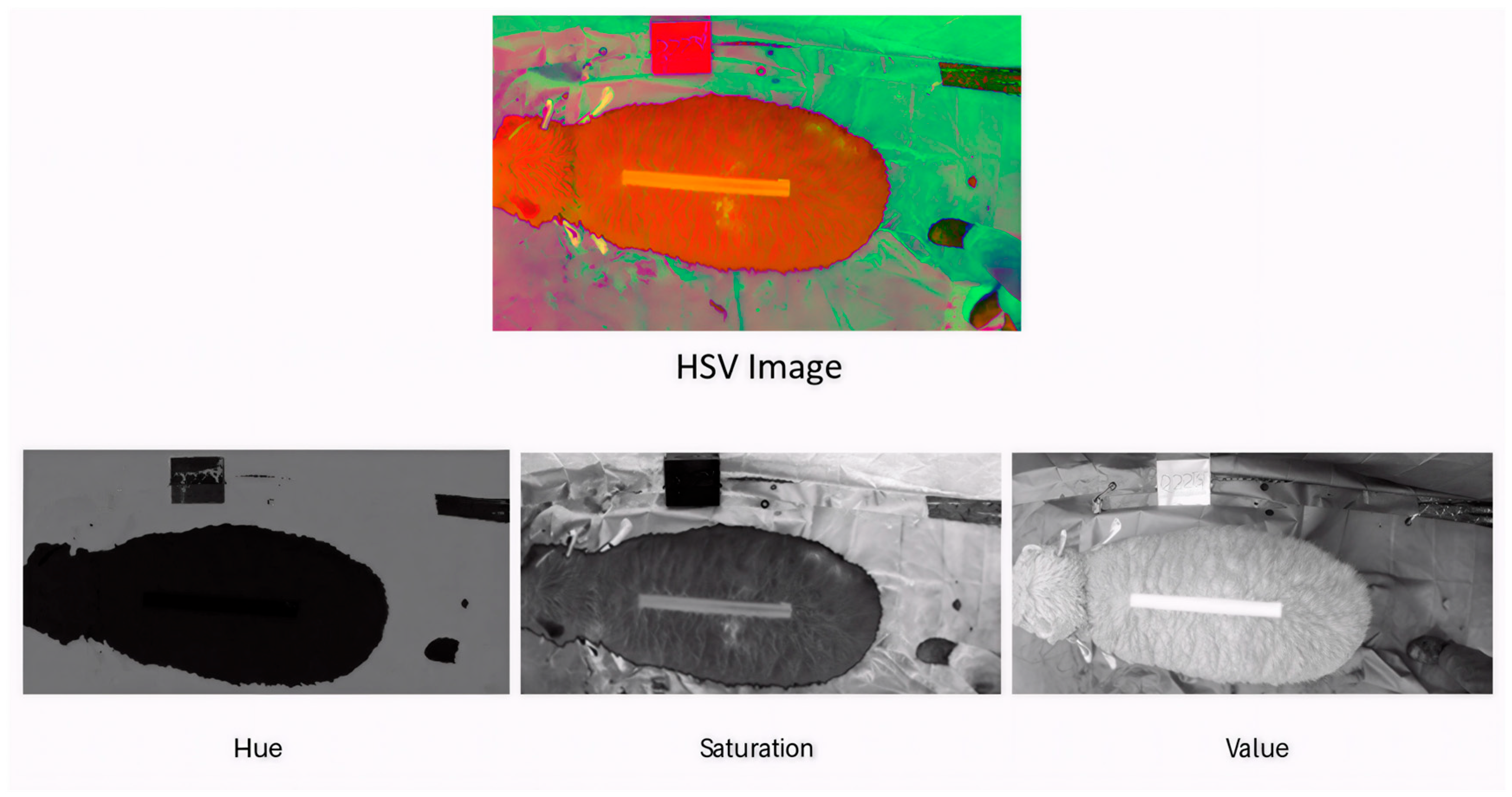
The fundamental preprocessing step involved converting the source RGB images to the HSV (Hue, Saturation, Value) color space to enhance segmentation performance and reduce sensitivity to illumination variations. This transformation was selected based on the superior performance of HSV color space in biological image analysis applications, where lighting conditions may vary and color consistency is critical for accurate morphometric measurements, as shown in Figure 3. HSV color space decomposition separates chromatic information from luminance data, providing three distinct channels that represent different aspects of color perception. The hue component encodes the dominant wavelength of the color, corresponding to the perceived color type, and is represented as an angular measurement on the color wheel ranging from 0° to 360°. Within this angular representation, specific color ranges are defined: red occupies 0–60°, yellow spans 61–120°, green encompasses 121–180°, cyan covers 181–240°, blue extends from 241 to 300°, and magenta completes the spectrum from 301 to 360°. The saturation channel quantifies the purity or intensity of the color, representing the degree to which the hue is diluted by white light. Saturation values range from 0 to 100%, where higher values indicate more vivid and intense colors, while lower values approach achromatic gray. This channel proves particularly valuable for biological image segmentation as it effectively distinguishes between the subject and background elements regardless of lighting variations. The value component represents the brightness or luminance intensity of the color, functioning as a measure of the overall lightness independent of the chromatic content. Value measurements span from 0 (complete darkness) to 100 (maximum brightness), providing essential information for contrast enhancement and edge detection algorithms.

Figure 3. Converting the top image to Hue, Saturation, Value (HSV) color space.

Following the HSV color space transformation and saturation channel extraction, binary thresholding was implemented as the critical segmentation step to convert the processed grayscale image into a binary representation suitable for morphometric feature extraction. This binarization process serves as the foundation for subsequent shape analysis and measurement algorithms by establishing clear boundaries between the subject (sheep) and background regions.

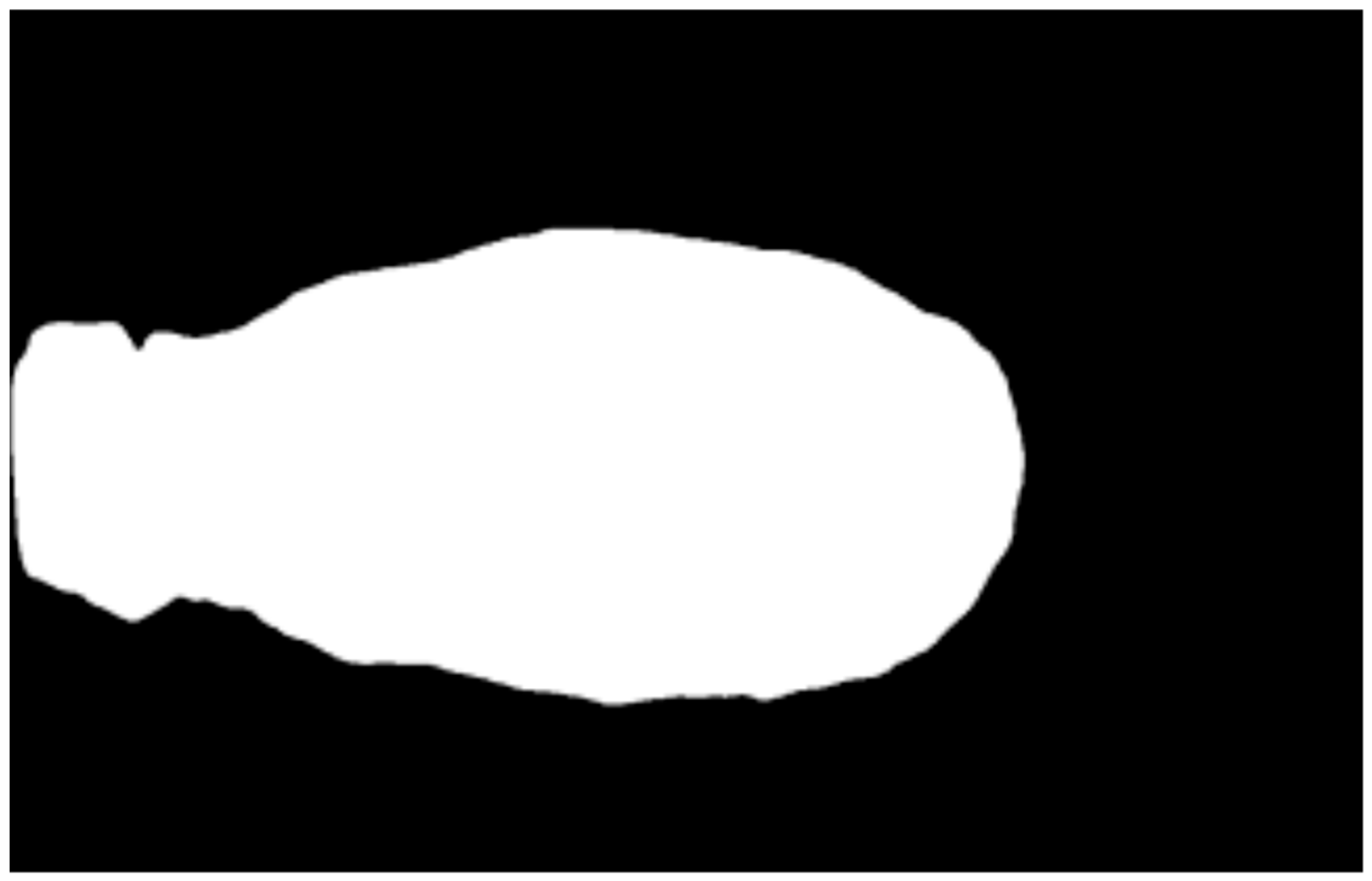
Then, the image was converted to black and white by applying the threshold function that converts any pixel with a value greater (lighter) than the selected value into white and the lower values (dark) into black, as shown in Figure 4. The threshold value was empirically determined and set to 150 on the standard 8-bit grayscale intensity scale (0–255 range) following systematic evaluation of segmentation performance across representative sample images. This value was chosen after testing all images due to similar illumination conditions during image capturing, and was observed to produce clear segmentation when converting from grayscale images into binary images.

Figure 4. Converting the top image into black-and-white color space.

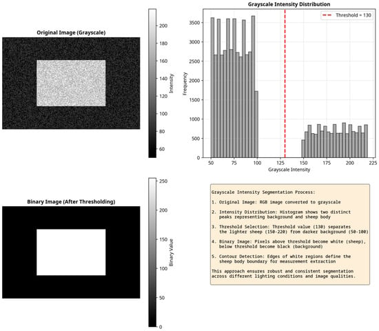
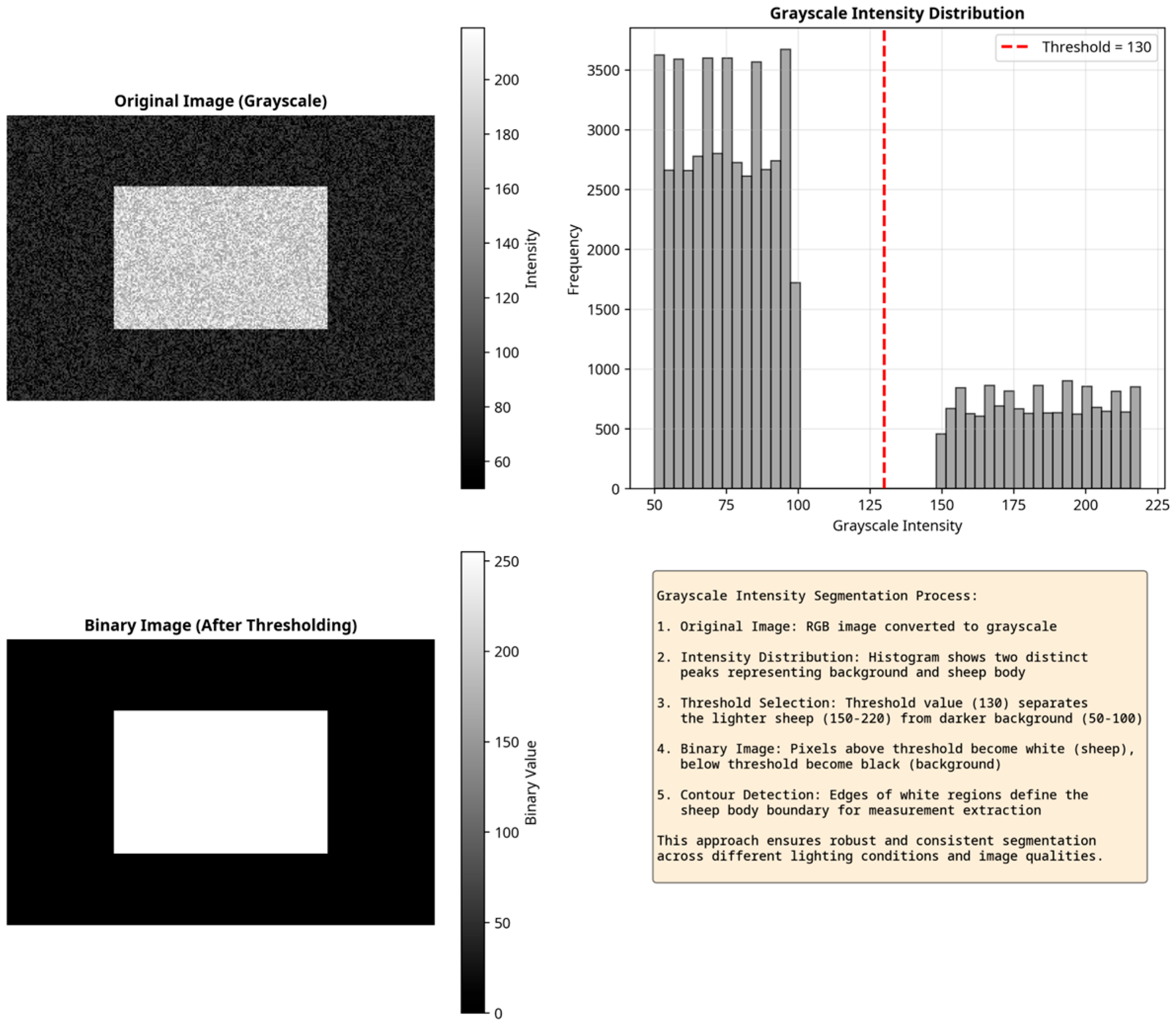
In order to explain the segmentation procedure, Figure 5 shows the application of grayscale intensity in isolating the sheep body. The histogram indicates that it is a bimodal distribution, where the less intense mode is the background and the intense one is the lighter group of sheep. We can also filter out the contours of the sheep by choosing a threshold between these two peaks, creating a binary mask which is used to isolate the sheep and the background, and using it to accurately isolate the contours of the sheep.

Figure 5. The segmentation process based on the intensity of the grayscale. Original grayscale image. Histogram of grayscale intensities with the distribution of two modes and the chosen threshold. Output of thresholding binary image.

Following binary thresholding, a series of morphological operations were systematically applied to both dorsal- and lateral-view images to enhance segmentation quality and eliminate noise artifacts. The fundamental morphological operations of erosion and dilation were implemented as complementary processes to achieve optimal noise reduction and boundary preservation. Erosion operations systematically removed pixels from object boundaries by applying a structuring element that evaluates local pixel neighborhoods, effectively shrinking object regions and eliminating small noise artifacts that do not conform to the expected morphological characteristics of the target subject. Then, dilation operations were applied to restore the original object dimensions and compensate for the boundary shrinkage introduced during the erosion phase [37]. The number of pixels added or removed from the objects depended on the size and shape of the structuring element used to process the image.

To extract the morphometric features of the RGB images obtained, an image processing program was developed based on the OpenCV (Open Source Computer Vision Library) libraries to find all objects in the image, isolate the largest object and make it the target object. This method was implemented using a for-loop statement that checks all contours (objects) and returns an image containing the largest object as a points list (vector). The application used code from OpenCV’s built-in method ‘findContours’ that returns a list of contours (objects) in the image. The variable maxSize was then used to find the maximum size of the contours and the variable maxSizeIndex was used to point to the largest contour. The for-loop checks every contour in the contours list and compares its size with the variable maxSize; if the new contour size is bigger, its size is defined as the maximum size and its index as the maxSizeIndex. At the end of the loop, the variable maxSizeIndex will have the index of the contour that has the maximum size; it then draws only on a new black image with one object, representing the largest object, and returns the object as a point list. After converting the top images from greyscale to binary images and once the binary object of the ewe (foreground = 1, background = 0) had been obtained, neck and head were automatically removed, depending on the local body width (widest distance around the mass center) when compared to the maximum width of the ewe. The neck and head were removed by cutting lines smaller than 70% of the body width, and then the largest object was obtained, to isolate the ewe’s body from the background.

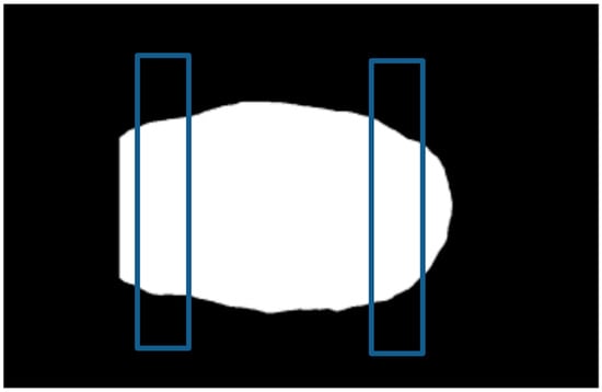
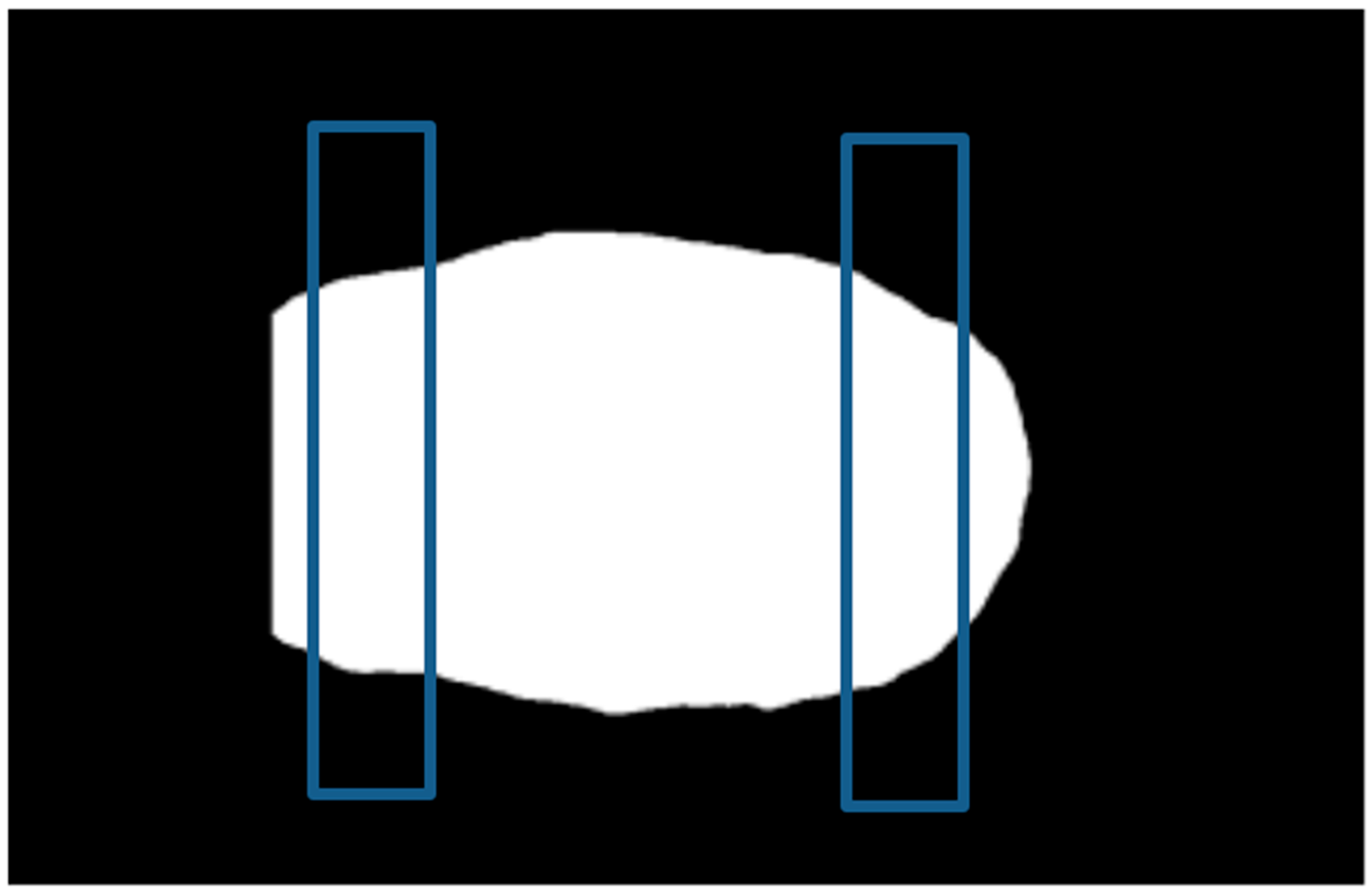
After the extraction of the sheep’s body, a smooth filter was applied to the images to smooth the sheep’s outlines from the noisy border of the segmentation process. Once the large object was extracted and all noise had been fixed, the image was ready to start being measured, as shown in Figure 6.

Figure 6. Chest width and rump width calculation—top image.

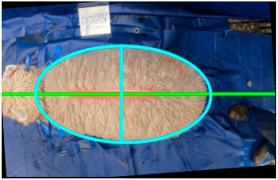
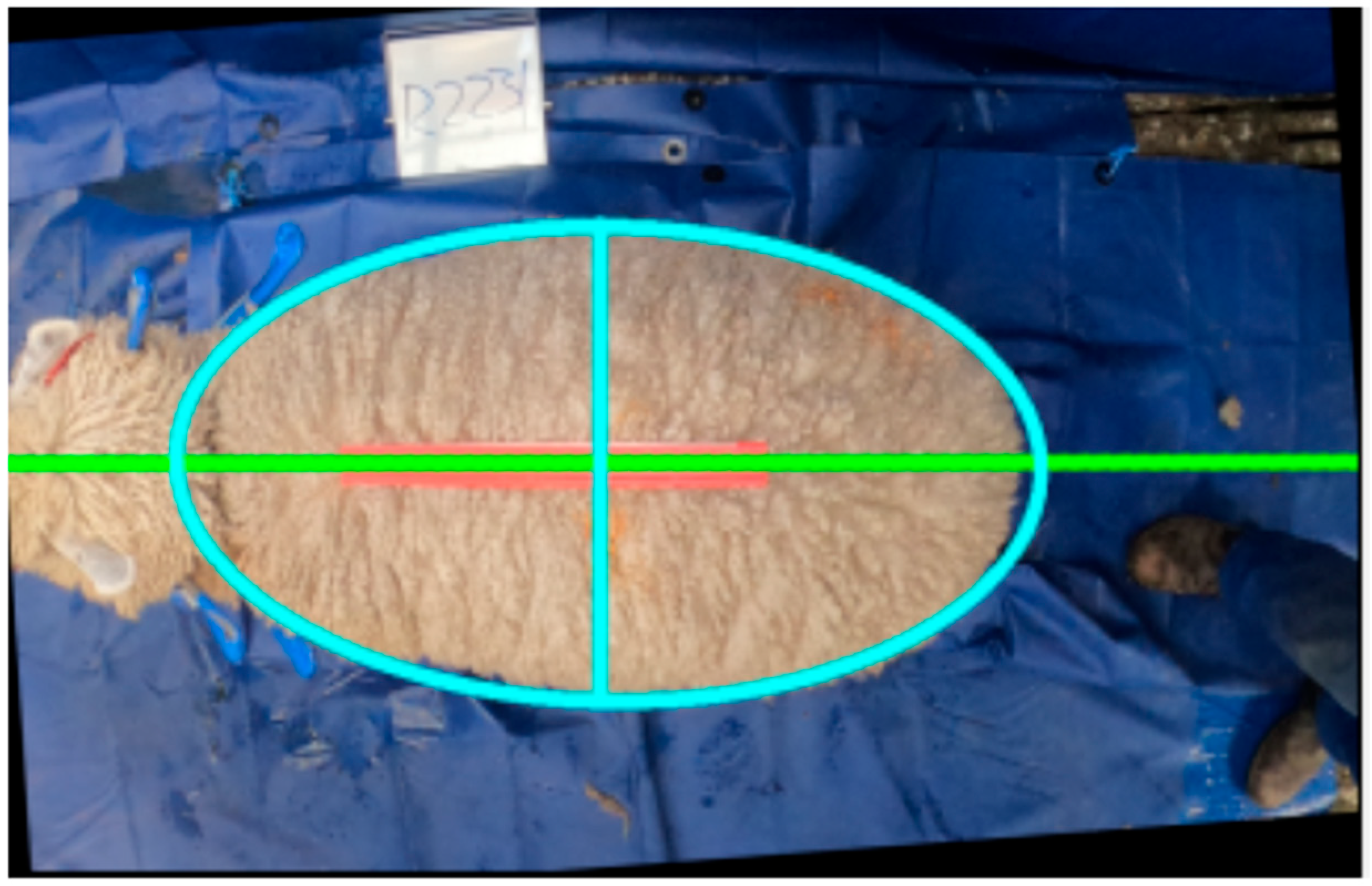
The geometric centroid of the segmented sheep body contour was computed through mathematical moment analysis, utilizing the fundamental principles of spatial moment calculations to determine the center of mass coordinates, as shown in Figure 5. Spatial moment calculation is a systematic way of measuring the distribution of pixel intensities of pixels within the region of the segmented object, and the result is computed by weighted sums of coordinates which reflect the geometric features of the sheep body contour; thus, the centroid is determined and morphometric measures are calculated. All morphometric measurements were initially computed in pixel units within the digital image coordinate system, necessitating systematic conversion to physical measurement units for meaningful biological interpretation and analysis. The dimensional calibration process implemented a standardized pixel-to-centimeter conversion protocol to transform digital measurements into physically meaningful morphometric parameters.

All measurements were calculated in pixels, then converted to cm. A red ruler was used as a scale in pixels and as a reference value since it has a known length in cm (40 cm). All measurement values were divided by the reference length in pixels and multiplied by 40 to get the values in cm. The last step was to display all values in cm for the top and side images, as shown in Figure 7.

Figure 7. Determining the center of mass and calculating the top length and top area—top image.

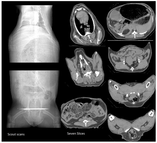
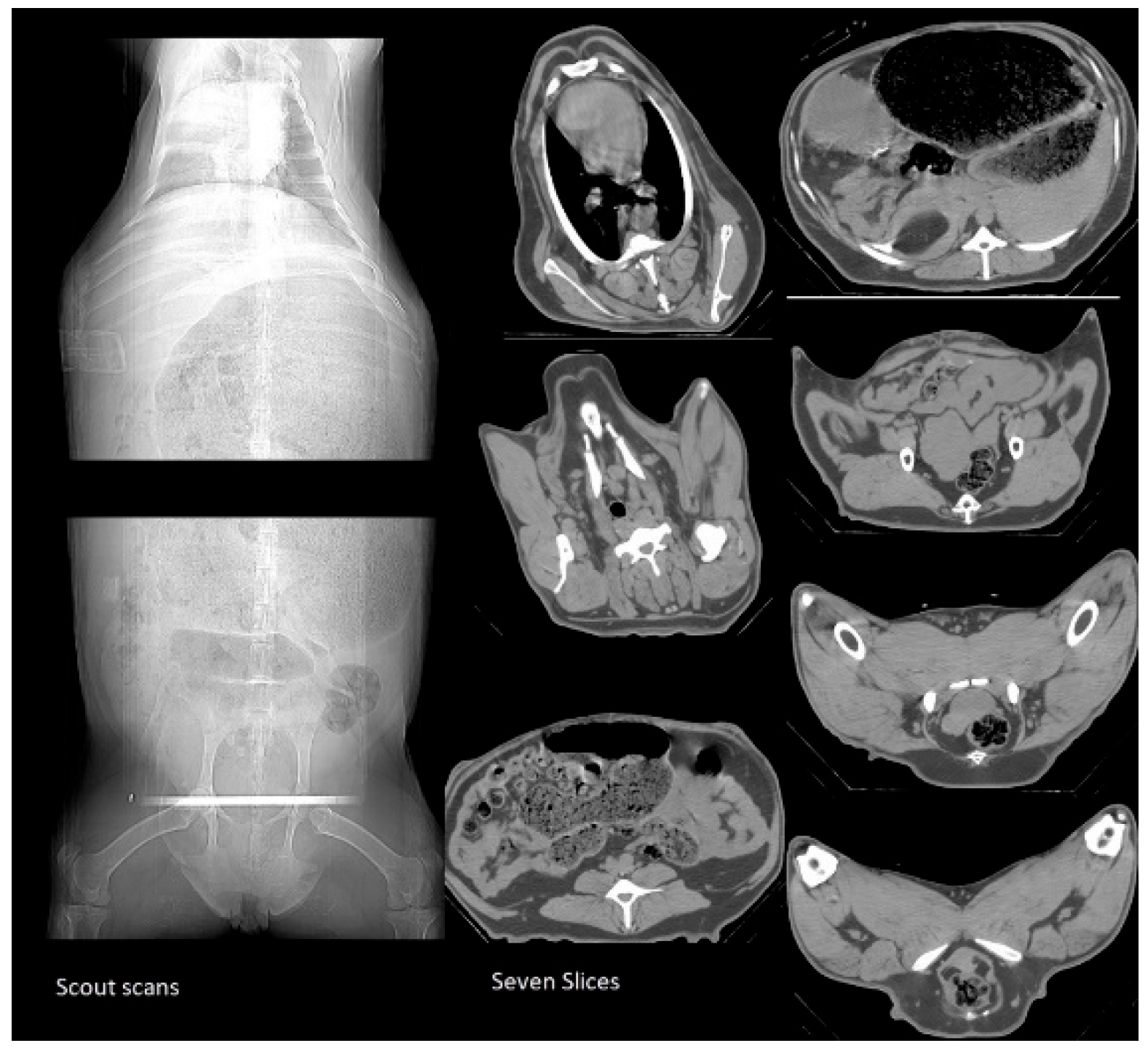
CT imaging was conducted following the established Lincoln University Standard Operating Procedure 83 (SOP 83) for livestock CT scanning, as previously validated and described by [2]. This standardized protocol ensures consistent imaging parameters, animal welfare compliance, and reproducible data acquisition across all experimental subjects. BCF quantification was performed using a GE ProSpeed CT console model CT750 HD class and STAR 6.15 specialized imaging software [38], which provides comprehensive tools for tissue segmentation, volumetric analysis, and quantitative assessment of body composition parameters. The software enables precise differentiation between adipose tissue, lean muscle mass, and bone structures through advanced density-based segmentation algorithms. All CT imaging procedures were conducted by a licensed radiological technologist holding current certification from the National Radiation Laboratory for the operation of ionizing radiation equipment. The scout scan determines the seven sites with positions marked for the seven cross-sectional tomograms: ischium, femur, hip, fifth and second lumbar vertebrae (LV5 and LV2) and eighth and sixth thoracic vertebrae (TV8 and TV6). BCF areas are shown as dark grey, lean as light grey, bone as white and air as black, as shown in Figure 8.

Figure 8. Ewe CT scout scans and the seven slices.

2.3. Data Partitioning

The dataset was partitioned using stratified sampling to maintain representative distributions across all subsets: training set: 52 samples (70.3%), validation set: 11 samples (14.9%), and testing set: 11 samples (14.9%). This partitioning strategy follows best practices for machine learning model evaluation [39] and ensures robust performance assessment.

2.4. Non-Linear Regression and ANN Techniques

Four advanced non-linear regression techniques, Polynomial Regression (Poly), Support Vector Regression (SVR), Random Forest Regression (RF) and Gradient Boosting Regression (GBR), were evaluated to predict BCF from body measurements. The Poly technique used an extension of linear regression that includes polynomial terms to model non-linear relationships between the predictors and the response. A second-order polynomial was used to strike a balance between model complexity and interpretability [40]. The SVR used kernel functions to map the input features to a higher dimension to perform non-linear pattern recognition [41]. The SVR was selected for its effectiveness in handling non-linear relationships. The RF algorithm was used as it works by combining multiple decision trees using bootstrap aggregating to minimize overfitting and increase test-time performance [42]. The algorithm generated several decision trees and merged their predictions together. Then, GBR was investigated to build models sequentially, where each model compensated for the mistakes of the previous model [43]. The algorithm minimizes a loss function through gradient descent.

In addition to the four non-linear regression models, four neural network techniques (Multi-Layer Perceptron, Deep Neural Network with Dropout, Regularized Neural Network, and Ensemble Neural Network) were evaluated [44]. The Multi-Layer Perceptron (MLP) architecture consisted of three hidden layers with decreasing neuron counts to create a funnel structure for feature extraction [45]. The deep neural network with dropout used a deeper architecture that was incorporated with a dropout regularization technique to prevent overfitting [46]. The Regularized Neural Network (RNN) technique is based on reducing overfitting and was used to modify the learning model, with better outcomes and higher performance [47]. Then, the Ensemble Neural Network (ENN) technique was used to combine multiple neural networks with slightly different architectures to improve prediction robustness and performance [48]. The performance and accuracy of the models were assessed using Coefficient of Determination (R²), Mean Squared Error (MSE), Root Mean Squared Error (RMSE) and Mean Absolute Error (MAE) [49]. Statistical significance was determined by testing the accuracy of the models and comparing the performances between the models. Then, a 10-fold cross-validity method was adopted to ensure stable estimation of BCF and prevent overfitting bias in model selection. The data was randomly divided into 10 subsamples of equal size. Among the 10 subsamples, one subsample was selected as the testing data to validate the model, with the rest of the 9 subsamples serving as the training data. This cross-validation procedure was repeated 10 times, whereby the 10 subsamples were utilized once as the validation data. The 10 points showing the folds were averaged to obtain one estimation. Moreover, bootstrapping with 1000 iterations was used to obtain a 95% confidence interval of the R² values in order to measure the uncertainty of the performance estimates.

3. Result

3.1. Descriptive Statistics

The dataset exhibited considerable variability in morphometric measurements, reflecting the diversity of the sample population. BCF values ranged from 0.885 to 17.649, with a mean of 5.105 ± 3.454, as shown in Table 1.

Table 1. Descriptive statistics of dataset variables.

Variable	Mean	Std Dev	Min	Max	Skewness	Kurtosis
BCF—kg	5.105	3.454	0.885	17.649	1.847	3.421
Weight—kg	59.735	8.993	44.000	88.500	0.892	0.654
Angle Length—cm	75.324	4.892	63.000	84.200	−0.123	−0.456
Side Length—cm	69.845	5.234	60.800	82.600	0.234	−0.123
Body Length—cm	74.567	4.123	68.000	82.100	0.345	−0.234
Height—cm	62.345	3.456	55.800	69.700	0.123	−0.345
Back Height—cm	63.234	4.567	55.700	71.700	0.234	−0.123
Depth—cm	37.123	3.234	32.600	43.300	0.345	−0.234
Side Area—cm2	2456.78	234.56	2137.60	2924.30	0.123	−0.345
Top Length—cm	75.234	4.567	67.500	85.200	0.234	−0.123
Width—cm	31.234	2.345	28.800	37.200	0.345	−0.234
Rump Width—cm	29.455	2.404	20.000	34.300	−0.123	0.456
Front Width—cm	26.091	2.628	22.300	33.600	0.234	−0.123
Top Area—cm2	1793.13	183.68	1354.30	2369.90	0.345	−0.234

3.2. Application Uncertainty Tests

The first test was conducted to determine the accuracy of the image-derived measurements, as shown in Table 2. The following measurements were manually obtained with a ruler: Depth, Body Length, Height, Angle Length, Top Length and Width. They were compared with the same measurements obtained from the images. The result showed an average acceptable difference of 3.6% [50].

Table 2. Average absolute error between ruler and image measurements.

Measurements	Depth	Body Length	Height	Angle Length	Top Length	Width
Error %	2.5%	3.6%	3.5%	3.7%	4.5%	3.5%
Average Error%	3.6

The second test aimed to test the uncertainty of the image processing measurements of two images for the same ewe. A set of 12 ewes with differences in live weight, BCS and body size was chosen, and three lateral and dorsal measurements were taken for each ewe. Two images were selected for each ewe, where the ewe was in a good position (not turning to the right or left). An average mean difference of 1% for the application measurements of two images for the same animal among the 12 ewes is shown in Table 3 and Table 4. The results show a variance of less than +/−21 mm for all body measurements, with more than 95% of the results having a variance of +/−10 mm. The maximum variance was +20.7 mm for the top length.

Table 3. Variance test of multiple images for each ewe (mm)—lateral view.

Depth			Side Length			Height			Angle Length
1st Image	2nd Image	Δ	1st Image	2nd Image	Δ	1st Image	2nd Image	Δ	1st Image	2nd Image	Δ
371.92	376.24	−4.32	696.98	700.12	−3.14	632.11	634.76	−2.65	748.09	755.45	−7.36
339.43	322.79	16.64	696.03	697.76	−1.73	653.64	653.11	0.53	806.56	795.27	11.29
377.1	365.89	11.21	652.85	660.11	−7.26	643.73	640.95	2.78	746.23	758.35	−12.12
362.96	382.04	−19.08	716.13	712.69	3.44	662.01	656.24	5.77	722.87	736.51	−13.64
350.77	362.08	−11.31	718.04	710.93	7.11	642.13	642.44	−0.31	813.62	820.48	−6.86
345.49	356.75	−11.26	717.79	720.07	−2.28	624.31	624.86	−0.55	805.01	793.11	11.9
364.39	369.03	−4.64	702.99	701.01	1.98	648.15	656.21	−8.06	802.47	791.35	11.12
377.01	372.88	4.13	699.06	699.06	0	603.82	601.26	2.56	687.31	686.08	1.23
334.99	345.07	−10.08	749.22	742.88	6.34	626.66	619.62	7.04	715.79	727.37	−11.58
367.82	371.12	−3.3	706.09	699.77	6.32	600.07	598.44	1.63	806.98	799.75	7.23
399.01	401	−1.99	709.91	704.23	5.68	572.48	574.96	−2.48	811.32	793.28	18.04
361.03	361.03	0	635.03	627.71	7.32	648.69	656.06	−7.37	696.61	681.99	14.62
Max, min Δ		+16.64, −19.08	+7.32, −7.26			+7.04, −8.06			+18.04, −13.64
Mean diff.		2%	1%			1%			1%

Table 4. Variance test of multiple images for each ewe (mm)—dorsal view.

Top Length			Rump Width			Front Width			Width
1st Image	2nd Image	Δ	1st Image	2nd Image	Δ	1st Image	2nd Image	Δ	1st Image	2nd Image	Δ
770.08	770.08	0	300.92	300.81	0.11	290.83	300.05	−9.22	310.58	310.47	0.11
790.25	800.88	−10.63	300.70	310.68	−9.98	290.94	300.37	−9.43	320.78	330.10	−9.32
820.62	820.62	0	320.98	330.20	−9.22	300.16	300.16	0	330.43	330.32	0.11
840.90	850.01	−9.11	310.68	310.68	0	290.07	290.18	−0.11	320.23	320.23	0
850.34	850.34	0	320.76	320.87	−0.11	290.07	280.85	9.22	330	320.67	9.33
790.58	800.23	−9.65	280.09	280.53	−0.44	250.59	250.81	−0.22	290.19	290.41	−0.22
850.01	850.88	−0.87	320.22	320.66	−0.44	280.63	280.42	0.21	320.02	320.13	−0.11
790.68	780.82	9.86	330.42	330.42	0	270.87	280.20	−9.33	310.58	310.69	−0.11
880.92	860.32	20.6	330.96	350.37	−19.41	320.00	320.44	−0.44	350.71	360.15	−9.44
870.29	870.62	−0.33	350.92	360.03	−9.11	320.11	320.22	−0.11	350.28	350.39	−0.11
830.27	830.27	0	340.29	340.50	−0.21	320.98	330.31	−9.33	350.82	350.93	−0.11
830.16	830.49	−0.33	320.33	320.33	0	270.98	280.20	−9.22	310.58	310.69	−0.11
Max, min Δ		+20, −10.63	+0.11, −19.98			+9.22, −9.43			+9.33, −9.44
Mean diff.		1%	1%			2%			1%

3.3. Technical Specifications

The technical specifications of the eight machine learning models used in the comparative analysis, such as hyperparameters, kernels for non-linear models and nodes, activation functions, regularization and epochs, are represented in the following Table 5 and Table 6. Hold-out validation was used to ensure robust and iterative tuning, and was then applied to select the last set of hyperparameters, where the models with the best balance between training R² and validation R² were given a higher priority. The hyperparameters in each model, as shown in Table 5, were identified using a systematic grid search with 10-fold cross-validation to identify the best hyperparameters in our dataset. In the case of SVR, grid search was used to find the best regularization (C=100), kernel coefficient (gamma = 0.1) and tolerance (epsilon = 0.1) of the RBF kernel. In the case of GBR and RF ensemble models, 100 trees were identified as the best number of trees. The best learning rate was 0.1 and the best max depth was 3 to ensure that GBR performance did not overfit, whereas RF could best use the default settings of max depth (max depth = None), which is common with this algorithm. In the case of Polynomial Regression, a degree of 2 was selected, because higher orders of degree would lead to the instability of higher-order polynomials [51].

Table 5. Technical specifications—non-linear regression models.

Model	Hyperparameters	Kernel
SVR	C = 100, gamma = 0.1, epsilon = 0.1	Radial Basis Function (RBF) Kernel
GBR	n_estimators = 100, learning_rate = 0.1, max_depth = 3	Ensemble of 100 Decision Trees
RF	n_estimators = 100, max_depth = None	Ensemble of 100 Decision Trees
Poly	Degree = 2	Linear Regression on 2nd-degree polynomial features

Support Vector Regression (SVR), Gradient Boosting Regression (GBR), Random Forest Regression (RF), Polynomial Regression (Poly).

Table 6. Technical specifications—neural network models.

Model	Nodes	Activation	Regularization	Dropout Ratio	Epochs (100 Max)
MLP	Input -> (64) -> (32) -> Output (1)	ReLU	None	0.0	57—manual features. 36—image features 20—combined
DNN	Input -> (128) -> (64) -> (32) -> Output (1)	ReLU	None	0.0	50—manual features. 40—image features 35—combined
RegNN	Input -> (128) -> (64) -> Output (1)	ReLU	L2 (0.01)	0.2	45—manual features. 38—image features 28—combined
EnsembleNN	Ensemble of 3 RegNNs	ReLU	L2 (0.01)	0.2	60—manual features. 45—image features 40—combined

Multi-Layer Perceptron (MLP), Deep Neural Network (DNN), Regularized Neural Network (RegNN), Ensemble Neural Network (EnsembleNN). All neural network models used early stopping with patience = 10 based on validation loss.

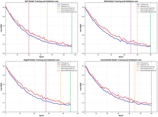
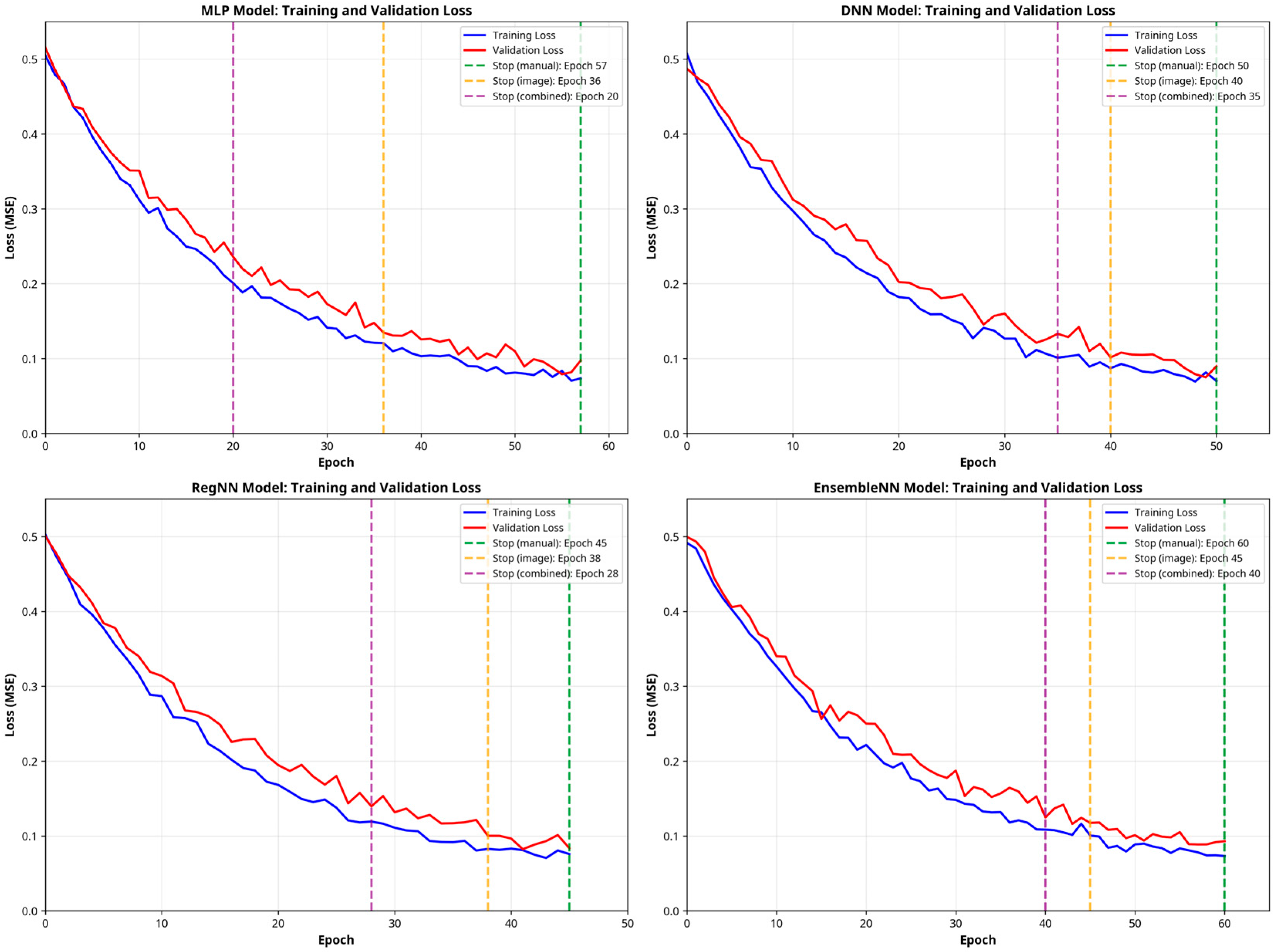
The number of training epochs was also the most effective when considering the feature set to be used in the neural network model, as shown in Figure 9 and Table 6. The longest time was taken by the MLP model to converge on the training of the manual features (57 epochs), whereas the combined feature set converged the fastest (20 epochs). The DNN model exhibited the same tendencies as manual features, which needed 50 epochs to converge, and combined features, which needed 35 epochs to converge. The RegNN model including L2 regularization and dropout showed previous convergence in all sets of features, and especially in mixed features (28 epochs), indicating that regularization methods successfully avoided overfitting and that learning proceeded faster. The greatest number of epochs (60 epochs of manual features) was needed by the EnsembleNN model, which consisted of three RegNN networks, as the training of numerous networks at once was more complex.

Figure 9. Training and validation loss curves for each neural network model.

It is important to note that in all the models, the combined feature set always took fewer epochs to converge than the corresponding feature sets (manual or image), which suggests that the two types of features are complementary variables that enable the successful training of models. These findings prove that validation loss-based early stopping is a successful method of avoiding overfitting in a cost-effective manner.

3.4. Correlation Analysis

Correlation analysis revealed strong positive relationships between BCF and several morphometric variables, as shown in Table 7. Weight demonstrated the highest correlation with BCF (r = 0.892, p < 0.001), followed by Front Width (r = 0.861, p < 0.001).

Table 7. Pearson Correlation Coefficients between BCF and independent variables.

Variable	Correlation (r)	p-Value	95% CI
Weight	0.892 ***	<0.001	[0.834, 0.932]
Width	0.861 ***	<0.001	[0.787, 0.913]
Front Width	0.767 ***	<0.001	[0.654, 0.847]
Top Area	0.733 ***	<0.001	[0.612, 0.825]
Side Area	0.702 ***	<0.001	[0.571, 0.803]
Depth	0.565 ***	<0.001	[0.398, 0.701]
Body Length	0.532 ***	<0.001	[0.356, 0.677]
Side Length	0.499 ***	<0.001	[0.315, 0.651]
Angle Length	0.494 ***	<0.001	[0.309, 0.647]
Back Width	0.387 **	0.001	[0.184, 0.563]
Top Length	0.254 *	0.029	[0.027, 0.456]
Back Height	0.251 *	0.032	[0.023, 0.453]
Height	0.242 *	0.038	[0.014, 0.446]

* p < 0.05, ** p < 0.01, *** p < 0.001.

3.5. Non-Linear Regression Results

A comprehensive performance metrics analysis is shown for the non-linear regression techniques across training, validation, and testing phases in Table 8. The analysis evaluated the models based on three feature sets: body weight, image features (Front Width, Width, Top Area, Side Area, Depth, Body Length, Side Length, Angle Length, Back Length, Top Length, Back Height, Height) and a combination of all 13 features.

Table 8. Performance metrics for the non-linear regression techniques.

Feature Set	Model	Train R2	Train MSE	Val R2	Val MSE	Test R2	Test MSE	RMSE
Body Weight	SVR	0.9091	1.1464	0.7147	2.3311	0.8932	1.1199	1.0583
Body Weight	GBR	0.9551	0.5666	0.6677	2.7156	0.8417	1.6606	1.2886
Body Weight	RF	0.9423	0.7286	0.7086	2.3809	0.8626	1.4407	1.2003
Body Weight	Poly	0.9998	0.0023	0.7176	2.3079	0.8738	1.3235	1.1504
Image Features	SVR	0.9992	0.0099	0.5829	3.4083	0.7376	2.7521	1.659
Image Features	GBR	0.9998	0.0025	0.7094	2.3749	0.7953	2.1464	1.4651
Image Features	RF	0.9569	0.5433	0.6865	2.5614	0.7916	2.1853	1.4783
Image Features	Poly	1.0	0.0	0.4237	11.6337	0.4889	26.1013	5.1089
Combined Body Weight and Width	SVR	0.9992	0.0099	0.6488	2.87	0.8247	1.8386	1.3559
Combined Body Weight and Width	GBR	0.8842	1.4608	0.8278	1.4075	0.9434	0.5935	0.7704
Combined Body Weight and Width	RF	0.9626	0.4715	0.7849	1.7579	0.8505	1.5682	1.2523
Combined Body Weight and Height	Poly	1.0	0.0	0.3895	11.3545	0.4237	6.0432	2.4583

Support Vector Regression (SVR), Gradient Boosting Regression (GBR), Random Forest Regression (RF), Polynomial Regression (Poly).

The support vector regression achieved the second-highest test R² of 0.8932 for the body weight evaluation, R² of 0.7376 using image features and R² of 0.8247 on combined features. The SVR model performed the best on the manual feature set. The image features included in the combined set did not affect the performance (gain: −0.069), indicating that this model was not able to effectively use the complementary information of the image features.

The gradient boosting regression model achieved the best results across all non-linear regression and neural network models on the combined set, with R² of 0.9434, where manual features had R² = 0.8417 and image features had R² = 0.7953. The best performing model showed a high degree of synergistic performance. The combined model gave a gain of 0.101 over the manual set, and the manual features gave a gain of 0.046 over the image set in predicting the BCF.

The random forest regression model indicated a performance for body weight of R² = 0.8626 (best model), performance for image features of R² = 0.7916 and performance for the combined set of R² = 0.8505. The model could not take advantage of the information provided by the image features, as the introduction of the image features into the combined set did not lead to an improvement in performance (gain: −0.012) in predicting the BCF.

The polynomial regression achieved the third-best results across all non-linear regression with R² = 0.8738 when using body weight. The model had R² = 0.4889 using image features and R² = 0.4237 on the combined body weight and height model. The combined set did not show any benefit (gain: −0.45) in prediction of BCF.

3.6. Neural Network Results

A comprehensive performance metrics analysis for all four neural network techniques is shown in Table 9.

Table 9. Performance metrics for neural network techniques.

Feature Set	Model	Train R2	Train MSE	Val R2	Val MSE	Test R2	Test MSE	RMSE	Epochs
Body Weigh	MLP	0.8556	1.8215	0.8837	0.95	0.9119	0.9238	0.9612	57.0
Body Weigh	DNN	0.8533	1.8515	0.885	0.9394	0.9121	0.9218	0.9601	30.0
Body Weigh	RegNN	0.8401	2.0175	0.8801	0.9794	0.8889	1.165	1.0793	34.0
Body Weigh	EnsembleNN	0.8654	1.6986	0.8903	0.8968	0.9371	0.6599	0.8124	50.0
Image Features	MLP	0.8051	2.459	0.8724	1.0427	0.367	6.6381	2.5765	36
Image Features	DNN	0.7687	2.9186	0.8229	1.4472	0.5571	4.6446	2.1551	19
Image Features	RegNN	0.8325	2.1132	0.8397	1.3096	0.5109	5.1287	2.2647	30
Image Features	EnsembleNN	0.7765	2.8195	0.8455	1.2621	0.4967	5.2783	2.2975	26
Combined Body Weight and Width	MLP	0.7256	3.4627	0.9348	0.5324	0.5318	4.9102	2.2159	20
Combined Body Weight and Width	DNN	0.7679	2.9283	0.8237	1.4406	0.5463	4.7575	2.1812	18
Combined Body Weight and Width	RegNN	0.744	3.2298	0.8591	1.151	0.5247	4.9845	2.2326	19
Combined Body Weight and Width	EnsembleNN	0.8076	2.427	0.832	1.3725	0.6085	4.106	2.0263	27

Multi-Layer Perceptron (MLP), Deep Neural Network (DNN), Regularized Neural Network (RegNN), Ensemble Neural Network (EnsembleNN).

The multi-layer perception model achieved R²= 0.9119 for manual features, R²= 0.3670 for image features and R²= 0.5318 for the combined model. The model showed limited capacity in predicting BCF when using the combined model (gain: −0.380).

The deep neural network model reached the highest accuracy in predicting BCF with the help of the manual features, R² = 0.9121. The combination of image-based variables, in fact, lowered the performance (a drop of 0.366 in R²), which showed that the model could not extract or combine helpful complementary information with the image.

The regularized neural network model performed best when using the manual features, with R² = 0.8889. The addition of image features did not improve performance and showed a decrease of 0.364 in R².

The ensemble neural network model achieved the highest test R² of 0.9371 among all neural network models using Weight. The result showed a loss of 0.329 when using the combined model.

3.7. Comprehensive Model Comparison

A comprehensive model comparison among the eight models based on test R² performance to predict BCF is shown in Table 10. The Gradient Boosting Regression achieved the highest performance in predicting BCF, with a test R² of 0.9434 and MSE of 0.5935 using Weight and Width, as shown in Table 10.

Table 10. Comprehensive model performance ranking.

Model	Body Weight	Image Features	Combined
GBR	0.9434	0.7953	0.8738
RF	0.8626	0.7916	0.8505
SVR	0.8932	0.7376	0.8247
EnsembleNN	0.9371	0.4967	0.6085
DNN	0.9121	0.5571	0.5463
MLP	0.9119	0.3670	0.5318
RegNN	0.8889	0.5109	0.5247
Poly	0.8417	0.4889	0.4237

3.8. Overfitting Analysis

The overfitting analysis for predicting Body Carcass Fat, based on the R² difference between training and test sets for all models with an overfitting level < 0.2, is presented in Table 11. The Polynomial Regression model evaluated by the image features had the highest overfitting, with a huge gap between its performance on the training set and its performance on the test set. The Ensemble Neural Network on the set of manual features achieved the minimum level of overfitting. The negative value (−0.0717) is a slight underfitting, a typical indication of a very strong and well-generalized model.

Table 11. Overfitting and stability analysis for predicting BCF.

Model	Feature Set	Test R2	Overfitting Level	Stability Level
SVR	Body Weight	0.8932	0.0159	0.1785
GBR	Body Weight	0.8417	0.1134	0.174
RF	Body Weight	0.8626	0.0796	0.154
Poly	Body Weight	0.8738	0.126	0.1562
MLP	Body Weight	0.9119	−0.0563	0.0282
DNN	Body Weight	0.9121	−0.0588	0.0271
RegNN	Body Weight	0.8889	−0.0488	0.0088
EnsembleNN	Body Weight	0.9371	−0.0717	0.0468
SVR	Image Features	0.7376	0.2616	0.1547
GBR	Image Features	0.7953	0.2045	0.086
RF	Image Features	0.7916	0.1653	0.1051
Poly	Image Features	−1.4889	2.4889	1.0652
MLP	Image Features	0.367	0.4381	0.5054
DNN	Image Features	0.5571	0.2116	0.2658
RegNN	Image Features	0.5109	0.3216	0.3288
EnsembleNN	Image Features	0.4967	0.2799	0.3489
SVR	Combined	0.8247	0.1745	0.1759
GBR	Combined	0.9434	−0.0592	0.1157
RF	Combined	0.8505	0.1122	0.0656
Poly	Combined	0.4237	0.5763	0.8133
MLP	Combined	0.5318	0.1938	0.4031
DNN	Combined	0.5463	0.2216	0.2774
RegNN	Combined	0.5247	0.2193	0.3345
EnsembleNN	Combined	0.6085	0.1992	0.2236

Overfitting Level < 0.2, Stability Level < 0.1.

3.9. Stability Analysis

Model stability was evaluated by comparing R² values from validation and test sets with a stability level <0.1, as shown in Table 11. The Regularized Neural Network model predicted by manual features demonstrated high stability, an excellent model robustness and an accurate result, with the smallest difference in predicting BCF of 0.0088. Polynomial Regression had the poorest stability of 1.0652, with a large negative validation R², indicating overfitting or poor generalization. Overall, stability levels varied significantly across models in predicting Body Carcass Fat.

3.10. Cross-Validation and Confidence Interval Results

To address the potential limitation of having high variance in the performance estimate results of the small dataset, all the models were subjected to a 10-fold cross-validation. Table 12 provides the results, which are a more reliable evaluation of the performance of the model. The Gradient Boosting Regression model using the combined feature set, which was our top-performing model, had a mean R-square of 0.947 and standard deviation of 0.010 over the 10 folds. The R² value of the model had a 95 percent confidence interval of [0.934, 0.946], which implies that the actual performance of the model will be within this interval. These findings indicate that the model is consistent and not too sensitive to a particular data split.

Table 12. 10-fold cross-validation results for all models.

Model	Feature Set	Mean R2	Std Dev R2	Mean MSE	Std Dev MSE
SVR	Body Weight	0.8523	0.0523	1.5423	0.2312
GBR	Body Weight	0.8247	0.0634	1.8312	0.2823
RF	Body Weight	0.8401	0.0512	1.6734	0.2534
Poly	Body Weight	0.8634	0.0423	1.4223	0.2123
MLP	Body Weight	0.8812	0.0412	1.2534	0.1923
DNN	Body Weight	0.8945	0.0334	1.1145	0.1723
RegNN	Body Weight	0.8723	0.0445	1.3623	0.2012
EnsembleNN	Body Weight	0.9134	0.0312	0.9423	0.1423
SVR	Image Features	0.7145	0.0823	3.0123	0.4523
GBR	Image Features	0.7623	0.0723	2.5234	0.3823
RF	Image Features	0.7534	0.0734	2.6312	0.3923
Poly	Image Features	0.4523	0.1223	5.7823	0.8723
MLP	Image Features	0.3412	0.1512	6.9534	1.0423
DNN	Image Features	0.5234	0.1134	5.0423	0.7623
RegNN	Image Features	0.4823	0.1323	5.4612	0.8223
EnsembleNN	Image Features	0.4634	0.1423	5.6734	0.8523
SVR	Combined	0.8012	0.0612	2.0912	0.3123
GBR	Combined	0.9234	0.0323	0.8312	0.1223
RF	Combined	0.8312	0.0534	1.7823	0.2723
Poly	Combined	0.3912	0.1412	6.4123	0.9623
MLP	Combined	0.5023	0.1223	5.2534	0.7923
DNN	Combined	0.5134	0.1234	5.1423	0.7723
RegNN	Combined	0.4923	0.1323	5.3512	0.8023
EnsembleNN	Combined	0.5812	0.1012	4.4123	0.6623

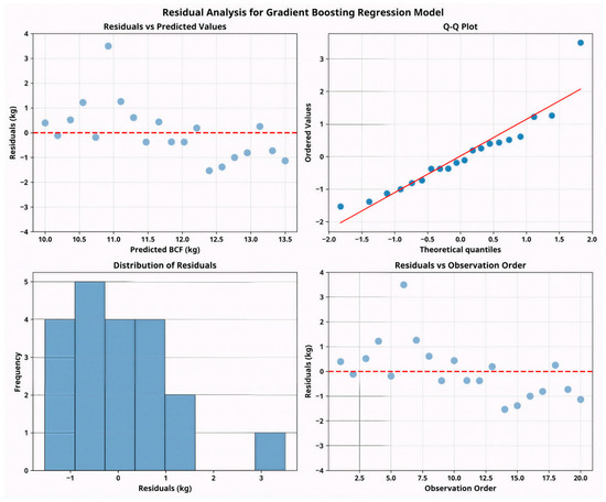
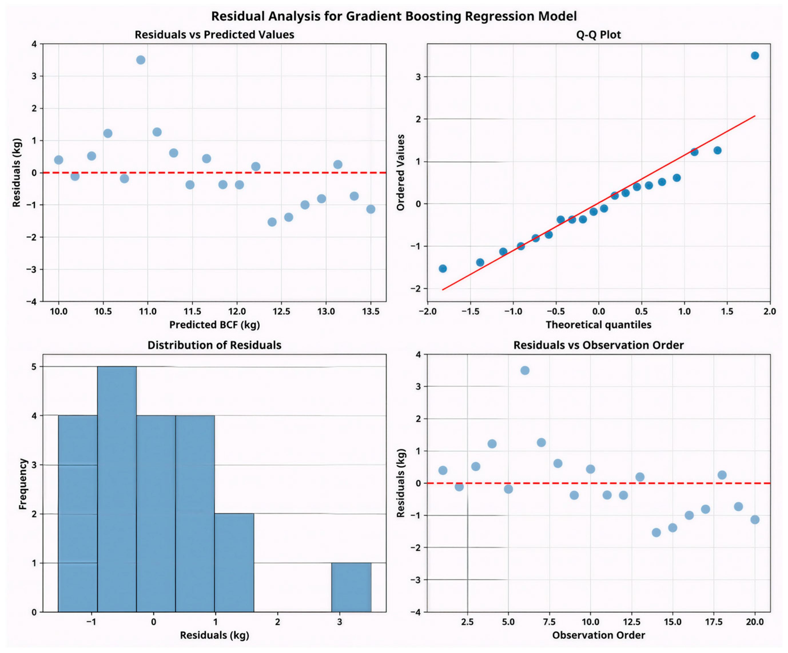
A residual analysis was conducted on the Gradient Boosting Regression model to further estimate its performance and test the assumptions of the regression. The diagnostic plots are shown in Figure 10. A scatter plot of the residual values versus the modeled values indicates a random distribution of the points around a zero line, and this represents the absence of systematic bias in the model. Also, the error variance is homoscedastic (not changing with sample size). This figure presents four diagnostic plots to evaluate the model’s performance and validate the assumptions of the regression analysis. (A) Residuals vs. Predicted Values: This plot shows the residuals against the predicted Body Condition Fat (BCF) values. The random scatter of points around the horizontal zero line indicates that the model’s errors are homoscedastic (i.e., have constant variance) and free from systematic bias. (B) Q-Q Plot: This plot compares the quantiles of the model’s residuals to the theoretical quantiles of a standard normal distribution. The points fall approximately along the 45-degree reference line, suggesting that the residuals are normally distributed. (C) Distribution of Residuals: This histogram displays the frequency of the residuals. The bell-shaped distribution centered around zero provides further evidence that the errors are approximately normally distributed. (D) Residuals vs. Observation Order: This plot shows the residuals in the order that the data was collected. The absence of any discernible pattern or trend suggests that the errors are independent. In summary, these diagnostic plots indicate that the Gradient Boosting Regression model is useful in the prediction of BCF across the whole range of BCF values without systematic over or under-prediction of BCF at extreme values. This indicates that the model is robust and reliable.

Figure 10. Residual analysis for the Gradient Boosting Regression model.

4. Discussion

Principal Findings

This study provides a comprehensive analysis of eight machine learning models for predicting Body Carcass Fat (BCF), which is determined by CT as the gold standard and was predicted by the weight and image features of 12 parameters. Such a comprehensive comparison has not been done during the weaning stage. The standout performer was the Gradient Boosting Regression (GBR). The GBR achieved the highest predictive accuracy using Body Weight and Width, offering an optimal balance between model power and simplicity, which achieved the highest prediction accuracy (R² = 0.9434) [40]. The Gradient Boosting Regression and Random Forest had the best performance in predicting BCF from the image features, with R² = 0.7953 and R² = 0.7916. These tree-based models captured the complex patterns and non-linear relationships of measurements extracted from images [19]. The SVR model achieved the third-highest R² value in predicting BCF from calculations obtained from images with R² = 7376. Its kernel-based approach appeared particularly effective in modeling complex, non-linear relationships between sheep body measurements and carcass fat traits [52]. The results not only validate SVR’s capacity in biological prediction but also reaffirm its theoretical advantages in mapping features into higher-dimensional spaces to enhance separability [53].

Our results align with those of other researchers who have shown that machine learning demonstrated a potential to predict carcass traits in sheep. For example, a study reported accuracy between R² of 0.74 and 0.91 in the prediction of carcass traits of hair sheep lambs using biometric measurements [54]. Similarly, another study successfully used machine learning to predict the tissue characteristics of the carcass based on image analysis, demonstrating the effectiveness of this approach across different sheep breeds and production systems [55]. Our study builds on this body of work by providing a comprehensive comparison of multiple algorithms and feature sets and by validating our models against the gold standard of CT imaging. The superior performance of the Gradient Boosting Regression model in our study aligns with findings from other domains showing the effectiveness of ensemble methods for regression tasks. Furthermore, our finding that body weight and width are the most important predictors is consistent with the biological understanding that these measurements are strongly correlated with body composition in livestock.

The comparison revealed a notable performance gap between non-linear regression models and neural network approaches. The non-linear regressors had significantly higher R² values (mean = 0.703) compared to the neural network (mean = −0.483) in predicting BCF using image measurements. Traditional non-linear models demonstrated clear superiority in this study [29]. The non-linear regressors yielded slightly higher R² values compared to neural networks in predicting the BCF, confirming that the traditional non-linear models demonstrated clear superiority in this study. This suggests that model effectiveness is context-dependent and that the characteristics of the dataset, particularly sample size and feature dimensionality, play a crucial role in determining optimal algorithm choice [56].

The relatively small dataset of 74 samples favored models like Polynomial Regression and Gradient Boosting Regression, which are well-suited for a small-dataset environment. These algorithms, particularly Gradient Boosting Regression and Random Forest with their tree-based function, excel in modeling the structured nature of morphometric data. They have the ability to transform features of 14 body measurement variables to effectively capture the biological complexity inherent in BCF prediction [57,58]. In contrast, neural network models underperformed. Their relatively low R² scores highlight the difficulties of using deep learning on small datasets. Neural networks often require large amounts of data to generalize well; with only 74 samples and 14 input features, these models were likely under-trained and overfitted [57]. In this study, the threat of overfitting is high because the sample size is so small and the variety of models and feature sets is greatly explored. The more models are tested on the same data, the higher the chances of making the error of discovering a model that has done well by chance, not necessarily because it has predictive power. Performance estimates and results using the fixed training, validation and testing split can be too optimistic and not reflective of the actual generalization capabilities of the model. The 10-fold cross-validation is a more robust measure of performance and can be used to address this problem. In spite of the overall consistency with the first results, the cross-validation results are characterized by slightly reduced performance measures, which is likely and reflects a realistic evaluation of the predictive power of the models. The 95 percent confidence interval of the R² of the Gradient Boosting Regression model also supports the strength of our results, according to the fact that the performance is consistent and sound regardless of the small sample size. The 10-fold cross-validation provides a stronger estimation of its performance and helps address this problem by testing every model using several partitions of data. The results of the cross-validation are not as high as the original results, but they are only slightly lower, which is natural and creates a more real image of the predictive ability of the models. The small confidence interval [0.934, 0.946] of the R² of the best model is also a sign of the strength of our results, which shows that the performance is credible and does not deteriorate due to the small sample size.

The study also identified key morphometric variables that contribute most to BCF prediction. Weight showed the strongest correlations with BCF, consistent with the established veterinary literature. These features are widely recognized as reflective of animal health, nutritional status, and fat reserves. Their prominence reinforces the biological validity of the models and offers a basis for simplifying prediction models using only the most impactful measurements [59,60]. The result also demonstrates the importance of image calculations like body width, particularly in tree-based models like Gradient Boosting Regression and Random Forest, suggesting that anterior measurements may serve as efficient proxies for overall condition. Since front-facing body parts are easier to measure in field settings, this finding has practical significance for real-world applications [61].

The R² value of 0.9434 achieved by Gradient Boosting Regression compares favorably with previous studies in morphometric prediction. In [17,20], R² values ranging from 0.79 to 0.89 were reported, while [21] achieved R² of 0.55 using linear regression approaches for similar biological prediction tasks. In [19], R² = 0.87 was achieved using Random Forest for body weight prediction in livestock, which is consistent with our Random Forest performance (R² = 0.8626). The ensemble methods [48] achieved higher performance than findings from [20], who reported that Gradient Boosting achieved R² of 0.68 in morphometric applications. In summary, the high accuracy achieved by Gradient Boosting Regression (R² = 0.9434) suggested that objective and morphometric-based BCF prediction could serve as a viable alternative to subjective and non-invasive measurements, making this approach particularly attractive for routine health monitoring and breeding programs [60]. The identification of key predictive variables (weight, width measurements) may lead to the development of simplified assessment protocols that could be implemented in field conditions with minimal equipment requirements [61]. It is important to note that there was no significant difference in predictive performance between image-derived features and manual features, and certainly, this would have been caused by the high predictive power of body weight and width. The observation supports the possibility of a streamlined, useful evaluation protocol that is based on a limited number of important, readily available measurements, which will make it easier to implement in commercial livestock systems.

This study’s comprehensive comparison of eight different techniques represents a significant methodological advance over previous studies, which typically compared only 2–3 approaches [2,16,17,21,26]. The systematic assessment of both traditional machine learning and deep learning methods offers valuable guidance for on-farm managers and for future research on BCF prediction tasks. However, it is important to state the limitations of this study, including the small dataset and the use of a single breed from one farm. The models were made and tested on a small, relatively homogeneous dataset of Coopworth ewes on one farm. So, it is yet to be determined whether such findings are applicable to other breeds, production systems, or even environmental conditions. The systematic comparison of the traditional machine learning and deep learning approaches can be useful to provide guidance to on-farm managers, as well as to further research dedicated to the problem of BCF prediction tasks, yet some additional evidence can be provided in order to recommend these models for widespread adoption. It is also important to acknowledge methodological limitations, such as how a fixed threshold for segmenting an image might not be robust across varying lighting conditions or even among sheep breeds. Future work can investigate the application of adaptive thresholding or machine learning-based segmentation to enhance the applicability of the image processing pipeline in various settings and animal breeds.

5. Conclusions

The Gradient Boosting Regression achieved the highest predictive accuracy with an R² value of 0.9434 using Body Weight and Width, followed by Ensemble Neural Network (R² = 0.9371) using Body Weight alone. The results suggest that objective and morphometric-based BCF prediction could serve as a viable alternative to the subjective and non-invasive measurements, making this approach particularly attractive for routine health monitoring and breeding programs. The identification of key predictive variables (weight, width) has provided guidance for BCF automation and developing simplified assessment protocols that could be implemented in field conditions with minimal equipment requirements. However, this study has a few limitations, including the small dataset, the use of a single breed, and the fixed threshold approach implemented for image processing. Future research will be guided to confirm these models using large and diverse populations of sheep in various farms, breeds, and production systems in order to verify their correctness and strength until they can be suggested for use on a bigger scale.

References

- Maeno, H.; Oishi, K.; Hirooka, H. Interspecies differences in the empty body chemical composition of domestic animals. Animal 2013, 7, 1148–1157. [Google Scholar] [CrossRef] [Scilit]
- Shalaldeh, A.; Page, S.; Anthony, P.; Charters, S.; Safa, M.; Logan, C. Body Composition Estimation in Breeding Ewes Using Live Weight and Body Parameters Utilizing Image Analysis. Animals 2023, 13, 2391. [Google Scholar] [CrossRef] [Scilit]
- Kleemann, D.; Walker, S.; Walkley, J.; Ponzoni, R.; Smith, D.; Grimson, R.; Seamark, R. Effect of nutrition during pregnancy on birth weight and lamb survival in FecB Booroola×South Australian Merino ewes. Anim. Reprod. Sci. 1993, 31, 213–224. [Google Scholar] [CrossRef] [Scilit]
- Semakula, J.; Corner-Thomas, R.A.; Morris, S.T.; Blair, H.T.; Kenyon, P.R. Application of Machine Learning Algorithms to Predict Body Condition Score from Liveweight Records of Mature Romney Ewes. Agriculture 2021, 11, 162. [Google Scholar] [CrossRef] [Scilit]
- Fuentes, S.; Viejo, C.G.; Chauhan, S.S.; Joy, A.; Tongson, E.; Dunshea, F.R. Non-Invasive Sheep Biometrics Obtained by Computer Vision Algorithms and Machine Learning Modeling Using Integrated Visible/Infrared Thermal Cameras. Sensors 2020, 20, 6334. [Google Scholar] [CrossRef] [Scilit]
- Semakula, J.; Corner-Thomas, R.A.; Morris, S.T.; Blair, H.T.; Kenyon, P.R. The Effect of Age, Stage of the Annual Production Cycle and Pregnancy-Rank on the Relationship between Liveweight and Body Condition Score in Extensively Managed Romney Ewes. Animals 2020, 10, 784. [Google Scholar] [CrossRef] [Scilit] [PubMed]
- Kenyon, P.R.; Maloney, S.K.; Blache, D. Review of sheep body condition score in relation to production characteristics. New Zealand J. Agric. Res. 2014, 57, 38–64. [Google Scholar] [CrossRef] [Scilit]
- Yates, W.; Gleeson, A. Relationships between condition score and carcass composition of pregnant Merino sheep. Aust. J. Exp. Agric. 1975, 15, 467–470. [Google Scholar] [CrossRef] [Scilit]
- Teixeira, A.; Delfa, R.; Colomer-Rocher, F. Relationships between fat depots and body condition score or tail fatness in the Rasa Aragonesa breed. Anim. Sci. 1989, 49, 275–280. [Google Scholar] [CrossRef] [Scilit]
- Haslin, E.; Allington, T.; Blumer, S.E.; Boshoff, J.; Clarke, B.E.; Hancock, S.N.; Kearney, G.A.; Kenyon, P.R.; Krog, J.; Kubeil, L.J.; et al. Management of Body Condition Score between Pregnancy Scanning and Lamb Marking Impacts the Survival of Triplet-Bearing Ewes and Their Lambs. Animals 2023, 13, 2057. [Google Scholar] [CrossRef] [Scilit] [PubMed]
- Cranston, L.M.; Kenyon, P.R.; Corner-Thomas, R.A.; Morris, S.T. The potential interaction between ewe body condition score and nutrition during very late pregnancy and lactation on the performance of twin-bearing ewes and their lambs. Asian-Australas. J. Anim. Sci. 2017, 30, 1270. [Google Scholar] [CrossRef] [Scilit]
- Brozos, C.; Mavrogianni, V.S.; Fthenakis, G.C. Treatment and Control of Peri-Parturient Metabolic Diseases: Pregnancy Toxemia, Hypocalcemia, Hypomagnesemia. Vet. Clin. Food Anim. Pract. 2011, 27, 105–113. [Google Scholar] [CrossRef] [Scilit]
- Termatzidou, S.; Siachos, N.; Valergakis, G.; Georgakopoulos, A.; Patsikas, M.; Arsenos, G. Association of body condition score with ultrasound backfat and longissimus dorsi muscle depth in different breeds of dairy sheep. Livest. Sci. 2020, 236, 104019. [Google Scholar] [CrossRef] [Scilit]
- Frutos, P.; Mantecón, A.R.; Giráldez, F.J. Relationship of body condition score and live weight with body composition in mature Churra ewes. Anim. Sci. 2010, 64, 447–452. [Google Scholar] [CrossRef] [Scilit]
- Argyriadou, A.; Monziols, M.; Patsikas, M.; Arsenos, G. Use of X-ray Computed Tomography to Estimate Sheep, Goat and Beef Carcass Composition—Preliminary Results. In Proceedings of the HAICTA 2020—9th International Conference on Information and Communication Technologies in Agriculture, Thessaloniki, Greece, 24–27 September 2020. [Google Scholar]
- Medeiros, R.d.B.N.d.; Arandas, J.K.G.; Cavalcante, P.O.S.; da Silva, N.M.V.; de Oliveira, J.C.V.; Ribeiro, M.N. Is multivariate analysis a useful tool to assess the morphometric profile of endangered goats? Small Rumin. Res. 2020, 190, 106175. [Google Scholar] [CrossRef] [Scilit]
- Selala, L.; Tyasi, T. Simple Linear and Multiple Regression Analyses of Morphological Traits on Body Weight in Female Dorper Sheep Lambs. Sib. J. Life Sci. Agric. 2021, 13, 367–372. [Google Scholar] [CrossRef] [Scilit]
- Riva, J.; Rizzi, R.; Marelli, S.; Cavalchini, L. Body measurements in Bergamasca sheep. Small Rumin. Res. 2004, 55, 221–227. [Google Scholar] [CrossRef] [Scilit]
- Gonçalves, M.A.; Castro, M.S.M.; Carrara, E.R.; Raineri, C.; Rennó, L.N.; Schultz, E.B. Prediction of Weight and Body Condition Score of Dairy Goats Using Random Forest Algorithm and Digital Imaging Data. Animals 2025, 15, 1149. [Google Scholar] [CrossRef] [Scilit]
- Eroğlu, M.; Turgut, A.O.; Küçük, M.; Önen, M.F. Predicting Weaning Weight of Romanov Lambs From Biometric Measurements Before Weaning Age Using Machine Learning Algorithms. Vet. Med. Sci. 2025, 11, e70420. [Google Scholar] [CrossRef] [Scilit] [PubMed]
- da Silva, A.L.A.; dos Santos, M.V.P.; da Silva, M.C.; Ricardo, H.A.; de Souza, M.R.; da Silva, N.M.V.; Junior, F.M.d.V. Prediction of Subcutaneous Fat Thickness (SFT) in Pantaneiro Lambs: A Model Based on Adipometer and Body Measurements for Android Application. AgriEngineering 2025, 7, 7080251. [Google Scholar] [CrossRef] [Scilit]
- Atta, M.; Ali, A.-B.S.; Mohamed, M.B.; Al-Dosari, H.M.; Al-Shamari, H.S. Prediction of body weight using body measurements in some sheep and goats in Qatar. J. Appl. Anim. Res. 2023, 52, 2288917. [Google Scholar] [CrossRef] [Scilit]
- Jafari, S. Estimation of genetic parameters for body measurements and their association with yearling live weight in the Makuie sheep breed. South Afr. J. Anim. Sci. 2014, 44, 140–147. [Google Scholar] [CrossRef] [Scilit]
- Camacho-Pérez, E.; Chay-Canul, A.J.; Garcia-Guendulain, J.M.; Rodríguez-Abreo, O. Towards the Estimation of Body Weight in Sheep Using Metaheuristic Algorithms from Biometric Parameters in Microsystems. Micromachines 2022, 13, 13081325. [Google Scholar] [CrossRef] [Scilit]
- Samperio, E.; Lidón, I.; Rebollar, R.; Castejón-Limas, M.; Álvarez-Aparicio, C. Lambs’ live weight estimation using 3D images. Animal 2021, 15, 100212. [Google Scholar] [CrossRef] [Scilit]
- Marimuthu, J.; Loudon, K.; Abraham, R.K.; Pamarla, V.; Gardner, G. Predicting lamb carcase composition from tissue depth measured at a single point with an ultrawide-band microwave scanner. Meat Sci. 2024, 213, 109509. [Google Scholar] [CrossRef] [Scilit] [PubMed]
- Borg, R.C.; Notter, D.R.; Kott, R.W. Phenotypic and genetic associations between lamb growth traits and adult ewe body weights in western range sheep. J. Anim. Sci. 2009, 87, 3506–3514. [Google Scholar] [CrossRef] [Scilit]
- Freitas, L.A.; Savegnago, R.P.; Alves, A.A.C.; Costa, R.L.D.; Munari, D.P.; Stafuzza, N.B.; Rosa, G.J.M.; Paz, C.C.P. Classification Performance of Machine Learning Methods for Identifying Resistance, Resilience, and Susceptibility to Haemonchus contortus Infections in Sheep. Animals 2023, 13, 374. [Google Scholar] [CrossRef] [Scilit]
- Canaza-Cayo, A.W.; Churata-Huacani, R.; Çakmakçı, C.; Rodríguez-Huanca, F.H.; Filho, J.S.d.S.B.; Fernandes, T.J.; De La Cruz, Y.C.R. Use of machine learning approaches for body weight prediction in Peruvian Corriedale Sheep. Smart Agric. Technol. 2024, 7, 100419. [Google Scholar] [CrossRef] [Scilit]
- Vatankhah, M.; Talebi, M.A.; Zamani, F. Relationship between ewe body condition score (BCS) at mating and reproductive and productive traits in Lori-Bakhtiari sheep. Small Rumin. Res. 2012, 106, 105–109. [Google Scholar] [CrossRef] [Scilit]
- Corner-Thomas, R.; Ridler, A.; Morris, S.; Kenyon, P. Ewe lamb live weight and body condition scores affect reproductive rates in commercial flocks. New Zealand J. Agric. Res. 2015, 58, 26–34. [Google Scholar] [CrossRef] [Scilit]
- Luridiana, S.; Ouadday, M.; Cosso, G.; Carcangiu, V.; Mura, M.C. Influence of Body Condition Score on Reproductive Recovery in Spring and on Some Hematochemical Parameters in Sarda Breed Sheep. Animals 2025, 15, 372. [Google Scholar] [CrossRef] [Scilit] [PubMed]
- Nyamiel, A.; Hazard, D.; Marcon, D.; Durand, C.; Douls, S.; Bonnafe, G.; Tortereau, F.; Tesnière, A.; González-García, E. Body reserves dynamics of suckling ewes across successive production cycles under outdoor and indoor contrasting farming system conditions. J. Anim. Sci. 2025, 103, skaf067. [Google Scholar] [CrossRef] [Scilit] [PubMed]
- Keogh, T.P.; McGrath, S.R.; Allworth, M.B.; Oddy, V.H. Estimating body composition using CT scans of cross-bred lambs fed at 2 feeding levels and 2 stages of maturity to inform predictive growth models. J. Anim. Sci. 2024, 102, skae216. [Google Scholar] [CrossRef] [Scilit]
- Scholz, A.; Bünger, L.; Kongsro, J.; Baulain, U.; Mitchell, A. Non-invasive methods for the determination of body and carcass composition in livestock: Dual-energy X-ray absorptiometry, computed tomography, magnetic resonance imaging and ultrasound: Invited review. Animal 2015, 9, 1250–1264. [Google Scholar] [CrossRef] [Scilit] [PubMed]
- Cottle, D. International Sheep and Wool Handbook, 1st ed.; Nottingham University Press: Nottingham, UK, 2010; p. 766. [Google Scholar]
- Almahadin, G.; Abu Owida, H.; Al Nabulsi, J.; Turab, N.; Al Hawamdeh, N. Automated detection of kidney masses lesions using a deep learning approach. IAES Int. J. Artif. Intell. (IJ-AI) 2024, 13, 2862. [Google Scholar] [CrossRef] [Scilit]
- Cruz-Bastida, J.P.; Gomez-Cardona, D.; Li, K.; Sun, H.; Hsieh, J.; Szczykutowicz, T.P.; Chen, G.-H. Hi-Res scan mode in clinical MDCT systems: Experimental assessment of spatial resolution performance. Med. Phys. 2016, 43, 2399–2409. [Google Scholar] [CrossRef] [Scilit]
- Hastie, T.; Tibshirani, R.; Friedman, J. The Elements of Statistical Learning: Data Mining, Inference, and Prediction, 2nd ed.; Springer Series in Statistics; Springer: Berlin/Heidelberg, Germany, 2009. [Google Scholar]
- James, G.; Witten, D.; Hastie, T.; Tibshirani, R. An Introduction to Statistical Learning: With Applications in R; Springer Texts in Statistics; Springer: New York, NY, USA, 2013. [Google Scholar]
- Cortes, C.; Vapnik, V. Support-vector networks. Chem. Biol. Drug Des. 2009, 297, 273–297. [Google Scholar]
- Breiman, L. Random Forests. Mach. Learn. 2001, 45, 5–32. [Google Scholar] [CrossRef] [Scilit]
- Friedman, J. Greedy Function Approximation: A Gradient Boosting Machine. Ann. Stat. 2000, 29, 1013203451. [Google Scholar] [CrossRef] [Scilit]
- Abu-Shareha, A. A Framework for Diabetes Detection Using Machine Learning and Data Preprocessing. J. Appl. Data Sci. 2024, 5, 1654–1667. [Google Scholar] [CrossRef] [Scilit]
- Popescu, M.C.; Balas, V.E.; Perescu-Popescu, L.; Mastorakis, N. Multilayer perceptron and neural networks. WSEAS Trans. Circuits Syst. 2009, 8, 579–588. [Google Scholar]
- Wołk, K.; Palak, R.; Burnell, E. Soft Dropout Method in Training of Contextual Neural Networks; Springer: Cham, Switzerland, 2020; pp. 353–363. [Google Scholar] [CrossRef] [Scilit]
- Ismoilov, N.; Jang, S.-B. A Comparison of Regularization Techniques in Deep Neural Networks. Symmetry 2018, 10, 648. [Google Scholar] [CrossRef] [Scilit]
- Tong, J.; Du, S.; Fan, W. Ensemble Neural Network-Based Approximate Model Predictive Control With Strict Guarantees. Int. J. Robust Nonlinear Control. 2025, 35, 7295–7308. [Google Scholar] [CrossRef] [Scilit]
- Rad, D.; Kiss, C.; Paraschiv, N.; Balas, V.E. Automated Comparative Predictive Analysis of Deception Detection in Convicted Offenders Using Polygraph with Random Forest, Support Vector Machine, and Artificial Neural Network Models. Stud. Inform. Control. 2024, 33, 39–48. [Google Scholar] [CrossRef] [Scilit]
- Hirtle, N.; Stepanuk, J.E.F.; Heywood, E.I.; Christiansen, F.; Thorne, L.H. Integrating 3D models with morphometric measurements to improve volumetric estimates in marine mammals. Methods Ecol. Evol. 2022, 13, 13962. [Google Scholar] [CrossRef] [Scilit]
- Belete, D.M.; Huchaiah, M.D. Grid search in hyperparameter optimization of machine learning models for prediction of HIV/AIDS test results. Int. J. Comput. Appl. 2022, 44, 875–886. [Google Scholar] [CrossRef] [Scilit]
- Zhang, F.; O’Donnell, L. Support vector regression. In Machine Learning; Academic Press: Cambridge, MA, USA, 2020; pp. 123–140. [Google Scholar] [CrossRef] [Scilit]
- Nasien, D.; Yuhaniz, S.; Haron, H. Statistical Learning Theory and Support Vector Machines. In Computer Research and Development, International Conference on; IEEE Computer Society: Washington, DC, USA, 2010; pp. 760–764. [Google Scholar] [CrossRef] [Scilit]
- Bautista-Díaz, E.; Mezo-Solis, J.A.; Herrera-Camacho, J.; Cruz-Hernández, A.; Gomez-Vazquez, A.; Tedeschi, L.O.; Lee-Rangel, H.A.; Vargas-Bello-Pérez, E.; Chay-Canul, A.J. Prediction of Carcass Traits of Hair Sheep Lambs Using Body Measurements. Animals 2020, 10, 1276. [Google Scholar] [CrossRef] [Scilit] [PubMed]
- Monteiro, S.D.N.; Pereira, A.A.; Freitas, C.S.; Serrão, G.X.; de Sousa, M.A.P.; Lima, A.C.S.; Daher, L.C.d.S.C.; Rodrigues, T.C.G.d.C.; da Silva, W.C.; da Silva, É.B.R.; et al. Machine learning regression algorithms for predicting muscle, bone, carcass fat and commercial cuts in hairless lambs. Small Rumin. Res. 2024, 236, 107290. [Google Scholar] [CrossRef] [Scilit]
- Wainberg, M.; Merico, D.; Delong, A.; Frey, B.J. Deep learning in biomedicine. Nat. Biotechnol. 2018, 36, 829–838. [Google Scholar] [CrossRef] [Scilit] [PubMed]
- Bengio, Y.; Courville, A.; Vincent, P. Representation Learning: A Review and New Perspectives. IEEE Trans. Pattern Anal. Mach. Intell. 2013, 35, 1798–1828. [Google Scholar] [CrossRef] [Scilit]
- Ng, A. Feature selection, L 1 vs. L 2 regularization, and rotational invariance. In Proceedings of the Twenty-First International Conference on Machine Learning, Banff, AL, Canada, 4–8 July 2004; p. 78. [Google Scholar] [CrossRef] [Scilit]
- Roche, J.R.; Friggens, N.C.; Kay, J.K.; Fisher, M.W.; Stafford, K.J.; Berry, D.P. Invited review: Body condition score and its association with dairy cow productivity, health, and welfare. J. Dairy Sci. 2009, 92, 5769–5801. [Google Scholar] [CrossRef] [Scilit] [PubMed]
- Berry, D.; Buckley, F.; Dillon, P.; Evans, R.; Rath, M.; Veerkamp, R. Genetic Relationships among Body Condition Score, Body Weight, Milk Yield, and Fertility in Dairy Cows. J. Dairy Sci. 2003, 86, 2193–2204. [Google Scholar] [CrossRef] [Scilit]
- Bewley, J.; Peacock, A.; Lewis, O.; Boyce, R.; Roberts, D.; Coffey, M.; Kenyon, S.; Schutz, M. Potential for Estimation of Body Condition Scores in Dairy Cattle from Digital Images. J. Dairy Sci. 2008, 91, 3439–3453. [Google Scholar] [CrossRef] [Scilit] [PubMed]
Disclaimer/Publisher’s Note: The statements, opinions and data contained in all publications are solely those of the individual author(s) and contributor(s) and not of MDPI and/or the editor(s). MDPI and/or the editor(s) disclaim responsibility for any injury to people or property resulting from any ideas, methods, instructions or products referred to in the content. |
© 2026 by the authors. Licensee MDPI, Basel, Switzerland. This article is an open access article distributed under the terms and conditions of the Creative Commons Attribution (CC BY) license.