


Abstract
In light of the dual challenges of global climate change and the pressure on agricultural resources, increasing crop yields and resource utilization efficiency has become the key to ensuring food security and sustainable agricultural development. This study takes environmental factors and cultivation measures as input and crop yield as output; systematically compares five ensemble learning models: RF, LightGBM, GBDT, XGBoost, and CatBoost; and then screens out the CatBoost algorithm with the best performance. The CatBoost-Nondominated Sorting Genetic Algorithm II (NSGA-II) hybrid model was constructed. This model provides data-driven solutions and strategies for cultivating rice and maize through precise yield prediction and multi-objective optimization. To enhance the interpretability of the model, we used the SHAP method to parse the predicted behavior to ensure that the results conform to common agricultural knowledge. Based on this, we constructed a constrained multi-objective optimization problem and solved it using the NSGA-II algorithm to obtain a Pareto frontier that strikes a balance among yield, resource consumption and growth cycle. Case studies showed that CatBoost performs best in the selected datasets. SHAP identified precipitation, fertilization/irrigation intensity and temperature as the main influencing factors; NSGA-II generated a well-distributed Pareto solution set, allowing for the flexible selection of representative cultivation schemes based on different management objectives. This modeling paradigm showed good generalization ability and can be extended to other crop cultivation strategy optimization scenarios based on tabular data.
1. Introduction
Agriculture is a vital sector of the national economy. Its yield performance is intricately tied to national food security and social stability [1,2]. Accurate prediction of grain crop yields holds significant importance in enabling governments to craft effective agricultural policies and provide timely production guidance to enhance agricultural efficiency [3]. Currently, due to intensifying climate change and mounting population pressure, precise prediction and optimization of grain crop yields have become key research priorities in the field of agriculture [4,5]. Traditional crop-planting decisions largely hinge on farmers’ experience and intuition; however, given the need to capture the nonlinear mapping between inputs and outputs, as well as the trade-offs among conflicting multi-objectives, this approach often leads to supply–demand mismatches and wasting of resources, since there are considerable climatic variations across regions and limited agricultural resources [6]. To foster sustainable agricultural development, it is essential to adopt intelligent methods for making informed crop-planting decisions and effective management strategies such as reducing costs in terms of irrigation, fertilization, and planting timing [7].
The yield of grain crops is influenced by many factors, including soil quality, precipitation levels, temperature, fertilization intensity, irrigation extent, and the number of crop growth days, among others [8]. Given that crop yield is subject to the combined constraints of the aforementioned factors, when formulating crop-planting strategies that balance crop yield, planting site selection, and resource consumption, multi-objective conflicts are inevitable. For instance, an exclusive focus on maximizing crop yield will lead to excessive fertilization and irrigation, which results in a certain increase in resource consumption [9]. These issues render the optimization of crop yield a complex challenge [10,11]. At present, cultivation strategy optimization is mainly achieved through field trials and empirical recommendations, statistical/response-surface designs, and process-based crop models or decision-support systems. However, these approaches often become costly and inefficient when the decision space is high-dimensional and strongly nonlinear, and they are difficult to scale to precision agriculture scenarios with heterogeneous soils and climate variability. Therefore, there is a global need for a scalable prediction–evaluation–optimization framework to support cultivation strategy design under resource constraints and climate variability. Hence, an optimization strategy that can comprehensively consider multiple objectives and effectively address complex influencing factors is required. The key to designing such a strategy lies in constructing precise mathematical models for crop yield prediction and multi-objective optimization.
In crop yield prediction, models must integrate multi-source data (e.g., soil conditions, climatic factors, agronomic practices) while capturing complex interactions among these variables [12,13,14]. Accurate predictive models provide reliable inputs and evaluation bases for subsequent multi-objective optimization [15]. Early predictive modeling studies mainly relied on field experimental data and traditional statistical methods, such as structural equation modeling and regression analysis, to establish input–output relationships. French et al. [16] predicted Mediterranean wheat yield based on agrometeorological inputs. Qian et al. [17] employed stepwise regression combined with cross-validation to select predictive variables in a multiple linear regression model for forecasting spring wheat yield from sowing to harvest. Mohamed Emran et al. [18] applied response surface methodology in conjunction with central composite design to predict the optimal water and fertilizer prerequisites for maize cultivation, thereby optimizing water–fertilizer management in sandy soils. Bi et al. [19] utilized structural equation modeling together with field experiments to compare the yield of monocultures and mixtures in order to assess the effects of plant diversity and optimize fertilization schemes and seeding ratios in legume–grass mixed pastures. However, these simple linear regression or statistical models exhibit two core weaknesses in handling complex, high-dimensional agricultural data: inadequate modeling capacity and poor generalization. The former refers to their inability to fully process high-dimensional inputs and capture nonlinear interactions among climate, soil, and management variables; the latter stems from their over-reliance on localized experimental data, which constrains their applicability to diverse real-world scenarios.
In recent years, advances in computer technology and data analysis tools have led researchers to incorporate machine learning methods into crop yield prediction models, including Support Vector Machines, Deep Neural Networks (e.g., Long Short-Term Memory Networks, Convolutional Neural Networks), and Ensemble Learning [20,21,22]. In order to construct a high-precision crop yield prediction model base on RMSE and R2, this study tested five classic ensemble algorithms, namely Random forest (RF), Light Gradient Boosting Machine (LightGBM), gradient boosting decision tree (GBDT), eXtreme Gradient Boosting (XGBoost), and Categorical Boosting (CatBoost). Through the evaluation of fitting ability and generalization performance, the optimal algorithm was selected as the core method [23,24,25]. SHAP (SHapley Additive exPlanations) was used to evaluate the model’s interpretability and verify its coherence [23]. Sustainable agricultural decisions require a balance of yield, costs, resource efficiency, ecological consequences, and forecasting [26,27]. Conventional weighted-sum optimization often neglects the nonlinear trade-offs and is vulnerable to arbitrary parameter choices [2,28]. This research presents a multi-objective optimization framework employing NSGA-II (Nondominated Sorting Genetic Algorithm II), which utilizes Pareto dominance to generate nondominated solution sets without requiring human weight allocation. The resultant Pareto front provides decision-makers with a spectrum of planting tactics, ranging from resource-intensive methods to environmentally focused approaches [29,30]. Against this background, the central question of this study is whether a unified prediction–evaluation–optimization framework can be built on tabular agricultural data to support cultivation strategy design for rice and maize in a way that is both reliable and agronomically interpretable. Specifically, we ask whether a data-driven surrogate can capture the non-linear yield response under coupled climatic and management factors, and whether the resulting surrogate can be coupled with a multi-objective optimizer to generate strategy sets that explicitly reveal trade-offs, rather than relying on a single weighted objective.
Our working hypothesis is that ensemble learning models can serve as a robust surrogate model for yield prediction under mixed-type features, and that SHAP-based evaluation can provide transparent evidence for how key variables and their interactions contribute to yield variation. Building on this, we further hypothesize that integrating the surrogate with NSGA-II enables efficient exploration of the decision space and yields Pareto-efficient cultivation strategies that balance competing goals.
A key gap is the limited availability of cultivation-optimization frameworks that explicitly accommodate crop and zone-specific agro-climatic heterogeneity. Although maize and rice are predominantly produced under distinct climatic regimes and exhibit different global yield baselines, many data-driven studies implicitly assume that a single fixed model or optimization setting can be transferred across production contexts. This motivates a flexible prediction–evaluation–optimization framework that can be retrained and externally validated on region field datasets, so that the learned yield response surface and the resulting Pareto-efficient strategies reflect local agro-climatic conditions and constraints.
This study utilizes machine learning and heuristic optimization algorithms to create a novel integrated “prediction–evaluation–optimization” modeling framework tailored for tabular agricultural datasets, addressing the challenges of accurate food crop yield prediction and multi-objective optimization. We first employ a data-driven approach, utilizing ensemble learning algorithms to construct predictive models. We then interpret and validate the models using SHAP (SHapley Additive exPlanations) interpretability analysis. Finally, we apply multi-objective optimization algorithms to design a planting plan that achieves both high crop yield and low cost. Rice and maize, two of the most crucial food crops around the world, serve as case studies to examine methods for enhancing factors that influence production throughout cultivation. The research analyzes publicly available data from the Kaggle platform, including 13,869 entries on rice production and 13,915 entries on maize cultivation. Six variables (precipitation, temperature, growth duration, fertilizer application, irrigation, and soil quality) are selected as inputs, with yield per hectare as the output. A multi-objective optimization model is developed by integrating genetic algorithms for optimization with the ensemble machine learning for prediction. The new framework encompasses the following key tasks:
- Five ensemble learning models were systematically tested to select the optimal CatBoost model, as it accurately describes the nonlinear relationship between yield per hectare and its influencing factors.
- A comprehensive assessment of the CatBoost model utilizing the SHAP (SHapley Additive exPlanations) approach is performed to ensure its dependable interpretability.
- A multi-objective optimization problem with reasonable constraints, addressed using the Nondominated Sorting Genetic Algorithm II (NSGA-II) is formulated to derive an optimal configuration solution set (Pareto front) that balances multiple objectives, including yield, water consumption, fertilization, and harvest duration.
The core innovation of this study lies in providing a data-driven optimization research solution for the setting of subsequent optimization objectives and the definition of constraint conditions for decision variables, addressing the core issue of “black-box prediction and blind optimization” in traditional optimization models. The methodology and framework we have constructed are highly versatile. After testing and replacing some modules (such as the prediction algorithm), it can be transferred to other agricultural datasets to be used in similar research on increasing yield and reducing costs.
2. Materials and Methods
2.1. Model Framework
This research analyzes rice and maize as crop examples, focusing on two main optimization objectives in agriculture: increasing productivity and reducing resource use. It presents a novel integrated modeling approach for “prediction–evaluation–optimization”, as illustrated in Figure 1. The research methodology progresses through three phases. A high-precision predictive model is constructed using contemporary agricultural statistics to correlate soil attributes, meteorological patterns, and cultivation techniques with crop yield. Secondly, the SHAP method is employed to conduct interpretability analysis of the model, precisely identifying key influencing factors and providing a solid theoretical foundation for the rational setting of subsequent optimization objectives. Finally, based on the established prediction model, multiple objective functions, including yield and resource consumption, are incorporated into the optimization framework, and the NSGA-II is utilized for multi-objective optimization to obtain the Pareto optimal solution set.
Figure 1.
The model framework of the “prediction—evaluation—optimization” strategy.
The proposed framework is data-agnostic and can be instantiated with different agricultural datasets. The demonstration dataset used in this study serves to illustrate the end-to-end workflow. Field deployment would rely on retraining and validation using region field records. Yield can be approximated as a function of the recorded environmental and management variables at the dataset resolution. SHAP provides attribution-based (non-causal) explanations for model evaluation, and NSGA-II searches Pareto-efficient solutions within an explicitly bounded mixed discrete–continuous decision space.
2.2. Data Collection and Preprocessing
In this study, through agriculture data extraction and screening of the Kaggle website (https://www.kaggle.com/datasets/samuelotiattakorah/agriculture-crop-yield) (accessed on 1 June 2025), we obtained a “rice planting environment yield” dataset comprising 13,869 records and a “maize planting environment-yield” dataset with 13,915 records. Each record in these datasets contains six input feature variables: the six input features describe the environmental factors in rice cultivation, including rainfall (Rainfall_mm), temperature (Temperature_Celsius), growth duration (Days_to_harvest), fertilizer application (Fertilizer_Used), irrigation (Irrigation_Used), and soil type (Soil_Type). The output feature is the crop yield per hectare (Yield_tons_per_hectare). During the training process of the prediction model, the data were divided into training and testing sets in an 8:2 ratio.
Because the benchmark dataset does not provide explicit geographic metadata, we do not interpret the learned relationships as representing any specific global production zone; instead, the dataset is used to demonstrate the proposed workflow, while field deployment would rely on retraining and external validation using region records.
2.3. Dataset Description
Since the dataset does not provide the actual amounts of fertilizer applied and irrigation conducted, but instead uses 0 to indicate that fertilizer or irrigation was used and 1 to denote implementation, for the sake of general applicability, it can be assumed that the dataset considers the degree of on-demand execution for fertilization/irrigation. Specifically, a value of 1 indicates that fertilization/irrigation was fully carried out in accordance with actual agricultural requirements, and values within the interval (0, 1) are used to represent partial implementation, i.e., only a certain proportion of the recommended fertilizer or irrigation level is applied. Soil type is a categorical variable, with 0 meaning Peaty (peat soil), 1 representing Clay (clayey soil), 2 representing Silt (silty soil), 3 representing Loam (loam soil), 4 meaning Chalky (chalky soil), and 5 representing Sandy (sandy soil). The number of days to harvest is an integer variable, while the remaining variables are numerical. The correlation degrees among the numerical variables and their respective distributions are illustrated in Figure 2 and Figure 3.
Figure 2.
Correlation between variables and distribution of numerical variables in rice dataset: (a) correlation between variables; (b) distribution of numerical variables.
Figure 3.
Correlation between variables and distribution of numerical variables in maize dataset: (a) correlation between variables; (b) distribution of numerical variables.
The numerical variable characteristics of the dataset were analyzed. Table 1 shows the descriptive statistical results. Overall, the growth environments of rice and corn share certain similarities, but they also show key differences. The annual average precipitation for rice is 554.2 mm, whereas for maize, it is slightly lower at 549.0 mm. The rainfall amounts for both crops exhibit considerable fluctuation, with standard deviations of 259.0 mm and 258.0 mm, respectively. The temperature difference between the two is minor; the temperature of the rice is 27.5 °C and that of maize is 27.4 °C. Both crops exhibit temperature variations ranging from 15.0 °C to 40.0 °C, with standard deviations of 7.2 °C and 7.3 °C, respectively. Regarding the growth cycle, both crops mature within a range of 60 to 149 days and have minimal variation. Rice yields have minimal variation, which is characterized by a standard deviation of 1.7 tons per hectare. It has a standard variation of 5.9 tons per hectare. This indicates that maize yields are influenced by a greater number of factors, resulting in more significant variations.
Table 1.
Descriptive statistics of numerical variables for rice and maize.
The descriptive statistical results of the categorical variables of rice and corn are shown in Table 2. In the cultivation of rice and corn, the application of fertilizers and irrigation is comparable. Approximately fifty percent of the samples do not utilize either option. The soil-type distribution is approximately uniform for both rice and maize; each of the six categories (Silt, Clay, Peaty, Chalky, Sandy, and Loam) accounts for roughly 16–18% of the samples.
Table 2.
Descriptive statistics of categorical variables for rice and maize.
Analysis of variance shows that irrigation and fertilization factors have a certain impact on crop yield, whereas the categorical variable “soil type” exerts a relatively minor influence. This is clearly observable from the distributions depicted in the two box plots in Figure 4: on the horizontal axis, the shapes and positions of the yield box plots corresponding to different soil types are strikingly similar.
Figure 4.
Box plot of soil types vs. numerical variables: (a) rice; (b) maize.
Although temperature, harvest days, and soil type do not exert a decisive influence on yield compared to other variables, they have not been overlooked in this study. On the one hand, since the dimensionality of the model inputs is not high, these factors are included as part of the predictive inputs to enhance prediction accuracy. On the other hand, in the results of subsequent optimizations, the optimized temperature and soil type hold guiding significance for planting site selection, while harvest days are also beneficial for designing cost-effective planting schemes.
This study’s dataset shows no data bias. To mitigate potential imbalance in the benchmark setting, we adopted a stratified splitting strategy and reported cross-validation results. For potential bias in other datasets, one can use stratified sampling for sampling bias, cross-annotation for annotation bias, and standardized tools for measurement bias.
2.4. Construction of the Prediction Model
2.4.1. Ensemble Learning Methods
To achieve accurate prediction of crop yields, this study conducts modeling analysis using multiple ensemble learning algorithms based on the screened database. Given that crop yields are subject to nonlinear and coupled influences from multiple factors, five mainstream gradient boosting-based ensemble learning algorithms are selected for comparative research in this paper, namely Random Forest (RF), Light Gradient Boosting Machine (LightGBM), Gradient Boosting Decision Tree (GBDT), eXtreme Gradient Boosting (XGBoost), and Categorical Boosting (CatBoost). These algorithms demonstrate excellent predictive performance when handling high-dimensional, nonlinear data with complex interactions among features. They have been widely applied in various fields, such as agriculture, environmental science, and resource optimization.
Random forest (RF) is an ensemble learning model [31]. Its core idea is to enhance the model’s performance and generalization ability by constructing a large number of decision trees and aggregating their prediction results (voting method for classification tasks and averaging method for regression tasks). This model simultaneously introduces the dual randomness of samples and features during the training process, thereby enhancing the diversity of base learners and effectively suppressing overfitting. Random forests can handle high-dimensional data, assess feature importance, and exhibit robustness to missing values and outliers.
Light Gradient Boosting Machine (LightGBM) is a boosting algorithm that calculates the residuals of the current tree using the first and second-order negative gradients of the loss function to fit new trees [32]. It employs an enhanced histogram technique and a leaf-wise growth strategy with a maximum depth constraint, resulting in improved software performance.
Friedman publicly released the Gradient Boosting Decision Tree (GBDT) algorithm in 1999 [33]. It uses decision trees as fundamental learners and subsequently constructs new decision trees by identifying the residuals of the preceding tree and using them as the target variable. It subsequently rectifies each erroneous output independently. This process continues until either the number of decision trees reaches a predefined maximum or the cumulative residual error falls below a predefined tolerance.
EXtreme Gradient Boosting (XGBoost) is an efficient gradient boosting decision tree approach that enhances model accuracy through the aggregation of several trees [34]. It employs regularization terms to enhance the model’s generalization capacity and other techniques to expedite computations. It performs well on large datasets, allowing for fast parallel processing of data, and can effectively reduce overfitting.
Categorical Boosting (CatBoost) is an algorithm based on gradient boosting decision trees, which inherits the additive modeling and forward stagewise optimization concepts from GBDT [35]. It is particularly well-suited for handling categorical features, since it incorporates ordered boosting technology and automatically handles categorical features. By efficiently preprocessing and encoding categorical data, CatBoost avoids the data leakage issues present in traditional methods, enhances model stability, and is applicable to small-sample datasets, effectively preventing overfitting. From a model architecture perspective, the model constructed by each decision tree can be represented as follows:
Here, = contains all the feature values of the i-th sample (the variable order follows the introduction in Section 2.2), represents the number of trees, and denotes the -th decision tree. Let be the training error for a single sample. The loss function is defined as
In each training round of this method, a new decision tree is generated based on the existing model, following the direction of negative gradient descent of the loss function. It is then incorporated into the overall model, with the learning rate serving as the weight. The formula is as follows:
where represents the newly generated tree in the current round and denotes the learning rate.
The CatBoost model can be used to predict agricultural yields, evaluate the importance of planting factors, and develop crop growth models [24]. It can also be applied to analyze how various environmental factors and management strategies influence crop yield in a nonlinear manner. This provides accurate predictive assistance for the upcoming optimization work [25]. We have listed the pseudocode of the algorithm in Appendix A.
2.4.2. Hyperparameter Tuning Based on Bayesian Optimization
This study implements Bayesian hyperparameter optimization using the Optuna framework [36,37], with its core being the Tree-structured Parzen Estimator (TPE) algorithm. This algorithm fits the mapping relationship between hyperparameters and the model performance objective function through a probabilistic model, and its core logic is based on Bayesian posterior probability update:
where denotes the evaluated hyperparameter-performance sample set, represents the posterior distribution of hyperparameters, and is the prior distribution of the objective function. The TPE algorithm separates the hyperparameter distributions of “excellent performance” () and “ordinary performance” () (denoted as and respectively) and selects the next hyperparameter to be evaluated using the Expected Improvement (EI) criterion:
Here, is the current optimal performance value, and measures the expectation of performance improvement brought by hyperparameter .
The yield prediction models for rice and maize were developed using five distinct algorithms: RF, LightGBM, GBDT, XGBoost, and CatBoost. To ensure optimal generalization performance, each algorithm was tuned by the above Bayesian optimization method with a unique set of hyperparameters specific to the crop dataset, as detailed in Table 3.
Table 3.
Hyperparameter settings for prediction models.
After benchmarking five ensemble-learning algorithms (RF, LightGBM, GBDT, XGBoost, and CatBoost) on both the rice and maize datasets, CatBoost achieved the best overall predictive accuracy and generalization performance. Therefore, CatBoost was selected as the core yield-prediction model for the subsequent SHAP interpretation and multi-objective optimization. As summarized in Table 4, CatBoost delivered stable results under five-fold cross-validation, with R2 = 0.9061 ± 0.0055 for rice and 0.9044 ± 0.0028 for maize, accompanied by low prediction errors (RMSE = 0.5280 ± 0.0063 for rice and 0.5242 ± 0.0062 for maize; MAE = 0.4196 ± 0.0707 for rice and 0.4192 ± 0.0068 for maize). Consistent with the cross-validation results, the hold-out evaluation further confirmed the model’s robustness, yielding test R2 values of 0.9070 (rice) and 0.9047 (maize), with corresponding test RMSE values of 0.5184 and 0.5342, respectively. The small gap between training and test performance indicates limited overfitting and supports the reliability of CatBoost for yield prediction in both crops.
Table 4.
CatBoost performance for rice and maize yield prediction (5-fold CV and hold-out test).
2.4.3. Evaluation Metrics
The optimal model in this study was identified through a comparative performance analysis of nonlinear regression ensemble learning models. The selection was based on two key evaluation metrics: the root mean square error (RMSE) and the coefficient of determination (R2), the mean absolute error (MAE), and the mean absolute percentage error (MAPE), as defined in Equations (4)–(7).
Here, n is the total number of records in the dataset, is the true value of the -th record, is the predicted value for the -th record, and denotes the average of the true values for n records.
After completing the training and construction of predictive models, it is necessary to conduct a systematic comparison of the generalization ability and actual predictive performance of each model. This further verifies the applicability and superiority of the models, with the aim of selecting the algorithm that is most suitable for predicting rice and maize yields.
2.5. SHAP: SHapley Additive exPlanations
SHAP is a popular method for evaluating the interpretability of machine learning models. It uses game theory to assess the significance of each attribute. This approach uses Shapley values as a mathematical framework to analyze the impact of each input feature on the predictions generated by machine learning models. The main concept of its computation is to enumerate all possible feature combinations for each attribute. It then determines how the inclusion or exclusion of that feature affects the output of the model. The SHAP value for the feature is determined by calculating a weighted average of these minor effects. This analytical method can effectively demonstrate the individual impact of each attribute on the expected outcomes.
For each feature in a machine learning model, its Shapley value can be defined by the following formula:
where represents the universal set of features and is a subset of features, with . In the formula, denotes the output of the model trained on the feature subset , and represents the output of the model after incorporating the feature into the subset . The fraction value in the formula reflects the fairness in accounting for different feature-ordering sequences when calculating the Shapley values. For each feature, the SHAP value quantifies its importance by calculating a weighted average of the differences between the model’s output when the feature is included and when it is excluded, across all possible feature subsets .
Interpretability Analysis of Predictive Models
Based on the feature importance ranking derived from the SHAP interpretability analysis depicted in Figure 5, the top four factors influencing rice yield and maize yield, in descending order, are: precipitation, fertilization, irrigation, and temperature, with the remaining factors being harvest days and soil type. The underlying influence mechanisms are as follows: When precipitation values are higher (depicted in red), the SHAP values are larger positive values, indicating that high precipitation significantly boosts yields, whereas low precipitation (depicted in blue) exerts a negative impact on yields. Regarding fertilization amount and irrigation intensity: when these values are high (depicted in red), the SHAP values are positive, suggesting that high levels of fertilization/irrigation enhance yields, whereas low levels of fertilization/irrigation (depicted in blue) tend to decrease predicted yields. For temperature, moderate-to-high values (depicted in red-purple) result in positive SHAP values, promoting yields positively, while low temperature values (depicted in blue) have a negative effect on yields.
Figure 5.
Ranking chart of feature importance for yield: (a) rice; (b) maize.
The terms “high” and “low” are defined relative to the observed range of each feature in the dataset. Taking precipitation in the rice dataset as an example, the observed range is approximately 100–1000 mm (Table 1); values below about 550 mm are regarded as relatively low, whereas values above about 550 mm are regarded as relatively high. In the SHAP dependence plots, the color gradient encodes this information: points corresponding to feature values near the lower bound of the range are displayed in blue, while those near the upper bound are displayed in red. For the binary management variables Fertilizer_Used and Irrigation_Used, 0 (no application) is shown in blue and 1 (full application) in red.
The ranking of feature importance in the predictive model revealed through SHAP interpretability analysis is highly consistent with existing research findings and agricultural experience. Nitrogen fertilizer is important to produce the highest corn output, yet other variables, including weather and soil conditions, may limit productivity [38,39]. Precipitation is one of the key elements that affect maize productivity. A proper amount of rainfall satisfies the maize hydration needs and aids with the process of photosynthesis and absorption of mineral elements [37]. This validation enhances the model’s predictive credibility and scientific accuracy, thereby strengthening the practical significance of our findings for agriculture. We further conducted a detailed analysis of the SHAP dependence plots. As shown in Figure 6 for rice, the horizontal axis denotes the feature value, while the left vertical axis represents the corresponding SHAP value. A higher absolute SHAP value indicates a greater influence on the target variable (yield), with positive/negative signs denoting facilitative or inhibitory effects, respectively. The right vertical axis and the color gradient (from blue for low to red for high) represent the value of an interacting feature (e.g., Fertilizer_Used). The SHAP dependence plots for maize (Figure 7) exhibit similar patterns to those of rice.
Figure 6.
SHAP dependence plots for rice cultivation characteristics.
Figure 7.
SHAP dependence plots for maize cultivation characteristics.
Rising rainfall consistently corresponds to higher SHAP values, confirming its positive role in rice yield formation, which is consistent with established agronomic knowledge. Furthermore, the minimal influence of the color gradient (fertilizer) on this trend implies that the effect of precipitation is robust and not significantly modulated by fertilizer levels. Nevertheless, the maximum SHAP values occur under high rainfall and high fertilizer conditions, suggesting that there may be a weak synergistic effect of “water + fertilizer” in promoting growth. When temperatures range from 20 to 30 °C, higher rainfall corresponds to positive SHAP values, whereas lower rainfall results in more volatile SHAP values, indicating that temperature and rainfall jointly shape the predictive contribution to yield. For harvest periods of 60–100 days, high rainfall is associated with positive SHAP values; however, when harvest duration exceeds 120 days, high rainfall shifts to negative SHAP values, signifying that rainfall’s impact on yield is dependent on harvest cycle length. Additionally, the distribution of fertilizer’s SHAP values differs across soil types, demonstrating that soil type modulates the magnitude of fertilizer’s effect on yield.
As the temperature increases from low to high (within the range of 20–40 °C), the SHAP value increases continuously and monotonically. This means that higher temperatures significantly drive the model’s positive predictions (elevated temperatures are beneficial for crop physiological activity and improve predicted yield/growth status). Temperature is a critical factor for crop growth, and within an appropriate range (excluding extreme heat), increased temperatures enhance physiological processes such as photosynthesis and metabolic rates, aligning with the increasing trend in SHAP values and reflecting the model’s capture of the “temperature promotes growth” pattern.
Lower execution levels of irrigation or fertilization correspond to negative SHAP values, indicating that they adversely affect rice growth and yield. Conversely, higher execution levels result in positive SHAP values, confirming their beneficial effect. This positive impact aligns with agronomic principles, wherein adequate water and nutrient supply is essential for optimal crop performance. The weak influence of the color-coded interacting feature, evidenced by the absence of a clear distribution pattern, suggests that the effect of irrigation/fertilization is robust and operates largely independently of other variables in this context.
Within the growth period range of 80–120 days, the SHAP values are densely clustered, indicating relatively stable impacts of harvest days on yield within this interval (the model judges this range as the conventional growth period for rice, with more consistent impact patterns). Both SHAP values fluctuate greatly for the growth period 60–80 days (short growth period) and 120–140 days (long growth period). It means that effect of extreme growth periods, short or long, on yield is much more complicated and depends on other factors, e.g., precipitation.
It is not certain that soil type has a monotonic effect on prediction results. SHAP values of individual soil codes are spread around the zero axis, and this shows that soil type has a different impact on prediction results depending on other variables.
When temperatures range from 20 to 30 °C, higher rainfall corresponds to positive SHAP values, whereas lower rainfall results in more volatile SHAP values, indicating that temperature and rainfall jointly shape the predictive contribution to yield. For harvest periods of 60–100 days, high rainfall is associated with positive SHAP values; however, when harvest duration exceeds 120 days, high rainfall shifts to negative SHAP values, signifying that rainfall’s impact on yield is dependent on harvest cycle length. Additionally, the distribution of fertilizer’s SHAP values differs across soil types, demonstrating that soil type modulates the magnitude of fertilizer’s effect on yield.
The validation via SHAP dependence plots enhances the assessment of the suggested model’s performance from multiple perspectives, rendering the conclusions more credible and beneficial.
2.6. NSGA-II for Multi-Objective Optimization
To effectively solve multi-objective optimization problems, it is necessary to employ a suitable optimization algorithm, namely Nondominated Sorting Genetic Algorithm II (NSGA-II). As a classic multi-objective genetic algorithm, NSGA-II excels at addressing complex optimization problems involving two or more conflicting objectives [40,41,42]. This method is a fast nondominated sorting-based multi-objective genetic algorithm that conducts searches in an inherently parallel manner through the evolution of a population, representing the entire solution set. A single run can yield a Pareto front composed of multiple preference-free solutions. Its mechanisms of nondominated sorting and crowding distance calculation effectively preserve the diversity and convergence of the solution set [30,40]. In the context of crop planting optimization, this algorithm has been validated to identify the optimal planting structure or management plan that balances multiple objectives, such as economic benefits, water resource utilization efficiency, and greenhouse gas emissions reduction [43,44]. The pseudocode of NSGA-II is shown in the Appendix A.
Figure 8 illustrates the flowchart for the NSGA-II algorithm. The optimization variables, objective functions, and constraints are firstly input. Then it establishes an initial population, specifies the maximum number of iterations G, and initializes the current iteration count to G = 0. Subsequently, nondominated sorting and crowding distance calculation are performed to evaluate individuals in the group. After that, selection, crossover, and mutation operations are performed to generate new offspring populations. These offspring individuals combine with the parent population to form a new group. This process continues until the best solution is found. The basic premise of the genetic algorithm is to use selection, crossover, and mutation to promote the evolution of the population, thereby gradually approaching the optimal answer through iterative enhancement.
Figure 8.
Flowchart of the NSGA-II algorithm.
3. Results and Discussion
3.1. Evaluation and Comparison of Predictive Model Performance
The predictive performance of the five ensemble algorithms on the rice dataset is summarized in Table 5. In terms of R2, GBDT and CatBoost showed the best performance on the training set, while CatBoost outperformed all others on the test set. Regarding RMSE, GBDT achieved the best training set results, whereas CatBoost excelled on the test set.
Table 5.
Comparison of model performance in predicting rice yield.
For the maize dataset, concerning the yield per hectare, the evaluation of the predictive performance of the five ensemble algorithms adopted in this paper is shown in Table 6. In the table, judging by the metric R2, the GBDT and CatBoost algorithms perform best on the training set, while CatBoost outperforms the others on the test set, with the remaining four algorithms showing relatively consistent performance. From the perspective of the RMSE metric, GBDT exhibits the best performance on the training set, whereas CatBoost stands out on the test set. In terms of the metrics MAE and MAPE, CatBoost also demonstrates certain advantages on the dataset.
Table 6.
Comparison of model performance in predicting maize yield.
Figure 9 provides a more intuitive visualization of the predictive performance of the CatBoost algorithm for rice and maize yields. The x-axis represents the actual yield values, while the y-axis shows the corresponding predicted yield values generated by the CatBoost algorithm. Training set samples are depicted as blue dots and test set samples are represented by green dots. For both the training and test sets, the scatter points cluster tightly around the 1:1 line, indicating good agreement between predicted and observed yields. Consistent with this visual impression, CatBoost achieves R2 values of 0.921 and 0.906 on the training and test sets for rice (RMSE = 0.481 and 0.513 t ha−1, respectively), and 0.923 and 0.905 for maize (RMSE = 0.478 and 0.515 t ha−1, respectively) (Table 4 and Table 5) and competitive test MAE (0.407) and MAPE (0.115). Therefore, CatBoost was selected as the core predictive model in the subsequent optimization analysis.
Figure 9.
Performance visualization of CatBoost in predicting yield: (a) rice; (b) maize.
3.2. Multi-Objective Optimization of Optimal Planting Schemes
Objective Function
The CatBoost model shows better prediction accuracy and stability in both the training and testing stages, based on previous results. Consequently, it has been selected as the main predictive instrument for the optimization research in this work. After identifying the key factors and their interrelations, this research proceeds to examine the optimization of scientific cropping patterns with numerous objectives, including better yield, water conservation, and effective fertilization.
The main purpose of this study is to maximize agricultural productivity. The analysis examines irrigation from two perspectives: improving its implementation efficiency and reducing irrigation water use to conserve limited water resources, while shortening the growth cycle to maximize crop rotation and decrease climatic risks. These objectives are inherently interdependent and mutually restrictive: to boost yield, higher irrigation implementation efficiency, fertilization implementation efficiency, and a longer reproductive period are generally necessary. Under water-saving conditions, yield may be notably constrained, and if the aim is to shorten the reproductive period, crop plants may not reach full maturity, resulting in a decline in the final yield. This issue exemplifies a typical multi-objective conflict decision-making problem.
Unlike single-objective optimization problems, multi-objective optimization problems are characterized by the presence of trade-offs among the objective functions, making it impossible to achieve optimal solutions for all objectives simultaneously through a single optimization process [45,46]. To avoid the subjective influence of artificial weighting on the results, this paper constructs a multi-objective optimization model.
In the optimization, we handle soil type as a categorical variable, with the aim of identifying suitable soil cultivation environments. Given that rainfall, as a natural factor that generally cannot be artificially controlled, is not suitable to be used as an optimization variable. This study sets rainfall at fixed values of 300 mm, 600 mm, and 900 mm during the optimization process, corresponding, respectively, to arid, semi-humid, and humid regions (these values can also be adjusted according to specific needs, or rainfall can be included as an optimization variable for refining planting site selection). The optimized soil quality and temperature parameters are then employed as criteria for optimizing planting site selection on a regional basis. The optimization goal is to devise a crop-planting scheme that maximizes yield per hectare while minimizing resource consumption (irrigation and fertilization) and growth duration. The formulas are as follows:
In this study, the objective function for yield is selected as the trained CatBoost regression model, which serves as part of the fitness function for the subsequent NSGA-II algorithm. This approach enables an accurate depiction of the complex nonlinear relationships between input variables and output objectives, thereby enhancing the accuracy of the optimization results.
3.3. Constraint Conditions
In multi-objective optimization, it is crucial to describe constraints to ensure that the optimization results are practical and beneficial to agriculture. Constraints not only illustrate the limitations of resource and management requirements in actual production, but also link the optimization model with the actual production system.
The study utilized the rice- and maize-planting datasets to ascertain the observed ranges (minimum and maximum values) of the continuous variables (rainfall_mm, temperature, harvest_day). The results serve as constraint bounds, as illustrated in Table 7. This choice is reasonable because the dataset values accurately represent the actual environmental conditions and management procedures for planting and harvesting in the study area. Their range of values can truly reflect the feasible planting range in the region, ensuring that the solutions sought in the optimization process have practical production significance and preventing the optimization results from losing their application value due to differences from real conditions.
Table 7.
Value constraint conditions for variables.
For the categorical variable “Soil_Type,” its constraint conditions are directly determined based on the existing soil type categories in the dataset. This is because the classification of soil types is determined by the soil physicochemical properties of the study area, representing a finite set of objectively existing categories. During the optimization process, it is only necessary to screen and select appropriate soil types from within the existing range of soil types, without the need to additionally expand the constraint scope.
3.4. Multi-Objective Optimization Planting Strategies for Rice/Maize
In this study, we investigate how different combinations of management inputs affect production outcomes in rice and maize (specifically yield per hectare, irrigation and fertilization intensity, and growth duration), by performing multi-objective optimization of agricultural output under varying precipitation conditions. Three typical rainfall scenarios are considered: (a) 300 mm, representing arid regions such as rainfed deserts; (b) 600 mm, typical of semi-humid regions; and (c) 900 mm, characteristic of humid regions. By designing these distinct precipitation gradients corresponding to different climatic zones, this study explicitly incorporates regional differences into the optimization framework to reflect context-specific agricultural management needs. These scenarios reflect real-world contexts in which crop production is influenced by natural precipitation—a critical agricultural resource that affects irrigation demand, fertilizer efficacy, and ultimately the selection of cultivation systems.
In arid regions with 300 mm of rainfall, the primary constraint is water scarcity; optimization efforts should therefore focus on balancing irrigation water conservation with yield maintenance. In semi-humid regions receiving 600 mm of precipitation, rainfall and irrigation can function synergistically; thus, optimizing the timing of fertilizer application and irrigation becomes essential. In contrast, in humid regions with 900 mm of rainfall, where water is abundant, the emphasis should shift toward minimizing resource waste and reducing environmental impacts caused by excessive fertilizer use.
This study develops an integrated optimization model to identify suitable rice and maize cultivation methods under specific water constraints, thereby providing regionally tailored management strategies for agricultural production across different climatic zones. Multi-objective optimization aims to identify solutions that simultaneously satisfy multiple competing objectives, resulting in a set of “optimal solutions” that represent the best possible trade-offs. Some candidate solutions are inferior to others across all objectives, a situation referred to as “complete domination.” An example of such a case would be a scenario exhibiting multiple drawbacks, including lower yield, higher irrigation and fertilization intensity, and a longer growth cycle. These inefficient solutions are excluded from consideration. The remaining solutions demonstrate varying performance across different objectives and cannot be evaluated by a single criterion. Together, they form the Pareto front, where no solution is superior to another in all objectives simultaneously. The Pareto front thus represents a balanced solution space in the presence of conflicting goals. In this study, the NSGA-II algorithm is employed to solve the multi-objective optimization model for agricultural yield, thereby generating the Pareto front.
3.4.1. Four-Objective Optimization of Rice Cultivation Plan
Multi-objective optimization seeks a set of “optimal solutions” that satisfy all conflicting objectives while also fulfilling the imposed constraints. Some potential solutions are worse than other potential solutions for all objectives. This is called “total domination.” This situation represents four types of problems: yield reduction, irrigation amount increases, fertilization demand increases, and increasing stay leaf period. These alternatives are not available to us. All the methods show different performances for different objectives, so they cannot be evaluated by a unique criterion. The set of solutions forms the Pareto front solution set. No solution in the Pareto front is superior to another solution for all objectives simultaneously. The Pareto front shows that a balanced combination of alternatives exists in conflicting objectives. In this study, the NSGA-II approach used for the multiple-objective mathematical model of multi-objective optimization of agricultural yield has been applied.
For agricultural practices, each nondominated solution within the Pareto solution set can be regarded as a viable planting strategy. Farmers or agricultural managers can select the planting configuration scheme that best aligns with their practical needs based on their own resource conditions (such as water supply and fertilizer input capacity) as well as their priority objectives (such as higher output or lower resource consumption). The gradient solution points marked in Figure 10 represent the finally selected optimal solution set, which typically balances various objectives in a representative manner.
Figure 10.
Pareto front of four objectives in rice cases: (a) 300 mm; (b) 600 mm; (c) 900 mm.
As shown in Table 8, some typical solutions selected from the Pareto solution set obtained through multi-objective optimization are presented. In the context of multi-objective optimization for rice planting, schemes can be flexibly chosen according to different needs and regional precipitation conditions. Taking arid regions with a precipitation of 300 mm as an example, if the focus is on water conservation, the scheme at Point B can be selected. Characterized by a low irrigation implementation level and a moderate fertilization implementation level, this scheme may not achieve maximum yield but can strike a good balance between resource constraints and production returns. If maximizing yield is the core objective, setting both irrigation and fertilization implementation levels at a high level, corresponding to Point A in the table, can achieve a breakthrough in peak yield. In scenarios of extreme resource scarcity (no watering and no fertilization), Point C provides a basic survival-oriented scheme that ensures the minimum production threshold. When applied to humid regions with a precipitation of 900 mm, other demand dimensions such as fertilizer resource conservation can be prioritized, and similar scheme points like A, B, and C that cater to different needs can also be selected from the Pareto solution set. In addition to focusing on yield, irrigation implementation level, and fertilization implementation level, crop planting locations can be recommended based on different temperatures and soil types within the solution set.
Table 8.
Selection of pareto solution for rice multi-objective optimization.
From the summary in Table 7, the following conclusions can also be drawn:
- (1)
- In arid regions with a precipitation of 300 mm, when both the implementation levels of irrigation and fertilization reach 50%, plots with soil types 2 and 3 can achieve relatively high yields (5.73 and 4.99, respectively). However, as the implementation level of irrigation decreases (e.g., from 50% to 19.5% and then to 0%), yields show a significant declining trend (5.73 → 4.66 → 2.95), reflecting the crucial supporting role of irrigation on yields under arid conditions.
- (2)
- In semi-arid and semi-humid regions with a precipitation of 600 mm, plots with soil types 0 and 2 demonstrate better adaptability. Specifically, when the implementation levels of fertilization (51.2%) and irrigation (53.4%) remain around 50% for soil type 0, the yield can reach 6.83 (the highest in this region). Conversely, when the implementation levels of fertilization or irrigation drop to 0, yields decline significantly (e.g., 4.21 and 4.14). This indicates that a certain level of resource input is required to ensure yields in this region.
- (3)
- In humid regions with a precipitation of 900 mm, soil types 0, 2, 3, 4, and 5 can all achieve relatively high yields. When the implementation levels of fertilization and irrigation are maintained at around 50% and the harvest days are 60, yields generally peak within the range of 8.21 to 8.62. However, if the input of any resource is interrupted (e.g., the implementation levels of fertilization or irrigation are 0) or the harvest days are extended (e.g., to 71 days), yields decrease significantly (ranging from 5.26 to 6.74). This highlights the importance of coordinated resource input and growth period control for high yields under humid conditions.
Despite differences in other conditions, there is an overall trend of significant yield increase with increasing precipitation (the highest yield at 300 mm is 5.73 → the highest at 600 mm is 6.83 → the highest at 900 mm is 8.62), reflecting the fundamental supporting role of natural precipitation in rice production. The results regarding temperature and soil quality can provide support for “regional site selection” and “planting decision-making” in production management.
3.4.2. Four-Objective Optimization of Maize Cultivation Plan
The proposed optimization approach is equally applicable to the optimal design of crop cultivation, such as maize planting. As shown in Figure 11, the obtained Pareto front solution set for maize comprehensively reflects, in the objective space, the trade-off relationships among the four core objectives in planting: “yield, number of harvest days, degree of irrigation implementation, and degree of fertilization implementation.” The interpretation of the corresponding results is similar to that in the case of rice. Suitable planting plans are also selected based on three different rainfall scenarios: 300 mm, 600 mm, and 900 mm.
Figure 11.
Pareto front of four objectives in maize case: (a) 300 mm; (b) 600 mm; (c) 900 mm.
Table 9 presents a selection of representative solutions from the Pareto set for the multi-objective optimization of maize cultivation. These solutions provide adaptable strategies tailored to different precipitation levels and management priorities, such as yield maximization (Point A), balanced resource use (Point B), or minimal input subsistence (Point C). The results demonstrate the model’s capability to support informed decision-making for maize production across diverse climatic conditions.
Table 9.
Selection of pareto solution for maize multi-objective optimization.
It can be summarized from Table 8 as follows:
- (a)
- In arid regions with a precipitation of 300 mm, when the implementation rates of fertilization and irrigation are both maintained at around 50% (53.3%-53.8%), the soil type is 1, and the harvest duration is 62 days, the yield can reach 5.58 (the highest in this region). As the irrigation implementation rate decreases (e.g., from 53.8% to 12.4% and then to 0%) or the harvest duration is extended (e.g., 62 days → 110 days → 147 days), the yield continuously declines (5.58 → 4.17 → 3.79). Moreover, plots with soil type 5 generally have lower yields than those with soil type 1 under the same input conditions, indicating that irrigation assurance and an appropriate growth period (60–62 days) are crucial for high yields under arid conditions, and soil type 1 is more suitable for arid environments.
- (b)
- In semi-arid and semi-humid regions with a precipitation of 600 mm, when soil type 1 receives coordinated inputs of fertilization (50.1%) and irrigation (81.3%) with a harvest duration of 62 days, the yield reaches 7.02 (the highest in this region). Soil type 0 shows a secondary performance with a yield of 6.53 under moderate resource inputs (50.3% fertilization and 54.6% irrigation). However, when the fertilization implementation rate drops to 0, even with a certain level of irrigation maintained (44.8%-53.2%), the yield still significantly decreases (5.46 → 4.59). This suggests that maintaining an appropriate level of fertilization to match the moisture conditions is necessary in this region, and soil types 1 and 0 are more suitable.
- (c)
- In humid regions with a precipitation of 900 mm, when soil type 0 receives balanced inputs of fertilization (50.6%) and irrigation (54.6%) with a harvest duration of 62 days, the yield reaches 8.78 (the highest in this region). Even with a relatively high irrigation implementation rate (59%) but insufficient fertilization (14.5%), or with adequate fertilization (50.9%) but a shortage of irrigation (13.1%), the yields are significantly reduced (7.37 and 7.23, respectively). When resource inputs are completely interrupted (both fertilization and irrigation are 0%), the yield drops to 5.83. This indicates that coordinated resource inputs are the core for high yields under humid conditions, soil type 0 is the most suitable, and a stable growth period of 60–62 days makes it easier to achieve high yields.
Overall, as precipitation increases, the yield shows a stepwise increase (highest yield of 5.58 at 300 mm → highest yield of 7.02 at 600 mm → highest yield of 8.78 at 900 mm). The fundamental supporting role of natural precipitation is remarkable, and all regions exhibit a common pattern for high yields: “coordinated resource inputs + an appropriate growth period”.
The “trade-off” relationship in rice and maize planting plans verifies the essence of multi-objective optimization problems—that the objective functions cannot simultaneously achieve theoretical optimality. The NSGA-II algorithm effectively captures these mutually constrained optimal solutions through nondominated sorting, forming a Pareto front, and providing a scientific space for scheme selection in agricultural production decision-making. Through the above methods, we can get the corresponding solutions satisfying different planting demands and the corresponding planting plan with high yield, less land occupation, and less environmental pollution. Compared with the traditional design method of planting plan, the number of field trials is greatly reduced, and working efficiency is improved. Meanwhile, the above solution provides a reference for the multi-objective optimization design of planting for rice and maize.
Taken together, the above results form a consistent answer to the study’s central aim of building an end-to-end “prediction–evaluation–optimization” pipeline for cultivation strategy design. The comparative evaluation shows that an ensemble learner can provide a stable surrogate for mapping mixed agro-environmental variables to yield, establishing a reliable basis for decision support. Building on this surrogate, the SHAP analysis moves beyond reporting accuracy by revealing how key drivers contribute to the predicted yield response under different precipitation conditions, thereby improving the transparency and interpretability of the modeling step. Finally, the NSGA-II stage operationalizes these learned relationships into a set of Pareto-efficient cultivation strategies, making the trade-offs among yield, management intensity (fertilization/irrigation), and growth duration explicit rather than embedding them in a single weighted objective. In this way, the proposed hybrid framework does not aim to provide a universal “one-size-fits-all” prescription from a single benchmark dataset; instead, it provides a transferable workflow that can be instantiated with region field records through retraining and validation, so that the learned response surface and the resulting strategy set reflect local agro-climatic conditions and practical constraints.
3.5. Limitations and Future Work
This study presents a proof-of-concept implementation of a prediction–evaluation–optimization framework and therefore has several limitations. First, the benchmark dataset does not provide explicit geographic and temporal metadata, and key agronomic factors such as cultivar information, soil physicochemical properties, pest pressure, and management details are not recorded. As a result, the learned surrogate should be interpreted within the data-supported domain, and the reported patterns should not be read as zone-specific causal conclusions. Second, some management variables are encoded in simplified forms in the benchmark data (e.g., binary indicators), and the optimization stage generalizes them to bounded decision variables for scenario exploration; consequently, the Pareto-efficient strategies represent model-implied trade-offs and require empirical validation before being treated as field-ready prescriptions. Third, although the framework is designed to support decision-making under multiple objectives, region-dependent economic factors (e.g., land costs, water pricing) and long-term dynamics (e.g., climate change and soil degradation) are not explicitly modeled in the present benchmark setting.
Future research will instantiate the same framework on multi-year, region-labeled field datasets to assess external validity and transferability across agro-climatic zones. This includes integrating richer agronomic descriptors (e.g., cultivar, soil properties, and management rates), incorporating biologically and regionally plausible constraints in the optimization stage, and conducting uncertainty-aware optimization by propagating predictive uncertainty into the Pareto search. Moreover, controlled field trials can be used to validate candidate strategies from the Pareto front and to calibrate the surrogate model, thereby improving the practical utility of the proposed prediction–evaluation–optimization workflow.
4. Conclusions
This study set out to examine whether a unified prediction–evaluation–optimization framework can be built on tabular agricultural data to support cultivation strategy design for rice and maize in a manner that is both reliable and agronomically interpretable. The results provide consistent evidence that this goal can be achieved within the scope of the benchmark setting. Accordingly, we implemented a hybrid CatBoost–NSGA-II workflow as an end-to-end “prediction–evaluation–optimization” pipeline for crop-yield prediction and cultivation strategy optimization for both rice and maize.
Specifically, environmental conditions and management practices were used as input features, while yield was treated as the target variable. We first conducted a comprehensive comparison of multiple ensemble learning models and identified CatBoost as the most suitable predictor for subsequent interpretation and optimization.
Secondly, the SHAP method is employed to comprehensively evaluate the selected model, ensuring its reliable interpretability. The alignment between the model and agricultural principles, as well as its consistency with existing research findings, has been verified.
Finally, a multi-objective optimization problem is constructed under reasonable constraints and solved using NSGA-II, thereby obtaining a Pareto front that balances multiple objectives such as yield, resource consumption, and harvest days.
The proposed “prediction–evaluation–optimization” research framework exhibits excellent generality and can be widely applied to other crop-planting strategy optimization scenarios based on tabular data. Given that the research in this paper is purely data-driven, when the tabular data contains richer information, our modeling and optimization framework can output planting solutions that better align with agricultural cultivation practices. Subsequent research will build upon this framework to explore more complex agricultural prediction and optimization problems.
Due to the high cost and long duration of field experiments, this study did not include field validation. Future work will focus on enhancing the model’s validation by incorporating regional field trial data, integrating regional disparities in land costs, water prices and long-term dynamic factors (such as climate change and soil degradation) into the current model, and evaluating the transferability and uncertainty of the model framework.
Author Contributions
Conceptualization, Y.Z. and X.X.; methodology, Y.Z.; software, W.Z. and X.X.; validation, A.A.K. and X.X.; formal analysis, X.X.; investigation, Y.Z.; resources, X.X.; data curation, Y.Z.; writing—original draft preparation, Y.Z. and X.X.; writing—review and editing, A.A.K.; visualization, X.X.; supervision, A.A.K.; project administration, X.X.; funding acquisition, Y.Z. All authors have read and agreed to the published version of the manuscript.
Funding
This work is supported by the Tianshan Talent Training Program (No. 2023TSYC-QNTJ0015).
Data Availability Statement
The dataset used in this study can be found in Kaggle. The website is as follows: https://www.kaggle.com/datasets/samuelotiattakorah/agriculture-crop-yield (accessed on 1 June 2025). All codes generated during the study are also all available on request from the author.
Acknowledgments
The authors would like to thank the editors and referees for their valuable comments and suggestions, which helped us to improve the results of this paper.
Conflicts of Interest
The authors declare no conflicts of interest.
Appendix A. Pseudocodes of CatBoost and NSGA-II
Appendix A.1. Pseudocode for CatBoost (Classification/Regression)
- Input:
trainSet: Training set, denoted as {(xi, yi)} (i = 1, 2, …, n; xi: feature vector, yi: target value)
catFeatures: Set of categorical feature indices, denoted as {c1, c2, …, cₖ}
numIterations: Number of boosting iterations, denoted as T
learningRate: Step size for parameter updates, denoted as η
treeDepth: Maximum depth of each decision tree, denoted as d
- Output:
ensembleModel: Trained CatBoost ensemble model M
- Initialization:
1. Categorical feature encoding (Ordered Target Encoding) 1 //Note 1
For each catFeat in catFeatures:
Sort trainSet by target value yi
Compute cumulative mean for each category of catFeat (add prior term λ to avoid overfitting)
Generate encodingMap[catFeat]: mapping from category to numerical value
2. Numerical conversion
Replace all categorical features in trainSet with encoded values via encodingMap → numTrainSet
3. Model initialization
ensembleModel ← Empty set (stores all base decision trees)
residuals ← Initialize residual vector:
residuals[i] = yi (for regression tasks)
residuals[i] = log(yi/(1 − yi)) (for binary classification tasks, log odds)
- For iter in 1 to numIterations:
//Step 1: Build the iter-th symmetric decision tree 2 //Note 2
baseTree ← Construct symmetric decision tree on numTrainSet using current residuals:
Splitting Criterion:
Minimize symmetric Gini coefficient (for classification)
Minimize squared error (for regression)
Regularization: Adopt Ordered Boosting strategy to reduce gradient bias
Constraint: Tree depth ≤ treeDepth
//Step 2: Update model and residuals
treePred ← Prediction values of baseTree on numTrainSet
ensembleModel ← ensembleModel ∪ {baseTree} //Add current base tree to ensemble
residuals ← residuals—learningRate × treePred //Update residuals
- Return ensembleModel
- //Prediction Phase 3 //Note 3
- Function predict (testSample):
//Encode categorical features in test sample
for each catFeat in catFeatures:
testSample[catFeat] ← encodingMap[catFeat][testSample[catFeat]]
//Ensemble prediction
totalPred ← 0
for each baseTree in ensembleModel:
totalPred ← totalPred + learningRate × baseTree.predict (testSample)
//Output result based on task type
if taskType == “regression”:
return totalPred
else if taskType == “classification”:
return sigmoid (totalPred) //Sigmoid activation for binary classification
- Notes for CatBoost pseudocode:
- 1 Ordered Target Encoding: Avoids overfitting by incorporating prior distribution of target values, a core advantage of CatBoost in handling categorical features.
- 2 Symmetric Decision Tree: Ensures balanced tree structure to reduce overfitting risk.
- 3 Prediction Consistency: Maintains the same encoding logic as the training phase to ensure prediction accuracy.
Appendix A.2. Pseudocode for NSGA-II (Multi-Objective Optimization)
- Input:
decisionSpace: Feasible space of decision variables, denoted as Ω
objFunctions: Set of objective functions, denoted as {f1, f2, …, fₘ} (m ≥ 2)
popSize: Size of population in each iteration, denoted as N
maxIterations: Maximum number of evolutionary iterations, denoted as G
- Output:
paretoOptSet: Pareto optimal solution set P
- Initialization:
1. Generate initial population
initPopulation ← Randomly generate N individuals within decisionSpace (each individual is a decision vector)
2. Evaluate initial population 4 //Note 4
For each individual in initPopulation:
individual.objVals ← [f1 (individual), f2 (individual), …, fₘ (individual)]
3. Fast nondominated sorting and crowding distance calculation
[nonDominatedLayers, rankList, crowdingDistList] ← fastNonDominatedSort(initPopulation)
//Assign rank and crowding distance to each individual
for i in 1 to popSize:
initPopulation[i].rank ← rankList[i]
initPopulation[i].crowdingDist ← crowdingDistList[i]
currentPopulation ← initPopulation
- For gen in 1 to maxIterations:
//Step 1: Selection operation 5 //Note 5
parentPopulation ← tournamentSelection (currentPopulation, popSize)
//Step 2: Genetic operations (crossover and mutation)
offspringPopulation ← empty set
for i in 1 to popSize step 2:
parent1 ← parentPopulation[i]
parent2 ← parentPopulation[i + 1]
//Simulated Binary Crossover (SBX)
child1, child2 ← sbxCrossover (parent1, parent2)
//Polynomial Mutation
child1 ← polynomialMutation (child1)
child2 ← polynomialMutation (child2)
offspringPopulation ← offspringPopulation ∪ {child1, child2}
//Step 3: Merge parent and offspring populations
mergedPopulation ← currentPopulation ∪ offspringPopulation (size = 2N)
//Step 4: Evaluate merged population
for each individual in mergedPopulation:
individual.objVals ← [f1 (individual), f2 (individual), …, fₘ (individual)]
//Step 5: Fast non-dominated sorting
[nonDominatedLayers, rankList, crowdingDistList] ← fastNonDominatedSort (mergedPopulation)
//Step 6: Construct next-generation population 6 //Note 6
nextPopulation ← empty set
layerIdx ← 1
while len(nextPopulation) + len(nonDominatedLayers[layerIdx]) ≤ popSize:
nextPopulation ← nextPopulation ∪ nonDominatedLayers[layerIdx]
layerIdx ← layerIdx + 1
//Select remaining individuals from the current non-dominated layer by crowding distance
remainingNum ← popSize—len(nextPopulation)
sortedLayer ← sort(nonDominatedLayers[layerIdx], key = lambda x: x.crowdingDist, reverse = True)
nextPopulation ← nextPopulation ∪ sortedLayer [0:remainingNum]
//Update current population
currentPopulation ← nextPopulation
- //Extract Pareto optimal solutions (rank = 1)
- paretoOptSet ← [ind for ind in currentPopulation if ind.rank == 1]
- Return paretoOptSet
- //Core Function 1: Fast Non-Dominated Sort 7 //Note 7
- Function fastNonDominatedSort (population):
numIndividuals ← len (population)
dominationCount ← [0] × numIndividuals //nₚ: Number of individuals dominating individual p
dominatedSet ← [empty set] × numIndividuals //Sₚ: Set of individuals dominated by individual p
nonDominatedLayers ← empty list //F1, F2, …, Fₖ: Non-dominated layers
//Initialize for each individual
for p in 0 to numIndividuals-1:
for q in 0 to numIndividuals-1:
if p != q:
if dominates(population[p], population[q]):
dominatedSet[p].add(q)
elif dominates(population[q], population[p]):
dominationCount[p] += 1
//Individuals with no dominators belong to the first non-dominated layer
if dominationCount[p] == 0:
population[p].rank ← 1
add population[p] to nonDominatedLayers [0]
//Generate subsequent non-dominated layers
layerIdx ← 0
while len(nonDominatedLayers[layerIdx]) > 0:
tempLayer ← empty set
for p in nonDominatedLayers[layerIdx]:
for q in dominatedSet[p]:
dominationCount[q] -= 1
if dominationCount[q] == 0:
population[q].rank ← layerIdx + 2
add population[q] to tempLayer
layerIdx ← layerIdx + 1
add tempLayer to nonDominatedLayers
//Calculate crowding distance for each individual
crowdingDistList ← crowdingDistanceCalculation(population, nonDominatedLayers)
return [nonDominatedLayers, [ind.rank for ind in population], crowdingDistList]
- //Core Function 2: Crowding Distance Calculation 8 //Note 8
- Function crowdingDistanceCalculation(population, nonDominatedLayers):
crowdingDistList ← [0.0] × len(population)
for layer in nonDominatedLayers:
if len(layer) == 0:
continue
//Calculate crowding distance for each objective function
numObjs ← len(population [0].objVals)
for objIdx in 0 to numObjs-1:
//Sort layer by objective value
sortedLayer ← sort(layer, key = lambda x: x.objVals[objIdx])
//Boundary individuals have infinite crowding distance (prioritize retention)
sortedLayer [0].crowdingDist ← float(‘inf’)
sortedLayer[−1].crowdingDist ← float(‘inf’)
//Calculate crowding distance for middle individuals
objMax ← max([ind.objVals[objIdx] for ind in sortedLayer])
objMin ← min([ind.objVals[objIdx] for ind in sortedLayer])
for i in 1 to len(sortedLayer)-2:
delta ← (sortedLayer[i + 1].objVals[objIdx]—sortedLayer[i − 1].objVals[objIdx])/(objMax—objMin + 1e-6)
sortedLayer[i].crowdingDist += delta
//Assign crowding distance to population
for ind in layer:
idx ← population.index(ind)
crowdingDistList[idx] ← ind.crowdingDist
return crowdingDistList
- Notes for NSGA-II pseudocode:
- 4 Evaluation Consistency: All individuals are evaluated using the same set of objective functions to ensure fairness.
- 5 Tournament Selection: Selects parents based on Pareto rank (primary criterion) and crowding distance (secondary criterion) to maintain population diversity.
- 6 Elitism Preservation: Merges parent and offspring populations to retain high-quality individuals, a core advantage of NSGA-II.
- 7 Fast Non-Dominated Sort: Reduces time complexity of non-dominated sorting, improving algorithm efficiency.
- 8 Crowding Distance: Measures individual density in the objective space to maintain population diversity and avoid local optima.
Table A1.
Information on Python tool libraries.
References
- Godfray, H.C.; Beddington, J.R.; Crute, I.R.; Haddad, L.; Lawrence, D.; Muir, J.F.; Pretty, J.; Robinson, S.; Thomas, S.M.; Toulmin, C. Food security: The challenge of feeding 9 billion people. Science 2010, 327, 812–818. [Google Scholar] [CrossRef] [Scilit] [PubMed]
- Tzachor, A.; Devare, M.; King, B.; Avin, S.; Ó hÉigeartaigh, S. Responsible artificial intelligence in agriculture requires systemic understanding of risks and externalities. Nat. Mach. Intell. 2022, 4, 104–109. [Google Scholar] [CrossRef] [Scilit]
- Sharma, R.K.; Kaur, J.; Feng, G.; Huang, Y.; Kumar, C.; Wang, Y.; Sharma, S.; Jenkins, J.; Dhillon, J. Maize and soybean yield prediction using machine learning methods: A systematic literature review. Discov. Agric. 2025, 3, 64. [Google Scholar] [CrossRef] [Scilit]
- Srivastava, A.K.; Safaei, N.; Khaki, S.; Lopez, G.; Zeng, W.; Ewert, F.; Gaiser, T.; Rahimi, J. Winter wheat yield prediction using convolutional neural networks from environmental and phenological data. Sci. Rep. 2022, 12, 3215. [Google Scholar] [CrossRef] [Scilit]
- Blesh, J.; Hoey, L.; Jones, A.D.; Friedmann, H.; Perfecto, I. Development pathways toward “zero hunger”. World Dev. 2019, 118, 1–14. [Google Scholar] [CrossRef] [Scilit]
- Zhao, J.; Yang, X. Distribution of high-yield and high-yield-stability zones for maize yield potential in the main growing regions in China. Agric. For. Meteorol. 2018, 248, 511–517. [Google Scholar] [CrossRef] [Scilit]
- Saleem, M.H.; Potgieter, J.; Arif, K.M. Automation in Agriculture by Machine and Deep Learning Techniques: A Review of Recent Developments. Precis. Agric. 2021, 22, 2053–2091. [Google Scholar] [CrossRef] [Scilit]
- Khan, A.A.; Wang, Y.-F.; Akbar, R.; Alhoqail, W.A. Mechanistic insights and future perspectives of drought stress management in staple crops. Front. Plant Sci. 2025, 16, 1547452. [Google Scholar] [CrossRef] [Scilit]
- Rahman, K.A.; Zhang, D. Effects of fertilizer broadcasting on the excessive use of inorganic fertilizers and environmental sustainability. Sustainability 2018, 10, 759. [Google Scholar] [CrossRef] [Scilit]
- Groot, J.C.; Oomen, G.J.; Rossing, W.A. Multi-objective optimization and design of farming systems. Agric. Syst. 2012, 110, 63–77. [Google Scholar] [CrossRef] [Scilit]
- Jägermeyr, J.; Müller, C.; Ruane, A.C.; Elliott, J.; Balkovic, J.; Castillo, O.; Faye, B.; Foster, I.; Folberth, C.; Franke, J.A.; et al. Climate impacts on global agriculture emerge earlier in new generation of climate and crop models. Nat. Food 2021, 2, 873–885. [Google Scholar] [CrossRef] [Scilit] [PubMed]
- Arshad, S.; Kazmi, J.H.; Javed, M.G.; Mohammed, S. Applicability of machine learning techniques in predicting wheat yield based on remote sensing and climate data in Pakistan, South Asia. Eur. J. Agron. 2023, 147, 126837. [Google Scholar] [CrossRef] [Scilit]
- Zare, H.; Weber, T.K.D.; Ingwersen, J.; Nowak, W.; Gayler, S.; Streck, T. Within-season crop yield prediction by a multi-model ensemble with integrated data assimilation. Field Crops Res. 2024, 308, 109293. [Google Scholar] [CrossRef] [Scilit]
- Shah, F.; Wu, W. Soil and Crop Management Strategies to Ensure Higher Crop Productivity within Sustainable Environments. Sustainability 2019, 11, 1485. [Google Scholar] [CrossRef] [Scilit]
- Miao, L.; Zou, Y.; Cui, X.; Kattel, G.R.; Shang, Y.; Zhu, J. Predicting China’s Maize Yield Using Multi-Source Datasets and Machine Learning Algorithms. Remote Sens. 2024, 16, 2417. [Google Scholar] [CrossRef] [Scilit]
- French, R.J.; Schultz, J.E. Water use efficiency of wheat in a Mediterranean-type environment. I. The relation between yield, water use and climate. Aust. J. Agric. Res. 1984, 35, 743–764. [Google Scholar] [CrossRef] [Scilit]
- Qian, B.; De Jong, R.; Warren, R.; Chipanshi, A.; Hill, H. Statistical spring wheat yield forecasting for the Canadian prairie provinces. Agric. For. Meteorol. 2009, 149, 1022–1031. [Google Scholar] [CrossRef] [Scilit]
- Emran, M.; El-Gamal, E.H.; Haddad, A.M.; Ibrahim, O.M. Response Surface Methodology for Optimizing Water and Fertilizer Requirements for Maize (Zea mays L.) Growth in Sandy Soil. J. Soil Sci. Plant Nutr. 2024, 24, 6349–6364. [Google Scholar] [CrossRef] [Scilit]
- Bi, Y.; Yang, G.; Wei, Y.; Wilson, G.W.; Wei, B.; He, Y.; Yu, H.; Liu, N.; Zhang, Y. Low legume-grass seeding ratio combined with phosphorus fertilization promotes forage yield and soil quality in managed grasslands. Agron. Sustain. Dev. 2024, 44, 36. [Google Scholar] [CrossRef] [Scilit]
- Chlingaryan, A.; Sukkarieh, S.; Whelan, B. Machine learning approaches for crop yield prediction and nitrogen status estimation in precision agriculture: A review. Comput. Electron. Agric. 2018, 151, 61–69. [Google Scholar] [CrossRef] [Scilit]
- Rashid, M.; Bari, B.S.; Yusup, Y.; Kamaruddin, M.A.; Khan, N. A comprehensive review of crop yield prediction using machine learning approaches with special emphasis on palm oil yield prediction. IEEE Access 2021, 9, 63406–63439. [Google Scholar] [CrossRef] [Scilit]
- Sarker, I.H. Machine learning: Algorithms, real-world applications and research directions. SN Comput. Sci. 2021, 2, 160. [Google Scholar] [CrossRef] [Scilit] [PubMed]
- Hancock, J.T.; Khoshgoftaar, T.M. CatBoost for big data: An interdisciplinary review. J. Big Data 2020, 7, 94. [Google Scholar] [CrossRef] [Scilit] [PubMed]
- Mahesh, P.; Soundrapandiyan, R. Yield prediction for crops by gradient-based algorithms. PLoS ONE 2024, 19, e0291928. [Google Scholar] [CrossRef] [Scilit]
- Uribeetxebarria, A.; Castellón, A.; Aizpurua, A. Optimizing wheat yield prediction integrating data from Sentinel-1 and Sentinel-2 with CatBoost algorithm. Remote Sens. 2023, 15, 1640. [Google Scholar] [CrossRef] [Scilit]
- Cravero, A.; Pardo, S.; Sepúlveda, S.; Muñoz, L. Challenges to Use Machine Learning in Agricultural Big Data: A Systematic Literature Review. Agronomy 2022, 12, 748. [Google Scholar] [CrossRef] [Scilit]
- Jabed, M.A.; Murad, M.A.A. Crop yield prediction in agriculture: A comprehensive review of machine learning and deep learning approaches, with insights for future research and sustainability. Heliyon 2024, 10, e40836. [Google Scholar] [CrossRef] [Scilit]
- Ali, A.; Hussain, T.; Tantashutikun, N.; Hussain, N.; Cocetta, G. Application of Smart Techniques, Internet of Things and Data Mining for Resource Use Efficient and Sustainable Crop Production. Agriculture 2023, 13, 397. [Google Scholar] [CrossRef] [Scilit]
- Freitas, A.A. A review of evolutionary algorithms for data mining. In Data Mining and Knowledge Discovery Handbook; Springer: Berlin/Heidelberg, Germany, 2010; pp. 371–400. [Google Scholar] [CrossRef] [Scilit]
- Deb, K.; Agrawal, S.; Pratap, A.; Meyarivan, T. A fast elitist non-dominated sorting genetic algorithm for multi-objective optimization: NSGA-II. In Proceedings of the International Conference on Parallel Problem Solving from Nature, Paris, France, 18–20 September 2000; pp. 849–858. [Google Scholar]
- Breiman, L. Random forests. Mach. Learn. 2001, 45, 5–32. [Google Scholar] [CrossRef] [Scilit]
- Ke, G.; Meng, Q.; Finley, T.; Wang, T.; Chen, W.; Ma, W.; Ye, Q.; Liu, T.-Y. Lightgbm: A highly efficient gradient boosting decision tree. Adv. Neural Inf. Process. Syst. 2017, 30, 52. [Google Scholar]
- Friedman, J.H. Greedy function approximation: A gradient boosting machine. Ann. Stat. 2001, 29, 1189–1232. [Google Scholar] [CrossRef] [Scilit]
- Chen, T.; He, T.; Benesty, M.; Khotilovich, V.; Tang, Y.; Cho, H.; Chen, K.; Mitchell, R.; Cano, I.; Zhou, T. R Package, Version 0.4-2; Xgboost: Extreme gradient boosting; Comprehensive R Archive Network (CRAN), R Foundation for Statistical Computing: Vienna, Austria, 2015; Volume 1, pp. 1–4.
- Prokhorenkova, L.; Gusev, G.; Vorobev, A.; Dorogush, A.V.; Gulin, A. CatBoost: Unbiased boosting with categorical features. Adv. Neural Inf. Process. Syst. 2018, 31. [Google Scholar] [CrossRef] [Scilit]
- Akiba, T.; Sano, S.; Yanase, T.; Ohta, T.; Koyama, M. Optuna: A next-generation hyperparameter optimization framework. In Proceedings of the 25th ACM SIGKDD International Conference on Knowledge Discovery & Data Mining, Anchorage, AK, USA, 4–8 August 2019; pp. 2623–2631. [Google Scholar]
- Bergstra, J.; Bardenet, R.; Bengio, Y.; Kégl, B. Algorithms for hyper-parameter optimization. Adv. Neural Inf. Process. Syst. 2011, 24. [Google Scholar]
- Govindasamy, P.; Muthusamy, S.K.; Bagavathiannan, M.; Mowrer, J.; Jagannadham, P.T.K.; Maity, A.; Halli, H.M.; Sujayanand, G.K.; Vadivel, R.; Das, T.K. Nitrogen use efficiency—A key to enhance crop productivity under a changing climate. Front. Plant Sci. 2023, 14, 1121073. [Google Scholar] [CrossRef] [Scilit]
- Spiertz, J. Nitrogen, sustainable agriculture and food security: A review. In Sustainable Agriculture; Springer: Dordrecht, Switzerland, 2009; pp. 635–651. [Google Scholar] [CrossRef] [Scilit]
- Verma, S.; Pant, M.; Snasel, V. A comprehensive review on NSGA-II for multi-objective combinatorial optimization problems. IEEE Access 2021, 9, 57757–57791. [Google Scholar] [CrossRef] [Scilit]
- Deb, K.; Pratap, A.; Agarwal, S.; Meyarivan, T. A fast and elitist multiobjective genetic algorithm: NSGA-II. IEEE Trans. Evol. Comput. 2002, 6, 182–197. [Google Scholar] [CrossRef] [Scilit]
- Coello, C.A.C.; Lamont, G.B.; Veldhuizen, D.A.V. Evolutionary Algorithms for Solving Multi-Objective Problems; Springer: Berlin/Heidelberg, Germany, 2007. [Google Scholar]
- Du, J.; Liu, R.; Cheng, D.; Wang, X.; Zhang, T.; Yu, F. Enhancing NSGA-II algorithm through hybrid strategy for optimizing maize water and fertilizer irrigation simulation. Symmetry 2024, 16, 1062. [Google Scholar] [CrossRef] [Scilit]
- Liu, T.; Yuan, Q.; Ding, X.; Wang, Y.; Zhang, D. Multi-objective optimization for greenhouse light environment using Gaussian mixture model and an improved NSGA-II algorithm. Comput. Electron. Agric. 2023, 205, 107612. [Google Scholar] [CrossRef] [Scilit]
- Augusto, O.B.; Bennis, F.; Caro, S. A new method for decision making in multi-objective optimization problems. Pesqui. Oper. 2012, 32, 331–369. [Google Scholar] [CrossRef] [Scilit]
- Deb, K. Multi-objective optimisation using evolutionary algorithms: An introduction. In Multi-Objective Evolutionary Optimisation for Product Design and Manufacturing; Springer: Berlin/Heidelberg, Germany, 2011; pp. 3–34. [Google Scholar]
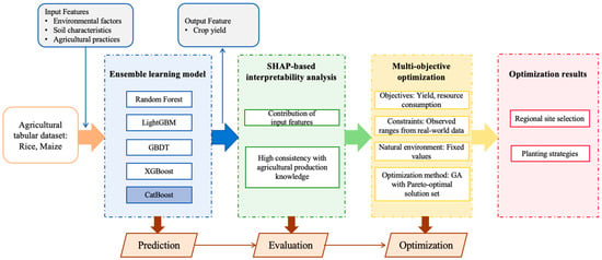
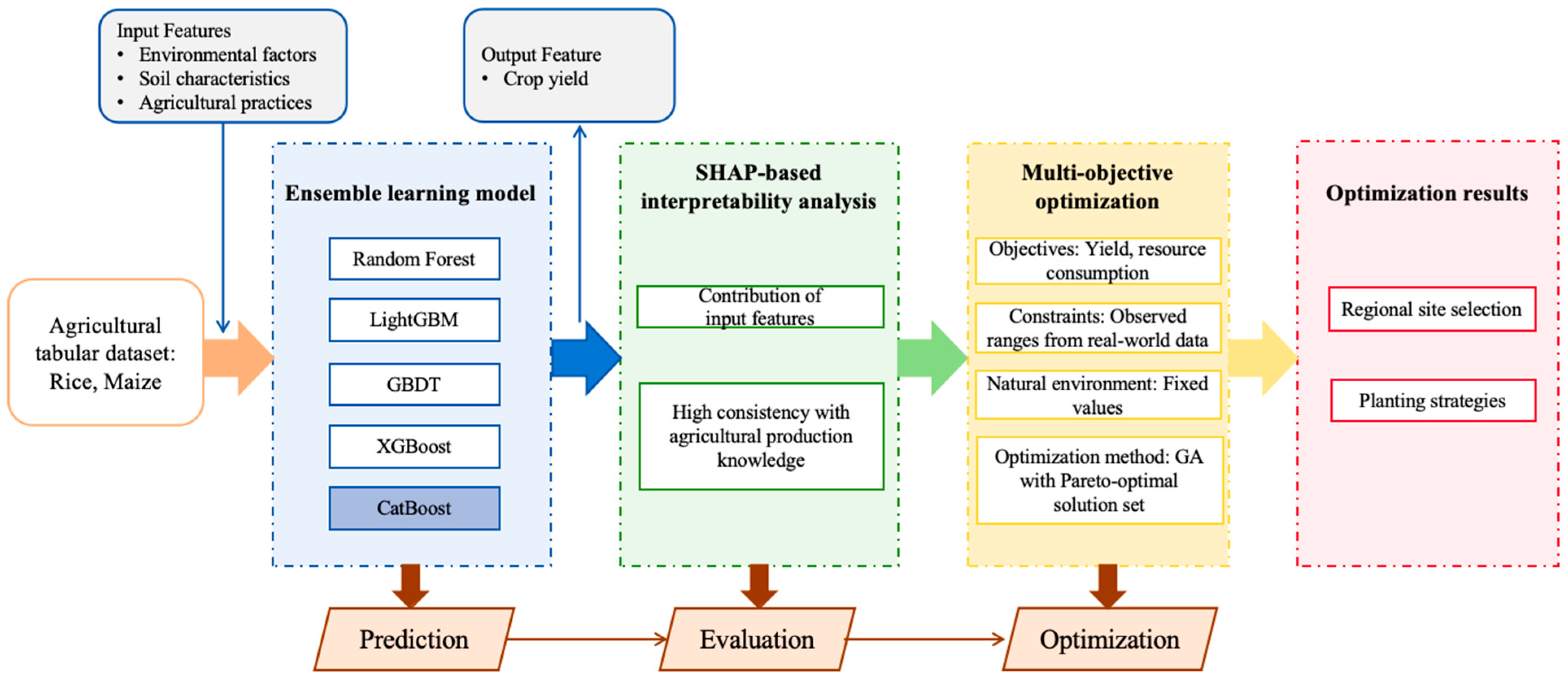
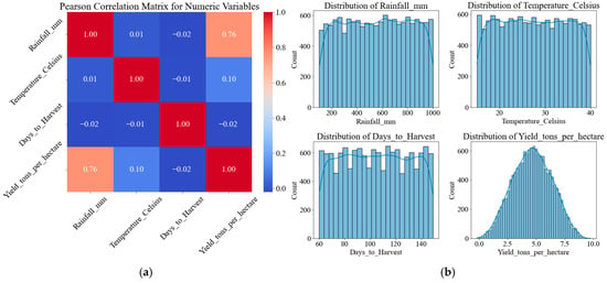
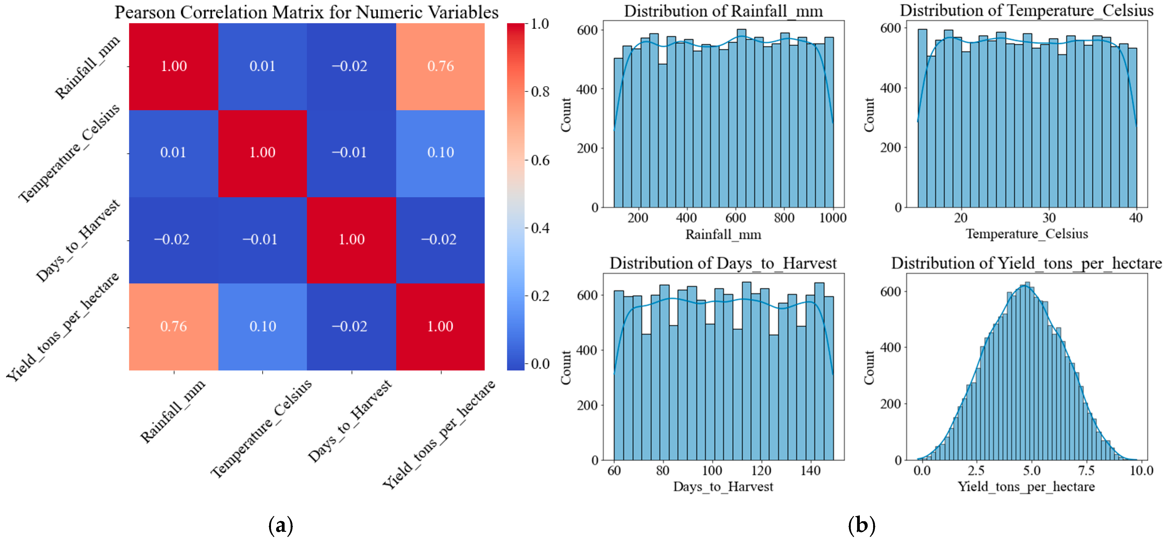
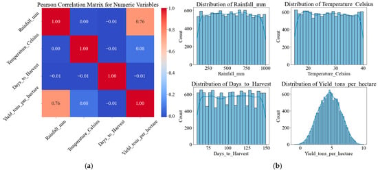
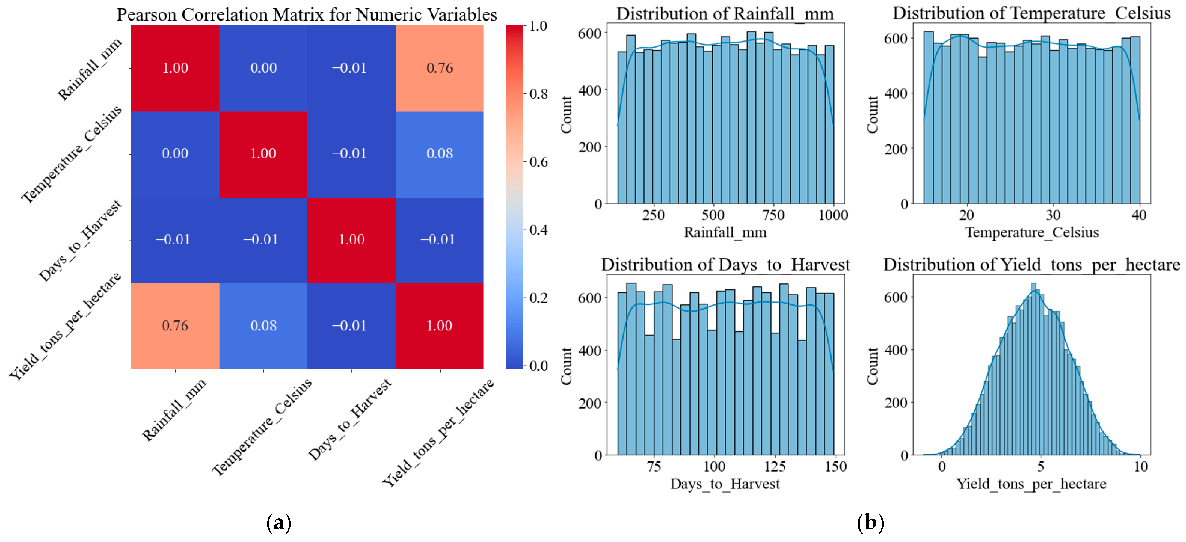
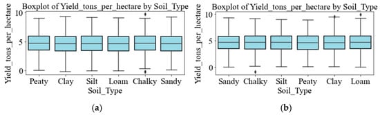
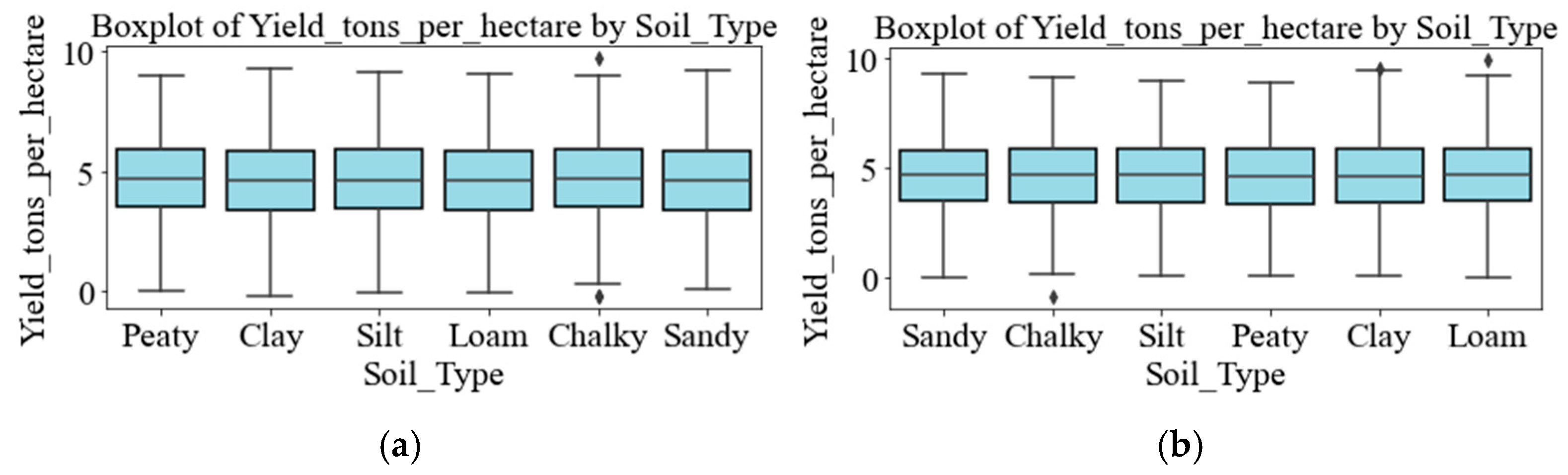
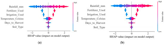
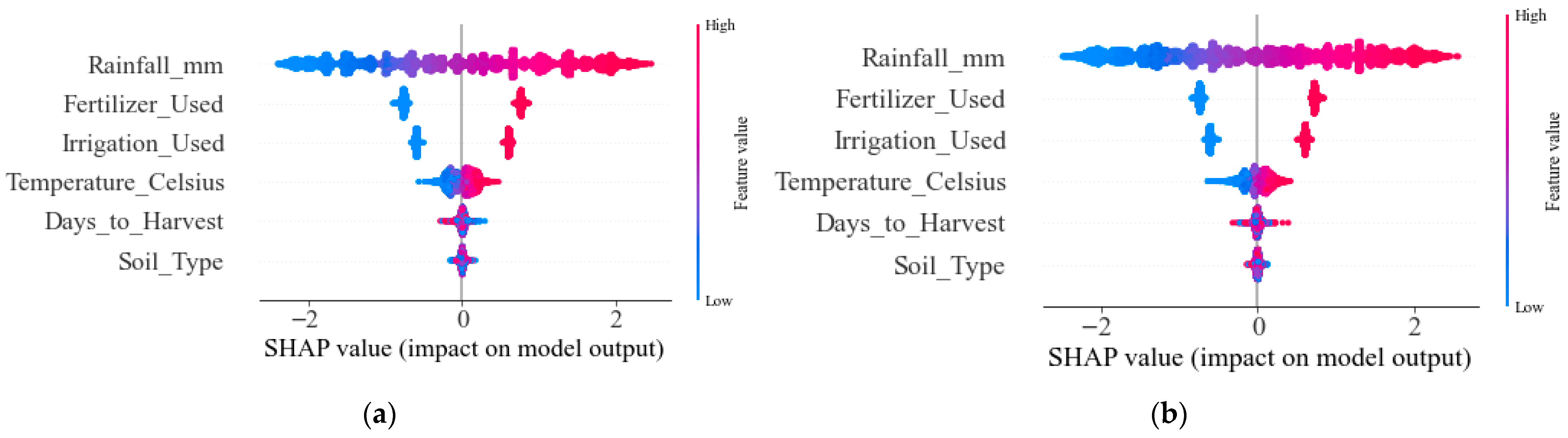
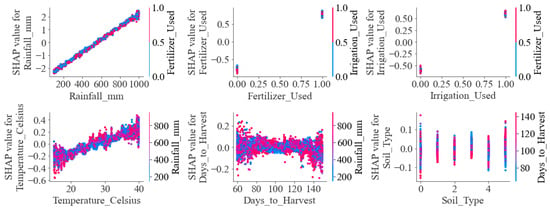
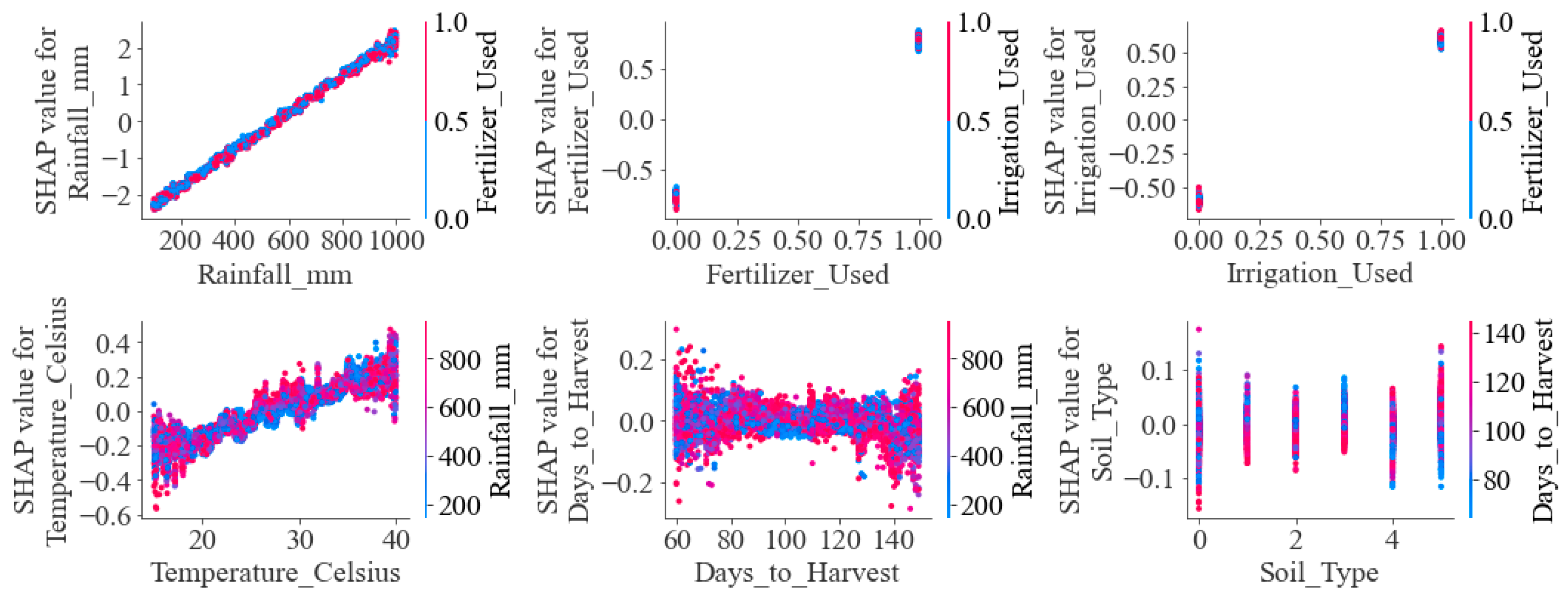
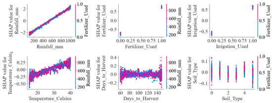
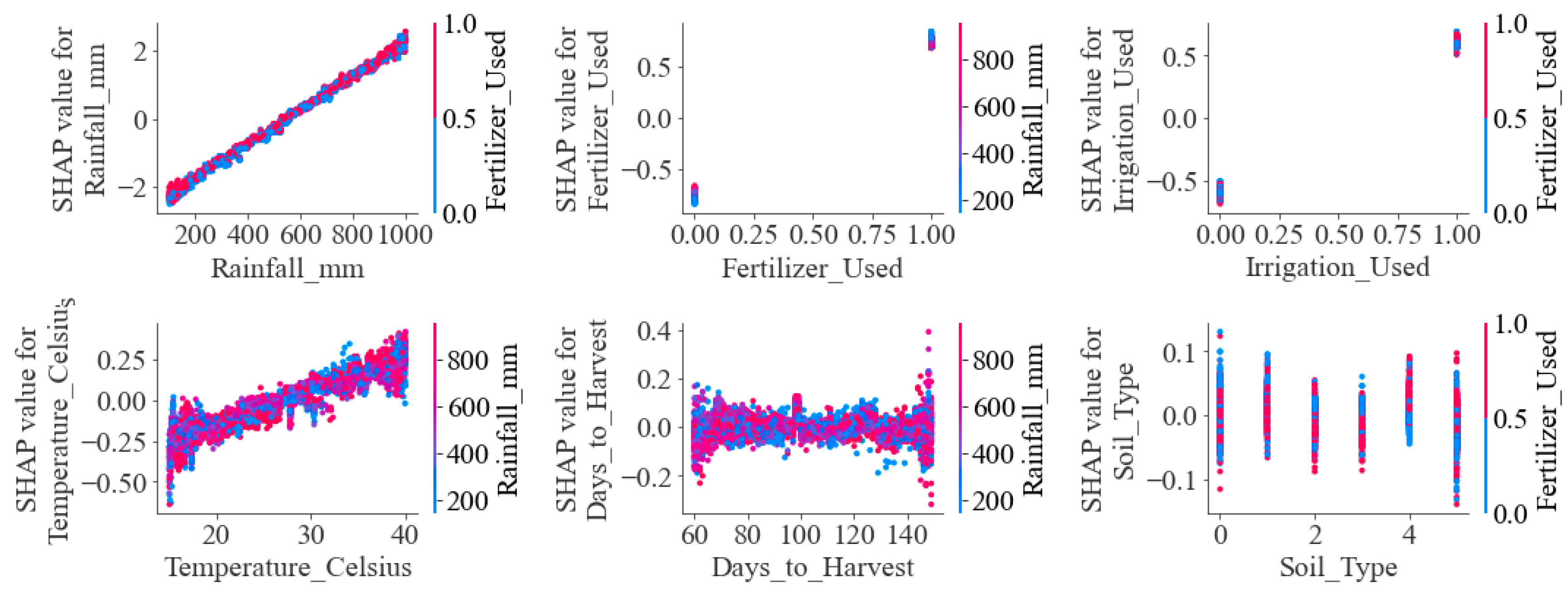
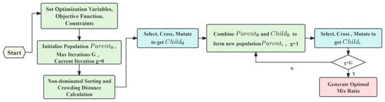
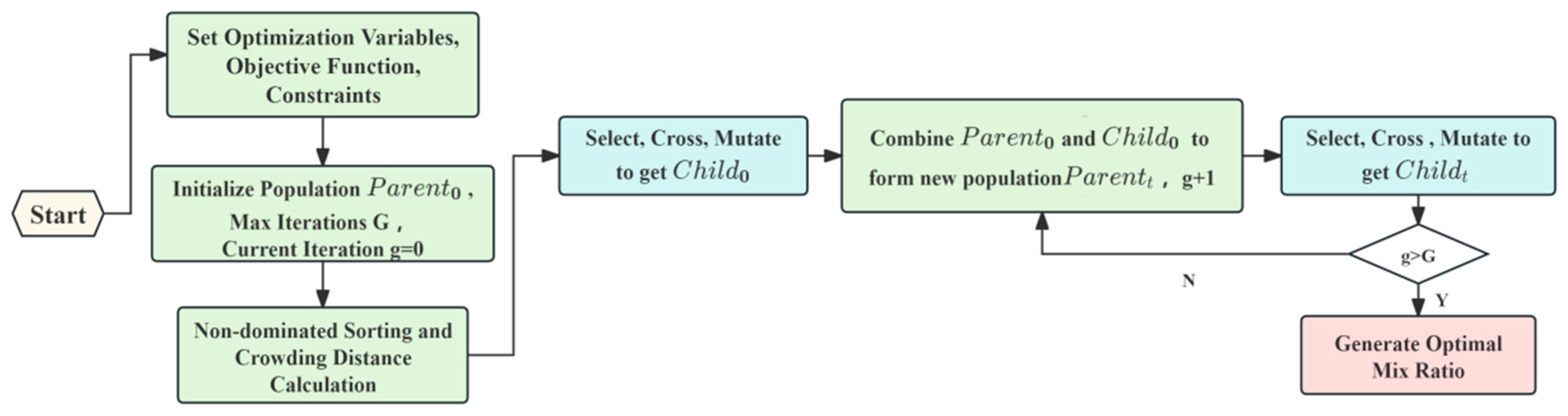
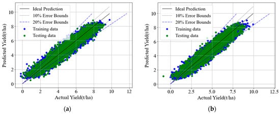
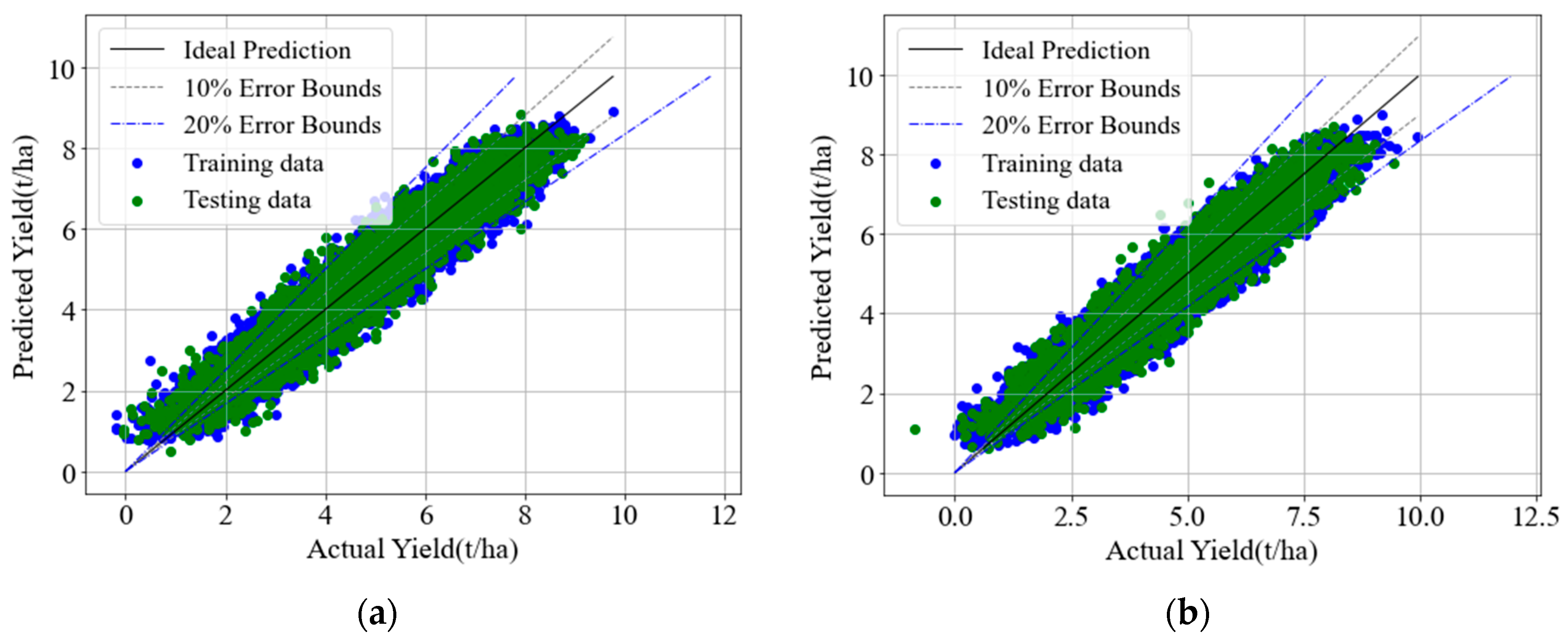
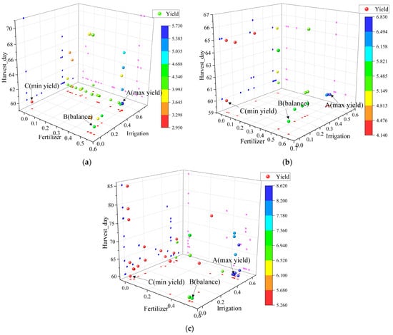
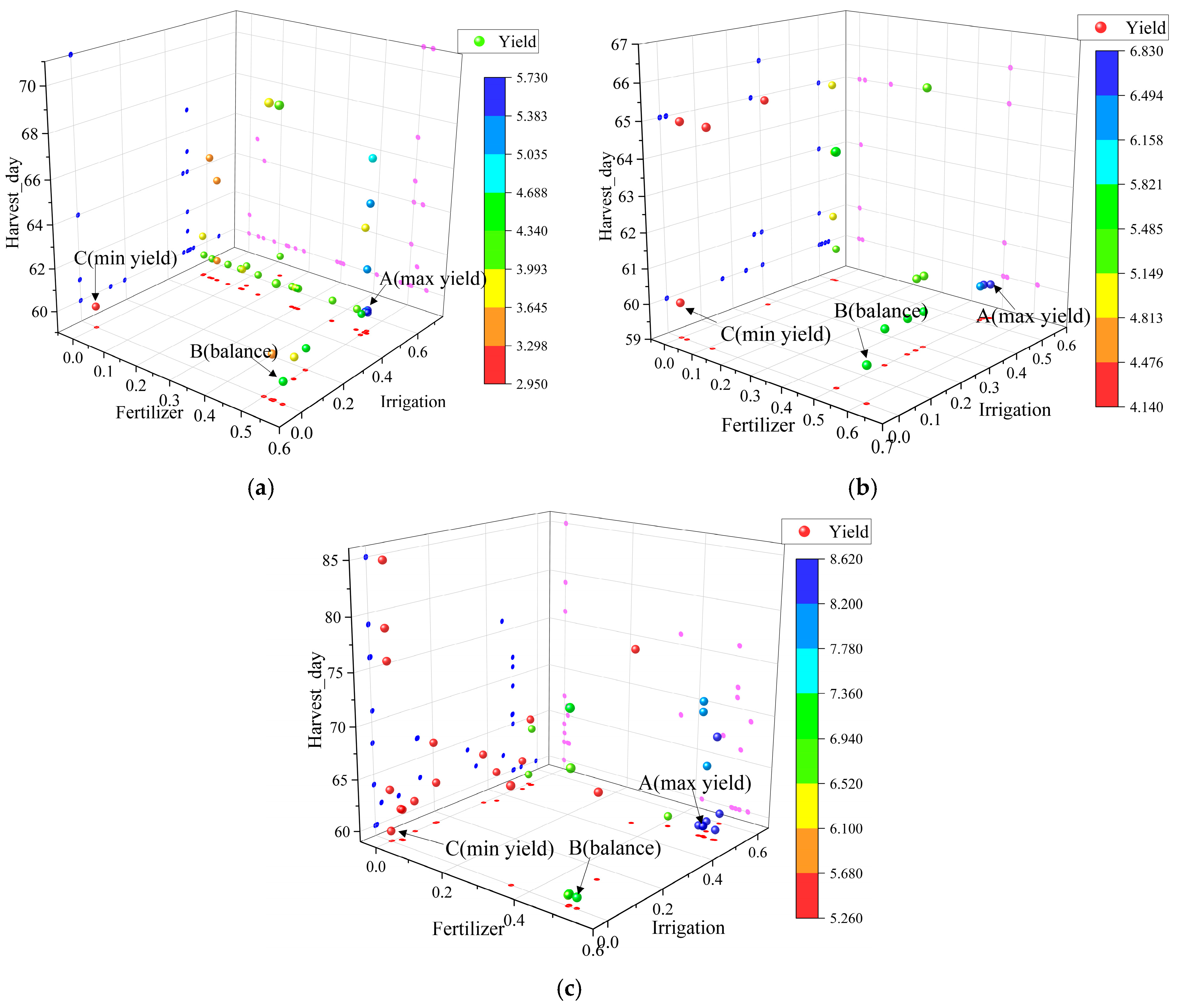
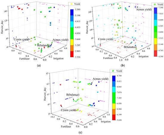
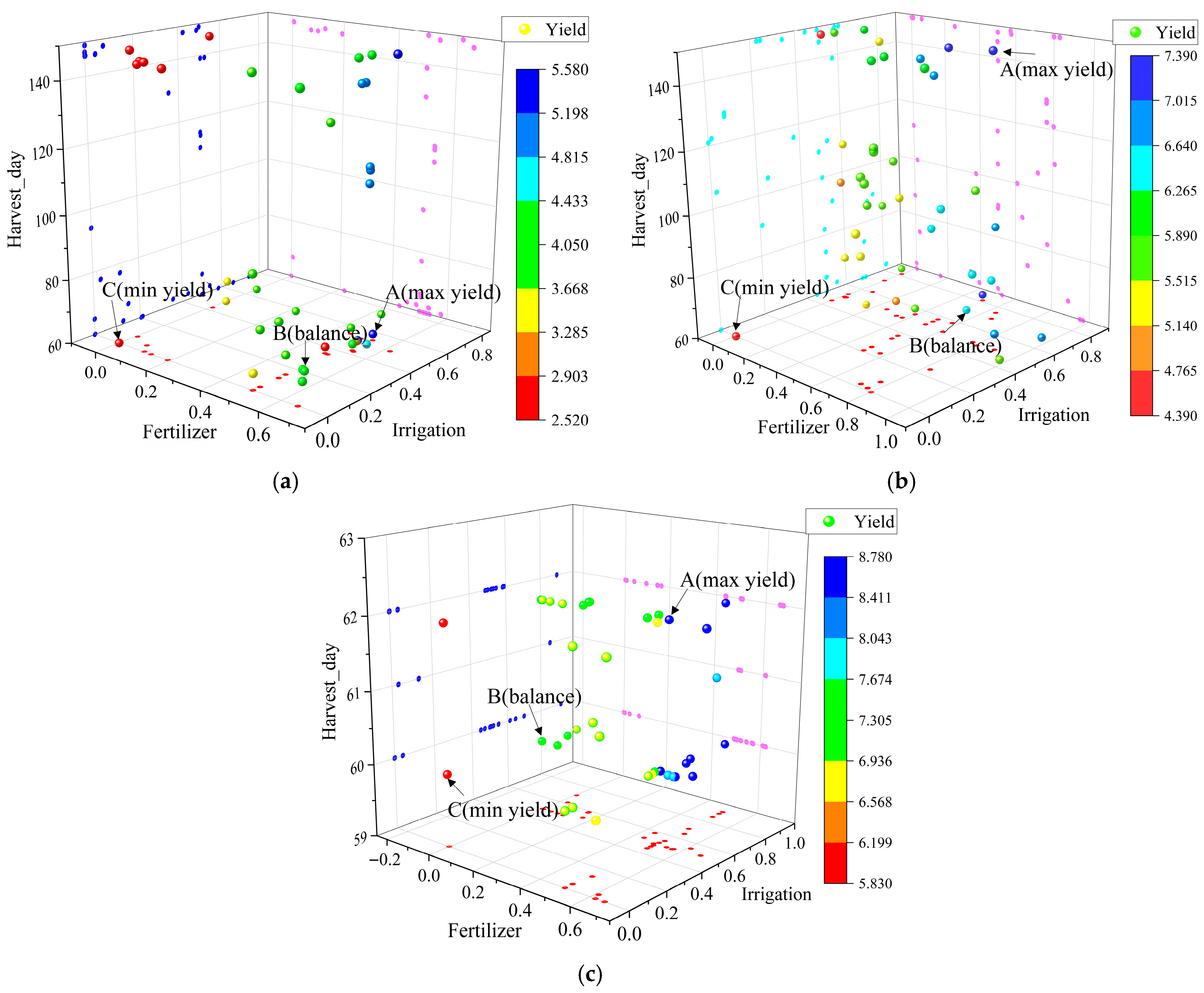

Disclaimer/Publisher’s Note: The statements, opinions and data contained in all publications are solely those of the individual author(s) and contributor(s) and not of MDPI and/or the editor(s). MDPI and/or the editor(s) disclaim responsibility for any injury to people or property resulting from any ideas, methods, instructions or products referred to in the content. |
© 2026 by the authors. Licensee MDPI, Basel, Switzerland. This article is an open access article distributed under the terms and conditions of the Creative Commons Attribution (CC BY) license.