Detection and Precision Application Path Planning for Cotton Spider Mite Based on UAV Multispectral Remote Sensing

Abstract

Cotton spider mites pose a significant threat to cotton production, while traditional manual investigation and blanket pesticide application are inefficient for precision pest management in large-scale cotton fields. To address this challenge, this study developed an integrated UAV multispectral remote sensing system for spider mite monitoring and precision spraying. Multispectral imagery was acquired from cotton fields in Shaya County, Xinjiang using UAV-mounted cameras, and vegetation indices including RDVI, MSAVI, SAVI, and OSAVI were selected through feature optimization. Comparative evaluation of three machine learning models (Logistic Regression, Random Forest, and Support Vector Machine) and two deep learning models (1D-CNN and MobileNetV2) was conducted. Considering classification performance and computational efficiency for real-time UAV deployment, Random Forest was identified as optimal, achieving 85.47% accuracy, an 85.24% F1-score, and an AUC of 0.912. The model generated centimeter-level spatial distribution maps for precise spray zone delineation. An improved NSGA-III multi-objective path optimization algorithm was proposed, incorporating PCA-based heuristic initialization, differential evolution operators, and co-evolutionary dual population strategies to optimize deadheading distance, energy consumption, operation time, turning frequency, and load balancing. Ablation study validated the effectiveness of each component, with the fully improved algorithm reducing IGD by 59.94% and increasing HV by 5.90% compared to standard NSGA-III. Field validation showed 98.5% coverage of infested areas with only 3.6% path repetition, effectively minimizing pesticide waste and phytotoxicity risks. This study established a complete technical pipeline from monitoring to application, providing a valuable reference for precision pest control in large-scale cotton production systems. The framework demonstrated robust performance across multiple field sites, though its generalization is currently limited to one geographic region and growth stage. Future work will extend its application to additional cotton varieties, growth stages, and geographic regions.

1. Introduction

Cotton, as a globally important economic crop and raw material for the textile industry, reached a global production of 25.4 million tons with a cultivation area exceeding 30 million hectares in the 2024–2025 season [1]. China is the world’s largest cotton producer and consumer, with Xinjiang cotton accounting for over 90% of national production, earning it the designation of “China’s Cotton Warehouse” [2]. Cotton spider mites are worldwide pests causing leaf chlorosis, yellowing, and even defoliation, severely affecting photosynthesis and boll development, with yield losses reaching 20–40% [3,4]. Traditional control methods primarily rely on uniform chemical pesticide application across entire fields, which not only leads to excessive pesticide use, environmental pollution, and natural enemy mortality, but also accelerates the development of mite resistance [5]. Therefore, achieving early precise monitoring and variable-rate pesticide application for mite infestations has become an urgent need for green cotton production.

Traditional pest monitoring mainly relies on manual field surveys, assessing pest occurrence through random sampling. Although this method can obtain relatively accurate local information, it has inherent deficiencies such as high labor intensity, time-consuming procedures, low spatial coverage, and strong subjectivity, making it difficult to meet the needs of large-scale mechanized cotton production in Xinjiang for timely, accurate, and comprehensive monitoring information. Remote sensing technology provides a new approach for large-area crop health monitoring by acquiring crop spectral information through non-contact methods [6]. However, although satellite remote sensing has broad coverage, it is limited by temporal resolution, spatial resolution, and cloud interference, making it difficult to meet the real-time precision monitoring needs at the field scale [7].

In recent years, Unmanned Aerial Vehicle (UAV) remote sensing has rapidly developed in the field of precision agriculture due to its advantages of high spatiotemporal resolution, low cost, and flexible mobility [8,9,10]. Pest and disease stress leads to decreased chlorophyll content in crop leaves, cell structure damage, and changes in water status, subsequently causing significant changes in spectral reflectance characteristics, thus providing a theoretical basis for UAV remote sensing monitoring of pests and diseases [11,12]. Currently, UAV multispectral remote sensing has made significant advances in pest detection. Wu et al. [13] and Yamada et al. [14] have achieved accurate identification of spider mite damage in jujube trees and cotton, respectively, through the fusion of spectral–spatial features and characteristic wavelength screening. Zhu et al. [15] have reviewed deep learning applications in UAV-based pest detection, showing that multispectral imaging combined with Convolutional Neural Networks achieves an 89–94% identification accuracy under favorable conditions. However, existing research mostly focuses on improving identification accuracy and optimizing bands, with limited exploration of how to effectively integrate detection results into precision application systems for operational implementation.

Achieving precision pesticide application based on the spatial distribution of pests and diseases requires support from intelligent application equipment and path planning technology. Plant protection UAVs have been rapidly promoted in China due to their advantages of high efficiency, flexibility, and uniform droplet deposition [16,17]. Intelligent path planning is the core technology for achieving precision application [18]. Recent advances have increasingly focused on integrating pest detection with variable-rate spraying systems. Li et al. [19] established a perception-decision-execution (PDE) framework systematically reviewing 168 publications on integrated UAV detection and adaptive variable-rate spraying technologies, demonstrating that PWM-based variable-rate spraying reduces pesticide usage by 30–50%. Complete workflows from identification to prescription-based application have been demonstrated, such as weed recognition coupled with UAV automatic variable-rate spraying achieving 30.1% pesticide reduction [20,21], and remote sensing-guided variable-rate application in disease control [22]. For multi-UAV coordination, Huang et al. [23] developed task allocation and path planning models for hilly terrains, swarm intelligence approaches have been applied to irregular farmland coverage [20,21] optimization [24], and collaborative systems achieved 46% energy reduction [25] and up to 40% path length reduction [26].

However, existing research has the following limitations: First, traditional full-coverage path planning methods (such as grid decomposition [27], boustrophedon paths [28], etc.) focus on complete coverage of the entire operational area without considering the spatial distribution heterogeneity of pests and diseases, leading to substantial ineffective spraying. Local obstacle avoidance planning methods (such as A* algorithm [29], RRT algorithm [30], etc.) can ensure safety but focus more on path feasibility rather than application efficiency. Second, although multi-objective optimization methods have been increasingly applied to agricultural path planning in recent years, such as optimizing flight parameters for droplet uniformity [31], real-time speed adjustment based on crop distribution [32], and deep reinforcement learning-based coverage planning [33], most studies optimize in regular areas with insufficient adaptability to irregular pest distribution patterns. Third, multi-UAV coordination research predominantly assumes predefined operational areas without integrating real-time pest distribution mapping into collaborative variable-rate application systems. Furthermore, research on small-sized pests like spider mites requiring centimeter-level detection and irregular infestation-based path planning remains limited. For multi-constraint multi-objective optimization problems, evolutionary algorithms have become the mainstream approach. The comparative study by Zhang et al. [34] showed that NSGA-III performs excellently in multi-objective path planning for agricultural robots; Li et al. [35] proposed an intelligent scheduling method based on NSGA-III and improved ant colony algorithm. However, existing research mostly compares algorithm performance in regular rectangular areas, with relatively limited systematic research on special needs in precision plant protection scenarios—such as irregular application areas caused by pest distribution and collaborative optimization of multiple performance indicators (deadheading distance, energy consumption, operation time, number of turns, load balancing).

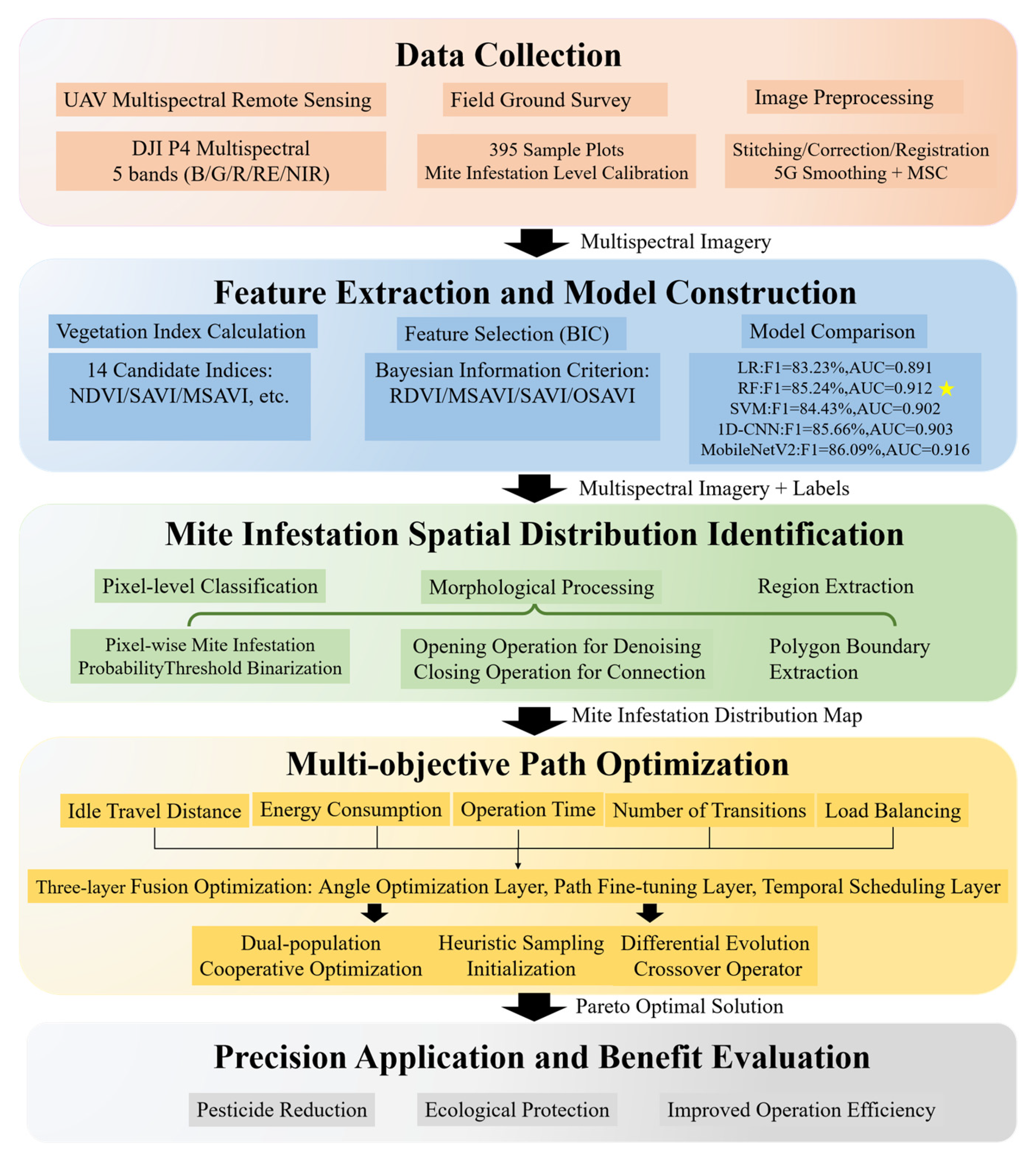
To address the above deficiencies, this study constructed a complete “remote sensing monitoring-intelligent identification-precision application” technical chain. UAV multispectral remote sensing was utilized to achieve intelligent identification of cotton field mite damage to precisely delineate pesticide application operational areas. For the path planning needs of irregular pest distribution areas, this study proposed an improved multi-objective path optimization algorithm that optimized operation paths through heuristic initialization, differential evolution, adaptive mutation, and multi-stage evolution strategies, thereby achieving precision variable-rate application and significantly reducing pesticide use while protecting the ecological environment. This research provides technical support for precision agriculture development and pesticide reduction with increased efficiency. The technical roadmap of this study is presented in Figure 1.

2. Materials and Methods

2.1. Spectral Data Acquisition

2.1.1. Experimental Site Selection and Background

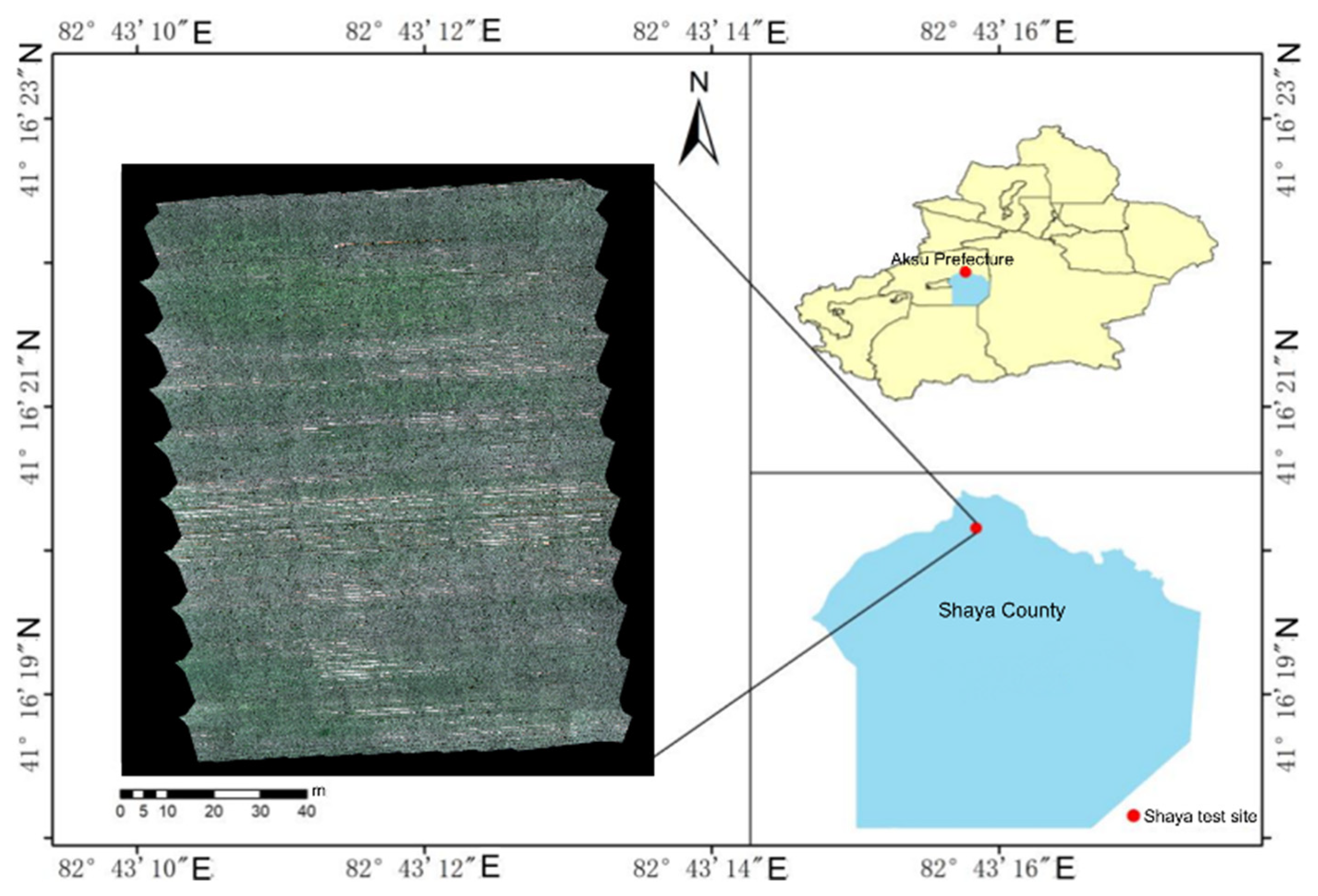
The experimental sites are located in Shaya County, Aksu Prefecture, Xinjiang Uygur Autonomous Region (41°16′21″ N–41°16′43″ N, 82°43′03″ E–82°43′31″ E). Four representative cotton fields with different plot locations, cotton varieties, and planting patterns were selected as experimental sites (Figure 2) to comprehensively test the model’s generalization ability. All experimental sites adopted drip irrigation under plastic film with integrated water and fertilizer technology, with complete irrigation facilities and standardized field management.

The investigation period was July–August 2025, when cotton was at the full bloom to early boll formation stages, which are the peak periods for spider mite occurrence. The main mite species in the fields were Tetranychus truncatus and Tetranychus turkestani. Mite damage showed obvious edge effects, mostly occurring from field edges, weed areas, and near shelter forests and spreading inward, exhibiting patchy or strip distribution characteristics. This study used the DJI Phantom Multispectral Real-Time Kinematic (RTK) quadcopter UAV platform to collect remote sensing data.

2.1.2. Data Collection Protocol

Flight missions were conducted from 28 July to 3 August 2025, between 12:00 and 14:00, coinciding with the peak occurrence period of spider mites during the flowering and boll stages of cotton. Environmental conditions during data collection were: temperature 28.5–35.2 °C, relative humidity 25–42%, wind speed 1.5–3.2 m/s, and sunshine duration >10 h daily, providing stable lighting conditions for multispectral imaging. Flight parameters were configured as follows: flight altitude of 20 m, ground sampling distance (GSD) of 1.1 cm, and both forward and side overlap rates of 70%. The flight path adopted an S-shaped pattern. Prior to each flight, radiometric calibration was performed using a 25% standard gray reflectance panel. By capturing images of the reference panel with known reflectance, a conversion relationship between Digital Number (DN) values and surface reflectance was established, providing a baseline for subsequent radiometric correction. Concurrent with aerial data acquisition, ground-truth surveys were conducted to establish training labels.

Ground-truth data were collected concurrently with UAV flights using a stratified S-shaped sampling approach. A total of 395 georeferenced sampling points were established across the four sites, with coordinates recorded using a high-precision RTK-GPS device (±2–5 cm accuracy) to enable geometric correction.

At each sampling point, spider mite damage severity was assessed following the Chinese National Standard GB/T 15802-2011. Ten cotton plants were randomly selected within a 1 m² quadrat, with three leaves examined per plant (one each from upper, middle, and lower canopy). Each leaf was classified into four damage grades: Grade 0 (healthy, no symptoms), Grade 1 (scattered yellow spots), Grade 2 (reddish-brown discoloration on <1/3 of leaf area), and Grade 3 (discoloration on ≥1/3 of leaf area). Spider mite feeding produced distinctive symptoms including chlorotic stippling, leaf bronzing, fine webbing on undersides, and premature senescence.

For binary classification modeling, the average damage grade across 30 examined leaves (10 plants × 3 leaves per plant) was calculated for each sampling point. Following regional IPM guidelines, points with average grade ≥2.0 were classified as “mite-infested” (requiring intervention), while those with grade <2.0 were classified as “healthy” (below economic threshold). Representative spider mite infestation data from the survey are presented in

Table 1. Partial mite survey data.

No.	Latitude (°N)	Longitude (°E)	Mite Infestation
1	41.27193222	82.72034569	0 (Healthy)
2	41.27191855	82.72032373	0 (Healthy)
3	41.27197146	82.72037654	0 (Healthy)
4	41.27206712	82.72029264	0 (Healthy)
5	41.27207192	82.72033700	0 (Healthy)
6	41.2721709	82.72025131	0 (Healthy)
……	……	……	……
394	41.27250806	82.72015163	1 (Infested)
395	41.27249433	82.72008869	1 (Infested)

Note: No., Sequential identification number of georeferenced ground survey sampling points. Mite infestation classified based on field survey following standardized protocols.

.

2.2. Multispectral Image Preprocessing

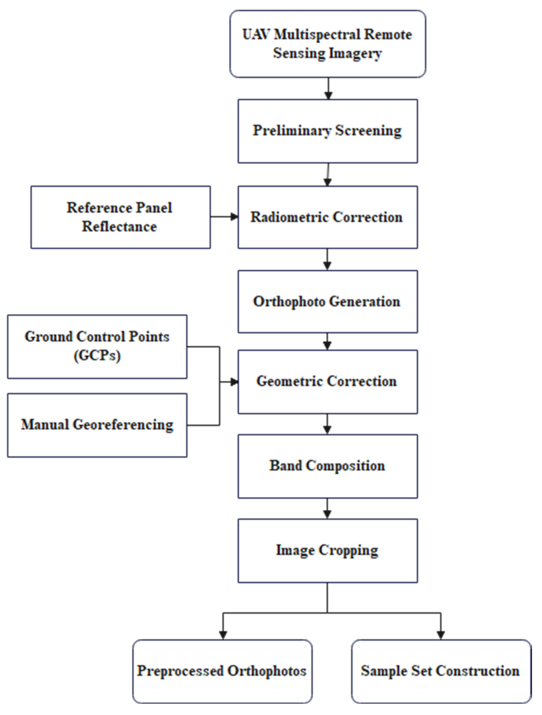
Multispectral image preprocessing was a critical step to ensure mite identification accuracy, including image stitching, geometric correction, radiometric correction, and spectral data processing steps, as shown in Figure 3. First, preliminary screening of raw images was conducted to remove abnormally exposed images, followed by automatic stitching using DJI Terra software (V4.4.0) and radiometric correction using 25% standard gray panel images collected before flights. Based on 7 ground control points, geometric correction of orthophotos was performed using ENVI 5.3, five-band images were synthesized, and edge distortion areas were cropped. Based on the coordinates of 395 ground survey sample points, corresponding regions of interest (ROI) were extracted from the crop classification images, and the mean spectral reflectance of pixels within each ROI was calculated as the spectral characteristics of the cotton canopy in that area, obtaining a total of 1560 valid sample data points (780 healthy, 780 mite-damaged).

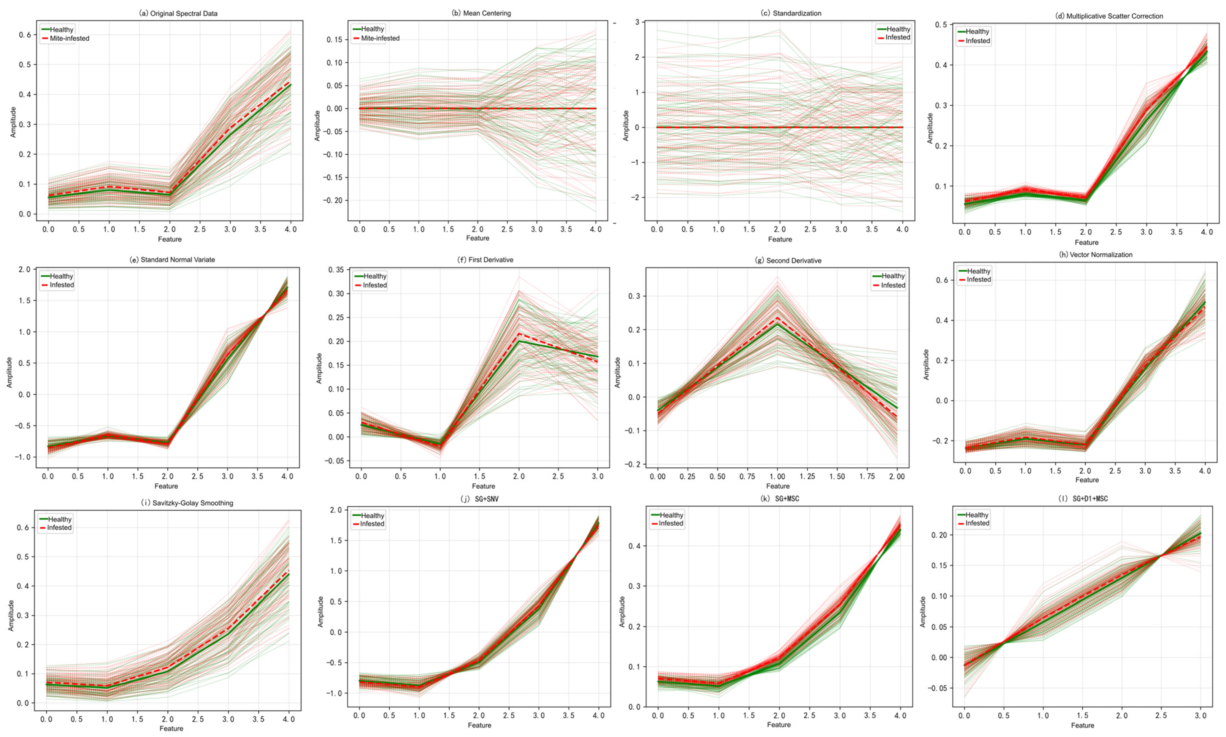
This study systematically evaluated 12 spectral preprocessing approaches, including 8 individual methods (Mean Centering MC, Standardization STD, Multiplicative Scatter Correction MSC, Standard Normal Variate transformation SNV, First Derivative D1, Second Derivative D2, Vector Normalization VN, and Savitzky–Golay smoothing SG) and 3 combinations (SG+SNV, SG+MSC, SG+D1+MSC). Visualization methods were used to analyze the spectral separation between healthy and mite-damaged samples under different preprocessing methods. Results are presented in Figure 4.

As shown in the figure, green solid lines represent the reflectance of healthy samples across 5 bands, while red dashed lines represent the reflectance of mite-damaged samples across 5 bands. In the original spectral data, there was considerable overlap between healthy and damaged samples, making discrimination difficult. After preprocessing, Figure 4d shows that Multiplicative Scatter Correction provided good discrimination in the near-infrared band, and Figure 4i shows that SG smoothing filtering improved discrimination. Among all spectral data processing methods, Figure 4k demonstrates that the combination of SG smoothing filtering and Multiplicative Scatter Correction achieved the best discrimination in the near-infrared band. In conclusion, this study selected the combination of SG smoothing filtering and Multiplicative Scatter Correction to process spectral data for subsequent experiments.

2.2.1. Data Augmentation

The original 1560 samples were first randomly divided into training set (1092 samples), validation set (312 samples), and test set (156 samples) at a ratio of 7:2:1. Data augmentation was then performed only on the training set, while validation and test sets remained unaugmented to ensure unbiased evaluation. Considering the characteristics of multispectral ROI data and actual field conditions, the following augmentation strategies were adopted:

(1)

Gaussian noise addition: Gaussian noise with mean 0 and standard deviation 0.02 was added to spectral reflectance values of each band to simulate sensor noise and environmental interference;

(2)

Spectral random perturbation: Random perturbations within ±5% range were applied to reflectance values of each band to simulate spectral response variations under different moments and lighting conditions;

(3)

SMOTE over-sampling: Synthetic Minority Over-sampling Technique (SMOTE) was used to synthesize and expand samples, ensuring class balance. It should be noted that SMOTE-generated samples were used exclusively for training, while all validation and test evaluations were conducted on original unaugmented data to ensure that model performance metrics reflect real-world detection capability rather than synthetic pattern recognition.

Through the above augmentation strategies, the training set was expanded from 1092 to 3267 samples (approximately 3-fold increase), while the validation set (312 samples) and test set (156 samples) remained unchanged to ensure unbiased model evaluation.

2.3. Vegetation Index Calculation

After preprocessing, to enhance the discriminability of mite damage features, feature expansion through vegetation indices was necessary. Vegetation indices can enhance vegetation information, suppress background interference, and amplify stress signals through mathematical combinations of different band reflectances. Combining the band configuration of the UAV multispectral sensor and experience in remote sensing monitoring of crop pests and diseases, 14 vegetation indices were selected as candidate features, including normalized indices (NDVI, GNDVI, etc.), soil-adjusted indices (RDVI, MSAVI, SAVI, OSAVI, etc.), and other types of indices.

To identify vegetation indices most sensitive to mite damage, the mean Vegetation Index of all pixels within each ROI was calculated as the sample feature value, and Pearson correlation analysis was performed (

Table 2. Correlation between spectral indices and mite occurrence.

No.	Spectral Index	Correlation Coefficient (R)	|R|	Rank
1	B1	−0.034188	0.034188	19
2	B2	−0.051205	0.051205	18
3	B3	0.079912 *	0.079912	17
4	B4	−0.268461 **	0.268461	16
5	B5	−0.427808 **	0.427808	8
6	NDVI	−0.369989 **	0.369989	9
7	GNDVI	−0.323088 **	0.323088	15
8	NDGI	−0.343998 **	0.343998	14
9	RDVI	−0.503456 **	0.503456	1
10	RVI	−0.36789 **	0.36789	11
11	DVI	−0.479937 **	0.479937	5
12	TVI	−0.479635 **	0.479635	6
13	LCI	−0.34549 **	0.34549	13
14	EVI	−0.461857 **	0.461857	7
15	MSR	−0.369752 **	0.369752	10
16	SAVI	−0.501463 **	0.501463	3
17	MSAVI	−0.502783 **	0.502783	2
18	OSAVI	−0.48342 **	0.48342	4
19	VARI	−0.358366 **	0.358366	12

Note: No., Feature index; B1–B5, Multispectral bands; RDVI, Renormalized Difference Vegetation Index; MSAVI, Modified Soil-Adjusted Vegetation Index; SAVI, Soil-Adjusted Vegetation Index; OSAVI, Optimized Soil-Adjusted Vegetation Index; GNDVI, Green Normalized Difference Vegetation Index; NDVI, Normalized Difference Vegetation Index; NDGI, Normalized Difference Greenness Index; RVI, Ratio Vegetation Index; DVI, Difference Vegetation Index; TVI, Transformed Vegetation Index; LCI, Leaf Chlorophyll Index; EVI, Enhanced Vegetation Index; MSR, Modified Simple Ratio; VARI, Visible Atmospherically Resistant Index. |R|, Absolute value of correlation coefficient; Rank, Ranking by absolute correlation strength. * p < 0.05; ** p < 0.01.

). Results showed that except for blue and green bands, all other spectral features showed significant or highly significant negative correlations with mite occurrence (p < 0.05 or p < 0.01). Soil-adjusted indices (RDVI, MSAVI, SAVI, OSAVI) had the largest absolute correlation coefficients with mite damage (|R| > 0.48), significantly higher than traditional Normalized Difference Vegetation Index (NDVI, |R| = 0.37). This is because, when cotton canopy coverage is incomplete, soil background has a significant impact on spectral reflectance, and soil-adjusted indices can suppress soil background interference by introducing adjustment factors, more truly reflecting the degree of mite stress. Therefore, RDVI, MSAVI, SAVI, and OSAVI were identified as the most promising features for mite identification modeling, subject to further optimization in subsequent analysis.

2.4. Mite Damage Identification Model Construction and Validation

To identify the optimal classification method for cotton spider mite detection, 3 traditional machine learning algorithms were systematically evaluated: Logistic Regression (LR), Random Forest (RF), and Support Vector Machine (SVM). Additionally, two representative deep learning architectures—1D Convolutional Neural Network (1D-CNN) and MobileNetV2—were implemented as comparative baselines to assess whether automatic feature learning could outperform domain-knowledge-driven feature engineering in this application. 1D-CNN was selected as the simplest convolutional architecture capable of learning higher-order nonlinear combinations from input features, with demonstrated effectiveness in spectral data processing and crop stress detection [36]. MobileNetV2 represented state-of-the-art lightweight architectures specifically designed for resource-constrained edge deployment, making it particularly suitable for UAV-based real-time applications [37,38]. Both models can achieve reasonable performance on small-to-medium datasets, unlike transformer-based architectures which require substantially larger training sets. Larger CNN variants (e.g., ResNet, EfficientNet) were excluded as they are designed for high-dimensional inputs and would be severely over-parameterized for 4-dimensional feature vectors [39]. These two models represent different levels of architectural complexity—1D-CNN as a minimal baseline for spectral feature learning, and MobileNetV2 as a representative lightweight architecture—providing a comprehensive comparison for selecting optimal models for UAV-based pest monitoring systems. All models were trained using the same four optimized vegetation indices (RDVI, MSAVI, SAVI, OSAVI) as input features to ensure fair comparison.

2.4.1. Logistic Regression Model

Logistic Regression (LR) is a classic binary classification machine learning algorithm widely applied in remote sensing classification and medical diagnosis. Compared to complex nonlinear classifiers, LR has advantages such as simple model structure, easy-to-interpret parameters, high training efficiency, and relatively lower risk of overfitting on small sample data when properly regularized, making it particularly suitable for application scenarios in this study where sample size is limited and clear feature contributions are needed. The core idea of LR is to map the output of a linear regression model to the (0,1) interval through logit transformation as the probability estimate of a sample belonging to a certain category. For the binary classification problem of mite identification, the Logistic Regression model can be expressed as

$$P(Y=1|x_1,x_2,\cdots ,x_k)={\displaystyle \frac{\mathit{exp}({\beta }_0+{\beta }_1{x}_1+{\beta }_2{x}_2+\cdots +{\beta }_k{x}_k)}{1+\mathit{exp}({\beta }_0+{\beta }_1{x}_1+{\beta }_2{x}_2+\cdots +{\beta }_k{x}_k)}}$$

(1)

$$Y=ln\left({\displaystyle \frac{P}{1-P}}\right)={\beta }_0+{\beta }_1{x}_1+{\beta }_2{x}_2+\cdots +{\beta }_k{x}_k$$

(2)

where P is the predicted probability of mite infestation (0 ≤ P ≤ 1), Y is the log-odds (logit), x₁, x₂, …, $x_k$ are the k input features (in this study, k = 4: RDVI, MSAVI, SAVI, OSAVI), β₀ is the intercept, and β₁, β₂, …, ${\beta }_k$ are the regression coefficients.

2.4.2. Random Forest

Random Forest (RF) is an ensemble learning method based on decision tree bagging that has been successfully applied in remote sensing classification and agricultural pest detection. Compared to traditional linear classifiers, RF offers several advantages: (1) the ability to capture nonlinear relationships between vegetation indices and pest damage without manual feature engineering; (2) robustness to outliers and noise through ensemble averaging of multiple decision trees; (3) reduced overfitting risk through random feature selection and bootstrap sampling; (4) built-in feature importance evaluation for model interpretability. The RF classifier constructs multiple decision trees during training and outputs the mode of classes for classification tasks, formulated as

$$\widehat{y}=model[h_1\left(x\right),h_2\left(x\right),\dots ,h_b\left(x\right)]$$

(3)

where $h_b\left(x\right)$ represents the prediction of the b-th decision tree (b = 1, 2, …, B), B is the total number of trees, and ŷ is the final prediction obtained by majority voting.

2.4.3. Support Vector Machine

Support Vector Machine seeks to find an optimal hyperplane that maximizes the margin between different classes in feature space. For non-linearly separable problems, SVM employs kernel functions to map data into higher-dimensional space. The Radial Basis Function (RBF) kernel was adopted in this study, defined as

$$K\left(x_i,x_j\right)=\exp \left(-\gamma {‖x_i-x_j‖}^2\right)$$

(4)

where $‖x_i-x_j‖$ denotes the Euclidean distance between the two samples, and $\gamma$ is the kernel coefficient controlling the influence range of a single training sample.

2.4.4. Deep Learning Baselines

To provide comprehensive performance evaluation, two representative deep learning architectures were implemented as comparative baselines: 1D Convolutional Neural Network (1D-CNN) and MobileNetV2.

The 1D-CNN employed 3 convolutional blocks with progressively increasing filter sizes (32, 64, 128), followed by global average pooling and fully connected layers for binary classification. MobileNetV2 was adapted for 1D spectral input using depthwise separable convolutions to maintain computational efficiency. Both models were trained using Adam optimizer with early stopping to prevent overfitting, following the same data split and augmentation strategies as traditional machine learning models.

2.4.5. Model Training and Hyperparameter Optimization

As described in Section 2.2.1, the original 1560 samples were divided into training set (1092 samples), validation set (312 samples), and test set (156 samples) at a ratio of 7:2:1. After data augmentation, the training set was expanded to 3267 samples, while the validation and test sets remained unchanged to ensure unbiased model evaluation.

To determine the optimal feature combination, a forward stepwise regression strategy was adopted using Logistic Regression as the selection framework, according to the correlation ranking results from Section 2.3, adding vegetation indices to the model sequentially. After adding each variable, the Bayesian Information Criterion (BIC) value was calculated. BIC comprehensively considers model goodness of fit and complexity, with smaller values indicating better model performance. The feature selection results for different numbers of independent variables are shown in

Table 3. BIC values of different Logistic Regression equations.

n	Logistic Regression Equation	BIC Value
1	2.538 − 4.917 × RDVI	13.860
2	4.742 − 3.765 × RDVI − 5.011 × MSAVI	13.826
3	6.073 − 3.292 × RDVI − 4.383 × MSAVI − 3.519 × SAVI	13.843
4	7.009 − 3.089 × RDVI − 4.111 × MSAVI − 3.304 × SAVI − 2.374 × OSAVI	13.810
5	7.414 − 2.771 × RDVI − 3.698 × MSAVI − 2.964 × SAVI − 2.179 × OSAVI − 2.978 × DVI	13.860
6	11.884 − 0.465 × RDVI − 0.704 × MSAVI − 0.506 × SAVI − 0.737 × OSAVI − 0.022 × DVI − 0.464 × TVI	14.072
…	……	…
19	——	14.188

Note: BIC, Bayesian Information Criterion (lower values indicate better model performance); n, number of input features.

, where n is the number of input feature variables.

Results showed that as the number of features increased from 1 to 4, BIC values gradually decreased, reaching the minimum value of 13.810 when including the four features RDVI, MSAVI, SAVI, and OSAVI; BIC values increased after adding more features. When 19 independent variables were introduced, the BIC value reached its highest, indicating that although the addition of extra features slightly improved goodness of fit, the increased model complexity exceeded the magnitude of fitting improvement, leading to increased BIC values. Therefore, RDVI, MSAVI, SAVI, and OSAVI were determined as the optimal feature combination. To ensure fair comparison across different classification algorithms, these four features were uniformly applied to all three models (LR, RF, and SVM) for subsequent training and evaluation, allowing the performance comparison to reflect the inherent capabilities of different algorithms rather than differences in feature sets.

Using these four optimal features, systematic hyperparameter optimization was performed for each model using grid search combined with 5-fold cross-validation, with F1-score as the optimization objective. The parameter search spaces were configured as follows:

For Logistic Regression: regularization strength C ∈ [0.01, 0.1, 1, 10, 100], regularization type penalty ∈ [‘l1’, ‘l2’], ${class}_{\mathrm{w}\mathrm{e}\mathrm{i}\mathrm{g}\mathrm{h}\mathrm{t}}$ ∈ [None, ‘balanced’], and solver ∈ [‘liblinear’, ‘saga’], ${max}_{\mathrm{i}\mathrm{t}\mathrm{e}\mathrm{r}}$ ∈ [500, 1000, 2000]. Optimization results showed that the optimal parameters were C = 100, penalty = ‘l1’, solver = ‘liblinear’, ${max}_{\mathrm{i}\mathrm{t}\mathrm{e}\mathrm{r}}$ = 1000.

For Random Forest: number of trees $n_{\mathrm{e}\mathrm{s}\mathrm{t}\mathrm{i}\mathrm{m}\mathrm{a}\mathrm{t}\mathrm{o}\mathrm{r}\mathrm{s}}$ ∈ [100, 200, 300, 500], maximum tree depth ${max}_{\mathrm{d}\mathrm{e}\mathrm{p}\mathrm{t}\mathrm{h}}$ ∈ [10, 20, 30, None], minimum samples for split ${min}_{{\mathrm{s}\mathrm{a}\mathrm{m}\mathrm{p}\mathrm{l}\mathrm{e}\mathrm{s}}_{split}}$ ∈ [2, 5, 10], minimum samples per leaf ${min}_{{\mathrm{s}\mathrm{a}\mathrm{m}\mathrm{p}\mathrm{l}\mathrm{e}\mathrm{s}}_{leaf}}$ ∈ [1, 2, 4], and maximum features ${max}_{\mathrm{f}\mathrm{e}\mathrm{a}\mathrm{t}\mathrm{u}\mathrm{r}\mathrm{e}}$ ∈ [‘sqrt’, ‘log2’]. The optimal parameters were determined as: $n_{\mathrm{e}\mathrm{s}\mathrm{t}\mathrm{i}\mathrm{m}\mathrm{a}\mathrm{t}\mathrm{o}\mathrm{r}\mathrm{s}}$ = 300, ${max}_{\mathrm{d}\mathrm{e}\mathrm{p}\mathrm{t}\mathrm{h}}$ = 20, ${min}_{{\mathrm{s}\mathrm{a}\mathrm{m}\mathrm{p}\mathrm{l}\mathrm{e}\mathrm{s}}_{split}}$ = 5, ${min}_{{\mathrm{s}\mathrm{a}\mathrm{m}\mathrm{p}\mathrm{l}\mathrm{e}\mathrm{s}}_{leaf}}$ = 2, ${max}_{\mathrm{f}\mathrm{e}\mathrm{a}\mathrm{t}\mathrm{u}\mathrm{r}\mathrm{e}}$ = ‘sqrt’.

For SVM: regularization parameter C ∈ [0.1, 1, 10, 100, 1000], kernel type ∈ [‘rbf’, ‘linear’, ‘poly’], RBF kernel coefficient $\gamma$∈ [0.001, 0.01, 0.1, 1, ‘scale’], and ${class}_{\mathrm{w}\mathrm{e}\mathrm{i}\mathrm{g}\mathrm{h}\mathrm{t}}$ ∈ [None, ‘balanced’]. The optimal parameters were: C = 100, $\gamma$ = ‘scale’, kernel=‘rbf’.

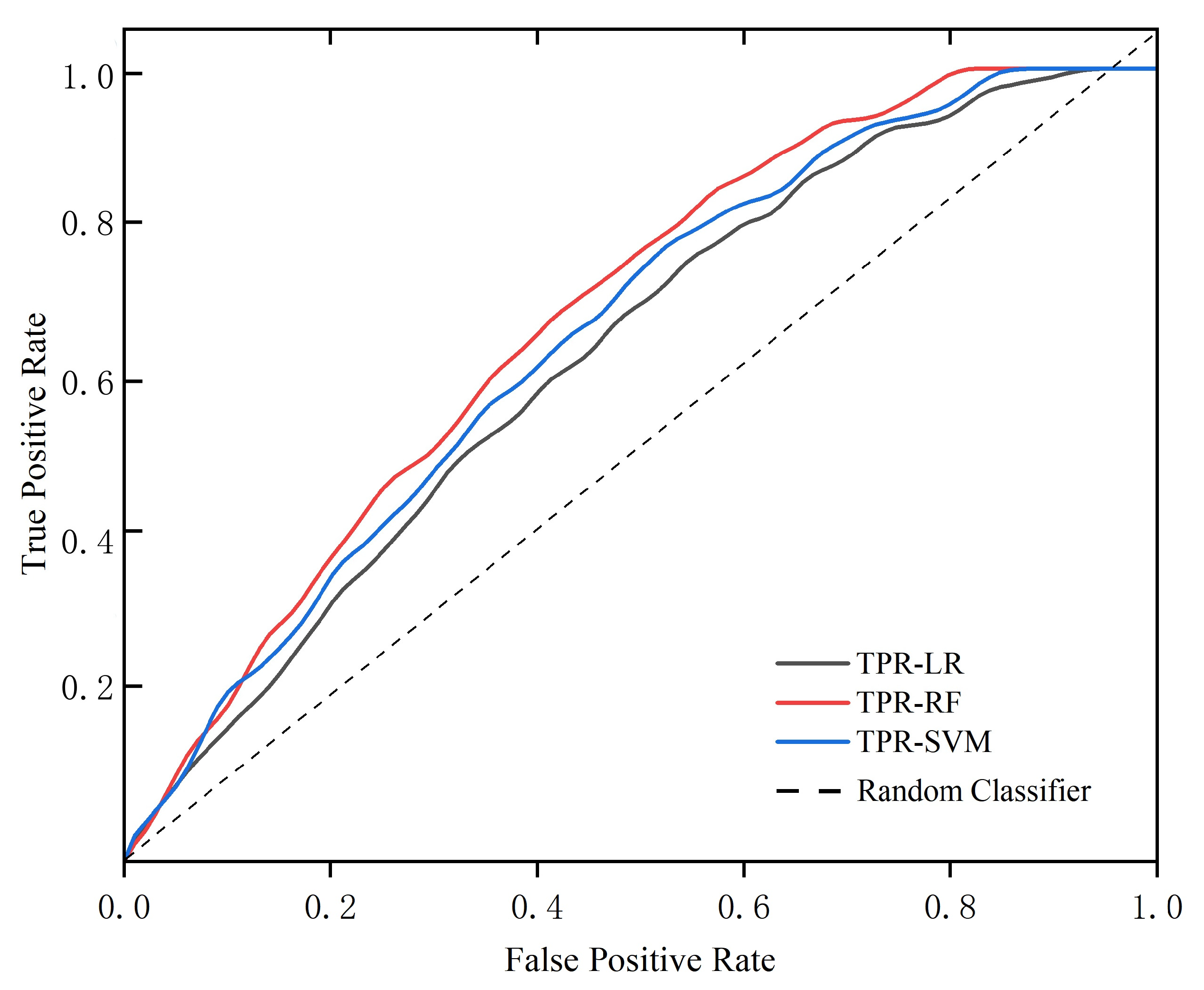
After hyperparameter optimization using cross-validation on the training set, the three models with optimal parameters were trained on the full training set and then evaluated on the independent validation set. Multiple metrics were assessed, including accuracy, precision, recall, F1-score, and area under the Receiver Operating Characteristic (ROC) curve (AUC). The detailed performance comparison is presented in

Table 4. Comparison of model evaluation results.

Model	Accuracy	Precision	Recall	F1-Score	AUC	Inference Time (ms)
LR	83.28%	84.52%	81.97%	83.23%	0.891	2.1
RF	85.47%	86.31%	84.19%	85.24%	0.912	8.5
SVM	84.62%	85.78%	83.12%	84.43%	0.902	5.3
1D-CNN	84.91%	86.11%	85.21%	85.66%	0.903	42.3
MobileNetV2	87.13%	86.88%	85.35%	86.09%	0.916	67.8

Note: LR, Logistic Regression; RF, Random Forest; SVM, Support Vector Machine; 1D-CNN, One-Dimensional Convolutional Neural Network; MobileNetV2, Mobile Neural Network Version 2; AUC, Area Under the Curve. All metrics evaluated on independent validation set.

and Figure 5.

To comprehensively evaluate classification performance, multiple metrics were assessed on the validation set for all five models (Table 4). Among traditional machine learning methods, Random Forest achieved the highest performance with accuracy of 85.47%, precision of 86.31%, recall of 84.19%, F1-score of 85.24%, and AUC of 0.912, outperforming both SVM (F1: 84.43%, AUC: 0.902) and LR (F1: 83.23%, AUC: 0.891).

Deep learning models demonstrated marginally superior classification accuracy, with MobileNetV2 achieving 87.13% accuracy, 86.09% F1-score, and 0.916 AUC—representing performance gains of 1.66, 0.85, and 0.004 over Random Forest, respectively. However, this modest improvement came at substantial computational cost. Inference time analysis revealed that MobileNetV2 required 67.8 ms per sample, 8.0× longer than Random Forest’s 8.5 ms. For large-scale field applications processing approximately 100,000 ROI samples per 50-hectare field, Random Forest enables complete mapping in 14 min compared to 113 min for MobileNetV2—a critical consideration for time-sensitive precision spraying operations.

ROC curve analysis (Figure 5) further confirmed comparable discriminative capability across models, with both Random Forest and MobileNetV2 demonstrating steep ascent in the low false positive rate region—indicating excellent ability to identify infested areas while minimizing false alarms. Considering the balance between classification performance and computational efficiency requirements for real-time UAV deployment, Random Forest was selected as the optimal model for subsequent mite damage identification and spatial distribution mapping.

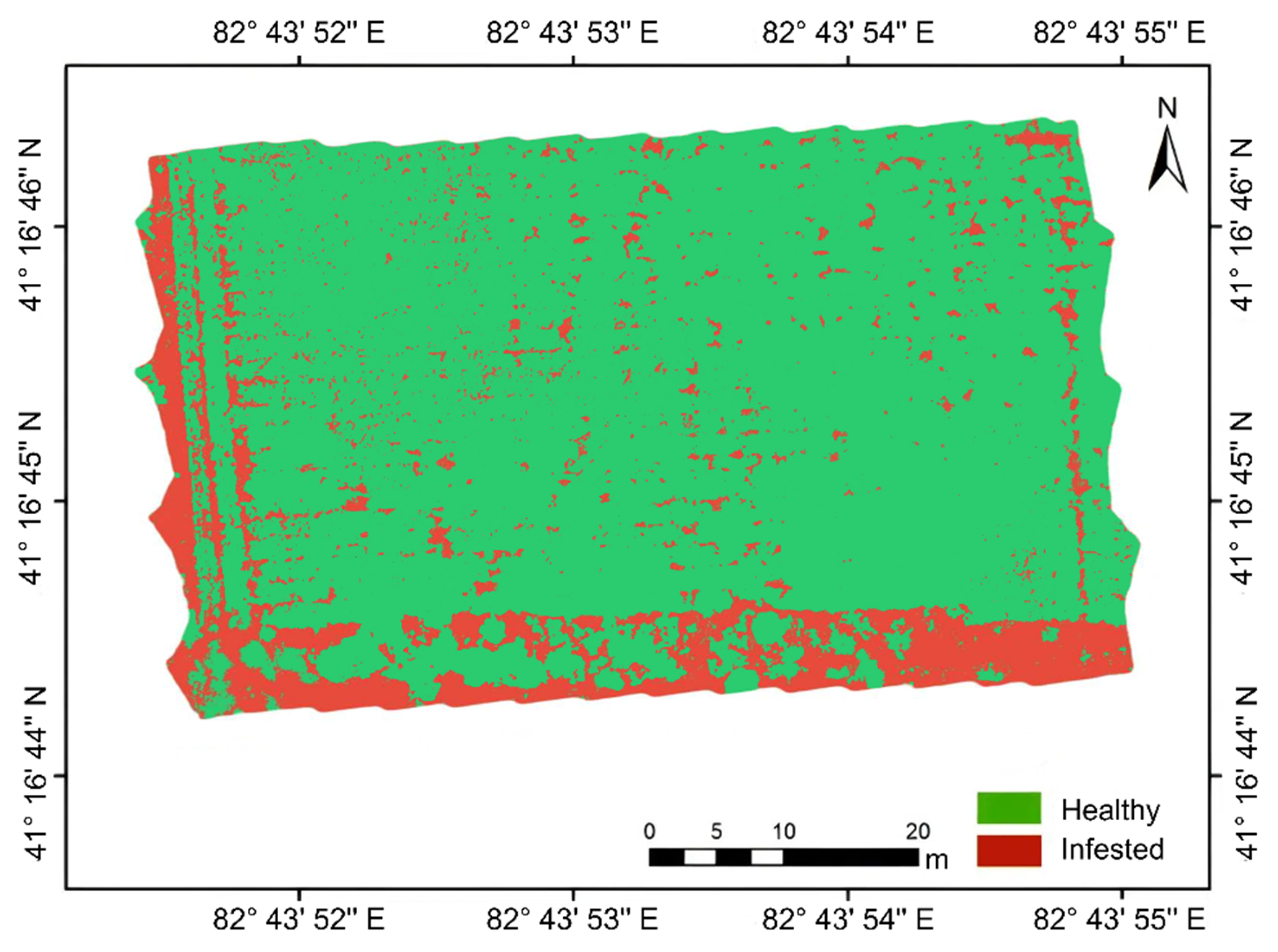
The selected RF model was subsequently applied to the entire study area using the four optimal vegetation indices (RDVI, MSAVI, SAVI, and OSAVI) to generate a centimeter-level spatial distribution map of mite occurrence (Figure 6). The resulting map clearly delineates infested areas (shown in red) from healthy areas (shown in green), providing precise guidance for targeted pesticide application.

2.5. Path Planning

Based on the spatial distribution map of mite damage and operational area statistics, this study directly converted identification results into path planning inputs. The mite distribution map was output in GeoTIFF format, containing the spatial position (longitude and latitude coordinates) and classification information (0 = healthy, 1 = mite-damaged) of each pixel, serving directly as input data for path planning. By counting the number of pixels classified as mite-damaged and combining with spatial resolution (1.1 cm), the operational area was automatically calculated, providing basic parameters for path optimization and pesticide dosage calculation.

2.5.1. Multi-Objective Path Planning Model

Plant protection UAV path planning is essentially a multi-objective optimization problem that requires seeking optimal balance among multiple mutually constraining performance indicators. Although traditional full-coverage path planning methods can achieve complete coverage of operational areas, they fail to consider the spatial distribution characteristics of pests and diseases, leading to substantial ineffective spraying. Precision variable-rate application based on mite identification results requires that path planning algorithms can automatically adapt to the geometric shapes of irregular operational areas while optimizing collaborative operation strategies for multiple UAVs. This study constructed a mathematical model containing 5 optimization objectives:

(1) Minimize deadheading distance (f₁): Non-operational flight distance, including total distance from takeoff to operational area, inter-area transfers, and return to base station. Reducing deadheading distance can improve operational efficiency and reduce time costs. (2) Minimize energy consumption (f₂): Battery energy consumption considering dynamic payload changes during flight operations. The energy model accounts for the continuous decrease in liquid pesticide load through a segment-based rate function r(L,m) that varies with remaining load L and flight mode m∈{idle, op}. Accurate energy modeling enables precise prediction of battery depletion and maximum operational area per sortie. (3) Minimize operation completion time (f₃): The longest time for all UAVs to complete all operational tasks, reflecting overall operational efficiency. For time-sensitive pest and disease control, shortening operation time can control disaster spread in a timely manner. (4) Minimize number of turns in flight path (f₄): Frequent turns reduce spray uniformity and increase risks of missed and repeated spraying, while energy consumption increases during turning. Reducing the number of turns helps improve application quality and reduce energy consumption. (5) Minimize multi-UAV load balance (f₅): The coefficient of variation CV = σ/μ is used to measure the dispersion of operation time among UAVs. Load balancing can avoid individual UAV overload or idleness, improving resource utilization efficiency.

The multi-objective optimization model can be expressed as

minimize: F(x) = [f₁(x), f₂(x), f₃(x), f₄(x), f₅(x)]^T

(5)

where x is the decision variable vector, including coverage angles of each operational area, path adjustment parameters, and UAV takeoff times. These 5 objectives have mutually constraining relationships: reducing the number of turns may increase deadheading distance, and shortening operation time may lead to load imbalance. Therefore, multi-objective optimization algorithms are needed to solve the Pareto optimal solution set, providing candidate solutions for multi-criteria decision-making.

Subject to constraints: (1) Endurance constraint: $L_{\mathit{single}}$ ≤ v × $T_{\mathit{max}}$ = 5400 m. (2) Coverage constraint: d ≤ W = 7 m. (3) Turning constraint: $r_{\mathit{turn} }$ ≥ $r_{\mathit{min}}$ = 4 m. (4) Boundary constraint: Path within operational area and avoiding obstacles. (5) Pesticide volume constraint: $V_i$ ≤ $V_{\mathit{tank}}$ = 30 L. (6) Time window constraint: operation completed within reasonable time to avoid environmental condition changes affecting effectiveness. These parameter values were determined based on DJI T30 technical specifications and field operational experience, with conservative margins applied for safety and reliability.

Among these objectives, the energy consumption model $f_2$ warrants detailed elaboration due to its critical role in determining operational capacity. The model is formulated as

$$f_2=\sum \left[r\right(L,m)·d]$$

(6)

where d is the segment length and the energy consumption rate r(L,m) is

$$r(L,m)=r_{base}\left(m\right)+\beta ·(L/L_{max})$$

(7)

where $r_{base}\left(m\right)$ represents the base energy rate for non-spraying flight (takeoff, return, inter-area transfer), β is the payload coefficient accounting for weight-induced energy increase, L is the current liquid pesticide load, and $L_{max}$ is the maximum tank capacity. The payload coefficient β captures the physical principle that heavier loads require greater lift force and thus higher energy consumption.

Meanwhile, for the coordinated coverage problem of multiple irregular operational areas, this study proposed a three-layer fusion optimization framework of “angle layer-path layer-scheduling layer.” By hierarchically decoupling decision variables at different scales, problem complexity is reduced.

The angle optimization layer determines the basic direction of parallel flight lines. Considering that cotton fields are mostly regularly planted with clear row directions, when the flight line direction aligns with the cotton planting row direction, the minimum number of flight lines and minimum boundary loss can be obtained. This layer adopted a heuristic initialization strategy based on Principal Component Analysis (PCA), extracting the first principal component direction of polygon vertices as the reference angle, with small random perturbations (±5°) added to maintain population diversity.

The path fine-tuning layer achieves fine adjustment of flight line positions through fine-tuning factor δ ∈ [−0.5, 0.5], with fine-tuning amount of δ × W (W is effective spray width). Its functions include: adapting to irregular boundary shapes to reduce boundary loss, obstacle avoidance, and optimizing overlap between adjacent flight lines to reduce re-spray rate.

The temporal scheduling layer decision variable is the takeoff time sequence t = [t₁, t₂, …, t_m] for m UAVs, where t_i ∈ [0, T_max] (T_max is maximum allowable delay time). This layer reduces extra energy consumption from mid-air collision avoidance maneuvers through staggered takeoffs and balances operational loads of each aircraft to prevent some UAVs from prematurely depleting battery.

The third layer variables are uniformly encoded as decision vector X = [θ₁…θ_n, δ₁…δ_n, t₁…t_m], with joint optimization achieved through multi-objective evolutionary algorithms, avoiding local optimum problems caused by inter-layer decoupling in traditional hierarchical methods.

2.5.2. Baseline Algorithm Comparison and Selection

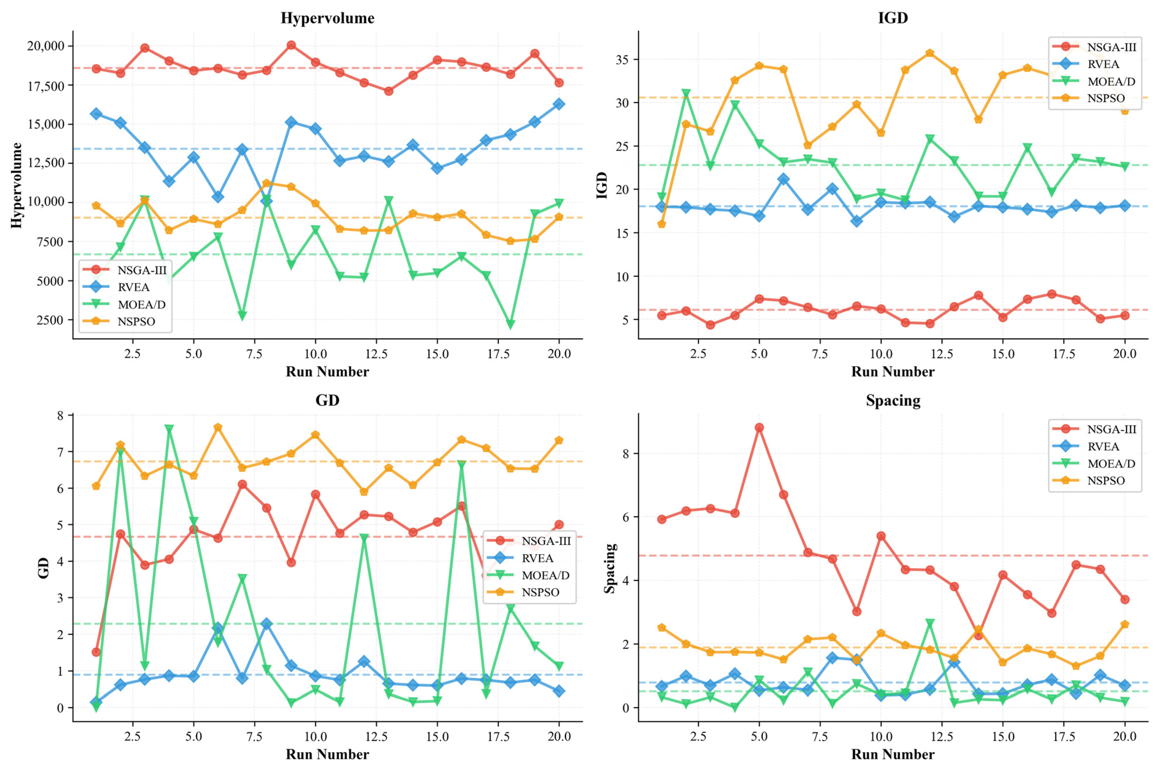
To select an optimization algorithm suitable for this problem, this study conducted systematic comparative experiments on 4 classic multi-objective evolutionary algorithms: NSGA-III, RVEA, MOEA/D, and NSPSO. These 4 algorithms represent different technical approaches in the field of multi-objective optimization: NSGA-III is based on non-dominated sorting and reference point mechanisms, suitable for handling multi-objective problems; RVEA uses reference vectors to guide evolutionary direction; MOEA/D decomposes multi-objective problems into multiple single-objective sub-problems; NSPSO combines Particle Swarm Optimization with non-dominated sorting. Experimental parameters were set as: population size of 100 individuals, evolution generations of 50, and 20 independent runs. Evaluation indicators adopted four standard performance metrics: Hypervolume (HV), Inverted Generational Distance (IGD), Generational Distance (GD), and Spacing. The performance indicator variation trends of each algorithm across 20 independent runs are shown in Figure 7. Statistical results are shown in

Table 5. Performance comparison of four multi-objective optimization algorithms.

Algorithm	HV	IGD	GD	Spacing
NSGA-III	18,581.76 ± 711.63	6.11 ± 1.08	4.66 ± 0.96	4.78 ± 1.51
RVEA	13,429.37 ± 1633.92	18.03 ± 1.03	0.88 ± 0.50	0.77 ± 0.36
MOEA/D	6669.25 ± 2325.80	22.78 ± 3.38	2.28 ± 2.48	0.50 ± 0.56
NSPSO	9018.96 ± 1000.17	30.57 ± 4.80	6.73 ± 0.48	1.88 ± 0.37

Note: HV, Hypervolume; IGD, Inverted Generational Distance; GD, Generational Distance. Higher HV and lower IGD/GD/Spacing indicate better performance. Mean ± SD from 20 independent runs. NSGA-III, Non-dominated Sorting Genetic Algorithm III; RVEA, Reference Vector-guided Evolutionary Algorithm; MOEA/D, multi-objective evolutionary algorithm based on Decomposition; NSPSO, Non-dominated Sorting Particle Swarm Optimization.

.

Comparative experiments showed that NSGA-III significantly outperformed other algorithms in the comprehensive indicators HV and IGD, with an HV value of 18,581.76 ± 711.63, 38.4% higher than second-place RVEA, and IGD value of 6.11 ± 1.08, only 33.9% of RVEA’s, indicating its obvious advantages in convergence and objective space coverage capability. Although RVEA performed better on the GD indicator (0.88 ± 0.50) and MOEA/D on the Spacing indicator (0.50 ± 0.56), the HV values of these two algorithms were only 72.3% and 35.9% of NSGA-III respectively, with obviously insufficient solution set quality. NSPSO achieved the worst IGD value (30.57 ± 4.80) among the four algorithms, indicating poor convergence quality.

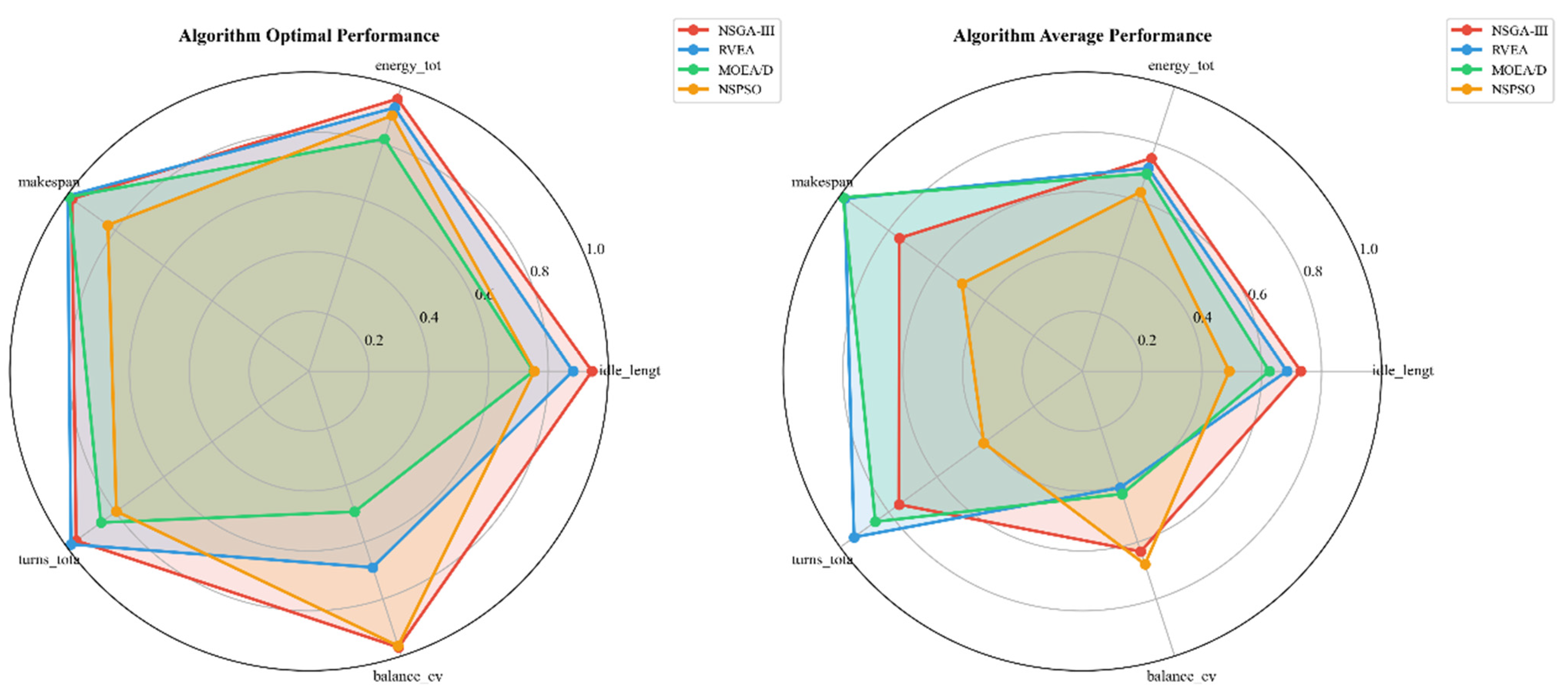
From the perspective of practical path planning applications, Figure 8 compares the performance of the 4 algorithms on 5 optimization objectives. From both optimal performance (left) and average performance (right) perspectives, NSGA-III significantly outperformed other algorithms on three key objectives: deadheading distance, energy consumption, and load balance. Although MOEA/D had a slight advantage in the number of turns, its performance on deadheading distance and energy consumption objectives was poor, with overall performance unsatisfactory. NSPSO performed acceptably on the makespan objective but was at a disadvantage on other objectives. RVEA’s comprehensive performance was intermediate but still had an obvious gap compared to NSGA-III.

Comprehensively evaluating both algorithm performance indicators and practical application objectives, NSGA-III demonstrated optimal performance in convergence, solution set quality, and optimization effectiveness for practical path planning. Therefore, this study selected NSGA-III as the baseline algorithm and subsequently improved its deficiencies in convergence speed and solution distribution uniformity.

2.5.3. Improved NSGA-III Algorithm

Building upon the NSGA-III basic framework, this paper addressed several limitations in the standard algorithm for cotton field plant protection path planning, including low initialization quality, weak local search capability, and parameter rigidity. Systematic improvements were made in four aspects: initial population generation, evolutionary operator design, mutation mechanism, and evolution strategy. These improvements collectively formed the CDPS-NSGA-III algorithm.

(1)

Heuristic Intelligent Initialization Mechanism

Standard NSGA-III uses random initialization to generate populations, not utilizing structural features of the problem, leading to slow convergence. For the path planning problem in this paper, decision variables represent coverage angles of each boundary region, which directly determine path shape and length. For convex polygon boundaries, when the traversal direction aligns with the polygon’s main direction, shorter paths can usually be obtained. This study proposed a heuristic sampling strategy based on Principal Component Analysis (PCA), integrating this geometric characteristic into the initialization process.

For a boundary polygon, calculate its centered coordinate matrix, where the centroid is the polygon center. Perform singular value decomposition on the matrix:

$$P = U{\displaystyle \sum }{V}^T$$

(8)

where U and V are orthogonal matrices from singular value decomposition, and ∑ is a diagonal matrix containing singular values. Extract the first principal component and calculate the principal direction angle:

$${\theta }_{\mathrm{principal} }= \arctan 2(v_{1,y},v_{1,x})$$

(9)

where $v_{1,x}$ and $v_{1,y}$ are the x and y components of the first principal component direction vector. Based on the extracted principal direction, the initial population adopts a mixed sampling strategy: 60% of individuals add Gaussian perturbations near the principal direction with perturbation intensity set to 15°; the remaining 40% use random sampling to maintain population diversity. This heuristic combined with random strategy both utilizes structural features of the problem to improve initial solution quality and avoids premature convergence through random components.

(2)

Differential Evolution Operator

To enhance global search capability and population diversity maintenance capability, this paper introduced the differential evolution (DE) operator to replace the SBX crossover operator in standard NSGA-III. The DE operator uses difference vectors between population individuals for mutation, with stronger ability to escape local optima. This paper adopted the DE/rand/1/bin strategy, with the mutation operation as

$$v_i={ x}_{r1}+F·(x_{r2} - x_{r3})$$

(10)

where v_i is the mutant vector, $x_{r1}$, $x_{r2}$, $x_{r3}$ are three randomly selected distinct individuals from the population (r1 ≠ r2 ≠ r3 ≠ i), and F is the scaling factor. Binomial crossover generates trial vectors:

$$u_{i,j}=\left\{\begin{array}{c}{v}_{i,j \mathit{if} \mathit{rand}\left(0,1\right) < \mathit{CR} \mathrm{or} j=j_{\mathit{rand}}} \\ {\mathrm{x}}_{\mathrm{i},\mathrm{j} \mathrm{otherwise}}\end{array}\right.$$

(11)

where u_i,j is the j-th component of the trial vector, v_i,j and x_i,j are the j-th components of the mutant and parent vectors respectively, CR is the crossover probability, and $j_{\mathit{rand}}$ is a randomly selected dimension. Based on literature recommendations and preliminary experimental tuning [40,41], F = 0.8 and CR = 0.9 were set. Analysis shows that the DE operator has stronger global exploration capability compared to the SBX operator. Let $D_{\mathit{pop}}$ denote the average Euclidean distance between population individuals. The SBX operator generates offspring primarily between parent solutions with expected distance approximately $D_{\mathit{pop}}/2$ from the population center, while the DE operator’s difference vector-based mutation mechanism (Equation (10)) produces trial vectors with substantially larger expected distances, typically exceeding $D_{\mathit{pop}}$ when F ≥ 0.5. With F = 0.8, the DE operator can explore a significantly larger range, effectively avoiding local optima.

(3)

Co-evolutionary Dual Population Strategy (CDPS)

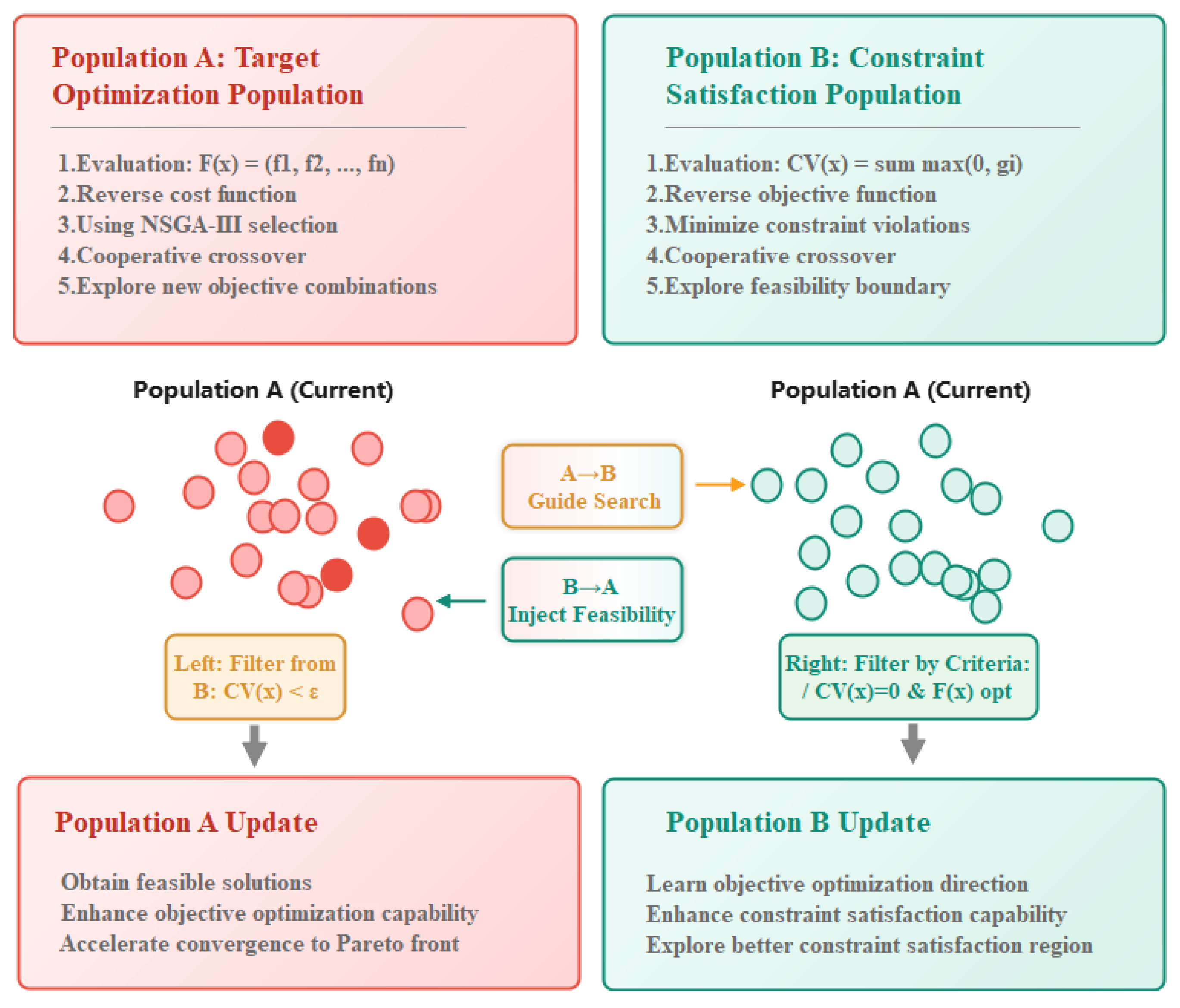
Addressing problems such as coupling conflicts between constraints and objectives and difficulty in obtaining feasible solutions, this paper proposed a co-evolutionary dual population strategy (CDPS). This strategy maintains two parallel evolving populations of equal size N: Population A focuses on optimizing objective function F(x), adopting NSGA-III selection mechanism, completely ignoring constraints; Population B focuses on minimizing constraint violation $C_{V\left(x\right)}$, selecting by $C_V$ ranking, completely ignoring objectives. Constraint violation is defined as

$$C_{V\left(x\right)}=\sum _{j=1}^J\mathit{max}\left(0,g_{j\left(x\right)}\right)+\sum _{k=1}^K\left|h_{k\left(x\right)}\right|$$

(12)

where J is the total number of inequality constraints, K is the total number of equality constraints, $g_{j\left(x\right)}$ ≤ 0 are inequality constraints, and $h_{k\left(x\right)}$ = 0 are equality constraints. When $C_{V\left(x\right)}$ = 0, the individual is completely feasible. The two populations achieve specialized search through functional separation: A explores Pareto front structure, B rapidly enters the feasible region. The process is shown in Figure 9.

To select the final solution from the Pareto optimal set for practical implementation, a fuzzy membership function-based decision-making method was adopted. For each objective $f_i$, the membership value ${\mu }_i$ was calculated as

$${\mu }_i={\displaystyle \frac{f_i^{max}-f_i}{f_i^{max}-f_i^{min}}}$$

(13)

where $f_i^{max}$ and $f_i^{min}$ represent the maximum and minimum values of the i objective across all Pareto solutions. The comprehensive satisfaction degree for each solution was computed as the average of all membership values, and the solution with the highest comprehensive satisfaction degree was selected as the final execution scheme.

Knowledge transfer mechanism: Bidirectional migration is performed every T = 10 generations. A → B migration set is defined as

$$S_{\left\{A\to B\right\}}=\left\{x\in P_A|C_{V\left(x\right)} < \epsilon \right\}$$

(14)

where $\epsilon$ = 0.1 is the feasibility threshold. This migration injects “nearly feasible” high-quality solutions from population A into B, accelerating convergence toward high-quality regions within the feasible domain. B → A migration set is defined as

$$S_{\left\{B\to A\right\}}=\left\{x\in P_B|C_{V\left(x\right)}=0\right\}$$

(15)

This migration injects feasible solutions from population B into A, enabling A to produce new offspring around feasible solutions. To verify the theoretical effectiveness of CDPS, this paper provided the following convergence theorem: If population $P_B$ converges to the feasible region with probability 1, then through B → A migration, population $P_A$ includes feasible solutions with probability 1; the expected generations for CDPS to obtain feasible solutions is less than single-population NSGA-III. The above theorem indicates that the dual population co-evolutionary mechanism not only theoretically guarantees acquisition of feasible solutions but also has faster convergence speed compared to single-population algorithms.

Building on CDPS, to further enhance information exchange between populations, this paper introduced a co-evolutionary crossover strategy: when generating offspring, populations select crossover parents across populations with probability ${\mathrm{p}}_{\mathrm{c}}$ = 0.3 to enhance information exchange. This probability value was determined through preliminary experimental tuning, ensuring information exchange while avoiding loss of population characteristics due to excessive mixing. Population A selects low CV individuals from B to obtain feasibility, and B selects individuals with good objectives from A to balance performance. Combined with the differential evolution operator (Equation (8)), parents can come from different populations. Environmental selection: Population A adopts NSGA-III selection (non-dominated sorting + reference point association), completely ignoring CV; Population B ranks by CV in ascending order and selects the top N individuals, completely ignoring F.

Complexity analysis: Although maintaining two populations, the size of a single population is N (not 2N), and selection operations can be executed in parallel. The time complexity per generation is

$$T_{\mathit{single}}=O\left({\mathit{MN}}^2+\mathit{NM}\left|Z\right|\right)=O\left({\mathit{MN}}^2\right)$$

(16)

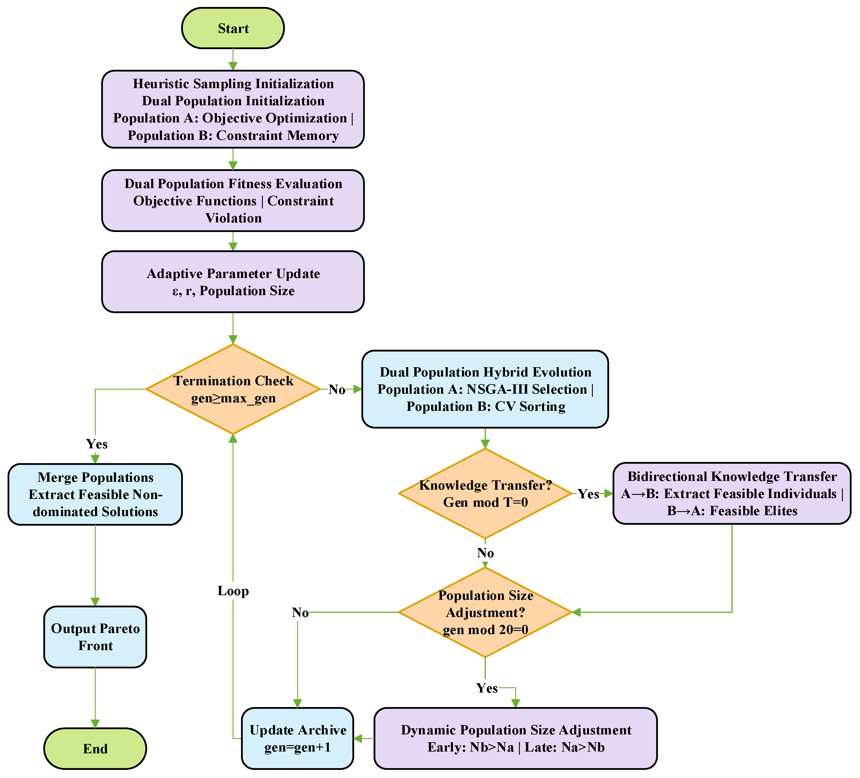
where M is the number of objectives (M = 5), N is the population size, |Z| is the number of reference points, D is the decision variable dimension, and G is the number of generations. Same as standard NSGA-III. Total time complexity is O(${MN}^2$G), and Space complexity is O(2N$·$D + |Z|M), approximately twice that of standard NSGA-III but acceptable. The complete algorithm flow is shown in Figure 10.

3. Results and Discussion

3.1. Mite Damage Identification Results

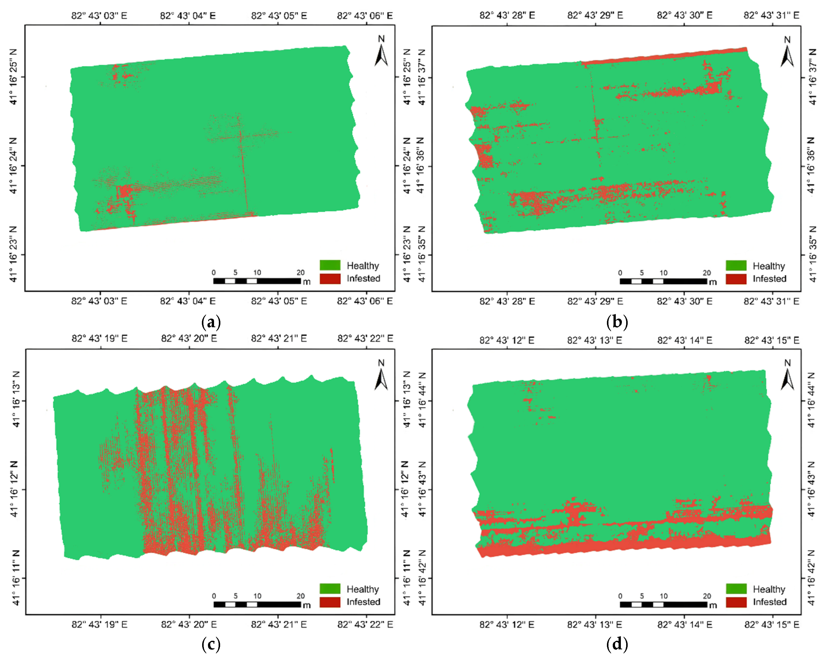
This study conducted mite damage identification experiments in four cotton field plots in Shaya County, Xinjiang. Plots 1, 2, and 3 planted the Xinluzhong 80 variety with a one-film-six-row planting pattern; Plot 4 planted the Yuanmian 11 variety with a one-film-three-row planting pattern. The Random Forest constructed based on RDVI, MSAVI, SAVI, and OSAVI was applied to the four plots to generate spatial distribution maps of mite damage (Figure 11a–d), and identification results were validated with ground surveys. Specific conditions of the four plots are shown in

Table 6. Mite damage identification results and accuracy in experimental sites.

Plot	Location	Variety	Planting Pattern	Survey Points	Infestation Rate (%)	Accuracy (%)
1	Alfalfa shelterbelt	Xinluzhong 80	One-film-six-row	195	28	85.24
2	Alfalfa shelterbelt	Xinluzhong 80	One-film-six-row	86	36	86.51
3	Rapeseed shelterbelt	Xinluzhong 80	One-film-six-row	92	45	83.90
4	Hailou District 1	Yuanmian 11	One-film-three-row	68	39	79.73

Note: Plots 1–3 planted Xinluzhong 80 variety with one-film-six-row pattern; Plot 4 planted Yuanmian 11 variety with one-film-three-row pattern. Accuracy calculated as agreement between model predictions and ground survey results.

. The spatial distribution of mite occurrence is shown in Figure 11.

According to the results, all four plots exhibited varying degrees of mite occurrence, with infestation rates ranging from 28% to 45%, averaging 37%. Plot 3 had the most severe mite occurrence (45%), Plot 1 the lightest (28%), and Plots 2 and 4 were 36% and 39% respectively. From spatial distribution perspectives (Figure 11), Plot 1 showed scattered patchy mite damage, mainly concentrated in the center and edges; Plot 2 exhibited strip distribution along the northern edge; Plot 3 showed field-wide scattered distribution, with obvious mite damage in the southern area near roads with weeds, scattered patches in the center, and east–west boundaries; Plot 4 showed concentrated occurrence in the south and relatively sparse in the north.

The model achieved an average accuracy of 83.85% across the four plots. Plot 2 had the highest accuracy (86.51%), and Plot 4 the lowest (79.73%). Plots 1 and 2 (Xinluzhong 80) both exceeded 85% accuracy, demonstrating that the Random Forest based on vegetation indices RDVI, MSAVI, SAVI, and OSAVI can effectively identify cotton field mite damage. Plot 3 (same variety Xinluzhong 80) had an accuracy of 83.90%, a decrease of 2.61 percentage points compared to Plot 2, but still maintained high performance. This plot had the highest infestation rate (45%) with roadside weed area interference in the south. Despite different environmental conditions and mite occurrence levels, the model could still accurately capture the spatial distribution pattern of mite damage. Plot 4 (Yuanmian 11) showed decreased accuracy to 79.73%, a reduction of 5.49 percentage points compared to the same-variety plot average (85.22%). The main reasons for accuracy reduction include: spectral differences between varieties, with Yuanmian 11 having thinner leaves and lighter color; planting pattern effects, where the one-film-three-row pattern has larger row spacing, enhancing soil background interference. The model successfully identified the main mite damage area in the south, demonstrating certain cross-variety applicability. Subsequently, model universality can be further improved by expanding training samples with different varieties and planting patterns.

The observed performance variation across varieties warrants further mechanistic interpretation. The spectral characteristics of cotton canopy are fundamentally determined by leaf biochemical composition and canopy architecture. Yuanmian 11, as a hybrid variety, may exhibit different canopy structural and biochemical characteristics compared to Xinluzhong 80, which could influence spectral reflectance patterns in the red-edge and near-infrared regions critical for Vegetation Index calculation [42]. Furthermore, the one-film-three-row planting pattern adopted for Yuanmian 11 results in approximately 40% greater row spacing, which increases the proportion of exposed soil background in mixed pixels and consequently affects the sensitivity of vegetation indices to subtle stress-induced spectral changes. These factors collectively contribute to the observed accuracy reduction for Yuanmian 11, highlighting the importance of variety-specific model calibration in future applications.

3.2. Path Planning Results

Based on the mite damage identification results from the Plot 1 experimental site (2180 m² operational area), this section demonstrated the optimization process of the multi-objective path planning module and the precision variable-rate application effect.

3.2.1. Mite Area Preprocessing and Parameter Settings

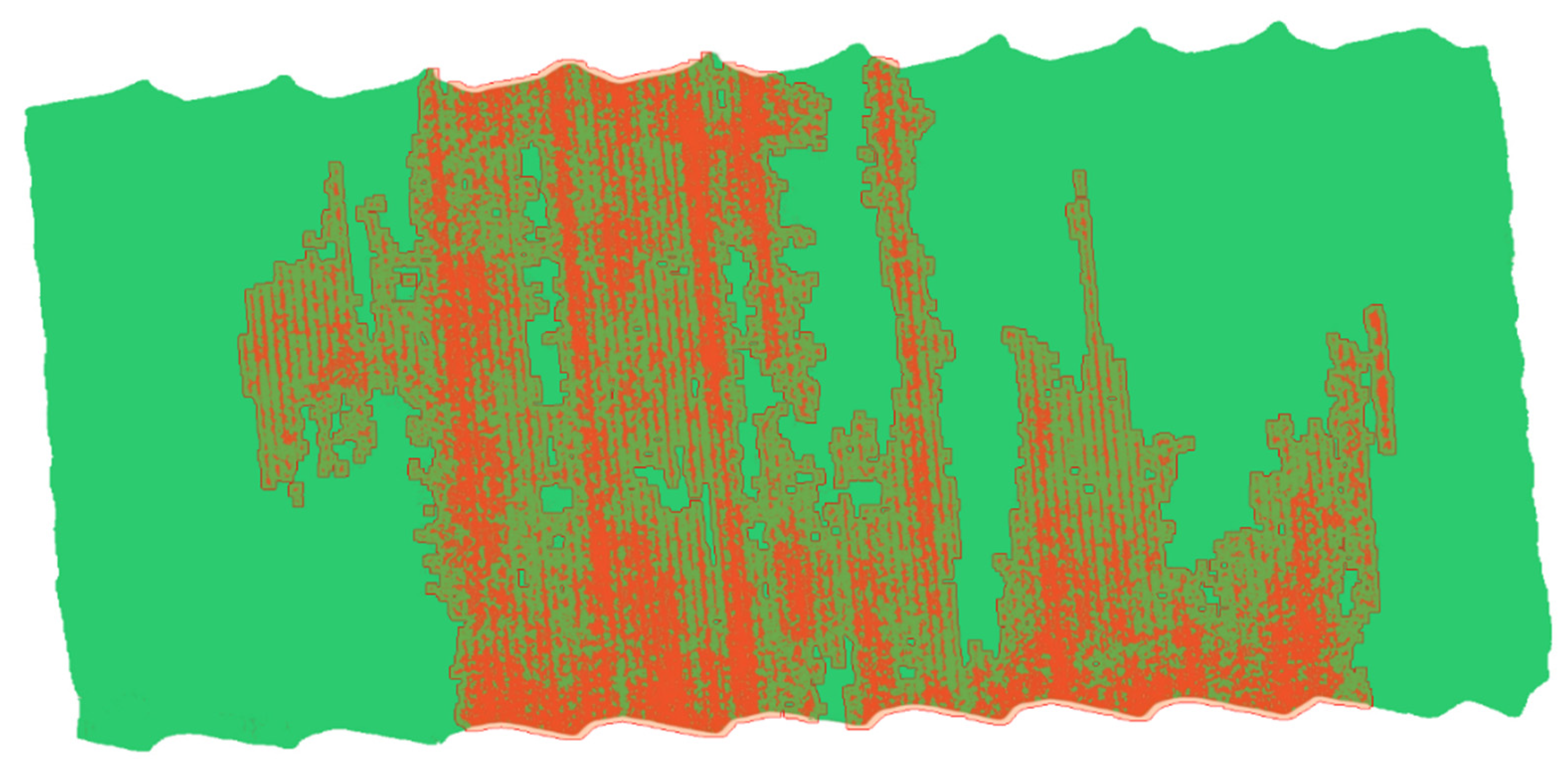
Morphological dilation processing was performed on the identified mite distribution map (Figure 12) to prevent missed spraying. A circular structuring element with radius 3.5 m (0.5× the UAV spray width of 7 m) [43,44]. This ratio accounts for GPS positioning uncertainty, spray drift (typically 0.4–0.6× spray width under field conditions), and potential mite movement at infestation edges. The 0.5× ratio balances coverage completeness against overspraying: smaller ratios risk missed areas, while larger ratios increase unnecessary pesticide use. Cotton spider mites primarily disperse through ambulatory movement (crawling) over short distances, while wind-assisted aerial migration serves as a secondary mechanism for longer-distance dispersal. Within the operational window (3–6 h from image acquisition to spraying), the 3.5 m buffer provides adequate margin to account for local colony boundary shifts, while also capturing adjacent susceptible zones where early-stage damage may exist below the multispectral detection threshold. To ensure system reliability under field conditions, a 4G/5G cellular network was used for UAV-ground station communication with automatic mission replay capability in case of signal interruption, while RTK-GPS provided positioning accuracy sufficient for the designed buffer margin and a safety buffer while maintaining precision agriculture efficiency. Connected component analysis (8-neighborhood) was performed on the dilated area, Geometric parameters of each patch (centroid coordinates, area, perimeter, major and minor axes, orientation angle) were extracted to provide inputs for path planning.

3.2.2. Multi-Objective Optimization Results

To verify the effectiveness of the improved NSGA-III algorithm and quantify the contribution of each improvement component, this study designed path planning test scenarios based on the mite distribution map obtained in Section 3.1. An ablation study was conducted by incrementally adding each component: PCA-based initialization, DE operator, and CDPS. Four indicators—HV, IGD, GD, and Spacing—were used to evaluate algorithm performance, with each configuration independently run 20 times and averaged, with 100 generations per run. Results are shown in

Table 7. Ablation study of the improved NSGA-III algorithm.

Configuration	HV	IGD	GD	Spacing
NSGA-III	41,000.40	2.92	2.70	1.63
+ PCA Initialization	41,736.33	2.72	2.82	1.77
+ DE Operator	42,575.20	1.69	2.53	1.65
+ CDPS	43,417.46	1.17	2.31	1.40

Note: Mean ± SD from 20 runs. PCA, Principal Component Analysis; DE, differential evolution; CDPS, co-evolutionary dual population strategy; HV, Hypervolume; IGD, Inverted Generational Distance; GD, Generational Distance. Higher HV and lower IGD/GD/Spacing indicate better performance.

.

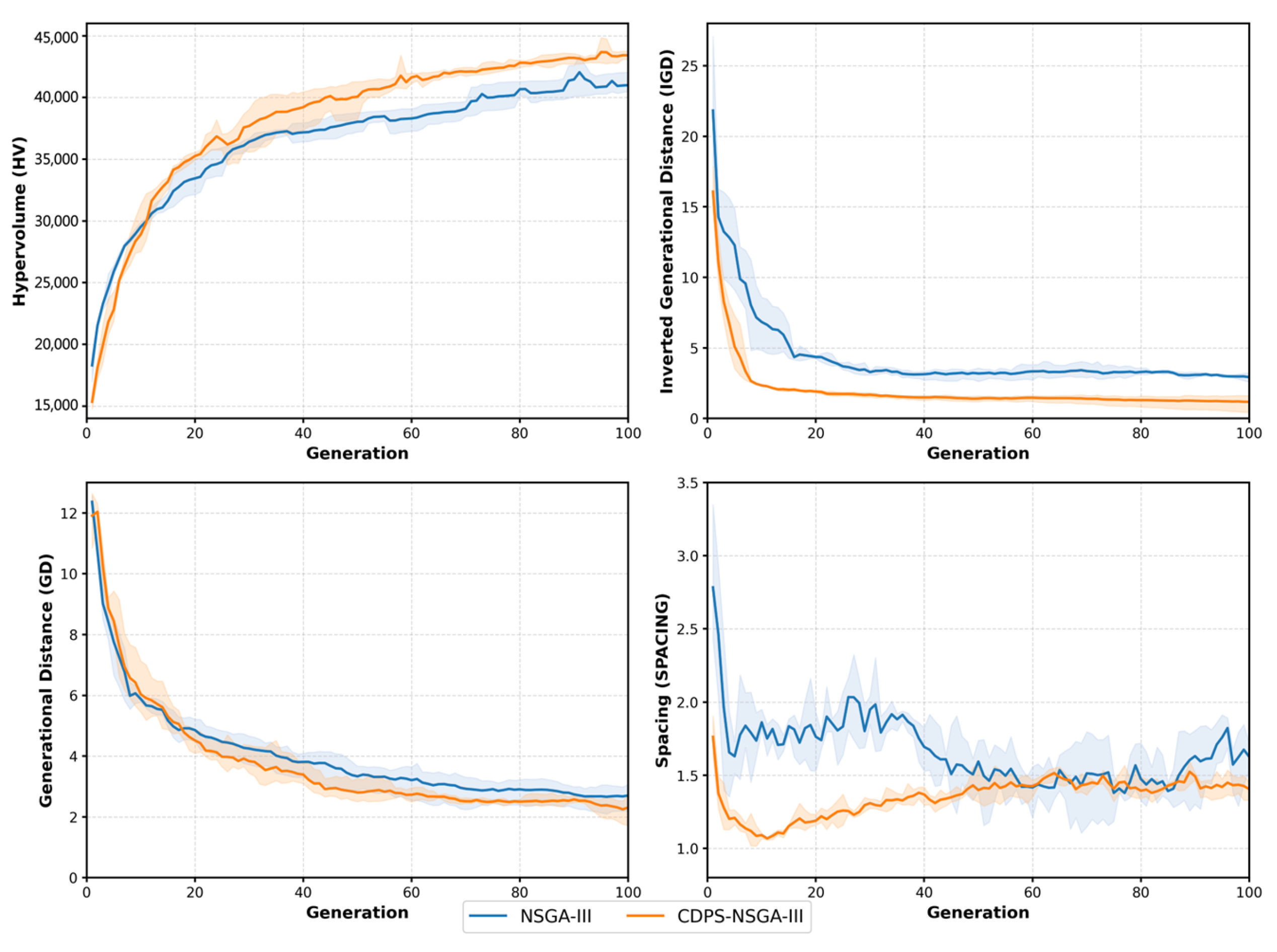
Results showed that the improved algorithm (CDPS-NSGA-III) achieved significant improvements across all four indicators. IGD decreased from 2.92 to 1.17, a reduction of 59.94%, indicating that the solution set was closer to the true Pareto front; Spacing decreased from 1.63 to 1.40, a reduction of 14.11%, with more uniform solution distribution; HV increased from 41,000.40 to 43,417.46, an increase of 5.90%, with significantly improved convergence quality; GD decreased from 2.70 to 2.31, a reduction of 14.44%. The ablation study revealed the functional roles of each component: PCA initialization accelerated convergence by guiding the population toward promising regions (HV and IGD improved), though with a temporary trade-off in diversity; DE operator subsequently restored global search capability; and CDPS ultimately balanced both convergence and uniformity. Overall, the improved algorithm outperformed standard NSGA-III in convergence, uniformity, and solution set quality.

3.2.3. Convergence Characteristic Analysis

In addition to final performance, algorithm convergence speed also affects practical application efficiency. Figure 13 records the dynamic change trajectories of the four performance indicators for both algorithms over 100 generations of evolution. From convergence curves, it can be observed that the CDPS-NSGA-III demonstrated faster convergence speed and better final performance on the two core indicators HV and IGD: the HV curve rose rapidly in the first 20 generations, reaching the level of the original algorithm’s 100 generations around generation 15; the IGD curve dropped sharply in the first 10 generations, stabilizing below 0.1 after generation 20, while the original algorithm’s IGD value stabilized around 0.15 throughout the evolution process. The improved algorithm, through faster convergence speed and better final solution quality, can significantly reduce path planning computation time in practical applications.

Regarding the GD indicator, both algorithms showed similar convergence trends, rapidly decreasing from initial high values and trending toward stability, However, CDPS-NSGA-III exhibited a smoother curve with smaller fluctuation amplitude, finally stabilizing around 2.3, slightly better than the original algorithm’s 2.7. This reflects the role of differential evolution operators and adaptive mutation mechanisms in stabilizing the convergence process. The Spacing indicator comparison was more obvious: the proposed method could rapidly establish a uniformly distributed solution set in early evolution (within approximately 10 generations) and maintain stability in subsequent evolution, with the curve consistently maintained around 1.40; while the original algorithm consistently showed large fluctuations, oscillating violently between 1.5 and 2.0, indicating difficulty in simultaneously balancing solution quality and distribution uniformity.

Comprehensive performance analysis showed that through the synergistic effects of heuristic initialization, differential evolution operators, and co-evolutionary dual population strategies, the improved NSGA-III algorithm significantly improved solution set distribution uniformity, algorithm stability, and convergence speed while maintaining high-quality Pareto fronts, providing reliable technical support for subsequent precision application path planning.

3.2.4. Practical Path Planning Results

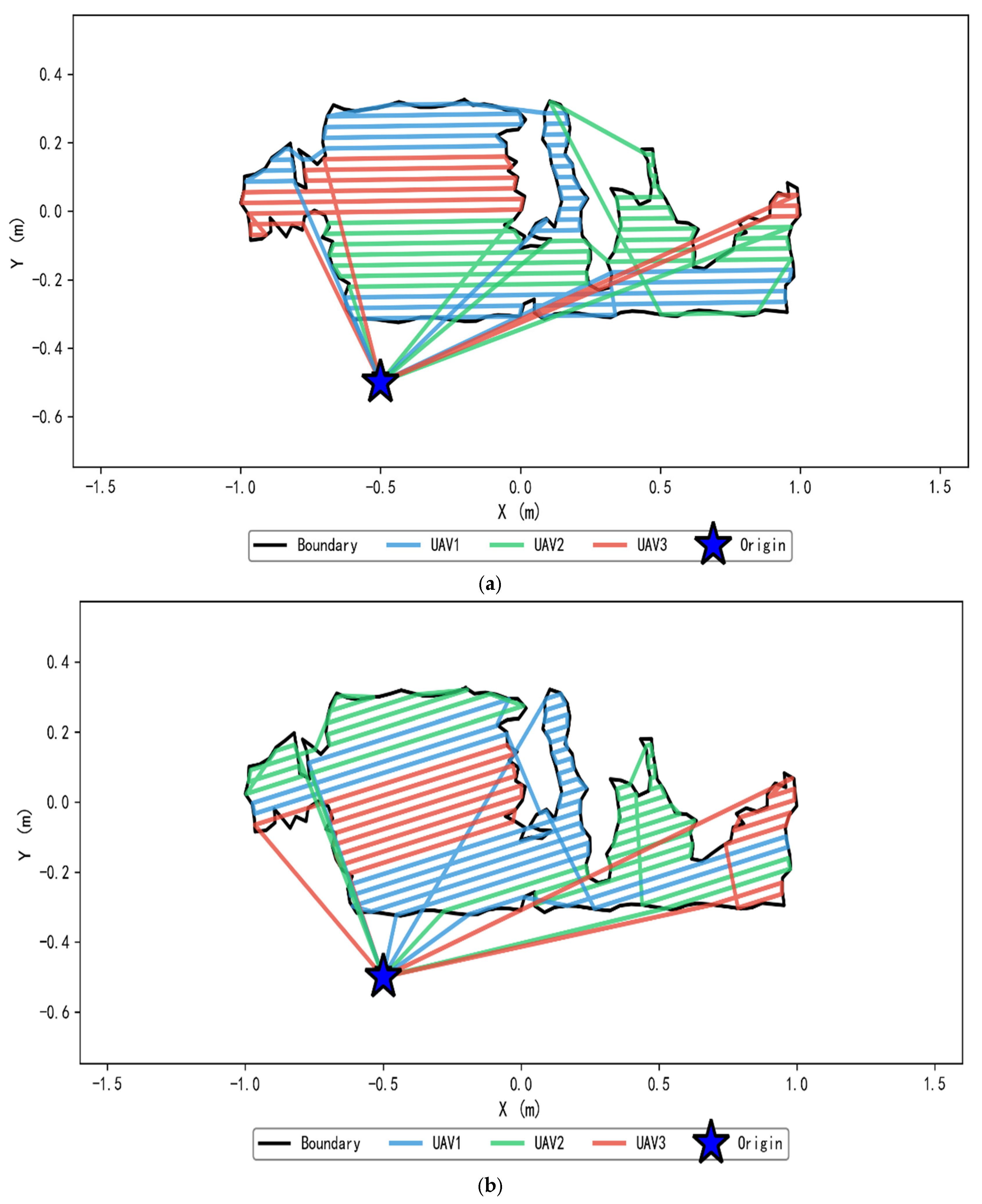
To intuitively demonstrate the advantages of the improved algorithm in practical applications, Figure 14 compares optimal path solutions generated by the two algorithms. Based on the mite distribution map of the Plot 1 experimental site (operational area 2750 m²), 3 plant protection UAVs were used for coordinated operations. Comparative analysis was conducted from two perspectives: path planning top view and total path length of each UAV. Figure 14a shows the original NSGA-III algorithm, and Figure 14b shows the improved algorithm.

From path planning effectiveness, the improved algorithm achieved significant improvements in multiple key indicators (

Table 8. Path planning results of NSGA-III algorithm before and after improvement.

Evaluation Metric	NSGA-III	CDPS-NSGA-III	Improvement
Coverage rate (%)	97.2	98.5	1.3%
Path overlap rate (%)	9.2	3.6	−60.9%
Total path length (m)	501.4	483.2	−3.6%
Longest path (m)	177.1	157.9	−10.8%
Shortest path (m)	85.6	93.3	+9.0%

Note: Three DJI T30 UAVs with 7 m spray width operating at 5 m/s flight speed. Coverage rate, percentage of target area covered; overlap rate, percentage of area with redundant coverage; total path length includes all operational and deadheading segments.

). In terms of coverage rate, the improved algorithm reached 98.5%, a 1.3 percentage point improvement compared to the standard algorithm’s 97.2%, better ensuring complete coverage of mite-damaged areas. Path overlap rate decreased from 9.2% to 3.6%, a reduction of 60.9%, effectively avoiding pesticide waste and crop phytotoxicity risks caused by repeated spraying. Calculated at a unit area pesticide application rate of 80 g/ha, the reduction in path overlap rate from 9.2% to 3.6% can reduce pesticide waste by approximately 448 g per 100 ha (0.45 kg per 100 ha), representing significant economic benefits in large-scale applications.

Total path length was optimized from 501.4 m to 483.2 m. Although the improvement was only 3.6%, combined with the substantial reduction in path overlap rate, the actual effective spraying path was more precise. For a single plant protection UAV with an average flight speed of 5 m/s, path optimization can save operation time, significantly improving overall efficiency and extending flight range in multi-plot continuous operations.

Path quality analysis further validated the advantages of the improved algorithm. From the top view, it can be observed that paths generated by the standard algorithm had more crossings and overlaps (intersection areas of different colored stripes), with particularly unreasonable deadheading path planning between two mite-damaged areas. Some boundary areas showed coverage gaps due to improper path coverage angles (upper left and central areas). Paths generated by the improved algorithm were more regular, with uniform spacing between flight lines and smoother turn connections. Path directions better matched the boundaries of mite-damaged areas, reflecting the role of PCA heuristic initialization in optimizing coverage angles. Path allocation of UAV2 and UAV3 in the right mite-damaged area was more reasonable, avoiding the problem of UAV2 overload in the standard algorithm.

Overall, the improved NSGA-III algorithm significantly reduced path overlap rate (reduction of 60.9%) while ensuring high coverage (98.5%), providing an efficient and economical path planning solution for multi-UAV coordinated precision application, achieving unity of economic and ecological benefits while ensuring control effectiveness.

4. Conclusions

This study addressed the practical needs for precision cotton field mite damage control and constructed a complete technical system for intelligent mite monitoring and precision pesticide application based on UAV multispectral remote sensing, achieving full-chain technological innovation from identification to application. The main conclusions were as follows:

(1)

In mite damage identification, through combined preprocessing of Savitzky–Golay smoothing filtering and Multiplicative Scatter Correction, the spectral separability between healthy and damaged cotton plants was effectively enhanced, achieving optimal discrimination in the near-infrared band. Based on the Bayesian Information Criterion, RDVI, MSAVI, SAVI, and OSAVI were selected from 14 vegetation indices as the optimal feature set. Five classification models were evaluated, including three machine learning methods (Logistic Regression, Random Forest, and Support Vector Machine) and two deep learning architectures (1D-CNN and MobileNetV2). While deep learning models achieved marginally higher accuracy, their computational cost was significantly greater. Balancing classification performance and real-time processing requirements for UAV deployment, Random Forest was selected as the optimal model, achieving 85.47% accuracy on the validation set with an F1-score of 85.24%, validating the model’s good generalization ability. The model successfully generated centimeter-level spatial distribution maps of mite damage, providing reliable basis for precisely delineating pesticide application areas. Cross-plot validation across four experimental plots with two varieties and two planting patterns achieved an average accuracy of 83.85%. Under the same variety and planting pattern conditions, model accuracy remained above 85%, while cross-variety application showed reduced accuracy (79.73%), indicating potential for further improvement through expanded training samples.

(2)

In path planning, to address problems in the standard NSGA-III algorithm for cotton field variable-rate application scenarios such as low initialization quality and weak local search capability, three systematic improvements were proposed: first, introducing PCA heuristic initialization to leverage geometric features of mite-damaged areas to improve initial population quality; second, adopting differential evolution operators to enhance global search capability; third, constructing a co-evolutionary dual population strategy to accelerate feasible solution acquisition. Ablation study demonstrated that each component contributed to performance improvement: PCA initialization accelerated convergence, DE operator enhanced global search capability, and CDPS balanced convergence and diversity. The fully improved algorithm achieved significant gains over standard NSGA-III: IGD decreased by 59.94%, HV increased by 5.90%, Spacing decreased by 14.11%, and GD decreased by 14.44%, with significant improvements in both convergence speed and solution set quality.

(3)

Field application validation showed that the technical solution achieved 98.5% coverage of mite-damaged areas in the experimental plot, with path overlap rate decreasing from 9.2% to 3.6%, and total path length optimized by 3.6% (from 501.4 m to 483.2 m). Compared to traditional field-wide spraying, this solution significantly reduced pesticide usage, operation time, and energy consumption, while avoiding non-target area pollution and protecting natural enemy populations such as ladybugs and lacewings, achieving synergistic economic and ecological benefits.

This study still has some limitations that warrant further investigation: (1) The current study was conducted in a single geographic region (Shaya County, Xinjiang) during a limited temporal window (July–August), corresponding only to the flowering and boll formation stage. The model’s applicability to other phenological stages, diverse climatic conditions, different soil types, and concurrent stress scenarios (e.g., combined mite infestation and water stress) remains to be validated. Future work could introduce multi-temporal monitoring across the full growth period to improve early warning capability and model robustness. (2) The model demonstrated sensitivity to varietal and planting pattern differences, with accuracy declining by 5.49 percentage points for Yuanmian 11 compared to Xinluzhong 80. Expanding training datasets to include additional cotton varieties and planting configurations would enhance cross-variety transferability. (3) The ROI-based approach primarily utilizes spectral characteristics rather than spatial texture features; future research could explore lightweight 2D architectures or texture indices to capture spatial patterns of mite damage. (4) The current system assumes a single pest scenario. In practice, cotton fields may experience multiple concurrent pest infestations (e.g., aphids, bollworms) requiring different pesticides and spray strategies. Future work could extend the framework to multi-pest detection and adaptive spraying protocols.

References

1. World Trade Organization. WTO Members Call for Urgent Action on Cotton Trade Challenges [EB/OL]. Available online: https://www.wto.org/english/news_e/news24_e/cott_29nov24_e.htm (accessed on 29 November 2024).
2. Feng, L.; Wan, S.; Zhang, Y.; Dong, H. Xinjiang cotton: Achieving super-high yield through efficient utilization of light, heat, water, and fertilizer by three generations of cultivation technology systems. Field Crop Res. 2024, 312, 109401. [Google Scholar] [CrossRef]
3. Jakubowska, M.; Dobosz, R.; Zawada, D.; Kowalska, J. A Review of Crop Protection Methods against the Twospotted Spider Mite—Tetranychus urticae Koch (Acari: Tetranychidae)—With Special Reference to Alternative Methods. Agriculture 2022, 12, 898. [Google Scholar] [CrossRef]
4. Chen, Y.; Nguyen, D.T.; Wheeler, D.; Herron, G.A. A novel mutation in mitochondrial cytochrome b conferring resistance to bifenazate in two-spotted spider mite Tetranychus urticae Koch (Acarina: Tetranychidae). Pest Manag. Sci. 2024, 80, 3612–3619. [Google Scholar] [CrossRef] [PubMed]
5. Han, Y.; Zhang, Y.-C.; Ye, W.-N.; Wang, S.-M.; Wang, X.; Gao, C.-F. Increasing resistance of Tetranychus urticae to common acaricides in China and risk assessment to spiromesifen. Crop Prot. 2024, 176, 106519. [Google Scholar] [CrossRef]
6. Weiss, M.; Jacob, F.; Duveiller, G. Remote sensing for agricultural applications: A meta-review. Remote Sens. Environ. 2020, 236, 111402. [Google Scholar] [CrossRef]
7. Wu, B.; Zhang, M.; Zeng, H.; Tian, F.; Potgieter, A.B.; Qin, X.; Yan, N.; Chang, S.; Zhao, Y.; Dong, Q.; et al. Challenges and opportunities in remote sensing-based crop monitoring: A review. Natl. Sci. Rev. 2023, 10, nwac290. [Google Scholar] [CrossRef]
8. Shahi, T.B.; Xu, C.-Y.; Neupane, A.; Guo, W. Recent advances in crop disease detection using UAV and deep learning techniques. Remote Sens. 2023, 15, 2450. [Google Scholar] [CrossRef]
9. Guebsi, R.; Mami, S.; Chokmani, K. Drones in precision agriculture: A comprehensive review of applications, technologies, and challenges. Drones 2024, 8, 686. [Google Scholar] [CrossRef]
10. Wang, J.; Zhang, S.; Lizaga, I.; Zhang, Y.; Ge, X.; Zhang, Z.; Zhang, W.; Huang, Q.; Hu, Z. UAS-based remote sensing for agricultural Monitoring: Current status and perspectives. Comput. Electron. Agric. 2024, 227, 109501. [Google Scholar] [CrossRef]
11. Berger, K.; Machwitz, M.; Kycko, M.; Kefauver, S.C.; Van Wittenberghe, S.; Gerhards, M.; Verrelst, J.; Atzberger, C.; van der Tol, C.; Damm, A.; et al. Multi-sensor spectral synergies for crop stress detection and monitoring in the optical domain: A review. Remote Sens. Environ. 2022, 280, 113198. [Google Scholar] [CrossRef]
12. Haq, S.I.U.; Wang, G.; Khan, S.N.; Song, C.; Ma, C.; Zhang, X.; Lan, Y. Multi-Dimensional Optical Remote Sensing in Agriculture: Spectral, Angular, and Spatial Scaling for Crop Stress Monitoring. Smart Agric. Technol. 2025, 12, 101583. [Google Scholar] [CrossRef]
13. Wu, Y.; Li, X.; Zhang, Q.; Zhou, X.; Qiu, H.; Wang, P. Recognition of spider mite infestations in jujube trees based on spectral-spatial clustering of hyperspectral images from UAVs. Front. Plant Sci. 2023, 14, 1078676. [Google Scholar] [CrossRef] [PubMed]
14. Yamada, M.; Thiesen, L.V.; Filho, F.H.I.; Yamamoto, P.T. Hyperspectral Imaging and Machine Learning: A Promising Tool for the Early Detection of Tetranychus urticae Koch Infestation in Cotton. Agriculture 2024, 14, 1573. [Google Scholar] [CrossRef]
15. Zhu, H.; Lin, C.; Liu, G.; Wang, D.; Qin, S.; Li, A.; Xu, J.-L.; He, Y. Intelligent agriculture: Deep learning in UAV-based remote sensing imagery for crop diseases and pests detection. Front. Plant Sci. 2024, 15, 1435016. [Google Scholar] [CrossRef]
16. García-Munguía, A.; Guerra-Ávila, P.L.; Islas-Ojeda, E.; Flores-Sánchez, J.L.; Vázquez-Martínez, O.; García-Munguía, A.M.; García-Munguía, O. A Review of drone technology and operation processes in agricultural crop spraying. Drones 2024, 8, 674. [Google Scholar] [CrossRef]
17. Nahiyoon, S.A.; Ren, Z.; Wei, P.; Li, X.; Li, X.; Xu, J.; Yan, X.; Yuan, H. Recent development trends in plant protection UAVs: A journey from conventional practices to cutting-edge technologies—A comprehensive review. Drones 2024, 8, 457. [Google Scholar] [CrossRef]
18. Choton, J.C.; Hsu, W.H. Coverage Path Planning in Precision Agriculture: Algorithms, Applications, and Key Benefits. arXiv 2024, arXiv:2412.19813. [Google Scholar] [CrossRef]
19. Li, W.; Luo, Y.; Jiang, P.; Dong, X.; Tang, K.; Liang, Z.; Shi, Y. A sustainable crop protection through integrated technologies: UAV-based detection, real-time pesticide mixing, and adaptive spraying. Sci. Rep. 2025, 15, 35748. [Google Scholar] [CrossRef]
20. Guo, Z.; Cai, D.; Bai, J.; Xu, T.; Yu, F. Intelligent rice field weed control in precision agriculture: From weed recognition to variable rate spraying. Agronomy 2024, 14, 1702. [Google Scholar] [CrossRef]
21. Liu, X.; Liu, Y.; Chen, X.; Wan, Y.; Gao, D.; Cao, P. LiDAR-assisted UAV variable-rate spraying system. Agriculture 2025, 15, 1782. [Google Scholar] [CrossRef]
22. Tuenpusa, P.; Samseemoung, G.; Soni, P.; Kuankhamnuan, T.; Sarasureeporn, W.; Poonsri, W.; Pinthong, A. Integrating Low-Altitude Remote Sensing and Variable-Rate Sprayer Systems for Enhanced Cassava Crop Management. Agriengineering 2025, 7, 195. [Google Scholar] [CrossRef]
23. Huang, J.; Du, B.; Zhang, Y.; Quan, Q.; Wang, B.; Mu, L. A pesticide spraying mission allocation and path planning with multicopters. IEEE Trans. Aerosp. Electron. Syst. 2024, 60, 2277–2291. [Google Scholar] [CrossRef]
24. Zhou, D. Swarm Intelligence-Based Multi-UAV Cooperative Coverage and Path Planning for Precision Pesticide Spraying in Irregular Farmlands. In 2025 3rd International Conference on Artificial Intelligence and Automation Control (AIAC); IEEE: New York, NY, USA, 2025; pp. 395–398. [Google Scholar] [CrossRef]
25. Xu, J.; Liu, C.; Shao, J.; Xue, Y.; Li, Y. Collaborative orchard pesticide spraying routing problem with multi-vehicles supported multi-UAVs. J. Clean. Prod. 2024, 458, 142429. [Google Scholar] [CrossRef]
26. Vélez, S.; Mier, G.; Ariza-Sentís, M.; Valente, J. Integrated framework for multipurpose UAV Path Planning in hedgerow systems considering the biophysical environment. Crop Prot. 2025, 187, 106992. [Google Scholar] [CrossRef]
27. Höffmann, M.; Patel, S.; Büskens, C. Optimal guidance track generation for precision agriculture: A review of coverage path planning techniques. J. Field Robot. 2024, 41, 823–844. [Google Scholar] [CrossRef]
28. Torres, M.; Pelta, D.A.; Verdegay, J.L.; Torres, J.C. Coverage path planning with unmanned aerial vehicles for 3D terrain reconstruction. Expert Syst. Appl. 2016, 55, 441–451. [Google Scholar] [CrossRef]
29. Hart, P.E.; Nilsson, N.J.; Raphael, B. A formal basis for the heuristic determination of minimum cost paths. IEEE Trans. Syst. Sci. Cybern. 1968, 4, 100–107. [Google Scholar] [CrossRef]
30. LaValle, S. Rapidly-Exploring Random Trees: A New Tool for Path Planning; Technical Report; Department of Computer Science, Iowa State University: Ames, IA, USA, 1998; Report No. 98-11. [Google Scholar]
31. Nanavati, R.V.; Meng, Y.; Coombes, M.; Liu, C. Generalized data-driven optimal path planning framework for uniform coverage missions using crop spraying UAVs. Precis. Agric. 2023, 24, 1497–1525. [Google Scholar] [CrossRef]
32. Krestenitis, M.; Raptis, E.K.; Kapoutsis, A.C.; Ioannidis, K.; Kosmatopoulos, E.B.; Vrochidis, S. Overcome the fear of missing out: Active sensing UAV scanning for precision agriculture. Robot. Auton. Syst. 2024, 172, 104581. [Google Scholar] [CrossRef]
33. Fu, H.; Li, Z.; Lu, J.; Zhang, W.; Feng, Y.; Zhu, L.; Liu, H.; Li, J. A Hierarchical Path Planning Framework of Plant Protection UAV Based on the Improved D3QN Algorithm and Remote Sensing Image. Remote Sens. 2025, 17, 2704. [Google Scholar] [CrossRef]
34. Zhang, X.; Guo, Y.; Yang, J.; Li, D.; Wang, Y.; Zhao, R. Many-objective evolutionary algorithm based agricultural mobile robot route planning. Comput. Electron. Agric. 2022, 200, 107274. [Google Scholar] [CrossRef]
35. Li, S.; Zhang, M.; Wang, N.; Cao, R.; Zhang, Z.; Ji, Y.; Li, H.; Wang, H. Intelligent scheduling method for multi-machine cooperative operation based on NSGA-III and improved ant colony algorithm. Comput. Electron. Agric. 2023, 204, 107532. [Google Scholar] [CrossRef]
36. Tu, Y.-K.; Kuo, C.-E.; Fang, S.-L.; Chen, H.-W.; Chi, M.-K.; Yao, M.-H.; Kuo, B.-J. A 1D-SP-Net to determine early drought stress status of tomato (Solanum lycopersicum) with imbalanced Vis/NIR spectroscopy data. Agriculture 2022, 12, 259. [Google Scholar] [CrossRef]
37. Albanese, A.; Nardello, M.; Brunelli, D. Low-power deep learning edge computing platform for resource constrained lightweight compact UAVs. Sustain. Comput. Inform. Syst. 2022, 34, 100725. [Google Scholar] [CrossRef]
38. Sandler, M.; Howard, A.; Zhu, M.; Zhmoginov, A.; Chen, L. MobileNetV2: Inverted Residuals and Linear Bottlenecks. In Proceedings of the IEEE/CVF Conference on Computer Vision and Pattern Recognition, Salt Lake City, UT, USA, 18–23 June 2018; pp. 4510–4520. [Google Scholar] [CrossRef]
39. Goodfellow, I.; Bengio, Y.; Courville, A. Deep Learning; MIT Press: Cambridge, MA, USA, 2016; Volume 1. [Google Scholar]
40. Storn, R.; Price, K. Differential evolution—A simple and efficient heuristic for global optimization over continuous spaces. J. Glob. Optim. 1997, 11, 341–359. [Google Scholar] [CrossRef]
41. Das, S.; Suganthan, P.N. Differential Evolution: A survey of the state-of-the-art. IEEE Trans. Evol. Comput. 2010, 15, 4–31. [Google Scholar] [CrossRef]
42. Ma, Y.; Zhang, Q.; Yi, X.; Ma, L.; Zhang, L.; Huang, C.; Zhang, Z.; Lv, X. Estimation of cotton leaf area index (LAI) based on spectral transformation and vegetation index. Remote Sens. 2021, 14, 136. [Google Scholar] [CrossRef]
43. Chen, S.; Lan, Y.; Zhou, Z.; Ouyang, F.; Wang, G.; Huang, X.; Deng, X.; Cheng, S. Effect of droplet size parameters on droplet deposition and drift of aerial spraying by using plant protection UAV. Agronomy 2020, 10, 195. [Google Scholar] [CrossRef]
44. Wang, G.; Han, Y.; Li, X.; Andaloro, J.; Chen, P.; Hoffmann, W.C.; Han, X.; Chen, S.; Lan, Y. Field evaluation of spray drift and environmental impact using an agricultural unmanned aerial vehicle (UAV) sprayer. Sci. Total Environ. 2020, 737, 139793. [Google Scholar] [CrossRef]
Figure 1. Technical roadmap. UAV: Unmanned Aerial Vehicle; DJI: Da-Jiang Innovations; MSC: Multiplicative Scatter Correction; NDVI: Normalized Difference Vegetation Index; SAVI: Soil-Adjusted Vegetation Index; MSAVI: Modified Soil-Adjusted Vegetation Index; RDVI: Renormalized Difference Vegetation Index; OSAVI: Optimized Soil-Adjusted Vegetation Index; LR: Logistic Regression; RF: Random Forest; SVM: Support Vector Machine; BIC: Bayesian Information Criterion; AUC: Area Under the Curve.
Agriculture 16 00424 g001
Figure 2. Location of study area and distribution of experimental sites.
Agriculture 16 00424 g002
Figure 3. Spectral data processing workflow.
Agriculture 16 00424 g003
Figure 4. Spectral data processing results. Green solid lines represent the reflectance of healthy cotton samples across the five spectral bands, while red dashed lines represent mite-infested samples. Each subplot shows the spectral response under different preprocessing methods: (a) original data, (b) Mean Centering, (c) Standardization, (d) Multiplicative Scatter Correction, (e) Standard Normal Variate transformation, (f) First Derivative, (g) Second Derivative, (h) Vector Normalization, (i) Savitzky–Golay smoothing, (j) SG+SNV, (k) SG+MSC (selected method), and (l) SG+D1+MSC.
Agriculture 16 00424 g004
Figure 5. ROC curves comparison of LR, RF, and SVM models.
Agriculture 16 00424 g005
Figure 6. Spatial distribution map of mite occurrence in experimental sites.
Agriculture 16 00424 g006
Figure 7. Performance comparison of different path planning algorithms.
Agriculture 16 00424 g007
Figure 8. Comparison of practical path planning performance.
Agriculture 16 00424 g008
Figure 9. Framework of the co-evolutionary dual population strategy.
Agriculture 16 00424 g009
Figure 10. Flowchart of improved algorithm.
Agriculture 16 00424 g010
Figure 11. Spatial distribution maps of mite damage. (a) Plot 1: Xinluzhong 80, 28% infestation; (b) Plot 2: Xinluzhong 80, 36% infestation; (c) Plot 3: Xinluzhong 80, 45% infestation; (d) Plot 4: Yuanmian 11, 39% infestation. Green indicates healthy areas; red indicates mite-infested areas.
Agriculture 16 00424 g011
Figure 12. Morphological operation on mite spatial distribution map.
Agriculture 16 00424 g012
Figure 13. Convergence curves of NSGA-III algorithm before and after improvement.
Agriculture 16 00424 g013
Figure 14. Path planning maps of NSGA-III algorithm before and after improvement. (a) Standard NSGA-III algorithm; (b) Improved CDPS-NSGA-III algorithm. Each color represents a different UAV’s flight path. The improved algorithm shows reduced path overlap and more uniform load distribution across three UAVs operating in Plot 1.
Agriculture 16 00424 g014