ZoomPatch: An Adaptive PTZ Scheduling Framework for Small Object Video Analytics

Abstract

Accurate detection of small objects in video analytics is limited by low pixel resolution and insufficient visual cues. While software-based enhancements often fail to recover missing details, Pan–Tilt–Zoom (PTZ) cameras can physically increase spatial resolution through optical zoom. However, mechanical latency and configuration complexity hinder their real-time applicability. We propose ZoomPatch, a real-time video analytics framework tailored for small object detection. ZoomPatch actively schedules PTZ adjustments to capture optically enhanced subframes of regions of interest (ROIs) and fuses inference results back to the global reference frame. Specifically, it introduces a dynamic Cycle Length Proposer to adapt analysis cycles based on scene motion, and a Mixed Integer Linear Programming (MILP)-based Configuration Decider to determine the optimal sequence of pan, tilt, and zoom adjustments under time budget constraints. Simulation-based experimental evaluations across diverse workloads demonstrate that ZoomPatch significantly outperforms fixed-perspective, super-resolution (SR), and greedy baselines. Notably, in the detection task using YOLOv10, ZoomPatch improves the F1-score from 0.33 to 0.47 (a 42% increase) compared to the fixed-perspective baseline. Furthermore, ZoomPatch yields performance gains of 30% and 7% over the SR baseline (0.36) and the greedy baseline (0.44).

1. Introduction

In contemporary society, cameras have become ubiquitous, particularly in urban traffic management, security surveillance, and commercial spaces [1]. These devices continuously generate vast amounts of video data, forming the basis for a wide range of video analytics applications such as traffic control, anomaly detection, and crowd monitoring [2,3,4,5]. The rapid advancement of deep learning technologies has further accelerated this trend, enabling convolutional neural networks (CNNs) to extract valuable information from video streams [6,7,8,9]. In a typical video analytics pipeline, frames captured by cameras are often compressed and transmitted over wireless networks to a server (either edge [10,11] or cloud [12]), where deep neural network models process the data and generate inference results, including object classes, locations, and confidence scores for each frame [13,14,15,16].

The widespread deployment of video analytics applications has created a growing demand for higher inference accuracy [17,18]. Prior studies have significantly improved analytics performance through techniques such as content enhancement [10,19,20,21,22], which employs neural enhancement models (e.g., super-resolution [23,24]) to enhance the informative details of video frames before feeding them into the final analytical models, and tile-based detection [25], which divides high-resolution images into overlapping patches for independent processing and merges results via NMS. However, these software-based approaches inherently treat the camera as a passive sensor with a fixed viewpoint, where the quality of the input video stream is entirely determined by the initial deployment. For instance, while tile-based methods like SAHI are specifically tailored for small objects, they operate on the strict prerequisite of a high-resolution input. They prevent the downsampling loss of existing details during inference, but cannot fabricate visual features if the original wide-angle capture lacks sufficient pixel density. Consequently, when the default resolution is physically insufficient for tasks such as small object detection, the system cannot actively acquire more detailed visual information.

To overcome this limitation, PTZ cameras offer a promising solution. They include software interfaces that allow dynamic adjustments of orientation and optical zoom, enabling the system to actively configure panning, tilting, and zooming to focus on specific ROIs. Optical zoom increases the projection size of objects on the sensor by adjusting the lens focal length, thereby enhancing their spatial resolution. This makes fine-grained visual features, such as textures and edges, more distinguishable and improves the accuracy of inference models [26,27]. Although prior work has explored resource-efficient video analytics with PTZ cameras, most efforts have concentrated on adjusting orientations to expand coverage [28,29], without fully exploiting the optical zoom capability for targeted enhancement. This gap raises a critical question: how can PTZ camera capabilities, particularly rotation and optical zoom, be leveraged in real time to maximize small object video analytics accuracy under practical system constraints?

To bridge this gap, we propose ZoomPatch, a real-time video analytics framework tailored for small object detection using PTZ cameras. The core idea of ZoomPatch is to actively schedule the pan, tilt, and optical zoom operations of PTZ cameras within each video analytics cycle. Instead of relying solely on the original wide-angle view, ZoomPatch dynamically captures a set of zoom-enhanced subframes that focus on selected ROIs, and inversely maps the inference results back to the original frame. By increasing the effective resolution of small objects through optical zoom, ZoomPatch substantially improves detection accuracy. Each subframe corresponds to a specific PTZ configuration defined by a pan, tilt, and zoom setting, which produces a high-detail view of a targeted ROI. For example, switching the PTZ configuration from $(0°,0°,1\times )$ to $(10°,10°,3\times )$ generates a zoom-enhanced subframe centered on the target region. While intuitive, incorporating PTZ scheduling into real-time video analytics introduces several key challenges:

• Challenge 1. Mechanical constraints: PTZ cameras have limited rotation and zoom speeds, restricting the number of feasible configuration adjustments within a standard analytics cycle.
• Challenge 2. Optimal configuration determination: Determining which PTZ configurations to apply in each cycle to maximize detection accuracy is non-trivial, as there is no analytical model that directly relates PTZ adjustments to inference accuracy.

ZoomPatch addresses these issues through a novel system design. To tackle Challenge 1, we observe that small objects typically persist across consecutive frames, creating temporal opportunities to amortize PTZ adjustments over multiple frames. Based on this insight, ZoomPatch extends the analytics cycle to accommodate additional PTZ operations, and further adapts the cycle length dynamically according to object motion intensity, enabling flexible configuration updates under diverse scene dynamics.

To address Challenge 2, we leverage the empirical observation that model accuracy improves with larger object sizes. We model the expected accuracy gain of an object at zoom level z as a function of its current size and the applied zoom factor. Building on this model, we formulate PTZ scheduling as an optimization problem that selects a set of PTZ configurations to maximize the total expected accuracy gain across all objects, subject to the constraint that all configuration adjustments must be completed within the analytics cycle.

To validate our approach under repeatable and controllable conditions, we evaluate ZoomPatch using a simulation-based approach against three representative baselines: fixed-perspective inference, super-resolution enhancement, and greedy scheduling strategies. Experimental results demonstrate that ZoomPatch significantly outperforms these methods, achieving accuracy improvements ranging from 4% to 133% across various detection and counting tasks.

The rest of this paper is organized as follows. We review related work in Section 2. Section 3 discusses the research motivations; Section 4 describes the core design and implementation details of the ZoomPatch system; Section 5 presents comprehensive experimental evaluation results; Finally, we conclude in Section 6.

2. Related Work

2.1. Video Analytics Pipeline Optimization

The rapid growth of video data has driven extensive research into optimizing video analytics pipelines. Existing efforts primarily focus on improving the resource efficiency and accuracy of analytics systems through tuning configuration parameters [15,17,18,30], filtering redundant content [31,32,33], and model optimization [34,35,36,37,38]. To specifically address the growing demand for higher inference accuracy of video analytics, recent studies have heavily explored software-based pipeline enhancements. On one hand, content enhancement [10,19,20,21,22], which employs neural enhancement models (e.g., super-resolution [23,24]) to enhance the informative details of video frames before feeding them into the final analytical models. On the other hand, tile-based detection like Slicing Aided Hyper Inference (SAHI) [25] optimize the pipeline by dividing high-resolution images into overlapping patches, performing inference independently, and merging predictions. However, these software-centric approaches inherently treat the camera as a passive sensor with a fixed viewpoint, where the quality of the input video stream is entirely determined by the initial deployment. Consequently, when the default resolution is insufficient for tasks such as small object detection, the system cannot actively acquire more detailed visual information. In contrast, ZoomPatch introduces an active data acquisition paradigm that dynamically adjusts the camera’s optical parameters to maximize information gain at the source.

2.2. Small Object Detection

Detecting small objects remains a persistent challenge in computer vision due to the limited visual cues available in low-resolution regions. Standard approaches to address this issue primarily involve designing specialized network architectures. A dominant strategy is multi-scale feature fusion. Lin et al. [7] proposed the Feature Pyramid Network (FPN), which constructs a top-down architecture with lateral connections to propagate strong semantic features from high levels to high-resolution lower layers. This allows the model to detect small objects using semantically rich features. Building on this, NAS-FPN [39] further optimized the connection architecture using neural architecture search. Others leverage contextual information to compensate for weak pixel cues. Bell et al. [40] introduced the Inside-Outside Net, which incorporates spatial context from across the image using recurrent neural networks to assist in recognizing small or occluded objects. Distinct from these works that focus on refining inference model architectures, ZoomPatch approaches the problem from the perspective of system optimization. Moreover, ZoomPatch is complementary to these techniques, as ZoomPatch can fundamentally improve the quality of input images for the inference model.

2.3. Active Vision with PTZ Cameras

PTZ cameras have been widely adopted in surveillance for their ability to change orientation flexibly. Prior research has utilized PTZ cameras primarily for increasing coverage [28,29] or tracking specific targets [41,42,43]. To maximize coverage, Wong et al. [28] proposed MadEye, which significantly expands the effective surveillance range by adjusting the PTZ orientation to explore multiple directions and dynamically selecting the optimal orientations. Rudolph et al. [29] applied reinforcement learning to autonomously control camera orientations, achieving coverage optimization in dynamic environments by coordinating the PTZ configurations of multiple cameras. In the context of tracking specific targets, methods like the one proposed by Xu and Pan [41] utilize visual feature extraction to continuously track moving pedestrians. Additionally, saliency-based PTZ control systems have been developed to automatically focus on important objects; for example, Zhang et al. [42]. introduced a system that steers the PTZ camera based on high-level scene analysis to capture regions of user interest. However, most existing PTZ control strategies are designed for single-target tracking or continuous scanning rather than the discrete, multi-target “look-and-detect” scheduling required for maximizing aggregate detection accuracy in a crowded scene. ZoomPatch bridges this gap by formulating PTZ scheduling as a resource-constrained optimization problem, explicitly modeling mechanical latency to balance the trade-off between zoom enhancement and real-time processing requirements.

3. Motivation

3.1. Limitations of Existing Approaches

Although significant progress has been made through content enhancement and tile-based detection, these techniques fail to deliver comparable accuracy for small objects when the original capture resolution is constrained. Small objects, typically defined as those occupying fewer than $32\times 32$ pixels in standard datasets, provide limited and often ambiguous visual cues. As a result, even state-of-the-art models frequently struggle with detection accuracy, producing low confidence scores or inaccurate bounding boxes.

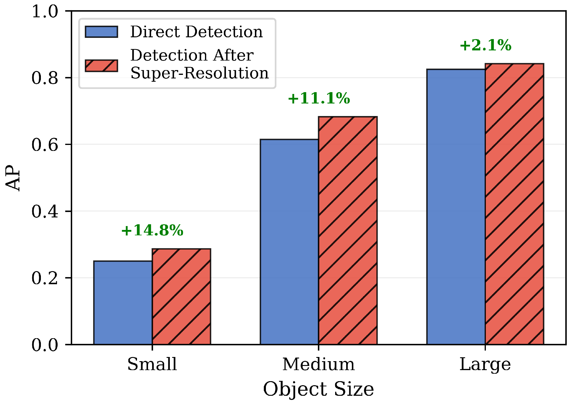
To illustrate this limitation, we conduct experiments on the COCO dataset [44], which contains objects of widely varying scales and thus exposes the sensitivity of detection to resolution. Focusing on person detection, we use YOLOv10 [45] to compare two pipelines: direct detection on original images and detection after upscaling images to 4× resolution with Real-ESRGAN [46], a super-resolution model. The results in Figure 1 show that applying super-resolution leads to only a modest 14.8% improvement. The overall accuracy for small objects remains at 0.28.

These findings highlight a fundamental challenge: the lack of sufficient visual information in small objects cannot be compensated by software-based enhancements alone. This motivates the need for a different perspective on video analytics, one that directly increases the amount of useful visual information available for small objects at the point of capture rather than attempting to recover it afterward.

3.2. Potential of PTZ Cameras for Small Object Detection

PTZ cameras offer a compelling avenue to address small object challenges by enabling dynamic adjustments to camera configurations: panning (horizontal rotation), tilting (vertical rotation), and optical zooming. Optical zoom adjusts the lens focal length to enlarge object projections on the image sensor, preserving or even enhancing spatial resolution and making subtle features more discernible. This capability can potentially boost DNN inference accuracy without relying solely on post-capture processing. Specifically, we can leverage the controllability of PTZ cameras to dynamically adjust their PTZ configurations. Within each analysis cycle, different optically-enhanced subframes are acquired by tuning these configurations, and the detection results from these enhanced subframes are subsequently fused into the reference frame to improve overall analysis accuracy. 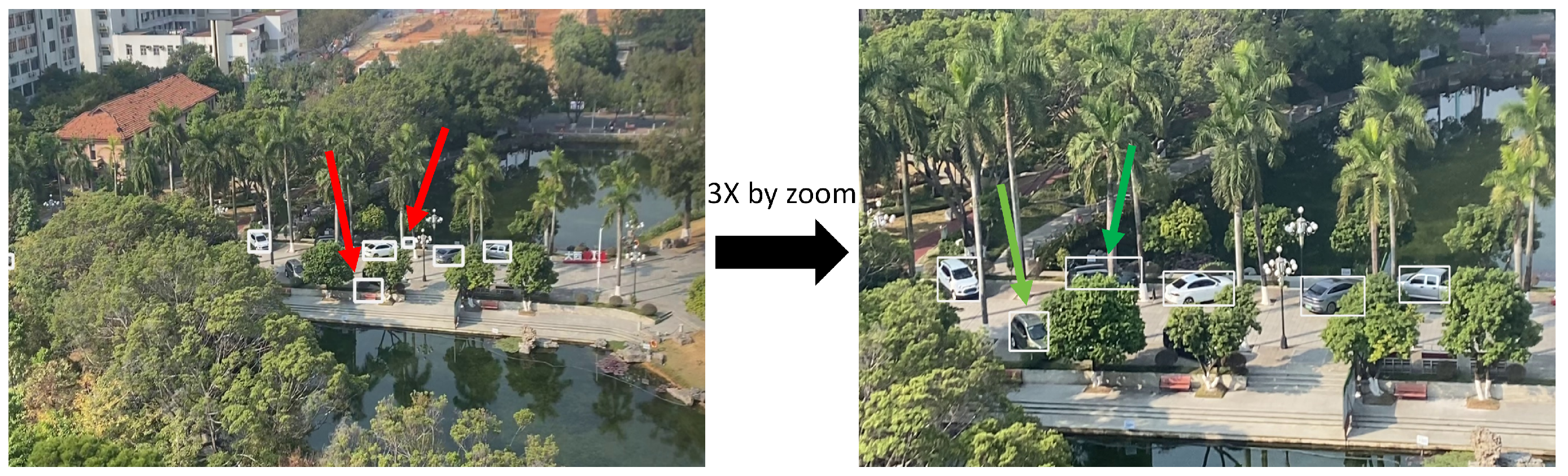Figure 2 provides example screenshots to illustrate the benefits of zoom in.

3.3. Challenges in Leveraging PTZ Cameras for Real-Time Video Analytics

While PTZ cameras hold strong potential, fully exploiting their capabilities for real-time video analytics introduces several challenges.

Mechanical Constraints. The adjustment speed of PTZ cameras is limited by their mechanical design, which restricts how frequently configurations can be adjusted in live systems.

Table 1. Representative PTZ mechanical speed specifications.

Device	Pan (°/s)	Tilt (°/s)	Zoom Time (s)
Hikvision DS-2DE2204IW/XM (Hangzhou Hikvision Digital Technology Co., Ltd., Hangzhou, China)	60	50	2 ($1\times$ →  $4\times$)
Hikvision iDS-2PT3D40IX (Hangzhou Hikvision Digital Technology Co., Ltd., Hangzhou, China)	60	50	1.7 ($1\times$ →  $4\times$)

shows representative specifications for two commercial models. For example, the Hikvision DS-2DE2204IW/XM (Hangzhou Hikvision Digital Technology Co., Ltd., Hangzhou, China) [47] can rotate only about $2°$ or zoom by approximately $0.06\times$ within a typical analysis cycle of 33 milliseconds (corresponding to 30 frames per second). When such cameras are directly integrated into conventional video analytics pipelines, only a small fraction of the possible PTZ adjustments can be applied per analysis cycle, leading to limited accuracy improvements.

Optimal configuration determination. Determining the set of configurations within an analysis window that maximizes accuracy is non-trivial. A PTZ configuration is formally represented as a triplet $(p,t,z)$, corresponding to pan, tilt, and optical zoom. Since these parameters are driven by independent motors, the transition time between two configurations is dictated by the parameter requiring the longest adjustment duration. For example, in the Hikvision DS-2DE2204IW/XM, transitioning from an initial state of $(0°,0°,1\times )$ to $(10°,10°,2\times )$ requires 0.66 s. This latency is calculated as $max(0.16\mathrm{s},0.16\mathrm{s},0.66\mathrm{s})$, where the zoom adjustment acts as the bottleneck. Because each potential configuration incurs a distinct time cost and offers a different potential accuracy gain, selecting the optimal sequence that fits within a strict time budget (analysis cycle) while yielding the highest expected accuracy constitutes a fundamental challenge.

These challenges motivate ZoomPatch, a framework that dynamically schedules PTZ configuration adjustments to improve small object detection in real-time video analytics.

4. ZoomPatch Design

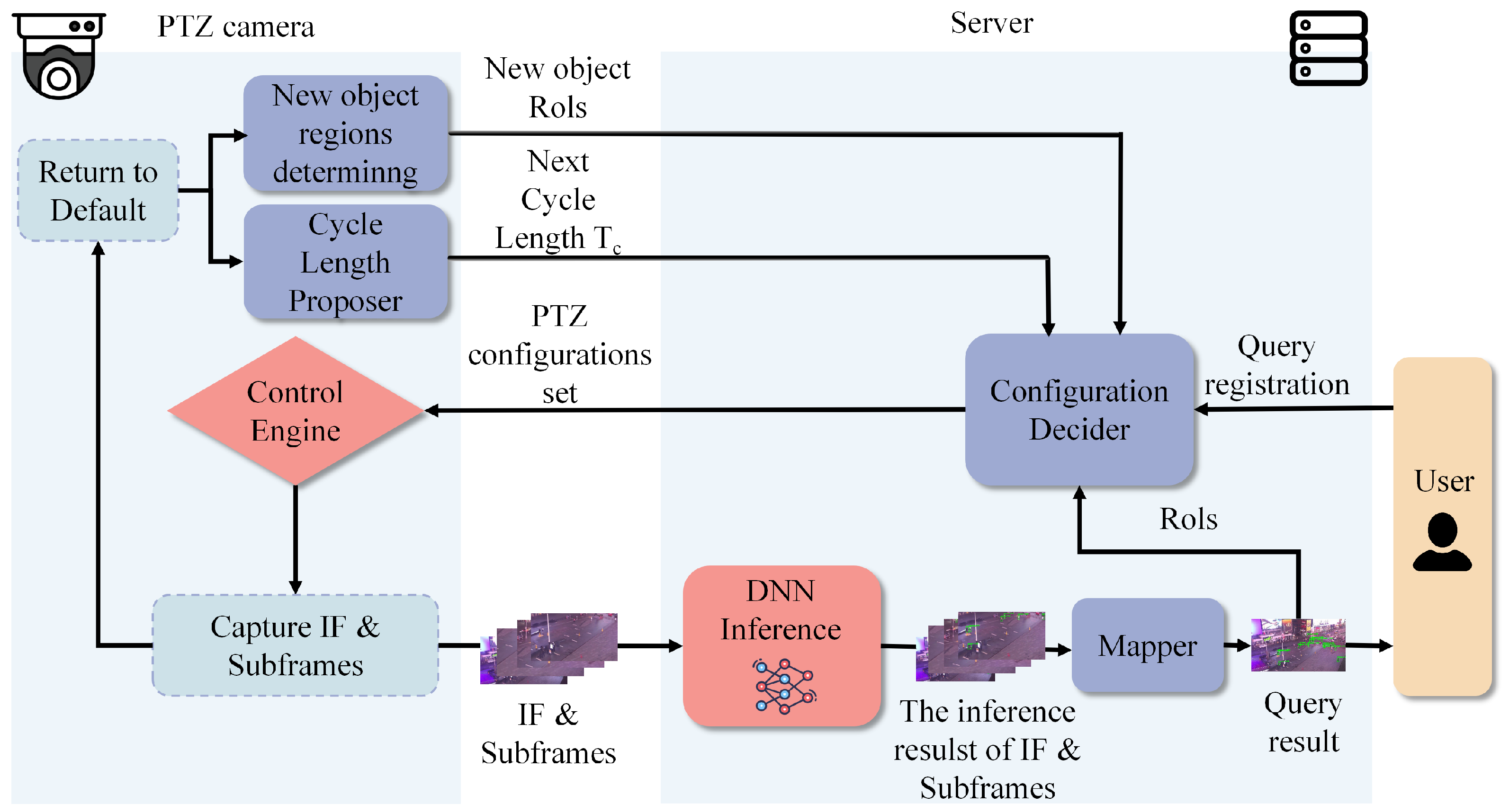
To address the mechanical constraints and optimal configuration determination challenges of PTZ cameras in video analytics, we propose ZoomPatch, an end-to-end framework incorporating a dynamic Cycle Length Proposer and a MILP-based Configuration Decider. By leveraging scene motion characteristics to dynamically extend analysis cycles and determining optimal PTZ configurations, the system maximizes analytical accuracy gains. Figure 3 shows the system overview of ZoomPatch.

4.1. Overview Workflow

The workflow of ZoomPatch begins when a user submits a video analytics query, specifying a target scene, the model to use, the object(s) of interest, and the task.

Each analytics cycle starts with the PTZ camera capturing an initial wide-field-of-view frame (IF), i.e., default configuration ($0°$, $0°$, $1\times$), for reference frame. Subsequently, using the PTZ configuration sequence computed by the Configuration Decider from the previous cycle (detailed in Section 4.3), the camera executes a series of targeted adjustments. For each configuration $(p,t,z)$, it pans, tilts, and optically zooms to focus on ROIs, capturing optically enhanced subframes that enlarge small objects for improved resolution and feature discriminability. The reference frame and subframes are compressed and streamed to the server, where the DNN performs inference and generates detections (e.g., bounding boxes, classes, and confidence scores).

Once all subframes in the cycle have been captured, the PTZ camera is reset to its default configuration. Concurrently, the Cycle Length Proposer (Section 4.2) evaluates the motion intensity within the current cycle’s video stream—primarily using sparse Lucas–Kanade optical flow on consecutive IFs—and determines the adaptive cycle length for the next window (Challenge 1). This extends the cycle for low-motion scenes to permit more subframes or shortens it for high-motion scenes to maintain tracking fidelity. Upon completion of server-side inference, the Mapper component inversely projects subframe results back to the reference frame’s coordinate system. It aggregates baseline reference frame detections with enhanced subframes outputs, resolves overlaps using non-maximum suppression, and delivers the final query results to the user.

After mapping, the server signals the camera to transmit outputs from its components: New Object Suggester, which predicts potential emerging ROIs for small objects, and the Cycle Length Proposer, which proposes the next cycle’s length based on recent object motion intensity. The server’s Configuration Decider then integrates these inputs with the current query results to solve the optimization problem, deriving the optimal PTZ sequence for the upcoming cycle (Challenge 2). This closes the loop, with the process repeating seamlessly for subsequent cycles, ensuring continuous adaptation to dynamic scenes while maximizing accuracy for small objects.

4.2. Cycle Length Proposer

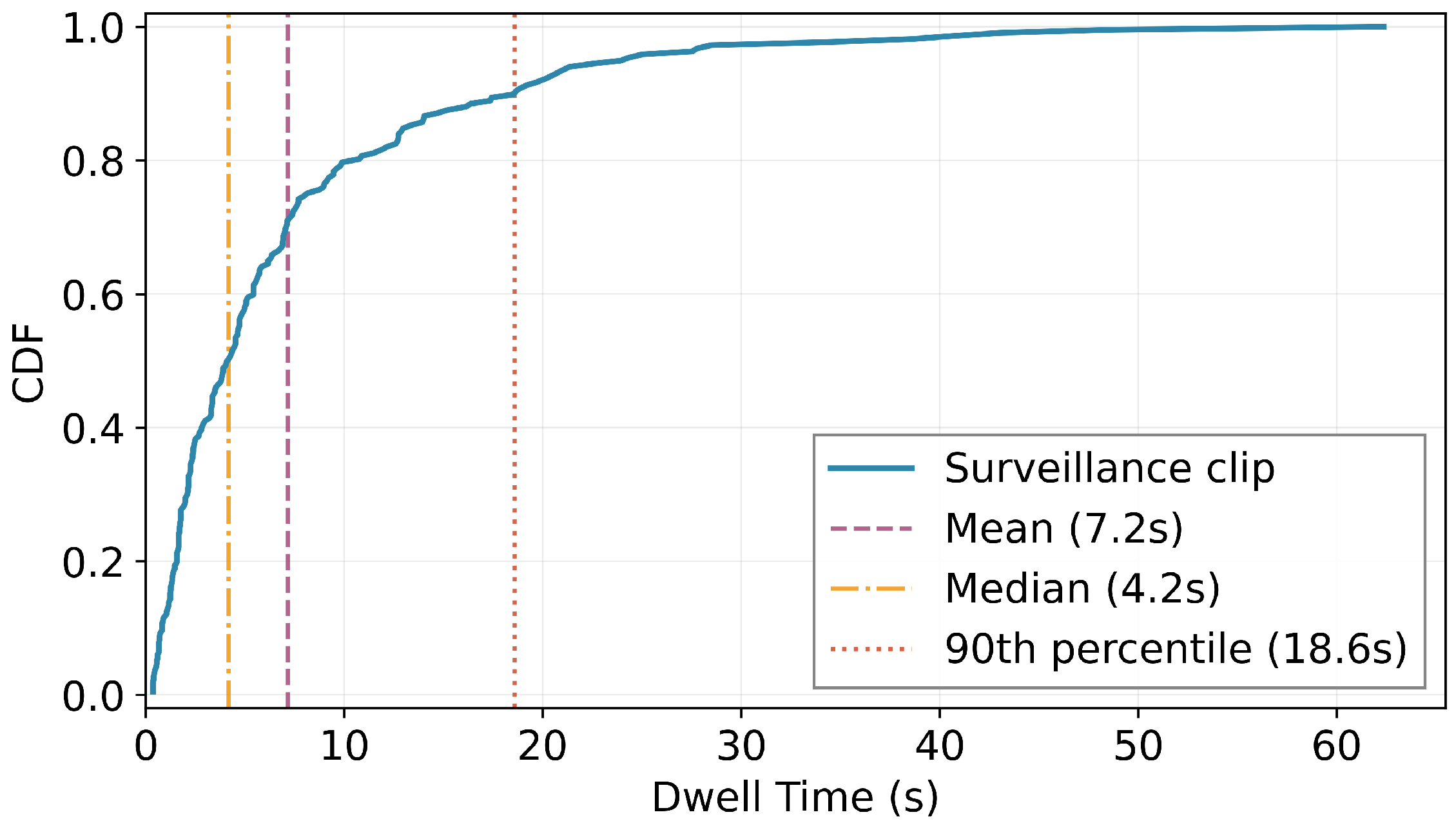
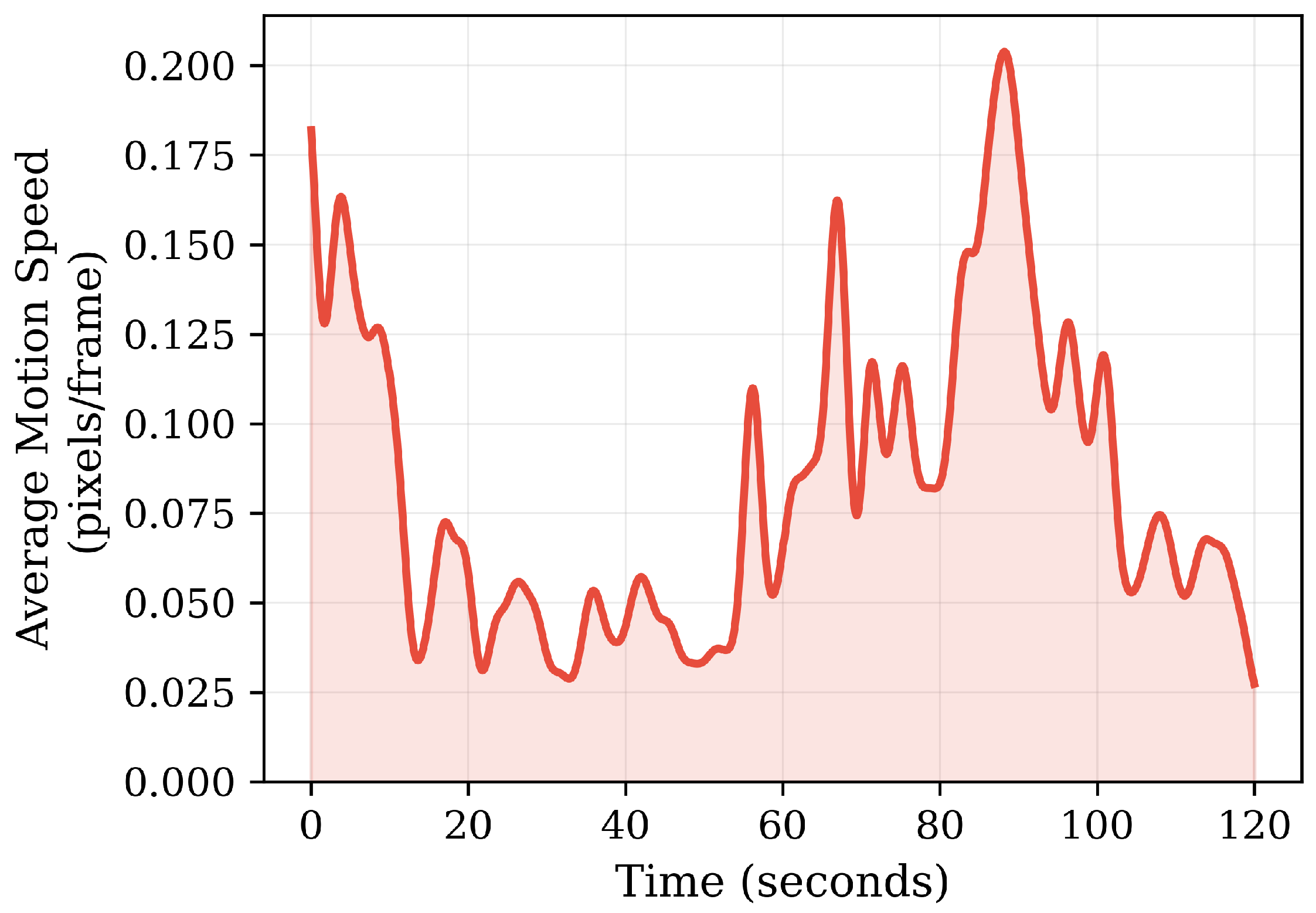
As illustrated in Figure 4, a surveillance clip has an average dwell time of 7.16 s and a median of 4.17 s for pedestrian. In other words, small object scenes exhibit a key property: objects tend to remain in view for a relatively long duration. Leveraging this property, proactively extending the analysis cycle will not lead to object omission or subsequent accuracy degradation. In addition, as illustrated in Figure 5, the speed of object motion in videos—quantified by the mean optical flow magnitude—vary dynamically over time. To adapt to these changes, ZoomPatch employs a self-adaptive analysis cycle length: longer cycles are used in low-motion scenes to allow more PTZ adjustments to capture subframes, while shorter cycles are preferred in high-motion scenarios to prevent object loss and maintain accuracy.

In summary, the Cycle Length Proposer determines the length of the analysis cycle based on the current scene’s motion intensity, measured via optical flow estimation. Specifically, it computes the motion strength using the sparse Lucas–Kanade optical flow method [48] on consecutive default settings. This yields the average displacement vector magnitude, denoted as ${\mu }_d$, which serves as a proxy for overall scene dynamics.

Formally, the cycle length $T_c$ for the next cycle is calculated as:

$$T_c=T_{min}+(T_{max}-T_{min})\times \left(1-{\displaystyle \frac{{\mu }_d}{{\mu }_{max}}}\right),$$

(1)

where $T_{min}$ represents the minimum cycle length, anchored to the minimum observed object dwell time in the target scene to guarantee minimal latency and responsiveness even under rapid motion. $T_{max}$ denotes the maximum cycle length, capped at the median object dwell time to prevent excessive delays while fully exploiting persistence in slow scenes. ${\mu }_d$ is the measured mean optical flow magnitude of IFs from the current cycle. ${\mu }_{max}$ is the maximum expected optical flow magnitude, representing high-motion thresholds.

These configurations ($T_{min}$, $T_{max}$, and ${\mu }_{max}$) are calibrated offline by analyzing a representative video segment from the deployment environment to capture characteristic motion patterns. For instance, in a typical urban pedestrian monitoring scenario, $T_{min}$ might be set to a value reflecting shorter dwell times (e.g., a few hundred milliseconds), while $T_{max}$ aligns with the median of approximately 4 s. Through this adaptive mechanism, ZoomPatch improves the accuracy of small object video analytics by enabling targeted PTZ adjustments to capture enhanced subframes, while minimizing object loss induced by these adjustments to the greatest extent possible.

4.3. Configuration Decider

The core responsibility of the Configuration Decider is to determine the optimal sequence of PTZ adjustments within the dynamic time budget $T_c$ provided by the Cycle Length Proposer. In this section, we describe the system model and formulate the PTZ scheduling problem as an optimization task.

4.3.1. System Model

Candidate Configuration and Indexing: A PTZ configuration is formally represented as a triplet $(p,t,z)$, denoting pan angle, tilt angle, and optical zoom level, respectively. We discretize the configuration space starting from the default setting $(0°,0°,1\times )$ with increments of $10°$ for pan, $5°$ for tilt, and $0.1\times$ for zoom, ensuring all generated subframes remain within the boundaries of the original field of view to maintain comprehensive scene coverage. The set of generated candidate subframe configurations is indexed by $\mathcal{S}=\{0,1,\dots ,N\}$, where 0 represents the initial depot configuration.

Accuracy Gain Model: To quantify the benefit of PTZ adjustments, let $w_{s,o}$ represent the expected inference accuracy gain obtained by covering object o with subframe s. The accuracy gain $w_{s,o}$ is defined as the improvement in detection probability achieved by enlarging the object from its original size ${\mathrm{size}}_o$ to its projected size under zoom level $z_s$:

$$w_{s,o}=\left\{\begin{array}{cc}\mathcal{P}\left(\mathcal{Z}(z_s,{\mathrm{size}}_o)\right)-\mathcal{P}\left({\mathrm{size}}_o\right),\hfill & o\mathrm{is}\mathrm{completely}\mathrm{covered}\mathrm{by}s\hfill \\ 0,\hfill & \mathrm{otherwise}\hfill \end{array}\right.$$

(2)

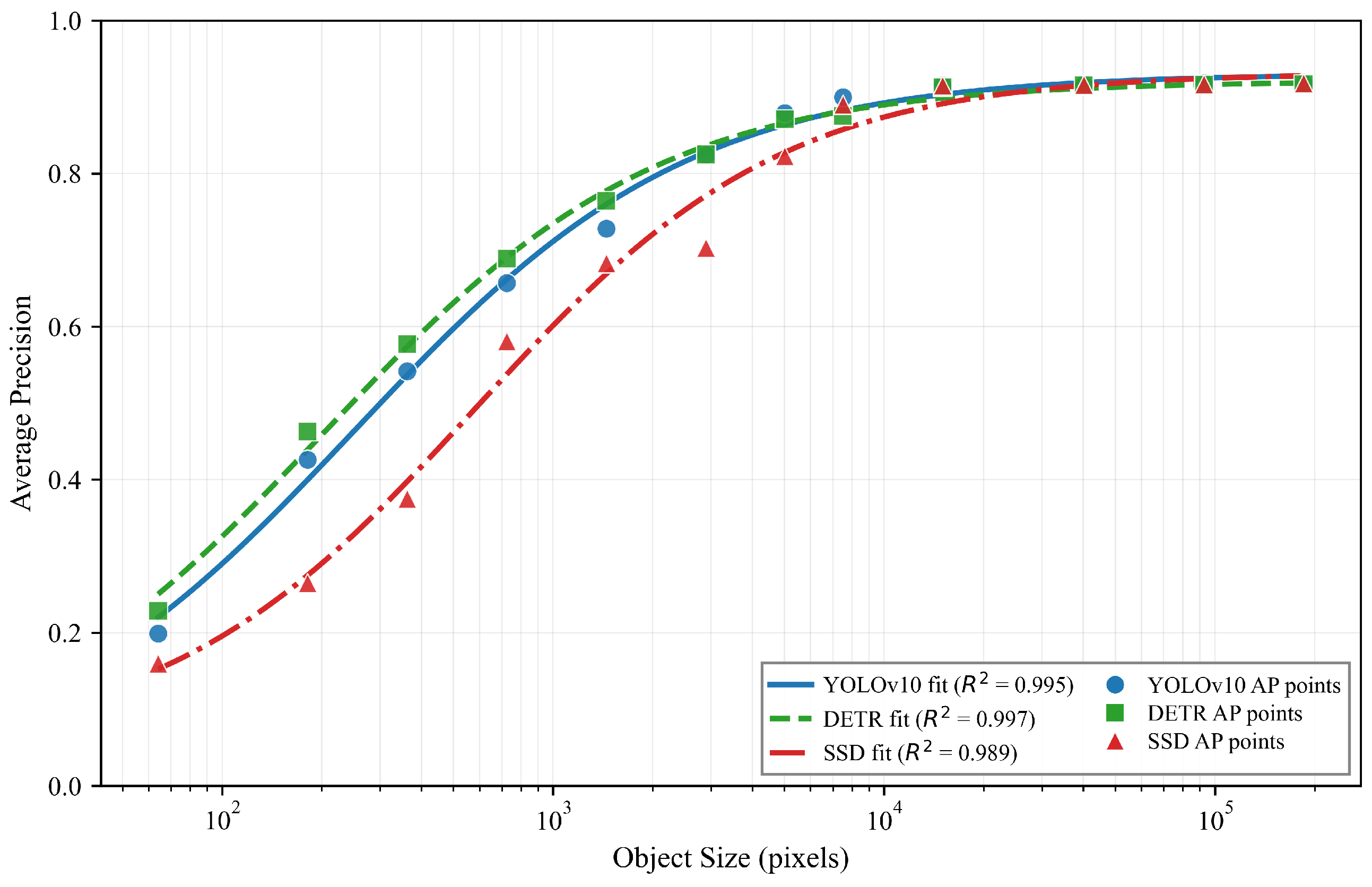
Here, $\mathcal{P}(·)$ is the detection probability function, i.e., the fitted curve shown in Figure 6 and $\mathcal{Z}(·)$ represents the enhanced object size.

To construct the empirical profiling curves shown in Figure 6, we conducted an offline evaluation using the COCO dataset. First, we categorized the ground-truth bounding boxes of objects (e.g., people) into discrete size intervals. For each interval, we calculated the average precision, which corresponds to the scattered points in Figure 6. Finally, we applied logistic regression to fit these discrete points and generate the continuous profiling curves.

PTZ Scheduling Latency: The mechanical latency $m_{i,j}$ required to transition from configuration i to j is determined by the slowest mechanical component, as PTZ operations occur simultaneously. It is modeled as:

$$m_{i,j}=max\left({\displaystyle \frac{|p_i-p_j|}{v_{pan}}},{\displaystyle \frac{|t_i-t_j|}{v_{tilt}}},{\displaystyle \frac{|z_i-z_j|}{v_{zoom}}}\right),$$

(3)

where $v_{pan}$, $v_{tilt}$ and $v_{zoom}$ are the transition camera’s speeds for the pan, tilt, and zoom dimensions. Note that $m_{i,j}$ represents a constant latency matrix pre-calculated based on the camera’s mechanical specifications prior to optimization, not a decision variable.

4.3.2. Problem Formulation

Let $\mathcal{O}$ be the set of objects and $\mathcal{S}$ be the set of candidate subframes (including the depot 0). The objective is to select a subset of subframes and a visitation order to maximize total accuracy gain without exceeding the time budget $T_c$.

We define the decision variables as follows: let $x_s\in \{0,1\}$ be a binary variable indicating if subframe s is selected; $y_{o,s}\in \{0,1\}$ is a binary variable indicating whether object o is effectively assigned to subframe s for accuracy gain accounting; and $z_{i,j}\in \{0,1\}$ is the routing variable for transitioning from subframe i to subframe j. Additionally, we introduce auxiliary variables $u_i\in [0,N]$ denote the visit order of subframe i, used for subtour elimination. The optimization problem ${\mathcal{P}}_{PTZ}$ is formulated as follows:

$$\begin{array}{cc}\hfill \max & Z=\sum _{o\in \mathcal{O}}\sum _{s\in \mathcal{S}}{w}_{s,o}·y_{o,s}\hfill \\ \hfill \mathrm{s}.\mathrm{t}.& C_1:\sum _{s\in \mathcal{S}}{y}_{o,s}\le 1,\forall o\in \mathcal{O}\hfill \\ \hfill & C_2:y_{o,s}\le x_s,\forall o\in \mathcal{O},\forall s\in \mathcal{S}\hfill \\ \hfill & C_3:\sum _{j\in \mathcal{S}}{z}_{0j}=1,\sum _{i\in \mathcal{S}}{z}_{i0}=1\hfill \\ \hfill & C_4:\sum _{j\in \mathcal{S},j\ne k}{z}_{k,j}=\sum _{i\in \mathcal{S},i\ne k}{z}_{i,k}=x_k,\forall k\in \mathcal{S}\hfill \\ \hfill & C_5:\sum _{i\in \mathcal{S}}\sum _{j\in \mathcal{S},j\ne i}{m}_{i,j}·z_{i,j}\le T_c\hfill \\ \hfill & C_6:u_i-u_j+\left|\mathcal{S}\right|·z_{i,j}\le \left|\mathcal{S}\right|-1,\forall i,j\in \mathcal{S}\setminus \left\{0\right\}\hfill \end{array}$$

(4)

Constraint $C_1$ ensures that the accuracy gain for each object is counted at most once, preventing double-counting if an object is covered by multiple selected subframes. $C_2$ enforces logical consistency, ensuring an object is covered only if the corresponding subframe is selected. $C_3$ ensures the PTZ scheduling trajectory is a closed loop starting from the initial configuration. $C_4$ maintains flow conservation for the camera path, ensuring that if a configuration is entered, it is also exited. $C_5$ guarantees that the total mechanical transition time does not exceed the dynamic budget $T_c$. Finally, $C_6$ employs the Miller-Tucker-Zemlin formulation to prevent disconnected subtours in the camera’s trajectory.

Note that the objective function is a linear summation of accuracy gains, and all constraints ($C_1$ through $C_6$) are linear inequalities or equalities. Therefore, the overall optimization problem ${\mathcal{P}}_{PTZ}$ constitutes a MILP formulation. This structure allows for efficient resolution using commercial solvers, as demonstrated in our implementation with Gurobi [49].

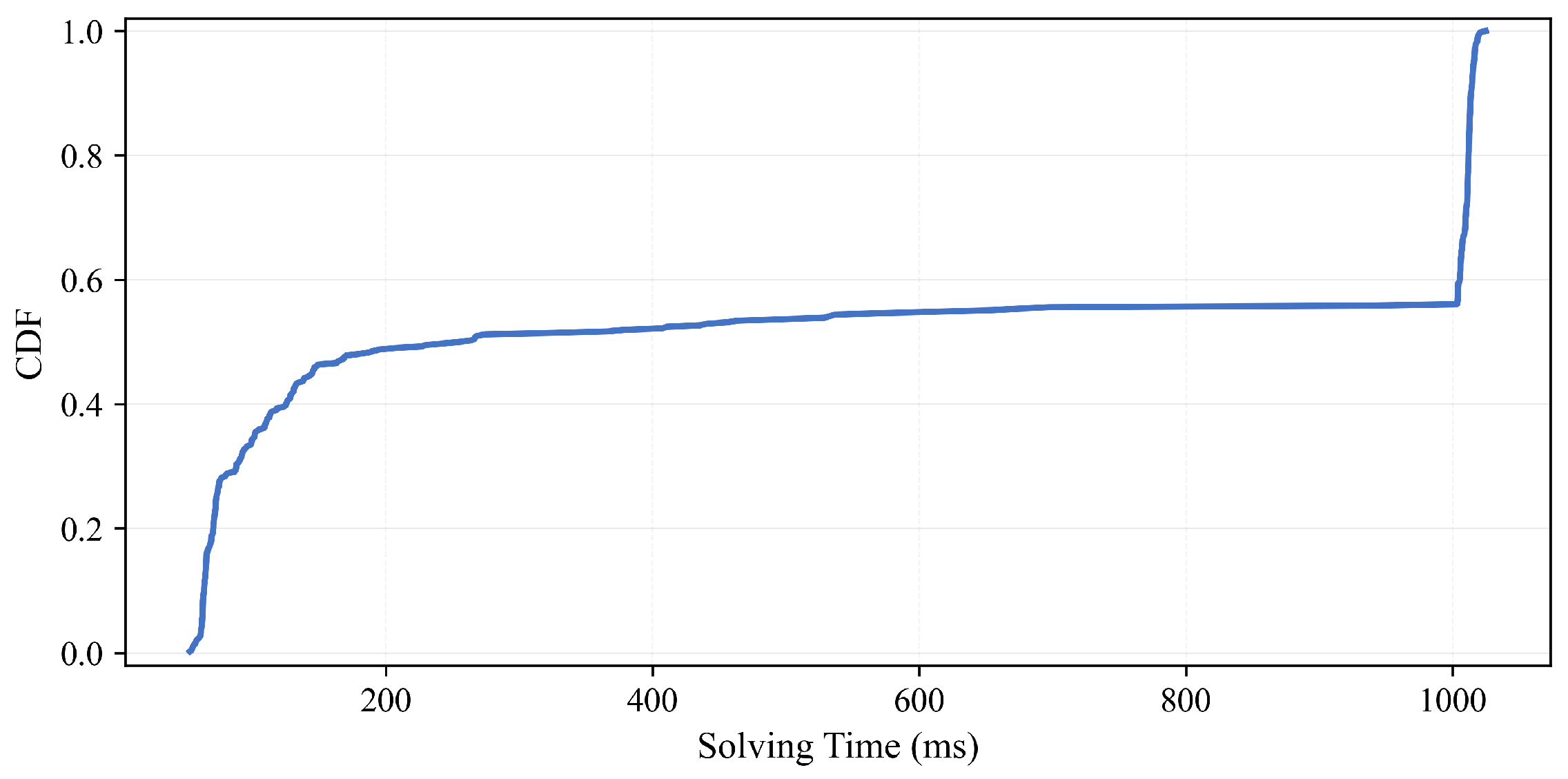
While our MILP formulation mathematically defines the optimal PTZ configuration sequence, solving it to proven optimality in highly dense scenes (e.g., when the candidate set and object set are large) can exceed the dynamic time budget $T_c$. To strictly guarantee real-time system performance, we enforce the TimeLimit (1 s) on the Gurobi solver. If the solver exhausts this time budget before proving global optimality, it leverages its branch-and-bound anytime property to immediately return the best feasible integer solution found so far. This design ensures that ZoomPatch gracefully degrades to a high-quality, near-optimal scheduling strategy under extreme computational loads, never violating the latency constraints of the real-time video analytics pipeline (see Figure 7).

4.4. New Object Suggester and Mapper

4.4.1. New Object Suggester

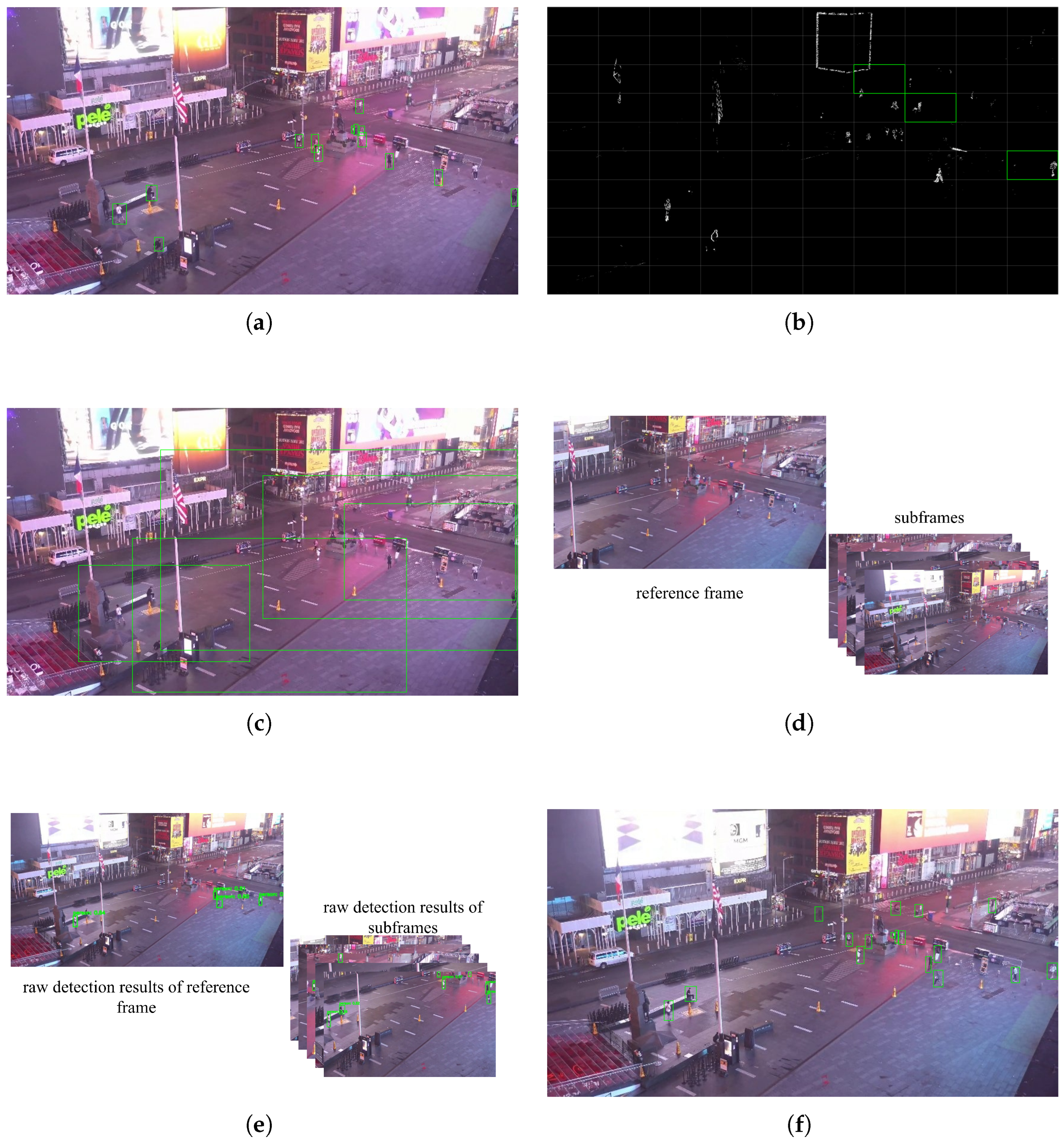
The New Object Suggester component is designed to prevent the omission of newly emerging objects of interest by identifying regions that may contain potential targets. These suggested regions are combined with the detection results from the previous query to form the updated object set $\mathcal{O}$, which serves as one of the key inputs to the Configuration Decider. The New Object Suggester operates based on a frame differencing method. After the camera has captured all subframes and returned to the initial field of view, we denote the frame captured at time t during this period as $f_t$. We first convert both $f_t$ and the previous frame $f_{t-1}$ from RGB mode to grayscale. Next, we compute the absolute pixel-wise difference between these two grayscale images to obtain the difference frame $f_{\mathrm{diff}}$. To accelerate processing, as shown in Figure 7b, we divide $f_{\mathrm{diff}}$ into multiple 16 × 16 regions. We retain only those regions where the average difference exceeds a predefined threshold T and exclude any regions that already contain known objects from the previous detections. The boundingbox of remaining retained regions are then added as new candidate objects o to the set $\mathcal{O}$.

To mitigate the impact of background motion, we assign a binary confidence value to each region. If a region x is flagged as potentially containing a new object for three consecutive cycles, but the subsequent inference results indicate no actual objects in x, it is marked as a background region with a confidence of 0. Thereafter, only regions with a confidence of 1 are considered for new object suggestions.

4.4.2. Mapper

After server-side inference is completed Figure 7e, the Mapper component inversely projects the detection results from the subframes back to the coordinate system of the reference frame.

Let the global reference frame have dimensions $W\times H$. A subframe captured at configuration $(p,t,z)$ corresponds to a Region in the reference frame with a cropped size ${\displaystyle \frac{W}{z}}\times {\displaystyle \frac{H}{z}}$. Let the camera’s horizontal and vertical Field of View be ${\theta }_H$ and ${\theta }_V$, respectively. Using the standard pinhole camera model, When the camera transitions to a new configuration $(p,t)$, the new central pixel coordinate $(c_x,c_y)$ mapped onto the global reference frame is calculated as:

$$\begin{array}{c}\hfill c_x={\displaystyle \frac{W}{2}}\left(1+{\displaystyle \frac{tan\left(p\right)}{tan({\theta }_H/2)}}\right)\end{array}$$

(5)

$$\begin{array}{c}\hfill c_y={\displaystyle \frac{H}{2}}\left(1-{\displaystyle \frac{tan\left(t\right)}{tan({\theta }_V/2)}}\right)\end{array}$$

(6)

Any pixel coordinate $(x_{sub},y_{sub})$ in the subframe can be mapped to its corresponding global coordinate $(X_{global},Y_{global})$ using the following inverse projection formulas:

$$\begin{array}{cc}\hfill X_{global}& ={\displaystyle \frac{x_{sub}}{z}}+c_x-{\displaystyle \frac{1}{2}}\times {\displaystyle \frac{H}{z}}\hfill \end{array}$$

(7)

$$\begin{array}{cc}\hfill Y_{global}& ={\displaystyle \frac{y_{sub}}{z}}+c_y-{\displaystyle \frac{1}{2}}\times {\displaystyle \frac{H}{z}}\hfill \end{array}$$

(8)

For a detected bounding box $(x_{sub},y_{sub},w_{sub},h_{sub})$ in the subframe, the mapped bounding box in the reference frame is calculated as $(X_{global},Y_{global},{\displaystyle \frac{w_{sub}}{z}},{\displaystyle \frac{h_{sub}}{z}})$.

Following the Integration of reference frame detection results with the enhanced subframes outputs, we apply non-maximum suppression to resolve any overlapping detections and deliver the final query results to the user Figure 7f.

5. Performance Evaluation

In this section, we present the implementation details of ZoomPatch, describe the experimental setup, and analyze the overall performance compared to baseline methods.

We implemented the system modules following the workflow outlined in the overview diagram. Our implementation leverages Python 3.11 and several Python libraries, including NumPy 1.24.4, OpenCV 4.9, machine learning framework Pytorch 2.0.1, and gurobipy 12.0.2.

To evaluate ZoomPatch comprehensively under repeatable and controllable conditions, we adopted a resize-based emulation approach. While field experiments provide real-world insights, they suffer from stochastic environmental factors (e.g., non-repeatable crowd motion and lighting changes) that hinder fair comparisons across different baseline. We assume a standard camera output resolution of 480p ($854\times 480$). To simulate the optical zoom mechanism, we collected high-resolution (2K) source videos. We emulate the camera capturing a frame at a specific zoom level z and orientation by cropping the corresponding ROI from the 2K source and resizing it to the target resolution ($854\times 480$) using bilinear interpolation.

This method aims to emulate the physical properties of optical zoom: a subframe with a higher zoom level utilizes more pixels from the high-fidelity source to represent the same physical area compared to the global view, thereby minimizing information loss and enhancing spatial resolution.

5.1. Evaluation Settings

Devices. We utilized a desktop PC equipped with an Intel i5-13400 CPU (Intel Corporation, Santa Clara, CA, USA) and 16 GB of RAM to act as the edge camera device. This device connects to a HUAWEI-E514RG router via a 5 GHz Wi-Fi network. The server-side processing is hosted on a workstation equipped with an AMD Ryzen 9 7950X CPU (AMD, Santa Clara, CA, USA), 128 GB of RAM, and dual NVIDIA RTX 4090 GPUs (NVIDIA Corporation, Santa Clara, CA, USA), connected to the router via Ethernet to ensure stable transmission.

Datasets. Due to the scarcity of public datasets that combine small objects, fixed viewpoints, and sufficiently high resolution to simulate optical zoom, we curated a custom dataset. We extracted 12 high-resolution (2K) video sequences from YouTube (https://www.youtube.com/watch?v=Q71sLS8h9a4, accessed on 1 February 2026); https://www.youtube.com/watch?v=rnXIjl_Rzy4, accessed on 1 February 2026). Each sequence in this dataset ranges from 5 to 10 min in duration. Furthermore, the dataset covers highly diverse environmental conditions (including sunny, cloudy, and night scenes), with an average of 10 to 30 pedestrians per frame. To establish the ground truth for these frames, we leveraged the YOLOv12-X [50] (the most capable and parameter-heavy variant of the YOLOv12 family) to generate accurate bounding box annotations across the 2K source sequences.

Tasks and Metrics. The primary goal of our proposed system is to enhance the accuracy of video analytics for small objects. To evaluate its performance, we focus on three key computer vision tasks commonly found in recent video analytics literature and real-world applications. For each task, we use specific accuracy metrics to assess effectiveness:

• Counting: This task estimates the total number of objects of interest in each individual frame. Accuracy for a given frame is measured as the percent difference between the returned and ground truth counts.
• Detection: This task localizes objects of interest by providing their precise bounding box coordinates within a frame. We use the F1 score metric, which evaluates the balance between precision and recall of the predicted bounding boxes against the ground truth boxes.
• Aggregate Counting: Unlike per-frame counting, this task counts the total number of unique objects of interest appearing throughout the duration of a scene or video segment. This is commonly used in applications such as footfall tracking. Accuracy is measured per video as the percent difference between the system’s estimated count of unique objects and the ground truth count.

Baselines. We compare ZoomPatch against several baseline methods to highlight its advantages in small object video analytics. These include: (i) fixed-perspective analysis (Direct). A standard pipeline where inference is performed directly on the global wide-angle frames without PTZ adjustments. (ii) Super-resolution enhancement (SR). A software-enhanced pipeline that applies a super-resolution model (Real-ESRGAN) to frames before inference. (iii) greedy-based subframe selection (Greedy). A PTZ configuration determine strategy that greedily selects the subframe with the highest density of small objects within the remaining time budget, but lacks the global optimization of ZoomPatch.

Models. To demonstrate the generalizability of our framework, we evaluate performance across three distinct and popular object detection architectures: SSD [51], YOLOv10 [45], and DETR [52].

5.2. Overall Results

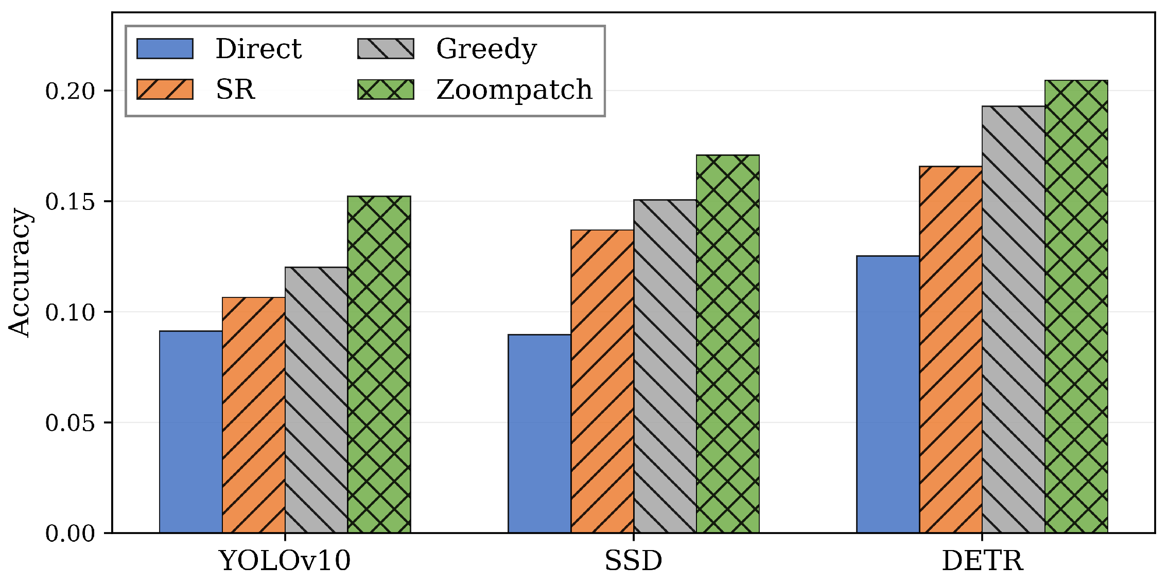
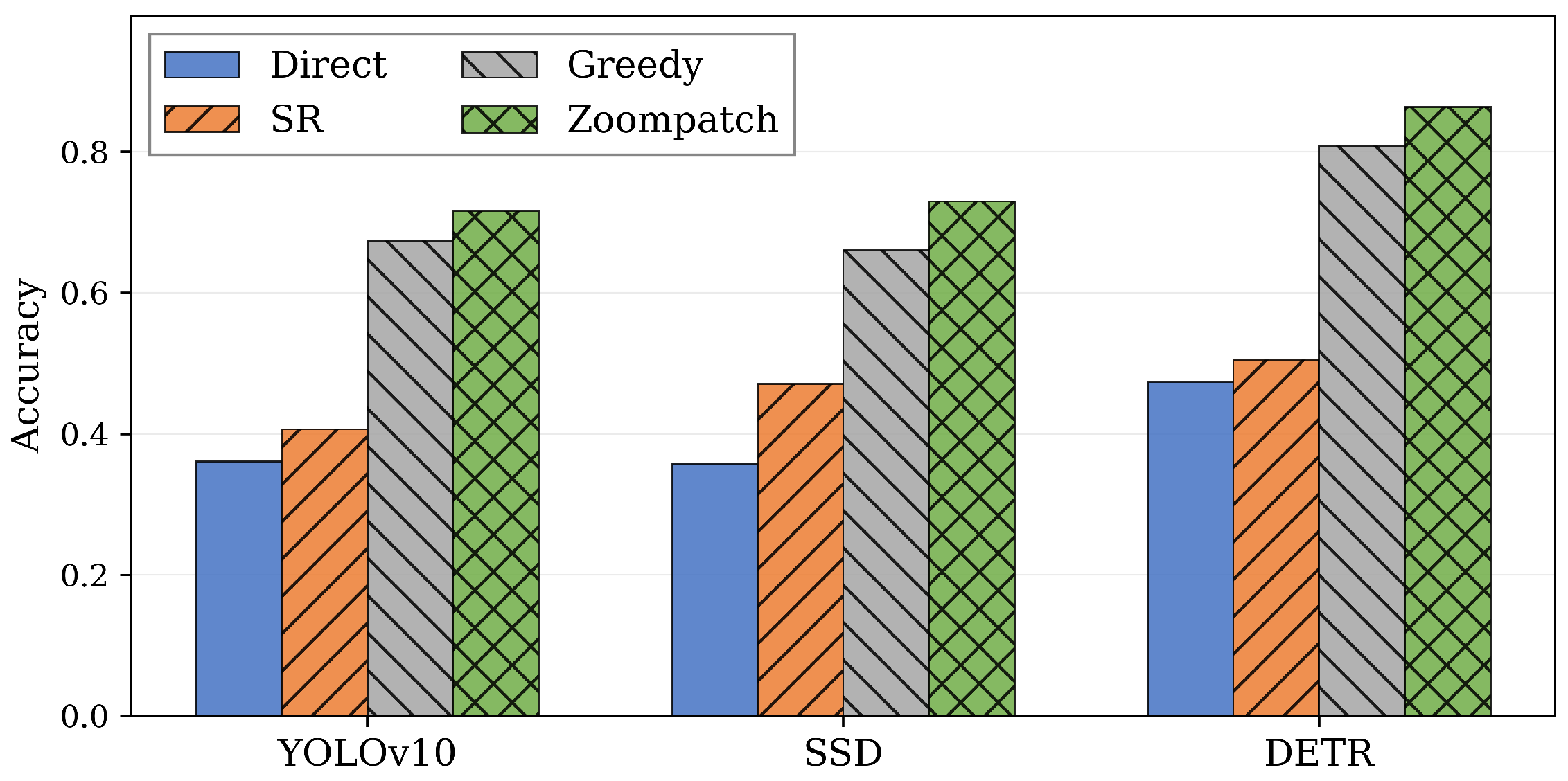
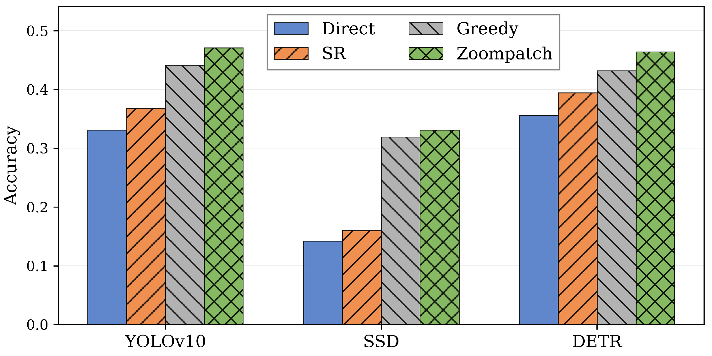
Main Performance Comparison. As illustrated in Figure 8, Figure 9 and Figure 10, ZoomPatch consistently outperforms all baseline methods in various detection tasks. Across these tasks, ZoomPatch outperforms Direct by 30–133%, SR by 18–107%, and Greedy by 4–27%. These improvements stem primarily from ZoomPatch’s optimized PTZ scheduling and optical zooming, which capture fine-grained details of small objects that SR fails to reconstruct due to information loss, and which Greedy strategies fail to capture due to inefficient time budgeting. Furthermore, as observed in the counting results (Figure 8), the performance gap between ZoomPatch and Greedy is less pronounced for DETR than for YOLOv10. Because Greedy focuses primarily on high-density regions and ignores scattered objects in the periphery, YOLOv10 suffers heavily. In contrast, DETR inherently possesses a stronger baseline capability to detect low-resolution objects (as evidenced by its higher accuracy in the Direct method), which partially mitigates the penalties of Greedy’s suboptimal zoom scheduling.

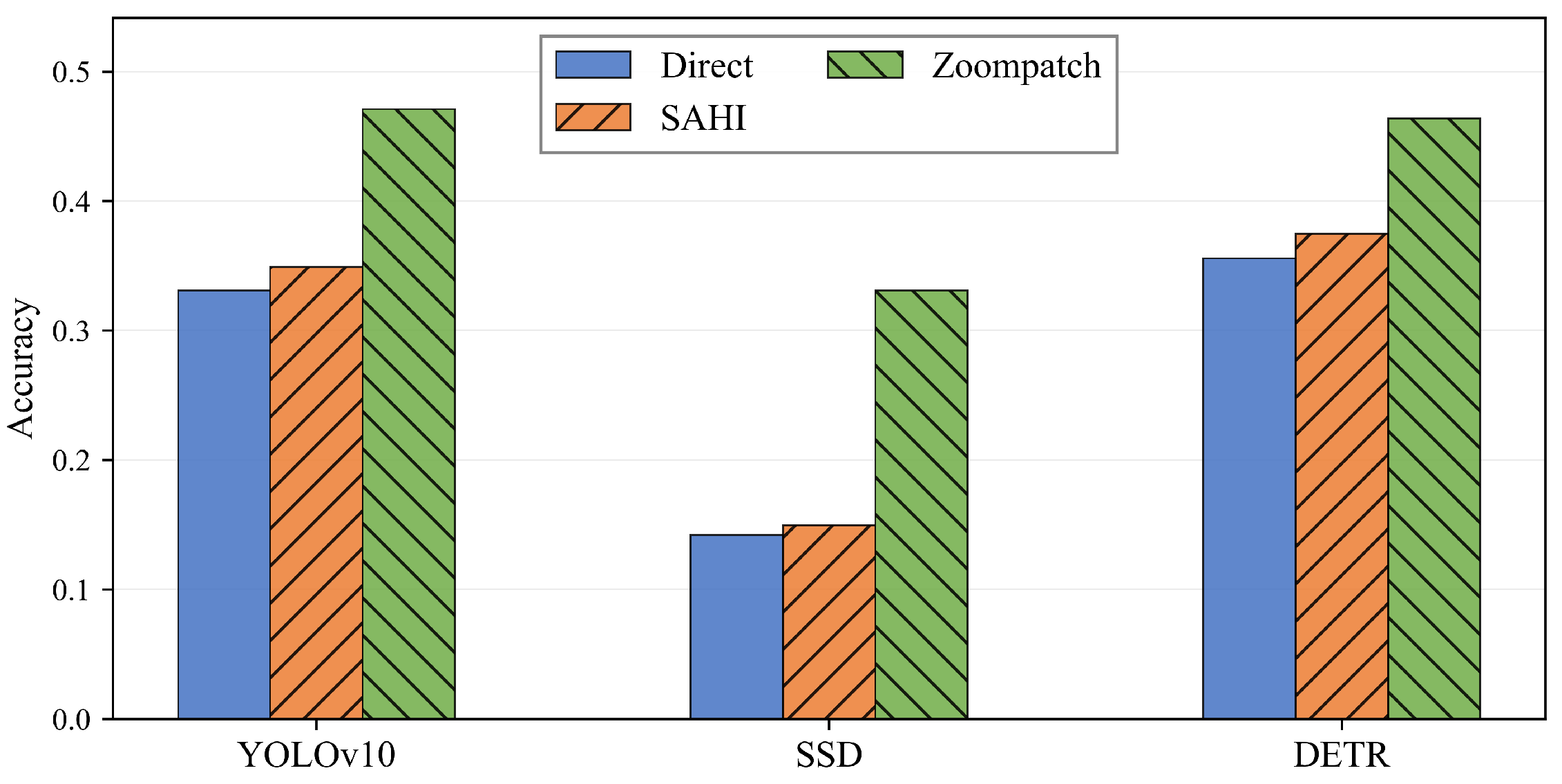
Comparison with Tile-based Detection. Tile-based detection represents a critical class of techniques for small object detection. To further demonstrate the necessity of ZoomPatch, we compared ZoomPatch against Slicing Aided Hyper Inference (SAHI), a highly representative method in this category. As shown in Figure 11, ZoomPatch significantly outperforms SAHI across all evaluated models. Specifically, compared to SAHI, ZoomPatch improves accuracy by approximately 34% (0.35 to 0.47) on YOLOv10, 120% (0.15 to 0.33) on SSD, and 21% (0.38 to 0.46) on DETR. Tile-based detection primarily excels at preventing detail loss when slicing large, high-resolution images (e.g., 4K or 2K) into smaller patches to fit standard CNN input dimensions (e.g., $640\times 640$). However, these methods inevitably fall short when the initial global view lacks sufficient spatial resolution.

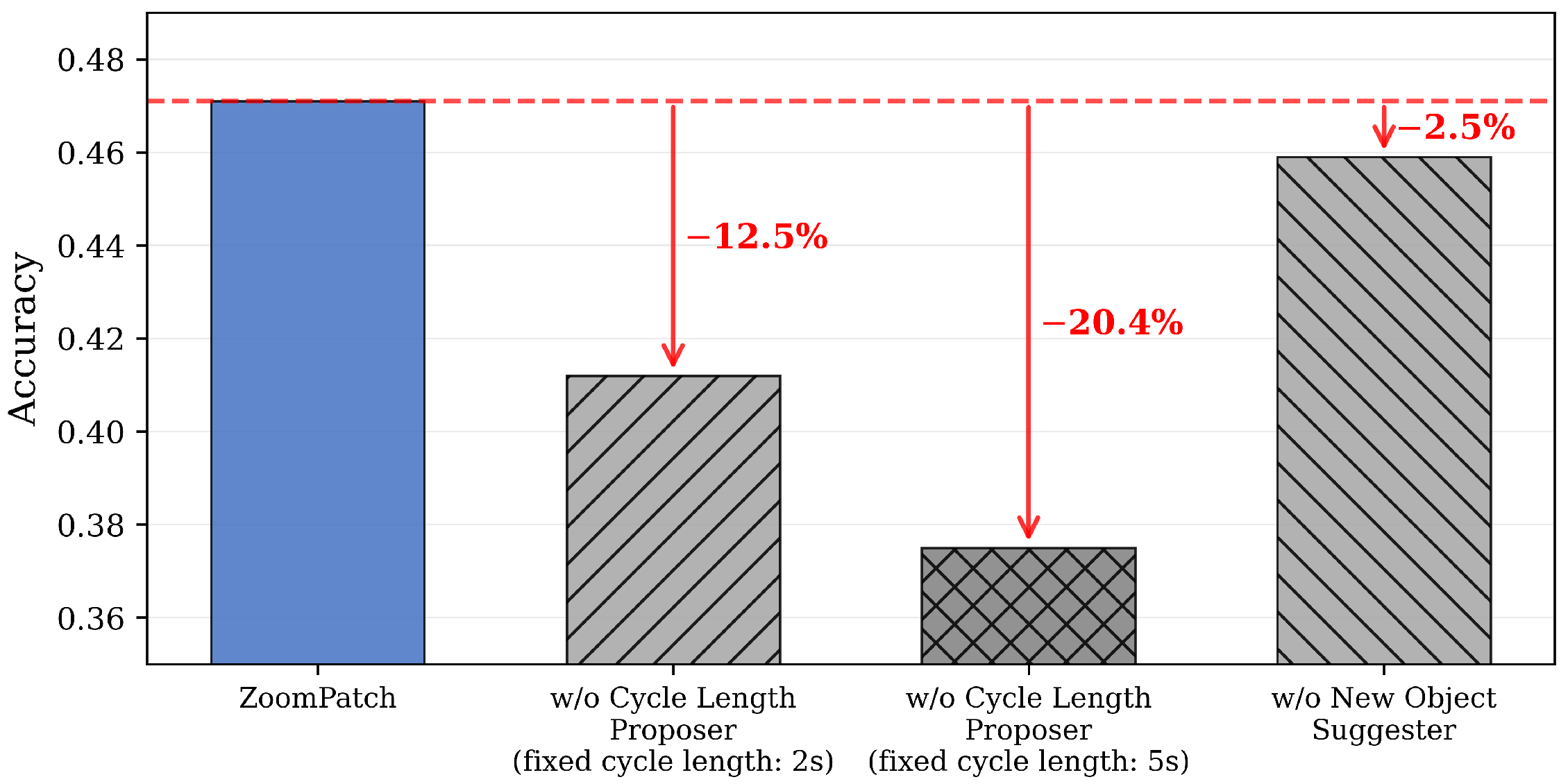
Ablation Study. We deconstruct ZoomPatch to quantify the contribution of its core modules (Figure 12). To confirm that the advantage comes from dynamic adaptability rather than simply increased analysis time, we tested fixed cycle lengths. A short fixed cycle (2 s) drops accuracy by 12.5% due to insufficient time for PTZ adjustments. Conversely, a longer fixed cycle (5 s) worsens the accuracy drop to 20.4% because fast moving objects are lost during the extended window. This proves that CLP’s dynamic time budgeting is essential. Finally, removing the New Object Suggester causes a 2.5% drop, validating its role in capturing emerging targets.

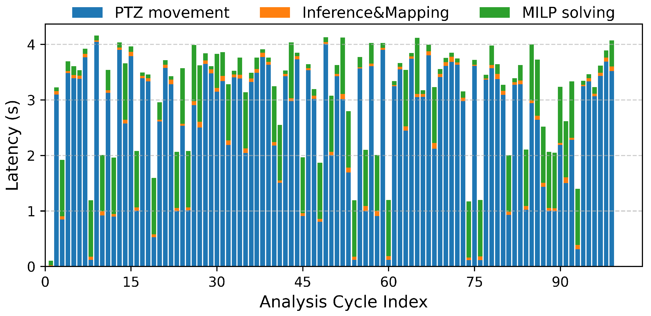
End-to-end Latency. To evaluate the real-time performance of ZoomPatch, we evaluated the end-to-end latency per analysis cycle (Figure 13). The total latency ranges from 1.0 s to 4.2 s dominated by mechanical PTZ movement. However, we respectfully clarify that the “real-time” definition in video analytics is highly context-dependent, for example, while a 1–4 s delay would be unsuitable for tracking speeding cars on a highway, it is a highly effective and fully functional “real-time” response for retail analytics and pedestrian monitoring.

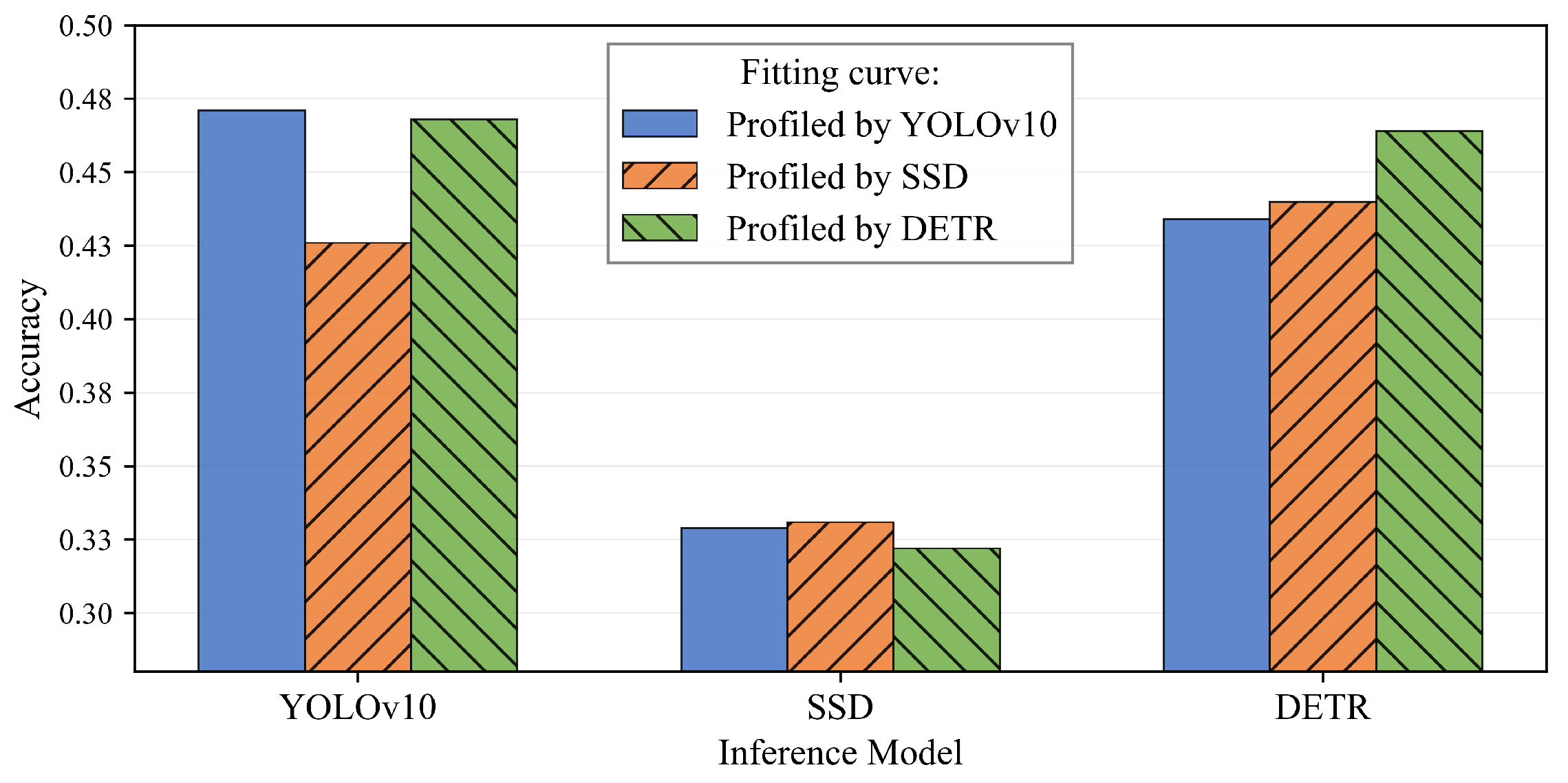
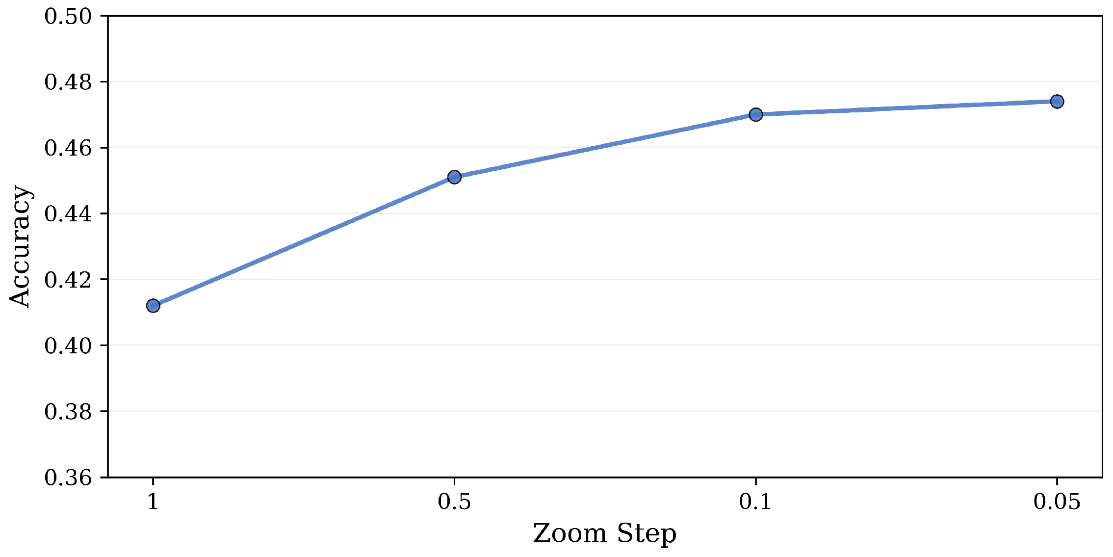
Impact of Parameter Settings. We further evaluate the sensitivity of ZoomPatch to configuration parameters. First, regarding accuracy gain model specificity, Figure 14 reveals that performance is highly sensitive to the alignment between the gain model and the inference model. Applying mismatched gain curves leads to suboptimal scheduling, underscoring the necessity of model-specific offline profiling. Second, regarding zoom search granularity, we observe that coarse step size 1 significantly degradse precision by missing optimal fields of view (Figure 15). We empirically identify a step size of 0.1 as the optimal trade-off, balancing high detection precision with low search space complexity.

Additionally, we evaluated the Gurobi solver’s execution time when set Gurobi TimeLimit to 1 s. As depicted in the CDF (Figure 16), the system operates highly efficiently in a significant portion of the scenarios: over 50% of the cycles are solved to proven global optimality in under 200 ms. However, a sharp vertical jump occurs at the 1000 ms mark, indicating that approximately 45% of the cycles trigger our enforced TimeLimit. The strict 1-s TimeLimit effectively bounds the computational overhead, ensuring the real-time feasibility of the configuration decider.

6. Conclusions

This paper introduces ZoomPatch, a real-time framework that exploits PTZ-camera zoom and rotation to boost small object detection. ZoomPatch dynamically acquires optically enhanced subframes and inversely maps their inference results back to the original frame to improve detection accuracy for small objects, addressing the limitations of passive fixed-viewpoint cameras. The key to ZoomPatch is a motion-adaptive Cycle Length Proposer that optimizes time budgets based on scene dynamics, coupled with an MILP-based Configuration Decider that selects the optimal PTZ trajectory under mechanical constraints. Extensive evaluations demonstrate that ZoomPatch consistently outperforms baseline methods. Across diverse workloads, ZoomPatch improves accuracy by 4–133%.