


Abstract
The study concerns the Duffing oscillator (Duffing equation) with softening stiffness. Using numerical simulations, the upper and lower limits of the unstable region for damping equal to 0 were identified, and analytic formulas describing them were developed. The analysis shows that the developed formulas are effective for all combinations of stiffness coefficient values that were tested. The curve of the upper limit of the unstable region is a jump-down curve, and in the theory of nonlinear systems, this curve for damping equal to zero is identified as a backbone curve (the curve of natural frequency of a system). However, the classical backbone curve calculated via a formula that is commonly known and used differs visibly from that actually obtained via numerical simulations of the upper boundary of the unstable region at large amplitudes. It could therefore be concluded that the backbone curve is not equal to the upper boundary of the unstable solution region. Moreover, the paper shows that the use of the scale relative to a critical oscillation amplitude leads to the conclusion that for damping equal to 0, systems with different parameters have the same instability regions in dimensionless space.
1. Introduction
The Duffing oscillator (Duffing equation) is a nonlinear second-order differential equation that was formulated in 1918 [1] and is used most often to model a variety of nonlinear dynamical systems. Often, depending on the issue being analyzed, the parameters of the Duffing equation are modified, and the equation is then usually referred to as a Duffing-type equation. In several cases, the modified equation is given an independent name, for example, the Duffing–Van der Pol oscillator or Helmholtz–Duffing oscillator.
The popularity of the Duffing equation (DE) and its multitude of applications have remained unchanged for years. Applications of the DE can be found not only in applied mathematics, physics, mechanics, engineering, robotics and control systems but also in optics, analytical chemistry and even social science. For example, the Duffing-Van der Pol oscillator has been applied to study the cracking-healing cycle of an asphalt mixture [2]. A two-stage Duffing equation-based oscillator and stochastic resonance have been used for mechanical fault diagnosis [3]. One study [4] focused on the energy harvesting of monostable Duffing oscillators with piezoelectric coupling under white noise excitation. The authors of another study [5] proposed strong steady-state mechanical squeezing via the joint effect between DE nonlinearity and two driving tones in an optomechanical system. A Duffing control approach has also been used to control a single risk factor in complex social–technical systems [6]. Nevertheless, the most common field in which the DE is used is mechanics, in which it is considered a mathematical model of the motion of a single degree-of-freedom system, with linear or nonlinear damping and nonlinear stiffness.
In addition to the applications mentioned above, many studies have applied the clear Duffing equation (simple or coupled) or Duffing-type equations directly [7,8,9,10,11,12]. The reason is that an exact symbolic solution to the DE does not exist. Obviously, an approximate solution can be obtained. To achieve this goal, the following analytical methods are most often used: the harmonic balance method [13,14], the iteration method [15], the perturbation or homotopy perturbation method [16,17,18], the continuation method [19] and the method of multiple scales [20]. However, when an analytical approach is used, various assumptions and simplifications should be introduced. Most often, the values of the equation parameters are constant, the damping is assumed to be close to zero, and/or the number of parameters is reduced (by transforming the equation). Notably, the derived equations refer to a steady-state solution and disregard the process of achieving it, and they very often yield a steady-state solution even in area where the equations are unstable.
Currently, with high-power computers, a numerical approach can also be used to find an approximate solution of the DE [21,22]. Importantly, there is no need to create specialized software, and one of the many available computer algebra systems (CASs) can just be used. A single numerical simulation provides results only for a specific case of the explored equation (selected equation parameters). To develop a generalized solution, simulations that involve a large set of values of equation parameters are necessary. This often makes the numerical approach very time-consuming. However, notably, in the case of dynamic systems, the results of numerical simulations are more credible than the results of calculations with equations derived via analytical methods. Therefore, the results of numerical simulations can be used to verify equations derived via analytical methods.
The last possible approach for finding an approximate solution of the DE is to perform experiments. Experiments provide results at the highest level of reality, but more importantly, experiments provide credibility to the mathematical models used to describe a given phenomenon. Unfortunately, experiments have more disadvantages than numerical approaches. The primary disadvantages are the need for an experimental station and high time and monetary costs, which often limit the use of this approach. Nevertheless, despite their disadvantages, experiments are sometimes carried out [23,24,25]. The data obtained from experiments are highly valuable and can be used similarly to the results of numerical simulations.
The Duffing oscillator in its clear form has a linear and constant damping value, a stiffness described by a cubic polynomial and simple harmonic excitation with a constant value. However, for most physical phenomena that can be described by the DE, the damping is nonlinear and varies with the vibration amplitude, and the stiffness is more complex than can be described by a cubic polynomial. Moreover, the excitation is usually not harmonic, and its value varies over time, with the possibility of external disturbances. In such cases, only experimental or numerical approaches (in which the equation parameters can be changed during the simulation) can be helpful.
This paper refers to studies on the unstable region of the standard Duffing equation with softening stiffness [26,27] and is aimed at developing analytical formulas for determining the lower and upper limits of the unstable region for damping equal to zero.
The data obtained during the research and used in the paper are available via the Mendeley Data database (https://data.mendeley.com/datasets/53v7m3xd44/1, accessed on 29 September 2025) and can be used to derive new and verify existing analytical solutions for the standard DE. Each figure included in this study to present the results of numerical simulations carried out during the research is accompanied by the name of the file that contains the data used to prepare it. Notably, the attached files contain much more data than presented in the paper (not only for damping equal to 0), and they are adequately described.
2. Duffing Equation Explored in This Research
The Duffing equation (oscillator) in its standard form, with external excitation, can be written as
where δ is the damping coefficient, α and β are coefficients that control the linear and nonlinear parts of the stiffness (α and β are also called the restoring moment coefficients), ξ is the coefficient of excitation, ω represents the oscillation angular frequency, and t represents the time. For α > 0 and β < 0, the system stiffness is softening, whereas for α > 0 and β > 0, the stiffness is hardening.
The nonlinearity of the Duffing equation is derived directly from the nonlinearity of the stiffness term (αx + βx3) and is characterized by the following coefficient:
The coefficient ε is commonly used, but it is an ambiguous parameter because we can obtain the same value of ε with different combinations of α and β (Table 1). For DE (1) with softening stiffness, the key parameter is the coefficient of the linear term α, whereas the coefficient of the nonlinear term β only determines the value of the critical amplitude Ycr (the maximum possible amplitude of oscillations) [26,27]:
Table 1.
Coefficients of the Duffing equation (softening system) considered in the study.
In the case of the hardening system, the critical amplitude does not exist.
In this research, DE (1) is analyzed, but numerical simulations are carried out for the following slightly modified equation:
The only modification in Equation (4) is the use of the time-dependent excitation coefficient ξ. This is related to the procedure for determining the lower and upper boundaries of the unstable region of the DE, which are the curves where jump-up and jump-down (bifurcations) occur.
The natural frequency of a dynamic system described by Equations (1) and (4) depend on oscillation amplitude. For the full amplitude range, it is described by the backbone curve. However, for amplitude equal to 0 it can be determined using a simple equation:
3. Numerical Simulations
Numerical simulations of DE (4) were performed for four combinations (4 cases) of coefficients α and β, all of which yielded a softening stiffness (Table 1). For the first two cases, the values of the nonlinearity coefficient ε are identical, whereas for the last two cases, they strongly differ.
Numerical simulations were carried out with the Wolfram Mathematica (CAS) computer algebra system using the Runge–Kutta method with the same initial conditions ().
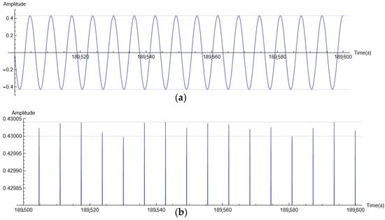
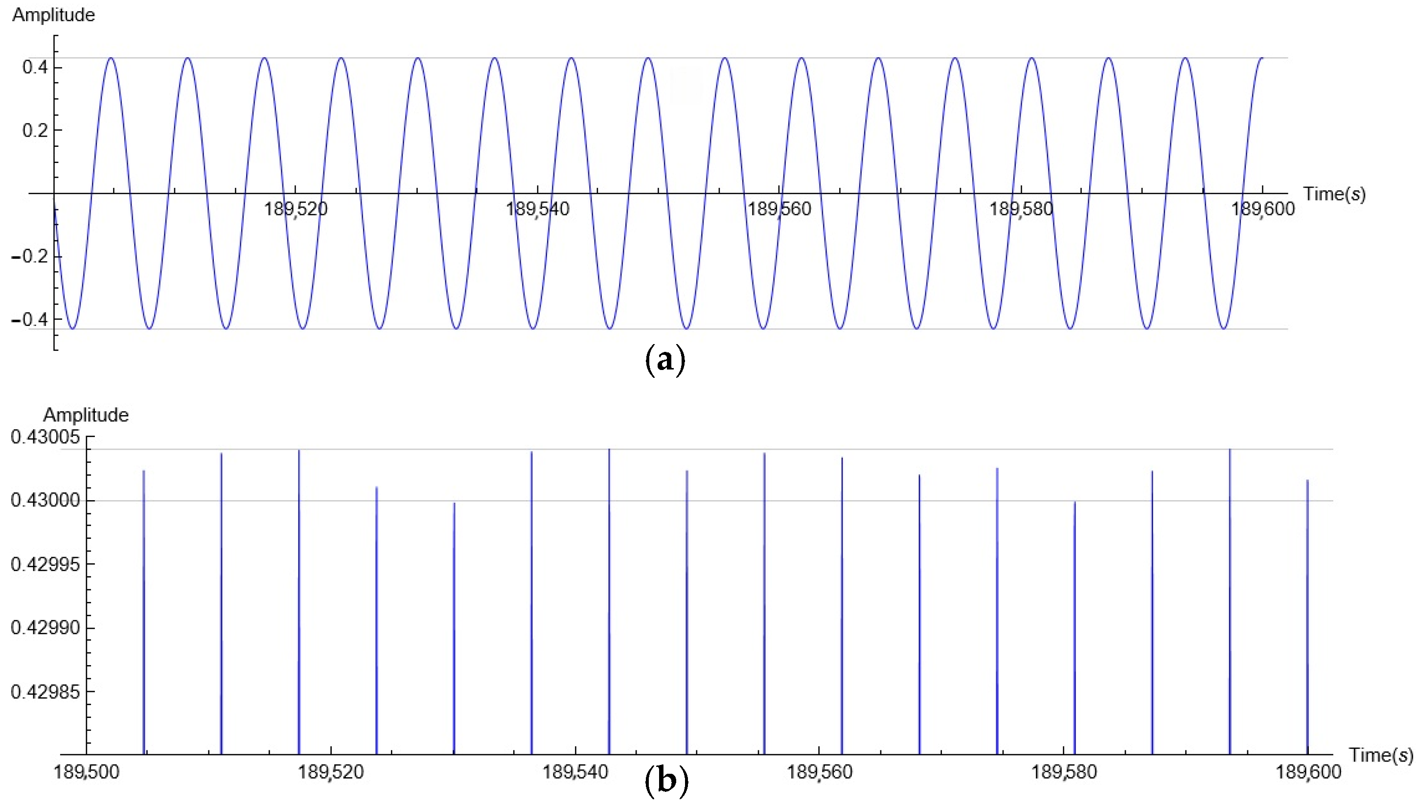
The result of each simulation should have been oscillations with a constant amplitude (steady state, SS). However, for many cases, the results of the simulations carried out with Equation (4) were not fully stable. The results of the simulation shown at the full scale (Figure 1a) indicate that the SS was reached. However, as shown in the magnified view (Figure 1b), the value of the amplitude clearly fluctuated even after 180,000 s of simulation, whereas a relatively stable result was achieved after 22,000 s. This issue was most noticeable for frequencies close to the origin point of the unstable region and for smaller values of damping. Even though the fluctuations in the amplitude were small (for the case in Figure 1, they did not exceed 0.000039), checking whether the oscillations were stable was difficult. Therefore, the simulation results were tested at 4 sections, each 800 s long, where the maximum value of the amplitude for each section was selected. The intervals between test sections were 20,000 s, 10,000 s and 10,000 s, respectively.
Figure 1.
Oscillation amplitude time history for DE (1) with η = 0.0003, α = 1.0000, β = −0.045, ω = 0.99, and excitation coefficient ξ = 0.00588; (a) full scale view; (b) magnified view.
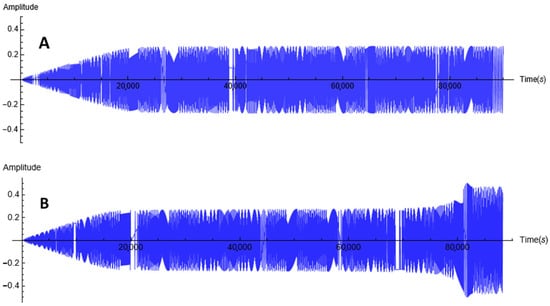
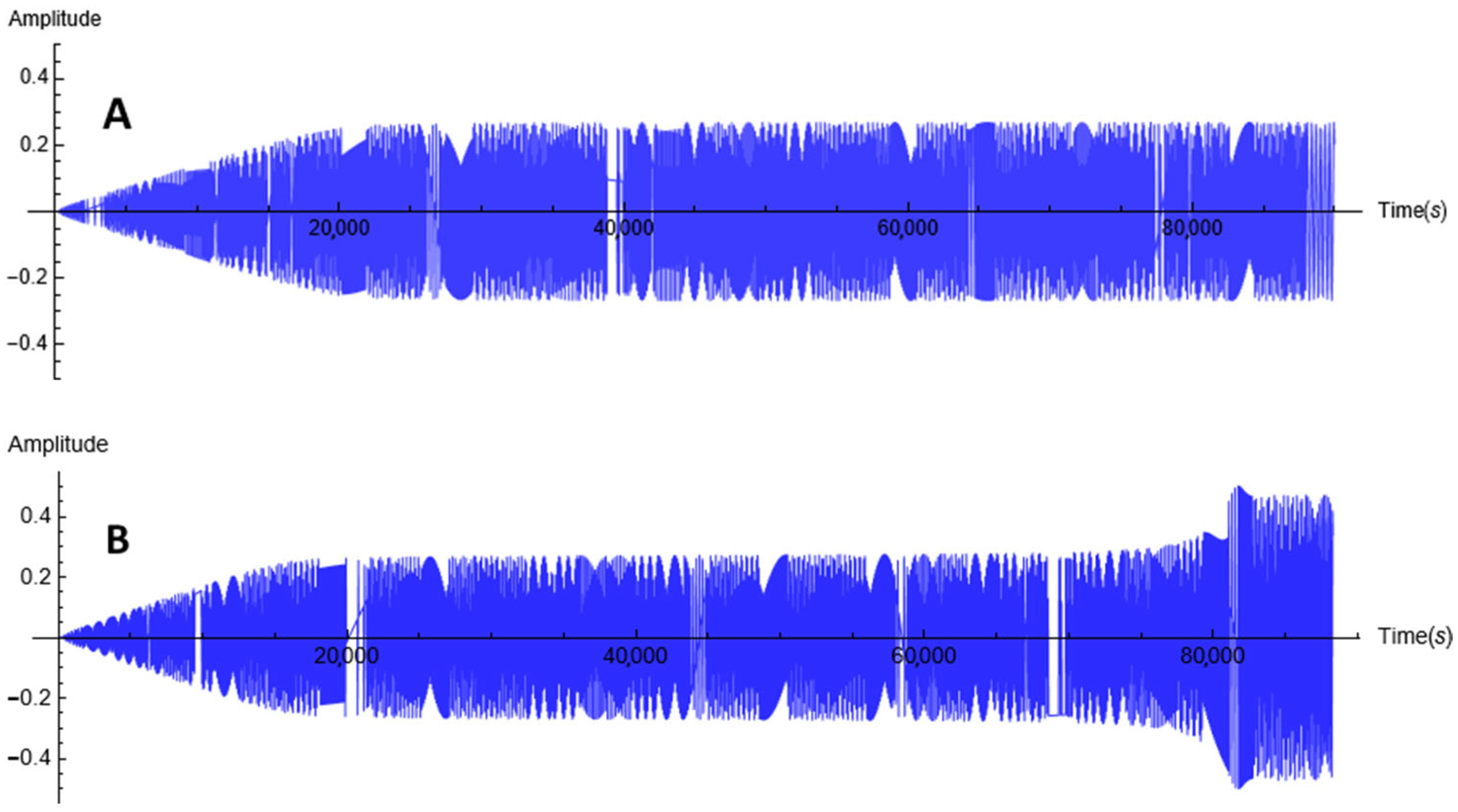
Regardless, to check the stability of the solution, the duration of most simulations was 90,000 s, and in some cases, it was extended to 190,000 s. Such a long simulation time was necessary because for oscillations with an amplitude close to the boundary of the unstable region (at the bifurcation line), the amplitude jump can be significantly delayed. In Figure 2A, the oscillation amplitude appears constant, but in fact, its value slowly but continuously increased (20,000 s: 0.244923; 38,000 s: 0.259656; 68,000 s: 0.260562; and 88,000 s: 0.260607). For this case, to observe the jump, the simulation time had to be significantly extended. In Figure 2B, to show an earlier but still delayed jump, the excitation coefficient was increased slightly. For the discussed case, the last stable amplitude, below the jump-up, was obtained for the excitation coefficient ξ = 0.0010940, and it had a value of 0.256325.
Figure 2.
Amplitude time histories for DE (1) with η = 0.001, α = 1.000, β = −0.045 and constant values of the excitation coefficient ξ = 0.0010951 (A) and ξ = 0.0010958 (B) for frequency ω = 0.997 rad/s.
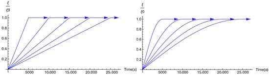
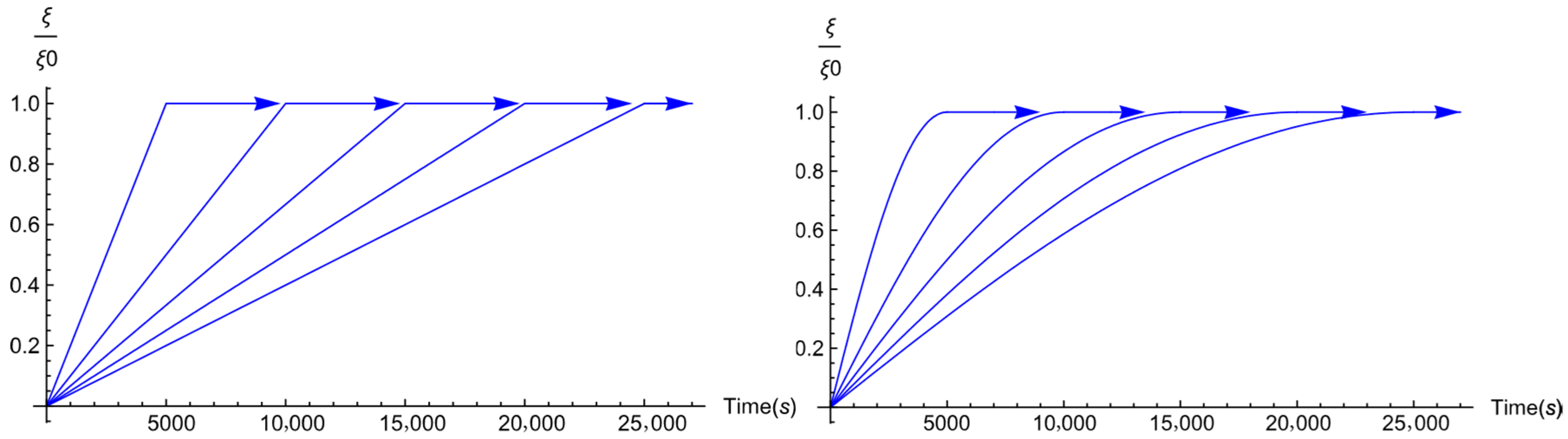
The instantaneous state of a dynamical system can be very sensitive to changes in the excitation value and frequency. Since each simulation was carried out for a constant frequency, this issue was limited to changes in the excitation value. This issue occurred especially at the boundary of the unstable region or when the resulting amplitude was close to a critical value Ycr. In these areas, the rate of change of the excitation value can determine the final result of numerical simulations. Therefore, several scenarios with various excitation value increase/decrease rates were tested before starting the target simulations. For example, to determine the exact location of the lower boundary of the unstable region, ten scenarios of excitation value increase were tested, with two increasing forms (linear and sine) and five time periods: 5000, 10,000, 15,000, 20,000 and 25,000 s (Figure 3).
Figure 3.
Time periods and forms of the excitation increase: Linear increase (left) and sine increase (right). The symbols ξ and ξ0 denote the current and maximum values, respectively, of the excitation coefficient.
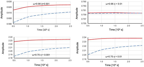
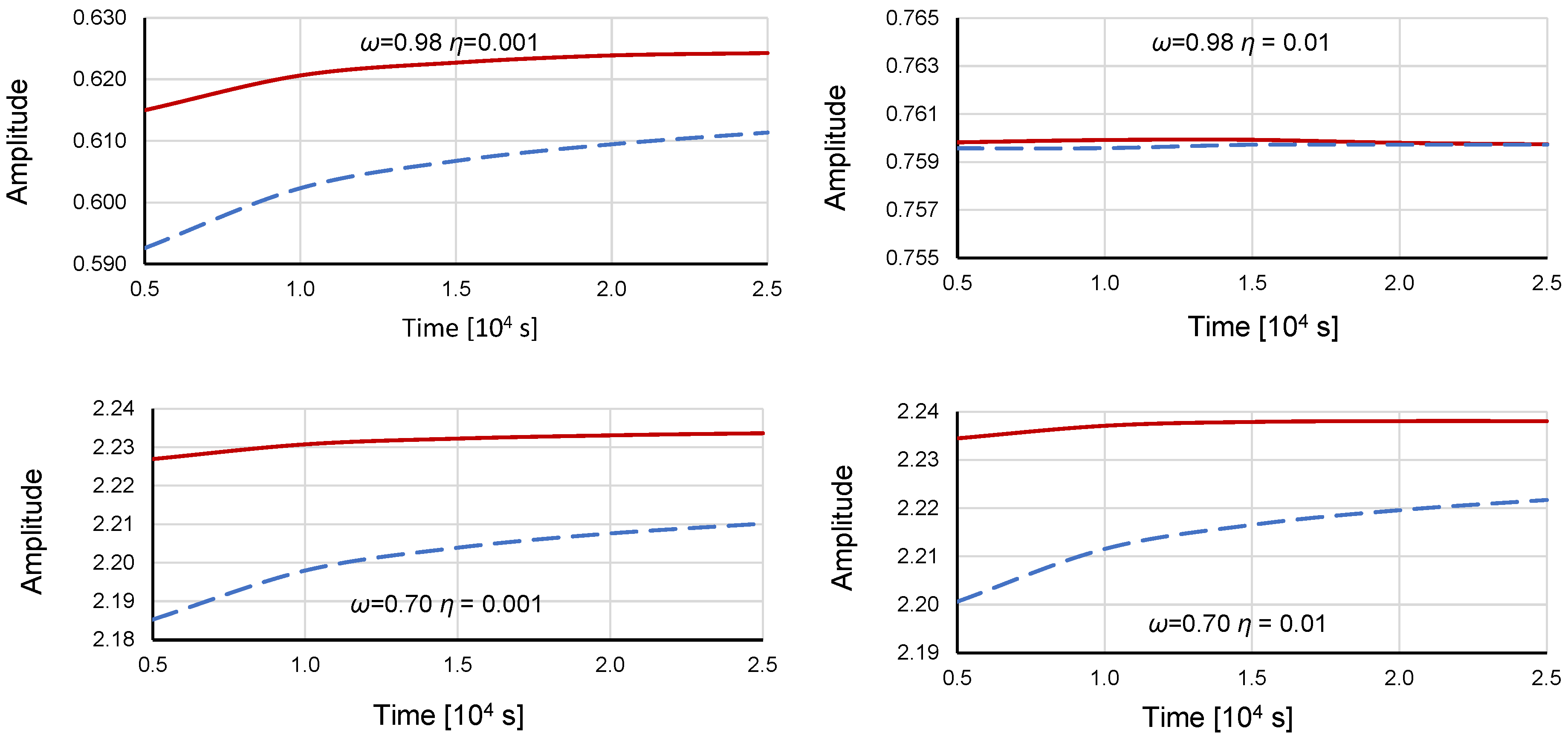
The dependence of the lower boundary of the unstable region on the rate of excitation increase is presented in Figure 4 for DE (4) with α = 1.000 and β = −0.045 for two frequencies: ω = 0.98 rad/s and ω = 0.70 rad/s. DE (4) is clearly sensitive to the rate of change in the excitation value for small damping values and for frequencies further from the system natural frequency ωn = 1.00 (Figure 4). However, above a certain damping value, namely, η > 0.005 at ω = 0.98 and η > 0.04 at ω = 0.70, the rate of change in the excitation value becomes irrelevant. Increasing the excitation value according to a sine function yielded better results (a higher position of the lower boundary of the unstable region). Considering the results of the tests carried out, all numerical simulations were performed with the excitation value increasing according to a sine function within the first 20,000 seconds of the simulation.
Figure 4.
Dependence of the lower boundary of the unstable region on the damping value, time period and form of excitation increase (solid line: sine increase; dashed line: linear increase). Numerical simulations were performed using Equation (4) (α = 1.000, β = −0.045) for frequencies ω = 0.98 and ω = 0.70 rad/s. (https://data.mendeley.com/datasets/53v7m3xd44/1 data_2.xlsx, accessed on 29 September 2025).
4. Data Analysis
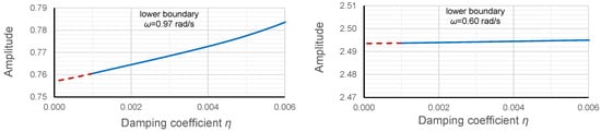
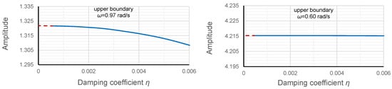
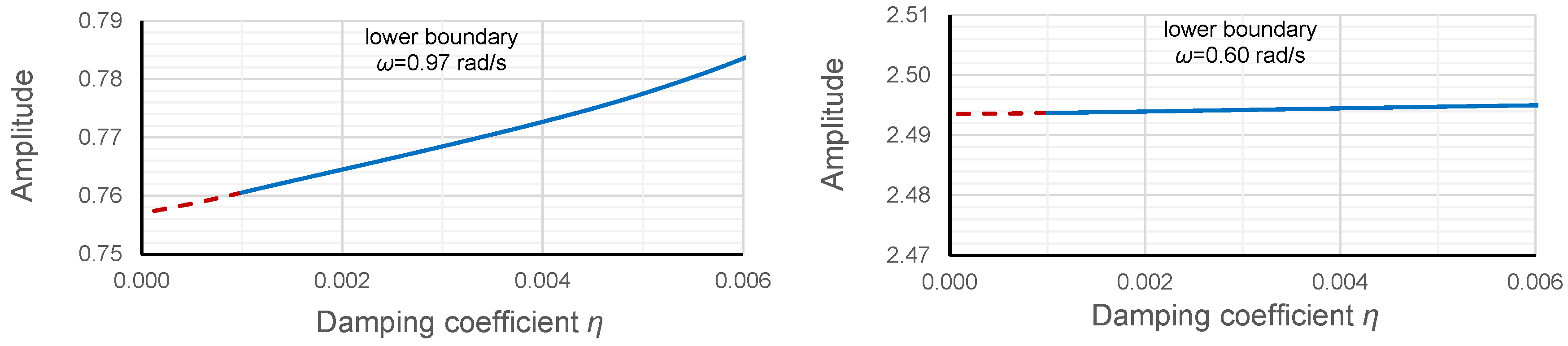
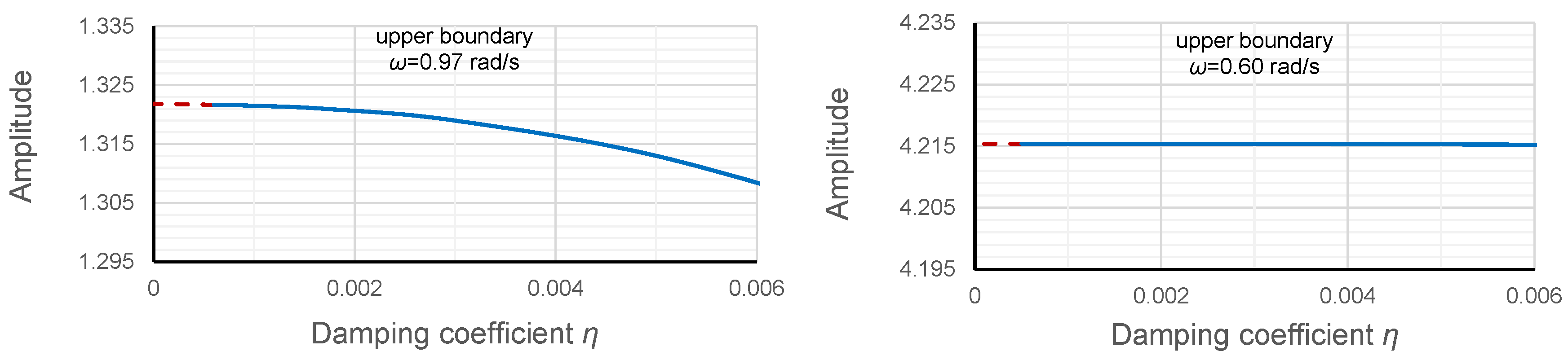
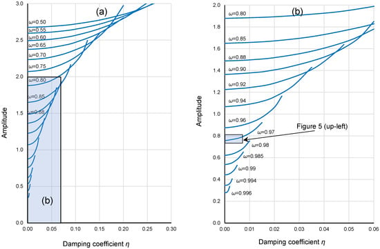
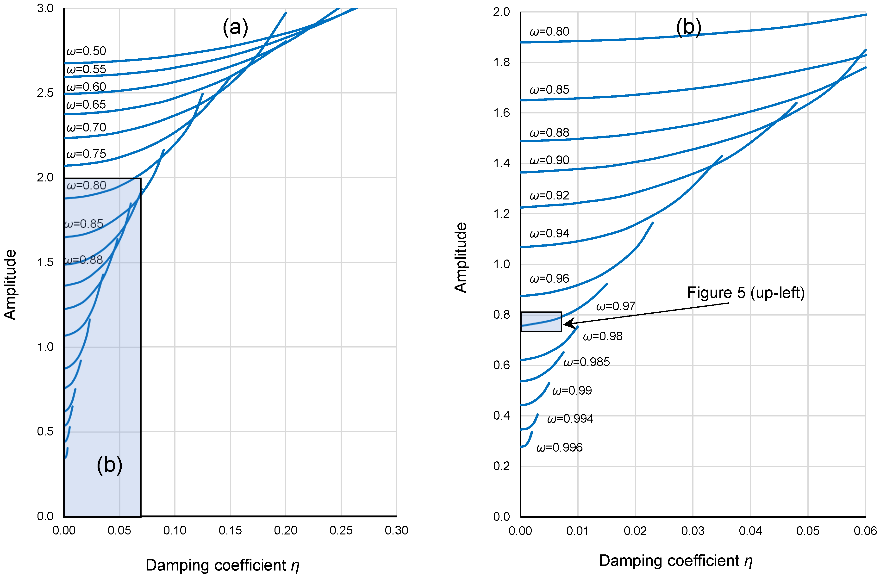
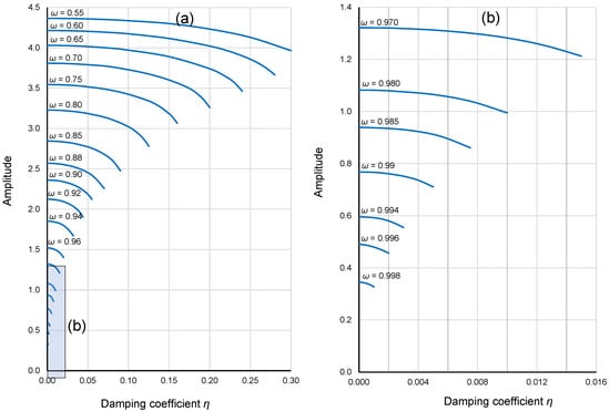
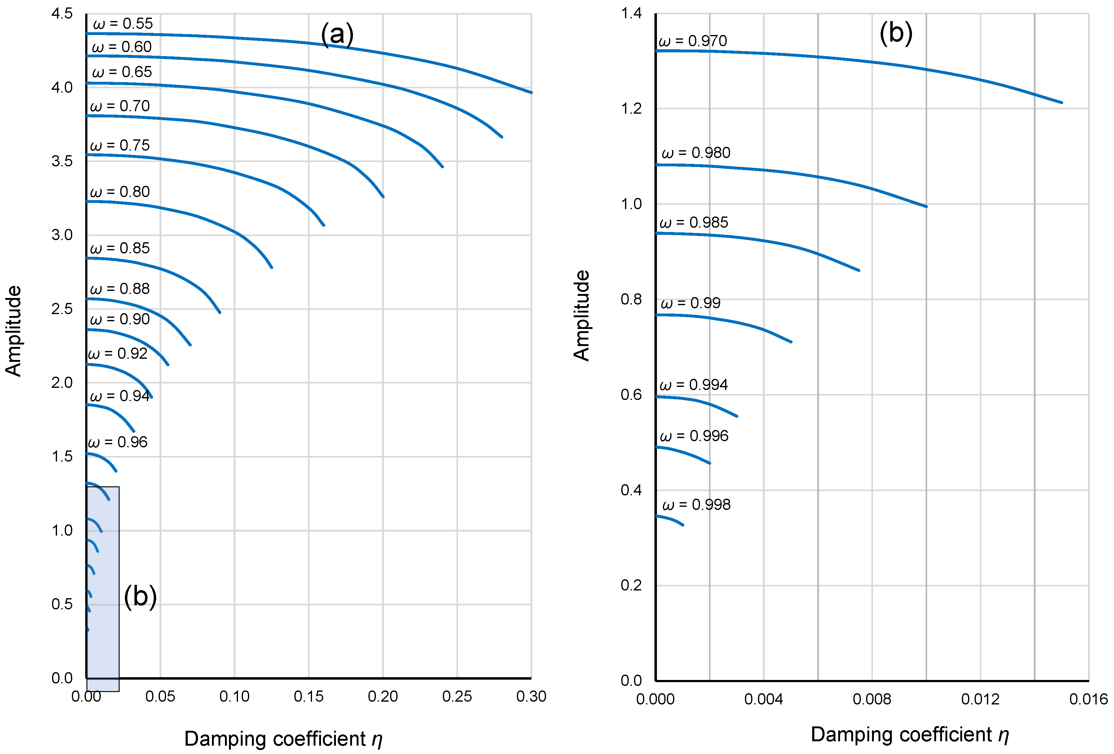
Directly determining the upper and lower limits of the unstable region for any dynamical system for damping equal to 0 using a numerical method is impossible. The issue is obtaining a stable solution (constant amplitude of oscillations). Therefore, a different approach was used in this research. For the given frequencies, the lower and upper limits of the unstable region were determined for a series of damping values, starting from high damping values and successively reducing them to the lowest values for which a stable solution could be obtained. Most often, the lowest value of η with stable oscillations was between 0.0003 and 0.001. Finally, the oscillation amplitude for η = 0 was graphically estimated, as shown in Figure 5. Based on a comparison of the left and right drawings (the scale is the same) in Figure 5, at lower frequencies (frequencies further from the natural frequency ωn), the sensitivity of the system to damping is much lower.
Figure 5.
Dependence of the lower and upper boundaries of the unstable region on the damping value for DE (1) with α = 1.000 and β = −0.045 for ω = 0.97 rad/s and 0.60 rad/s. The red dashed line is graphically estimated. (https://data.mendeley.com/datasets/53v7m3xd44/1 data_3.xlsx, accessed on 29 September 2025).
The results of procedure described above, for selected frequencies, are shown in Figure 6 (lower limit of the unstable region) and Figure 7 (upper limit of the unstable region).
Figure 6.
Dependence of the lower boundary of the unstable region on the damping value for DE (1) with α = 1.000, β = −0.045 for various frequencies; (a) all frequencies that have been tested; (b) frequencies > 0.75 rad/s. (https://data.mendeley.com/datasets/53v7m3xd44/1 data_3.xlsx, accessed on 29 September 2025).
Figure 7.
Dependence of the upper boundary of the unstable region on the damping value for DE (1) with α = 1.000, β = −0.045 for various frequencies; (a) all frequencies that have been tested; (b) frequencies > 0.75 rad/s. (https://data.mendeley.com/datasets/53v7m3xd44/1 data_3.xlsx, accessed on 29 September 2025).
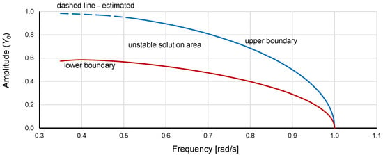
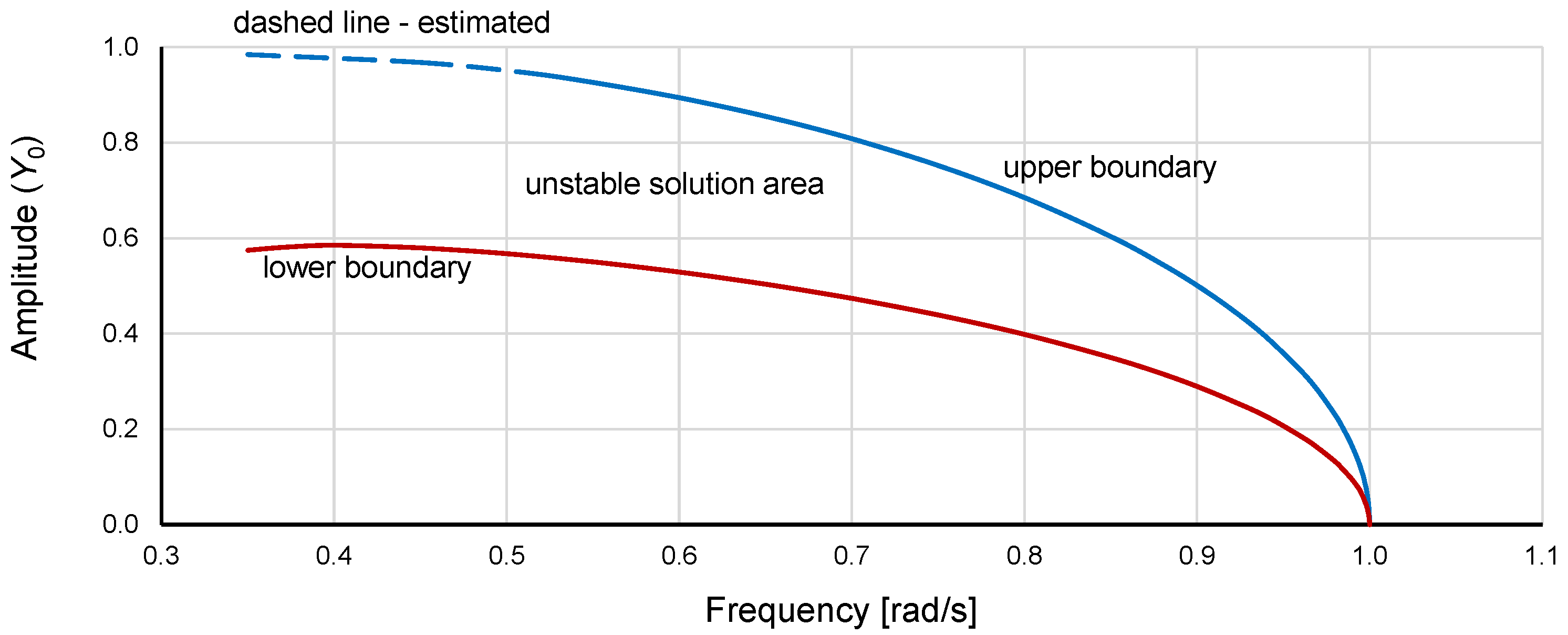
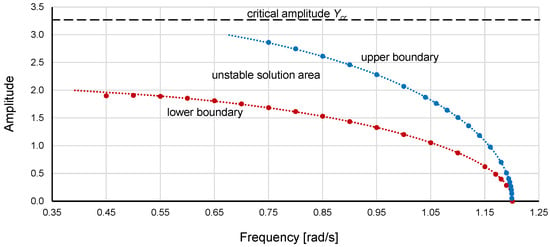
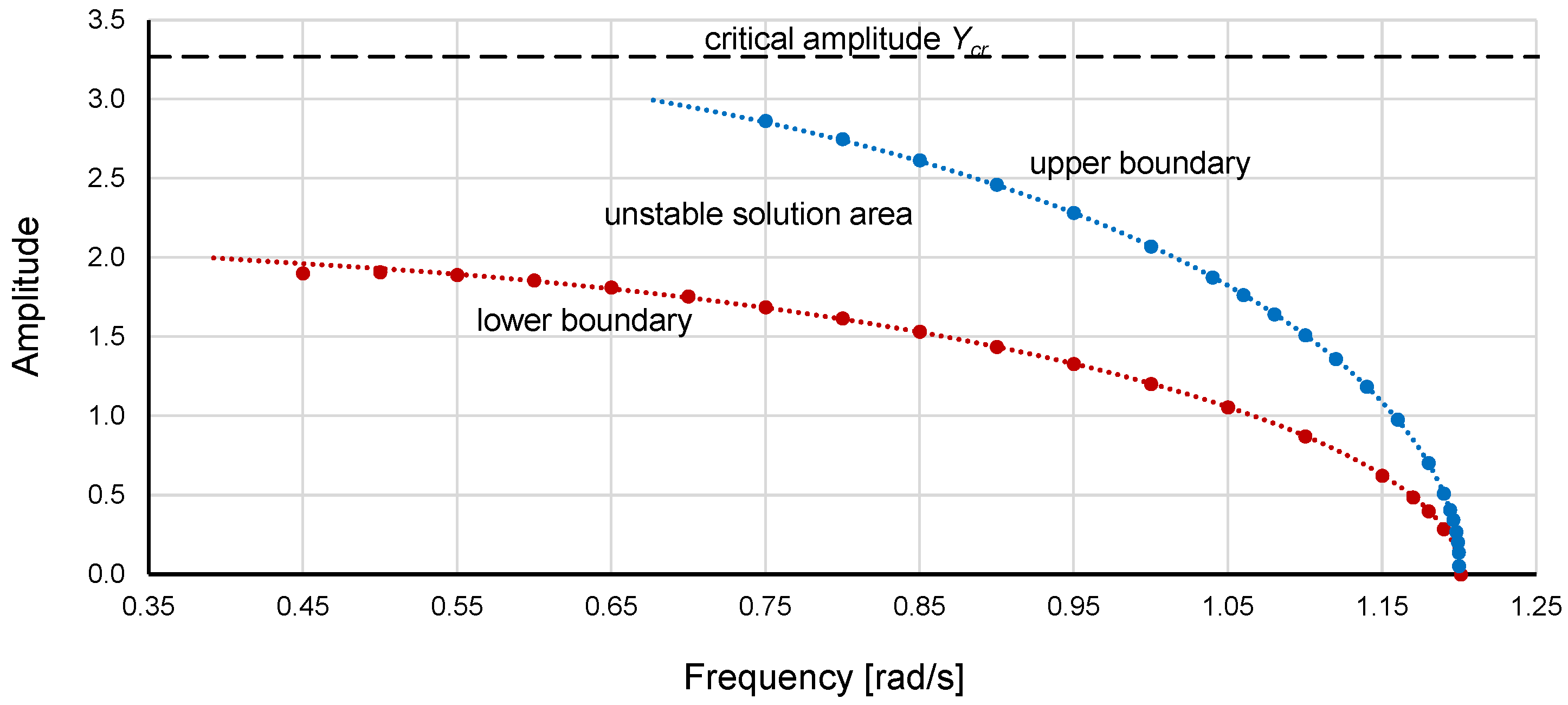
Based on the graphs shown in Figure 6 and Figure 7, the curves of the lower and upper boundaries of the unstable region of DE (1) were determined for α = 1.000, β = −0.045 and damping coefficient η = 0. These curves, scaled to a nondimensional form according to rule (6) [26,27], are presented in Figure 8.
Figure 8.
Upper and lower boundaries of the unstable region of DE (1) for α = 1.000, β = −0.045 and damping coefficient η = 0. The amplitude is scaled to a nondimensional form according to rule (6). (https://data.mendeley.com/datasets/53v7m3xd44/1 data_1.xlsx, accessed on 29 September 2025).
Notably, for the hardening system (α > 0 and β > 0), the critical amplitude does not exist, so scaling such systems using rule (6) is impossible.
Typically, an approximate solution to a nonlinear differential equation takes the form of an inverse function. This approach was also used in this research; the desired function was as follows: ω2 = 1 + c2·Y2 + c3·Y3 + … + cn·Yn. On the right side, the second power term determines the initial slope of the curve, whereas the terms with higher powers bend the curve at higher values of Y. Using the fitting procedure, formulas for the lower and upper boundaries of the unstable region were developed:
To consider the coefficient α, multiplying the right side of (7) and (8) by α is sufficient:
The use of Equations (7)–(10) is limited to the values of Y0 that correspond to ω ≥ 0.
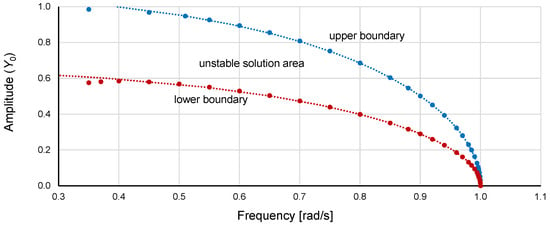
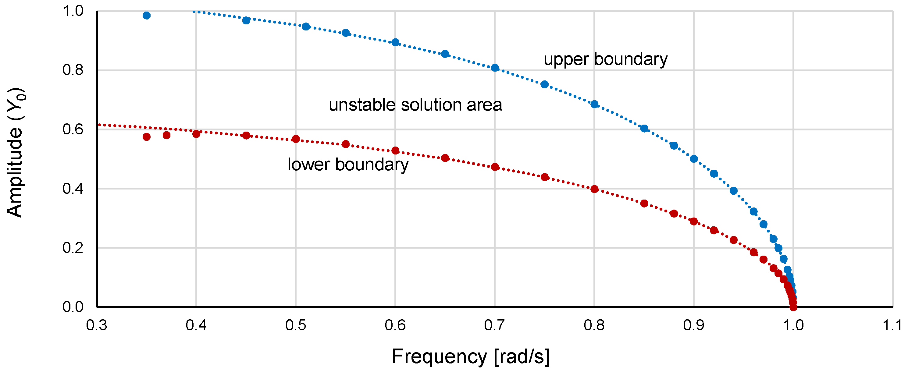
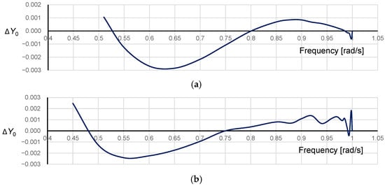
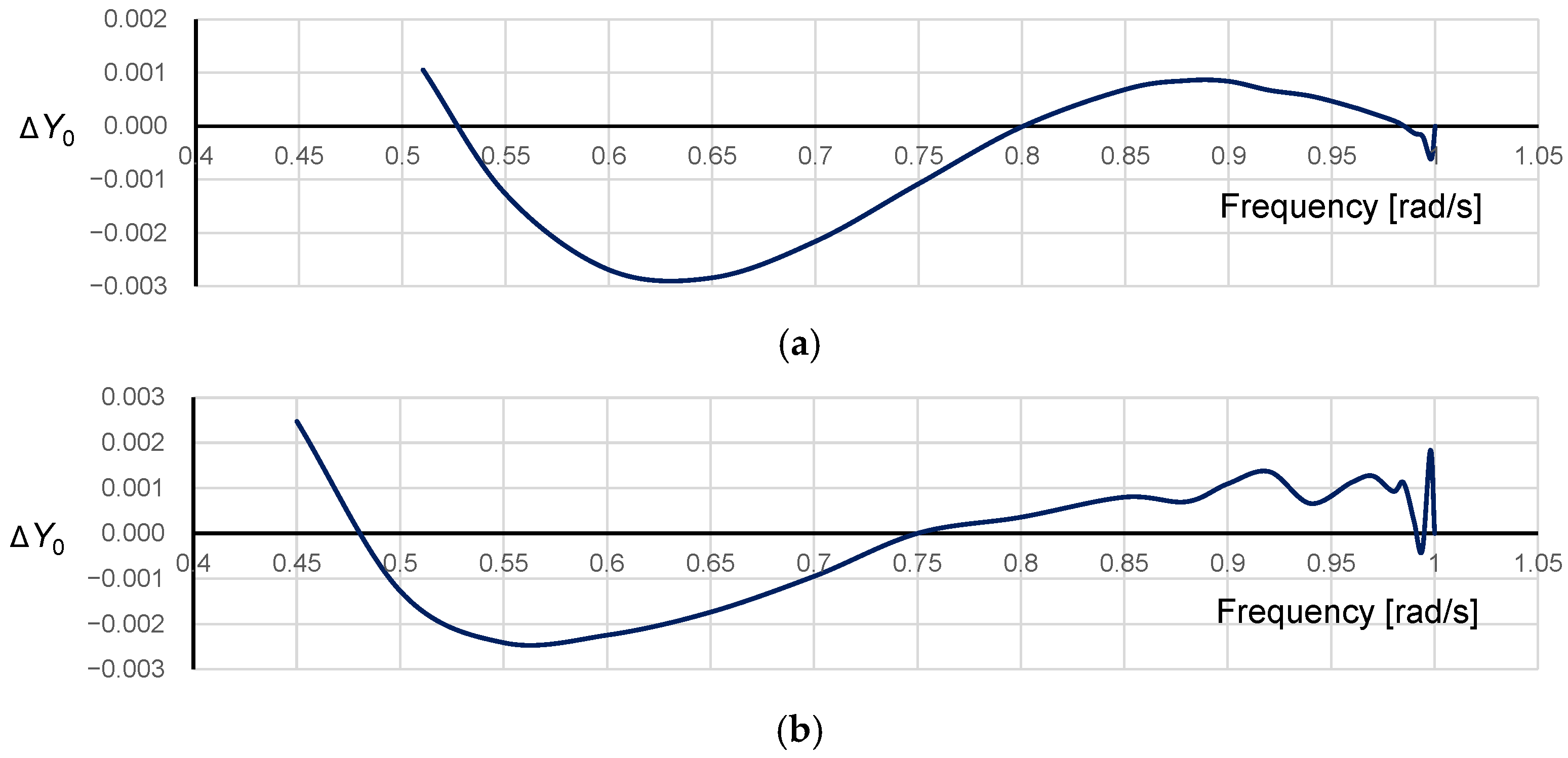
Graphs determined by Equations (7) and (8) are plotted with the data obtained using numerical simulations in Figure 9 to evaluate the consistency. As shown in the figure, good agreement occurs in the range from the natural frequency ωn (1.00 rad/s) down to 0.45 rad/s. Excluding frequencies below 0.45 rad/s, the differences between the developed formulas and numerical simulation results are very small, as shown in Figure 10.
Figure 9.
Consistency of Equations (9) and (10) with the data obtained using numerical simulations (markers) for DE (1) with α = 1.000, β = −0.045 and damping coefficient η = 0 (with the amplitudes scaled to a nondimensional form). (https://data.mendeley.com/datasets/53v7m3xd44/1 data_1.xlsx, accessed on 29 September 2025).
Figure 10.
Differences between the upper (a) and lower (b) boundaries of the unstable region, calculated using Equations (9) and (10), and the results of numerical simulations for Duffing equation (1) with α = 1.000, β = −0.045 and damping coefficient η = 0 (nondimensional form). (https://data.mendeley.com/datasets/53v7m3xd44/1 data_3.xlsx, accessed on 29 September 2025).
Equations (9) and (10), which were determined for the nondimensional value of the amplitude Y0, can be used for the Duffing equation with any values of α and β with only one restriction—the damping coefficient η = 0. Returning to the curves at the original scale, the final formulas for the lower and upper boundaries of the unstable region are:
and considering the sign of β (softening systems),
The use of Equations (11)–(14) is limited to values of Y that correspond to ω = 0.
The consistency of Equations (13) and (14) with the data obtained using numerical simulations was tested for the Duffing equation with a damping coefficient η = 0 for several combinations of α and β, with good results, such as those shown in Figure 11.
Figure 11.
Consistency of Equations (13) and (14) with the data obtained using numerical simulations (markers) for the Duffing equation with α = 1.44225, β = −0.135 and damping coefficient η = 0 (original scale). (https://data.mendeley.com/datasets/53v7m3xd44/1 data_1.xlsx, accessed on 29 September 2025).
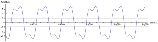
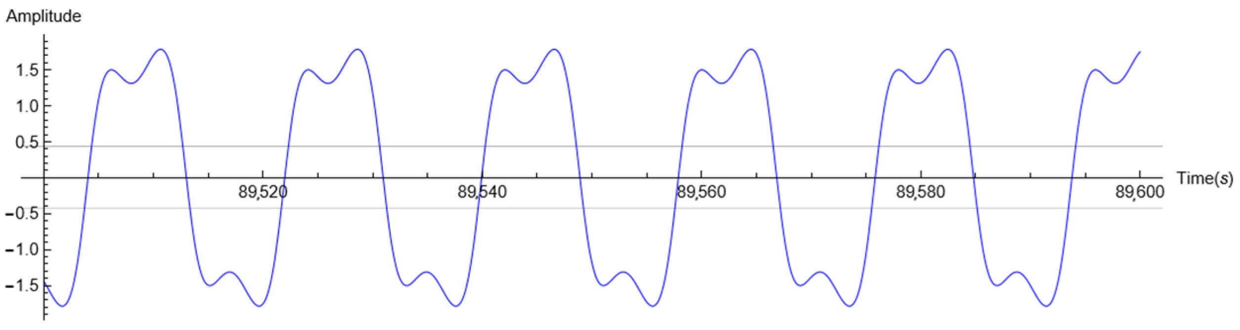
Differences between the developed formulas and the results of the numerical simulations for frequencies below 0.45 rad/s, as shown in Figure 9 and Figure 11, were identified for all the tested cases. Since the natural frequency ωn for each case was different, these differences were not related to the distance from ωn of a given case. The reason is that for low frequencies, the simulation result was no longer a pure sine wave (Figure 12).
Figure 12.
Oscillation time history for DE (1) with η = 0.06, α = 1.44225, β = −0.135, ω = 0.35 and excitation coefficient ξ = 1.88.
In Figure 8 and Figure 9, only the amplitude (displacement) value is in nondimensional form. To scale the frequency to a nondimensional form, rule (15) is commonly used.
For damping equal to 0, by using Y0 and ω0 according to rules (6) and (15), respectively, identical graphs of the upper and lower boundaries of the unstable region were obtained in all cases (Table 1), exactly as in Figure 9. This leads to the conclusion that for damping equal to 0, systems described by DE (1) with different parameters have the same instability regions in dimensionless space.
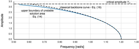
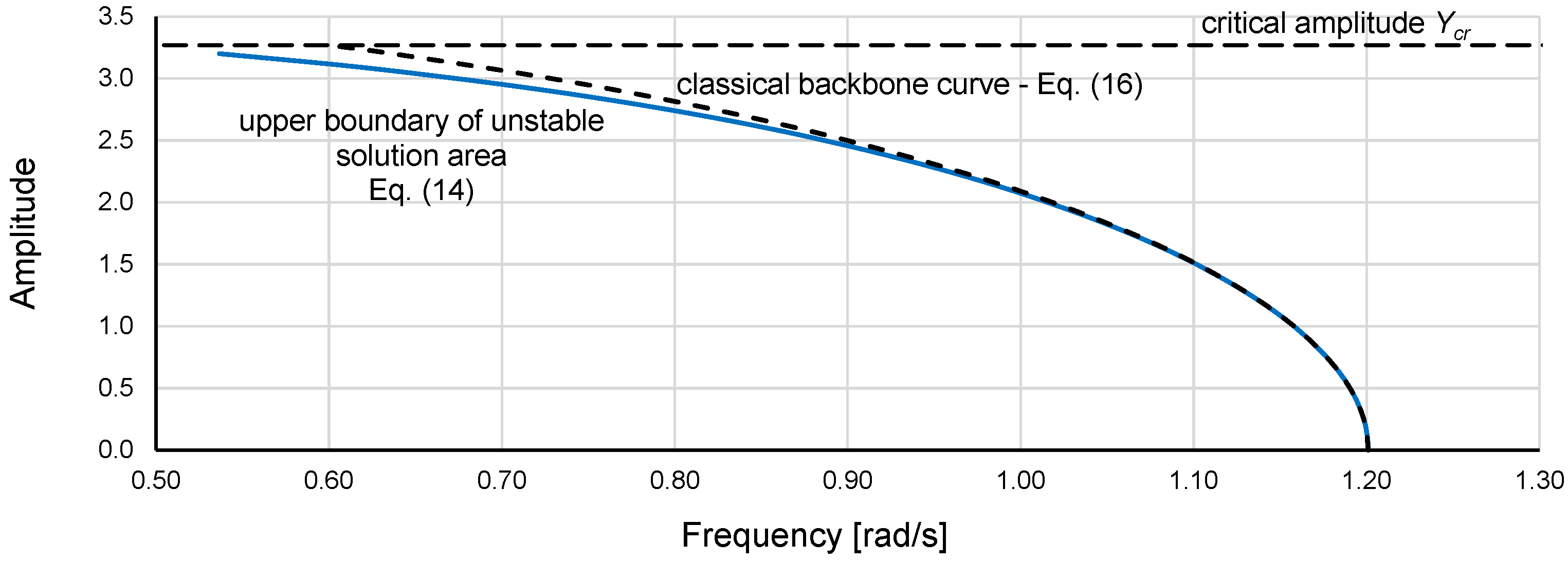
In the analysis of nonlinear dynamical systems, a backbone curve (16) is often used [28]. It represents the natural frequency of a system as a function of the amplitude of the system response when neither damping nor forcing is present and provides a valuable description of the system dynamics that can be very useful [29,30]. However, more importantly, the backbone curve is defined as the jump-down curve [28]. Figure 13 shows the consistency between the upper boundary of the unstable region for η = 0 obtained using numerical simulations and approximated by Equation (14) and the classical backbone curve calculated using Equation (16), which is commonly used and was derived via an analytical method. Since the backbone curve is a jump-down curve, it should have the same course as the curve of the upper boundary of the unstable region (14). However, high consistency between the curves can be observed only at small and medium amplitudes. This consistency is related to the fact that the first 2 terms of Equation (14) are equal to the complete Equation (16). The higher-power terms in Equation (14) have negligible effects at small and medium amplitudes and bend the curve mostly at higher amplitudes. The inconsistencies between the upper boundary of the unstable region and the backbone curve calculated using Equation (16) were previously observed [26].
Figure 13.
Classical backbone curve (16) and upper boundary of the unstable region for DE (1) with α = 1.44225, β = −0.135 and damping coefficient η = 0, calculated using Equation (14). (https://data.mendeley.com/datasets/53v7m3xd44/1 data_1.xlsx, accessed on 29 September 2025).
As mentioned above, lack of consistency of the classical backbone curve (16) with the upper boundary of the unstable region obtained using numerical simulations occurred in all cases that have been tested. It could therefore be concluded that the backbone curve is not equal to the upper boundary of the unstable region.
The boundaries of the unstable region determined by Equations (13) and (14) can be used to check whether formulas derived via analytical methods indicate the exact jump-up and jump-down loci. It may seem obvious that such verification should be performed for very small damping values, but Figure 7 and Figure 8 show that for frequencies not too close to the natural frequency ωn, the applied value of the η coefficient can even be 0.01.
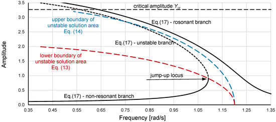
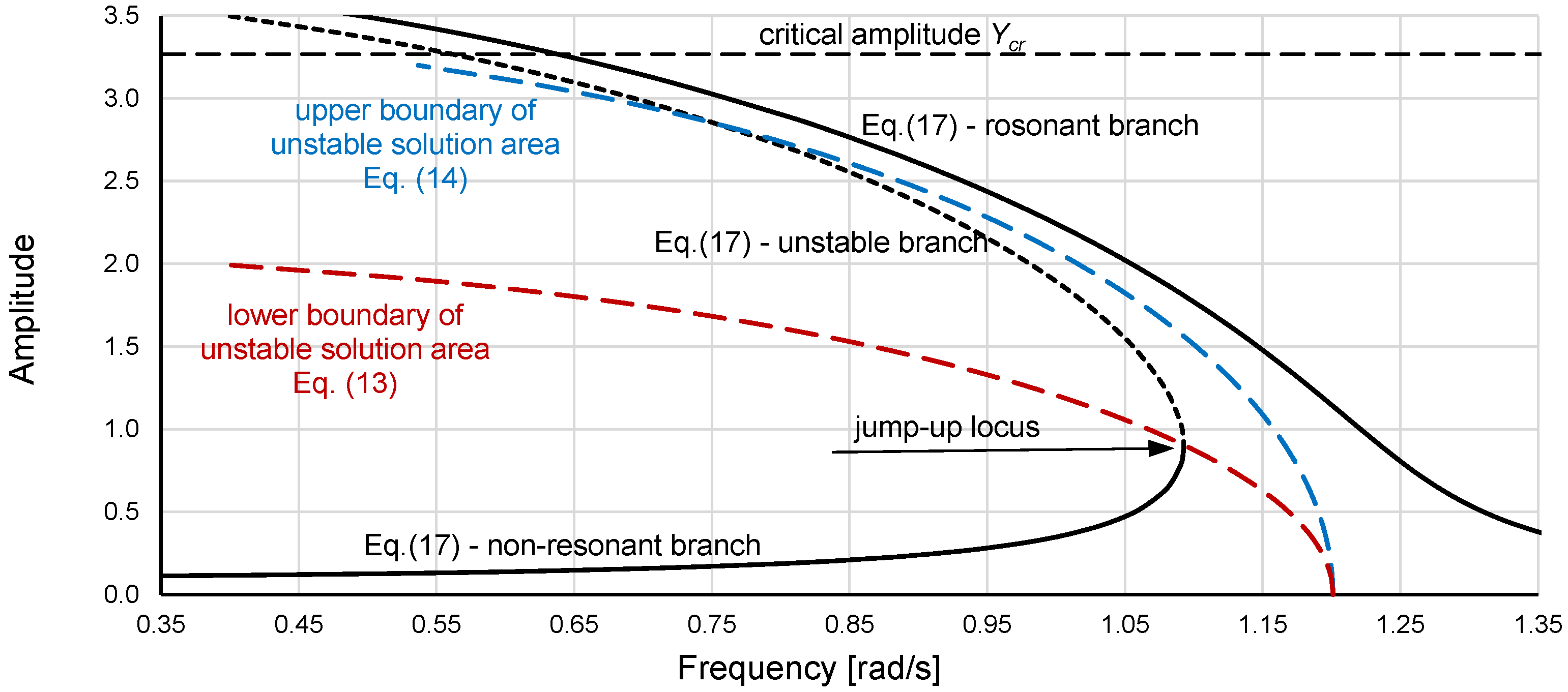
As an example, Figure 14 shows the unstable region for DE (1) with α = 1.44225, β = −0.135, and η = 0 calculated using Equations (13) and (14) and the frequency response curve determined for the same α and β but η = 0.0001 by using the formula derived via the homotopy analysis method [31]:
Figure 14.
Boundaries of the unstable region of DE (1) with α = 1.44225, β = −0.135, and η = 0 calculated using Equations (13) and (14), and the frequency response curve determined using Equation (17) for the same α and β but η = 0.0001 and excitation coefficient ξ = 0.15. (https://data.mendeley.com/datasets/53v7m3xd44/1 data_1.xlsx, accessed on 29 September 2025).
Equation (17) provides a graph with 3 branches (Figure 14). The two basic branches are the resonant branch and nonresonant branch (black solid lines), and the third branch is the branch in the unstable region—the unstable branch (black dashed line). The jump-up locus for Equation (17) is at the junction of the nonresonant branch and unstable branch. Figure 14 clearly shows that it is positioned at the lower boundary of the unstable region, so it is correctly determined. Unfortunately, in the higher-amplitude region (Figure 14), the paths of the resonant branch and unstable branch seem to be incorrect. Only part of the unstable branch is located in the unstable region, whereas its upper part is in the stable region. More importantly, Equation (17) does not reveal a jump-down—the jump-down locus should be indicated by the junction of the resonant and unstable branches.
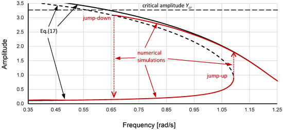
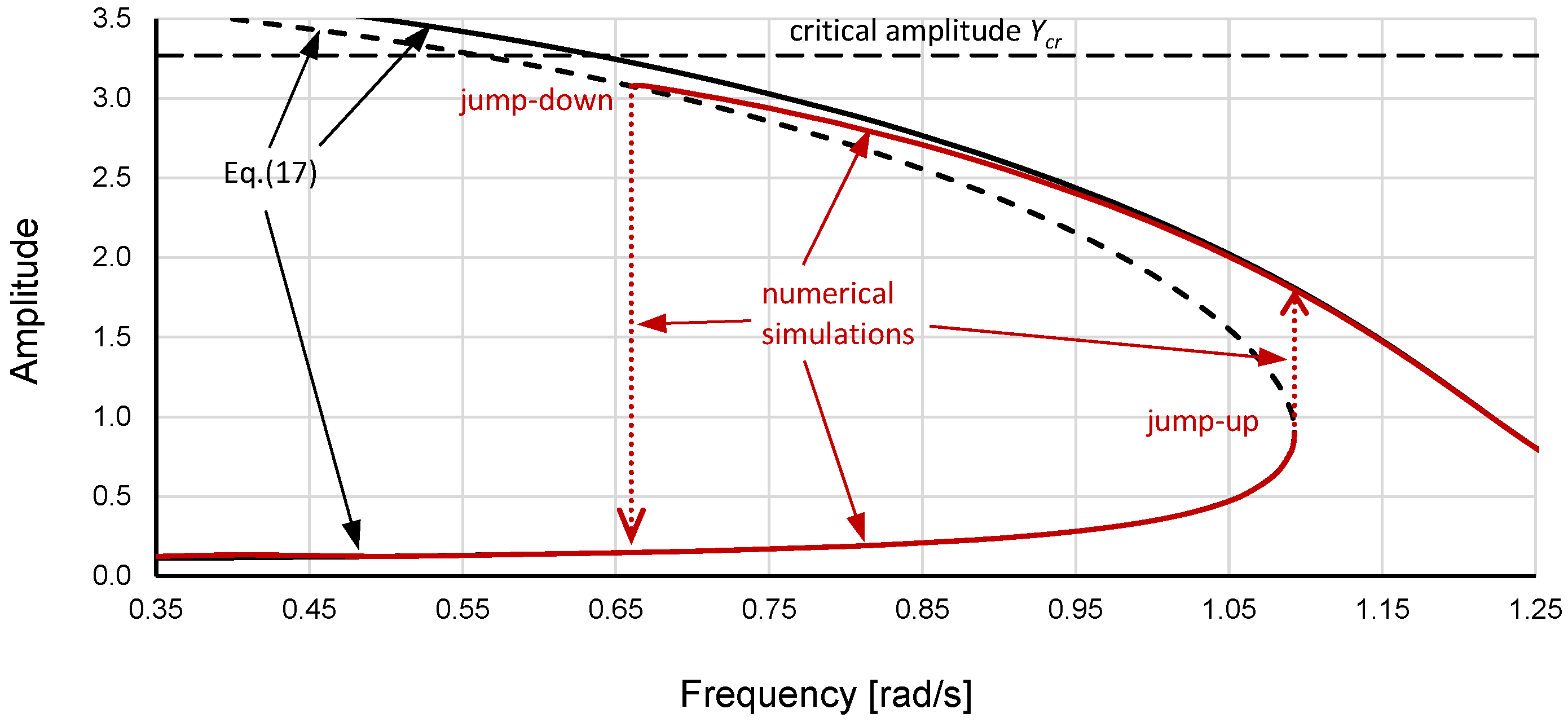
A comparison of the graphs calculated using Equation (17) with the results of numerical simulations for DE (1) (Figure 15) reveals that Equation (17) does not actually determine the correct course of the resonant branch in the higher-amplitude region. Additionally, Equation (17) was tested with various damping and excitation values and does not reveal a jump-down regardless of the η or ξ value.
Figure 15.
Frequency response curves for DE (1) with α = 1.44225, β = −0.135, η = 0.0001 and excitation coefficient ξ = 0.15 determined using Equation (17) (black solid and dashed lines) and numerical simulations (red solid and dotted lines–the dotted lines indicate amplitude jumps). (https://data.mendeley.com/datasets/53v7m3xd44/1 data_1.xlsx, accessed on 29 September 2025).
5. Conclusions
In this study, the standard Duffing equation with softening stiffness was analyzed. Using numerical simulations, the upper and lower boundaries of the unstable region for damping equal to 0 were identified, and Equations (13) and (14) that describe them were developed. The results of the analysis show that the developed equations are effective for all combinations of the stiffness coefficients that have been tested. Notably, the nondimensional forms of the unstable region for damping equal to 0 (scaled according to (6) and (15)) for all cases are identical. Equations (13) and (14) can also be helpful in developing analytic formulas for the upper and lower limits of the unstable region considering non-zero damping.
The curve of the upper boundary of the unstable region can be calculated using Equation (14), which was developed during this research. Since it is a jump-down curve, its course should be the same as that of the classical backbone curve, which is commonly calculated using Equation (16) derived via analytical methods. The calculation results of (14) and (16) were compared, and high consistency between them occurred only at small and medium amplitudes because the first two terms of Equation (14) are identical to the complete Equation (16), whereas the last two terms of Equation (14) consider additional changes that occur at higher amplitudes and have negligible effects at small and medium amplitudes. Notably, the results of numerical simulations are more credible than the results of calculations with formulas derived via analytical methods. It could therefore be concluded that the backbone curve is not equal to the upper boundary of the unstable solution region.
The additional purpose of this paper is to provide the results of numerical simulations (not just graphs). Furthermore, the included data (Excel files) can be used to derive new and verify existing analytical formulas for the standard Duffing equation. Each figure included in this study to present the results of numerical simulations carried out during the research is accompanied by the name of a file that contains the data used to prepare it. Notably, the attached files contain more data than presented in the paper (and not only for damping equal to 0), and they are described accordingly.
Funding
This study was financed by the Gdynia Maritime University, the research project WN/2024/PZ/03.
Institutional Review Board Statement
Not applicable.
Informed Consent Statement
Not applicable.
Data Availability Statement
Data obtained during the research and used to prepare the paper have been deposited in the Mendeley Data repository and is publicly available at https://data.mendeley.com/datasets/53v7m3xd44/1 (accessed on 29 September 2025).
Conflicts of Interest
The author declares no competing interests.
References
- Duffing, G. Forced Oscillations with Variable Natural Frequency and Their Technical Relevance; Heft 41/42; Vieweg: Braunschweig, Germany, 1918. (In German) [Google Scholar]
- Li, L.; Chen, J. Characterization of cracking-healing cycle of asphalt mixture based on air-coupled second harmonic measurement using Duffing-van der pol oscillator. Mech. Syst. Signal Process. 2024, 216, 111516. [Google Scholar] [CrossRef] [Scilit]
- Xiang, J.; Guo, J.; Li, X. A two-stage Duffing equation-based oscillator and stochastic resonance for mechanical fault diagnosis. Chaos Solitons Fractals 2024, 182, 114755. [Google Scholar] [CrossRef] [Scilit]
- Manh, N.; Linh, N.; Nguyen, A.; Anh, N. Higher-order averaging procedure for performance analysis of a mono-stable Duffing piezoelectric energy harvesting system under white noise excitation. Mech. Res. Commun. 2023, 131, 104157. [Google Scholar] [CrossRef] [Scilit]
- Zhang, W.; Wang, T.; Han, X.; Zhang, S.; Wang, H. Mechanical squeezing induced by Duffing nonlinearity and two driving tones in an optomechanical system. Phys. Lett. A 2022, 424, 127824. [Google Scholar] [CrossRef] [Scilit]
- Huang, W.; Yu, Y.; Tong, C.; Xu, M.; Zhang, R. Using a Duffing control approach to control the single risk factor in complex social-technical systems. Inf. Sci. 2022, 596, 264–279. [Google Scholar] [CrossRef] [Scilit]
- Song, J. Effects of modulation phase on relaxation oscillations in the Duffing system. Chaos Solitons Fractals 2024, 178, 114350. [Google Scholar] [CrossRef] [Scilit]
- Coccolo, M.; Seoane, J.M.; Sanjuan, M.A. Fractional damping induces resonant behavior in the Duffing. Commun. Nonlinear Sci. Numer. Simul. 2024, 133, 107965. [Google Scholar] [CrossRef] [Scilit]
- Lenci, S. Exact solutions for coupled Duffing oscillators. Mech. Syst. Signal Process. 2022, 165, 108299. [Google Scholar] [CrossRef] [Scilit]
- Kovacic, I. Externally excited undamped and damped linear and nonlinear oscillators: Exact solutions and tuning to a desired exact form of the response. Int. J. Nonlinear Mech. 2018, 102, 72–81. [Google Scholar] [CrossRef] [Scilit]
- Zakeri, G.; Yomba, E. Exact solutions of a generalized autonomous Duffing-type equation. Appl. Math. Model. 2015, 39, 4607–4616. [Google Scholar] [CrossRef] [Scilit]
- Azimi, M. Stability and bifurcation of Mathieu–Duffing equation. Int. J. Non-Linear Mech. 2022, 144, 104049. [Google Scholar] [CrossRef] [Scilit]
- Liu, L.; Thomas, J.; Dowell, E.; Attar, P.; Hall, K. A comparison of classical and high dimensional harmonic balance approaches for a Duffing oscillator. J. Comput. Phys. 2006, 215, 298–320. [Google Scholar] [CrossRef] [Scilit]
- Grolet, A.; Thouverez, F. On a new harmonic selection technique for harmonic balance method. Mech. Syst. Signal Process. 2012, 30, 43–60. [Google Scholar] [CrossRef] [Scilit]
- Mickens, R.E. A generalized iteration procedure for calculating approximations to periodic solutions of truly nonlinear oscillators. J. Sound Vib. 2005, 287, 1045–1051. [Google Scholar] [CrossRef] [Scilit]
- Chen, S.H.; Cheung, Y.K.; Lau, S.L. On perturbation procedure for limit cycle analysis. Int. J. Non-Linear Mech. 1991, 26, 125–133. [Google Scholar] [CrossRef] [Scilit]
- Cveticanin, L. Homotopy-perturbation method for pure nonlinear differential equation. Chaos Solitons Fractals 2006, 30, 1221–1230. [Google Scholar] [CrossRef] [Scilit]
- Leung, A.Y.T.; Guo, Z. Homotopy perturbation for conservative Helmholtz–Duffing oscillators. J. Sound Vib. 2009, 325, 287–296. [Google Scholar] [CrossRef] [Scilit]
- Van Dooren, R.; Janssen, H. A continuation algorithm for discovering new chaotic motions in forced Duffing systems. J. Comput. Appl. Math. 1996, 66, 527–541. [Google Scholar] [CrossRef] [Scilit]
- Starosta, R.; Sypniewska-Kaminska, G.; Awrejcewicz, J. Quantifying non-linear dynamics of mass-springs in series oscillators via asymptotic approach. Mech. Syst. Signal Process. 2017, 89, 149–158. [Google Scholar] [CrossRef] [Scilit]
- Wawrzyński, W. Bistability and accompanying phenomena in the 1-DOF mathematical model of rolling. Ocean Eng. 2018, 147, 565–579. [Google Scholar] [CrossRef] [Scilit]
- Kamiński, M.; Corigliano, A. Numerical solution of the Duffing equation with random coefficients. Meccanica 2015, 50, 1841–1853. [Google Scholar] [CrossRef] [Scilit]
- Agarwal, V.; Zheng, X.; Balachandran, B. Influence of noise on frequency responses of softening Duffing oscillators. Phys. Lett. A 2018, 382, 3355–3364. [Google Scholar] [CrossRef] [Scilit]
- Ramlan, R.; Brennan, M.J.; Kovacic, I.; Mace, B.R.; Burrow, S.G. Exploiting knowledge of jump-up and jump-down frequencies to determine the parameters of a Duffing oscillator. Commun. Nonlinear Sci. Numer. Simul. 2016, 37, 282–291. [Google Scholar] [CrossRef] [Scilit]
- Contento, G.; Francescutto, A.; Piciullo, M. On the Effectiveness of Constant Coefficients Roll Motion Equation. Ocean Eng. 1996, 23, 597–618. [Google Scholar] [CrossRef] [Scilit]
- Wawrzynski, W. Duffing-type oscillator under harmonic excitation with a variable value of excitation amplitude and time dependent external disturbances. Sci. Rep. 2021, 11, 288. [Google Scholar] [CrossRef] [Scilit]
- Wawrzyński, W. The origin point of the unstable solution area of a forced softening Duffing oscillator. Sci. Rep. 2022, 12, 4518. [Google Scholar] [CrossRef] [Scilit]
- Brennan, M.J.; Kovacic, I.; Carrella, A.; Waters, T.P. On the jump-up and jump-down frequencies of the Duffing oscillator. J. Sound Vib. 2008, 318, 1250–1261. [Google Scholar] [CrossRef] [Scilit]
- Chen, Q.M.; Fischer, M.; Nojiri, Y.; Renger, M.; Xie, E.; Partanen, M.; Pogorzalek, S.; Fedorov, K.G.; Marx, A.; Deppe, F.; et al. Quantum behavior of the Duffing oscillator at the dissipative phase transition. Nat. Commun. 2023, 14, 2896. [Google Scholar] [CrossRef] [Scilit]
- Londoño, J.M.; Neild, S.A.; Cooper, J.C. Identification of backbone curves of nonlinear systems from resonance decay responses. J. Sound Vib. 2015, 348, 224–238. [Google Scholar] [CrossRef] [Scilit]
- Jordan, D.W.; Smith, P. Nonlinear Ordinary Differential Equations: An Introduction for Scientists and Engineers; Oxford University Press: Oxford, UK, 2007. [Google Scholar]

Disclaimer/Publisher’s Note: The statements, opinions and data contained in all publications are solely those of the individual author(s) and contributor(s) and not of MDPI and/or the editor(s). MDPI and/or the editor(s) disclaim responsibility for any injury to people or property resulting from any ideas, methods, instructions or products referred to in the content. |
© 2026 by the author. Licensee MDPI, Basel, Switzerland. This article is an open access article distributed under the terms and conditions of the Creative Commons Attribution (CC BY) license.